





1. Introduction
Following the observation of self-propulsion of catalytic particles (Paxton et al. Reference Paxton, Kistler, Olmeda, Sen, Angelo, Cao, Mallouk, Lammert and Crespi2004), there has been ongoing interest in the possibility of self-sustained particle motion enabled by interfacial chemical reactions. The first theoretical description of such motion was provided by Golestanian, Liverpool & Ajdari (Reference Golestanian, Liverpool and Ajdari2007); it modelled the interfacial reactions by a specified distribution of solute flux at the particle boundary, while the interaction of the solute molecules with that boundary was described macroscopically using diffusio-osmotic slip (Anderson Reference Anderson1989). In their idealised model, solute is transported diffusively, unaffected by the flow. With the Stokes equations being adequate, the analysis amounts to the solution of two linear problems, one governing the solute transport and one governing the flow. In that setting, self-sustained particle motion necessitates either an asymmetric distribution of the interfacial reaction or an asymmetric geometry.
Several authors have extended the above idealised model by incorporating solute advection (Michelin & Lauga Reference Michelin and Lauga2014; Yariv & Michelin Reference Yariv and Michelin2015; Boniface et al. Reference Boniface, Cottin-Bizonne, Kervil, Ybert and Detcheverry2019). This extension renders the problem inherently nonlinear. The role of nonlinearity may be quantified by the characteristic ratio, say  $\alpha$, of advective and diffusive fluxes. Since the velocity scale associated with advection is not imposed externally,
 $\alpha$ constitutes an intrinsic Péclet number. One may perhaps expect that accounting for advection would merely result in more complicated analysis, with the underlying mechanism of self-propulsion remaining unaffected. It turns out, however, that advection gives rise to phenomena that are completely absent when solute transport is purely diffusive. One such example is two-dimensional propulsion (Sondak et al. Reference Sondak, Hawley, Heng, Vinsonhaler, Lauga and Thiffeault2016; Yariv Reference Yariv2017; Hu et al. Reference Hu, Lin, Rafai and Misbah2019; Yariv & Crowdy Reference Yariv and Crowdy2020), where the neglect of advection leads to an ill-posed problem. Another example, which is at the focus of the present paper, is the possibility of autophoresis of isotropic particles.
Consider in particular a spherical particle with a uniform chemical activity. The underlying spherical symmetry may appear to suggest that such a particle does not acquire any velocity as a result of the chemical activity. This is indeed true for diffusive transport, as is evident from the model of Golestanian et al. (Reference Golestanian, Liverpool and Ajdari2007). Michelin, Lauga & Bartolo (Reference Michelin, Lauga and Bartolo2013) have shown, however, that when solute advection is introduced, the nonlinear problem may admit non-trivial solutions past the critical value  $\alpha =4$, beyond which the stationary solution is unstable. The non-trivial solutions were shown to describe steady spontaneous motion of the particle in a random direction. In fact, similar such motion was later observed experimentally in an analogous physical system where the active solid particle is replaced by an active droplet, in which case the spontaneously formed non-uniform concentration field drives a flow via interfacial Marangoni stresses, rather than slip (Izri et al. Reference Izri, Van Der Linden, Michelin and Dauchot2014).
The theoretical models of Golestanian et al. (Reference Golestanian, Liverpool and Ajdari2007) and Michelin et al. (Reference Michelin, Lauga and Bartolo2013) assume a force-free active particle which is suspended in a quiescent fluid. In the specific case of a spherical particle with a uniform chemical activity, what is the effect of an externally imposed flow? It is clear that, in the absence of solute advection, the flow does not affect the solute-concentration profile. Conversely, the spherically symmetric solute distribution does not affect the flow. The response of the particle to the imposed fluid motion is therefore unaffected by the chemical reaction at its boundary. When advection is accounted for, however, the solute-transport and flow problems are nonlinearly coupled, and the response of the particle is affected by the reaction. Unlike the ‘unforced’ problem considered by Michelin et al. (Reference Michelin, Lauga and Bartolo2013), the ‘forced’ problem is characterised by two velocity scales, namely the ‘chemical’ scale associated with diffusio-osmosis and the ‘mechanical’ scale associated with the imposed flow.
The forced problem was addressed by Yariv & Kaynan (Reference Yariv and Kaynan2017) using a small- $\alpha$ linearisation, assuming that the external velocity scale is comparable to the chemical scale. Two modes of external forcing were considered: a uniform force field and an imposed shear flow. Given the underlying linearisation, the chemical activity has resulted in a small correction to the classical predictions of Stokes flow. In retrospect, a more interesting direction involves finite values of
 $\alpha$, where solute advection can result in significant modifications relative to these Stokes-flow predictions. An obvious additional benefit of the latter direction is that it also covers the range
 $\alpha >4$, where the stationary solution of the unforced problem is known to be unstable.
We here intend to pursue this direction for the case of an external force field. To allow for a tractable analysis, we plan to do so for the case where the external velocity scale is small compared with the chemical one. Away from the critical value  $\alpha =4$, this allows for a linearisation about the stationary solution that corresponds to the absence of a force field; in the neighbourhood of
 $\alpha =4$, the weak forcing naturally lends itself to a weakly nonlinear analysis which reveals the imperfect bifurcation at the critical Péclet number. Both the ‘global’ linearisation and the ‘local’ weakly nonlinear analysis require the use of matched asymptotic expansions in the spirit of classical forced-convection problems (Acrivos & Taylor Reference Acrivos and Taylor1962). Our approach resembles previous theoretical studies of weakly forced active droplets (Rednikov, Ryazantsev & Velárde Reference Rednikov, Ryazantsev and Velárde1994a,Reference Rednikov, Ryazantsev and Velárdeb,Reference Rednikov, Ryazantsev and Velárdec,Reference Rednikov, Ryazantsev and Velárded; Rednikov et al. Reference Rednikov, Kurdyumov, Ryazantsev and Velarde1995; Velarde, Rednikov & Ryazantsev Reference Velarde, Rednikov and Ryazantsev1996), whose mathematical description is partially similar to that of a spherical solid particle with a uniform chemical activity.
2. Physical problem
A homogeneous chemically active sphere of radius  $a$ is suspended in an unbounded liquid solution of concentration
 $c_\infty$. The interfacial chemical activity of the sphere is assumed uniform, and is represented by a solute flux
 ${j}$, which can be either positive or negative, depending on whether the sphere emits or absorbs solute. This prescribed flux results in the formation of an excess-solute cloud in the vicinity of the particle, where the difference between the local concentration and
 $c_\infty$ is of order
 \begin{equation} \mathcal{C} = \frac{a|{\,j}|}{D}, \end{equation}
with  $D$ being the solute diffusivity.
We employ a macroscale formulation (Michelin & Lauga Reference Michelin and Lauga2014) where interfacial gradients in the solute concentration are manifested in effective diffusio-osmotic slip. The associated slip coefficient is denoted by  $b$. We assume that
 $b$, too, is uniform. It can be positive or negative, corresponding to repulsive or attractive interactions between the solute molecules and the colloid boundary, respectively. The slip mechanism provides an intrinsic velocity scale
 \begin{equation} \mathcal{U}=\frac{|{\,j}b|}{D}. \end{equation}
Corresponding to that scale is the intrinsic Péclet number  $\alpha = a \mathcal {U} /D$, which, upon substitution of (2.2), is given by
 \begin{equation} \alpha = \frac{a |{\,j}b|}{D^{2}}. \end{equation}
This ratio quantifies the importance of solute advection relative to diffusion.
The problem isotropy suggests a solution where the excess-solute cloud surrounding the particle is spherically symmetric. Given that symmetry, no surface gradients of solute concentration are formed. With no interfacial slip, and in the absence of any other mechanism for flow generation, it follows that the above solution is stationary. Conversely, the absence of flow is compatible with the presumed spherically symmetric distribution of the solute concentration. That distribution is accordingly independent of  $\alpha$, and is determined by a purely diffusive mechanism, expressed by Laplace's equation.
The preceding picture changes when the problem is forced by an additional flow-generating mechanism. Qualitatively speaking, the forcing flow deforms the originally spherically symmetric solute cloud, associated with the unforced problem, into one that lacks such symmetry; in particular, it generates interfacial gradients of solute concentration. These, in turn, modify the flow through diffusio-osmotic slip. Denoting the velocity scale associated with the forcing by  $\mathcal {W}$, the dimensionless problem now depends (nonlinearly) upon both
 $\alpha$ and the ratio
 \begin{equation} \epsilon = \mathcal{W}/\mathcal{U} \end{equation}
of the mechanical and chemical scales (as well as the signs of  $j$ and
 $b$).
The present work addresses the asymptotic limit  $\epsilon \ll 1$ which constitutes a small perturbation to the unforced problem. Our approach is based upon perturbing the spherically symmetric solution of that problem. We allow for arbitrary
 $O(1)$ values of
 $\alpha$. This limit represents the interesting case where the chemical activity is significant, in the sense that it may substantially modify the flow.
In the analysis that follows, we consider the case where the imposed flow is due to an external force (e.g. gravity) of magnitude  $F$ acting on the particle. In this scenario, it is natural to define the mechanical velocity scale using the familiar mobility of an inert particle:
 \begin{equation} \mathcal{W} = \frac{F}{6{\rm \pi}\eta a}, \end{equation}
wherein  $\eta$ is the Newtonian viscosity of the surrounding solution. Our interest lies in the settling velocity at non-zero
 $\alpha$.
3. Dimensionless formulation
Normalising length variables by  $a$, we employ a co-moving reference frame
 $(x,y,z)$ attached to the particle such that
 $z$-direction coincides with the direction of the external force and the origin is at the particle centre. We employ spherical-polar coordinates
 $(r,\theta ,\phi )$, with the latitudinal angle
 $\theta$ measured from the
 $z$-axis, and the azimuthal angle
 $\phi$ measured anticlockwise from the
 $x$-axis in the
 $xy$-plane. In what follows, it is often convenient to employ
 $\mu =\cos \theta$ instead of
 $\theta$. We normalise the solute concentration
 $c$ by
 $\mathcal {C}$ (see (2.1)) and all velocity variables by the chemical scale
 $\mathcal {U}$ (see (2.2)). Consistently, stresses and forces are normalised by
 $\eta \mathcal {U}/a$ and
 $\eta a \mathcal {U}$, respectively.
The excess-solute concentration  $c$ is governed by: (i) the advection–diffusion equation,
 \begin{equation} \nabla^{2} c = \alpha \boldsymbol{u} \boldsymbol{\cdot} \boldsymbol{\nabla} c ,\end{equation}
where  $\boldsymbol{u}$ is the fluid velocity; (ii) the imposed activity condition,
 \begin{equation} \frac{\partial {c}}{\partial {r}} ={-}A \quad \text{at}\ r=1, \end{equation}
where  $A=j/|j|$; and (iii) far-field decay,
 \begin{equation} c \to 0 \quad \text{as}\ r\to\infty. \end{equation}
The flow is governed by: (i) the continuity and Stokes equations,
 \begin{equation} \boldsymbol{\nabla} \boldsymbol{\cdot} \boldsymbol{u} = 0, \quad \nabla^{2}\boldsymbol{u} = \boldsymbol{\nabla} p, \end{equation}
where the pressure  $p$ is normalised by
 $\eta \mathcal {U}/a$; (ii) the imposed velocity slip at
 $r=1$,
 \begin{equation} \boldsymbol{u}=M \boldsymbol{\nabla}_s c, \end{equation}
where  $M=b/|b|$ and
 \begin{equation} \boldsymbol{\nabla}_s = \hat{\boldsymbol{e}}_\theta \frac{\partial {}}{\partial {\theta}} + \hat{\boldsymbol{e}}_\phi \frac{1}{\sin\theta}\frac{\partial {}}{\partial {\phi}} \end{equation}
is the surface-gradient operator; (iii) far-field approach to a uniform stream,
 \begin{equation} \boldsymbol{u} \to -W \hat{\boldsymbol{e}}_z \quad \text{as}\ r\to\infty, \end{equation}
wherein  $W$ is the particle velocity relative to the fluid; and (iv) the integral condition,
 \begin{equation} \text{hydrodynamic force on the particle in } z\text{-direction} ={-}6{\rm \pi}\epsilon, \end{equation}
which may be viewed as a scalar condition which sets the value of  $W$.
The far-field condition (3.7) hinges upon an assumption of axial symmetry, which we henceforth adopt. The velocity field  $\boldsymbol{u}$ therefore has no component in the
 $\phi$-direction, so we conveniently write it as
 $\boldsymbol{u} = \hat {\boldsymbol {e}}_r u + \hat {\boldsymbol {e}}_\theta v$. Moreover, both of the velocity components
 $u$ and
 $v$, as well as the excess concentration
 $c$, are independent of
 $\phi$. This symmetry assumption, which is plausible but not a priori evident owing to the nonlinearity of the problem, will be discussed in § 8.
The quantity of interest is the resulting particle velocity  $W$, appearing in (3.7). In the case where advection is negligible,
 $\alpha =0$, it is evident that
 $c$ is spherically symmetric, whereby (3.5) degenerates to the familiar no-slip condition; the flow problem is the familiar one of Stokes drag, whereby
 $W = \epsilon$. This is merely the dimensionless expression of (2.5). Note that: (i) this is true for all
 $\epsilon$-values; and (ii) the limit of an inert particle, where
 $j$ is vanishingly small falls into that category, see (2.3); (iii) so too is the limit of negligible slip, where
 $b$ is vanishingly small.
In what follows, we address the limit of small  $\epsilon$ and fixed, non-zero
 $\alpha$.
4. The limit of weak external forcing
The unforced problem, where  $\epsilon =0$, always admits a ‘trivial’ solution where the flow vanishes and
 $c$ is given by the spherically symmetric source distribution:
 \begin{equation} c_0 = \frac{A}{r}, \quad \boldsymbol{u}_0 = \boldsymbol{0}. \end{equation}
For  $\epsilon$ asymptotically small, we seek a solution as a weak perturbation of that stationary case. It is anticipated that departures from spherical symmetry are
 $O(\epsilon )$,
 \begin{equation} c = c_0 + \epsilon c_1 + \cdots, \end{equation}
whereby the slip condition (3.5) suggests an  $O(\epsilon )$ velocity,
 \begin{equation} \boldsymbol{u} = \epsilon\boldsymbol{u}_1 + \cdots. \end{equation}
This scaling is consistent with the force constraint (3.8). It induces, in turn, the respective expansions for the particle velocity and the pressure field:
 \begin{equation} W = \epsilon W_1 + \cdots, \quad p = \epsilon p_1 + \cdots, \end{equation}
as well as the velocity components  $u$ and
 $v$,
 \begin{equation} u = \epsilon u_1 + \cdots, \quad v = \epsilon v_1 + \cdots. \end{equation}
Substituting (4.2) and (4.5a) into (3.1)–(3.3) we obtain the advection–diffusion equation,
 \begin{equation} \nabla^{2} c_1 ={-}\alpha A \frac{u_1}{r^{2}}, \end{equation}
together with the homogeneous Neumann condition,
 \begin{equation} \frac{\partial {c_1}}{\partial {r}} = 0 \quad \text{at}\ r=1, \end{equation}
and far-field decay,
 \begin{equation} c_1 \to 0 \quad \text{as}\ r\to\infty. \end{equation}
Due to the dependence upon  $u_1$ in (4.6), this problem is coupled to the
 $O(\epsilon )$ flow problem, which we now consider. The velocity field
 $\boldsymbol{u} _1$ satisfies the continuity and Stokes equations,
 \begin{equation} \boldsymbol{\nabla} \boldsymbol{\cdot} \boldsymbol{u}_1 = 0, \quad \nabla^{2}\boldsymbol{u}_1 = \boldsymbol{\nabla} p_1, \end{equation}
together with the slip and far-field conditions
 \begin{equation} \boldsymbol{u}_1 = M\boldsymbol{\nabla}_s c_1 \quad \text{at}\ r=1, \end{equation}
 \begin{equation}\boldsymbol{u}_1 \to -W_1 \hat{\boldsymbol{e}}_z \quad \text{as}\ r\to\infty, \end{equation}
and the integral condition (cf. (3.8))
 \begin{equation} \text{hydrodynamic force on the particle in }z\text{-direction} ={-}6{\rm \pi}, \end{equation}
where the force is that associated with the flow  $\boldsymbol{u} _1$.
The above problem is coupled to the solute-transport problem via condition (4.10). We therefore need to solve two linear problems, which are mutually coupled. From (4.11) we observe that the radial and latitudinal components of the far-field velocity are given by
 \begin{equation} {-}W_1 \cos\theta,\quad W_1 \sin\theta. \end{equation}
We now postulate a generalisation of the angular dependence upon  $\theta$ appearing in (4.13a,b), where the radial component
 $u_1$ is proportional to
 $\cos \theta$ everywhere and the latitudinal component
 $v_1$ is proportional to
 $\sin \theta$ everywhere. It is readily observed that both the Poisson equation (4.6) and the slip condition (4.10) are consistent with that spatial dependence provided
 $c_1$ is proportional to
 $\cos \theta$.
4.1. Flow problem
Since the laboratory-frame velocity  $\boldsymbol{u} _1 + W_1\hat {\boldsymbol {e}}_z$ decays at large
 $r$ (see (4.11)), it can be expressed via Lamb's solution (Kim & Karrila Reference Kim and Karrila2005). The postulated angular dependence upon
 $\theta$ is obtained by selecting the mode
 $n=1$ of all the axisymmetric modes in that solution, giving
 \begin{equation} \boldsymbol{u}_1+W_1\hat{\boldsymbol{e}}_z =\frac{r^{2}\boldsymbol{\nabla} p^{({-}2)}}{2}+2\boldsymbol{x} p^{({-}2)}+\boldsymbol{\nabla}\phi^{({-}2)}, \end{equation}
wherein
 \begin{equation} p^{({-}2)}=\frac{\bar{A}\mu}{r^{2}},\quad \phi^{({-}2)}=\frac{\bar{B}\mu}{r^{2}}, \end{equation}
are dipole fields. The same structure also holds in the standard problem of a sedimenting inert particle.
The flow associated with  $p^{(-2)}$ is known as the Stokeslet. The force on the particle is known to depend only upon the Stokeslet; in particular, it is given by
 $-4{\rm \pi} \bar {A}$. It then follows from the force balance (4.12) that
 \begin{equation} \bar{A}=3/2. \end{equation}
The impermeability condition, which follows from the projection of the slip condition (4.10) in the radial direction, now gives
 \begin{equation} \bar{B}=3/4-W_1/2. \end{equation}
The remaining unknown,  $W_1$, is determined from the projection of condition (4.10) in the
 $\theta$-direction. In the case of negligible advection (
 $\alpha =0$), where
 $c_1$ trivially vanishes, this projection constitutes a no-slip condition, which readily gives
 $W_1=1$. In the present problem, this projection constitutes a slip condition, so the determination of
 $W_1$ necessitates the calculation of
 $c_1$.
4.2. Solute-transport problem
Substituting the flow structure (4.14), (4.15a,b), (4.16) and (4.17) into (4.6) yields the Poisson equation,
 \begin{equation} \nabla^{2} c_1={\alpha A\mu}\left(\frac{W_1}{r^{2}} -\frac{3}{2r^{3}}+\frac{3/2-W_1}{r^{5}}\right), \end{equation}
governing  $c_1$. It is supplemented by conditions (4.7)–(4.8). Following our postulate on the angular dependence of
 $c_1$, we write
 \begin{equation} c_1(r,\mu) = \alpha A\mu f_1(r), \end{equation}
whereby (4.18) is transformed to the ordinary differential equation,
 \begin{equation} f_1''+\frac{2f_1'}{r}-\frac{2f_1}{r^{2}} = \frac{W_1}{r^{2}} - \frac{3}{2r^{3}}+\frac{3/2-W_1}{r^{5}}, \end{equation}
 \begin{equation} f_1'(1)=0,\quad f_1(\infty)=0. \end{equation}
It is impossible to find a solution to (4.20) which satisfies both (4.21a,b). Insisting on satisfying (4.21a), the solution that is ‘least singular’ as  $r\to \infty$ is
 \begin{equation} f_1(r) = \frac{3-2W_1}{8r^{3}} +\frac{6W_1-15}{16r^{2}} + \frac{3}{4r} - \frac{W_1}{2}. \end{equation}
Since it does not satisfy condition (4.21b), the resulting concentration does not decay at large  $r$. Rather, we find that
 \begin{equation} \lim_{r\to\infty}c_1 ={-} \frac{\alpha A W_1}{2}\mu, \end{equation}
a function of the orientation of  $\boldsymbol {x}$. We will address this issue shortly. Assuming for the moment that it is valid to use (4.22), we find that
 \begin{equation} c_1 = \alpha A\mu\frac{3-6W_1}{16} \quad \text{at}\ r=1. \end{equation}
Plugging the above into the projection of condition (4.10) in the  $\theta$-direction provides the requisite expression for
 $W_1$,
 \begin{equation} W_1=\frac{8-AM\alpha}{2(4-AM\alpha)}, \end{equation}
which degenerates to unity for  $\alpha =0$, as it should.
In figure 1, we plot the approximation (4.25) as a function of  $\alpha$, for both
 $AM=1$ and
 $AM=-1$. The singularity at
 $\alpha =4$ in the former case will be addressed in § 6.


5. Breakdown of the dominance of diffusion
The failure to satisfy (4.8) cannot be remedied by any choice of the complementary solution of (4.18). As explained by Acrivos & Taylor (Reference Acrivos and Taylor1962) in the context of a different problem of forced convection, the source of this incompatibility is the slow algebraic decay, as  $1/r$, of
 $c$ – see (4.1a). Thus, while at large
 $r$ the diffusive term in (3.1) is
 $O(1/r^{3})$, the advective term there is
 $O(\epsilon / r^{2})$, entering the leading-order balance at
 $r=O(1/\epsilon )$. This non-uniformity calls for the use of matched asymptotic expansions, with ‘inner’ and ‘outer’ regions corresponding to
 $O(1)$ and
 $O(1/\epsilon )$ distances from the origin, respectively.
We employ the outer position vector
 \begin{equation} \boldsymbol{X} = \epsilon \boldsymbol{x}, \end{equation}
and the associated Cartesian and polar representations
 \begin{equation} \boldsymbol{X} = X\hat{\boldsymbol{e}}_x + Y\hat{\boldsymbol{e}}_y + Z \hat{\boldsymbol{e}}_z = R\hat{\boldsymbol{e}}_r. \end{equation}
In addition, we define the outer fields
 \begin{equation} C=c, \quad \boldsymbol{U} = \boldsymbol{u}, \quad P = \epsilon^{{-}1} p, \end{equation}
which are functions of  $\boldsymbol {X}$ (and
 $\epsilon$). Defining the outer gradient operator
 \begin{equation} \boldsymbol{\nabla}_{\boldsymbol{X}} = \epsilon^{{-}1} \boldsymbol{\nabla}, \end{equation}
we find that in the outer variables the advection–diffusion equation (3.1) becomes
 \begin{equation} \epsilon\nabla_{\boldsymbol{X}}^{2} C = \alpha \boldsymbol{U} \boldsymbol{\cdot} \boldsymbol{\nabla}_{\boldsymbol{X}} C, \end{equation}
while the Stokes equations (3.4a,b) read
 \begin{equation} \boldsymbol{\nabla}_{\boldsymbol{X}} \boldsymbol{\cdot} \boldsymbol{U}=0, \quad \nabla_{\boldsymbol{X}}^{2}\boldsymbol{U} = \boldsymbol{\nabla}_{\boldsymbol{X}} P . \end{equation}
The far-field conditions now apply to the outer fields, giving
 \begin{equation} C \to 0, \quad \boldsymbol{U} \to -W\hat{\boldsymbol{e}}_z \quad \text{as}\ R\to\infty.\end{equation}
The outer problem is closed by the requirement of matching with the inner region as  $R\to 0$. Since the particle degenerates to the origin in the outer limit, the outer fields are defined throughout three-dimensional space excluding the origin, where matching may require the inclusion of singular solutions.
Given the  $1/r$-decay of
 $c$ (see (4.1a)) we anticipate that
 $C$ is
 $O(\epsilon )$ in the outer region. Moreover, with (4.4a) implying an approach to an
 $O(\epsilon )$ velocity at infinity, we expect the same scaling for the outer velocity field. We accordingly postulate the asymptotic expansions
 \begin{equation} C(\boldsymbol{X};\epsilon) = \epsilon C_1(\boldsymbol{X}) + \cdots,\quad \boldsymbol{U}(\boldsymbol{X};\epsilon) = \epsilon \boldsymbol{U}_1(\boldsymbol{X})+ \cdots. \end{equation}
With the outer solute concentration being  $O(\epsilon )$, the 1–1 van Dyke matching rule (Hinch Reference Hinch1991) is trivially satisfied owing to the decay of the leading-order source, see (4.1a). Moreover, with the corrections to a uniform flow in the inner region (represented by the right-hand side of (4.14)) decaying at large
 $r$, it is evident that
 $\boldsymbol {U}_1$ simply constitutes this flow:
 \begin{equation} \boldsymbol{U}_1 \equiv{-}W_1\hat{\boldsymbol{e}}_z . \end{equation}
The 1–1 van Dyke matching rule is now trivially satisfied for the velocity field too.
Substituting (5.8a,b)–(5.9) into (5.5), we find that the leading-order outer concentration is governed by
 \begin{equation} \nabla_{\boldsymbol{X}}^{2} C_1 ={-}\alpha W_1\frac{\partial {C_1}}{\partial {Z}}. \end{equation}
We employ the transformation
 \begin{equation} C_1 = \exp\left({-\tfrac{1}{2}\alpha W_1 Z}\right) \hat{C}, \end{equation}
and find that  $\hat {C}$ is governed by the Helmholtz equation
 \begin{equation} \nabla_{\boldsymbol{X}}^{2} \hat{C} = \left(\frac{\alpha W_1}{2}\right)^{2} \hat{C}. \end{equation}
The fundamental solution of that equation that decays at large  $R$ is the screened source
 \begin{equation} \hat{C} = \frac{\text{constant}}{R}\exp\left({-\frac{1}{2}\alpha |W_1| R}\right), \end{equation}
which possesses the appropriate  $1/R$ singularity as
 $R\to 0$ necessary for matching with the inner region. (Higher-order singular solutions of (5.10), formed of gradients of the fundamental solution (5.13), are too singular to allow for matching.) We conclude that
 \begin{equation} C_1 = \frac{A}{R} \exp\left\{ -\frac{\alpha}{2} ( W_1 Z + |W_1|R)\right\}, \end{equation}
where the constant was set to  $A$ based on 2–1 van Dyke matching with (4.1a).
By performing 2–2 van Dyke matching we find that
 \begin{equation} \lim_{r\to\infty} c_1 ={-} \frac{\alpha A W_1}{2}\mu - \frac{\alpha A |W_1|}{2}. \end{equation}
The first term coincides with (4.23). To accommodate for the second term, we need to modify (4.19) to the more general expression
 \begin{equation} c_1(r,\mu) = \alpha A\mu f_1(r) + \text{constant}, \end{equation}
which still satisfies (4.18). This solution is legitimate in the present context, since the inner concentration no longer needs to satisfy far-field decay. Comparing with (5.15) we find that the constant is  $- {\alpha A |W_1|}/{2}$.
We note that the modification of (4.19) to (5.16) affects neither the reaction condition (4.7) nor the slip condition (4.10). We conclude that the preceding analysis, which has led to (4.25), remains valid.
6. Bifurcation at  $\alpha =4$: the local problem

For  $AM=1$, (4.25) gives the formula
 \begin{equation} W_1=\frac{8-\alpha}{2(4-\alpha)}, \end{equation}
which exhibits a singularity at  $\alpha =4$. This is obviously related to the observation (Michelin et al. Reference Michelin, Lauga and Bartolo2013) that, in the absence of a force field (
 $\epsilon =0$), the governing nonlinear problem exhibits symmetry breaking for
 $\alpha >4$, admitting non-trivial steady solutions in addition to the trivial solution (4.1a,b). The non-trivial solutions correspond to spontaneous motion of the particle.
The singular behaviour predicted by (6.1) indicates that the leading-order flow field  $\epsilon \boldsymbol{u} _1$ and concentration perturbation
 $\epsilon c_1$ are, in fact,
 $\gg \epsilon$ near
 $\alpha =4$. Specifically, consider an
 $O(\delta )$-neighbourhood of
 $\alpha =4$, where the algebraic divergence of (6.1) implies the scalings
 $\epsilon \boldsymbol{u} _1,\epsilon c_1 = O(\epsilon /\delta )$. Clearly, the preceding asymptotic analysis breaks down for
 $\delta = \epsilon$, where the concentration perturbation becomes comparable to the unperturbed, order-unity, concentration distribution (4.1a). Less obvious, however, is that the preceding analysis actually breaks down in a larger neighbourhood of the singularity. Thus, the
 $O(\epsilon )$ external force is too weak to affect an
 $O(\epsilon /\delta )$ flow field, which therefore remains undetermined together with the comparable concentration perturbation. Those fields are only determined by a higher
 $O(\epsilon )$ balance, where the external force resurfaces. It can then be seen that the preceding analysis breaks down when the quadratic
 $O(\epsilon ^{2}/\delta ^{2})$ nonlinear interaction between the flow field and concentration perturbation enters that balance, i.e., for
 $\delta =\epsilon ^{1/2}$.
In light of the above, the solution developed in §§ 4 and 5, which led to (6.1), is now understood to constitute a ‘global’ solution valid away from  $\alpha =4$. In what follows, we seek a ‘local’ solution in the
 $O(\epsilon ^{1/2})$-wide transition interval about
 $\alpha =4$. To that end, we write
 \begin{equation} \alpha = 4 + \epsilon^{1/2}\chi, \end{equation}
and consider  $\chi =O(1)$. Substituting (6.2) into (3.1), we find that the advection–diffusion equation in that interval is given by
 \begin{equation} \nabla^{2} c = (4 +\epsilon^{1/2}\chi) \boldsymbol{u} \boldsymbol{\cdot} \boldsymbol{\nabla} c.\end{equation}
In the local analysis, we postulate the expansions
 \begin{equation} c \sim c_0 + \epsilon^{1/2} c_{1/2} + \epsilon c_1 + \cdots, \quad \boldsymbol{u} \sim \boldsymbol{u}_0 + \epsilon^{1/2} \boldsymbol{u}_{1/2} + \epsilon \boldsymbol{u}_1 + \cdots, \end{equation}
where  $c_0$ and
 $\boldsymbol{u} _0$ are still given by (4.1a,b). These induce comparable expansions for the pressure field and velocity components
 $u$ and
 $v$, as well as the following expansion for the particle velocity
 \begin{equation} W = \epsilon^{1/2} W_{1/2} + \epsilon W_1 + \cdots. \end{equation}
Our goal is the determination of the leading-order term  $W_{1/2}$.
Following the global analysis, it is evident that expansions (6.4a,b) are valid only on the particle scale. There is again a need for a supplementary analysis of a remote scale, where advection enters the dominant balance. Since the swimmer velocity is now  $O(\epsilon ^{1/2})$, the remote region is now located at distances
 $O(\epsilon ^{-1/2})$, rather than
 $O(\epsilon ^{-1})$. For the local analysis, we therefore define
 \begin{equation} \boldsymbol{X} = \epsilon^{1/2}\boldsymbol{x}, \quad \boldsymbol{\nabla}_{\boldsymbol{X}} = \epsilon^{{-}1/2} \boldsymbol{\nabla}, \end{equation}
and
 \begin{equation} C=c, \quad \boldsymbol{U}= \boldsymbol{u} , \quad P= \epsilon^{{-}1/2}p. \end{equation}
These definitions replace (5.1) and (5.3a–c)–(5.4) (with (5.2) unchanged). Equation (5.5) is therefore replaced by
 \begin{equation} \epsilon^{1/2}\nabla_{\boldsymbol{X}}^{2} C = (4+\epsilon^{1/2}\chi) \boldsymbol{U} \boldsymbol{\cdot} \boldsymbol{\nabla}_{\boldsymbol{X}} C,\end{equation}
while the Stokes equations (5.6a,b) and far-field conditions (5.7a,b) remain unchanged. Furthermore, as in the global outer analysis, conditions which dictate the singular behaviour about  $R= 0$ are determined from asymptotic matching.
With the remote region located at  $O(\epsilon ^{-1/2})$ distances, the excess concentration there is
 $O(\epsilon ^{1/2})$. Given (6.5), so is the velocity field there. We therefore replace (5.8a,b) by
 \begin{equation} C(\boldsymbol{X};\epsilon) = \epsilon^{1/2} C_{1/2}(\boldsymbol{X}) + \cdots, \quad \boldsymbol{U}(\boldsymbol{X};\epsilon) = \epsilon^{1/2} \boldsymbol{U}_{1/2}(\boldsymbol{X})+ \cdots, \end{equation}
where now (cf. (5.9))
 \begin{equation} \boldsymbol{U}_{1/2} \equiv{-}W_{1/2}\hat{\boldsymbol{e}}_z . \end{equation}
Repeating the steps carried out in § 5, we readily see that (cf. (5.14))
 \begin{equation} C_{1/2} = \frac{A}{R} \exp\{{-}2 ( W_{1/2} Z + |W_{1/2}|R)\}. \end{equation}
We now turn to the particle-scale analysis.
7. Particle-scale analysis of the local problem
7.1. Indeterminacy at $O(\epsilon ^{1/2})$

Substituting (6.4a,b) into (6.3) and (3.2), we find that  $c_{1/2}$ satisfies the Poisson equation
 \begin{equation} \nabla^{2} c_{1/2} ={-} 4 A \frac{u_{1/2}}{r^{2}} \end{equation}
together with the homogeneous Neumann condition
 \begin{equation} \frac{\partial {c_{1/2}}}{\partial {r}} = 0 \quad \text{at}\ r=1. \end{equation}
These are supplemented by the far-field condition
 \begin{equation} \lim_{r\to\infty} c_{1/2} ={-}2A(W_{1/2}\mu+|W_{1/2}|), \end{equation}
which follows from 2–2 van Dyke matching with the remote-region expansion, using (6.11).
The velocity field  $\boldsymbol{u} _{1/2}$ is governed by the continuity and Stokes equations,
 \begin{equation} \boldsymbol{\nabla} \boldsymbol{\cdot} \boldsymbol{u}_{1/2} = 0, \quad \nabla^{2}\boldsymbol{u}_{1/2} = \boldsymbol{\nabla} p_{1/2}, \end{equation}
together with the  $O(\epsilon ^{1/2})$ balances of conditions (3.5) and (3.7), namely
 \begin{gather} \boldsymbol{u}_{1/2} = M\boldsymbol{\nabla}_s c_{1/2} \quad \text{at}\ r=1, \end{gather}
 \begin{gather}\boldsymbol{u}_{1/2} \to -W_{1/2} \hat{\boldsymbol{e}}_z \quad \text{as}\ r\to\infty. \end{gather}
In addition, it is constrained by the requirement of zero hydrodynamic force.
The preceding problem is analogous to the system governing  $c_1$ and
 $\boldsymbol{u} _1$ in the global analysis, with two differences: (i) the parameter
 $\alpha$ in (4.6) is replaced by
 $4$ in (7.1); and (ii) the inhomogeneous force constraint (4.12) is replaced by a homogeneous one. The problem is accordingly entirely homogeneous, and possesses the trivial solution where both
 $c_{1/2}$ and
 $\boldsymbol{u} _{1/2}$ vanish. We expect, however, a non-trivial solution. Indeed, seeking
 $\boldsymbol{u} _{1/2}+W_{1/2}\hat {\boldsymbol {e}}_z$ of the form (4.14) readily yields
 $\bar A =0$ and
 $\bar B =-W_{1/2}/2$. This solution represents the familiar irrotational flow about a sphere, where the deviation from the uniform stream consists of a doublet:
 \begin{equation} \boldsymbol{u}_{1/2}+W_{1/2}\hat{\boldsymbol{e}}_z ={-}W_{1/2}\boldsymbol{\nabla} \frac{\mu}{2r^{2}}. \end{equation}
With  $\boldsymbol{u} _{1/2}$ known (up to
 $W_{1/2}$) we can go ahead and solve the concentration problem (7.1)–(7.3). Seeking the concentration as a linear combination of the zeroth and first Legendre modes, we find
 \begin{equation} c_{1/2} = 4AW_{1/2} \left( \frac{3}{8r^{2}} - \frac{1}{2} - \frac{1}{4r^{3}}\right) \mu -2 A |W_{1/2}|. \end{equation}
Condition (7.5) then reads
 \begin{equation} W_{1/2} = AM W_{1/2}. \end{equation}
For  $AM=-1$, we find
 $W_{1/2}=0$: this leads to the expected trivial solution. On the other hand, (7.9) is trivially satisfied for
 $AM=1$, leaving the speed
 $W_{1/2}$ undetermined.
7.2. Solvability at $O(\epsilon )$

Proceeding to the  $O(\epsilon )$ problem, we first consider the advection–diffusion balance (6.3),
 \begin{equation} \nabla^{2} c_1 + 4 A \frac{u_1}{r^{2}}=4\boldsymbol{u}_{1/2}\boldsymbol{\cdot}\boldsymbol{\nabla} c_{1/2} -A \chi \frac{u_{1/2}}{r^{2}}, \end{equation}
where we observe a dependence upon  $\chi$ for the first time. Equation (7.10) is supplemented by the homogeneous Neumann condition,
 \begin{equation} \frac{\partial {c_1}}{\partial {r}} = 0 \quad \text{at}\ r=1, \end{equation}
which follows from (3.2), and the far-field condition
 \begin{equation} c_1 \sim 2Ar [W_{1/2}^{2}(\mu^{2}+1)+2W_{1/2}|W_{1/2}|\mu] \quad \text{as}\ r\to\infty, \end{equation}
which follows from 3–2 van Dyke matching with the remote-region concentration, using (6.11).
The velocity field  $\boldsymbol{u} _1$ is governed by the continuity and Stokes equations
 \begin{equation} \boldsymbol{\nabla} \boldsymbol{\cdot} \boldsymbol{u}_1 = 0, \quad \nabla^{2}\boldsymbol{u}_1 = \boldsymbol{\nabla} p_1, \end{equation}
together with the  $O(\epsilon )$ balance of conditions (3.5) and (3.7), namely
 \begin{gather} \boldsymbol{u}_1 = M\boldsymbol{\nabla}_s c_1 \quad \text{at}\ r=1, \end{gather}
 \begin{gather}\boldsymbol{u}_1 \to -W_1 \hat{\boldsymbol{e}}_z \quad \text{as}\ r\to\infty. \end{gather}
In addition, it satisfies the  $O(\epsilon )$ balance of constraint (3.8)
 \begin{equation} \text{hydrodynamic force on the particle in }z\text{-direction} ={-}6{\rm \pi}, \end{equation}
where the force is that associated with  $\boldsymbol{u} _1$.
Upon substituting expressions (7.7) and (7.8) for  $\boldsymbol{u} _{1/2}$ and
 $c_{1/2}$ in (7.10) we get
 \begin{align} {\nabla}^{2}c_1+4A\frac{u_1}{r^{2}} &= {A\chi W_{1/2}}\left(\frac{1}{r^{2}}-\frac{1}{r^{5}}\right)P_1(\mu) \nonumber\\ &\quad + \text{terms proportional to } P_0(\mu) \text{ and }P_2(\mu). \end{align}
The forcing terms on the right-hand side of (7.17) suggest that (i)  $c_1$ is spanned by a combination of the first three Legendre polynomials,
 $P_0(\mu )$,
 $P_1(\mu )$ and
 $P_2(\mu )$; and (ii)
 $\boldsymbol{u} _1$ involves modes 1 and 2 in Lamb's spherical-coordinate solution (Kim & Karrila Reference Kim and Karrila2005). We start with
 $\boldsymbol{u} _1$ which adopts the form (cf. (4.14))
 \begin{equation} \boldsymbol{u}_1+W_1\hat{\boldsymbol{e}}_z = \frac{r^{2}\boldsymbol{\nabla} p^{({-}2)}}{2}+2\boldsymbol{x} p^{({-}2)}+ \boldsymbol{\nabla}\phi^{({-}2)} +\frac{1}{2}\boldsymbol{x} p^{({-}3)}+\boldsymbol{\nabla}\phi^{({-}3)}, \end{equation}
where  $p^{(-2)}$ and
 $\phi ^{(-2)}$ are of the form (4.15a,b) while
 \begin{equation} p^{({-}3)}=\frac{\bar{C}P_2(\mu)}{r^{3}},\quad \phi^{({-3})}=\frac{\bar{D}P_2(\mu)}{r^{3}}. \end{equation}
Upon employing the force balance (7.16), we again find (4.16). We then apply the impermeability condition (see (7.14)), exploiting the orthogonality of the Legendre polynomials. Thus, the  $P_1(\mu )$ ‘mode’ of that condition gives (4.17), while the
 $P_2(\mu )$ mode gives
 $\bar {C}=6\bar {D}$.
Substituting the resulting velocity field into (7.17), we obtain the Poisson equation
 \begin{align} \boldsymbol{\nabla}^{2}c_1 &= A\left[\chi W_{1/2}\left(\frac{1}{r^{2}}-\frac{1}{r^{5}}\right) + \frac{4W_1}{r^{2}} -\frac{6}{r^{3}} + \frac{6-4W_1}{r^{5}}\right]P_1(\mu) \nonumber\\ &\quad + \text{terms proportional to }P_0(\mu) \text{ and }P_2(\mu).\end{align}
A particular solution of (7.20) is
 \begin{align} c_{1p} &={-}A\left[\chi W_{1/2}\left(\frac{1}{2}+ \frac{1}{4r^{3}}\right)+2W_1-\frac{3}{r}-\frac{3}{2r^{3}} + \frac{W_1}{r^{3}}\right]P_1(\mu) \nonumber\\ &\quad + \text{terms proportional to }P_0(\mu) \text{ and }P_2(\mu). \end{align}
Considering now the associated homogeneous equation, we seek a complementary solution of the form
 \begin{equation} c_{1h}=A\left(A_1r+\frac{B_1}{r^{2}}\right)P_1(\mu)+ \text{terms proportional to }P_0(\mu) \text{ and }P_2(\mu). \end{equation}
Now, the no-flux condition (7.11) gives
 \begin{equation} A_1-2B_1+\tfrac{3}{4}\chi W_{1/2}-\tfrac{15}{2}+3W_1=0, \end{equation}
while condition (7.12) gives
 \begin{equation} A_1=4W_{1/2}|W_{1/2}|. \end{equation}
Last, we make use of the slip condition (7.14), which gives
 \begin{equation} \tfrac{3}{2}-\tfrac{3}{2}W_1=AM(A_1+B_1-\tfrac{3}{4}\chi W_{1/2}-3W_1+\tfrac{9}{2}). \end{equation}
Substituting (7.23) and (7.24) into (7.25) finally gives
 \begin{equation} AM(16W_{1/2}|W_{1/2}|-\chi W_{1/2}) = 2(2-AM)-4W_1(1-AM). \end{equation}
Upon substitution  $AM=1$, the dependence upon
 $W_1$ evaporates, and we get the following solvability condition governing
 $W_{1/2}$
 \begin{equation} 16W_{1/2}|W_{1/2}|-\chi W_{1/2}=2. \end{equation}
8. Particle velocity near $\alpha =4$

8.1. Bifurcation branches
To understand the dependence of  $W_{1/2}$ upon
 $\chi$, it is convenient to separately consider two possibilities. If
 $W_{1/2}>0$, we find from (7.27)
 \begin{equation} W_{1/2} = \frac{\chi+\sqrt{\chi^{2}+128}}{32}. \end{equation}
This branch exists for all  $\chi$. For
 $\chi \to -\infty$, we find that it
 $\sim -2/\chi$. Given (6.2), this matches the
 $\alpha \nearrow 4$ limit of the global solution (6.1). For
 $\chi \to \infty$ we find that it
 $\sim \chi /16$.
If  $W_{1/2}<0$, condition (7.27) gives two branches, both existing only for
 $\chi >8\sqrt {2}$. The first is
 \begin{equation} W_{1/2} ={-}\frac{\chi-\sqrt{\chi^{2}-128}}{32}. \end{equation}
For  $\chi \to \infty$, we find that it
 $\sim -2/\chi$. Given (6.2), this matches the
 $\alpha \searrow 4$ limit of the global solution (6.1). The second is
 \begin{equation} W_{1/2} ={-}\frac{\chi+\sqrt{\chi^{2}-128}}{32}. \end{equation}
For  $\chi \to \infty$, we find that it
 $\sim -\chi /16$. The large-
 $\chi$ behaviour of (8.1) and (8.3), respectively as
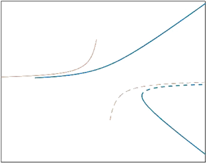
 $\pm \chi /16$, represents the approach to (a perturbed solution of) the spontaneous motion observed in Michelin et al. (Reference Michelin, Lauga and Bartolo2013), see figure 2. In that same limit, the branch (8.2) approaches the perturbed stationary state, namely the global solution (6.1). Since the stationary solution of the unforced problem is unstable for
 $\alpha >4$, it follows that the branch (8.2) is unstable. For
 $\chi >8\sqrt {2}$, the stable branches of the local solution are therefore given by (8.1) and (8.3). The above discussion also implies that the perturbed global solution (6.1) is unstable for
 $\alpha >4$. The preceding conclusions are illustrated in figure 3, depicting the variation of the particle velocity (scaled by
 $\epsilon ^{1/2}$) as a function of
 $\chi$. It is remarkable that, for
 $\alpha >4$, a force in the positive
 $z$-direction may result in particle motion in the negative
 $z$-direction.
Particle velocity as a function of  $\alpha$. The symbols depict the numerically evaluated speed of the spontaneous motion in the unforced problem (Michelin et al. Reference Michelin, Lauga and Bartolo2013). The solid curve depicts the local approximation (6.5) with
 $\epsilon =10^{-4}$ and
 $W_{1/2}$ taken as the positive local branch (8.1).

Particle velocity (scaled by  $\epsilon ^{1/2}$) as a function of
 $\chi$. The thick curves depict the local solution: the stable branches (8.1) and (8.3) are indicated by solid curves, while the unstable branch (8.2) is indicated by a dashed curve. The thin curves depict the global perturbation (6.1) to the stationary state, calculated for
 $\epsilon =0.01$: the stable branch (
 $\alpha <4$) is indicated by a solid curve, while the unstable branch (
 $\alpha >4$) is indicated by a dashed curve.

8.2. The direction of motion
In the global analysis, particle motion appeared only at the  $O(\epsilon )$ analysis. The flow at this asymptotic order was triggered by an external force in the
 $z$-direction (see (4.12)), and the solution was unique. It was then evident that particle motion must take place in the
 $z$-direction, and that the flow and solute transport must be symmetric about the
 $z$-axis. These symmetry assumptions were actually taken for granted in the problem formulation (§ 3).
The situation is quite different in the local analysis. Here, the  $O(\epsilon ^{1/2})$ problem is homogeneous, and may admit multiple solutions. In fact, since the external force appears only at the following
 $O(\epsilon )$ problem, there is no preference to the
 $z$-direction over any other direction. In principle, one might have sought a particle motion at
 $O(\epsilon ^{1/2})$ in any arbitrary direction. The
 $z$-direction would then enter the analysis only at the
 $O(\epsilon )$ problem.
We claim that such a generalised approach would furnish a steady-state solution corresponding to particle motion in the  $z$-direction. The reason has to do with the need for the (vectorial) particle velocity obtained by the local analysis to match the (vectorial) particle velocity obtained by the global analysis. The latter is fixed at the
 $z$-direction (both below and above the critical value
 $\alpha =4$). This argument justifies the compact analysis used herein.
Since the unforced problem is known to admit spontaneous particle motion in an arbitrary direction, it may appear strange that a small forcing would change that arbitrariness. To illustrate such dramatic effect of a small forcing, it is convenient to employ the following toy model governing the dynamics of a time-dependent vector  $\boldsymbol {v}$:
 \begin{equation} \frac{{\rm d} {\boldsymbol{v}}}{{\rm d} {t}} = \sigma \boldsymbol{v} - |\boldsymbol{v}|\boldsymbol{v} + \varDelta \hat{\boldsymbol{e}}_z, \end{equation}
wherein  $\sigma$ is a bifurcation parameter and
 $\varDelta$ is an ‘imperfection’ parameter. For the unforced problem, where
 $\varDelta =0$, we find two types of fixed points: the trivial solution
 $\boldsymbol {v}=\boldsymbol {0}$ and, for
 $\sigma >0$, a family of non-trivial solutions, where the direction of
 $\boldsymbol {v}$ is arbitrary with
 $|\boldsymbol {v}|=\sigma$. The latter type is akin to the steady spontaneous particle motion of Michelin et al. (Reference Michelin, Lauga and Bartolo2013), especially near the bifurcation at
 $\alpha =4$ where the speed grows in proportion to
 $\alpha -4$. In the forced problem, however, where
 $\varDelta \ne 0$, both the
 $x$- and
 $y$-components of the fixed point must vanish in order to avoid contradiction. It follows that
 $\boldsymbol {v}$ is parallel to
 $\hat {\boldsymbol {e}}_z$, say
 $\boldsymbol {v}=s\hat {\boldsymbol {e}}_z$, and the imperfect bifurcation is governed by the equation
 $(\sigma -|s|)s=-\varDelta$, which is analogous to (7.27). The manner by which the parameter
 $\varDelta$ changes the fixed points dramatically becomes evident once the system is considered dynamically. The ‘perfect’ solutions satisfying
 $|\boldsymbol {v}|=\sigma$, with the direction of
 $\boldsymbol {v}$ being arbitrary, are then quite relevant – they are nearly fixed points; they drift to the exact
 $z$-directed fixed points exceedingly slowly as
 $\varDelta \to 0$.
We anticipate that a similar mechanism would appear in the physical problem we consider had we addressed the unsteady version of the local problem. At time zero, we would have observed an  $O(\epsilon ^{1/2})$ particle motion at an arbitrary direction, corresponding to the spontaneous motion of Michelin et al. (Reference Michelin, Lauga and Bartolo2013). That motion, however, would violate at
 $O(\epsilon )$ the conditions of a steady solution, and it would accordingly evolve with time. Only at long times would the particle velocity approach a stable solution – either (8.1) or (8.3).
9. Concluding remarks
We have analysed the steady states of motion of an isotropic active particle that is subjected to a constant and uniform external force field. To facilitate analytical treatment of the problem, we have assumed that the mechanical velocity scale  $\mathcal {W}$ associated with that field is small compared with the natural diffusio-osmotic scale
 $\mathcal {U}$. The intrinsic Péclet number
 $\alpha$ based on the latter velocity scale was allowed to attain arbitrary order-unity values.
In the absence of the external force field, there is always a trivial steady state where both the particle and fluid are at rest. In the first part of our analysis, we have studied the linear perturbation from that stationary state produced by the weak external force field. In this linearisation scheme, the solute cloud in the neighbourhood of the particle remains approximately spherically symmetric and the particle and fluid velocities are in proportion to the external force. At linear order, solute advection disturbs the spherical symmetry of the solute cloud, resulting in a diffusio-osmotic flow. For  $\alpha =O(1)$, that flow is comparable to the mechanical velocity scale
 $\mathcal {W}$ associated with the external force; it therefore significantly affects particle mobility, while giving rise to a feedback loop where the diffusio-osmotic flow, engendered by the deformation of the solute cloud, affects that same deformation by contributing to the total flow field advecting the solute. Our analysis furnishes a closed-form expression for the linearised mobility, which differs significantly from the classical Stokes mobility for a chemically inert particle. This expression depends on
 $\alpha$ and the product of signs
 $AM$, which effectively determines whether the diffusio-osmotic feedback is positive or negative. Thus, for
 $AM<0$, diffusio-osmosis diminishes particle mobility relative to the case of an inert particle, for all
 $\alpha >0$. In contrast, for
 $AM>0$, the mobility is enhanced for
 $\alpha <4$ and reversed for
 $\alpha >4$; at
 $\alpha =4$, the linearised mobility diverges.
In hindsight, the failure of the above linearisation scheme at  $\alpha =4$ was to be expected given that the stationary base state is known to bifurcate at that value. Thus, in the unforced problem, a manifold of non-trivial steady states, associated with spontaneous motion in an arbitrary direction, emerges at the critical value
 $\alpha =4$, with the speed of spontaneous motion initially growing linearly with
 $\alpha -4$. Given this symmetry breaking, it is clear that the perturbation by the weak external force field must be non-uniform in
 $\alpha$. Accordingly, in the second part of our analysis, we have carried out a weakly nonlinear analysis in a distinguished local neighbourhood of
 $\alpha =4$. This analysis has furnished a closed-form description of the imperfect bifurcation linking the two branches of the linearly perturbed stationary state and the perturbed states of spontaneous motion. While the latter were not analysed in detail in this paper, we argue that, to leading order, these coincide with the unperturbed spontaneous-motion states only restricted to the directions parallel and antiparallel to the external force field.
This latter finding suggests that the symmetry breaking underpinning the spontaneous motion of isotropic active particles is structurally unstable, in the sense that weak perturbations may result in drastic changes to the set of permissible steady motions, both near and away from the bifurcation. In the present context, we conclude that even a weak force field would suffice to align the spontaneous motion of an isotropic active particle in a given direction. We expect, however, the dynamics of this alignment to become slower the weaker the perturbation. More generally, other forms of perturbations may also result in similarly dramatic consequences. One alternative forcing is an ambient flow. In that context, the simplest flow is probably a simple shear (Frankel & Acrivos Reference Frankel and Acrivos1968; Yariv & Kaynan Reference Yariv and Kaynan2017), but one may also consider more general linear flows (Batchelor Reference Batchelor1979; Yariv Reference Yariv2019). Rather than external forcing, one could also consider perturbations owing to a slight asymmetry in the particle geometry or surface composition, or weak interactions with distant particles and boundaries. We note that axisymmetric (Lippera et al. Reference Lippera, Morozov, Benzaquen and Michelin2020c; Lippera, Benzaquen & Michelin Reference Lippera, Benzaquen and Michelin2020b) and planar (Lippera, Benzaquen & Michelin Reference Lippera, Benzaquen and Michelin2020a) interactions have recently been considered in the different physical context of active droplets, discussed in § 1. These studies also employed a weakly nonlinear analysis near the critical Péclet number (Lippera et al. Reference Lippera, Morozov, Benzaquen and Michelin2020c).
Lastly, we note that a by-product of our perturbative analysis is an alternative prediction of the critical value  $\alpha =4$ at which the unforced problem undergoes a bifurcation. Originally, this value was obtained through a linear-stability analysis, which showed that beyond that value the stationary state is unstable (Michelin et al. Reference Michelin, Lauga and Bartolo2013). This is consistent with the fact that, in our analysis of the forced problem, the linearised scheme collapses at that value owing to the existence there of a non-trivial solution to the homogeneous problem, i.e. the one obtained by disregarding the external-force constraint. Heuristically, the feedback loop coupling solute transport and diffusio-osmosis becomes self-sustaining at this
 $\alpha$-value. Furthermore, our local analysis near the critical value has revealed certain features of the bifurcation that were not directly observed in the linear-stability analysis of the unforced problem. One such feature follows from the need of the bifurcation branches (8.1) and (8.3) to match the local behaviour of the spontaneous-motion modes as
 $\alpha \searrow 4$: this matching requirement implies the slope
 $1/16$ for the spontaneous velocity as a function of
 $\alpha -4$.
Acknowledgements
We are grateful to S. Michelin for providing us the numerical data underlying figure 3 of Michelin et al. (Reference Michelin, Lauga and Bartolo2013).
Funding
E.Y. was supported by the United States – Israel Binational Science Foundation (Grant No. 2019642).
Declaration of interests
The authors report no conflict of interest.



