1 Introduction
Shear layer flow may be the most common flow that arises in virtually every application, including jets, flow over a cavity, a separated boundary layer over an aerodynamic body, and merging of two streams behind the trailing edge of an airfoil. Accordingly, active control of shear layer flows has been a major area of interest for the community. Early efforts on control of shear layers arising from separated flows have been summarized by Gad-el Hak & Bushnell (Reference Gad-el Hak and Bushnell1991). For jet flows, Wiltse & Glezer (Reference Wiltse and Glezer1998) examined the use of dissipative-range forcing with piezoelectric actuators and found that the high-frequency actuation is able to enhance the turbulent energy cascade and increase the dissipation of turbulent kinetic energy. Later, Seifert & Pack (Reference Seifert and Pack1999) examined the effect of synthetic jet actuation for flow control of a separated flow over a NACA 0015 airfoil and found that the actuation is able to delay stall and improve post-stall aerodynamic performance. With plasma actuators, these control effects were also observed by Post & Corke (Reference Post and Corke2004) on the same airfoil. The uses of plasma actuators on other shear layer set-ups have been continuing to attract research interest (Samimy et al. Reference Samimy, Kim, Kastner, Adamovich and Utkin2007; Corke, He & Patel Reference Corke, He and Patel2009; Akins, Singh & Little Reference Akins, Singh and Little2015). Synthetic-jet-based flow control of a shear layer that forms in a separated flow over a wall-mounted hump was studied by Greenblatt et al. (Reference Greenblatt, Paschal, Yao and Harris2006), who showed that control input from the jet is able to change the generation rate of turbulent kinetic energy along the shear layer. For shear layers in cavity flows, Cattafesta et al. (Reference Cattafesta, Song, Williams, Rowley and Alvi2008) summarized flow control attempts using a number of modern actuators. Flow over a backward-facing step is also a canonical problem set-up where a shear layer is formed, and was chosen by Vukasinovic, Rusak & Glezer (Reference Vukasinovic, Rusak and Glezer2010) to investigate high-frequency actuation effects from a spanwise arrangement of synthetic jets. While the above studies do not encompass all studies to date, they show the breadth of active control techniques being applied to shear layers that arise from a range of flows.
Among the aforementioned flows, the free shear layer formed by the mixing of two streams with different velocities is considered especially to be the canonical configuration for shear layer flows. Studies on the characteristics of free shear layers date back to the seminal work of Brown & Roshko (Reference Brown and Roshko1974), where it was shown that the large spanwise roll-up coherent structures forming behind the trailing edge of a splitter plate serve as the main driving force for mixing of two streams and induce the entrainment that feeds fluid from two streams to the mixing region. Along with their work, Winant & Browand (Reference Winant and Browand1974) and Ho & Huang (Reference Ho and Huang1982) have attributed the initial shear layer roll-up to the fundamental instability waves, whereas their subharmonic instability accounts for the vortex merging downstream. These findings were later extended to compressible flow by Elliott & Samimy (Reference Elliott and Samimy1990) and Clemens & Mungal (Reference Clemens and Mungal1995).
As a fundamental study on the free shear layer instabilities, Ho & Huang (Reference Ho and Huang1982) introduced (non-local) subharmonic velocity disturbances in the entire free stream. Bechert & Stahl (Reference Bechert and Stahl1988) found that the external acoustic excitation is also able to trigger the instability wave in the shear layer. While leveraging of flow instabilities is a general strategy for flow control, the introduction of control inputs in a limited local region may be a more practical approach than the introduction of control inputs externally. On the other hand, Barone & Lele (Reference Barone and Lele2005) studied the receptivity of the shear layer behind a finite-thickness splitter plate to various types of disturbances by performing adjoint simulations. Temperature disturbance is among these disturbances, and the shear layer is found to be receptive to such a perturbation. However, studies on the excitation of a shear layer instability by directly manipulating the local temperature are limited in the literature. For these two reasons, the use of a localized thermal forcing input for flow control on a free shear layer draws our interest to the present study.
The objective of this study is to assess the effectiveness of the use of local periodic heating for modification of the early evolution of a free shear layer. The two-dimensional Navier–Stokes equations are numerically solved to simulate a spatially developing shear layer downstream of a finite-thickness splitter plate, with local periodic heating introduced at the trailing edge. As has been pointed out by Crighton (Reference Crighton1985) and Bechert (Reference Bechert1988), active control of a shear layer by the introduction of control inputs downstream of the trailing edge appears to be ineffective, but control via manipulation of the instabilities at the onset of a shear layer can be effective. A slight perturbation during the genesis of a shear layer can lead to an overall change in the flow physics downstream, because its instability characteristics determine which existing disturbances can be amplified. Nonlinear effects take place when the disturbance becomes large in magnitude and transfers energy among modes while creating new ones, which drives the evolution of the flow. Thus, the focusing of forcing input to the origin of a shear layer is favourable for flow control since the input can leverage the flow instabilities to grow and alter the flow behaviour downstream.
Our fundamental study on the use of local periodic heating as a forcing input to modify the spatial evolution of a shear layer is inspired by the development in thermophones and nanosecond pulse-driven dielectric barrier discharge (ns-DBD) actuators. Regarding the former, the thermophone is a sound generation technique discovered by Arnold & Crandall (Reference Arnold and Crandall1917). With the application of alternating current (AC) over a platinum film, they found that the Joule heating on the film periodically increases the surrounding fluid temperature and leads to local pressure fluctuations at double the frequency of the alternating current. This thermophone technique has not been widely utilized in the past due to the relatively large power required for a desired surface pressure disturbance level. In recent years, however, this drawback has been overcome by the use of graphene- and carbon-nanotube-based membranes for thermophones. Compared with traditional metal membranes, carbon-based membranes can be fabricated to be extremely thin, usually around
 $O(10^{-5})$
mm (Tian et al.
Reference Tian, Ren, Xie, Wang, Zhou, Feng, Fu, Yang, Peng and Wang2011), such that their heat capacity per unit area (HCPUA) is at least two orders of magnitude lower than that of metal films. Since the output power of the pressure disturbance delivered to the surrounding flow field is inversely proportional to the material HCPUA, the use of carbon-based membranes dramatically enhances the device efficiency. The operating frequency is also extended in range (
 $20$
–
 $50$
kHz) with these membranes (Tian et al.
Reference Tian, Ren, Xie, Wang, Zhou, Feng, Fu, Yang, Peng and Wang2011; Bin, Oates & Taira Reference Bin, Oates and Taira2015). Considering the thermophone as a new candidate for flow control actuators, the broadened range of its operating frequency is able to encompass those of many flow control applications.
On the other hand, the use of ns-DBD actuators for flow control has also become widespread in recent years (Little et al. Reference Little, Takashima, Nishihara, Adamovich and Samimy2012; Lehmann, Akins & Little Reference Lehmann, Akins and Little2014). The control mechanism of ns-DBD plasma actuation is believed to primarily rely on the deposition of thermal energy (Nudnova, Aleksandrov & Starikovskii Reference Nudnova, Aleksandrov and Starikovskii2010; Adamovich et al. Reference Adamovich, Little, Nishihara, Takashima and Samimy2012), in contrast to alternating current driven dielectric barrier discharge (ac-DBD) actuators which employ an electrohydrodynamic effect to introduce momentum perturbation (Abe et al. Reference Abe, Takizawa, Sato and Kimura2008; Corke, Enloe & Wilkinson Reference Corke, Enloe and Wilkinson2010). Numerous studies have reported a rapid heating effect near a pulse-driven plasma actuator and attributed the kinetic mechanism of the localized heating to the energy transfer to molecular translational/rotational modes on a sub-microsecond time scale (Aleksandrov et al. Reference Aleksandrov, Kindysheva, Nudnova and Starikovskiy2010; Popov Reference Popov2011). For both thermophone and ns-DBD actuators, their energy-flux-based actuators rely on no mechanical moving parts. Moreover, their sheet-like arrangement facilitates surface-compliant installation without occupying any internal space or adding significant weight. This advantage in installation allows them to be mounted on virtually any surface, and extends their potential uses for flow control on applications including rotorcraft blades and small-scale unmanned air vehicle wings.
In this study, we numerically examine the capability of this thermal-energy-flux-based actuation for flow control on a canonical free shear layer flow. In what follows, we describe the problem and discuss the computational set-up in § 2. Two boundary conditions for modelling local periodic heating are presented in § 2.3. Two-dimensional baseline shear layers are characterized in § 3. In § 4, the underlying mechanism by which thermal actuation can introduce perturbations to the flow field and alter the characteristics of the downstream shear layer is revealed by examining the near-field effect of the actuator. The flow control effect by local periodic heating on the downstream shear layer is discussed in detail in § 5. We conclude this study in § 6 by offering summarizing remarks.
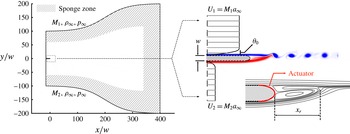
Computational set-up with a spatially developing shear layer downstream of a splitter plate. Two streams at free-stream Mach numbers of
 $M_{1}=0.4$
(top) and
 $M_{2}=0.1$
(bottom) enter the computational domain from the inlet boundary (
 $x/w=-15$
) on the left. A sponge zone is provided in the shaded region of the computational domain. A no-slip adiabatic boundary condition is imposed over the surface of the splitter plate. For forced flow, periodic heating is introduced from the actuator placed at the elliptic trailing edge by specifying an oscillatory heat flux boundary condition at a frequency
 $f^{+}$
.

2 Computational set-up
2.1 Problem description
We consider a two-dimensional free shear layer as a model problem to examine the effectiveness of thermal actuation. Two incoming streams at velocities
 $U_{1}$
and
 $U_{2}$
, initially separated by a splitter plate, at Mach numbers of
 $M_{1}=U_{1}/a_{\infty }=0.4$
(top) and
 $M_{2}=U_{2}/a_{\infty }=0.1$
(bottom) with the same free-stream acoustic speed,
 $a_{\infty }$
, and pressure,
 $p_{\infty }$
, form a spatially developing shear layer from the trailing edge, as illustrated in figure 1. Following the definition by Papamoschou & Roshko (Reference Papamoschou and Roshko1988), the mean convective Mach number for the shear layer is
 $M_{c}=(U_{1}-U_{2})/(2a_{\infty })=0.15$
, with the density ratio
 $\unicode[STIX]{x1D70C}_{1}/\unicode[STIX]{x1D70C}_{2}$
being unity (
 $\unicode[STIX]{x1D70C}_{1}=\unicode[STIX]{x1D70C}_{2}=\unicode[STIX]{x1D70C}_{\infty }$
). The plate-thickness-based Reynolds number,
 $Re_{w}\equiv \unicode[STIX]{x1D70C}_{\infty }\bar{U}w/\unicode[STIX]{x1D707}_{\infty }$
, is set to
 $2500$
, where
 $\bar{U}=(U_{1}+U_{2})/2$
is the convection velocity,
 $w$
is the plate thickness and
 $\unicode[STIX]{x1D707}_{\infty }$
is the free-stream dynamic viscosity. The boundary layers on both sides of the plate are prescribed with the same momentum thickness,
 $\unicode[STIX]{x1D703}_{0}$
, which is chosen to be
 $5\,\%$
,
 $10\,\%$
and
 $25\,\%$
of the splitter plate thickness,
 $w$
, causing the momentum-thickness-based Reynolds number
 $Re_{\unicode[STIX]{x1D703}_{0}}\equiv \unicode[STIX]{x1D70C}_{\infty }\bar{U}\unicode[STIX]{x1D703}_{0}/\unicode[STIX]{x1D707}_{\infty }$
to range from
 $125$
to
 $625$
.
2.2 Computational approach
The governing equations for the free shear layer are the compressible Navier–Stokes equations,
 $$\begin{eqnarray}\displaystyle & \displaystyle \frac{\unicode[STIX]{x2202}\tilde{\unicode[STIX]{x1D70C}}}{\unicode[STIX]{x2202}\tilde{t}}+\frac{\unicode[STIX]{x2202}}{\unicode[STIX]{x2202}\tilde{x}_{j}}(\tilde{\unicode[STIX]{x1D70C}}\tilde{u} _{j})=0, & \displaystyle\end{eqnarray}$$
 $$\begin{eqnarray}\displaystyle & \displaystyle \frac{\unicode[STIX]{x2202}}{\unicode[STIX]{x2202}\tilde{t}}(\tilde{\unicode[STIX]{x1D70C}}\tilde{u} _{i})+\frac{\unicode[STIX]{x2202}}{\unicode[STIX]{x2202}\tilde{x}_{j}}(\tilde{\unicode[STIX]{x1D70C}}\tilde{u} _{i}\tilde{u} _{j})=-\frac{\unicode[STIX]{x2202}}{\unicode[STIX]{x2202}\tilde{x}_{j}}(\tilde{p}\unicode[STIX]{x1D6FF}_{ij})+\frac{1}{Re}\frac{\unicode[STIX]{x2202}}{\unicode[STIX]{x2202}\tilde{x}_{j}}\left(\frac{\unicode[STIX]{x2202}\tilde{u} _{i}}{\unicode[STIX]{x2202}\tilde{x}_{j}}+\frac{\unicode[STIX]{x2202}\tilde{u} _{j}}{\unicode[STIX]{x2202}\tilde{x_{i}}}-\frac{2}{3}\frac{\unicode[STIX]{x2202}\tilde{u} _{k}}{\unicode[STIX]{x2202}\tilde{x_{k}}}\unicode[STIX]{x1D6FF}_{ij}\right), & \displaystyle\end{eqnarray}$$
 $$\begin{eqnarray}\displaystyle & \displaystyle \frac{\unicode[STIX]{x2202}\tilde{e}}{\unicode[STIX]{x2202}\tilde{t}}+\frac{\unicode[STIX]{x2202}}{\unicode[STIX]{x2202}\tilde{x}_{j}}[(\tilde{e}+\tilde{p})\tilde{u} _{j}]=\frac{1}{Re}\frac{\unicode[STIX]{x2202}}{\unicode[STIX]{x2202}\tilde{x}_{j}}\left[\tilde{u} _{i}\left(\frac{\unicode[STIX]{x2202}\tilde{u} _{i}}{\unicode[STIX]{x2202}\tilde{x}_{j}}+\frac{\unicode[STIX]{x2202}\tilde{u} _{j}}{\unicode[STIX]{x2202}\tilde{x_{i}}}-\frac{2}{3}\frac{\unicode[STIX]{x2202}\tilde{u} _{k}}{\unicode[STIX]{x2202}\tilde{x_{k}}}\unicode[STIX]{x1D6FF}_{ij}\right)\right]+\frac{1}{RePr}\frac{\unicode[STIX]{x2202}^{2}\tilde{T}}{\unicode[STIX]{x2202}\tilde{x_{k}}\unicode[STIX]{x2202}\tilde{x_{k}}},\quad & \displaystyle\end{eqnarray}$$
with the equation of state for ideal gas,
 $$\begin{eqnarray}\tilde{p}=\frac{\tilde{\unicode[STIX]{x1D70C}}\tilde{T}}{\unicode[STIX]{x1D6FE}},\end{eqnarray}$$
where
 $\unicode[STIX]{x1D6FE}$
is the specific heat ratio. The non-dimensional variables in (2.1)–(2.4) are the spatial coordinate
 $\tilde{x}_{i}$
, time
 $\tilde{t}$
, density
 $\tilde{\unicode[STIX]{x1D70C}}$
, velocity
 $\tilde{u} _{i}$
, pressure
 $\tilde{p}$
, energy
 $\tilde{e}$
and temperature
 $\tilde{T}$
according to the non-dimensionalization of
 $$\begin{eqnarray}\displaystyle \left.\begin{array}{@{}c@{}}\displaystyle \tilde{\unicode[STIX]{x1D70C}}=\frac{\unicode[STIX]{x1D70C}}{\unicode[STIX]{x1D70C}_{\infty }},\quad \tilde{p}=\frac{p}{\unicode[STIX]{x1D70C}_{\infty }a_{\infty }^{2}},\quad \tilde{T}=\frac{T}{T_{\infty }},\quad \tilde{e}=\frac{e}{\unicode[STIX]{x1D70C}_{\infty }a_{\infty }^{2}},\\ \displaystyle \tilde{u} _{i}=\frac{u_{i}}{a_{\infty }},\quad \tilde{x}_{i}=\frac{x_{i}}{w},\quad \tilde{t}=\frac{ta_{\infty }}{w}.\end{array}\right\} & & \displaystyle\end{eqnarray}$$
We note that the shear layer roll-up wavelength,
 $\unicode[STIX]{x1D706}_{n}$
, may also be used for the non-dimensionalization of the spatial coordinate
 $x_{i}$
in order to provide fair comparisons between different values of
 $\unicode[STIX]{x1D703}_{0}$
. In this paper, it will be clearly stated which length scale is being used for non-dimensionalization. The dimensionless parameters appearing in the governing equations are the acoustic Reynolds number and Prandtl number, given by
 $$\begin{eqnarray}Re\equiv \frac{\unicode[STIX]{x1D70C}_{\infty }a_{\infty }w}{\unicode[STIX]{x1D707}_{\infty }}\quad \text{and}\quad Pr\equiv \frac{\unicode[STIX]{x1D707}_{\infty }}{\unicode[STIX]{x1D70C}_{\infty }\unicode[STIX]{x1D6FC}_{\infty }},\end{eqnarray}$$
where
 $\unicode[STIX]{x1D6FC}_{\infty }$
is the free-stream thermal diffusivity.
To simulate the flow, we consider the two-dimensional set of equations and use the compressible flow solver CharLES (Khalighi et al.
Reference Khalighi, Ham, Moin, Lele, Schlinker, Reba and Simonich2011a
,Reference Khalighi, Nichols, Ham, Lele and Moin
b
; Brès et al.
Reference Brès, Ham, Nichols and Lele2017), which utilizes a second-order-accurate finite-volume method and a third-order Runge–Kutta scheme for time stepping. We use
 $\unicode[STIX]{x1D6FE}=1.4$
,
 $Re=10\,000$
and
 $Pr=0.7$
in the present study. These values are representative of standard air. The temperature-varying dynamic viscosity,
 $\unicode[STIX]{x1D707}(T)$
, is evaluated by a power law as
 $\unicode[STIX]{x1D707}=\unicode[STIX]{x1D707}_{\infty }(T/T_{\infty })^{0.76}$
(see Garnier, Adams & Sagaut Reference Garnier, Adams and Sagaut2009). The power law models the dynamic viscosity variation well for standard air in the range
 $T/T_{\infty }\in [0.5,1.7]$
. This range is suitable for the current study with local thermal inputs, where we observe that the temperature fluctuation is within
 $22\,\%$
about
 $T_{\infty }$
.
The computational domain, as illustrated in the left part of figure 1, has a streamwise extent of
 $x/w\in [-15,400]$
and a maximum vertical extent of
 $y/w\in [-200,200]$
, similar to the domain set-up used by Sharma, Bhaskaran & Lele (Reference Sharma, Bhaskaran and Lele2011). The splitter plate has an elliptic trailing edge with an eccentricity of
 $0.866$
, with its tip positioned at the origin,
 $x/w=y/w=0$
. The domain is discretized with a structured body-fitted mesh around the splitter plate. The near-wall resolution is
 $\unicode[STIX]{x0394}y^{+}\equiv \unicode[STIX]{x0394}yu^{\ast }/\unicode[STIX]{x1D708}_{\infty }=0.25$
(see Choi & Moin Reference Choi and Moin2012), where
 $u^{\ast }=\sqrt{\unicode[STIX]{x1D70F}_{0}/\unicode[STIX]{x1D70C}_{\infty }}$
is the wall shear velocity and
 $\unicode[STIX]{x1D70F}_{0}$
is the wall shear stress. To resolve the interaction between the shear layer and the localized periodic heat forcing, the wall-normal grid stretching rate is limited such that the
 $\unicode[STIX]{x0394}y^{+}$
only reaches a maximum of
 $1.25$
within
 $50w$
from the wall. The overall grid size is approximately
 $4.4\times 10^{5}$
. The direct numerical simulation (DNS) results from this mesh were verified by comparing the flow field with that from a finer mesh, where the grid was refined in the sheared region and had a size of
 $6.8\times 10^{5}$
grid points. No noticeable differences were found in the results from these two meshes.
Two streams are introduced to the computational domain from the inlet boundary (left) using a Blasius boundary layer velocity profile. Their density profiles are computed using the Crocco–Busemann relation, with the same far-field temperature and pressure. A sponge zone is applied along the top, bottom and outlet (right) boundaries to damp out existing acoustic waves and vortical structures (Freund Reference Freund1997). The target states of the sponge zone at the top and bottom boundaries are set to
 $[U_{1},\unicode[STIX]{x1D70C}_{\infty },p_{\infty }]$
and
 $[U_{2},\unicode[STIX]{x1D70C}_{\infty },p_{\infty }]$
respectively. At the outlet, the time-average flow is set to be the target state of the sponge zone.
In this study, the effects of momentum thickness, the forcing frequency and the amplitude are examined in the context of modifying the characteristics of the shear layer. The flow control set-up using local periodic heating and the associated input parameters are discussed below.
2.3 Local periodic heating
The thermal actuator model is implemented in the numerical simulations through a boundary condition. Over the elliptic trailing edge of the splitter plate, an oscillatory energy-flux (unsteady Neumann) boundary condition that introduces local periodic heating is prescribed to the energy equation (2.3), along with a no-slip boundary condition for the momentum equation (2.2). In the present study, we consider two forms of periodic heating. First, we consider a temporally oscillatory heat flux with zero mean as
 $$\begin{eqnarray}\dot{q}=\hat{q}\sin (2\unicode[STIX]{x03C0}f^{+}t)\cos \left(\frac{\unicode[STIX]{x03C0}}{w}y\right),\quad |y|<\frac{1}{2}w,\end{eqnarray}$$
where the net heating input to the local fluid is zero over the forcing period. We also consider another forcing input
 $\dot{q}^{p}$
which introduces a positive direct current (DC) offset to the expression of
 $\dot{q}$
in (2.7) such that the heat flux is always positive over the duty cycle,
 $$\begin{eqnarray}\dot{q}^{p}=\hat{q}[1+\sin (2\unicode[STIX]{x03C0}f^{+}t)]\cos \left(\frac{\unicode[STIX]{x03C0}}{w}y\right),\quad |y|<\frac{1}{2}w.\end{eqnarray}$$
In the expressions for
 $\dot{q}$
and
 $\dot{q}^{p}$
,
 $f^{+}$
and
 $\hat{q}$
denote the forcing frequency and amplitude respectively. For each choice of
 $\unicode[STIX]{x1D703}_{0}/w$
, the forcing frequency,
 $f^{+}$
, is normalized by the corresponding baseline shear layer roll-up frequency,
 $f_{n}$
, and is varied from
 $f^{+}/f_{n}=0.500$
to
 $1.25$
, over which we observe forcing effects. Since the heat flux amplitude,
 $\hat{q}$
, accounts for the forcing power that is introduced to the shear layer flow, we normalize the total heating power from the trailing edge by the characteristic kinetic energy flux across the momentum thickness as
 $$\begin{eqnarray}E^{+}=\frac{Q}{\frac{1}{2}\unicode[STIX]{x1D70C}_{\infty }\bar{U}^{2}\cdot \unicode[STIX]{x1D703}_{0}\bar{U}},\end{eqnarray}$$
where
 $$\begin{eqnarray}Q=f^{+}\int _{0}^{1/f^{+}}\int _{|y|<w/2}|\dot{q}|\,\text{d}y\,\text{d}t\end{eqnarray}$$
is the cyclic average heating power introduced by the actuator. This normalization can account for the use of a higher forcing amplitude,
 $\hat{q}$
, for a greater initial momentum thickness,
 $\unicode[STIX]{x1D703}_{0}$
, for a fair comparison of forcing requirements across different values of
 $\unicode[STIX]{x1D703}_{0}$
, since a thicker shear layer is expected to necessitate a higher level of perturbation inputs to modify the shear layer. We parameterize the normalized forcing power in this study in the range of
 $E^{+}=0.296$
–
 $2.96$
. This value is of the same order of magnitude of those used in plasma-based flow control works (Samimy et al.
Reference Samimy, Kim, Kastner, Adamovich and Utkin2007; Corke et al.
Reference Corke, Enloe and Wilkinson2010; Sinha et al.
Reference Sinha, Alkandry, Kearney-Fischer, Samimy and Colonius2012; Akins et al.
Reference Akins, Singh and Little2015). We also note that the maximum temperature fluctuation observed over the surface of the actuator is within
 $22\,\%$
about the free-stream temperature with the use of the largest forcing amplitude,
 $E^{+}=2.96$
, in
 $\unicode[STIX]{x1D703}_{0}/w=0.25$
cases.
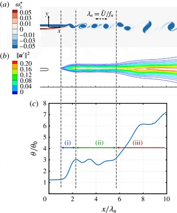
Baseline flow characterization for
 $\unicode[STIX]{x1D703}_{0}/w=0.1$
. (a) An instantaneous snapshot of the normalized spanwise vorticity
 $\unicode[STIX]{x1D714}_{z}^{\ast }=\unicode[STIX]{x1D714}_{z}\unicode[STIX]{x1D703}_{0}/\bar{U}$
. (b) Time-average velocity fluctuation magnitude
 $\Vert \boldsymbol{u}^{\prime }\Vert ^{2}=(u_{x}^{\prime 2}+u_{y}^{\prime 2})/\bar{U}^{2}$
. (c) Spatial growth of momentum thickness (
 $\unicode[STIX]{x1D703}/\unicode[STIX]{x1D703}_{0}$
). All share the same normalized streamwise coordinate,
 $x/\unicode[STIX]{x1D706}_{n}$
, where
 $\unicode[STIX]{x1D706}_{n}=\bar{U}/f_{n}$
is the baseline roll-up wavelength.

3 Baseline characterization
3.1 Shear layer characteristics
Let us first characterize the baseline flows at three momentum thicknesses specified at the inlet, namely
 $\unicode[STIX]{x1D703}_{0}/w=0.05$
,
 $0.1$
and
 $0.25$
. We focus our interest in the region within the streamwise extent of
 $10\unicode[STIX]{x1D706}_{n}$
, where
 $\unicode[STIX]{x1D706}_{n}=\bar{U}/f_{n}$
is the fundamental shear layer roll-up wavelength. Figure 2 shows a snapshot of the normalized instantaneous spanwise vorticity (a), the velocity fluctuation magnitude (b) and the momentum thickness profile (c) for the baseline flow with
 $\unicode[STIX]{x1D703}_{0}/w=0.1$
. In this work, the momentum thickness is computed using the density and streamwise velocity profiles in the shear layer as
 $$\begin{eqnarray}\unicode[STIX]{x1D703}(x)=\int _{-\infty }^{\infty }\frac{\overline{\unicode[STIX]{x1D70C}}(x,y)}{\unicode[STIX]{x1D70C}_{\infty }}\frac{[\overline{u}(x,y)-U_{2}][U_{1}-\overline{u}(x,y)]}{(U_{1}-U_{2})^{2}}\,\text{d}y,\end{eqnarray}$$
where the overbar denotes the time-averaged quantity based on the flow statistics collected over more than 200 roll-up periods. Comparing the spatial growth of momentum thickness with the instantaneous flow field, we classify the shear layer flow into three regions: (i) the shear layer roll-up region, where the momentum thickness exhibits the first rapid growth behind the trailing edge; (ii) the isolated vortex region, where each vortex formed remains compact as an individual and convects closely along the centreline; (iii) the vortex merging region, where the vortices start to deviate from the centreline while convecting downstream, as the initiation of the vortex merging process. This last region can be identified by the second rapid growth of the momentum thickness. These three regions can also be characterized by the streamwise change in velocity fluctuation magnitude. In regions (i) and (iii), the spatial extent and the magnitude of fluctuation are both increasing, but region (ii) shows no apparent changes in the growth of the momentum thickness except for a rippling variation in the momentum thickness profile. The cause of this ripple is that the orientation of the vortex evolves as the vortex convects downstream, which is discussed in appendix A. Later, in § 5, the forcing effect of periodic heating on the characteristics of these three regions is examined in further detail.
3.2 Influence of the splitter plate thickness
Due to the finite thickness of the splitter plate, a small recirculation region of length
 $x_{r}$
develops directly behind the blunt trailing edge of the splitter plate, as illustrated by the time-average streamlines in figure 1 (bottom right). This streamline pattern for two boundary layers merging behind the trailing edge of a finite-thickness splitter plate was also observed by Laizet, Lardeau & Lamballais (Reference Laizet, Lardeau and Lamballais2010) and Sharma et al. (Reference Sharma, Bhaskaran and Lele2011). The recirculation region can be viewed as a wake behind the finite-thickness splitter plate and results in a deficit in the profile streamwise velocity. In the theoretical study by Zhuang & Dimotakis (Reference Zhuang and Dimotakis1995), it was reported that a wake instability mode can be introduced to the shear layer which has a deficit in its streamwise velocity profile due to a wake component, and the growth rates of both the wake mode and the fundamental shear layer mode increase when the streamwise velocity profile has a greater wake deficit. Mehta (Reference Mehta1991) experimentally showed that the splitter plate wake plays a dominant role in the development of the shear layer. The wake increases the turbulence levels in the near-field and shortens the development distance to achieve self-similarity in shear layer profiles. Remarks by Mehta (Reference Mehta1991) on the lack of simple scaling for the shear layer with the presence of the wake also suggest that a nonlinear interaction is taking place between the wake and the shear layer. Laizet et al. (Reference Laizet, Lardeau and Lamballais2010) performed DNS of shear layers developing behind three different trailing edge geometries and reported that the presence of the wake can lead to different turbulent structures and shear layer spreading rates. We note, however, that no trace of von Kármán shedding is observed in the simulations considered here, in spite of the presence of the recirculation region.
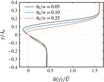
Time-average streamwise velocity profiles at
 $x/w=0.3$
over
 $y/\unicode[STIX]{x1D706}_{n}$
for three baseline cases, showing a stronger wake deficit for lower
 $\unicode[STIX]{x1D703}_{0}$
.

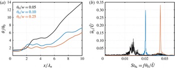
(a) Momentum thickness growth for baseline flows with
 $\unicode[STIX]{x1D703}_{0}/w=0.05$
,
 $0.1$
and
 $0.25$
. (b) Transverse velocity spectra for three baseline cases at
 $x/\unicode[STIX]{x1D706}_{n}=2.5$
. The shear layer roll-up frequency
 $f_{n}$
for each corresponding case is determined by the peak of its spectrum.

Baseline characteristics of the shear layer for different values of the momentum thickness
 $\unicode[STIX]{x1D703}_{0}/w$
: length of recirculation region
 $x_{r}/w$
; roll-up frequency
 $f_{n}w/\bar{U}$
; roll-up Strouhal number
 $St_{\unicode[STIX]{x1D703}_{0}}=f_{n}\unicode[STIX]{x1D703}_{0}/\bar{U}$
; roll-up wavelength
 $\unicode[STIX]{x1D706}_{n}/w$
.

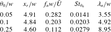
The lengths of the recirculation regions for each baseline case with varied momentum thickness
 $\unicode[STIX]{x1D703}_{0}/w$
are summarized in table 1, where the change in the wake length,
 $x_{r}/w$
, is limited to
 $6\,\%$
while
 $\unicode[STIX]{x1D703}_{0}/w$
is increased five times. At the streamwise station
 $x/w=3.0$
, the time-average streamwise velocity profile over the normalized transverse coordinate
 $y/\unicode[STIX]{x1D706}_{n}$
is presented in figure 3. It should be noted that the normalization of
 $y/\unicode[STIX]{x1D706}_{n}$
causes the velocity minimum to appear at different location for different choices of
 $\unicode[STIX]{x1D703}_{0}/w$
, since the value of
 $\unicode[STIX]{x1D706}_{n}$
is influenced by the value of
 $\unicode[STIX]{x1D703}_{0}/w$
. In figure 3, we observe that the wake deficit increases in both its transverse extent and its maximum velocity deficit for a thinner incoming boundary layer. In figure 4(a), we show the momentum thickness profile over the streamwise coordinate normalized by the corresponding roll-up wavelength for each case. As discussed previously using
 $\unicode[STIX]{x1D703}_{0}/w=0.1$
for the baseline characterization, the three-region growth patterns are also observed in the other two baseline cases. The initiation of merging takes place at
 $x/\unicode[STIX]{x1D706}_{n}\approx 6$
for all cases. However, thicker
 $\unicode[STIX]{x1D703}$
for the isolated vortex region and delayed roll-up are observed for thinner
 $\unicode[STIX]{x1D703}_{0}/w$
. These observations can be attributed to the stronger effect of the wake when
 $\unicode[STIX]{x1D703}_{0}$
is thinner. The effect of the plate wake can also be seen in the shear layer roll-up Strouhal number,
 $St_{\unicode[STIX]{x1D703}_{0}}=f_{n}\unicode[STIX]{x1D703}_{0}/\bar{U}$
, in table 1. We also note that the values of
 $St_{\unicode[STIX]{x1D703}_{0}}$
are lower than the prediction from linear instability theory (Monkewitz & Huerre Reference Monkewitz and Huerre1982; Ho & Huerre Reference Ho and Huerre1984),
 $St_{\unicode[STIX]{x1D703}_{0}}=0.032$
, in all baseline cases. This also suggests that the effective initial momentum thickness is greater than that on the high-speed side,
 $\unicode[STIX]{x1D703}_{0}$
, because of the presence of the wake. Therefore, for thinner
 $\unicode[STIX]{x1D703}_{0}$
, where the wake effect is more pronounced, a greater deviation of
 $St_{\unicode[STIX]{x1D703}_{0}}$
from
 $0.032$
is observed. The stronger wake effect on thin
 $\unicode[STIX]{x1D703}_{0}$
can also be inferred from figure 4(b), where the transverse velocity spectra at
 $x/\unicode[STIX]{x1D706}_{n}=2.5$
for three baseline cases are shown. The clean peaks in the cases of
 $\unicode[STIX]{x1D703}_{0}/w=0.1$
and
 $0.25$
suggest a synchronized shear layer roll-up and shedding, whereas the cause of the less prominent peak and broader frequency content in the case of
 $\unicode[STIX]{x1D703}_{0}/w=0.05$
can be attributed to the nonlinear interaction between the shear layer roll-up and the wake which redistributes the energy of the roll-up frequency to other nearby frequencies.
3.3 Local stability analysis
To determine regions with linear growth of the perturbations and predict the corresponding growth rate for the Kelvin–Helmholtz instability, local linear spatial stability analysis on the baseline flow is also performed in the onset region and the isolated vortex region of the shear layer. We compute the corresponding spatial growth rate at a specified perturbation frequency using the time-average density and streamwise velocity profiles as the base flow for the compressible Rayleigh equation (Sabatini & Bailly Reference Sabatini and Bailly2014).
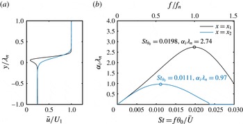
Figure 5 shows the stability analysis results for
 $\unicode[STIX]{x1D703}_{0}/w=0.1$
baseline flow. Time-average flow profiles at two streamwise stations (shown in a) are chosen about which to perform the instability analysis. The first station
 $x_{1}$
, corresponding to
 $(x_{1}-x_{r})/\unicode[STIX]{x1D706}_{n}=0.24$
or
 $x_{1}/\unicode[STIX]{x1D706}_{n}=1.22$
, is located slightly downstream of the recirculation region but upstream of the shear layer roll-up region. In figure 2, the station
 $x_{1}/\unicode[STIX]{x1D706}_{n}=1.22$
is located in the flat region before the first sudden growth of the momentum thickness. Similarly, we choose the second station
 $x_{2}$
, where
 $(x_{2}-x_{r})/\unicode[STIX]{x1D706}_{n}=3.1$
or
 $x_{2}/\unicode[STIX]{x1D706}_{n}=4.06$
, in the isolated vortex region indicated by the second flat region and before the second sudden growth. In figure 5, the most amplified frequencies and the corresponding spatial growth rates are
 $St_{\unicode[STIX]{x1D703}_{0}}=0.0198,\unicode[STIX]{x1D6FC}_{i}\unicode[STIX]{x1D706}_{n}=2.74$
and
 $St_{\unicode[STIX]{x1D703}_{0}}=0.0111,\unicode[STIX]{x1D6FC}_{i}\unicode[STIX]{x1D706}_{n}=0.97$
for stations
 $x=x_{1}$
and
 $x=x_{2}$
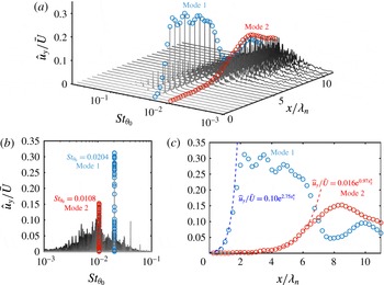
respectively. We compare these values with the results from DNS shown in figure 6. In figure 6(a), the spectra of transverse velocity are plotted over a series of streamwise locations. The symbol ○ (blue) (referred to as mode 1 hereafter) represents the first spatially amplified mode and ○ (red) (referred to as mode 2 hereafter) depicts the second mode. Their corresponding frequencies in terms of Strouhal numbers are
 $St_{\unicode[STIX]{x1D703}_{0}}=0.0204$
and
 $0.0108$
for modes 1 and 2 respectively, as captured in (b). Compared with the frequencies predicted by linear stability theory, the differences are only approximately
 $1.5\,\%$
and
 $3\,\%$
for modes 1 and 2 respectively. The spatial growth of the modal amplitude can be seen in figure 6(c). Additionally, in (c), the amplitude growth rates of modes 1 and 2 are fitted with exponential growth functions in the ranges
 $0\leqslant x/\unicode[STIX]{x1D706}_{n}\leqslant 1.6$
and
 $2.5\leqslant x/\unicode[STIX]{x1D706}_{n}\leqslant 5.5$
respectively. We also find that the growth rates
 $\unicode[STIX]{x1D6FC}_{i}\unicode[STIX]{x1D706}_{n}$
from the fitting differ by only
 $0.7\,\%$
and
 $2\,\%$
from the predictions of the linear theory for roll-up and merging modes respectively. The fitted function deviates from the simulation data ○ (blue) and ○ (red) past
 $x/\unicode[STIX]{x1D706}_{n}=1.5$
and
 $6.5$
respectively. These deviations are expected since, referring to figure 2, these two stations have already reached the vortex formation and merging regions where the momentum thickness exhibits a sudden streamwise growth and the parallel flow assumption is no longer valid.


Transverse velocity spectra over the centreline: (a) the spatial development of the spectra; (b) view from the amplitude–frequency plane; (c) streamwise profiles of modal amplitudes for the roll-up and merging modes with fitted exponential growth functions, where
 $x_{1}^{\ast }=(x-x_{1})/\unicode[STIX]{x1D706}_{n}$
and
 $x_{2}^{\ast }=(x-x_{2})/\unicode[STIX]{x1D706}_{n}$
. The frequencies and growth rates of modes 1 and 2 agree with the linear stability theory prediction in figure 5 with less than
 $3\,\%$
difference.

The agreement between the results from DNS and the linear stability analysis on the baseline flow provides deep insight into the growth of perturbations in the aforementioned regions. As we discuss later, the frequencies in the vicinity of that of mode 2 are also considered as candidates for the actuation frequency of the local periodic forcing in § 5. The growth rate prediction at the forcing frequency will also be compared with the forced cases later in discussions related to figures 10 and 14.
4 Thermal control mechanism
In this section, the local effects of periodic thermal forcing are studied to understand how the thermal perturbations give rise to hydrodynamic perturbations and modify the shear layer physics downstream. The local temperature fluctuation and surface pressure disturbance introduced by local periodic heating change the local vorticity flux through the solid boundary by changing either the surrounding fluid properties or the wall-tangential pressure gradient (Hornung Reference Hornung1989; Wu & Wu Reference Wu and Wu1993). The fluctuations in pressure and density in the vicinity of the actuator may also generate volumetric baroclinic vorticity,
 $(\unicode[STIX]{x1D735}\unicode[STIX]{x1D70C}\times \unicode[STIX]{x1D735}p)/\unicode[STIX]{x1D70C}^{2}$
. In this two-dimensional study, we evaluate the local wall-normal vorticity flux using (Wu & Wu Reference Wu and Wu1993)
 $$\begin{eqnarray}\unicode[STIX]{x1D70E}_{z}(s)=-\frac{1}{\unicode[STIX]{x1D70C}_{0}(s)}\{\hat{\boldsymbol{e}}_{n}(s)\boldsymbol{\cdot }\unicode[STIX]{x1D735}[\unicode[STIX]{x1D707}(s)\unicode[STIX]{x1D714}_{z}(s)]_{0}\},\end{eqnarray}$$
where
 $\unicode[STIX]{x1D707}$
and
 $\unicode[STIX]{x1D714}_{z}$
are the dynamic viscosity and spanwise vorticity respectively, subscript
 $0$
denotes the wall-adjacent quantities,
 $s$
is the spatial parameter describing the splitter plate surface and
 $\hat{\boldsymbol{e}}_{n}$
is the unit wall-normal vector. In two-dimensional Cartesian coordinates, the baroclinic torque generation is computed using
 $$\begin{eqnarray}B_{z}(x,y)=\frac{1}{\unicode[STIX]{x1D70C}^{2}}\left(\frac{\unicode[STIX]{x2202}\unicode[STIX]{x1D70C}}{\unicode[STIX]{x2202}x}\frac{\unicode[STIX]{x2202}p}{\unicode[STIX]{x2202}y}-\frac{\unicode[STIX]{x2202}\unicode[STIX]{x1D70C}}{\unicode[STIX]{x2202}y}\frac{\unicode[STIX]{x2202}p}{\unicode[STIX]{x2202}x}\right).\end{eqnarray}$$
These two quantities from the baseline and forced flows are examined below.
Without loss of generality, we consider the case with
 $\unicode[STIX]{x1D703}_{0}/w=0.1$
. The two quantities in (4.1) and (4.2) for the baseline and forced flows are examined to quantify their fluctuation magnitudes and frequencies. The forced and baseline computations are started at
 $tf_{n}=0$
from the same initial condition, which is associated with the instantaneous baseline flow with steady flow statistics. For the forced case, periodic heating at the trailing edge is turned on at
 $tf_{n}=0$
using (2.7) with
 $f^{+}/f_{n}=0.500$
and amplitude of
 $E^{+}=0.741$
. Flow statistics are collected over
 $tf_{n}\in [100,250]$
.
Fluctuation magnitude of spanwise vorticity flux over the plate surface,
 $\unicode[STIX]{x1D70E}_{z,rms}^{\ast }$
, and volumetric baroclinic torque generation rate,
 $B_{z,rms}^{\ast }$
, of the baseline (a) and forced (
 $f^{+}/f_{n}=0.500$
, b) flows. Both quantities exhibit higher levels of fluctuation in the controlled case.

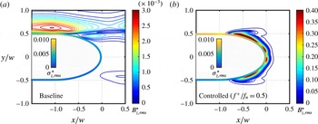
The change in these two quantities between the forced and baseline cases is shown in figure 7, where
 $\unicode[STIX]{x1D70E}_{z,rms}^{\ast }=\unicode[STIX]{x1D70E}_{z,rms}/\unicode[STIX]{x1D6FA}_{z}$
is the root-mean-square value of
 $\unicode[STIX]{x1D70E}_{z}$
, normalized by
 $\unicode[STIX]{x1D6FA}_{z}=\int _{y\in inlet}\unicode[STIX]{x1D714}_{z}\boldsymbol{u}\boldsymbol{\cdot }\hat{\boldsymbol{e}}_{n}\,\text{d}y$
, namely the total Euler flux of vorticity introduced by two inlet boundary layers. Similar normalization is used for
 $B_{z,rms}^{\ast }$
. We observe that both of these quantities exhibit higher fluctuation magnitudes in the thermally forced flow. Furthermore, we note that the maximum magnitude of
 $B_{z,rms}^{\ast }$
in the vicinity of the actuator is
 $O(10^{2})$
higher than that of the baseline flow. As reported by Cheung & Lele (Reference Cheung and Lele2009), the baroclinic vorticity generation plays an important role in governing shear layer dynamics, especially for subsonic shear layers. In their study, the order of magnitude difference between a heated (free-stream temperature ratio of
 $1.5$
) and an unheated (with the same free-stream temperature) shear layer is also of
 $O(10^{2})$
. The additional generation of baroclinic vorticity takes part in the vortex dynamics in the heated shear layer and leads to different behaviour from the unheated shear layer.
We compute the total vorticity flux over the trailing edge as
 $$\begin{eqnarray}{\mathcal{J}}_{z}=\int _{s\in tip}\unicode[STIX]{x1D70E}_{z}(s)\,\text{d}s\end{eqnarray}$$
and the total baroclinic generation near the trailing edge as
 $$\begin{eqnarray}{\mathcal{B}}_{z}=\int _{|\boldsymbol{r}|<2w}B_{z}(\boldsymbol{r})\,\text{d}v.\end{eqnarray}$$
The quantities
 ${\mathcal{J}}_{z}$
and
 ${\mathcal{B}}_{z}$
are normalized by
 $\unicode[STIX]{x1D6FA}_{z}$
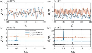
and plotted in figures 8(a,c) and 8(b,d) respectively, over the time and frequency domains. As observed from the frequency domain, both of these quantities peak at the forcing frequencies, suggesting that the fluctuations in
 ${\mathcal{J}}_{z}$
and
 ${\mathcal{B}}_{z}$
are indeed induced by the local periodic forcing.
(a,c) Total vorticity flux,
 ${\mathcal{J}}_{z}$
, over the trailing edge and (b,d) total volumetric baroclinic torque generation,
 ${\mathcal{B}}_{z}$
, near the trailing edge. The temporal oscillations and the frequency spectra are shown in (a,b) and (c,d) respectively. Measurements from the baseline and two forced (
 $f^{+}/f_{n}=0.500$
and
 $f^{+}/f_{n}=1.16$
) flows are presented. In the control cases, both
 $\widehat{J}_{z}/\unicode[STIX]{x1D6FA}_{z}$
and
 $\widehat{B}_{z}/\unicode[STIX]{x1D6FA}_{z}$
have a prominent peak at the forcing frequency. The spectra are shifted vertically for graphical clarity.

The present flow control technique utilizes local periodic heating as an energy-deposition-based forcing, which introduces additional generation of vorticity. As vorticity quantifies the rotation of fluid particles, we may also consider the present technique as a vorticity-based forcing, in contrast to other momentum-based flow control techniques such as synthetic jets (Glezer & Amitay Reference Glezer and Amitay2002). When the extra oscillatory vorticity is introduced to the shear layer at its onset, it can trigger the instability responsible for the shear layer roll-up, or modify the strength of each vortex formed from shear layer roll-up and change their interaction dynamics downstream.
5 Flow control effects on the shear layer
In this section, the influence of the forcing frequency (
 $f^{+}$
) and the forcing type (
 $\dot{q}$
and
 $\dot{q}^{p}$
) on the shear layer is examined. Each DNS is initialized with an instantaneous flow field from the baseline flow, with steady statistics based on at least
 $300$
fundamental roll-up periods. Forcing is turned on from this initial condition. Flow statistics for the controlled flows are collected after
 $100$
roll-up periods. The reported controlled flow spectrum and mean-flow-based momentum thickness are evaluated over at least another
 $200$
roll-up periods. We start the discussion with the use of
 $\dot{q}$
in §§ 5.1 and 5.2. Forcing with
 $\dot{q}^{p}$
, which is
 $\dot{q}$
with a positive DC offset, is examined in § 5.3.
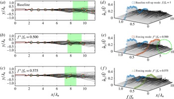
Vortex trajectories (a–c) and modal amplitude evolution (d–f) for
 $\unicode[STIX]{x1D703}_{0}/w=0.1$
. The merging location and its spatial variation are depicted by the green-shaded region (a–c) for each case. The forcing mode for
 $f^{+}/f_{n}=0.500$
maintains its high level of modal amplitude while marching downstream, and suppresses other lower-frequency modes from growing, as highlighted by the cleaner spectra in the green circled region.

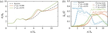
(a) Momentum thickness growth and (b) modal amplitude evolution for
 $\unicode[STIX]{x1D703}_{0}/w=0.1$
with forcing frequency close to the first subharmonic of
 $f_{n}$
.

5.1 Spreading enhancement (
 $f^{+}\approx 0.5f_{n}$
)

We examine the forcing effect when the actuation frequency is close to the first subharmonic of the roll-up frequency with the use of
 $\dot{q}$
. Two forcing frequencies are examined, namely
 $f^{+}/f_{n}=0.575$
and
 $0.500$
. The forcing frequency
 $f^{+}/f_{n}=0.575$
is selected for being close to the frequency of mode 2 found in figure 6. The exact first subharmonic
 $f^{+}/f_{n}=0.500$
is also chosen. For fair comparison, all cases presented in this section are based on the same forcing power of
 $E^{+}=0.741$
. In the discussion below, we first highlight the common forcing effects for these two forcing frequencies. We then discuss the differences between the two forced cases.
We start our detailed discussion on cases with
 $\unicode[STIX]{x1D703}_{0}/w=0.1$
. The baseline and forced flows are compared in figures 9 and 10. It is found that the forcing is able to change the vortex dynamics by encouraging the merging downstream while keeping the momentum thickness unchanged in the region dominated only by fundamental roll-up. We first track the centre of each individual vortex after roll-up using the
 $Q$
-criterion. By tracking all formed vortices over a time span of
 $100$
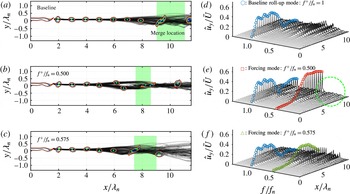
roll-up periods, we visualize the vortex trajectories by black transparent dots and the contour lines for a representative instantaneous spanwise vorticity field in figure 9(a–c). On observing the trajectories, it is clear that, as the vortices convect downstream, they spread away from the centreline (
 $y/\unicode[STIX]{x1D706}_{n}=0$
) earlier upstream in the forced flows compared with the baseline case. This deviation from the centreline serves as an initiation for the vortex merging process (Winant & Browand Reference Winant and Browand1974; Ho & Huang Reference Ho and Huang1982). While the vortex merging process takes place, the flow passes through a stage where a pair of vortices become vertically aligned, which then results in steep spatial growth of the momentum thickness. For example, the controlled case with
 $f^{+}/f_{n}=0.500$
shows the vertical alignment to take place at
 $x/\unicode[STIX]{x1D706}_{n}\approx 7$
. By observing the momentum thickness in figure 10(a), we find that this steep growth indeed corresponds to where the trajectories demonstrate deviation from the centreline for each case. With forcing at these two frequencies, the momentum thickness does not exhibit any change from that of the baseline until this second growth takes place farther upstream compared with the baseline.
A merging criterion is set up such that two vortices are considered to be merged if their instantaneous mutual distance is less than
 $0.2\unicode[STIX]{x1D706}_{n}$
. By setting this threshold, we show the average streamwise location along with the variation (standard deviation) in where merging takes place by the green-shaded regions for each case in figure 9(a–c). Again, by comparing the shaded regions from the forced cases with the baseline, it is found that the merging process completes upstream with reduced spatial variation. Observations made from the vortex tracking and the mean flow momentum thickness both enable us to draw the conclusion that the forcing is able to change the vortex dynamics by encouraging the merging downstream while keeping the momentum thickness unchanged in the region dominated only by fundamental roll-up.
Since the vortex merging process is dominated by the subharmonics of the roll-up frequency, we now examine the flow over the frequency domain and focus on low-frequency components with
 $f/f_{n}\leqslant 1$
. The transverse velocity spectra along the centreline are shown in figure 9(d–f) for each corresponding case in (a–c). On comparing the forced cases with the baseline case, we find that the forcing mode in each forced case is amplified downstream, which suggests that both control inputs (
 $f^{+}/f_{n}=0.500$
and
 $0.575$
) are efficiently leveraging the shear layer instability. Moreover, the growth rates of these two forcing modes are both well predicted by the local stability analysis, as previously depicted in figure 5. The energy distribution among the spectra does not show noticeable change from the baseline case until these two forcing modes start to be amplified at
 $x/\unicode[STIX]{x1D706}_{n}\approx 4$
, as shown in figure 9(d–f). As discussed in § 3.3, this streamwise station is in the isolated vortex region with linear perturbation growth. This location also corresponds to where the momentum thickness starts to depart from that of the baseline with forcing, as seen in figure 10(a). The excited low-frequency instability wave induced by the periodic heating accelerates the emergence of the vortex merging process within the shear layer. This observation agrees with those from the experimental study by Ho & Huang (Reference Ho and Huang1982) and the numerical simulation by Kourta et al. (Reference Kourta, Braza, Chassaing and Haminh1987).
Next, we shift our attention to the difference between forcing effects with
 $f^{+}/f_{n}=0.575$
and
 $0.500$
. In figure 9(b–c), even though in both forced cases the vortex starts to deviate from the centreline earlier than it does in baseline flow, the deviation takes place earlier for the
 $f^{+}/f_{n}=0.575$
case than the
 $f^{+}/f_{n}=0.500$
case. Correspondingly, the merging location is also farther upstream with
 $f^{+}/f_{n}=0.575$
. Moreover, the second growth in momentum thickness is also taking place earlier with
 $f^{+}/f_{n}=0.575$
, as shown in figure 10(a). Such observations can be explained by the greater growth rate in the forcing mode that both predicted by stability analysis and exhibited in figure 10(b). The vortex merging process takes place in a more repetitive manner when forcing is introduced at the frequency with higher growth rate, leading to a lower variation in the vortex merging location, visualized by the narrower green-shaded region for
 $f^{+}/f_{n}=0.575$
. By observing all merging processes identified by our criterion and examining all collected flow field snapshots, we find that
 $17\,\%$
of vortices are not paired with any other vortices with
 $f^{+}/f_{n}=0.500$
, whereas only
 $13\,\%$
of vortices do not go through pairing processes with
 $f^{+}/f_{n}=0.575$
in the streamwise window of
 $x/\unicode[STIX]{x1D706}_{n}<14$
.
After the vortices undergo merging, on the other hand, the vortex trajectories exhibit less vertical variation in the subharmonic forced case than they do in the case with
 $f^{+}/f_{n}=0.575$
. These observations also agree with those in the development of momentum thickness. The
 $\unicode[STIX]{x1D703}/\unicode[STIX]{x1D703}_{0}$
profiles also appear to be thinner for
 $x/\unicode[STIX]{x1D706}_{n}>8$
for the case with
 $f^{+}/f_{n}=0.500$
. By examining the spatial evolution of the frequency spectra in figures 9(e–f) and 10(b), we find that, even though the amplitude decay in the roll-up mode takes place upstream compared with the baseline case for both forced cases, the
 $f^{+}/f_{n}=0.500$
case shows a faster decay rate than the
 $f^{+}/f_{n}=0.575$
case. The forcing mode for
 $f^{+}/f_{n}=0.500$
maintains its high level of modal amplitude while marching downstream, and suppresses other lower-frequency modes from growing, as highlighted by the cleaner spectra in the green circled region in figure 9(e) compared with those of both the baseline and
 $f^{+}/f_{n}=0.575$
cases. This reduction is due to the lower spillage from the modal energy at the forcing frequency. Since the growth of other low-frequency modes causes the shear layer to keep spreading downstream, the relatively flat region in momentum thickness in the subharmonic forced case can also be attributed to the absence of these lower-frequency modes, as shown in figure 10(a) for
 $x\geqslant 8$
.
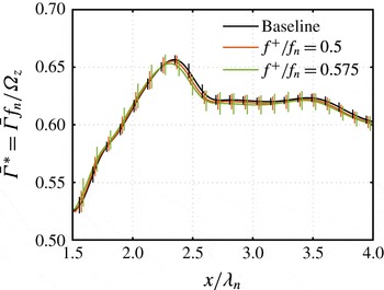
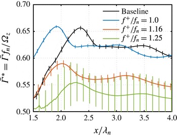
Normalized ensemble averaged vortex circulation (
 $\bar{\unicode[STIX]{x1D6E4}}^{\ast }$
) and its variation (vertical bars) for cases with
 $\unicode[STIX]{x1D703}_{0}/w=0.1$
. We normalized the average circulation,
 $\bar{\unicode[STIX]{x1D6E4}}$
, by the characteristic vorticity that is fed to each vortex in the roll-up period,
 $\unicode[STIX]{x1D6FA}_{z}/f_{n}$
, from two streams. Low-frequency forcing does not significantly change the mean strength but introduces greater variation in the strength of each vortex.

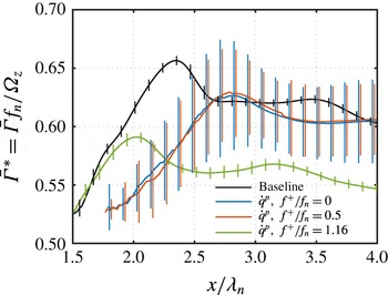
As pointed out in § 4, the thermal actuation can produce oscillatory vorticity flux over the trailing edge. This extra fluctuating vorticity generation is in turn fed to each formed vortex and leads to variation in its strength from one vortex to another. This is shown in figure 11, where the normalized circulation at each streamwise station is averaged over each formed vortex. We observed that, in both forced cases, the mean vortex strength does not significantly change from that of the baseline, but the variation in strength is larger. The variation in vortex strength can tip over the spatial balance from one vortex to another, resulting in its trajectory deviation from the centreline. The spread of the shear layer can be attributed to both the random trajectory deviation and the vortex merging process. As the strength variation in
 $f^{+}/f_{n}=0.575$
is greater than that in
 $f^{+}/f_{n}=0.500$
, the trajectory deviation and merging are indeed taking place earlier for
 $f^{+}/f_{n}=0.575$
than for
 $f^{+}/f_{n}=0.500$
.
Transverse velocity spectra at
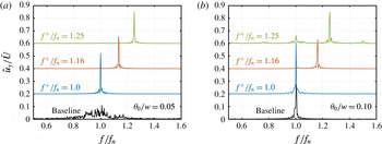
 $x/\unicode[STIX]{x1D706}_{n}=3.0$
; the shedding is observed to lock onto the forcing frequency when
 $f^{+}/f_{n}\in [1.00,1.25]$
: (a)
 $\unicode[STIX]{x1D703}_{0}/w=0.05$
; (b)
 $\unicode[STIX]{x1D703}_{0}/w=0.1$
. The spectra are shifted vertically for graphical clarity.

The forcing effects with
 $f^{+}/f_{n}=0.500$
and
 $0.575$
in the cases of initial momentum thicknesses of
 $\unicode[STIX]{x1D703}_{0}/w=0.05$
and
 $0.25$
are qualitatively similar to the case of
 $\unicode[STIX]{x1D703}_{0}/w=0.1$
discussed above. Additional discussions for these two
 $\unicode[STIX]{x1D703}_{0}/w$
cases are provided in appendix B.
5.2 Excitation of fundamental roll-up (
$f^{+}\approx f_{n}$
)

Let us discuss the forcing effects when the forcing frequency is close to
 $f_{n}$
with the use of
 $\dot{q}$
(2.7). We consider forcing frequencies of
 $f^{+}/f_{n}=1.0$
,
 $1.16$
and
 $1.25$
with
 $\unicode[STIX]{x1D703}_{0}/w=0.1$
and
 $\unicode[STIX]{x1D703}_{0}/w=0.05$
. All cases presented in this section are of the same forcing power of
 $E^{+}=0.741$
. Although we have also studied forced flow with forcing frequency up to
 $f^{+}/f_{n}=16$
, no significant change in the forced two-dimensional shear layer is observed for cases with
 $f^{+}/f_{n}\geqslant 2$
.
Figure 12 shows the transverse velocity spectra for the baseline and forced cases with
 $f^{+}/f_{n}=1.00$
,
 $1.16$
and
 $1.25$
at a streamwise station of
 $x/\unicode[STIX]{x1D706}_{n}=3$
on the centreline. As discussed in § 3, the stronger wake effect in
 $\unicode[STIX]{x1D703}_{0}/w=0.05$
baseline flow leads to a less synchronized shear layer roll-up and a spectrum with a broader distribution of energy across frequencies. With periodic heating at the frequencies considered here, we find that the forcing is able to lock the roll-up onto the forcing frequency, indicated by the prominent peak at the corresponding forcing frequency for each case for both
 $\unicode[STIX]{x1D703}_{0}/w=0.05$
and
 $0.1$
in figures 12(a) and 12(b) respectively.
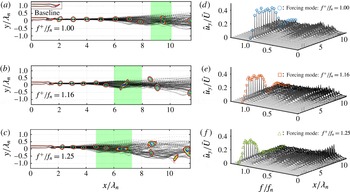
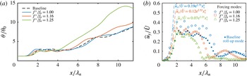
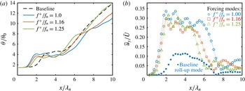
Analogously to the discussion for low-frequency forced cases, in figures 13 and 14 we show the vortex trajectories and spatial revolution of transverse velocity spectra and momentum thicknesses for the baseline and three forced cases. The thermal forcing input serves as an excitation to the fundamental instability wave and encourages the shear layer roll-up at the forcing frequency. In the cases with
 $f^{+}/f_{n}=1.0$
and
 $1.16$
, the thermal forcing results in earlier shedding than that of the baseline. This can be seen by comparing the instantaneous vorticity contours in the initial shedding region: in both cases of
 $f^{+}/f_{n}=1.0$
and
 $1.16$
, the vorticity sheet formed from
 $x/\unicode[STIX]{x1D706}_{n}=0$
starts to carry a streamwise instability wave earlier than the baseline. Earlier roll-up can also be identified from the first rapid growth of
 $\unicode[STIX]{x1D703}/\unicode[STIX]{x1D703}_{0}$
in figure 14(a).
Vortex trajectories (a–c) and modal amplitude growth (d–f) for
 $\unicode[STIX]{x1D703}_{0}/w=0.1$
cases. With
 $f^{+}$
close to
 $f_{n}$
, the forcing is able to excite the shear layer roll-up and accelerate the roll-up process.

(a) Momentum thickness growth and (b) modal amplitude growth for cases with
 $\unicode[STIX]{x1D703}_{0}/w=0.1$
and
 $f^{+}/f_{n}=1.0$
,
 $1.16$
and
 $1.25$
.

Vortex strength for cases of
 $\unicode[STIX]{x1D703}_{0}/w=0.1$
with
 $f^{+}/f_{n}=1.0$
,
 $1.16$
and
 $1.25$
. In the control cases where the roll-up frequency is locked onto the actuation frequency, the mean strength of the formed vortex is changed accordingly. With greater variation in the strength of each vortex, enhanced spreading of the shear layer is also observed.

With
 $f^{+}/f_{n}=1.0$
, synchronized shear layer roll-up due to forcing can also be observed from the uniform spacing between each vortex in the vortex train, as shown in figure 13(a). Moreover, the forcing is able to suppress the vortex deviating from the centreline. This leads to an extended isolated vortex region with forcing, suggested by the wider flat region in the range
 $1\leqslant x/\unicode[STIX]{x1D706}_{n}\leqslant 5$
in figure 14(a).
The spatial development of the frequency spectra and the modal amplitude growth are shown in figures 13(d–f) and 14(b) respectively. For the three forced cases, the amplitudes of the modes with their frequencies corresponding to the actuation frequencies start to grow immediately behind the trailing edge at
 $x/\unicode[STIX]{x1D706}_{n}=0$
, and their growth rates are well predicted by the local stability analysis, as shown in figure 14(b). When the forcing frequency departs farther from
 $f_{n}$
, the growth rate decreases, as observed for
 $x/\unicode[STIX]{x1D706}_{n}\leqslant 2$
. This can be attributed to the instability characteristics of the shear layer. When the forcing frequency is closer to
 $f_{n}$
, the frequency with the highest spatial growth rate for the perturbation, the forcing effort grows faster since the growth rate is approaching its maximum.
The frequency spectra of the three forced cases all have distinct peaks at the forcing frequency initially for
 $x/\unicode[STIX]{x1D706}_{n}\leqslant 3$
. As
 $x/\unicode[STIX]{x1D706}_{n}>3$
, lower-frequency modes start to grow and the momentum thickness increases accordingly, as shown in figure 14(a). With higher
 $f^{+}$
, the modal amplitude at the corresponding forcing frequency also decays spatially earlier in the range
 $5\leqslant x/\unicode[STIX]{x1D706}_{n}\leqslant 7$
. Earlier decay of the modal amplitude at the forcing frequency also coincides with the earlier growth of lower-frequency modes in the full spectra in figure 13(d–f). Especially for the case of
 $f^{+}/f_{n}=1.25$
, lower-frequency modes start to develop farther upstream compared with the baseline flow, resulting in a faster second growth of
 $\unicode[STIX]{x1D703}/\unicode[STIX]{x1D703}_{0}$
.
(a) Momentum thickness growth and (b) modal amplitude growth with high-frequency forcing for the
 $\unicode[STIX]{x1D703}_{0}/w=0.05$
cases. The accelerated roll-up and amplitude growth in the forcing mode are observed to be in qualitative agreement with cases of
 $\unicode[STIX]{x1D703}_{0}/w=0.1$
.

In the isolated vortex region for the forced cases, thinner
 $\unicode[STIX]{x1D703}$
is observed when using higher
 $f^{+}$
. This can be explained by the weaker vortex strength considering that the total vorticity flux is introduced from the inlet boundary at the same rate. With these compact vortices convecting at the mean shear layer velocity, the higher vortex passage frequency leads to a lower amount of vorticity being possessed by the individual vortices, which can be confirmed from figure 15. For the cases with
 $f^{+}/f_{n}=1.16$
and
 $1.25$
, the mean vortex strengths are lower than those from the baseline and
 $f^{+}/f_{n}=1.0$
cases. With weaker vortices, the reduced mixing of momentum from two streams leads to a smaller momentum thickness in the isolated vortex region. Moreover, the strength variations in the cases of
 $f^{+}/f_{n}=1.16$
and
 $1.25$
are greater than that of the baseline. This again leads to faster shear layer spreading than the baseline, similarly to the low-frequency forced cases. With
 $f^{+}/f_{n}=1.0$
, on the other hand, the smaller variation in vortex strength leads to a more stable isolated vortex region, leading to a wider streamwise extent than that of the baseline, as shown in figure 14(a).
For cases with
 $\unicode[STIX]{x1D703}_{0}/w=0.05$
, the lock-on of the shear layer roll-up frequency and the extended isolated vortex region are still observed when forcing is invoked with
 $f^{+}/f_{n}=1.00$
,
 $1.16$
and
 $1.25$
, as shown in figures 12 and 16. However, we also note that for
 $\unicode[STIX]{x1D703}_{0}/w=0.25$
cases, no significant changes can be seen in the shear layer for
 $f^{+}/f_{n}=1.00$
and
 $1.16$
, even when using a forcing amplitude of
 $E^{+}=0.724$
, four times the value considered earlier in this section.
5.3 Roll-up delay (positive-mean heating)
In this section, the forcing effects in the shear layer from using
 $\dot{q}^{p}$
(2.8) are investigated. This form of forcing,
 $\dot{q}^{p}$
, is composed of a positive DC offset added to the oscillatory
 $\dot{q}$
. The positive DC offset introduces net positive heat transfer from the actuator and raises the mean temperature of the fluid adjacent to the actuator. With the temperature-varying viscosity model discussed in § 2.2, this locally increased temperature leads to a higher viscosity.
Vortex trajectories (a–c) and modal amplitude growth (d–f) for
 $\unicode[STIX]{x1D703}_{0}/w=0.1$
cases. The merging location and its spatial variation are depicted by the green-shaded region (a–c) in each case.

(a) Momentum thickness growth and (b) modal amplitude growth for low-frequency forcing (
 $\unicode[STIX]{x1D703}_{0}/w=0.1$
).

Vortex strength for cases of
 $\unicode[STIX]{x1D703}_{0}/w=0.1$
. In the cases with roll-up delay, the vortex strength is observed to have greater variation and encourage spreading of the shear layer downstream. All cases are for
 $\unicode[STIX]{x1D703}_{0}/w=0.1$
.

We consider representative forced cases with
 $E^{+}=0.741$
. The effects of the locally increased viscosity are shown in figure 17(a–c). Comparing the cases with
 $f^{+}/f_{n}=0$
(i.e. constant heating) and
 $0.500$
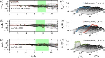
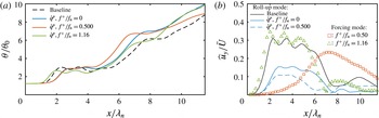
with the baseline, the shear layer roll-up is delayed due to the locally increased viscosity. The delayed shear layer roll-up leads to an elongated recirculation region behind the trailing edge and introduces a stronger wake effect. As a consequence, the roll-up is observed to be less synchronized, as depicted in figure 17(d–f) by the less prominent peak in the roll-up mode in the spectra of the DC heating and
 $f^{+}/f_{n}=0.500$
cases. The growth in the roll-up mode is also observed to reach a lower maximum amplitude than it does in the baseline flow, as shown in figure 18(b). With the stronger wake effect and the less synchronized roll-up, the vortex strength exhibits greater variation, as shown in figure 19. By the same mechanism as discussed in the previous sections, the higher variation leads to early deviations of the trajectories from the centreline, as well as early merging of the vortices. Both of these effects cause the shear layer to spread faster downstream in the cases with DC heating and
 $f^{+}/f_{n}=0.500$
. The delayed roll-up and accelerated spreading can also be observed in the growth of
 $\unicode[STIX]{x1D703}/\unicode[STIX]{x1D703}_{0}$
from figure 18(a). With the subharmonic forcing added, the
 $f^{+}/f_{n}=0.500$
case exhibits a greater growth in
 $\unicode[STIX]{x1D703}$
compared with the DC heating case. In the case with
 $f^{+}/f_{n}=1.16$
, the oscillatory component of
 $\dot{q}^{p}$
dominates over the DC component and still accelerates the shear layer roll-up. The changes in the vortex trajectories (figure 17
a–c), vortex strength (figure 19),
 $\unicode[STIX]{x1D703}/\unicode[STIX]{x1D703}_{0}$
growth (figure 18
a) and forcing mode growth (figure 18
b) show similar traits to those observed in the case using
 $\dot{q}$
with
 $f^{+}/f_{n}=1.16$
.
Effects of forcing amplitude (
 $E^{+}$
) in the DC heating and subharmonic forced cases with
 $\dot{q}^{p}$
. All cases are for
 $\unicode[STIX]{x1D703}_{0}/w=0.1$
.

In the subharmonic forced case with
 $\dot{q}^{p}$
, the accelerated merging built upon the delayed roll-up draws additional interest. Motivated by the observations, for cases of DC heating and
 $f^{+}/f_{n}=0.500$
, we further examine the effects of the forcing amplitude,
 $E^{+}$
, on the growth of
 $\unicode[STIX]{x1D703}$
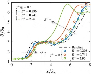
, as shown in figure 20. We observe that the shear layer roll-up location, suggested by the first growth in
 $\unicode[STIX]{x1D703}$
, is delayed farther downstream with increased
 $E^{+}$
in both DC heating and subharmonic forced cases. Meanwhile, the acceleration in the spreading (second growth of
 $\unicode[STIX]{x1D703}$
) is also enhanced by the subharmonic forcing with increasing
 $E^{+}$
.
Comparing the forcing effects of
 $\dot{q}$
and
 $\dot{q}^{p}$
, we observe that the oscillatory components from both types impose similar forcing effects on the shear layer. The positive DC component in
 $\dot{q}^{p}$
is able to delay the shear layer roll-up when it is not excited by the oscillatory component.
6 Concluding remarks
We numerically examined the effectiveness of local periodic heating in modifying a spatially developing shear layer downstream of a splitter plate. The early evolution of the baseline shear layer is characterized by three regions, namely a region where vortices roll up, a second region where vortices advect along the centreline and a third region where vortices deviate from the centreline, leading to a merging process. The periodic heating from the trailing edge introduces a thermal perturbation to the fluid adjacent to the actuator and consequently generates oscillatory vorticity flux over its surface and baroclinic torque in its vicinity. These added sources of vorticity perturb the strength of the vortices formed from the shear layer roll-up, and result in a change in the shear layer dynamics.
Three-dimensional LES of shear layers with
 $\unicode[STIX]{x1D703}_{0}/w=0.1$
for the baseline and controlled cases (
 $f^{+}/f_{n}=1.16$
). The flow visualization uses the
 $Q$
-isosurface coloured by the streamwise velocity and the isosurface of vorticity magnitude overlaid in transparent grey.

The spatial evolution of the vortex orientation. The spatial oscillation in the
 $\unicode[STIX]{x1D703}/\unicode[STIX]{x1D703}_{0}$
profile in the isolated vortex region is caused by the orientation of the elliptic vortices.

Vortex trajectories (a–c) and modal amplitude growth (d–f) for the
 $\unicode[STIX]{x1D703}_{0}/w=0.25$
cases. The merging location and its spatial variation are depicted by the green-shaded region (a–c) in each case.

Momentum thickness growth (a,b) and modal amplitude growth (c,d) with low-frequency forcing for cases with
 $\unicode[STIX]{x1D703}_{0}/w=0.25$
(a,c) and
 $\unicode[STIX]{x1D703}_{0}/w=0.05$
(b,d). In (c,d), ▫ represents the forcing mode with
 $f^{+}/f_{n}=0.500$
and ○ represents
 $f^{+}/f_{n}=0.575$
.

This thermal actuation technique is shown to be capable of serving as an excitation source for both the fundamental and subharmonic instabilities. When using the forcing frequency close to the first subharmonic of the shear layer roll-up frequency, the forcing can encourage vortices to deviate from the centreline and accelerate the merging process. When the periodic heating excites the shear layer roll-up, such forcing is able to shift the roll-up frequency to the actuation frequency and modify the mean strength of each vortex. The local momentum thickness in the isolated vortex region is also accordingly modified before further spreading takes place. Thermal actuation with positive mean is also observed to delay the shear layer roll-up. In spite of the delayed roll-up, the subharmonic oscillatory component is still able to accelerate the downstream spreading of the shear layer. We also find that the shear layer spreading rate can be characterized by the synchronized nature of the shear layer roll-up. The lower level of roll-up synchronization correlates with the greater variance in the vortex strength, less repeatable vortex trajectories and a higher spreading rate of the shear layer.
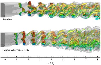
As a final note, let us briefly mention that the same control setting is observed to be effective in modifying three-dimensional free shear layers. We perform large-eddy simulations (LES) using the same set-up as in the two-dimensional simulations but extend the computational domain in the spanwise direction with an extent of
 $z/w=[-10,10]$
with spanwise periodicity. Figure 21 shows the instantaneous flow field, visualized using the isosurface of the
 $Q$
-criterion and the vorticity magnitude, for the baseline and a controlled case of
 $\unicode[STIX]{x1D703}_{0}/w=0.1$
. For the controlled case, the excitation of shear layer roll-up instability is still effective in modifying the three-dimensional shear layer with
 $f^{+}/f_{n}=1.16$
. Moreover, enhanced shear layer spreading can also be observed in the flow visualization, as indicated by the wide transverse extent of the vortical structure in the controlled case compared with the baseline flow. While the use of the present control approach requires further investigation in three-dimensional turbulent flow, the result shown exhibits promising capabilities of the present actuation technique. In fact, this type of actuation has been shown to be effective in suppressing turbulent separated flow at a chord-based Reynolds number of 23 000 over a canonical airfoil in another study by the current authors (see Yeh, Munday & Taira Reference Yeh, Munday and Taira2017), showing the potential of thermal-based flow actuation in aerodynamic flow control applications.
We have demonstrated that the nonlinear dynamics of a spatially developing shear layer can be modified by local oscillatory heat flux as a control input. This thermal-energy-deposition-based actuation is able to trigger shear layer instability without relying on mass or momentum injections, and can be considered as a potential candidate for a flow control actuation mechanism for a range of applications, especially those that do not permit internal installation space for actuators or sizable weight additions. We believe that this study provides a foundation for flow control using modern thermal-energy-based actuators.
Acknowledgements
The authors acknowledge the US Army Research Office for supporting this project (Award no. W911NF-14-1-0224). The computations were supported by the High Performance Computing Modernization Program at the Department of Defense and the Research Computing Center at Florida State University.
Appendix A. Spatial oscillation in momentum thickness over the isolated vortex region
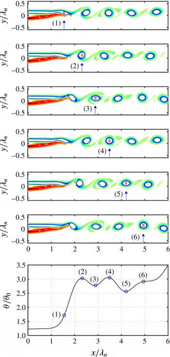
This spatial variation in the momentum thickness profile in the isolated vortex region is due to the changing orientation of the elliptic vortices. This spatial evolution in the vortex orientation is illustrated in figure 22 with six snapshots of instantaneous vorticity field (top) and the momentum thickness profile (bottom) with the spatial oscillation. It should be noted that the flow fields are visualized in equal aspect ratio in both the streamwise and transverse directions. We clearly observe that, at stations (3) and (5), the vortex is horizontally stretched, and the
 $\unicode[STIX]{x1D703}/\unicode[STIX]{x1D703}_{0}$
profile exhibits a local minimum. On the other hand, at stations (2), (4) and (6), the vortex appears to be circular in shape and results in a thicker
 $\unicode[STIX]{x1D703}/\unicode[STIX]{x1D703}_{0}$
.
Appendix B. Subharmonic forced cases for
$\unicode[STIX]{x1D703}_{0}/w=0.05$
and
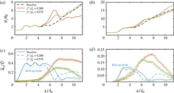
$0.25$


We find noteworthy effects with subharmonic forcing using
 $\hat{q}$
in the case with
 $\unicode[STIX]{x1D703}_{0}/w=0.25$
, as shown in figure 23. Even though the vortex starts to deviate from the centreline earlier in both of the forced cases compared with the baseline, the vortex merging process takes place in a more repetitive (locked) manner when forcing is introduced at the first subharmonic of the roll-up frequency. The ordered and repetitive trajectories for
 $f^{+}/f_{n}=0.500$
leave a white region absent of any trajectories around
 $x/\unicode[STIX]{x1D706}_{n}\approx 6.5$
, where no vortices have travelled through. The use of a subharmonic frequency allows for vortex merging by successive pairs along the vortex train. Moreover, after merging, the vortex trajectories show significantly more reduction in their variations in the subharmonic forced case than in the
 $f^{+}/f_{n}=0.575$
case. The growth rates of the modal amplitudes are shown in figure 24(c,d), where the modal amplitudes at both forcing frequencies are amplified downstream. The modal amplitude at the forcing frequency in the
 $f^{+}/f_{n}=0.500$
case maintains its high level while marching downstream, and suppresses other lower frequency modes from growing, as highlighted by the clean spectra in the green circled region compared with the baseline and
 $f^{+}/f_{n}=0.575$
cases in figure 23(d–f), due to reduced spillage of the modal energy at the forcing frequency. Since the growth of other low-frequency modes causes the shear layer to keep spreading downstream, the slower growth in
 $\unicode[STIX]{x1D703}$
, as shown in figure 24(a,b) for both
 $\unicode[STIX]{x1D703}_{0}$
cases, can also be attributed to the absence of these lower-frequency modes.