
1. Introduction
Irregularities in bottom topography play a pivotal role in the dynamics of the ocean's circulation (Marshall Reference Marshall1995; Gille, Metzger & Tokmakian Reference Gille, Metzger and Tokmakian2004). It has been shown that oceanic mesoscale eddies and ubiquitous multiple alternating jets form and exhibit significant variability localised over topographic features (Thompson & Richards Reference Thompson and Richards2011; Boland et al. Reference Boland, Thompson, Shuckburgh and Haynes2012; Chen, Kamenkovich & Berloff Reference Chen, Kamenkovich and Berloff2015; Stern, Nadeau & Holland Reference Stern, Nadeau and Holland2015; Khatri & Berloff Reference Khatri and Berloff2018; Lazar, Zhang & Thompson Reference Lazar, Zhang and Thompson2018; Khatri & Berloff Reference Khatri and Berloff2019). This variation in oceanic flows and flow–topographic interactions affect many processes such as the eddy-induced transport, eddy energetics and ocean ventilation (Thompson Reference Thompson2010; Abernathey & Cessi Reference Abernathey and Cessi2014; Barthel et al. Reference Barthel, McC. Hogg, Waterman and Keating2017; Tamsitt Reference Tamsitt2017; Youngs et al. Reference Youngs, Thompson, Lazar and Richards2017; Klocker Reference Klocker2018).
A primary impact of changes in the structure of the ocean bottom is the modification of baroclinic growth rates in regions upstream and downstream of topography (Thompson & Sallée Reference Thompson and Sallée2012; Abernathey & Cessi Reference Abernathey and Cessi2014; Thompson & Naveira Garabato Reference Thompson and Naveira Garabato2014; Chapman et al. Reference Chapman, McC. Hogg, Kiss and Rintoul2015; Youngs et al. Reference Youngs, Thompson, Lazar and Richards2017). Consequently, eddies tend to be very energetic downstream of topography, resulting in regions with large eddy-induced meridional transport (Tamsitt Reference Tamsitt2017). In view of the complexity of flow–topographic interactions present, many simplifications are made when addressing oceanic flow stability in the literature. The simplest approach to investigating flow instability is assuming a flat ocean bottom, which has been the focus of various works (Orlanski & Cox Reference Orlanski and Cox1972; Tang Reference Tang1975; Killworth Reference Killworth1980; Niino & Misawa Reference Niino and Misawa1984), while a barotropic dynamics has also been assumed in many papers to explore stability over topographic features (Benilov Reference Benilov2000a,Reference Benilovb; Vanneste Reference Vanneste2003; Benilov, Nycander & Dritschel Reference Benilov, Nycander and Dritschel2004).
Despite these simplistic frameworks being beneficial to work with from a mathematical perspective, it is still important to consider the topographic effects on baroclinic instability as it is a crucial process impacting the large-scale ocean circulation. A number of studies have engaged in the linear stability analysis and shown that topographic slopes greatly affect the baroclinic-instability growth rates (Hart Reference Hart1975a,Reference Hartb; Sutyrin Reference Sutyrin2007; Chen & Kamenkovich Reference Chen and Kamenkovich2013; LaCasce et al. Reference LaCasce, Escartin, Chassignet and Xu2019). More specifically, Chen & Kamenkovich (Reference Chen and Kamenkovich2013) concluded that zonal flows are strongly destabilised by zonal slopes (i.e. flow perpendicular to isobaths) due to the potential vorticity (PV) gradient obtaining an additional zonal component. In this instance, even small-scale topography can result in destabilisation, with the magnitude of the largest growth rates increasing with elevated bottom relief. On the other hand, meridional slopes (i.e. surface shear parallel to isobaths) are shown to either stabilise or destabilise zonal flows through altering the PV gradient in the bottom fluid layer. Such suppression of baroclinic instability is in accord with the findings of LaCasce et al. (Reference LaCasce, Escartin, Chassignet and Xu2019), who instead consider a zonal jet. In particular, suppression over large topographic slopes is stronger (weaker) when the flow is perpendicular (parallel) to the topography propagation.
The effect of sinusoidal bottom topography on baroclinic instability in a two-layer quasigeostrophic (QG) model has been studied with an asymptotic expansion method (Benilov Reference Benilov2001). These results, which are only applicable to small-scale topography, i.e. topographic height and horizontal spatial scale taken to be 200 m and 5 km, respectively, suggest that bottom irregularities of this nature suppress baroclinic instability when the isobaths are parallel to the vertical velocity shear, and have no influence when the isobaths are perpendicular. Alterations of layer depths are also considered, which suggest topography has a weak (strong) effect on flows localised in thin (thick) upper layers (Benilov Reference Benilov2001).
The more recent study Radko (Reference Radko2020), which considers the influence of submesoscale sinusoidal topography on baroclinic instability in both a multi-layer QG and shallow-water models, makes use of a method of multiple scales expansion by exploiting short topographic wavelengths of 1–10 km. The results are verified with doubly periodic numerical solutions (Radko Reference Radko2020), and similar to Benilov (Reference Benilov2001), indicate a suppression in baroclinic instability by submesoscale topography. Furthermore, linear stability solutions in LaCasce et al. (Reference LaCasce, Escartin, Chassignet and Xu2019) support submesoscale stabilisation by demonstrating that a sinusoidal ridge with an amplitude of 10 m and wavelength of 1 km is enough to suppress baroclinic instability.
The primary focus of the present study is to examine how a variable ocean bottom affects the most unstable linear modes in a baroclinic QG model. For this purpose, we consider sinusoidal topographic variation in either the zonal or meridional direction, and carry out the corresponding linear stability analyses. In particular, we are interested in the effects of large-scale topography on baroclinic instability. We do not deal with small-scale topographic features as higher baroclinic modes may be important in the interaction between baroclinic modes and topography, and to obtain this information requires are greater computational expenditure. Nonetheless, we compare our findings with the small-scale sinusoidal topography studies discussed since large-scale topography considerations are normally restricted to topographic slopes. Moreover, this will identify how results obtained using different methods and assumptions resemble and differ to our linear stability results.
The presence of variable topography introduces a nonlinear term, i.e. product of topography and perturbation streamfunction, in linearised equations and it is required to solve a generalised eigenvalue problem for linear stability analysis. For example, LaCasce et al. (Reference LaCasce, Escartin, Chassignet and Xu2019) used Chebyshev grid discretisation in the meridional direction. We could investigate the influence bottom topography has on baroclinic instability by discretising the linearised governing equations with respect to physical space in the direction of changes in topographic height. Such a method yields a complex eigenvalue problem with coupled eigenmodes; e.g. Berloff & Kamenkovich (Reference Berloff and Kamenkovich2013) and Khatri & Berloff (Reference Khatri and Berloff2019) used finite-difference discretisation to study the stability of multiple jets. However, this technique is computationally taxing, as it is relatively sensitive to the numerical grid resolution, which can be rather fine for obtaining numerically convergent results.
Instead, we use spectral discretisation in terms of Fourier modes applied in both spatial directions and construct an eigenvalue matrix in terms of Fourier eigenmodes. Since the topography has its own length scales, the eigenmodes in the direction of varying topography become coupled. For example, in the case of a topography changing in the meridional direction only, our method results in a complex eigenproblem having coupled Fourier modes along the meridional wavenumber for each zonal wavenumber. An advantage of this approach is that it can be used for any periodic topography, and the limiting assumptions of the QG approximation are the only restrictions on the topography considered. Furthermore, it is computationally efficient because the linear stability problem can be solved with a limited number of wavenumbers provided the considered spectral resolution is adequate to resolve baroclinic instability.
In this study, we adopt a QG approximation as working with other circulation models is computationally challenging, and it is wise to explore the ground before engaging them; especially, since Radko (Reference Radko2020) suggests similarity between the shallow-water and QG responses. On the other hand, we expect significant differences to arise in more realistic model configurations, hence extending into the primitive equations is desirable in the future. Regardless, these differences will only be significant in the nonlinear regime, and so the use of QG is sufficient for performing a linear stability analysis. Moreover, shallow-water and primitive equations are more appropriate in the case of small-scale topography since the QG approximation can break down as a consequence of the topographic beta term increasing a lot in comparison with the planetary beta term.
To summarise the layout of this work, in § 2 we introduce the two-layer QG equations and derive a non-dimensional system. From this, we linearise the non-dimensional model with sinusoidal topography, and formulate the corresponding eigenvalue problems. We discuss our linear stability solutions in § 3, giving justifications for the parameter values chosen. A comparison between the flat-bottom and sinusoidal topography cases is made. In particular, we look at fluctuations in the number and distribution of unstable modes, as well as in their growth rates, in response to variations in topographic width and height. Perturbation eigenmodes corresponding to the maximum unstable growth rate are presented and the linear stability analysis is extended to a thin-upper-layer case. Finally, § 4 acts as a conclusion to the paper, summarising the work presented and suggesting some additions that can be made in the future. For completeness, we include the technical details for solving the derived eigenproblems in appendix A.
2. Two-layer QG approximation
In this investigation, we consider a two-layer rigid-lid model on an  $(\hat {x}, \hat {y})$-Cartesian
 $\hat {\beta }$-plane in the presence of variable bottom irregularities (a schematic is shown in figure 1), which we denote by
 $\hat {\eta }_b(\hat {x}, \hat {y})$. For our purposes, we assume a zonally uniform background flow,
 $\hat {U}$, in the top fluid layer, with the bottom layer simply at rest. The need for this vertical velocity shear is to induce baroclinic instability in the system. In this work, we adopt the QG approximation (figure 1), and write the fully nonlinear model equations as (Vallis Reference Vallis2017)
 \begin{equation} \frac{\partial \hat{\varPi}_j}{\partial \hat{t}} + \mathbb{J}(\hat{\psi}_j - \delta_{1j}\hat{U}\hat{y}, \hat{\varPi}_j) = \hat{\nu}\hat{\nabla}^{4}\hat{\psi}_j - \delta_{2j}\hat{\gamma}\hat{\nabla}^{2}\hat{\psi}_j, \end{equation}
where  $j = 1, 2$ refer to the reference layer (the top layer corresponds to
 $j = 1$ and the bottom layer corresponds to
 $j = 2$). The layer-wise streamfunction is denoted by
 $\hat {\psi }_j$ and
 $\delta _{ij}$ identifies the Kronecker delta. The parameters
 $\hat {\nu }$ and
 $\hat {\gamma }$ are representative of eddy viscosity and bottom friction, respectively. The Jacobian operator is defined as
 \begin{equation} \mathbb{J}(A, B) = \frac{\partial A}{\partial \hat{x}}\frac{\partial B}{\partial \hat{y}} - \frac{\partial A}{\partial \hat{y}}\frac{\partial B}{\partial \hat{x}}, \end{equation}
and the layer-wise PV is given by
 \begin{equation} \hat{\varPi}_j = \underbrace{\hat{\nabla}^{2}\hat{\psi}_j + \hat{S}_j(\hat{\psi}_{3 - j} - \hat{\psi}_{j})}_{\text{PV anomaly},\ \hat{\rm \pi}_j} + \bigg[\hat{\beta} + \hat{S}_j\hat{U} (\delta_{1j} - \delta_{1, 3 - j})\bigg]\hat{y} + \frac{\delta_{2j}\hat{f}_0\hat{\eta}_b}{\hat{H}_j}. \end{equation}
Illustration of the model domain. An eastward background velocity is imposed in the surface layer, with the bottom layer at rest. Bottom topography, mean layer depths and density anomalies are denoted by  $\hat {\eta }_b$,
 $\hat {H}_j$ and
 $\hat {\rho }_j$, respectively (
 $j = 1, 2$ is the layer index). The positive
 $\hat {x}$-axis is directed to the right and the positive
 $\hat {y}$-axis points into the figure.

In our definition for PV, we have the layer-wise stratification parameter,  $\hat {S}_j = \hat {f}_0^{2}/\hat {g}^{\prime } \hat {H}_j$, with reduced gravity defined in terms of layer-wise density anomalies and gravitational acceleration, i.e.
 $\hat {g}^{\prime } = \hat {g}{\rm \Delta} \hat {\rho }/\hat {\rho }_1$,
 ${\rm \Delta} \hat {\rho } = \hat {\rho }_2 - \hat {\rho }_1$ and
 $\hat {H}_j$ referring to the mean layer depths. Furthermore,
 $\hat {\beta }$ is the meridional gradient of the Coriolis parameter,
 $\hat {f} = \hat {f}_0 + \hat {\beta } \hat {y}$, where
 $\hat {f}_0$ is the angular velocity due to the Earth's rotation at some reference latitude. For clarity, dimensional quantities are notated with hats. We proceed by neglecting terms due to eddy viscosity and bottom friction as they do not have any major effects on the solutions obtained from a linear stability analysis.
2.1. Non-dimensionalisation
To highlight the key parameter values in our stability analysis, it is convenient to non-dimensionalise (2.1). In our case, we introduce the horizontal length scale  ${\hat {L}_H = \hat {L}/2{\rm \pi}}$, where the zonal and meridional length of the domain is
 $\hat {L} = \hat {L}_X = \hat {L}_Y$, and the presence of
 $2{\rm \pi}$ acts to normalise angular frequencies and wavenumbers later on. More specifically, we choose
 $\hat {L} = \sqrt {\hat {g}\hat {H}}/\hat {f}_0,$ where we have
 $\hat {H} = \sum _{i=1}^{2}\hat {H}_i$ defining the total mean layer depth. Moreover, we choose
 $\hat {L}_V = \hat {H}$,
 $\hat {T} = 1/\hat {f}_0$ and
 $\hat {V} = \hat {f}_0\hat {L}/2{\rm \pi}$ to be our vertical length scale, time scale and velocity scale, respectively. Thus, we obtain the non-dimensional transformation
 \begin{equation} (\hat{x}, \hat{y}) = \frac{\hat{L}}{2{\rm \pi}} (x, y),\quad \hat{t} = \frac{t}{\hat{f}_0},\quad \hat{U} = \frac{\hat{f}_0\hat{L}}{2{\rm \pi}}U,\quad \hat{\psi}_j = \frac{\hat{f}_0\hat{L}^{2}}{4{\rm \pi}^{2}}\psi_j,\quad \hat{\eta}_b = \hat{H}\eta_b, \end{equation}
where the dimensionless quantities we have introduced are notated without hats. Therefore, applying (2.4a–e) to (2.1), we arrive at the following non-dimensional system:
 \begin{equation} \frac{\partial \varPi_j}{\partial t} + \mathbb{J}(\psi_j - \delta_{1j}Uy, \varPi_j) = 0, \end{equation}
where we define the non-dimensional PV by
 \begin{equation} \varPi_j = \nabla^{2}\psi_j + S_j(\psi_{3-j} - \psi_j) + \Bigg[\beta + S_jU(\delta_{1j} - \delta_{1, 3 - j})\Bigg]y + \frac{\delta_{2j}\hat{H}\eta_b}{\hat{H}_j}, \end{equation}
with  $\beta = \hat {L}\hat {\beta }/2{\rm \pi} \hat {f}_0$ and
 $S_j = \hat {L}^{2}\hat {S}_j/4{\rm \pi} ^{2}$.
2.2. Linearised model with sinusoidal topography
We now turn our attention to the linear stability problem for this set-up. Since nonlinear terms are only due to the Jacobian, we can expand this operator and identify nonlinearities in  $\hat {\psi }_j$. Thus, by means of linearisation, we obtain the linear system of equations
 \begin{align} \left(\frac{\partial}{\partial t} + \delta_{1j}U\frac{\partial}{\partial x}\right){\rm \pi}_j + \frac{\partial \psi_j}{\partial x}\left[\beta + S_jU(\delta_{1j} - \delta_{1, 3 - j}) + \frac{\delta_{2j}\hat{H}}{\hat{H}_j}\frac{\partial \eta_b}{\partial y}\right] - \frac{\delta_{2j}\hat{H}}{\hat{H}_j}\frac{\partial \psi_j}{\partial y}\frac{\partial \eta_b}{\partial x} = 0, \end{align}
with non-dimensional PV anomaly given by
 \begin{equation} {\rm \pi}_j = \nabla^{2}\psi_j + S_j(\psi_{3-j} - \psi_j). \end{equation}
To formulate the stability problem in the presence of sinusoidal bottom topography, we assume for simplicity that the bottom irregularities in question are either zonal or meridional, but never both. That is, we consider both sinusoidal zonally oriented multiple ridges (ZR),
 \begin{equation} \hat{\eta}_b = \hat{\mathcal{A}}\sin (\hat{\alpha} \hat{y}), \end{equation}
and sinusoidal meridionally oriented multiple ridges (MR),
 \begin{equation} \hat{\eta}_b = \hat{\mathcal{A}}\sin (\hat{\alpha} \hat{x}), \end{equation}
where  $\hat {\mathcal {A}} = \hat {H}\mathcal {A}$ and
 $\hat {\alpha } = 2{\rm \pi} \alpha /\hat {L}$ are amplitude and wavenumber parameters, respectively, for bottom topography (figure 2). More concretely, the non-dimensional variable
 $\alpha$ represents the number of topographic ridges under consideration (increasing this value amounts to decreasing ridge width). Note that the non-dimensional forms of the bottom topographies in this work are
 \begin{equation} \eta_b = \begin{cases} \mathcal{A}\sin(\alpha y) & \text{(ZR)}, \\ \mathcal{A}\sin(\alpha x) & \text{(MR)}. \end{cases} \end{equation}
Example of topographic features considered in this study: (a) zonally oriented multiple ridges (ZR); (b) meridionally oriented multiple ridges (MR).

We consider sinusoidal topography variations with a single wavelength, which is rather simple in comparison with the real ocean bathymetry. Nevertheless, the method described has the benefit of being applicable to any periodic topographic features.
With (2.9a) and (2.9b) in mind, expressing (2.7) in terms of perturbation streamfunctions and PV fields yields
 \begin{gather} \left(\frac{\partial}{\partial t} + \delta_{1j}U\frac{\partial}{\partial x}\right){\rm \pi}_j + \frac{\partial \psi_j}{\partial x}\left[\beta + S_jU(\delta_{1j} - \delta_{1, 3 - j}) + \frac{\delta_{2j}\hat{H}\mathcal{A}\alpha\cos(\alpha y)}{\hat{H}_j}\right] = 0, \end{gather}
 \begin{gather}\left(\frac{\partial}{\partial t} + \delta_{1j}U\frac{\partial}{\partial x}\right){\rm \pi}_j + \frac{\partial \psi_j}{\partial x}[\beta + S_jU(\delta_{1j} - \delta_{1, 3 - j})] - \frac{\delta_{2j}\hat{H}\mathcal{A}\alpha \cos(\alpha x)}{\hat{H}_j}\frac{\partial \psi_j}{\partial y} = 0, \end{gather}
for ZR and MR, respectively (figure 2).
It should be noted that, although our analysis concerns with a uniform zonal flow, topography generally has a significant impact of the horizontal orientation of the flow. For example, a purely zonal flow is less likely to occur over a zonally varying topography as the flow tends to move meridionally over topographic features in order to conserve PV (e.g. see Thompson Reference Thompson2010; Boland et al. Reference Boland, Thompson, Shuckburgh and Haynes2012). However, for simplicity, we restrict the analysis in this work to zonal background flows only. For studies with non-zonal background flows, readers can refer Smith (Reference Smith2007).
2.3. Formulating the eigenvalue problem
For the purpose of this study, we consider Fourier solutions of the form
 \begin{equation} \psi_j(x, y, t) = \sum_{k, \ell}\phi_j(k, \ell)\exp({\textrm{i}(kx +\ell y - \omega t)}), \end{equation}
where  $\phi _j = \phi _j(k, \ell )$ is the non-dimensional amplitude of the perturbation streamfunction,
 $(k, \ell )$ is the non-dimensional horizontal wavevector and
 $\omega$ is the non-dimensional wave frequency. Therefore, by making use of (2.12), the PV anomaly can be expressed as
 \begin{equation} {\rm \pi}_j = \underbrace{\big[S_j\phi_{3 - j} - (k^{2} + \ell^{2} + S_j)\phi_j\big]}_{{\tilde{\rm \pi}}_j} \exp({\textrm{i}(kx + \ell y - \omega t)}), \end{equation}
and so it follows that (2.11a) and (2.11b) become
 \begin{align} & \left\{(\omega - \delta_{1j}kU){\tilde{\rm \pi}}_j - k\phi_j\left[\beta + S_j U(\delta_{1j} - \delta_{1, 3 - j}) + \frac{\delta_{2j}\hat{H}\mathcal{A}\alpha\cos(\alpha y)}{\hat{H}_j} \right]\right\} \nonumber\\ &\quad \times \exp({\textrm{i}(kx + \ell y - \omega t)}) = 0, \end{align}
 \begin{align} & \left\{(\omega - \delta_{1j}kU){\tilde{\rm \pi}}_j - k\phi_j\big[\beta + S_j U(\delta_{1j} - \delta_{1, 3 - j})\big] + \frac{\delta_{2j}\hat{H}\mathcal{A}\alpha\ell\cos(\alpha x)\phi_j}{\hat{H}_j} \right\} \nonumber\\ &\quad \times\exp({\textrm{i}(kx + \ell y - \omega t)}) = 0. \end{align}
Additionally, we can simplify (2.14a) and (2.14b) further by expressing the cosine functions in exponential form. In the case of (2.14a), this yields
 \begin{align} & \{(\omega - \delta_{1j}kU){\tilde{\rm \pi}}_j - k\phi_j[\beta + S_j U(\delta_{1j} - \delta_{1, 3 - j})\}\exp({\textrm{i}(kx + \ell y - \omega t)}) \nonumber\\ &\quad -\frac{\delta_{2j}\hat{H}\mathcal{A}\alpha k\phi_j}{2\hat{H}_j} \{\exp({\textrm{i}[kx + (\ell + \alpha)y - \omega t]}) + \exp({\textrm{i}[kx + (\ell - \alpha)y - \omega t]})\} = 0. \end{align}
In order for each term in (2.15) to have a common exponential contribution, we introduce the transformation  $\ell + \alpha \rightarrow \ell$ in the first exponential term on the second line, and
 $\ell - \alpha \rightarrow \ell$ in the second exponential term on the second line. Thus, following a similar procedure for both (2.14a) and (2.14b) (we make the transformation
 $k \pm \alpha \rightarrow k$), it is possible to eliminate exponential terms to obtain the following eigenproblems:
 \begin{align} & k[\beta + S_jU(\delta_{1j} - \delta_{1, 3 - j}) - \delta_{1j}U(k^{2} +\ell^{2} + S_j)]\phi_j + \delta_{1j}kUS_j\phi_{3 - j} \nonumber\\ &\quad + \frac{\delta_{2j}\hat{H}\mathcal{A}\alpha k}{2\hat{H}_j}[\phi_j(k, \ell - \alpha) + \phi_j(k, \ell + \alpha)] = \omega[S_j\phi_{3 - j} - (k^{2} + \ell^{2} + S_j)\phi_j], \end{align}
 \begin{align} & k[\beta + S_jU(\delta_{1j} - \delta_{1, 3 - j}) - \delta_{1j}U(k^{2} + \ell^{2} + S_j)]\phi_j + \delta_{1j}kUS_j\phi_{3 - j} \nonumber\\ &\quad -\frac{\delta_{2j}\hat{H}\mathcal{A}\alpha\ell}{2\hat{H}_j} [\phi_j(k - \alpha, \ell) + \phi_j(k + \alpha, \ell)] = \omega[S_j\phi_{3 - j} - (k^{2} + \ell^{2} + S_j)\phi_j], \end{align}
for both ZR and MR, respectively (figure 2). The approach is inspired from the work Lorenz (Reference Lorenz1972) who used the same technique to study the stability of Rossby waves on a steady zonal background flow.
We can see that the presence of sinusoidal topography leads to a phase shift resulting in the coupling of individual eigenmodes. Consequently, the linear stability problem becomes relatively expensive to solve numerically. Even considering ZR and MR separately, we are required to solve matrices of size  $2N\times 2N$, where
 $N$ is the number of wavenumbers we consider in each horizontal direction. Moreover, in the instance topography is a function of both
 $x$ and
 $y$, the resulting matrices are
 $4N^{2}\times 4N^{2}$, and so the computational taxation is far greater with this added dimension. The study of Shevchenko et al. (Reference Shevchenko, Berloff, Guerrero-López and Roman2016) deals with extremely large linear stability problems and offers methodology to solve them on a supercomputer, however, this is beyond the computational capabilities of the present work. Hence, we deal with zonal and meridional topographies separately. Regardless, it is possible to extend the mathematics in this paper to sinusoidal topography experiencing variation in both directions, or other complicated periodic topographies of interest.
For  $\omega = \omega _r + \textrm {i}\omega _i$, we obtain stable solutions, if
 $\omega _i \leq 0$, and unstable solutions, if
 $\omega _i > 0$. Since we assume coupled Fourier modes to perform the stability analysis, the problem we are required to solve becomes reasonably simple, and we expect that such a spectral method will outperform finite differences since our solutions do not have discontinuities or sharp gradients.
3. Results
3.1. Parameter justifications
To proceed, we must decide on how to truncate our Fourier series solutions. Since they sum to infinity, truncation discards information about the higher Fourier modes. We aim to consider as many wavenumbers as needed for numerical convergence of the spectral coefficients, within the range of the most unstable modes due to baroclinic instability.
Parameter values chosen in this study are shown in table 1. For the sake of simplicity, we reduce the number of parameters in our problem by assuming that layer depths are equal, i.e.  $\hat {H}_1 = \hat {H}_2 = \hat {H}_*$, such that total depth becomes
 $\hat {H} = 2\hat {H}_*$, or equivalently, the stratification parameters in each fluid layer satisfy
 $S_1 = S_2 = S_*$. Under this postulation, the coefficients of the topographic contribution in (2.16a) and (2.16b) become
 $\mathcal {A}\alpha k$ and
 $-\mathcal {A}\alpha \ell$, respectively. The stratification parameter is chosen such that the baroclinic Rossby radius,
 $\hat {\lambda } = (2\hat {S}_*)^{-1/2}$, is 25 km, which is reflective of the mid-latitude ocean (Chelton et al. Reference Chelton, DeSzoeke, Schlax, El Naggar and Siwertz1998). From table 1, it is clear that the length and width of the horizontal domain in terms of this baroclinic Rossby radius are
 $109\hat {\lambda }$. Throughout this work, we take the values of
 $\hat {f}_0$ and
 $\hat {\beta }$ to correspond with a latitude of
 $30^{\circ }$ in the northern hemisphere (the values can be found in table 1).
Main parameter values chosen for the linear stability analysis presented in the study, assuming equal layer depths. Alternative parameter values used are mentioned in the main text.

Since we are making use of the QG approximation, it is easy to show that the non-dimensional velocity in the surface layer must satisfy  $U \ll 1$ in order for the Rossby number to be very small. Furthermore, it is well known that the PV gradient in the two layers must have opposite sign for instability to occur (Pedlosky Reference Pedlosky1964); from which the critical velocity in the flat-bottom case can be found to be
 $U_c = 7.930 \times 10^{-4}$. Hence, we choose
 $U = 1.586\times 10^{-3}$ to force the system to be baroclinically unstable (the dimensional equivalent is given in table 1).
The QG approximation additionally requires small topographic amplitudes relative to the deep layer thickness,  $\hat {H}_2$, as well as gentle topographic gradients. However, in this work, we also consider large topography. In particular, the most extreme case investigated assumes
 $\alpha = 40$ and
 $\mathcal {A} = 0.2$, resulting in
 $\mathcal {A}\alpha = 8$, which is approximately 60 times greater than
 $\beta = 0.1193$. This implies the topography contribution in (2.11b) dominates the
 $\beta$ contribution. Therefore, we have to question whether our asymptotic balance when assuming the QG approximation still holds for this scale of topography on the
 $\beta$-plane. This is definitely suggestive of pushing the QG limit. Nonetheless, for the sake of a theoretical investigation, we consider such scales to analyse unstable modes for a broad range of wavenumbers. In fact, some studies have demonstrated that the QG approximation does a decent job at describing geophysical systems outside the strict limitations of QG (Williams, Read & Haine Reference Williams, Read and Haine2010).
In order to check the sensitivity of results obtained with respect to  $N$, we compared solutions obtained with
 $N = 128$, 256 and 512 wavenumbers. There were some differences between the solutions with
 $N = 128$ and
 $N = 256$, but the differences between the results with
 $N = 256$ and
 $N = 512$ were insignificant. Consequently,
 $N = 256$ is sufficient for solving baroclinic instability, and so we adopted this choice in our analysis. Also, with
 $N = 256$, the smallest resolvable wavelength is
 $2\hat {L}/N \approx 20$ km and this is sufficient to resolve baroclinic instability in our analysis.
In the case of this study, we consider large-scale topography, i.e. topographic length scales either similar to or much greater than the baroclinic Rossby deformation scale, which is the fundamental scale for the flow instabilities (see table 1). However, the studies by Benilov (Reference Benilov2001) and Radko (Reference Radko2020) deal with topography length scales smaller than the baroclinic Rossby deformation scale. Regardless, we still compare our findings with these works to identify any similarities and differences. It is worth noting we could exploit the adopted scale ratio by means of an asymptotic expansion in this parameter (this would be the reciprocal of the small parameter in Benilov (Reference Benilov2000a), i.e. the non-dimensional equivalent of  $1/\hat {L}_{Top}$ would be our small parameter). Such analysis would act well to verify the results of the present study. Regardless, we do not present this here as we do not want to lose focus of the present study by making such an excursion, despite the potential merit in such an approach.
3.2. Linear stability analysis
We solve the coupled eigenvalue problem (see (2.16a) and (2.16b)) for both ZR and MR. In the ZR (MR) case, the coupled eigenvalue problem was solved for each zonal (meridional) wavenumber separately to obtain the frequency solutions and corresponding eigenmodes. We discuss the results for a range of parameter values in the following subsections. Note that we explored for many values of topographic amplitude (from the range in table 1). However, we include results for only a selection of amplitude values considered, as there was a consistency in all the solutions obtained. However, for completeness, we include some additional results in the supplementary material attached to this paper.
3.2.1. A flat ocean bottom
First, we look at the unstable modes over a flat bottom, for which the analytical solution is well known, and later compare these results with our findings in the presence of topography. For the flat-bottom model, we solved (2.16a) with  $A = 0$, for every set of zonal and meridional wavenumbers
 $(k, l)$ separately. The distribution of unstable modes (as seen in figure 3) is such that the fastest growing mode appears at
 $l =0$ and
 $k = 13$, with dimensionless maximum growth rate
 $\omega _i = 4.632\times 10^{-3}$ (or
 $3.368 \times 10^{-7}$ s
 $^{-1}$ in dimensional form). Hence, over a flat bottom, the fastest growing mode is meridionally oriented. The magnitudes of the wavenumbers corresponding to maximum growth are tied to particular parameters of interest, namely the baroclinic Rossby deformation radius, the values of background velocity and the Coriolis gradient (for details, see Berloff, Kamenkovich & Pedlosky Reference Berloff, Kamenkovich and Pedlosky2009). In this paper, we assess the impacts of variable topography on both the baroclinic growth rates and structure of the fastest growing modes, and further compare with figure 3.
Non-dimensional growth rates  $\omega _i > 0$ over flat topography (see table 1 for parameter values): (a)
 $(\omega _i, \ell )$-plot, with meridional phase speeds
 $c^{(y)} = \omega _r/\ell$ shown in the colour bar (speeds decrease with increasing
 $\ell$); (b)
 $(\omega _i, k)$-plot, with zonal phase speeds
 $c^{(x)} =\omega _r/k$ shown in the colour bar (speeds increase with increasing
 $k$). Modes are symmetric about
 $k$ (or
 $\ell$)
 $= 0$; thus, growth rates for only positive wavenumbers are presented.

3.2.2. Zonally oriented multiple ridges
We start by analysing the frequency solutions in the presence of ZR (see figure 2a), which we obtained by solving (2.16a), in  $(\omega _i, k)$-parameter space. This particular space is chosen since meridional wavenumbers are coupled in the presence of ZR, and so we solve the eigenproblem for all values of
 $l$, while keeping
 $k$ fixed. Therefore, the frequency solutions can only be analysed for each zonal wavenumber. For more details of this procedure, refer to appendix A.
In figure 4, the growth rates of unstable modes are plotted against zonal wavenumber for a non-dimensional topographic amplitude of 0.1. The figure presents several plots, each assuming a different number of ridges (details of which are given in the figure caption). Comparing the plots in figure 4 with the corresponding flat-bottom solutions in figure 3, we see that the maximum growth rate decreases with increasing  $\alpha$ (the number of ridges), thus contributing to baroclinic stabilisation. This is in agreement with Benilov (Reference Benilov2001) and LaCasce et al. (Reference LaCasce, Escartin, Chassignet and Xu2019) also observed reduction in baroclinic growth rates in the presence of meridionally varying topography. However, note that the maximum growth rate in figure 4(a) is larger than in figure 3. This is possible as constant meridional topographic slopes can sometimes induce more instability (Chen & Kamenkovich Reference Chen and Kamenkovich2013). With
 $\alpha =1$, the topographic wavelength is much larger than
 $\hat {\lambda }$; thus, the slope changes slowly in the meridional direction. To confirm this, we did the linear stability analysis for a constant topographic slope of value 0.1 in
 $y$ (intended to correspond to the case of ZR with
 $\mathcal {A} = 0.1$, as in figure 4). The results showed that the maximum growth rate increased compared with the flat-bottom case, confirming that, for small
 $\alpha$, the maximum growth rate increases at first (the corresponding figure is included in supplementary material). Moreover, with increasing
 $\alpha$, the distribution of unstable modes shifts towards larger zonal wavenumbers (the short-wave end of the spectrum), and the zonal wavelength of the most unstable mode decreases with increasing
 $\alpha$.
The  $(\omega _i, k)$-plot in the presence of ZR, with
 $\mathcal {A} = 0.1$ (see table 1 for parameter values). (a–h) Assume
 $\alpha = 1, 3, 5, 10, 15, 20, 25, 30$, respectively (maximum growth decreases and modes shift towards larger wavenumbers with increasing
 $\alpha$). Zonal phase speeds are shown in the colour bar (speeds increase with increasing
 $k$ and
 $\alpha$ and approach the velocity
 $U$ in the upper layer, but never exceed it).

In figure 3(b), it is clear that the zonal phase speed of unstable modes increases with increasing  $k$. Comparing with figure 4(a), we see that the addition of topography with a single ridge induces a rise in the zonal phase speed. Analysing the other plots in figure 4, it appears that increasing the number of topographic ridges (i.e. reducing the ridge width) continues to increase the zonal phase speed of unstable modes in the system. It is worth noting that the zonal phase speeds approach the velocity imposed in the upper fluid layer, but never exceed this value. This can be seen from the dispersion relation for the flat-bottom case on the
 $f$-plane (Chen & Kamenkovich Reference Chen and Kamenkovich2013). In particular, the findings by Chen & Kamenkovich (Reference Chen and Kamenkovich2013) demonstrate this to be the case on the
 $f$-plane in the presence of a meridional slope. The corresponding results on the
 $\beta$-plane are found to be very similar to those obtained on the
 $f$-plane.
We include in supplementary material the solutions for  $\mathcal {A} = 0.2$, and comparison with figure 4 suggests that an increase in the amplitude of ridges additionally decreases growth rates. This is evident from (2.16a) as baroclinic instability is affected by topographic gradients (the
 $\mathcal {A}\alpha$ coefficient) when making the QG approximation. It follows that increasing either
 $\mathcal {A}$ or
 $\alpha$ leads to a reduction in growth rates. We summarise in figure 5 how the maximum growth rate responds to changes in the width and amplitude of ridges. From figure 5, it is clear that increasing the number of ridges and topographic amplitude both act to decrease the maximum growth rate. Note that the maximum growth rate need not be the same in cases with the same magnitude of
 $A\alpha$ coefficient (see table 2). The wavelength of topography is an important factor in governing the growth rates and the corresponding zonal wavenumber magnitude.
The  $(\alpha , \mathcal {A})$-plot for the maximum growth rate in the presence of ZR. Non-dimensional growth rates are shown in the colour bar. For
 $\mathcal {A} = 0$ (flat bottom), the maximum growth rate is
 $4.6\times 10^{-3}$ (from figure 3).

Comparison of the maximum growth rate and corresponding magnitudes of the zonal wavenumbers and zonal phase speeds for the same values of  $\mathcal {A}\alpha$. Initially, small increases in
 $\alpha$ play a more dominant role in baroclinic stabilisation than increases in
 $\mathcal {A}$. However, for larger increases in
 $\alpha$, increases in
 $\mathcal {A}$ are more efficient at stabilising the system.

Concerning the zonal phase speeds, comparing corresponding panels in figure 4 reveals faster unstable modes in response to an increase in ridge amplitude ( $\mathcal {A} = 0.2$ solutions included in supplementary material). For a more precise assessment of similarities and differences between different topographic amplitude cases, we include values of the maximum growth rate, zonal wavenumber for which this occurs and the associated zonal phase speeds in table 2, in the cases that have equal
 $\mathcal {A}\alpha$ value. If changes in
 $\mathcal {A}$ and
 $\alpha$ contributed the same amount in suppressing baroclinic instability, then the magnitude of the maximum unstable growth would be equal whenever the values of
 $\mathcal {A}\alpha$ are equal. It is clear from table 2 this is not the case. Rather, for a small number of ridges (rows 1 and 2 of table 2), increasing
 $\alpha$ appears to play a more dominant role in baroclinic stabilisation than increasing the value of
 $\mathcal {A}$ does. However, for larger values of
 $\alpha$ (rows 3 through 6 of table 2), the roles reverse and the size of the maximum growth experiences a greater reduction in response to increasing
 $\mathcal {A}$. Other than row 6 of table 2, we see that increasing the value of
 $\mathcal {A}$ causes the most unstable mode to experience a greater zonal shift. Similarly, the zonal phase speed exhibits larger growth with respect to
 $\mathcal {A}$ (with the exception of row 6 of table 2, where this is attributed to the most unstable mode occurring at a much smaller value of
 $k$).
An interesting finding comes from investigating how the zonal wavenumber corresponding to the maximum growth rate behaves in response to variations in the number of ridges. We present this behaviour in the form of  $(\alpha , k)$-contour plots for the maximum growth rate at every zonal wavenumber in figure 6. As discussed above, the growth rate maximum occurs at a larger
 $k$ with increasing
 $\alpha$. Furthermore, for large enough
 $\alpha$, two separate branches arise, resulting in two growth rate maxima. The critical value for
 $\alpha$ is approximately 10 in our study, but the value fluctuates with the magnitude of
 $\mathcal {A}$. In the right branch,
 $k$ corresponding to the growth rate maximum continuously increases with
 $\alpha$. This behaviour agrees with the more conventional understanding that the fastest growing eigenmodes tend to be of shorter wavelengths over topography (Benilov Reference Benilov2001; Chen & Kamenkovich Reference Chen and Kamenkovich2013), and this shift tends to be more for shorter topographic wavelengths. On the other hand, in the left branch,
 $k$ corresponding to the maximum growth rate decreases with
 $\alpha$. We believe that the appearance of these two branches and the corresponding critical value for
 $\alpha$ are related to the baroclinic Rossby radius magnitude. In the quasi-geostrophic regime, it is expected that topography with wavelengths much smaller than the baroclinic Rossby deformation radius (
 $\hat {\lambda }$) would be of less importance as the scale of most eddies is equal to
 $\hat {\lambda }$ or larger. Indeed, submesoscale topography may complicate the dynamics (Radko Reference Radko2020); however, we do not consider such effects in this work. From figure 6, the two branches appear for the topographic wavelength close to 270 km (
 $\alpha \approx 10$) and this is roughly 1.7 times greater than
 $2{\rm \pi} \hat {\lambda }$. We suspect that, with further increases in
 $\alpha$, the left branch would saturate at
 $k$ corresponding to the fastest growing mode in the flat-bottom case (see figure 3) and the right branch may eventually disappear (this is partly seen in figure 6c,d). Effectively, the coupling between the eigenmodes would become weak and the system would be equivalent to a flat-bottom ocean. Another possibility for the appearance of the right instability branch could be the presence of linear instabilities on topographic scales (Benilov et al. Reference Benilov, Nycander and Dritschel2004). However, Benilov et al. (Reference Benilov, Nycander and Dritschel2004) studied barotropic instability in the presence of a meridionally varying jet profile and it is not clear if secondary instabilities could also appear in our baroclinic instability analysis.
Non-dimensional maximum growth rate contours in  $(\alpha , k)$-parameter space. (a–d) Assume
 $\mathcal {A} = 0.05, 0.1, 0.15, 0.2$, respectively. Growth rates are shown in the colour bar (where white refers to zero growth rates). Two branches form near
 $\alpha \approx 10$ for different zonal wavenumbers depending on
 $\mathcal {A}$ (these branches evaporate as
 $\mathcal {A}$ gets larger).

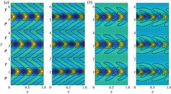
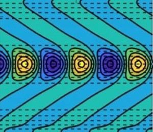
Additionally, we analyse the spatial structure of the fastest growing eigenmode in the presence of ZR. We present in figure 7(a) such spatial structure for the maximum eigenmode corresponding to  $\mathcal {A} = 0.05$ and
 $\alpha = 3$, and include in supplementary material those for
 $\mathcal {A} = 0.1, 0.2$ with
 $\alpha = 1, 3$. Note that, since we solve the coupled eigenproblem, the linear combination of all meridionally coupled eigenmodes at
 $k$ corresponding to the largest growth rate are plotted in each case. Unlike the meridionally uniform eigenmodes (the Philips mode) over the flat bottom, the eigenmodes in the presence of ZR possess meridional variation. These are also localised in regions of negative meridional gradients of topography, where baroclinic instability is expected to be the strongest. Another important aspect is that these eigenmodes have a curved structure and resemble oceanic banana-shaped eddies, which are formed in the vicinity of strong zonal flows (Berloff et al. Reference Berloff, Karabasov, Farrar and Kamenkovich2011; Waterman & Hoskins Reference Waterman and Hoskins2013). This shape in oceanic eddies is result of strong shear due to meridionally varying background zonal flows and the regions of strongest zonal flows also have the largest meridional PV gradients in the upper layer. Similarly, in the presence of ZR, the fastest growing eigenmodes are localised in the regions of strongest meridional PV gradients in the lower layer. It is intriguing that just a presence of variable topography can lead to these banana-shaped eigenmodes, even though the zonal flow is uniform. We suspect that this banana shape is a result of meridional variations in the zonal phase speeds of Rossby waves as the mean PV gradient varies meridionally. In the regions of the strongest meridional PV gradients, zonal phase speeds are expected to be largest from the linear dispersion relation. Hence, the same eddy can experience different zonal phase speeds at different latitudes and this can distort the eddy shape. The same argument can be applied for banana-shaped eddies present on meridionally varying background zonal flows.
Comparison with numerical simulations in the presence of ZR for  $\mathcal {A} = 0.05$ and
 $\alpha =3$: (a) structure of eigenmodes (left and right panels for the top and bottom layers, respectively) corresponding to the maximum growth rate; (b) snapshot of streamfunction field obtained on a
 $1024^{2}$ simulation at approximately 1000 days with parameter values as in table 1 (left and right panels for the top and bottom layers, respectively). Dashed black lines denote topographic slopes and symbols
 $\boldsymbol {P}$ and
 $\boldsymbol {T}$ represent peak and trough regions of topography, respectively. The colour bar range is
 $[min, max]$ from blue to yellow. There are remarkable similarities between the linear solution and numerical simulations, where the differences in spatial structure are attributed to nonlinearities.

For the benefit of the study, we also verified our results by comparing the spatial structure of growing eddies obtained from the linear stability analysis with streamfunction fields born from doubly periodic numerical simulations in a domain size matching our linear stability analysis, and used 1024 grid points in both horizontal directions; presented in figure 7(b). The details of the numerical model can be found in Berloff et al. (Reference Berloff, Karabasov, Farrar and Kamenkovich2011) and Khatri & Berloff (Reference Khatri and Berloff2018). As seen in figure 7, the spatial structure of growing eddies agrees well with our linear stability analysis predictions, as the differences are small, and are attributed to nonlinearities. Also, positive and negative eddies in numerical simulations tend to be shifted slightly to the south and north, respectively (clearly seen in the last panel in figure 7). There is a possibility that cyclonic and anticyclonic eddies move meridionally in response to meridionally varying Coriolis frequency and topographic height. This offset structure of the eddies could be important for secondary instabilities and jet formation; however, studying those effects is out of the scope of the present work.
3.2.3. Meridionally oriented multiple ridges
We now look at the problem in the presence of MR (see figure 2b). Similar to how we dealt with ZR, we solved (2.16b) for all values of  $k$, while fixing the value of
 $\ell$. This is a consequence of zonal wavenumbers being coupled in the eigenproblem. Thus, we plot solutions in the
 $(\omega _i, \ell )$-parameter space, as seen in figure 8. By comparing these solutions with those in figure 3, we can deduce that the magnitude of the maximum growth remains unchanged with MR and always occurs at
 $\ell =0$. Despite this, the distribution of unstable modes shifts towards larger meridional wavenumbers with increasing
 $\alpha$, similar to what occurs in the presence of ZR. For large enough
 $\alpha$, a second peak close to
 $\ell =10$ appears in the growth rate distribution. The magnitude of this peak decreases with
 $\alpha$ and this indicates suppression of instability at these wavenumbers. Moreover, the meridional phase speeds,
 $c^{(y)} = \omega _r/\ell$, of unstable modes can be seen to increase in magnitude with
 $\alpha$ and
 $\mathcal {A}$ (where this increase can be seen by comparing figure 8 with solutions included in supplementary material for
 $\mathcal {A} = 0.2$).
The  $(\omega _i, \ell )$-plot in the presence of MR, with
 $\mathcal {A} = 0.1$ (see table 1 for parameter values). (a–h) Assume
 $\alpha = 1, 3, 5, 10, 15, 20, 25, 30$, respectively (maximum growth remains constant and the distribution of unstable modes shifts towards larger wavenumbers with increasing
 $\alpha$). Meridional phase speeds are shown in the colour bar (magnitude of speeds increase with increasing
 $\ell$ and
 $\alpha$). When
 $\alpha = 15$, a second maximum occurs and weakens with increases in
 $\alpha$.

In figure 9, we analyse how the maximum growth rate at different meridional wavenumbers is affected by the magnitudes of  $\alpha$ and
 $\mathcal {A}$. As mentioned above, the maximum growth rate always occurs at
 $\ell = 0$, and this is further made apparent in figure 9. Even for large
 $\ell$, the growth rate magnitudes look to be similar for different topographic amplitudes and it is not clear how sinusoidal bottom irregularity affects the overall stability. Here, just comparing the maximum growth rate is not sufficient to understand the overall effect of topography on the stability of the system. We discuss this aspect further in the next subsection.
Non-dimensional  $(\alpha , \ell )$-contour plot for the maximum growth rate in the presence of MR. (a–d) Assume
 $\mathcal {A} = 0.05, 0.1, 0.15, 0.2$, respectively. Growth rates are shown in the colour bar (with white referring to zero growth rate) and seem to decrease for larger
 $\ell$ with increasing
 $\mathcal {A}$.

The spatial structure of the fastest growing eddies in the presence of MR is very similar to the fastest growing mode over a flat bottom (the figure is provided in supplementary material). In particular, there appears to be just one prominent wavenumber in the zonal direction, which is controlled by the value of baroclinic Rossby radius. Furthermore, unlike the ZR scenario, there is no localisation of the eigenmode with respect to MR. Similar to our analysis for ZR, we ran numerical simulations to identify differences due to nonlinear contributions. Snapshots for  $\mathcal {A} = 0.05$ and
 $\alpha = 1, 3, 15$ are collected in figure 10 (further details are provided in the figure caption). This demonstrates a clear consistency with our linear stability analysis for small values of
 $\alpha$, suggesting that a zonally varying topography has no notable effects on the spatial structure of the fastest growing eigenmodes (this is limited to zonal background flows only). On the other hand, for
 $\alpha = 15$, some spatial variation in the meridional direction is seen in the meridionally oriented modes and this indicates a presence of reasonably strong signal at a non-zero
 $\ell$. This could be related to the second growth rate peak in figure 8. Thus, the shift in the distribution may affect the spatial structure of the fastest growing eddies over MR; nevertheless, the effect appears to be small. Alternatively, this could be due to the presence of secondary instabilities (Benilov et al. Reference Benilov, Nycander and Dritschel2004) which are not captured by our baroclinic stability analysis. Note that MR is likely to deflect zonal mean flows in the meridional direction and this process is not addressed in our simulations.
Numerical simulations with MR for  $\mathcal {A} = 0.05$, run on a
 $1024^{2}$ grid using parameter values as in table 1: (a) snapshot of streamfunction field for
 $\alpha = 1$; (b) snapshot of streamfunction field for
 $\alpha = 3$; (c) snapshot of streamfunction field for
 $\alpha = 15$. The left (right) snapshot denotes the upper (lower) layer and the colour bar range is
 $[min, max]$ from blue to yellow. Topographic slopes are not illustrated so differences in spatial structure can be easily identified.

3.2.4. Number of unstable modes
In some cases, it may not be sufficient to just examine the maximum growth rate to evaluate the topographic effects on baroclinic instability, e.g. in figure 8, the maximum growth rate remains the same. Hence, it is advisable to examine growth rates of higher eigenmodes. To get a better picture of the extent topography weakens baroclinic instability, we specifically examine the changes in the total number of unstable modes, as well as in the sum of their growth rates for the system. We present this information in figure 11, where the top two panels identify the number of unstable modes as a function of topographic ridges for ZR and MR, respectively, and the bottom two panels display the sum of all unstable growth rates in the system. In the presence of ZR, the number of unstable modes shows a decreasing trend with  $\alpha$. The same is true for the sum of growth rates, which decreases with increasing
 $\mathcal {A}$ as well as
 $\alpha$. Thus, in the overall behaviour, the presence of ZR suppresses the baroclinic instability in the system. We reached the same conclusion when we looked at the maximum growth rate, which also decreases (figure 5).
The number of unstable modes (a,b) and the sum of positive growth rates (c,d) as functions of  $\alpha$: (a,c) in the presence of ZR; (b,d) in the presence of MR.

On the other hand, in the presence of MR, the number of unstable modes first increases up to some small value of  $\alpha$, but the number then mostly decreases. As for the sum of positive growth rates, the general decreasing trend with
 $\alpha$ indicates the suppression of baroclinic instability. This behaviour of increased stability is difficult to infer by just looking at the growth rate of the most unstable modes as the maximum growth rate shows negligible difference (figure 8). The approach discussed in this subsection is rather qualitative and is only used with an intention to make a broader sense of understanding on the effects of the number of ridges and topographic amplitude on the stability of the system.
3.3. Linear stability for a thin-upper-layer case
Despite the choice of equal layer depths being convenient to work with, it is important to investigate how the results from the linear-stability analysis change with distinct layer depths. For this purpose, we repeat our analysis for a configuration which assumes the upper layer has thickness much less than the lower layer (referred to as a thin-upper-layer case). We could equally obtain solutions assuming a thick upper layer, however, this particular regime is not physically relevant as far as the ocean is concerned, and so we do not consider this. It is worth noting that choosing distinct layer depths results in different stratification parameters, hence the critical velocity for baroclinic instability also differs and an inter-comparison of growth rates is not possible. With this in mind, we consider background velocity magnitude,  $\hat {U}$, which is double the respective critical velocity. We followed the same approach in our analysis in the equal-depth configuration, where we had
 $\hat {U}/\hat {U}_c = 5 \ \text {cm} \ \text {s}^{-1}/2.5\ \text {cm}\ \text {s}^{-1} = 2$.
Here, we assume  $\hat {H}_1 = 400$ m and
 $\hat {H}_2 = 3.6$ km for the thin-upper-layer case. The dimensional value of velocity adopted to force the configuration to exhibit baroclinic instability was
 $\hat {U} = 25$ cm s
 $^{-1}$. Also, the magnitudes of stratification parameters in the top and bottom layers change because of unequal layer depths. The value of baroclinic Rossby radius was kept the same, i.e. 25 km, and the rest of the parameter values were as in table 1. In this section, we mainly focus on the effects of ZR on baroclinic instability in model configurations with unequal layer depths. The effects of MR on the stability are very similar as discussed in § 3.2.3, and so we do not focus on this since the differences are negligible.
In the thin-upper-layer case, as seen in figure 12 for  $\mathcal {A} = 0.1$, we notice similarities with equal layer depths, such as eigenmodes shifting towards larger values of
 $k$ with increasing values of
 $\alpha$, as well as depression of maximum growth for
 $\alpha \geq 3$ (though there is an initial spike for
 $\alpha < 3$) and increasing zonal phase speeds. However, some interesting behaviour becomes more evident when
 $\alpha \geq 10$ (d–h). The distribution of unstable eigenmodes separate into two clusters, the first of which for
 $k = (0, 10)$ and the second for
 $k = (10, 20)$. Such cluster separation occurs because the instabilities are connected to either
 $\hat {\lambda }$ (the baroclinic Rossby radius) or
 $\hat {L}_{{Top}}$ (the topographic length scale), and when these scales are distinctly different, we begin to see two isolated branches. In the initial cluster, the maximum growth rate experiences greater depression in comparison with the second cluster maxima with increasing values of
 $\alpha$. Moreover, as
 $k$ increases, the zonal phase speeds in the first cluster increase, while those in the second cluster appear to decrease (albeit the zonal phase speeds in the second cluster are much greater than those present in the first cluster). On the other hand, increasing the value of
 $\alpha$ seemingly reduces zonal phase speeds in the first cluster, while enhancing zonal phase speeds in the second cluster (though this behaviour appears to be weak).
Thin-upper-layer configuration for ZR with  $\mathcal {A} = 0.1$. (a–h) Assume
 $\alpha = 1, 3, 5, 10, 15, 20, 25, 30$, respectively. The maximum growth rate increases for small values of
 $\alpha = 1, 3$ and then decreases in the proceeding panels (
 $\alpha \geq 5$). The distribution splits into two clusters, each having a distinct maximum. The maximum of the first cluster is greatly suppressed with increases in
 $\alpha$ relative to the weakly suppressed second cluster maxima. The zonal phase speeds are shown in the colour bar.

Investigating this behaviour for a larger topographic amplitude of  $\mathcal {A} = 0.2$ (the figure for this is included in supplementary material so the present manuscript remains concise), the initial spike in growth rate is slightly greater than in figure 12, but is depressed when
 $\alpha = 3$ rather than enhanced, as in the
 $\mathcal {A}=0.1$ case (figure 12). Again, the two clusters of unstable modes are formed for
 $\alpha \geq 10$ and the modes in these clusters exhibit similar behaviour to that seen for a smaller value of
 $\mathcal {A}$ (figure 12). One notable difference is that for the larger topographic amplitude case, the two clusters become more disconnected with increasing the value of
 $\alpha$ than seen in figure 12. In addition, the growth rates of eigenmodes present in the first cluster are enhanced by increased topography amplitude, while the growth rates of eigenmodes present in the second cluster are depressed by this increase. One possibility for these differences is that the clusters formed for
 $\mathcal {A} = 0.2$ are present at relatively larger zonal wavenumbers than in figure 12. Despite these differences, the behaviour of zonal phase speeds of eigenmodes in both clusters remains consistent with the characteristics seen in figure 12, with the exception being an enhancement in the value of the zonal phase speed of all eigenmodes.
4. Discussion and conclusions
The primary focus of this investigation was to present a linear stability analysis for oceanic flows in the presence of sinusoidal bottom topography. We excite the system to exhibit baroclinic instability by imposing a zonally uniform background velocity shear in the upper layer of a two-layer fluid. To get an elementary representation of the dynamical behaviours involved, we reduced our model equations to a linear form, from which we obtained an eigenproblem that encoded information concerning unstable growth rates, zonal and meridional phase speeds and spatial structures of perturbation streamfunctions. Topography was assumed to be composed of multiple ridges oriented either along the zonal direction (ZR) or meridional direction (MR) and the eigenproblem solved by varying the number of ridges and various topographic amplitudes. The results in the paper mainly deal with equal layer depths, but a thin-upper-layer configuration with  $\hat {H}_1 = 400$ m is also briefly discussed in the case of ZR.
In accord with the aforementioned studies considering small-scale sinusoidal topography (Benilov Reference Benilov2001; LaCasce et al. Reference LaCasce, Escartin, Chassignet and Xu2019; Radko Reference Radko2020), eigenmodes are found to have maximum growth rates suppressed by ZR (figure 4) and unchanged by MR (figure 8). We observed a shift in the distribution of eigenmodes towards larger wavenumbers and an enhancement in phase speed magnitude with increasing values of  $\alpha$ and
 $\mathcal {A}$ (values considered for non-dimensional topographic wavenumber and amplitude are given in table 1). Moreover, the study by Radko (Reference Radko2020) identified that MR slightly intensifies mesoscale eddies in the upper layer relative to the flat-bottom correspondence, motivating the second peak in figure 8 which takes form when
 $\alpha \geq 15$. The second peak is most pronounced for horizontal topography scales commensurate to
 $2{\rm \pi} \hat {\lambda }$ (
 $\hat {\lambda }$ being the baroclinic Rossby radius as defined in table 1), with the peak being suppressed as
 $\alpha$ increases. Similarly to that observed in Benilov (Reference Benilov2001), flows localised in a thin upper layer experience a weaker stabilisation from the presence of ZR (figure 12). However, a notable finding of this study is unstable modes appearing in two separate clusters (figures 4 and 12) for topographic wavelengths roughly equal to
 $2{\rm \pi} \hat {\lambda }$ (figure 6). This suggests that periodic topography can excite baroclinic instability that is centred around two different length scales instead of just the baroclinic Rossby radius.
To expand on this work, a natural progression would be the consideration of different topographic features. Many studies have already investigated the problem of a topographic slope (Hart Reference Hart1975a,Reference Hartb; Boland et al. Reference Boland, Thompson, Shuckburgh and Haynes2012; Chen & Kamenkovich Reference Chen and Kamenkovich2013; Khatri & Berloff Reference Khatri and Berloff2018; LaCasce et al. Reference LaCasce, Escartin, Chassignet and Xu2019), but more realistic bathymetry would be a combination of spatially localised ridges and isolated mountains. A number of studies have looked into the effects of isolated ridges and mountains on the dynamics in isopycnal layered as well as in primitive equation ocean models and have found evidence of changes in the strength of baroclinic instability on either side of topography (e.g. see Abernathey & Cessi Reference Abernathey and Cessi2014; Youngs et al. Reference Youngs, Thompson, Lazar and Richards2017; Patmore et al. Reference Patmore, Holland, Munday, Naveira Garabato, Stevens and Meredith2019). However, there is no clear sense of understanding how topography affects the primary instability and baroclinic eddies. Also, we only considered zonal background flows in this study. Since topography can affect the orientation and direction of ocean flows, both zonal and meridional background flows could be considered in the future. We believe that the approach used in this work could prove useful in addressing such research questions.
Aside from this, the present study limits attention to a one-dimensional topography as a two-dimensional topography carries a large computational cost. Regardless, it is valuable to expand on works assuming two-dimensional topography since the flow dynamics could potentially be more complicated than what we have identified with a one-dimensional topography. Another obvious limitation of our work is its attention to linear stability only. Even though our linear solutions resemble high resolution numerical simulations, extending this work to a complete nonlinear or quasi-nonlinear analysis is desirable as topographic interactions are strongly affected by the energy cascade (Rhines Reference Rhines1977). Despite frameworks such as shallow-water and primitive equations being better equipped to tackle the small-scale topography problem, it would be interesting to see how our QG results for large-scale topography change in different model regimes for values of  $\alpha$ and
 $\mathcal {A}$ which push the QG limit and deal with topography of shorter wavelength.
Acknowledgement
The authors would like to thank the HPC team at Imperial College London for maintaining the computer clusters.
Funding
J.D. is grateful for support from the Roth scholarship, Imperial College London. P.B. gratefully acknowledges support by the NERC grants NE/R011567/1 and NE/T002220/1, the Leverhulme grant RPG-2019-024 and the Moscow Center for Fundamental and Applied Mathematics (supported by the Agreement of 075-15-2019-1624 with the Ministry of Education and Science of the Russian Federation). H.K. is sponsored through award NA18OAR4320123 from the National Oceanic and Atmospheric Administration, U.S. Department of Commerce. The statements, findings, conclusions, and recommendations are those of the author(s) and do not necessarily reflect the views of the National Oceanic and Atmospheric Administration, or the U.S. Department of Commerce.
Declaration of interests
The authors report no conflict of interest.
Appendix A. Matrix formulation of the eigenvalue problem
Since the eigenproblems are coupled and involve combinations of phase shifted eigenmodes, the system is more complicated than the standard eigenvalue problem. Therefore, we briefly discuss some of the details regarding solving this system of equations in this appendix for completeness.
We can rewrite the eigenproblems (2.16a) and (2.16b) in the matrix form
 \begin{equation} \mathcal{M} \boldsymbol{\phi} = \omega\mathcal{N} \boldsymbol{\phi}, \end{equation}
where we define the eigenvector
 \begin{equation} \boldsymbol{\phi} = \begin{bmatrix} \phi_1(k, -N/2) \\ \phi_1(k, -N/2 + 1) \\ \vdots \\ \phi_1(k, N/2 - 1) \\ \phi_1(k, -N/2) \\ \vdots \\ \phi_2(k, N/2 - 1) \end{bmatrix}\quad \text{or} \quad \boldsymbol{\phi} = \begin{bmatrix} \phi_1(-N/2, \ell) \\ \phi_1(-N/2 + 1, \ell) \\ \vdots \\ \phi_1(N/2 - 1, \ell) \\ \phi_1(-N/2, \ell) \\ \vdots \\ \phi_2(N/2 - 1, \ell) \end{bmatrix}, \end{equation}
for ZR or MR, respectively. In this study, we solve the ZR and MR systems for combinations of  $\mathcal {A} = 0.05, 0.1, 0.15, 0.2$ and
 $\alpha = 1, 3, 5, 10, 15, 20, 25, 30, 40$. If, for simplicity, we limit our attention to ZR with a single ridge, i.e.
 $\alpha = 1$, then the matrix
 $\mathcal {M}$ has the block matrix composition
 \begin{equation} \mathcal{M} = k\begin{bmatrix} \mathcal{M}_1 \\ \mathcal{M}_2 \end{bmatrix}, \end{equation}
where  $\mathcal {M}_1$ is the
 $N \times 2N$ matrix
 \begin{align} \begin{bmatrix} \beta - (k^{2} + \ell_1^{2})U & 0 & \ddots & 0 & S_1U & 0 & \ddots & 0 \\ 0 & \beta - (k^{2} + \ell_2^{2})U & \ddots & 0 & 0 & S_1U & \ddots & 0 \\ \ddots & \ddots & \ddots & \ddots & \ddots & \ddots & \ddots & \ddots \\ 0 & 0 & \ddots & \beta - (k^{2} + \ell_N^{2})U & 0 & 0 & \ddots & S_1U \end{bmatrix}, \end{align}
with  $\ell _j = -N/2 + j - 1$ for
 $j = 1, 2, \ldots , N$, and
 $\mathcal {M}_2$ is the
 $N \times 2N$ matrix
 \begin{equation} \begin{bmatrix} 0 & 0 & \ddots & 0 & \beta - S_2U & \hat{H}\mathcal{A}/2\hat{H}_2 & 0 & \ddots & 0 \\ 0 & 0 & \ddots & 0 & \hat{H}\mathcal{A}/2\hat{H}_2 & \beta - S_2U & \hat{H}\mathcal{A}/2\hat{H}_2 & \ddots & 0 \\ \ddots & \ddots & \ddots & \ddots & \ddots & \ddots & \ddots & \ddots & \ddots \\ \end{bmatrix}, \end{equation}
where the right half of  $\mathcal {M}_2$ is tridiagonal. In a similar manner, the matrix
 $\mathcal {N}$ can be expressed in the block form
 \begin{equation} \mathcal{N} = \begin{bmatrix} \mathcal{N}_1 \\ \mathcal{N}_2 \end{bmatrix}, \end{equation}
with  $\mathcal {N}_1$ being the
 $N \times 2N$ matrix
 \begin{align} \begin{bmatrix} -(k^{2} + \ell_1^{2} + S_1) & 0 & \ddots & 0 & S_1 & 0 & \ddots & 0 \\ 0 & -(k^{2} + \ell_2^{2} + S_1) & \ddots & 0 & 0 & S_1 & \ddots & 0 \\ \ddots & \ddots & \ddots & \ddots & \ddots & \ddots & \ddots & \ddots \\ 0 & 0 & \ddots & -(k^{2} + \ell_N^{2} + S_1) & 0 & 0 & \ddots & S_1 \end{bmatrix}, \end{align}
and  $\mathcal {N}_2$ is the
 $N \times 2N$ matrix
 \begin{align} \begin{bmatrix} S_2 & 0 & \ddots & 0 & -(k^{2} + \ell_1^{2} + S_2) & 0 & \ddots & 0 \\ 0 & S_2 & \ddots & 0 & 0 & -(k^{2} + \ell_2^{2} + S_2) & \ddots & 0 \\ \ddots & \ddots & \ddots & \ddots & \ddots & \ddots & \ddots & \ddots \\ 0 & 0 & \ddots & S_2 & 0 & 0 & \ddots & -(k^{2} + \ell_N^{2} + S_2) \end{bmatrix}. \end{align}
For our purposes, we solve this system of equations for  $k = -N/2, -N/2 + 1,\ldots , N/2 - 1$ and
 $\mathcal {A} = 0.05, 0.1, 0.15, 0.2$.
It is worth noting that this is only the specific configuration for a single topographic ridge. However, since the phase shift in the eigenmodes is due to the presence of  $\alpha$, increasing the number of ridges only involves permuting entries in the matrix
 $\mathcal {M}$ and multiplying the value of
 $\mathcal {A}$ by
 $\alpha$ (the matrix
 $\mathcal {N}$ is the same for all values of
 $\alpha$ as it does not depend on the number of ridges). If we instead consider MR, then the procedure is similar, but we fix
 $\ell$ instead of
 $k$.