1 Introduction
Three-dimensional (3D), turbulent, bottom-propagating density currents that arise due to the spreading of a heavier fluid into a lighter ambient fluid is of common occurrence in the atmosphere and in the oceans. These density currents play an important role in dictating atmospheric pollution, transport of airborne contaminants, ocean mixing and climate dynamics. The heavy fluid, as it propagates into the ambient fluid, entrains and mixes with the lighter ambient fluid, resulting in significant changes in the properties of the current. Knowledge of the front location, reduced gravity and the dynamics of mixing are very important. The bottom surface on which these currents propagate is invariably rough in nature, and cannot be approximated as a smooth surface. More importantly, the type of roughness significantly influences the characteristics and dynamics of these 3D turbulent currents. Roughness introduces significant complexities in the physics, as well as the measurement techniques, and hence not much is understood of dense currents over roughness.
The problem considered in this research is the finite-volume release of a dense fluid into a lighter environment confined in a channel with rigid walls and a bottom wall covered with 3D regular roughness elements. This is the classical lock-exchange flow. The lock-exchange configuration has served as a canonical platform for both numerical and laboratory experiments to study gravity currents (Simpson Reference Simpson1972; Simpson & Britter Reference Simpson and Britter1979; Hacker, Linden & Dalziel Reference Hacker, Linden and Dalziel1996; Shin, Dalziel & Linden Reference Shin, Dalziel and Linden2004; Özgökmen, Iliescu & Fischer Reference Özgökmen, Iliescu and Fischer2009).
In a lock-exchange flow, a vertical barrier in a channel separates two fluids of different densities. The density difference between the heavy and lighter ambient fluids is small, and the Boussinesq approximation holds. Initially, the heavy fluid in the lock has stored potential energy, specified by the height of the lock. With the removal of the lock, the heavy lock fluid carrying the potential energy forms a well-defined frontal region after an initial transience. Beyond the short accelerating transient regime, the currents propagate with a constant velocity, referred to as the slumping regime (Britter & Simpson Reference Britter and Simpson1978; Rottman & Simpson Reference Rottman and Simpson1983). The current moves horizontally, entraining the ambient fluid and growing spatially. From Benjamin’s classical theory (Benjamin Reference Benjamin1968), the most important characteristic feature of the current is the well-defined and distinctive head at the intruding end of the current, which is deeper than the rest of the current. The role of the head region in mixing processes has been clearly demonstrated by Simpson & Britter (Reference Simpson and Britter1979). In lock-exchange flows, the head carries with it a fraction of the initial buoyancy in the lock, and this fraction is dictated by the lock aspect ratio (the ratio of the height to the length of the lock). At the top of the head region, strong Kelvin–Helmholtz (KH) billows form; these break down behind the head, causing strong mixing in the current, so that the interface becomes unstable towards the rear of the head. McElwaine’s theory (McElwaine Reference McElwaine2005) and particle image velocimetry measurements by Kneller, Bennett & McCaffrey (Reference Kneller, Bennett and McCaffrey1999), Thomas, Dalziel & Marino (Reference Thomas, Dalziel and Marino2003) and Samasiri & Woods (Reference Samasiri and Woods2015) indicate a strong mixing at the interface near the head of the current. Recently, Bhaganagar (Reference Bhaganagar2017) used large-eddy simulations (LES) to calculate mixing or entrainment coefficients as the fraction of the volume of the ambient fluid that enters the head due to shear instability generated at the current interface. An alternative way to quantify the entrainment in density currents is by using the concept of available potential energy introduced by Winters et al. (Reference Winters, Lombard, Riley and D’Asaro1995), and which has been successfully used to study the mixing processes (Prastowo et al. Reference Prastowo, Griffiths, Hughes and Hogg2009; Hughes & Linden Reference Hughes and Linden2016; Micard et al. Reference Micard, Dossmann, Gostiaux and Venaille2016).
Density currents over idealized smooth beds are well understood; however, the effect of bed roughness on the dynamics of lock-exchange currents needs clarification. Experimental and numerical data have contributed to our understanding of the effect of surface roughness on front characteristics (La Rocca et al. Reference La Rocca, Adduce, Sciortino and Pinzon2008; Özgökmen & Fischer Reference Özgökmen and Fischer2008; Adduce et al. Reference Adduce, Lombardi, Sciortino and Morganti2009; Tokyay, Constantinescu & Meiburg Reference Tokyay, Constantinescu and Meiburg2011; Nogueira et al. Reference Nogueira, Adduce, Alves and Franca2014; Yuksel Ozan, Constantinescu & Hogg Reference Yuksel Ozan, Constantinescu and Hogg2015), detailed flow descriptions of the changes in the structure of the current as they interact with roughness (Gonzalez-Juez, Meiburg & Constantinescu Reference Gonzalez-Juez, Meiburg and Constantinescu2009; Gonzalez-Juez et al. Reference Gonzalez-Juez, Meiburg, Tokyay and Constantinescu2010; Bhaganagar Reference Bhaganagar2014; Tokyay & Constantinescu Reference Tokyay and Constantinescu2015), time-averaged mixing properties of the current (Negretti, Zhu & Jirka Reference Negretti, Zhu and Jirka2008; Tanino & Nepf Reference Tanino and Nepf2008; Cenedese, Nokes & Hyatt Reference Cenedese, Nokes and Hyatt2017) and flow visualization studies (Peters & Venart Reference Peters and Venart2000). In light of these previous studies, it is clear that surface roughness enhances the wall shear stress, and thus alters the flow characteristics in the frontal region. Density currents over rough surfaces have higher deceleration and faster dilution. Though the experimental studies have contributed to our understanding of the front velocity and structure of the current over roughness, unfortunately, not much knowledge is available on the temporal evolution of the currents and the mixing processes. In particular, it is not clear if the dilution occurs throughout the slumping regime or not.
In density currents, the primary source of mixing is the KH rollers, as the shear results in mixing at the interface. The question still remains as to how the wall shear generated near the roughness influences the primary mixing mechanisms. Furthermore, what is the contribution of the shear generated at the roughness elements in relation to the primary shearing mechanism at the interface? Field data collected by Fernandez & Imberger (Reference Fernandez and Imberger2006) demonstrated that entrainment is mainly dependent on the stress generated at the bottom, directly determined by the roughness and the current properties. The effect of roughness on density current front evolution and mixing is very significant; however, our understanding on mixing in density currents over 3D roughness is still very limited. In particular, the instantaneous mixing process during the slumping regime is still not clear, and the role of local roughness features in diluting the current has not been quantified.
The effect of surface roughness on the flow is very complicated, as roughness geometrical metrics including roughness height, shape and distribution influence the near-wall flow dynamics. In the near-wall region of turbulent flows, as viscosity is important, the relevant velocity scale is the friction velocity
 $u_{\unicode[STIX]{x1D70F}}=\sqrt{\unicode[STIX]{x1D70F}_{w}/\unicode[STIX]{x1D70C}}$
. For wall-bounded, constant-density turbulent flows, high-resolution numerical and experimental studies quantified the role of wall shear stress due to uniform and irregular blocks of roughness in terms of
 $u_{\unicode[STIX]{x1D70F}}$
(Bhaganagar, Kim & Coleman Reference Bhaganagar, Kim and Coleman2004; Wu & Christensen Reference Wu and Christensen2010; Bhaganagar & Chau Reference Bhaganagar and Chau2015). Similarly, the near-wall region of the density current has a significant role in modifying the flow dynamics, and in particular the wall shear stress (
 $\unicode[STIX]{x1D70F}_{w}$
), which manifests itself as a mean velocity gradient at the wall and dictates the frictional drag encountered by the current. The local Reynolds number based on the friction velocity can be defined as
 $Re_{\unicode[STIX]{x1D70F}}=u_{\unicode[STIX]{x1D70F}}h_{H}/\unicode[STIX]{x1D708}$
, based on local current height
 $(h_{H})$
. In this study, we characterize the instantaneous wall shear stress in terms of
 $Re_{\unicode[STIX]{x1D70F}}$
. There is evidence that enhanced wall shear stress dilutes the current and manifests as enhanced entrainment. High-resolution LES were used by Tokyay, Constantinescu & Meiburg (Reference Tokyay, Constantinescu and Meiburg2012) to demonstrate that two-dimensional (2D) dunes entrain higher than 2D ribs of comparable size and relate the time evolution of
 $u_{\unicode[STIX]{x1D70F}}$
to entrainment.
The early works of Nikuradse (Reference Nikuradse1933) and the classical experiments of Schlichting (Reference Schlichting1936) used roughness height and the spacing between the roughness elements to classify roughness. Recent experimental (Schultz & Flack Reference Schultz and Flack2009; Wu & Christensen Reference Wu and Christensen2010) and numerical data (Orlandi & Leonardi Reference Orlandi and Leonardi2006; Chau & Bhaganagar Reference Chau and Bhaganagar2012; De Marchis & Napoli Reference De Marchis and Napoli2012) on constant-density turbulent flows over roughness revealed new insights on roughness parameters that influence the wall shear stress. Roughness volume fraction (the ratio of the volume occupied by roughness to the volume of the surrounding fluid) and roughness solidity (the ratio of the total frontal area of the roughness in relation to the base area) have emerged as reliable metrics to quantify the wall shear stress due to roughness geometry (Lettau Reference Lettau1969; Counehan Reference Counehan1971; Macdonald, Griffiths & Hall Reference Macdonald, Griffiths and Hall1998; Flack & Schultz Reference Flack and Schultz2014). Hence, in this study, the density currents are studied within the context of roughness solidity and volume fraction.
Only in the recent literature have data on instantaneous entrainment started to appear. Analysis of density currents over smooth surfaces from experimental measurements and high-resolution LES studies (e.g. Ottolenghi et al. Reference Ottolenghi, Adduce, Inghilesi, Armenio and Roman2016; Bhaganagar Reference Bhaganagar2017) have revealed that entrainment is a highly unsteady process and dilution of the current starts as early as the beginning of the slumping regime. Fragoso, Patterson & Wettlaufer (Reference Fragoso, Patterson and Wettlaufer2013) used highly spatially resolved optical based experiments to study the temporal entrainment during the slumping regime, and provided some of the first evidence that mixing in the head of a density current starts during the early stages of the slumping regime. Data on density currents over rough surfaces is even more sparse. The few available data for the current over surface roughness include the experimental data by Wilson, Friedrich & Stevens (Reference Wilson, Friedrich and Stevens2017) for isolated roughness and by Nogueira et al. (Reference Nogueira, Adduce, Alves and Franca2014) for a sediment bed. In the latter study, the temporal evolution of current depth-averaged density was analysed to demonstrate roughness results in significant dilution during the beginning of the slumping regime. The present investigation is one of the first studies to use highly resolved data to explore the instantaneous mixing processes in the density current over 3D roughness elements. We focus on 3D regular roughness elements, including cubes, pyramids, combinations of cubes and pyramids consisting of both cases with identical roughness elements and with elements consisting of random height distribution. The maximum height of the roughness elements is 10 % of the lock height, and the elements are well immersed within the current.
In this paper, the following research questions will be addressed.
-
(i) For the same initial conditions of the lock, what are the differences in the front characteristics over a rough wall compared to a smooth wall? In particular, what are the differences that arise due to difference in roughness shape (i.e. cubes versus pyramid shape), and what are the differences that arise due to difference in identical versus random arrangement of roughness elements with the same mean height of roughness and centre–centre spacing between the roughness elements? Differences in cubes/pyramids and uniform/random height introduce differences in roughness metrics, such as volume fraction of roughness and area ratio of roughness.
-
(ii) How does roughness affect the instantaneous mixing in the density current? How does the instantaneous entrainment and mixing during the slumping and inertial regimes of density currents depend on the roughness? This is connected to an understanding of the role of wall shear stress versus the shear at the interface due to KH instability that contributes to entrainment of ambient fluid into the current. This is also related to the question: Is the modified flow dynamics and the consequences of mixing due to the differences in the roughness configuration represented by friction Reynolds number (
 $Re_{\unicode[STIX]{x1D70F}}$
)?

The paper is arranged as follows. The physical problem with the simulation domain and the boundary conditions considered in this analysis is presented in § 2.1. We use a finite-volume LES methodology with a Boussinesq approximation to solve the 3D nonlinear Navier–Stokes (NS) momentum equations and scalar transport equation. The subgrid scales are modelled using the dynamic Smagorinsky eddy viscosity model. Roughness is introduced using a penalization approach by solving the Darcy–Brinkman equation, where, in the limiting case of permeability approaching zero/infinity, the domain mimics solid/fluid regions. The details of the NS formulation and the approach to mimic the roughness are explained in §§ 2.2 and 2.3, respectively. The front characteristics and the definitions to quantify the current are explained in § 2.4. The results are presented in § 3, flow regimes and the associated analysis is discussed in §§ 3.1–3.4, shear stress results are discussed in § 3.5, and finally the entrainment and mixing are discussed in § 3.6. In § 4, we present the conclusions.
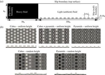
(a) Schematic of the computational domain for lock-exchange release system with lock of height
 $h_{0}$
and length
 $5h_{0}$
. The roughness elements are placed on the lower wall of the channel. (b) The five rough-wall cases that are considered in this work. The roughness elements comprise cubes, pyramids and combinations of cubes and pyramids of uniform elevation (top row), and cubes and pyramids with random elevation (bottom row). For all the cases the mean roughness height is
 $0.1h_{0}$
.

2 Problem formulation and numerical approach
2.1 Simulation domain and boundary conditions
The physical problem considered is a horizontal channel with the lower wall dotted by bottom-mounted roughness elements; the upper wall is a fixed rigid wall, as shown in figure 1(a). The problem at hand is a full lock release case, where the lock height is the same as the height of the channel (
 $h_{0}$
). Initially, the heavy fluid fills the lock of length
 $L_{0}$
(
 $L_{0}=5h_{0}$
). The lock aspect ratio (
 $L_{0}/h_{0}$
) is 5. The streamwise and spanwise extents of the domain are
 $40h_{0}$
and
 $2.5h_{0}$
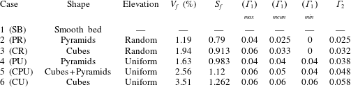
, respectively. In this work, the rough wall consists of 3D regular roughness elements with a fixed distribution of roughness features that are in the shapes of cubes and pyramids having uniform and random heights. We will refer to the distribution of roughness with uniform elevation as uniform roughness, and the distribution with random elevations as random roughness. Figure 1(b) shows the top and front views for the different cases that are considered in this study. The cases consist of identical cube-shaped roughness elements that are referred to as ‘uniform cubes’, identical pyramid-shaped roughness elements that are called ‘uniform pyramids’, combinations of both cubes and pyramids of uniform height, which are referred to as ‘uniform cubes and pyramids’, cubes with random height distribution referred to as ‘random cubes’, and pyramids with random height distribution referred to as ‘random pyramids’. Definitions of roughness metrics, listed in table 1, include the following.
-
(i) Volume fraction
$(V_{f})$
, (2.1)where
$$\begin{eqnarray}V_{f}=\frac{\displaystyle \mathop{\sum }_{i=1}^{390}V_{i}^{R}}{V_{0}},\end{eqnarray}$$
$V_{i}^{R}$
is the volume of the
$i$
th roughness feature and
$V_{0}$
is the volume of the simulation domain.
-
(ii) Surface fraction
$(S_{f})$
, (2.2)where
$$\begin{eqnarray}S_{f}=\frac{\displaystyle A_{i}^{R}}{A_{b}},\end{eqnarray}$$
$A_{i}^{R}$
is the total surface area of the
$i$
th roughness feature and
$A_{b}$
is the area of unoccupied bottom bed. Surface fraction
$(S_{f})$
is unique for each case and exercises a direct influence on bottom shear experienced by the advancing current.
-
(iii) Streamwise solidity
$(\unicode[STIX]{x1D6E4}_{1})$
, (2.3)where
$$\begin{eqnarray}\unicode[STIX]{x1D6E4}_{1}=\frac{\displaystyle A_{j}^{P}}{l_{span}h_{0}},\end{eqnarray}$$
$A_{j}^{P}$
is the area of the
$j$
th row of roughness features when projected on the right (slip) wall of the domain,
$h_{0}$
is the channel height and
$l_{span}$
is the length of the span. Thus
$\unicode[STIX]{x1D6E4}_{1}$
represents the solidity (Schlichting Reference Schlichting1936; Jimenez Reference Jimenez2004; Flack & Schultz Reference Flack and Schultz2014) normal to the channel span. It is constant when roughness shapes and heights remain unchanged (cases 4 and 6) but fluctuates with variation in either one of them (cases 2, 3 and 5). Therefore, we present the maximum
$(\unicode[STIX]{x1D6E4}_{1})_{max}$
, mean
$(\unicode[STIX]{x1D6E4}_{1})_{mean}$
and minimum
$(\unicode[STIX]{x1D6E4}_{1})_{min}$
values for
$\unicode[STIX]{x1D6E4}_{1}$
. The zero entries for
$(\unicode[STIX]{x1D6E4}_{1})_{min}$
in cases 1 and 2 convey that randomness in the feature heights lead to a smooth surface in certain stretches of the bottom wall.
-
(iv) Spanwise solidity
$(\unicode[STIX]{x1D6E4}_{2})$
, (2.4)where
$$\begin{eqnarray}\unicode[STIX]{x1D6E4}_{2}=\frac{\displaystyle \mathop{\sum }_{j=1}^{78}A_{j}^{S}}{Lh_{0}},\end{eqnarray}$$
$A_{j}^{S}$
is the area of the
$j$
th row of roughness features when projected on the front (periodic) boundary of the domain. Thus
$\unicode[STIX]{x1D6E4}_{2}$
represents solidity normal to the channel length
$(L=40h_{0})$
. Like
$S_{f}$
,
$\unicode[STIX]{x1D6E4}_{2}$
is constant and unique for each roughness case.


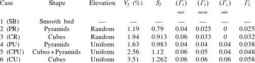
The case studies considered have the same maximum roughness height
 $(k)$
, streamwise spacing
 $\unicode[STIX]{x1D706}_{x}=5k$
and spanwise spacing
 $\unicode[STIX]{x1D706}_{z}=5k$
between the roughness elements. The maximum roughness height is the same for all cases, and is considered to be 10 % of the lock height. The volume fraction is different for each case, and it varies from the greatest for uniform cubes (3.51 %) to the smallest (1.19 %) for pyramids with random roughness. All cases have the same ratio of the total plan area of the obstacles to the lower wall area. The cases have different ratios of the total frontal area of the obstacles to the total area, because, though the cases with uniform pyramids and cubes have the same plan area, roughness height and spacing between the obstacles, the obstacles have different total frontal areas. The differences between the uniform cubes versus the random cubes or uniform pyramids versus random pyramids is the difference in variation of solidity. The case with combination of uniform cubes and pyramids has a different total frontal area and solidity.
2.2 Governing equations
A finite-volume LES implementation, with penalization-function-type immersed-boundary method to realize the bottom mounted obstacle geometry, has been used to simulate turbulent density currents. The governing equations are the following filtered NS system of equations, under Boussinesq approximation (filtered variables are denoted by overbar).
-
(i) Continuity equation:
(2.5)
$$\begin{eqnarray}\unicode[STIX]{x1D735}\boldsymbol{\cdot }\overline{\boldsymbol{u}}=0.\end{eqnarray}$$
-
(ii) Momentum equation:
(2.6)where
$$\begin{eqnarray}\frac{\unicode[STIX]{x2202}\overline{\boldsymbol{u}}}{\unicode[STIX]{x2202}t}+\overline{\boldsymbol{u}}\boldsymbol{\cdot }\unicode[STIX]{x1D735}\overline{\boldsymbol{u}}=-\frac{\unicode[STIX]{x1D735}\overline{p}}{\unicode[STIX]{x1D70C}}+\unicode[STIX]{x1D708}\unicode[STIX]{x1D6FB}^{2}\overline{\boldsymbol{u}}+\unicode[STIX]{x1D735}\boldsymbol{\cdot }\{(\unicode[STIX]{x1D708}+\unicode[STIX]{x1D708}_{t})[\unicode[STIX]{x1D735}\overline{\boldsymbol{u}}+(\overline{\boldsymbol{u}})^{\text{T}}]\}+\overline{\unicode[STIX]{x1D70C}}\boldsymbol{g}+\overline{\boldsymbol{f}},\end{eqnarray}$$
$\overline{\unicode[STIX]{x1D70C}}$
represents the resolved relative density field and
$\overline{\boldsymbol{f}}$
is a source term, which will be discussed in detail in § 2.3. The third term on the right-hand side results from applying the spatial filter to the convection term in the NS equation and invoking the Boussinesq hypothesis of a linear stress–strain relationship. Finally,
$\unicode[STIX]{x1D708}_{t}$
represents the eddy viscosity, which is calculated from the dynamic Smagorinsky model proposed by Germano et al. (Reference Germano, Piomelli, Moin and Cabot1991).
-
(iii) Transport equation:
(2.7)where
$$\begin{eqnarray}\frac{\unicode[STIX]{x2202}\overline{\unicode[STIX]{x1D70C}}}{\unicode[STIX]{x2202}t}+\unicode[STIX]{x1D735}(\overline{\unicode[STIX]{x1D70C}}\overline{\boldsymbol{u}_{j}})=\unicode[STIX]{x1D735}(\unicode[STIX]{x1D705}_{eff}\unicode[STIX]{x1D735}\overline{\unicode[STIX]{x1D70C}}),\end{eqnarray}$$
$\unicode[STIX]{x1D705}_{eff}=\unicode[STIX]{x1D708}_{t}/Sc_{t}+\unicode[STIX]{x1D708}_{0}/Sc$
.



The solver executes the ‘pressure-implicit with splitting of operators’ (PISO) algorithm to evaluate the momentum flux. PISO decouples the pressure and velocity fields by splitting the operators into implicit predictor and multiple explicit corrector steps. Furthermore, the convective term is linearized by using the convective velocity from the previous time step. Time integration is undertaken using a second-order-accurate bounded three-point backward scheme. Convective terms are handled with a bounded Gauss self-filtered central difference (SFCD) scheme, diffusion terms are handled using a Gauss scheme with linear interpolation, and scalar transport is calculated using a Gauss–Vanleer scheme.
2.3 Penalization method
A volume-penalization-based immersed-boundary method is used to realize the roughness topology on a pure Cartesian mesh. This approach is a special case of feedback forcing procedure (Goldstein, Handler & Sirovich Reference Goldstein, Handler and Sirovich1993); however, here the solid regions are manifested as a porous medium with vanishing permeability (Angot, Bruneau & Fabrie Reference Angot, Bruneau and Fabrie1999). The fields in the time-discretized momentum equation are replaced with penalized quantities
 $\boldsymbol{u}_{\unicode[STIX]{x1D702}}$
and
 $p_{\unicode[STIX]{x1D702}}$
such that
 $\boldsymbol{u}_{\unicode[STIX]{x1D702}}=\overline{\boldsymbol{u}}+\unicode[STIX]{x1D702}\widetilde{\boldsymbol{u}}$
and
 $p_{\unicode[STIX]{x1D702}}=\overline{p}+\unicode[STIX]{x1D702}\widetilde{p}$
. The symbol
 $\unicode[STIX]{x1D702}$
represents the penalization parameter
 $(\unicode[STIX]{x1D702}\ll 1)$
. Therefore, as
 $\unicode[STIX]{x1D702}\rightarrow 0$
, the penalized velocity field
 $\boldsymbol{u}_{\unicode[STIX]{x1D702}}\rightarrow \overline{\boldsymbol{u}}$
and error
 $\widetilde{\boldsymbol{u}}\rightarrow 0$
:
 $$\begin{eqnarray}\frac{\unicode[STIX]{x2202}\boldsymbol{u}_{\unicode[STIX]{x1D702}}}{\unicode[STIX]{x2202}t}+\boldsymbol{u}_{\unicode[STIX]{x1D702}}\boldsymbol{\cdot }\unicode[STIX]{x1D735}\boldsymbol{u}_{\unicode[STIX]{x1D702}}=-\frac{\unicode[STIX]{x1D735}p_{\unicode[STIX]{x1D702}}}{\unicode[STIX]{x1D70C}}+\unicode[STIX]{x1D708}\unicode[STIX]{x1D6FB}^{2}\boldsymbol{u}_{\unicode[STIX]{x1D702}}+\unicode[STIX]{x1D735}\boldsymbol{\cdot }\{(\unicode[STIX]{x1D708}+\unicode[STIX]{x1D708}_{t})[\unicode[STIX]{x1D735}\boldsymbol{u}_{\unicode[STIX]{x1D702}}+(\unicode[STIX]{x1D735}\boldsymbol{u}_{\unicode[STIX]{x1D702}})^{\text{T}}]\}+\overline{\unicode[STIX]{x1D70C}}\boldsymbol{g}-\frac{\unicode[STIX]{x1D712}}{\unicode[STIX]{x1D702}}\boldsymbol{u}_{\unicode[STIX]{x1D702}}+\overline{\boldsymbol{f}}.\end{eqnarray}$$
Equation (2.8) is defined over a heterogeneous domain
 $(\unicode[STIX]{x1D6FA})$
comprising fluid region
 $\unicode[STIX]{x1D6FA}_{f}$
and solid region
 $\unicode[STIX]{x1D6FA}_{s}$
such that
 $\unicode[STIX]{x1D6FA}_{f}\cup \unicode[STIX]{x1D6FA}_{s}=\unicode[STIX]{x1D6FA}$
and
 $\unicode[STIX]{x1D6FA}_{f}\cap \unicode[STIX]{x1D6FA}_{s}=\emptyset$
. The boundary between
 $\unicode[STIX]{x1D6FA}_{f}$
and
 $\unicode[STIX]{x1D6FA}_{s}$
is denoted by
 $\unicode[STIX]{x1D6E4}$
. The second last term in (2.8) is introduced into momentum equation (2.6) to account for the heterogeneous nature of the domain; here
 $\unicode[STIX]{x1D712}$
represents a masking function that distinguishes solid and fluid regions,
 $$\begin{eqnarray}\displaystyle & \unicode[STIX]{x1D712}=0\quad \forall \,\boldsymbol{x}\in \unicode[STIX]{x1D6FA}_{f}, & \displaystyle\end{eqnarray}$$
 $$\begin{eqnarray}\displaystyle & \unicode[STIX]{x1D712}=1\quad \forall \,\boldsymbol{x}\in \unicode[STIX]{x1D6FA}_{s}. & \displaystyle\end{eqnarray}$$
Substituting the definitions of
 $\boldsymbol{u}_{\unicode[STIX]{x1D702}}$
and
 $p_{\unicode[STIX]{x1D702}}$
in (2.8) and identifying terms of the same order, for
 $\unicode[STIX]{x1D6FA}_{s}$
, leaves us with
 $$\begin{eqnarray}\frac{\unicode[STIX]{x1D735}\overline{p}}{\unicode[STIX]{x1D70C}}+\frac{\boldsymbol{u}_{\unicode[STIX]{x1D702}}-\overline{\boldsymbol{u}}}{\unicode[STIX]{x1D702}}+\overline{\unicode[STIX]{x1D70C}}\boldsymbol{g}=\,\overline{\boldsymbol{f}}\quad \forall \,\boldsymbol{x}\in \unicode[STIX]{x1D6FA}_{s}.\end{eqnarray}$$
Therefore, if
 $\unicode[STIX]{x1D6FA}_{s}$
is interpreted as a porous medium, given that no additional external force is active (i.e.
 $\overline{\boldsymbol{f}}=0$
and
 $\overline{\unicode[STIX]{x1D70C}}\boldsymbol{g}=0$
), the penalization parameter
 $(\unicode[STIX]{x1D702})$
will correspond to its permeability
 $(K)$
. Furthermore, as
 $\unicode[STIX]{x1D702}\rightarrow 0$
the permeability of the porous medium will diminish; asymptotically we realize a rigid solid. A similar analysis for
 $(\unicode[STIX]{x1D6FA}_{f})$
retrieves the momentum equation in its native form (2.6). Angot et al. (Reference Angot, Bruneau and Fabrie1999) conveyed that a priori estimation of penalized velocity, subject to an incompressibility constraint, results in a penalized velocity field
 $(\boldsymbol{u}_{\unicode[STIX]{x1D702}})$
that converges towards fluid velocity
 $(\boldsymbol{u})$
as
 $\unicode[STIX]{x1D702}\rightarrow 0$
. In numerical simulations this estimation can be passed as initial conditions to the solver. Introducing the velocity term of Darcy’s equation (an empirical relation governing flows through porous media) as a forcing term coupled with masking function
 $\unicode[STIX]{x1D712}$
in the momentum equation allows the forcing to vanish in the fluid region
 $(\unicode[STIX]{x1D712}=0)$
and activate only within the solid region
 $(\unicode[STIX]{x1D712}=1)$
. The forcing term introduces excessive volumetric drag on account of
 $K\rightarrow 0$
, thus bringing momentum flux across the solid region down to machine precision. Consequently, the convection terms cease to influence the momentum transport. Left with time derivative, diffusion term, pressure gradient and the forcing term (in the form of Darcy’s law), we realize Brinkman’s (Reference Brinkman1949) formulation for simulating flow through a porous medium.
Cases reported in this work comprise roughness features in the shape of cubes and stepped pyramids. At this point focus is laid on geometric simplicity, so both shapes mentioned above can be realized by simply combining orthogonal hexahedral control volumes in sequential arrays. Each feature thus comprises an integer multiple of control volume cells. The control volumes comprising roughness features are referenced in a cell-zone data structure and passed on to the solver. For these control volumes the solver assigns
 $\unicode[STIX]{x1D712}=1$
while evaluating momentum flux. The forcing term emulates the left-hand side of Darcy’s law. To accommodate higher Reynolds numbers, the Forchheimer correction (Forchheimer Reference Forchheimer1901) has been applied to Darcy’s law. Therefore,
 $$\begin{eqnarray}\overline{\boldsymbol{f}}=-\left[\unicode[STIX]{x1D707}\unicode[STIX]{x1D63F}+{\textstyle \frac{1}{2}}\unicode[STIX]{x1D70C}|\overline{\boldsymbol{u}}|\unicode[STIX]{x1D641}\right]\overline{\boldsymbol{u}},\end{eqnarray}$$
where
 $\unicode[STIX]{x1D63F}=1/\unicode[STIX]{x1D612}_{ij}$
and
 $\unicode[STIX]{x1D641}=2C_{E}/\sqrt{\unicode[STIX]{x1D612}_{ij}}$
. The permeability tensor
 $\unicode[STIX]{x1D612}_{ij}$
is a free parameter specified by the user; under the isotropic assumption it transforms to a constant scalar and consequently
 $\unicode[STIX]{x1D60B}_{ij}$
and
 $\unicode[STIX]{x1D60D}_{ij}$
also manifest as constant scalars. Ergun’s constant
 $C_{E}$
(Ergun Reference Ergun1952) is derived from empirical relations. For our problem formulation, we directly define
 $D$
and
 $F$
to be of the order of
 $10^{20}$
. This number is arrived at after conducting sensitivity tests; at this order and beyond, the volume-averaged velocity within the porous medium is recorded to be of the order of
 $10^{-12}$
, which is close to machine precision and therefore inconsequential.
2.4 Front characteristics
The density current is bounded by a strong frontal region called the ‘head’ of the current. The shallower current following will be referred to as the ‘tail’ of the current (Simpson Reference Simpson1982). The two characteristic length scales of the density current are the current depth of the head (
 $h_{H}$
) and the depth of the tail (
 $h_{t}$
). The leading edge, or the foremost point of the current, is identified as the front (
 $x_{f}$
), and the time rate of change of the streamwise location of this point is referred to as the front velocity (
 $u_{f}$
). A key quantity of interest is the non-dimensional
 $u_{f}$
, which is based on the characteristic current depth and reduced gravity. The non-dimensional parameter, Froude number
 $(Fr)$
, will identify the regime of the density current. As most of the mixing in the density current is in the active ‘head’ region of the current, it is equally important to obtain a characteristic measure of the available buoyancy in the head.
The depth of the current is unsteady and is not clearly defined. One of the uncertainties in accuracy of measurements of entrainment and mixing in density currents is the identification of the interface between the current and the ambient fluid. A commonly used method to identify the current depth is the threshold criterion (e.g. Härtel, Meiburg & Necker Reference Härtel, Meiburg and Necker2000; Cantero et al.
Reference Cantero, Balachandar, García and Ferry2006), which is defined as the height at which the density reaches a prescribed threshold (e.g. 5 % or 10 % that of the lock fluid). This method is sensitive to the threshold selected, especially due to the presence of KH billows resulting in overestimation of the depth at locations corresponding to KH rollers. This definition introduces an uncertainty when calculating depth from instantaneous fields due to intermittent mixing of ambient fluid into the current. As a note, a commonly used alternative method is an integral approach (Shin et al.
Reference Shin, Dalziel and Linden2004), which is based on local buoyancy, and is defined as
 $\overline{h(x,t)}=\overline{g^{\prime }h(x,t)}/g_{0}^{\prime }$
, where
 $\overline{g^{\prime }h(x,t)}=g\int _{0}^{h_{0}}[(\unicode[STIX]{x1D70C}(y)-\unicode[STIX]{x1D70C}_{L})/\unicode[STIX]{x1D70C}_{H}]\,\text{d}y$
(
 $\unicode[STIX]{x1D70C}_{H}$
and
 $\unicode[STIX]{x1D70C}_{L}$
represent the densities of the heavy and the light fluids, respectively). In both of these methods, the head height is defined as the maximum value of
 $h(x,t)$
over
 $x$
(e.g. Ottolenghi et al.
Reference Ottolenghi, Adduce, Inghilesi, Armenio and Roman2016). We adopt a method that is free from the uncertainty of the threshold criterion, and which is based on potential energy criteria developed by Anjum, McElwaine & Caulfield (Reference Anjum, McElwaine and Caulfield2013). This method is a robust method, not only to define the depth of the current but also to identify the location of the head in terms of its available potential energy. The method has been implemented successfully by Borden & Meiburg (Reference Borden and Meiburg2013) and Zgheib, Bonometti & Balachandar (Reference Zgheib, Bonometti and Balachandar2015), and it captures the head of the current and regions corresponding to breakdown of KH billows more accurately. The methodology to capture the front interface and the head height is described next.
2.4.1 Methodology for identification of front interface
The spanwise-averaged density field,
 $\unicode[STIX]{x1D70C}(x,y,t)$
, is calculated at each time instant, and the maximum density at each stream-wise location
 $x$
and for each time
 $t$
along the current is determined as
 $$\begin{eqnarray}\unicode[STIX]{x1D70C}_{m}(x,t)=\max _{y}(\unicode[STIX]{x1D70C}(x,y,t)).\end{eqnarray}$$
For each
 $x$
that is within the current,
 $\unicode[STIX]{x1D70C}_{m}$
is the maximum at
 $x$
where there is only unmixed lock fluid, and it sharply decreases to the minimum at the front interface between the current and the ambient fluid that is ahead of the current. The inflection point along this curve is the location of the front (
 $x_{f}$
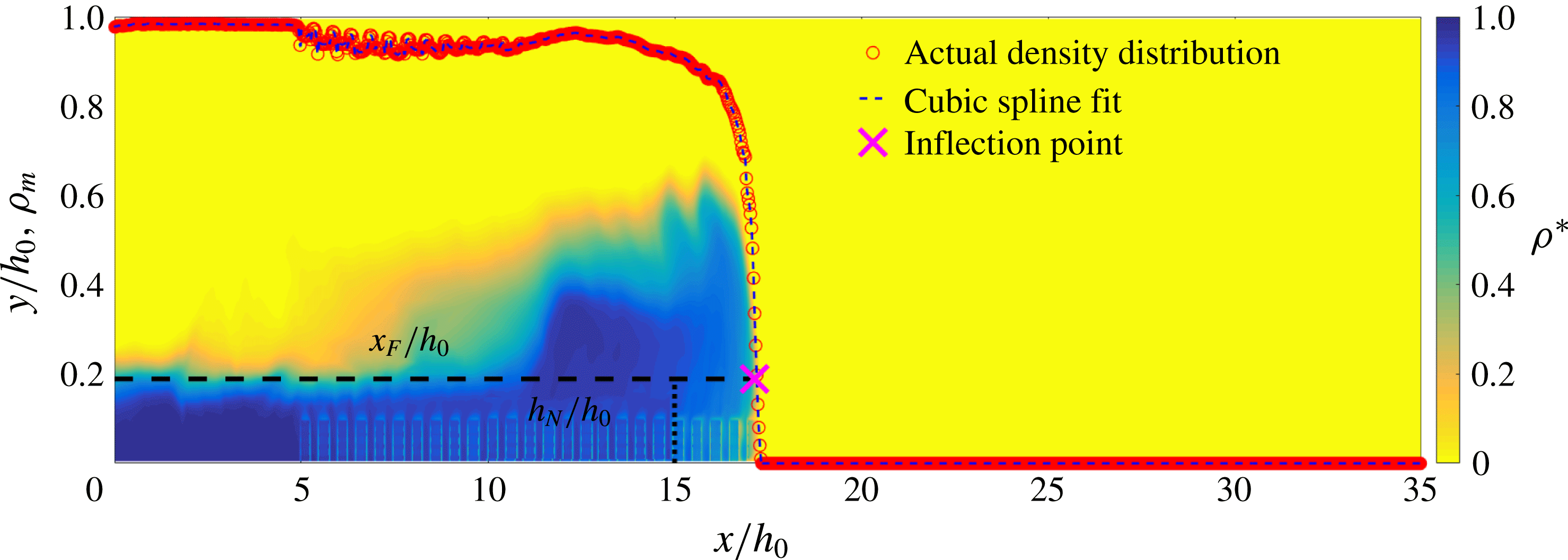
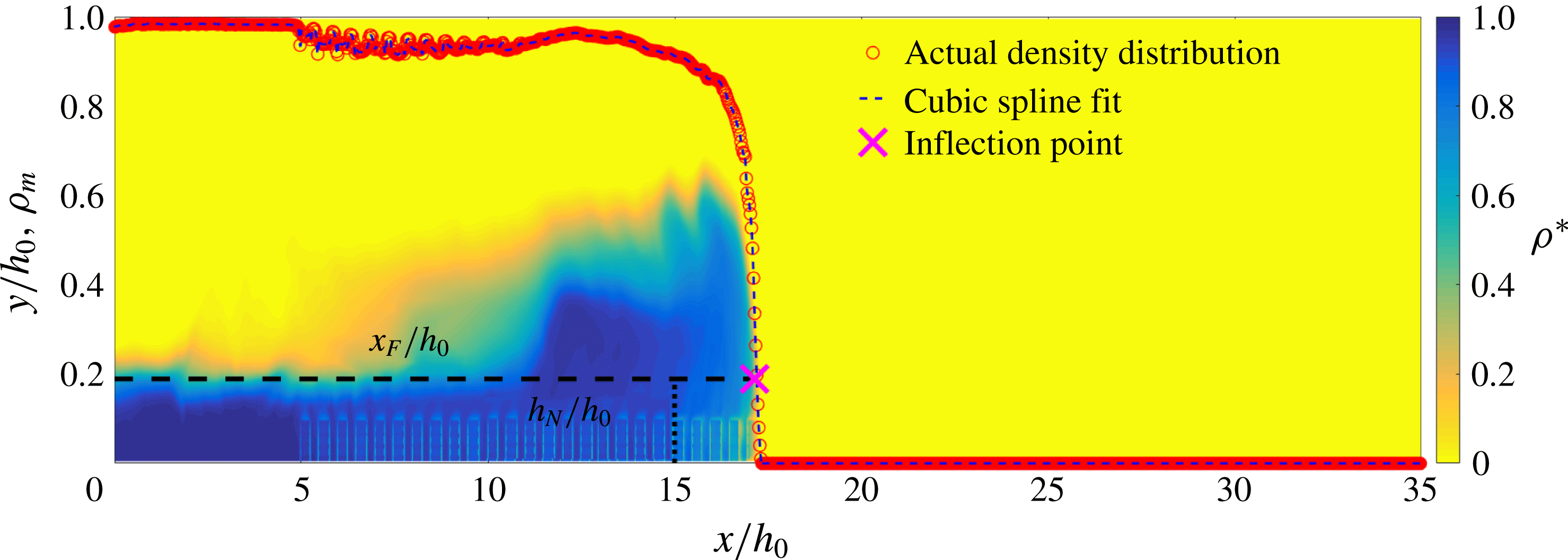
). From Benjamin’s (Reference Benjamin1968) theory, the curvature of the current switches from being negative near the nose to being positive above the nose; hence the inflection point of the maximum density (which always occurs closer to the lower wall) is an unambiguous way of obtaining the front location. The main advantage of this method is that there is no need to specify a density threshold value to identify the front location. We fit a cubic spline through the data and obtain an inflection point of the fitted function. Figure 2 shows an illustration of
 $\unicode[STIX]{x1D70C}_{m}$
versus
 $x$
plotted at
 $t=50$
s after the release of the gate. The cross sign marks the inflection point. Also shown in figure 2 is the 2D field of spanwise-averaged density at this corresponding time. The method captures the foremost point of the density current. The front speed (
 $u_{f}$
) is defined as the rate of change of
 $x_{f}$
, which has been calculated using (2.13).
The spanwise-averaged non-dimensional density field,
 $\unicode[STIX]{x1D70C}^{\ast }=(\unicode[STIX]{x1D70C}_{xy}-\unicode[STIX]{x1D70C}_{L})/(\unicode[STIX]{x1D70C}_{H}-\unicode[STIX]{x1D70C}_{L})$
for current advancing over uniform cubes. The subscript
 $xy$
refer to the 2D spatial location. Subscripts
 $H$
and
 $L$
identify the heavy and ambient fluids, respectively. Superimposed is the maximum density
 $(\unicode[STIX]{x1D70C}_{m})$
at each streamwise location at
 $t=50$
s (
 $\unicode[STIX]{x1D70C}_{m}=\max _{y}[\unicode[STIX]{x1D70C}^{\ast }(x,y,t)]$
).
2.4.2 Methodology for calculation of head height
In the potential energy method, the instantaneous depth of the current, which is the interface between the current and the ambient fluid, is defined as
 $$\begin{eqnarray}h(x,t)=2\frac{\displaystyle \int _{0}^{h_{0}}[\unicode[STIX]{x1D70C}(x,y,t)-\unicode[STIX]{x1D70C}_{L}]y\,\text{d}y}{\displaystyle \int _{0}^{h_{0}}[\unicode[STIX]{x1D70C}(x,y,t)-\unicode[STIX]{x1D70C}_{L}]\,\text{d}y},\end{eqnarray}$$
where
 $\unicode[STIX]{x1D70C}_{L}$
is the density of the ambient fluid. The first maximum from the leading edge of
 $h(x,t)$
is defined as the height of the head,
 $h_{H}$
,
 $$\begin{eqnarray}h_{H}=h(x^{\ast },t),\quad \text{where }x^{\ast }=\max \left\{x:\left(\frac{\text{d}h_{f}}{\text{d}x^{\ast }}\right)_{x=x^{\ast }}=0\right\}.\end{eqnarray}$$
3 Results
Six lock-exchange release experiments were performed for the cases shown in table 1. The simulations were conducted in a channel of length
 $L=4$
m and height
 $h_{0}=0.1$
m with a span
 $b=0.25$
m. The same initial conditions were used for all cases, with an initial reduced gravity of
 $g_{0}^{\prime }=0.05$
. The driving force, or equivalent pressure gradient, was the initial buoyancy in the lock,
 $B_{0}=g_{0}^{\prime }Lh_{0}b$
. Case 1 corresponds to a density current over smooth walls, and cases 2–6 correspond to density currents over rough walls. We begin our analysis by examining the front conditions.
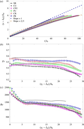
(a) Front location
 $x_{f}$
scaled with lock length versus non-dimensional time. See table 1 for details of the initials listed in the key. Also shown are the lines with constant slope of 1 and
 $2/3$
. (b) Froude number
 $Fr=u_{f}/(\sqrt{g_{0}^{\prime }h_{H}})$
versus non-dimensional front location. Symbols as in panel (a). (c) Reynolds number
 $Re=(u_{f}h_{H})/\unicode[STIX]{x1D708}$
versus non-dimensional front location. Symbols as in panel (a).

3.1 Front regimes
The front position scales with the lock length
 $(x_{f}-L_{0})/L_{0}$
versus non-dimensional time
 $t/t_{0}$
, where
 $t_{0}=h_{0}/\sqrt{g_{0}^{\prime }h_{0}}$
, as shown in figure 3(a). The front over the smooth wall with no roughness moves with a constant velocity, and hence the slope in the
 $x{-}t$
plot is unity, indicating that the current is in the slumping regime. The experimental results of Huppert & Simpson (Reference Huppert and Simpson1980) have clearly demonstrated that lock-exchange release density currents go through different well-defined regimes: slumping regime, in which buoyancy is constant, followed by an inertial regime, where the buoyancy forces are balanced by the inertial forces, resulting in
 $x_{f}\propto t^{2/3}$
. For the present case, the current over the smooth wall is in the slumping regime until the end of the simulation. Differences in the slopes and regimes are evident for the rough-wall cases. Two distinct regimes are evident for the rough-wall cases. In the initial regime, the slope of the trajectory in the
 $x{-}t$
plane varies with roughness and it is not constant in this regime but is within the following range: it is 0.92–0.99 for uniform cubes; 0.92–0.97 for the combination of uniform cubes and pyramids; 0.94–0.97 for uniform pyramids; 0.9–0.98 for the random cubes; and 0.93–0.99 for the random pyramids. As the slope is nearly 1, this regime can be well approximated as the slumping regime. It should be noted that, during the slumping regime over the rough wall, the presence of the spatial inhomogeneity in the vicinity of the roughness causes the large-amplitude temporal variation in the front velocity, resulting in varying slope within this regime. Hence, the variation of the slope is much higher for the random roughness cases compared to uniform roughness case. All the rough-wall cases show a transition from the slumping regime, where the slope changes suddenly, and current begins to slow down. The slope in this regime varies from 0.65 to 0.7, depending on the roughness type. At this time the current has entered the inertial regime. The analytic model of Tanino, Nepf & Kulis (Reference Tanino, Nepf and Kulis2005) predicts a slope of 0.67, where
 $x_{f}\propto t^{0.67}$
when the current is in the inertial regime. The slope obtained from the numerics is a close match to that predicted by theory. These results serve as a robust validation and confirm the presence of well-defined regimes for the density currents. They are consistent with the existence of the regimes from the theoretical study of Fay (Reference Fay1969) and substantiated by experiments (Fannelop & Waldman Reference Fannelop and Waldman1971; Hoult Reference Hoult1972).
3.2 Characteristic non-dimensional measures of the density currents
The non-dimensional numbers that characterize the state of density currents are the Froude number
 $(Fr)$
and the Reynolds number
 $(Re)$
. The Froude number reflects the transition of the potential energy available in the form of a heavy fluid into the kinetic energy of the propagating current, and it is defined as
 $Fr=u_{f}/\sqrt{g_{0}^{\prime }h_{H}}$
, where
 $u_{f}$
is the front velocity and initial reduced gravity is
 $g_{0}^{\prime }=g(\unicode[STIX]{x1D70C}_{H}-\unicode[STIX]{x1D70C}_{L})/\unicode[STIX]{x1D70C}_{L}$
(
 $\unicode[STIX]{x1D70C}_{H}$
represents density of the undiluted heavy fluid and
 $\unicode[STIX]{x1D70C}_{L}$
represents density of the ambient fluid). The Reynolds number is defined as
 $Re=u_{f}h_{H}/\unicode[STIX]{x1D708}$
. It should be noted that
 $Re$
is based on the local front velocity and the maximum depth of the current in the head region. Figure 3(b) shows the Froude number
 $Fr$
versus non-dimensional front location; the front over the smooth wall moves with a constant velocity of
 $Fr=0.56$
in the slumping regime. Roughness slows down the front due to enhanced drag, and
 $Fr$
decreases with roughness, with lowest value for uniform cubes, followed by uniform cubes and pyramids, uniform pyramids, random cubes and finally random pyramids. From this trend,
 $Fr$
decreases with increasing spanwise solidity
 $\unicode[STIX]{x1D6E4}_{1}$
. This is reasonable as the drag encountered by the front (leading edge of the current) depends on the ratio of the blockage due to roughness with respect to the cross-sectional area at that location. Hence, it is expected that
 $Fr$
shows a dependence on the spanwise solidity and this is consistent with theory. In the slumping regime, the mean
 $Fr$
varies from 0.42 to 0.52 for roughness cases. This result is consistent with the experiments of Keulegan (Reference Keulegan1958) and Barr (Reference Barr1963). Figure 3(c) shows the
 $Re$
versus non-dimensional front location. Here,
 $Re$
represents the local state of the current, as it is based on local velocity and length scales. As expected, the rough-wall cases have lower values of
 $Re$
than the smooth-wall example. However, it is interesting that for all the roughness cases the variation of
 $Re$
is in the range of 1290–1420 in the slumping regime, whereas deviation starts to appear towards the beginning of the inertial regime. We will explore this further when we discuss the mixing mechanisms.
Overall, it is clear that the current over the smooth wall is in the slumping regime throughout the simulation. The presence of roughness alters the behaviour of the front. As the solidity of roughness increases, the front travels with slower velocity in the slumping regime, and it transitions to the inertial regime much faster due to enhanced drag. When the front passes over the roughness elements, the spatial inhomogeneity in the vicinity of roughness causes high temporal variations in the data. Similar trends have been observed by Tokyay et al. (Reference Tokyay, Constantinescu and Meiburg2011) for 2D ribs; they noted that, as the front passed the crest and then the valley of the roughness, there was an increase in the potential energy and loss in kinetic energy at the crest, followed by a decrease in potential energy at the valley, and thus the front encountered sudden deceleration and acceleration as it passed through each roughness element. This results in large temporal variations in the front velocity.
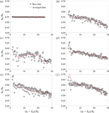
Variation in head height of advancing current: (a) smooth bed (SB), (b) pyramids with random height (PR), (c) cubes with random height (CR), (d) pyramids with uniform height (PU), (e) cubes and pyramids with uniform height (CPU), and (f) cubes with uniform height (CU).

3.3 Investigation of roughness metrics on current depth and head height
The depth of the instantaneous head location calculated using (2.15) is referred to as the head height. The variation of the head height as the front advances forwards is shown in figure 4. The importance of head height is that the higher the depth of the current, the higher the amount of volume of entrained fluid, and thus the greater the enhanced mixing in the current. During the slumping regime, the mean head height of the current over the smooth wall averages to
 $0.55h_{0}$
. The head height is greater for uniform cubes with mean values of
 $0.6h_{0}$
. The front, as it encounters the roughness peak, deflects upwards, and consequently the depth of the current increases, thus entraining more ambient fluid into the current. During the inertial regime, the mean height drops to
 $0.5h_{0}$
. Owing to the presence of pyramids, in both the uniform pyramids and the combination cases, irregularity in the depth of the head is evident. For the current over random cubes, a greater variation is clear, and the mean depth varies between
 $0.5h_{0}$
and
 $0.55h_{0}$
in the slumping regime; it drops to
 $0.48h_{0}$
in the inertial regime. Similar differences are observed between the current over pyramids of uniform height versus random height, where the mean
 $h_{H}$
is
 $0.55h_{0}$
during the slumping regime, and it drops to
 $0.5h_{0}$
in the inertial regime for pyramids of uniform height, whereas the significant variation in
 $h_{H}$
with the mean varies from
 $0.55h_{0}$
in the slumping regime to
 $0.45h_{0}$
in the inertial regime for pyramids of random height. It is clear that mean head height scales with volume fraction, as the uniform cubes with the highest volume fraction have more fluid volume in the head compared to the random pyramids with the lowest volume fraction, which have the least fluid volume in the head. Overall, the current over a rough wall entrains more ambient fluid compared to the smooth wall. Volume fraction, which is the volume occupied by the roughness elements in relation to the total volume of the channel, is an important metric that indicates roughness in the domain, and thus the greater the roughness, the higher the entrainment. The analysis has revealed that the volume fraction and solidity together dictate the differences in the flow characteristics due to surface roughness.
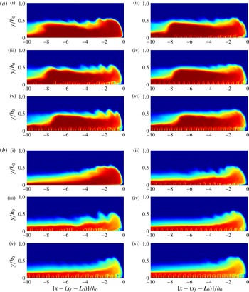
Evolution of the spanwise-averaged density field in a frame-invariant distribution with origin placed at the nose: (a) time = 40 s, (b) time = 80 s. The roman numerals represent (i) smooth bed (SB), (ii) pyramids with random height (PR), (iii) cubes with random height (CR), (iv) pyramids with uniform height (PU), (v) cubes and pyramids with uniform height (CPU), and (vi) cubes with uniform height (CU). Blue color represents density of the ambient fluid and red represents the undiluted lock fluid. The intermittent color distributions identify the dilution occuring on account of mixing.

3.4 Flow characteristics
In this section, we investigate the flow structures and the modifications of the flow physics due to the presence of roughness. The time evolution of the spanwise-averaged density fields at two different times corresponding to
 $t=40~\text{s}$
and
 $t=80~\text{s}$
is shown in figure 5. At each of the times, the difference between the six cases is compared. For the smooth-wall case, the two time instants correspond to the slumping regime, and a well-defined head is one of the dominant features of the flow, which remains undiluted throughout the slumping regime (i.e. for the entire simulation). At the leading edge of the current, the nose is slightly elevated above the ground. The 2D, shear-driven, KH instabilities form at the interface of the current and the ambient fluid above it. As the current advances forwards, the distinct region of relatively undiluted head and thinning tail region are evident. At both these time instants in the slumping regime, the current has a nearly constant head height. On comparing the rough-wall cases with the smooth-wall case, a distinct head region near the leading edge of the current similar to the smooth-wall case is present. During the early stages of the slumping regime, at
 $t=40~\text{s}$
, the dilution of the current near the nose (leading edge) is evident, which increases with increasing roughness. At a later time, i.e.
 $t=80~\text{s}$
, the head region is diluted for all the roughness cases, which is distinctly different from the smooth-wall case. Similar to the smooth-wall case, the tail region is relatively undiluted for the rough-wall case. However, the depth of the tail is higher due to the presence of roughness. The increase in roughness also results in faster dilution. Owing to the presence of roughness, the nose is elevated compared to the smooth wall. For the smooth-wall case, from the studies of Samasiri & Woods (Reference Samasiri and Woods2015) and Bhaganagar (Reference Bhaganagar2017), the head region is relatively undiluted as the constant mixing from the ambient fluid is compensated by the high-momentum lock fluid that enters the head and maintains a nearly constant buoyancy till the end of the slumping phase. However, surface roughness causes higher wall shear, resulting in a slowing down of the high-speed lock fluid, and hence resulting in faster dilution and mixing during the slumping regime. Overall, it is clear that, with identical initial conditions and for the same elapsed time, the head region is much diluted for rough cases compared to the smooth wall. The density fields clearly indicate increased mixing in the head region with increasing roughness, and more mixing occurs near the front end of the current.
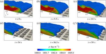
For the roughness comprising cubes of random elevations (CR), the iso-volumes of the density field (plotted up to 10 % threshold) are illustrated at selected time steps.

3.4.1 Flow structures
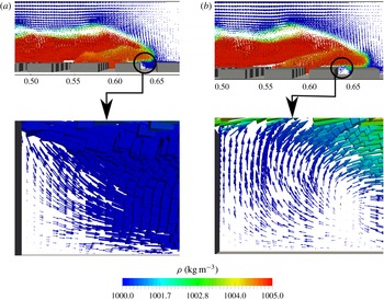
To understand the effect of roughness in altering the flow characteristics of the current, we now focus on the one case of random cubes. Figure 6(a–c) and (d–f) show the front advancing over cubes of random elevations in accelerating and slumping phases, respectively. The 2D KH instabilities develop early on during the acceleration regime and lead to the formation of the 3D characteristic lobe–cleft instabilities. As the front evolves, the lobe–cleft instabilities have a distinct signature of the underlying roughness elements. Furthermore, during the accelerating regime, the head region of the current forms, and the shape of the head also has a signature of the underlying roughness features. During this regime, the current is nearly filled with heavy fluid. There are 78 rows of roughness elements in the domain, between
 $7.2h_{0}\leqslant x_{f}\leqslant 8h_{0}$
; the front is crossing over the 14th row of roughness. In this row, the roughness elements have a height of up to
 $0.067h_{0}$
, as the front approaches them; because of the abrupt change in flow direction, portions of the head jump vertically up to the height of
 $0.4h_{0}$
and subsequently attach to the upper roughness surface. Owing to this impact, the front loses its momentum locally, yet convects over cubical obstructions by virtue of its potential energy. Crossing over the obstruction, the front splashes down towards the bottom bed at a distance of
 $d\approx RH_{n}$
(subscript
 $n$
denotes the
 $n$
th row of roughness elements whose height is
 $RH$
) downstream. Pockets of ambient fluid get trapped in the current in the valley region. Similar observations have been made by Tokyay et al. (Reference Tokyay, Constantinescu and Meiburg2011). The trapped ambient fluid gains momentum and the shear results in an additional local circulation, thus pushing these pockets into the heavy fluid propagating above them (figure 6
c). The heavy fluid flowing between roughness features acts as a catalyst in this mixing. However, this behaviour is localized, and exhibits strong coupling to the availability and height of roughness features, and the potential energy of the head. Furthermore, the impact between the front and the roughness features generates turbulent eddies, which in turn accelerate mixing in the head.
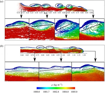
Front view of velocity fields during the (a) acceleration and (b) slumping phases for the current advancing over cubes of random height (CR). The colour distribution is in accordance with the density distribution whereas the arrows mark the direction of the velocity vector field. The horizontal scale signifies the dimensional distance in metres from the back (slip) wall of the channel.

Nose is crossing over a row of bottom roughnesses comprising cubes of uniform elevation (CU). Panels (a) and (b) are captured on a 2D plane at
 $t=4.5~\text{s}$
and
 $5.5~\text{s}$
, respectively. The colour distribution is in accordance with the density whereas the arrows mark the direction of the velocity vectors. The illustration clearly depicts circulation in the wake of a roughness feature and the consequent dilution. The horizontal scale signifies the dimensional distance in metres from the back (slip) wall of the channel.

Substantial mixing also takes place via KH rollers at the shear interface, as seen in figure 7(a,b), illustrated by the velocity vectors plotted on a plane positioned midspan, during the two instants of the slumping regime. The colour distribution is set proportional to the density concentration to convey the idea of ambient fluid entering the current. Here, KH rollers can be seen creating a strong circulation, resulting in the ambient fluid being entrained into the current. During the initial phases (figure 7
a), distinct regions of circulation are located at
 $x=2.5h_{0}$
,
 $4h_{0}$
,
 $5.6h_{0}$
and
 $6.75h_{0}$
. As the current advances and within the slumping regime, the presence of additional shear stretches the circular mixing zones into elliptical recirculating zones. In figure 7(b), these recirculating regions are at
 $x=7.4h_{0}$
,
 $8.4h_{0}$
and
 $11h_{0}$
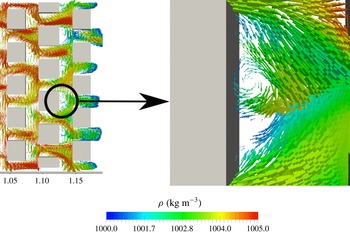
. Furthermore, as seen in figure 8, there is a recirculating region formed near the leading edge of the current that displaces the ambient fluid, and a fraction of the ambient fluid enters the current and the remainder is pushed in the opposite direction from the front. These findings are consistent with those of Kneller et al. (Reference Kneller, Bennett and McCaffrey1999), who used laser Doppler anemometry to reveal, for a smooth wall, a vortex near the head with strong circulation within the head region. In addition to the mixing that happens at the current interface, it is clearly seen in figure 8 that, as the current travels between the two successive roughness elements, the ambient fluid trapped between the roughness elements gains momentum, and the shear results in a local recirculation region between the roughness elements. The additional vorticity that is generated causes the ambient fluid to mix with the mixed fluid, further diluting the current. This additional dilution is local and occurs between the roughness elements. This can be further understood by examining the top view in figure 9. It shows the velocity vectors plotted on a plane lying halfway between the roughness height for the domain containing cubes of uniform height. The vectors are coloured according to density distribution. As the current passes over the roughness elements, the portion over the roughness peaks slows down, and that flowing between the valley regions accelerates. At
 $t=50~\text{s}$
, the heavy fluid traverses over the roughness peaks, resulting in the formation of a shear layer that disturbs the ambient fluid in the valley regions of the roughness, which mixes with the current and the mixed fluid that passes through the valleys.
The additional mixing occurs due to roughness elements that act as mixing rollers that mix the trapped ambient fluid under the frontal region of the current with the mixed fluid within the current, resulting in additional dilution. Now the question that needs to be investigated is this: What metric dictates the amount of mixing and dilution that takes place due to the presence of roughness? Roughness elements are more efficient generators of skin friction than their smooth counterparts, and hence the rough wall has greater shear, and consequently greater
 $Re_{\unicode[STIX]{x1D70F}}$
compared to a smooth wall (e.g. Bhaganagar et al.
Reference Bhaganagar, Kim and Coleman2004; Jimenez Reference Jimenez2004; Orlandi & Leonardi Reference Orlandi and Leonardi2004). The shear layer developed in the roughness region is analysed next.
Flow field plotted on a plane normal to the elevation as the nose crosses a row of bottom roughnesses comprising cubes of uniform elevation (CU). The arrows mark the direction of the velocity vectors whereas the colour distribution is in accordance with the local density distribution. The horizontal scale signifies the dimensional distance in metres from the back (slip) wall of the channel.

3.5 Shear stress
Contours of shear distribution calculated from the spanwise-averaged streamwise velocity field plotted at
 $t=67.5~\text{s}$
: (a) smooth bed (SB), (b) pyramids with random height (PR), (c) cubes with random height (CR), (d) pyramids with uniform height (PU), (e) cubes and pyramids with uniform height (CPU), and (f) cubes with uniform height (CU).

(a) Ratio of the shear at the interface to the shear at the rough wall versus front location. (b) Maximum shear recorded at the interface. (c) Friction Reynolds number. See figure 3 for key.

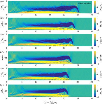
Figure 10 shows the spanwise-averaged shear plotted in the
 $x{-}y$
plane for all the cases compared at
 $t\approx 67.5~\text{s}$
. Regions of high shear are seen at the interface near the head, and near the lower wall. The KH rollers cause the large velocity gradients at the interface in the head region. Additionally, high wall shear stress is in region
 $x=20{-}25$
, and this corresponds to
 $x/L_{0}=1$
, which is one lock length. At the lower wall, due to the no-slip condition, the shear layer emanates from the wall. Bhaganagar (Reference Bhaganagar2017) observed that entrainment occurs within one lock length from the nose, and that the region is designated as the active head region of the current. For all the rough cases (figure 10
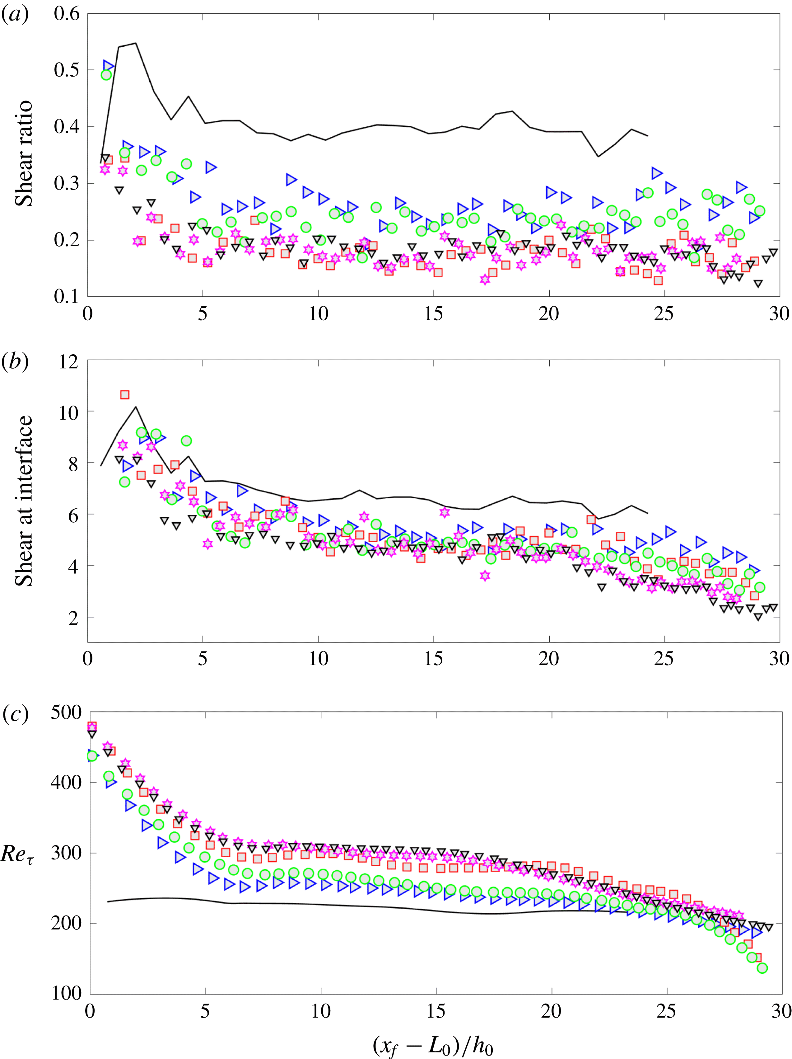
b–f), similar to the smooth wall, high shear at the interface is mainly in the head region of the current, and this is due to the KH rollers. In addition, large wall shear exists on roughness peaks, and thus exhibits a signature of roughness. An important difference that exists between the smooth wall and the rough wall is the following. For the smooth wall, strong shear layers exist at the interface of the current and ambient fluid as well as in the neighbourhood of the bottom wall. The latter is a thin layer, and no interaction takes place between the two shear layers. In the case of the rough wall, a similar shear layer at the interface of the current and ambient fluid exists; however, the shear layer at the rough (bottom) wall is stronger and deeper, and has a signature of the underlying roughness. To get clarity on the strength of the shear layer at the interface versus the lower rough wall, we plot maximum shear at the interface versus front location in figure 11(b), and the friction Reynolds number,
 $Re_{\unicode[STIX]{x1D70F}}$
, obtained from wall shear stress, versus front location in figure 11(c), respectively. The rough wall has a higher
 $Re_{\unicode[STIX]{x1D70F}}$
compared to the smooth wall, as expected, and differences between the roughness geometries exist. The values of
 $Re_{\unicode[STIX]{x1D70F}}$
range between 245 and 306 (in the slumping phase). However, the maximum values occur right after the lock release, and the value is as high as 500. As the current advances forwards, wall shear is nearly constant with
 $Re_{\unicode[STIX]{x1D70F}}$
of 220 throughout the slumping regime for the smooth-wall case. During the slumping regime, the uniform cubes have the highest
 $Re_{\unicode[STIX]{x1D70F}}$
of 306, followed by cubes and pyramids of uniform height with
 $Re_{\unicode[STIX]{x1D70F}}$
of 298, cubes of random height with
 $Re_{\unicode[STIX]{x1D70F}}$
of 285, pyramids of uniform height with
 $Re_{\unicode[STIX]{x1D70F}}$
of 258, and finally, pyramids of random heights with
 $Re_{\unicode[STIX]{x1D70F}}$
of 245. Therefore,
 $Re_{\unicode[STIX]{x1D70F}}$
is a representation of the dynamics of roughness, and in the subsequent analysis, presented in the next section, it is demonstrated that
 $Re_{\unicode[STIX]{x1D70F}}$
is the key metric that represents the influence of roughness on enhanced mixing in the current. Finally, to get clarity on the relative magnitude of the shear layer at the interface versus the lower wall, the ratio of maximum shear at the interface to that of the bottom bed is plotted in figure 11(a). After the initial transience, the maximum shear at the interface of the current and ambient fluid is around 0.4, whereas for the rough wall this shear is lower (in the range of 0.15–0.3, depending on the roughness). The fraction of the shear due to KH rollers, with respect to wall shear, is smaller for the rough wall compared to the smooth wall. Scaled by the wall roughness, the KH rollers are weaker due to the presence of roughness.
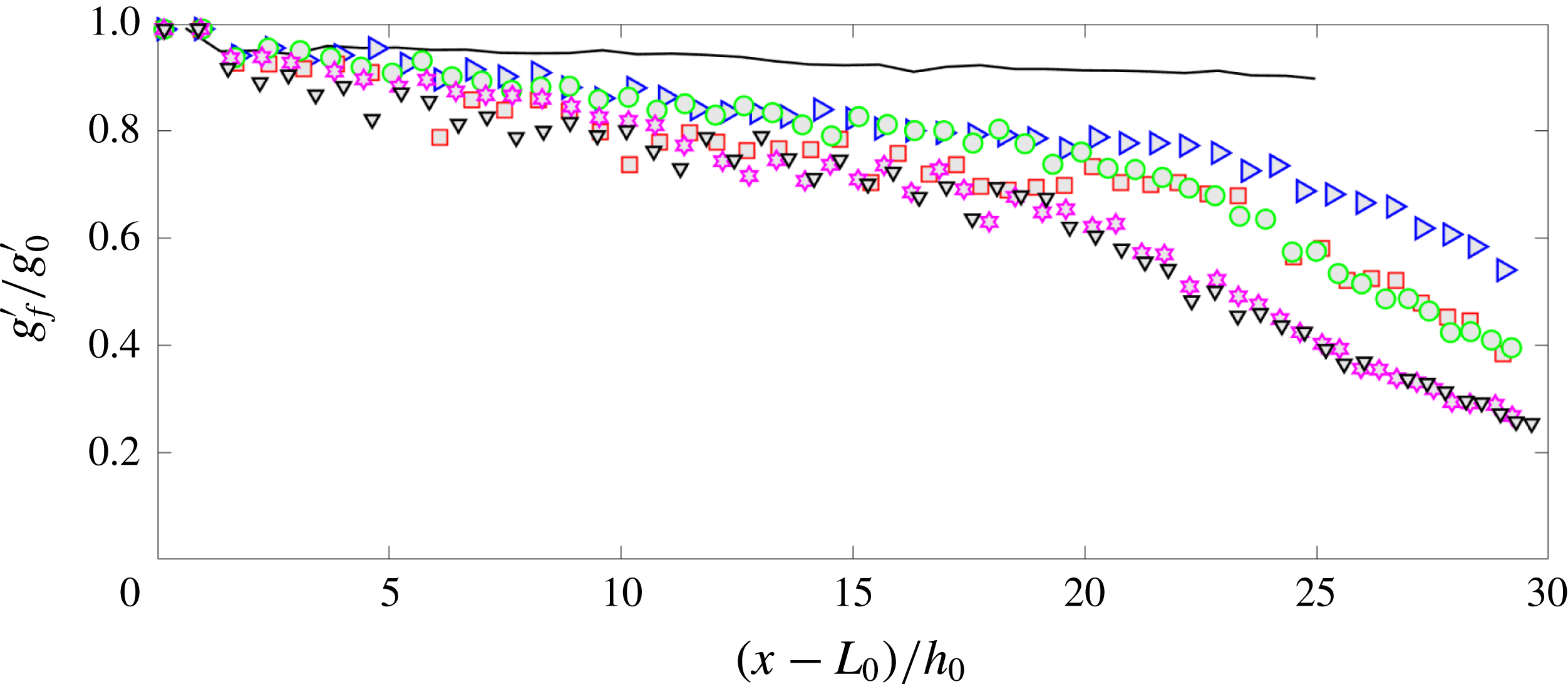
Local reduced gravity
 $g_{f}^{\prime }$
scaled with the initial reduced gravity
 $g_{0}^{\prime }$
in the lock versus the front location. See figure 3 for key.

3.6 Mixing and entrainment
Next, we quantify the mixing process based on the reduced gravity at the front (
 $g_{f}^{\prime }$
), defined as
 $g_{f}^{\prime }=\widetilde{g_{e}^{\prime }}\widetilde{h}_{H}/h_{H}$
, where
 $\widetilde{g_{e}^{\prime }}\widetilde{h}_{H}=g\int _{0}^{h_{0}}[(\unicode[STIX]{x1D70C}(x^{\ast },y,t)-\unicode[STIX]{x1D70C}_{L})/\unicode[STIX]{x1D70C}_{L}]\,\text{d}y$
. In figure 12,
 $g_{f}^{\prime }$
scaled by the initial reduced gravity (
 $g_{0}^{\prime }$
), defined as
 $g_{0}^{\prime }=g(\unicode[STIX]{x1D70C}_{H}-\unicode[STIX]{x1D70C}_{L}/\unicode[STIX]{x1D70C}_{L})$
, is plotted as a function of
 $x_{f}$
. For the smooth wall, the current is entirely in the slumping regime, and
 $g_{f}$
is nearly constant at a fraction of 0.9–1.0 of the original lock fluid, which implies that the local buoyancy in the head does not change when the current is in the slumping regime. In the roughness cases, a notable difference is that more mixing is evident. Two regimes are clearly evident from figure 12 for the rough-wall cases. Unlike the smooth wall, the rough wall shows more variation within the slumping regime, as
 $g_{f}^{\prime }$
varies between 0.8 and 0.9, which indicates that mixing due to roughness starts early on in the slumping regime, causing dilution and thus reduction in buoyancy. A consistent trend is observed in the front trajectory, as seen in figure 3(a), where, during the slumping regime, there is a loss of buoyancy and the slope of the front trajectory varies between 0.92 and 0.99. In the next regime, high dilution and mixing is evident for the rough-wall case. In addition, significant differences between the rough-wall cases are evident in the inertial regime. The greater the roughness, the faster is the dilution at the front. In the inertial regime, for uniform cubes,
 $g_{f}^{\prime }$
drops from 0.8 to 0.1 by the time the front reaches
 $x=30h_{0}$
from the gate. A similar trend is also evident for the combination of cubes and pyramids of uniform height. For the same distance, the dilution for random pyramids is from 0.9 to 0.5. In the other cases the dilutions are between these values, from 0.8 to 0.3 for random cubes, and from 0.9 to 0.4 for random pyramids. As a note, an alternative definition of bulk reduced gravity in the head has been used to evaluate the reduced gravity and no significant difference has been observed in the mixing, in either the slumping or inertial regimes, thus giving us confidence that the front is a representation of mixing in the head for rough walls as well.
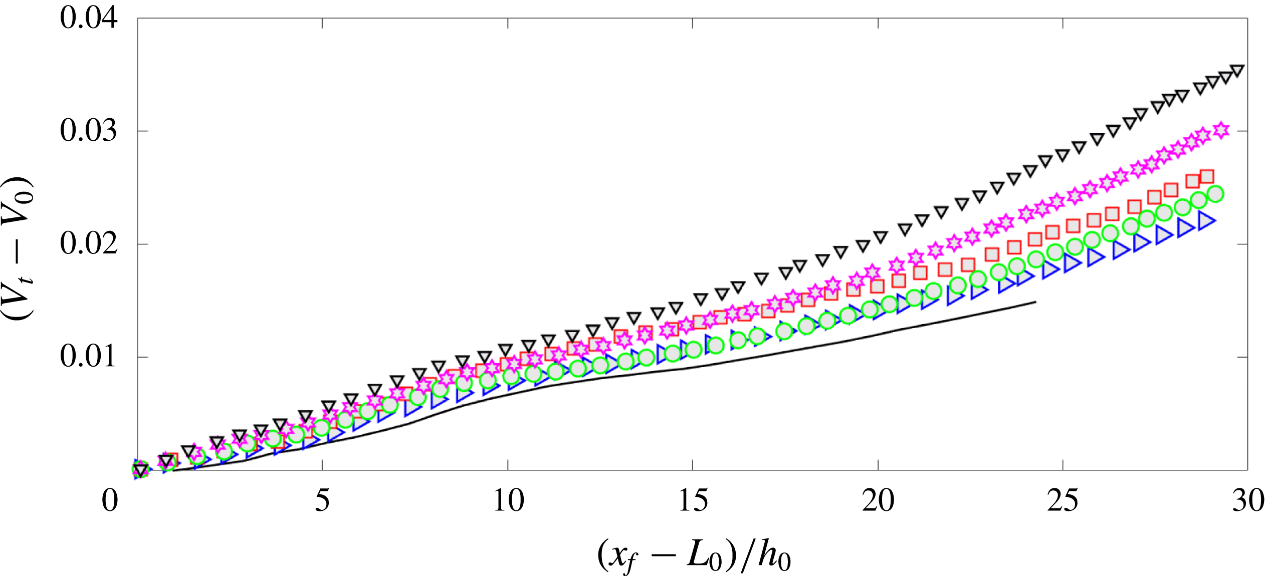
Change in volume of the current with respect to the initial lock volume plotted against the front location. See figure 3 for key.

The instantaneous entrainment parameter is the amount of ambient fluid that enters the current, and hence is defined as the increase in the volume of the fluid in the current from the initial lock volume in time
 $t$
scaled by the length of the current (distance between the nose and the tail or lock gate) and the velocity of the front (
 $u_{f}$
):
 $$\begin{eqnarray}E_{l}(t)=\frac{V(t)-V_{0}}{lu_{f}t}.\end{eqnarray}$$
Here,
 $V(t)$
is the volume of the dense fluid,
 $V_{0}$
is the volume of the initial lock fluid and
 $l$
is the length of the current. The volume of the current is defined as
 $V(t)=\int _{0}^{x_{f}}h(x,t)\,\text{d}x$
. Figure 13 shows
 $V(t)$
versus nose location
 $(x_{f})$
. For the smooth wall, after an initial acceleration period, the volume increases at a non-uniform rate. The volume occupied under the current is higher for rough walls, and this increases with increasing roughness. The greater the volume fraction of roughness, the greater the volume occupied by the mixed fluid in the current.
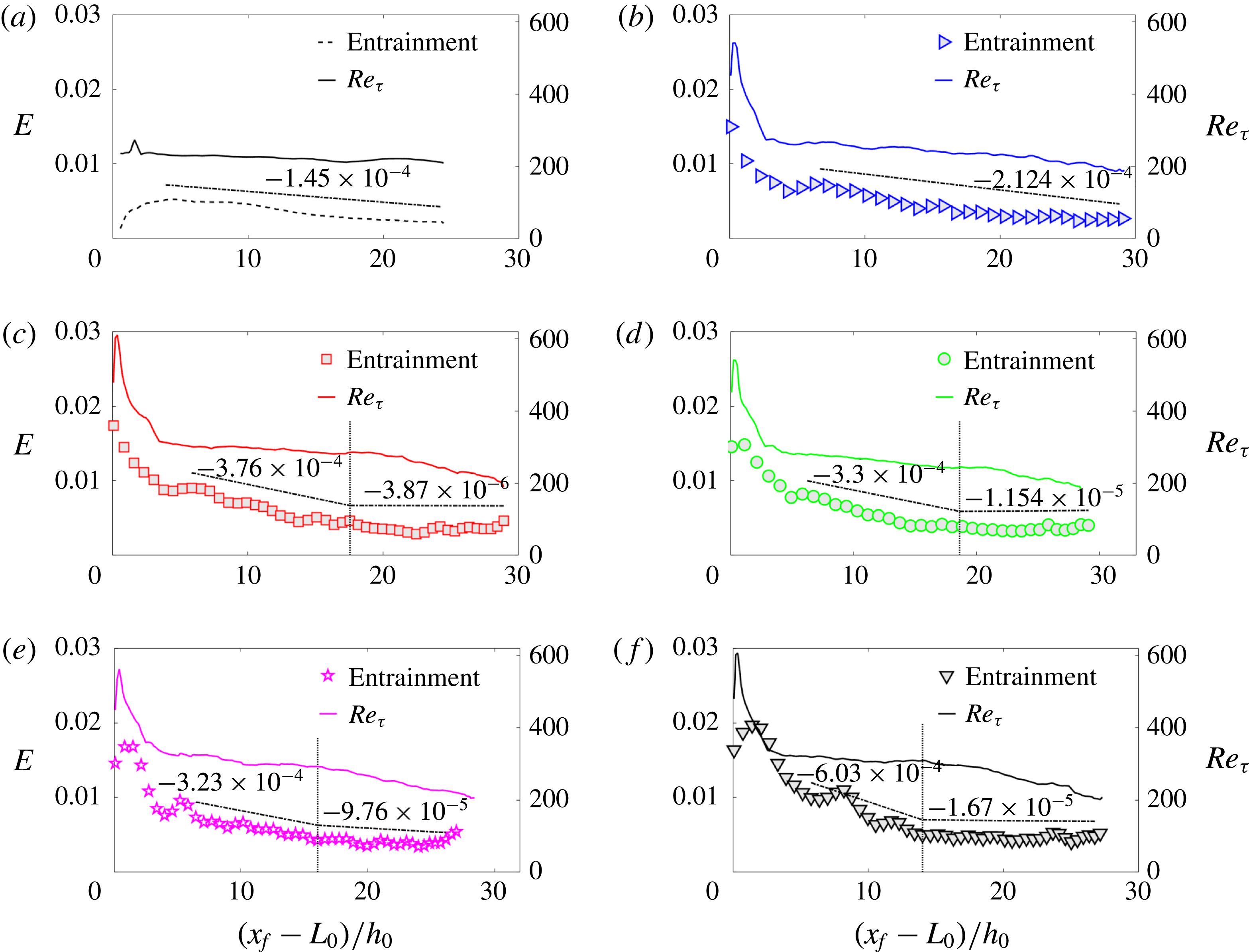
Figure 14 shows instantaneous entrainment coefficient
 $E$
on the primary
 $y$
-axis versus the front location for all the cases. The vertical lines represent the location where the front transitions from the slumping to the inertial regime. In figure 14,
 $Re_{\unicode[STIX]{x1D70F}}$
is plotted on the secondary
 $y$
-axis. Also shown is the slope of
 $E$
versus
 $x_{f}$
, which has been calculated separately in the slumping and inertial regimes. As the volume fraction increases, the slope of
 $E$
versus
 $x_{f}$
increases from
 $1.45\times 10^{-4}$
to
 $6.03\times 10^{-4}$
. By the end of the slumping regime,
 $E$
reaches a quasi-equilibrium value, as seen from the slope in the inertial regime, which is at least one order of magnitude less than that in the slumping regime. The observation for the rough-wall cases is that, with increasing volume fraction, entrainment during the beginning of the slumping regime is higher, the rate at which the entrainment drops (slope) is faster, and the final steady-state value reached at the end of the slumping regime is higher. As seen from
 $Re_{\unicode[STIX]{x1D70F}}$
(secondary
 $y$
-axis) versus
 $x_{f}$
in figure 14, during the slumping regime
 $Re_{\unicode[STIX]{x1D70F}}$
does not show significant variation, and it drops drastically during the inertial regime, as the drag due to roughness dominates the flow dynamics. The higher the volume fraction, the higher is the
 $E$
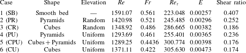
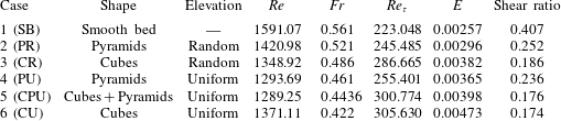
value during the slumping regime. This trend is clearly seen in table 2, where the averaged values of
 $E$
,
 $Re$
,
 $Fr$
and
 $Re_{\unicode[STIX]{x1D70F}}$
during the slumping regime are presented. A strong correlation exists between
 $E$
and
 $Re_{\unicode[STIX]{x1D70F}}$
.
Variation in entrainment coefficient and turbulent Reynolds number: (a) smooth bed (SB), (b) pyramids with random height (PR), (c) cubes with random height (CR), (d) pyramids with uniform height (PU), (e) cubes and pyramids with uniform height (CPU) and (f) cubes with uniform height (CU).

Averaged values of
 $Re$
,
 $Fr$
,
 $Re_{\unicode[STIX]{x1D70F}}$
,
 $E$
and shear ratio during the slumping regime.
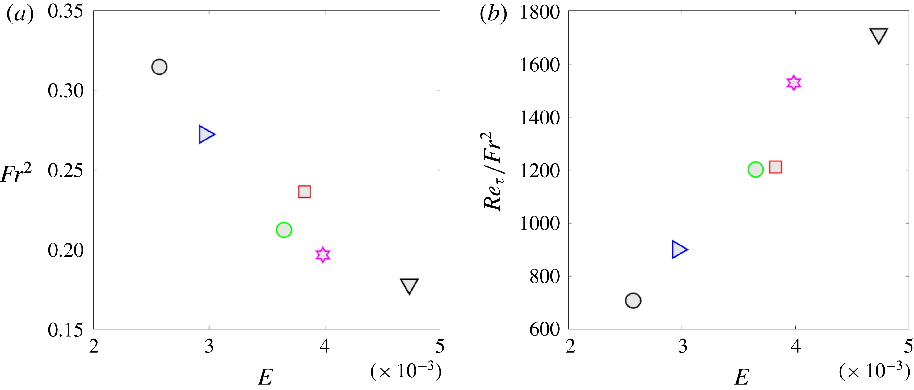
Though the focus of this study is to shed light on the unsteady nature of mixing in the density current, we calculate the mean values of
 $E$
averaged over the slumping regime and present them in figure 15(a,b). Here, the mean
 $E$
is plotted against the averaged value of
 $(Fr^{2})$
and
 $Re_{\unicode[STIX]{x1D70F}}/Fr^{2}$
, respectively. The average
 $Fr^{2}$
correlates with
 $E$
for some cases, but discrepancy in the correlation is seen. We have observed that
 $Fr$
correlated with the spanwise solidity, and that
 $E$
correlated with volume fraction; hence, the trend observed is expected, and
 $Fr$
is lower for random pyramids than for random cubes, but the entrainment coefficient for random cubes is higher than for random pyramids. A better correlation of
 $E$
with
 $Re_{\unicode[STIX]{x1D70F}}/Fr^{2}$
is seen in figure 15(b). It should be noted that the average
 $Re$
for all the roughness cases considered varies within a smaller range of 1290–1420 (see table 2). To understand the effect of
 $Re$
on this relation with
 $E$
, additional experiments, e.g. with different initial conditions, are needed. It is clear that for the low-Reynolds-number density currents with roughness elements within the current, in addition to
 $Fr$
, the entrainment coefficient also depends on
 $Re_{\unicode[STIX]{x1D70F}}$
.
Mean entrainment coefficient in the slumping phase plotted against (a) the square of the mean Froude number
 $(Fr^{2})$
and (b) the ratio of
 $Re_{\unicode[STIX]{x1D70F}}$
and
 $Fr^{2}$
. See figure 3 for key.

4 Conclusions
LES have been conducted to simulate 3D lock-exchange release density currents over smooth and rough surfaces. A highly accurate and novel penalization-based method has been developed to introduce complex geometry. The primary objective of this work is to establish a firm foundation for the effect of surface roughness on front characteristics and mixing in the current. Surface roughness adds significant complexity both to the flow dynamics and to the flow analysis. Study of rough walls is complicated due to the influence of various roughness parameters that the wall introduces into the flow physics. The distribution and shape of roughness elements are important indicators that influence the flow dynamics; hence the differences that exist between roughness elements with the same height versus those with irregular heights are important.
The near-wall region of the density current has a significant role in modifying the flow dynamics, and wall shear
 $(\unicode[STIX]{x1D70F}_{w})$
dictates the drag encountered by the current. Among the roughness metrics, the roughness density is the metric that influences
 $\unicode[STIX]{x1D70F}_{w}$
. In this study, the volume fraction and roughness solidity were varied by changing the shapes of cubes and pyramids (stepped cubes) with uniform height and random height distributions. The simulations were performed under the same conditions, including domain size, lock conditions (height and aspect ratios) and with the same initial reduced gravity and buoyancy.
Surface roughness has an important effect on density currents, and it significantly alters the front characteristics and mixing within the current. The potential-energy method developed by Anjum et al. (Reference Anjum, McElwaine and Caulfield2013) provides a consistent approach to obtain the current depth, as it is unambiguous, unlike the commonly used threshold method. We develop a consistent manner to estimate the interface height, front height (height of the head) and definitions of
 $Fr$
and
 $Re$
, which is suitable for rough surfaces. It is important for future studies on roughness to use consistent and accurate definitions that define the front. As per Benjamin’s (Reference Benjamin1968) theory, the curvature of the current switches from being negative to being positive near the nose, and hence the inflection point of the maximum density at each streamwise location
 $x$
defines the nose (
 $x_{f}$
) and the rate of the change of
 $x_{f}$
is the front velocity (
 $u_{f}$
).
Peters & Venart (Reference Peters and Venart2000) conducted experiments on density currents over 2D square cross-sectional elements and obtained constant slopes of
 $0.91\pm 0.04$
during the slumping regime, and
 $2/3$
in the inertial regime. It is important to note that the slumping regime does exist for the rough wall, where the current moves with nearly uniform velocity, but the slope of the front trajectory is not exactly unity, as in the smooth-wall case. The main difference is that the buoyancy is conserved during the slumping regime, whereas a low amount of mixing is present for rough-wall cases, as the shear layer near the roughness elements acts as an efficient mixing roller during the early stages of the slumping regime. For all the roughness cases considered, two distinct regimes are clearly evident. During the slumping regime, the mixing as obtained from the reduced gravity is between 0.8 and 1.0, indicating some loss of buoyancy in the slumping regime. This is followed by an inertial regime, with faster loss of buoyancy as the front advances.
Surface roughness slows down the density currents and
 $Fr$
decreases with increasing streamwise solidity (
 $\unicode[STIX]{x1D6E4}_{1}$
), as the front velocity depends on the ratio of roughness area blockage with respect to the cross-sectional area facing the front. A well-defined head is evident for currents over roughness in the slumping regime, and the shape of the head has a signature of the underlying roughness features. As the current travels between two successive roughness elements, the ambient fluid trapped between the roughness elements gains momentum, and the shear results in a local recirculation region between the roughness elements. The additional vorticity that is generated causes the ambient fluid to mix with the mixed fluid, further diluting the current. This additional dilution is local and occurs between the roughness elements. Increased surface roughness over which the density current flows leads to increased wall shear stress, mainly in the head region of the current. Density currents over roughness surfaces have higher deceleration and increased mixing.
Flow visualization has revealed that, during the early stages of slumping, the KH rollers are circular, but the shearing acting on the interface elongates these rollers during the later stages of slumping. This is different than for smooth walls (figures are not shown for smooth walls). The elongation causes the strength of KH rollers to weaken. The strength of the KH rollers has been evaluated from the shear at the interface (figure 11
b). The KH rollers are weaker for a rough wall compared to a smooth wall. It is interesting to note that the differences due to the near-wall influence of roughness does not influence the strength of KH instability, and hence the mean shear at the interface (averaged during the slumping regime) is nearly the same for all the roughness cases, suggesting that roughness reduces the strength of KH rollers compared to the smooth-wall case; however, the differences in roughness shape and distribution do not influence them significantly. It is very likely that the strength of the KH rollers is influenced by the initial conditions of the lock. The velocity vectors indicate that, as the current moves over the roughness peaks, the shear layer generated from the peaks is strong, and depends on the roughness, and it is comparable in strength to the KH shear layer. The behaviour is similar to that observed in constant-density flows over roughness, where the roughness causes the shear layer lift-up. The ambient and stationary fluid in the valleys gains momentum and the shear layer formed over the roughness propels the fluid vertically upwards, thus generating vorticity in this region, the consequence of which is additional mixing and dilution of the current. In principle, the entrainment occurs from two sources: the primary source of entrainment is at the interface, where the shear entrains the ambient fluid near the interface, which has been displaced by the current; and the secondary source is due to the shear layer lift-up (as seen in figure 10) resulting in roughness-induced vorticity that causes additional mixing. For the primary source of entrainment, the extent of mixing is mainly dictated by front conditions (namely,
 $Re$
). For the latter, the roughness-induced vorticity is mainly dictated by the amount of wall shear generated by the roughness. Hence, a measure of the wall shear stress dictates the latter source of entrainment.
The instantaneous entrainment coefficient, defined as the increase in the volume of the fluid in the current from the initial lock volume in time
 $t$
scaled by the length of the current (distance between the nose and the tail or lock gate) and the velocity of the front, revealed insightful information on the unsteady entrainment process. For the rough-wall cases with increasing volume fraction we have the following results: entrainment during the beginning of the slumping regime is higher; the rate at which the entrainment drops (slope of
 $E$
and
 $x_{f}$
) is faster; and the final steady-state value reached at the end of the slumping regime is higher. It is clear that entrainment begins during the early stages of the slumping regime, and the rate of entrainment is at least an order of magnitude higher during the slumping regime than in the inertial regime. Finally, as shown in table 2, where the averaged
 $E$
has been calculated during the slumping regime, it shows a trend with the averaged
 $Re_{\unicode[STIX]{x1D70F}}$
. It should be noted that, for the roughness cases selected in the study,
 $Re$
varies within a smaller range of 1290–1420.
The high-resolution LES simulations of Tokyay et al. (Reference Tokyay, Constantinescu and Meiburg2012) for 2D dunes and 2D ribs demonstrated that the spatial distribution of the friction velocity
 $u_{\unicode[STIX]{x1D70F}}$
can be correlated to entrainment. In this study, we demonstrate that
 $Re_{\unicode[STIX]{x1D70F}}$
based on
 $u_{\unicode[STIX]{x1D70F}}$
and the local height of the current
 $(h_{H})$
is an appropriate metric that quantifies the additional entrainment and mixing that results due to the roughness dynamics. The study provides further support to the theory posed by Fernandez & Imberger (Reference Fernandez and Imberger2006) that entrainment depends on the stress generated at the bottom, and obtained by the roughness and the current properties. The present study is novel and presents a framework for analysing entrainment of density currents over roughness. It is important to conduct future experimental and numerical studies for a much larger range of roughness volume fraction and solidity under different
 $Re$
conditions. This study is one of the first to conduct an analysis of the unsteady nature of the entrainment during the slumping and inertial regime over 3D roughness, and it clearly demonstrates an important need to study the entrainment process in time. These future studies will provide guidance to relate local entrainment to current properties (namely,
 $Re$
and
 $Fr$
) and roughness properties (
 $Re_{\unicode[STIX]{x1D70F}}$
).
Acknowledgements
Funding for this research was provided by the National Science Foundation, Division of Physical Oceanography grant no. OCE-1333033, and US Army Edgewood Chemical and Biological Center, MSRDC grant no. D01-W911SR-14-2-0001-0006. The authors acknowledge the Texas Advanced Computing Center (TACC) at the University of Texas at Austin (http://www.tacc.utexas.edu) for providing computational and visualization resources that have contributed to the research results reported within this paper.
Appendix A. Symbols and notation