1. Introduction
The fluctuating pressure field induced by a turbulent boundary layer (TBL) can generate significant noise and vibrations at the wall beneath it. This has the potential to adversely affect many systems given that TBLs are present in a variety of engineering applications. For example, TBL-induced wall-pressure fluctuations are a major source of noise and vibration in high-speed vehicles (Cockburn & Robertson Reference Cockburn and Robertson1974; Wilby Reference Wilby1996; Arguillat et al. Reference Arguillat, Ricot, Bailly and Robert2010), resulting in passenger discomfort (Mellert et al. Reference Mellert, Baumann, Freese and Weber2008) and the potential for structural excitation (Leehey Reference Leehey1988). These same wall-pressure fluctuations result in acoustic scattering at the trailing edges of wing profiles and other similar geometries (Ffowcs Williams & Hall Reference Ffowcs Williams and Hall1970; Brooks, Pope & Marcolini Reference Brooks, Pope and Marcolini1989), leading to additional noise generation. Improving our knowledge of these fluctuations will undoubtedly assist engineers in the design process, but is also critical to the development of turbulence models and flow control strategies. The latter are particularly reliant on knowledge of the wall-pressure fluctuations because flow control strategies generally demand wall-based sensing and actuation. There is therefore considerable motivation for the study of the wall-pressure fluctuations induced by a TBL.
An important feature of mid- to high-Reynolds number TBLs that has yet to be clearly linked to wall pressure is the presence of ‘very-large-scale motions’ (VLSMs) (Kim & Adrian Reference Kim and Adrian1999) or ‘superstructures’ (Hutchins & Marusic Reference Hutchins and Marusic2007a) in the logarithmic and wake layers of the flow. These motions are characterized as long, meandering regions of high and low streamwise velocity fluctuation with lengths greater than approximately three times the boundary layer thickness  $\delta$ (Balakumar & Adrian Reference Balakumar and Adrian2007). Their instantaneous widths and heights are mostly around
 $0.5\delta$ or less (Dennis & Nickels Reference Dennis and Nickels2011a), and they have been observed to extend beyond
 $20\delta$ in length (Hutchins & Marusic Reference Hutchins and Marusic2007a). Although the VLSMs are a recent discovery relative to the long history of TBL research, they have emerged as being critical to the dynamics of the flow. They carry a considerable amount of kinetic energy and Reynolds shear stress (Balakumar & Adrian Reference Balakumar and Adrian2007; Lee & Sung Reference Lee and Sung2011), are responsible for modulating the amplitude and frequency of near-wall fluid motions (Hutchins & Marusic Reference Hutchins and Marusic2007b; Mathis, Hutchins & Marusic Reference Mathis, Hutchins and Marusic2009; Ganapathisubramani et al. Reference Ganapathisubramani, Hutchins, Monty, Chung and Marusic2012), and are associated with extreme wall-shear events (Hutchins et al. Reference Hutchins, Monty, Ganapathisubramani, Ng and Marusic2011; Pan & Kwon Reference Pan and Kwon2018). There is evidence that large-scale motions (LSMs), which consist of the largest of a hierarchy of hairpin packets (Adrian Reference Adrian2007; Smits, McKeon & Marusic Reference Smits, McKeon and Marusic2011), concatenate or merge to form the VLSMs (Kim & Adrian Reference Kim and Adrian1999; Balakumar & Adrian Reference Balakumar and Adrian2007; Lee & Sung Reference Lee and Sung2011; Lee et al. Reference Lee, Lee, Choi and Sung2014). Consequently, both the VLSMs and the largest hairpin packets constitute the dominant LSMs in TBLs. Past investigations have convincingly linked hairpins to the wall-pressure fluctuations (e.g. Ghaemi & Scarano Reference Ghaemi and Scarano2013). However, the relationship between wall pressure and the VLSMs has yet to be established. This gap in our knowledge is the focus of the present work and will be discussed in more detail in the following paragraphs as we summarize the current state of our understanding.
Studying the wall pressure beneath a TBL is not straightforward for several reasons. The solution to the Poisson pressure equation, which is valid for incompressible, Newtonian fluids, reveals that pressure fluctuations are dictated by the velocity field throughout the entire domain. The global nature of pressure makes its prediction notoriously difficult for turbulent flows, since all turbulent motions contribute to the pressure fluctuations at any given point in the flow. It is also quite difficult to obtain reliable pressure measurements over a wide range of frequencies in experiments. The low-frequency range of pressure fluctuations is often corrupted by the background noise in experimental facilities (Willmarth Reference Willmarth1975; Bull Reference Bull1996; Tsuji et al. Reference Tsuji, Imayama, Schlatter, Alfredsson, Johansson, Marusic, Hutchins and Monty2012) or limited by the frequency response of the measurement device, while the high-frequency range can be spatially filtered when pressure transducer dimensions are too large with respect to the length scale of the smallest pressure fluctuations (Schewe Reference Schewe1983; Lueptow Reference Lueptow1995; Gravante et al. Reference Gravante, Naguib, Wark and Nagib1998). Additionally, any pinhole-type measurement device will introduce some finite error (Shaw Reference Shaw1960) and also act as a Helmholtz resonator (Tsuji et al. Reference Tsuji, Fransson, Alfredsson and Johansson2007), which has the potential to distort measurements. The above are why the first few decades of research on the wall pressure beneath a TBL did not reach final conclusions regarding even simple single-point statistics (Bull Reference Bull1996). It is important to keep these difficulties in mind as we discuss the relationship between wall pressure and the largest motions in the TBL, as the size of these motions should place some portion of their influence in the low-frequency range, which is one of the extremes that is difficult to reliably measure and, therefore, often filtered out of measurements entirely.
A significant portion of past investigations into the wall pressure beneath a TBL focused on single-point statistics and pressure-pressure correlations (Willmarth & Wooldridge Reference Willmarth and Wooldridge1962; Corcos Reference Corcos1964; Bull Reference Bull1967; Panton et al. Reference Panton, Goldman, Lowery and Reischman1980; McGrath & Simpson Reference McGrath and Simpson1987; Farabee & Casarella Reference Farabee and Casarella1991; Keith, Hurdis & Abraham Reference Keith, Hurdis and Abraham1992; Tsuji et al. Reference Tsuji, Fransson, Alfredsson and Johansson2007; Klewicki, Priyadarshana & Metzger Reference Klewicki, Priyadarshana and Metzger2008; Palumbo Reference Palumbo2012). The picture that emerges from these studies is as follows. There are two distinct groups of wall-pressure fluctuations, one containing the low and mid frequencies and one containing the high frequencies of the wall-pressure power spectrum. The low and mid frequencies scale with outer-layer variables, and the associated fluctuations have been found to convect faster, decay slower, and have a larger spanwise extent than those in the high-frequency group. These characteristics suggest that the low- and mid-frequency fluctuations are associated with larger pressure-producing eddies in the outer layer of the flow. In contrast, the high-frequency group of fluctuations scale with inner-layer variables. The eddies that produce these fluctuations are likely associated with the turbulence cycle of the inner layer and the small structures resulting from the energy cascade. The high-frequency pressure fluctuations travel a distance proportional to their wavelength before decaying completely. This behaviour is not observed for the lowest frequencies, which appear to decay independent of their wavelength. The wall-pressure spectrum also features a region that scales with a mix between inner and outer variables, indicating that the frequencies in this region are a result of the interaction between the inner and outer scales of the flow. This region falls between the mid and high frequencies and is referred to as the ‘overlap’ or ‘universal’ region of the wall-pressure power spectrum.
Identifying the fluid motions responsible for the wall-pressure fluctuations has mainly been pursued using pressure-velocity correlations and conditional averaging. These techniques were used early on to show that the ‘bursting cycle’ of the inner layer, which is a series of events consisting of an ejection motion followed by a sweeping motion, was associated with a distinct wall-pressure pattern (Kim Reference Kim1983; Thomas & Bull Reference Thomas and Bull1983; Kobashi & Ichijo Reference Kobashi and Ichijo1986). The pattern consists of a large wall pressure maximum with smaller pressure minimums on its upstream and downstream sides. Kim (Reference Kim1983) and Kobashi & Ichijo (Reference Kobashi and Ichijo1986) explicitly associated the bursting cycle, and, therefore, the convecting pattern, with inclined streamwise vortex pairs, while Thomas & Bull (Reference Thomas and Bull1983) connected the cycle to the passage of a shear layer that forms on the upstream side of a horseshoe (hairpin) structure. As we now know, the bursting cycle is a series of ejections and sweeps formed by hairpin packets (Adrian Reference Adrian2007), which indeed feature both inclined vortex pairs and shear layer structures. Many of the studies that followed focused on the high-amplitude pressure peaks (HAPPs) at the wall, which can be positive or negative (Johansson, Her & Haritonidis Reference Johansson, Her and Haritonidis1987; Karangelen, Wilczynski & Casarella Reference Karangelen, Wilczynski and Casarella1993; Kim, Choi & Sung Reference Kim, Choi and Sung2002; Ghaemi & Scarano Reference Ghaemi and Scarano2013). A HAPP is defined as  $|p| \geq kp_{{rms}}$, where
 $p_{{rms}}$ is the root-mean-square value of wall pressure and
 $k$ is typically 2 to 3. Karangelen et al. (Reference Karangelen, Wilczynski and Casarella1993) found that the HAPPs associated with
 $k = 3$ are present only 5 % of the time, yet they are responsible for 49 % of
 $p_{{rms}}$, indicating that the fluid motions associated with the HAPPs are quite important for understanding the fluctuating wall pressure. Ghaemi & Scarano (Reference Ghaemi and Scarano2013) measured the time-resolved, three-dimensional pressure field near the wall beneath a TBL using tomographic particle image velocimetry (PIV) by integrating the Poisson pressure equation. Their results, considered along with those of the past investigators, reveal that negative HAPPs are caused by the low-pressure cores of quasi-streamwise vortices and hairpin heads, while the positive HAPPs are caused by the stagnation of shear layers formed when sweeps occur upstream from ejection events caused by hairpin or partial hairpin vortices. Considering these results along with those of Kim (Reference Kim1983), Thomas & Bull (Reference Thomas and Bull1983) and Kobashi & Ichijo (Reference Kobashi and Ichijo1986), it is clear that hairpins are a significant source of wall-pressure fluctuations.
Relatively few studies to date have been able to provide a detailed description of the fluid motions associated with the wall-pressure fluctuations at the lowest frequencies of the spectrum. The earlier work of Panton et al. (Reference Panton, Goldman, Lowery and Reischman1980) and Farabee & Casarella (Reference Farabee and Casarella1991) associated the low-frequency fluctuations with relatively passive motions in the outer layer, but these studies were carried out prior to knowledge of the VLSMs, which have only been a focus for the last two decades. The more recent study of Beresh, Henfling & Spillers (Reference Beresh, Henfling and Spillers2013) employed Taylor's hypothesis along with an array of pressure sensors to study the wall-pressure footprint beneath a supersonic TBL at Mach 2. Note that VLSMs have been observed in a Mach 2 TBL in past experiments at a similar Reynolds number (Elsinga et al. Reference Elsinga, Adrian, van Oudheusden and Scarano2010). Beresh et al. (Reference Beresh, Henfling and Spillers2013) found that highly elongated, meandering regions of positive and negative fluctuation were visible in their low-pass-filtered visualizations of the wall-pressure footprint. However, a regular alternation between positive and negative fluctuation in the spanwise direction was not observed as would be expected of the VLSMs. They also found that these highly elongated pressure footprints were much lower in magnitude than the fluctuations with higher frequencies, suggesting that any wall-pressure footprints caused by the VLSMs may be quite weak. It therefore may be the case that the expected alternation was not observed due to issues with transducer sensitivity. Similarly, Buchmann et al. (Reference Buchmann, Kücükosman, Ehrenfried and Kähler2016) investigated the relationship between velocity and wall pressure beneath a transonic TBL at Mach 0.5–0.8 ( $Re_\tau = 5100$ to 9500). They computed space–time pressure-velocity correlations throughout the height of the boundary layer and found that positive wall-pressure fluctuations are negatively correlated with streamwise velocity in a wall-attached region extending roughly 4–
 $5\delta$ downstream from the wall-pressure sensor. This is larger than the minimum length defined for the VLSMs (Balakumar & Adrian Reference Balakumar and Adrian2007) and also falls just short of the length of the VLSMs inferred from statistics (Hutchins & Marusic Reference Hutchins and Marusic2007a; Lee & Sung Reference Lee and Sung2011). Such a large streamwise extension of the correlation was not observed for the negative wall-pressure fluctuations. Buchmann et al. (Reference Buchmann, Kücükosman, Ehrenfried and Kähler2016) concluded that the elongation of these correlations provides evidence that large-scale structures play an important role in determining the near-wall pressure field.
To our knowledge, the most thorough investigation into the relationship between wall pressure and the largest motions in a TBL was performed by Naka et al. (Reference Naka, Stanislas, Foucaut, Coudert, Laval and Obi2015), this time in the incompressible regime ( $Re_\tau = 2465$ to 6390). These authors extensively investigated the coupling between velocity and wall pressure as well as between velocity and field pressure throughout the height of the boundary layer. In agreement with the results of Buchmann et al. (Reference Buchmann, Kücükosman, Ehrenfried and Kähler2016), the space–time pressure-velocity correlations of Naka et al. (Reference Naka, Stanislas, Foucaut, Coudert, Laval and Obi2015) revealed that streamwise velocity is negatively correlated with positive wall-pressure fluctuation in a highly elongated, wall-attached region downstream from the pressure measurement location. Once again, such an elongated correlation was not observed for negative wall-pressure fluctuations. Naka et al. (Reference Naka, Stanislas, Foucaut, Coudert, Laval and Obi2015) concluded that this elongated correlation may be related to the VLSMs, but their primary conclusions focused on other features of the correlations which were much stronger. More specifically, they found that wall-pressure fluctuations occur at the edges of large (
 $O(\delta )$) organized motions with strong wall-normal velocity components. Positive wall-pressure fluctuations were found to be associated with the leading edge of a strong sweeping motion of the splatting type. Here, ‘splatting’ refers to a downward motion that impacts the wall and spreads out. Downstream from this sweep exists a region of positive streamwise and wall-normal velocity, which is a first-quadrant event (in the
 $u$–
 $v$ plane) and, therefore, does not fit the description of a sweep or an ejection. Conversely, negative wall-pressure fluctuations were found to be associated with a localized ejection occurring upstream from the pressure measurement location while another strong sweeping motion occurred downstream. The sweeping motions associated with both positive and negative wall-pressure fluctuations were accompanied by quasi-streamwise vortical motions. Naka et al. (Reference Naka, Stanislas, Foucaut, Coudert, Laval and Obi2015) suggested by comparison with the results of Ghaemi & Scarano (Reference Ghaemi and Scarano2013) that these patterns could be related to large hairpins. However, counter-rotating quasi-streamwise vortex pairs that act to induce a sweep between them, which are present in their results for both positive and negative wall-pressure fluctuations, are not consistent with this notion. Interestingly, Naka et al. (Reference Naka, Stanislas, Foucaut, Coudert, Laval and Obi2015) also found that field pressure, even very close to the wall, could clearly be linked to the VLSMs, while the wall pressure could not. It is not clear how the VLSMs could influence the pressure field of the whole boundary layer thickness without affecting wall pressure.
It is apparent that there are several open questions regarding the coupling between wall pressure and the largest motions in a TBL. First, there is some evidence that the VLSMs do in fact influence wall pressure in some way as is indicated by the elongated features observed in the wall-pressure footprints of Beresh et al. (Reference Beresh, Henfling and Spillers2013) and the space–time pressure-velocity correlations of Buchmann et al. (Reference Buchmann, Kücükosman, Ehrenfried and Kähler2016) and Naka et al. (Reference Naka, Stanislas, Foucaut, Coudert, Laval and Obi2015). However, a clear connection between wall pressure and the VLSMs has not yet been made and a mechanism governing the coupling has not been observed or proposed. Second, the LSMs associated with wall pressure by Naka et al. (Reference Naka, Stanislas, Foucaut, Coudert, Laval and Obi2015) seem to be manifestations of the averaging process of the correlations because it is not straightforward to associate them with any of the instantaneous coherent structures commonly observed in TBLs. Further investigation is therefore needed to determine why the space–time pressure-velocity correlations appear as they do. Finally, the frequency information associated with the large-scale pressure-velocity coupling has been neglected in past investigations. That is, we do not know whether any features of the wall-pressure power spectrum can be attributed to hairpin packets or VLSMs, and we do not know the frequency ranges that these motions affect. We examine each of these issues in the present work using simultaneous wall-pressure and high-speed PIV measurements at a friction Reynolds number of  $Re_\tau = {\delta }U_\tau /\nu = 2600$. Here,
 $U_\tau$ and
 $\nu$ denote the friction velocity and kinematic viscosity, respectively. Post-processing is employed to account for background noise and Helmholtz resonance in the wall-pressure measurements to ensure the frequencies of interest are not corrupted. We begin by comparing pressure and velocity statistics with those of past investigations to ensure our measurements are reliable. This includes a comparison of wall-pressure statistics, velocity statistics and space–time pressure-velocity correlations. The normalized cross-spectra between wall pressure and velocity at a range of wall-normal locations are then investigated in the form of the magnitude-squared coherence function. Two distinct frequency bands of high coherence are found to occupy the low-frequency, mid-frequency and overlap regions of the wall-pressure spectrum. Filters are used to isolate the wall-pressure fluctuations associated with each band, and the space–time pressure-velocity correlations are recomputed using the filtered wall-pressure signals to isolate the motions associated with each band of high coherence. We find that this analysis decomposes the correlations into simpler, more interpretable parts which can easily be associated with known coherent structures.
2. Experiments
Particle image velocimetry snapshots and wall-pressure measurements have been recorded simultaneously in the TBL that develops along the flat bottom wall of a large two-story wind tunnel at the University of Alberta. The wind tunnel is capable of free stream speeds of up to 35 m s $^{-1}$ and features a turbulence intensity of less than 0.5 % at speeds of 5 m s
 $^{-1}$ or more (Gibeau & Ghaemi Reference Gibeau and Ghaemi2020). The test section has dimensions
 $2.4\ \textrm {m} \times 1.2\ \textrm {m} \times 11\ \textrm {m}$ (
 $W{\times }H{\times }L$) and a contraction ratio of 6.3 : 1. Previous investigations have shown that the mean free stream velocity remains uniform within
 $\sim$1 % across the span (Johnson & Kostiuk Reference Johnson and Kostiuk2000; Gibeau, Gingras & Ghaemi Reference Gibeau, Gingras and Ghaemi2020). The side walls of the wind tunnel are acrylic for optical access, as are some sections of the upper wall. The lower wall is made primarily of wooden panels, except for the measurement region which is a flat acrylic section with dimensions
 $1.2\ \textrm {m} \times 0.6 \textrm {m}$ (streamwise–spanwise). All gaps between the floor panels have been filled and sanded to ensure a flat, smooth surface for boundary layer development. A Cartesian coordinate system is used where
 $x$,
 $y$ and
 $z$ refer to the streamwise, wall-normal and spanwise directions, respectively. The associated velocity components are
 $U$,
 $V$, and
 $W$ with fluctuating components
 $u$,
 $v$ and
 $w$. Wall-pressure fluctuation is denoted as
 $p$. The origin of the coordinate system is fixed at the wall-pressure measurement location which is located at centre span 7.75 m downstream from a tripping device at the end of the contraction. The tripping device consists of a 7-cm-wide strip of 60-grit sandpaper that spans the entirety of the test section. The surface of the sandpaper features additional randomly placed irregular protrusions with heights that begin at 5 mm at the upstream edge of the strip and reduce to 1 mm at the downstream edge. There are therefore more than 1500 trip heights between the end of the tripping device and the measurement location. The present experiments have been conducted at a free stream velocity of
 $U_{\infty } = 11.8$ m s
 $^{-1}$, resulting in the boundary layer parameters displayed in table 1. The fluid properties used in all calculations are included in the table. Note that the viscous length scale was determined using the Clauser method with
 $\kappa = 0.41$ and
 $C = 5.0$.
Boundary layer parameters at the pressure measurement location and fluid properties. The viscous length scale was determined using the Clauser method with  $\kappa = 0.41$ and
 $C = 5.0$. The boundary layer thickness is defined here as the wall-normal location at which
 $\langle U \rangle = 0.995U_\infty$, where
 $\langle \cdots \rangle$ denotes an ensemble average in time.

2.1. Wall-pressure measurements
An infrasound microphone (1/2-inch Brüel & Kjær 4964) has been selected for the present wall-pressure measurements. This particular microphone, when paired with the appropriate pre-amplifier (Brüel & Kjær 2669), is capable of measuring frequencies between 0.7 Hz and 20 kHz ( $\pm$3 dB) with a nominal sensitivity of 50 mV Pa
 $^{-1}$ and a dynamic range of
 $1.1\times 10^{-4}$ to
 $4.0\times 10^{2}$ Pa. The true sensitivity of the microphone has been obtained in-house using a constant-frequency calibrator at 1 kHz (Brüel & Kjær 4231). All signals have been recorded at a frequency of 20 kHz using Simulink real-time via a Speedgoat target machine equipped with a 16-bit input/output module (model IO135). A total of 10 minutes of microphone-only measurements have been recorded for determining the single-point wall-pressure statistics. The remainder of the measurements have been synchronized with velocity as described later in § 2.2.
The measurements of wall-pressure fluctuation have been achieved using a small pinhole in a thread-on microphone attachment as shown schematically in figure 1. The known dimensions of the current microphone and attachment as depicted in the figure are  $D = 12.05$ mm,
 $d = 0.49$ mm,
 $L = 1.17$ mm and
 $\alpha = 40^\circ$. The value of
 $h$ is difficult to determine in the present set-up because it depends on the height of the lip around the microphone diaphragm. This lip sits flush against the attachment during use and, therefore, its height determines
 $h$. We estimate that
 $h$ is roughly 0.5 mm.
Schematic of the thread-on pinhole attachment for the microphone.

The thread-on attachment has been specially designed for the present experiments. First, the pinhole is at an angle to ensure that laser light from the PIV measurements does not pass through the pinhole and heat the diaphragm of the microphone. The axis of the pinhole was parallel to the spanwise–wall-normal plane of the wind tunnel during experiments, and our results show no indication that using an angled pinhole has affected our measurements in any way. Second, the pinhole dimensions have been chosen to minimize measurement errors. Past work suggests that the length of the pinhole  $\ell (=L/\sin (\alpha ) \ \textrm {here})$ must be at least twice its diameter
 $d$ (Shaw Reference Shaw1960). Furthermore, the maximum allowable pinhole diameter to avoid attenuation of the high frequencies is somewhere in the range
 $12 < d/\lambda < 18$ (Gravante et al. Reference Gravante, Naguib, Wark and Nagib1998). The present thread-on attachment satisfies these requirements with
 $\ell /d = 3.7$ and
 $d/\lambda = 13.4$ at the considered Reynolds number. Finally, the attachment features external threads so that it can be mounted to the acrylic floor plate at the test location in the wind tunnel. The attachment is threaded until it is flush with the floor plate and then locked in placed using a second threaded piece. Any remaining gaps between the attachment and floor plate have been filled and sanded to ensure a flat, smooth surface for the TBL.
The wall-pressure measurements beneath the TBL are contaminated with wind tunnel background noise and Helmholtz resonance of the pinhole cavity. Both must be corrected before the measurements can be used for quantitative analyses. The correction process is briefly described below, and the full details are given in Appendix A.
The amplitude and phase distortion caused by Helmholtz resonance has been corrected in the frequency domain using the transfer function of the resonator. The resonator has been modelled as a second-order linear, time-invariant system, and the parameters for this model were determined by dynamic calibration against a second identical microphone without a pinhole attachment. Following the removal of the distortions from the signals, a low-pass filter with a cutoff frequency of 3 kHz was applied to attenuate the high frequencies that may have been amplified by the procedure. This particular cutoff frequency falls well into the high-frequency region of the present wall-pressure power spectrum and so this filter does not remove any of the frequencies relevant to the present investigation. The reliable range of measurable frequencies is therefore 0.7 Hz to 3 kHz.
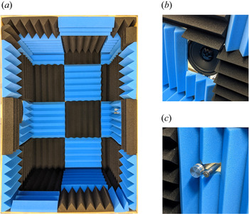
The background noise in the wind tunnel has been removed from the measurements using a Wiener noise cancelling filter. This filter produces an estimate of the background noise and requires a simultaneous measurement of the noise field along with the measurement of wall pressure. This has been accomplished using the second microphone, which was supported in the free stream and fitted with a nose cone. The support structure for this microphone consists of two pieces: one three-dimensional (3-D) printed and one machined from aluminium. The overall design goal of this structure was to permit measurement of the background noise without disturbing the flow. The structure, which is shown schematically in figure 2, supports the microphone in the free stream at  $(x,y,z) = (0,2.1\delta ,-5.4\delta )$. Once the background noise has been estimated using the filter, it is subtracted from the Helmholtz-corrected wall-pressure signal to obtain an estimate of the true wall pressure
 $p$.
Schematic of the experimental set-up. The axes origin is located at the pinhole of microphone 1 and is offset here to not interfere with the fields of view.

2.2. Particle image velocimetry
Three separate PIV experiments have been conducted to capture the velocity field of the present TBL. The field of view (FOV) associated with each experiment is shown schematically in figure 2, where each FOV is numbered accordingly. The same laser and cameras were used for all three experiments. The high-speed laser (Photonics Industries DM20-527-DH) features two separate cavities. The beam from each cavity is capable of 20 mJ per pulse at 1 kHz. The high-speed cameras (Phantom v611) feature a  $1280 \times 800$-pixel complementary metal oxide semiconductor (CMOS) sensor with a
 $20\ \mathrm {\mu }\textrm {m}\times 20\ \mathrm {\mu }\textrm {m}$ pixel size and 12-bit resolution. All PIV experiments were seeded with
 $\sim$1
 $\mathrm {\mu }$m particles using a fog generator. The PIV images were preprocessed in two steps using DaVis 8.4 (LaVision GmbH). First, the minimum of each ensemble was subtracted to reduce the background noise. Second, the images were divided by the background-subtracted ensemble average to normalize the intensity counts.
The FOV denoted as FOV1 in figure 2 was used to capture the flow field from the wall to beyond the height of the TBL for determining  $\delta$,
 $\delta ^*$,
 $\theta$ and
 $U_\infty$. These measurements were therefore not synchronized with wall pressure. A 1-mm-thick laser sheet, formed within FOV1 using a combination of spherical and cylindrical lenses, was used to illuminate the particles. A single camera and a 200-mm lens with an aperture setting of
 $f/5.6$ resulted in a cropped FOV of
 $({{\rm \Delta} }x, {{\rm \Delta} }y) = 47\ \textrm {mm} \times 140$ mm with a resolution of 109.6
 $\mathrm {\mu }$m pixel
 $^{-1}$. A total of 10 000 double-frame images were collected over four sets at an acquisition rate of 25 Hz, corresponding to a total sampling time of
 $5.0{\times }10^{4}\delta /U_\infty$. Following preprocessing, the images were processed in DaVis using a multi-pass cross-correlation algorithm. The final pass employed
 $32 \times 32$-pixel Gaussian-weighted interrogation windows with 75 % overlap.
The FOV denoted as FOV2 in figure 2 was used to capture the coupling between wall pressure and velocity throughout the logarithmic and lower-wake layers of the TBL. The same laser sheet from FOV1 was utilized here. A single camera and a 300-mm lens with an aperture setting of  $f/8$ resulted in a cropped FOV of
 $({{\rm \Delta} }x, {{\rm \Delta} }y) = 9\ \textrm {mm} \times 82$ mm with a resolution of 64.4
 $\mathrm {\mu }$m pixel
 $^{-1}$. The FOV was cropped to be narrow to allow for longer sequences of images to be collected, as the high-speed camera memory is limited and longer sequences are required for convergence of the pressure-velocity cross-statistics. A total of 120 000 double-frame images were collected over eight sets at an acquisition rate of 1 kHz, corresponding to a total sampling time of
 $1.5{\times }10^{4}\delta /U_\infty$. The 1 kHz acquisition rate is sufficient for computing the cross-spectra between wall pressure and velocity while resolving the frequencies of the low-frequency, mid-frequency and overlap regions of the wall-pressure power spectrum associated with the present TBL as will be shown later in § 3.1. The wall pressure and wind tunnel background noise were recorded simultaneously with the PIV images of FOV2, as were the trigger signals of the laser and camera for later synchronization. The PIV images were processed in DaVis as described above for FOV1.
Stereoscopic PIV was conducted in the FOV denoted as FOV3 in figure 2. Two cameras each with a Scheimpflug mount and a 300-mm lens with an aperture setting of  $f/11$ were used. A 2-mm-thick laser sheet was formed within FOV3 using a spherical lens and a collimator. A thicker laser sheet was used here to improve the correlation between double-frame images, as the free stream flow direction is normal to FOV3. Both cameras were placed in a forward-scattering orientation with respect to the laser sheet with 90
 $^\circ$ between their lines of sight. The cameras were calibrated using a two-step process, which included a 3-D target calibration followed by a self-calibration using a small set of particle images (Wieneke Reference Wieneke2005). This resulted in a FOV of
 $({{\rm \Delta} }y, {{\rm \Delta} }z) = 94\ \textrm {mm} \times 188$ mm with an effective resolution of 102.8
 $\mathrm {\mu }$m pixel
 $^{-1}$. Note that the usable wall-normal (
 ${{\rm \Delta} }y$) portion of the FOV is roughly 47 mm due to the height of the laser sheet, which was reduced to retain laser power and obtain a sufficient intensity count in the images. A total of 21 600 double-frame images were collected over eight sets at an acquisition rate of 1 kHz, corresponding to a total sampling time of
 $2.7{\times }10^{3}\delta /U_\infty$. Wall pressure, the wind tunnel background noise and the trigger signals were once again recorded simultaneously with these PIV images for later synchronization. DaVis was used to apply a multi-pass cross-correlation algorithm to the double-frame images using
 $48 \times 48$-pixel Gaussian-weighted interrogation windows with 75 % overlap for the final pass.
3. Previously established statistics
It is important to verify that the present wall-pressure and velocity measurements are reliable before moving forward with the primary analyses in § 4. This is accomplished here by comparing the measurement statistics with those that have been previously established in the literature. Specifically, we will look at single-point velocity statistics (the mean profile, Reynolds stresses and power spectra), single-point wall-pressure statistics (the power spectrum, probability density and root-mean-square value) and space–time pressure-velocity correlations. The uncertainties associated with the statistics that are defined by means, root-mean-square values, variances and covariances are estimated in Appendix B.
3.1. Single-point wall-pressure and velocity statistics
The mean velocity profile and Reynolds stresses, evaluated using each of the three PIV measurements conducted in the present experimental campaign, are displayed on semi-logarithmic axes in figure 3. The mean velocity profiles in figure 3( $a$) are compared with the logarithmic law of the wall with
 $\kappa = 0.41$ and
 $C = 5.0$. The profiles from the three PIV measurements agree well with one another and with the logarithmic law up to approximately
 $y/\lambda = 400$. It is also evident that the viscous sublayer (
 $y/\lambda \lesssim 5$) and buffer layer (
 $5 \lesssim y/\lambda \lesssim 30$) are not captured by the present measurements. This is not an issue for our investigation because the measurements have been optimized to capture the largest motions that occupy the logarithmic and wake layers of the TBL. The Reynolds stresses (excluding the spanwise velocity component) from all three experiments are shown in figure 3(
 $b$). The streamwise normal component from the hotwire measurements of Hutchins & Marusic (Reference Hutchins and Marusic2007a) at
 $Re_\tau = 2630$ is also included for comparison. It can be seen in the figure that the present measurements conducted using planar PIV (FOV1 and FOV2) agree well with one another, and
 $\langle u^2 \rangle /U_\tau ^2$ agrees well with the measurements of Hutchins & Marusic (Reference Hutchins and Marusic2007a). In contrast, some deviation is observed for the stereo-PIV measurements (FOV3). This is attributed to the added uncertainties associated with stereoscopic calibration, particularly with respect to the out-of-plane component (streamwise in this case). Despite this, figure 3(
 $b$) reveals that the Reynolds stresses calculated from stereo-PIV agree reasonably well with those calculated from planar PIV. However, to remain conservative, the use of the present stereo-PIV measurements will be used primarily for qualitative analyses.
Velocity statistics at the pressure measurement location ( $x = z = 0$) from the three PIV experiments: (
 $a$) mean velocity profiles and (
 $b$) Reynolds stresses. The use of
 $\langle \cdots \rangle$ denotes an ensemble average in time. Here H & M (2007) refers to the hotwire measurements of Hutchins & Marusic (Reference Hutchins and Marusic2007a) at
 $Re_\tau = 2630$. The uncertainties associated with these statistics are estimated in Appendix B.

The power spectral density of streamwise velocity fluctuation as a function of wavenumber ( $\phi _u(k_x)$;
 $k_x = 2{{\rm \pi} }f/\langle U(y) \rangle$) has been computed using both sets of high-speed PIV data (FOV2 and FOV3) and is displayed in figure 4 for two wall-normal locations within the logarithmic layer. The spectra have been normalized such that they can be easily compared with the work of Balakumar & Adrian (Reference Balakumar and Adrian2007), who consolidated the spectra from several investigations of various wall-bounded flows with Reynolds numbers similar to that of the present TBL. The spectra of figure 4 show excellent agreement with those shown in Balakumar & Adrian (Reference Balakumar and Adrian2007), including the collapse of the curves in the
 $k^{-1}_x$ region (roughly
 $k^{-1.04}_x$ here). We also see good agreement between the spectra from the planar (FOV2) and stereo (FOV3) data when they are compared at the same wall-normal location. Note that the increase in spectral densities at higher wavenumbers is associated with PIV noise. As we will see later, these higher wavenumbers (frequencies) are not important to the conclusions of the present investigation.
Power spectral density of streamwise velocity fluctuation as a function of wavenumber ( $\phi _u(k_x)$;
 $k_x = 2{{\rm \pi} }f/\langle U(y) \rangle$) computed from the high-speed PIV measurements of FOV2 and FOV3. Note that
 $y/\delta = 0.07$ and 0.14 coincide with roughly
 $y/\lambda = 180$ and 360, respectively.

The power spectral density of wall pressure ( $\phi _p(\omega )$;
 $\omega = 2{{\rm \pi} }f$) is displayed in figure 5 using both inner- and outer-layer normalizations. The frequencies displayed range from 0.7 Hz to 3 kHz, which is the reliable range of measurable frequencies as discussed in § 2.1. The divisions between the low-frequency, mid-frequency, overlap and high-frequency regions of the spectrum as defined by Hwang, Bonness & Hambric (Reference Hwang, Bonness and Hambric2009) are included for reference, revealing that the present wall-pressure measurements capture the frequencies associated with all four regions. The upper frequency captured by the PIV measurements as dictated by the Nyquist criterion (
 ${\leq }500$ Hz) is also displayed, indicating that the PIV measurements resolve the frequencies of the low- and mid-frequency regions and nearly all of the overlap region. The low- and mid-frequency regions collapse over a range of Reynolds numbers when they are non-dimensionalized using outer-layer variables (Farabee & Casarella Reference Farabee and Casarella1991; Tsuji et al. Reference Tsuji, Fransson, Alfredsson and Johansson2007; Klewicki et al. Reference Klewicki, Priyadarshana and Metzger2008), suggesting that these frequencies are caused by the motions of the outer layer. Since both the PIV and wall-pressure measurements capture the entirety of these regions, the synchronized measurements should resolve the large-scale pressure-velocity coupling relevant to this investigation.
Power spectral density of wall pressure ( $\phi _p(\omega )$;
 $\omega = 2{{\rm \pi} }f$) normalized using both inner- and outer-layer variables. The divisions between the four regions of the spectrum are set as defined by Hwang et al. (Reference Hwang, Bonness and Hambric2009). The upper frequency resolved by PIV is dictated by the Nyquist criterion.

The spectrum displayed in figure 5 features the characteristics expected for the wall pressure beneath a TBL (Hwang et al. Reference Hwang, Bonness and Hambric2009). More specifically, the spectrum climbs in magnitude as frequency is increased until a peak is reached in the mid-frequency region. The spectrum then declines in magnitude and passes through two ranges of constant proportionality, one in the overlap region and one in the high-frequency region. The constant decay in the high-frequency region has been observed in the past to be approximately  $\omega ^{-5}$ to
 $\omega ^{-6}$ (McGrath & Simpson Reference McGrath and Simpson1987; Goody Reference Goody2004; Palumbo Reference Palumbo2012; Van Blitterswyk & Rocha Reference Van Blitterswyk and Rocha2017). The presently observed decay of
 $\omega ^{-5.60}$ shown in figure 5 is therefore in good agreement with the literature. The same can be said about the
 $\omega ^{-0.65}$ decay in the overlap region, which is typically observed to be roughly
 $\omega ^{-0.7}$ (McGrath & Simpson Reference McGrath and Simpson1987; Goody Reference Goody2004; Tsuji et al. Reference Tsuji, Fransson, Alfredsson and Johansson2007; Van Blitterswyk & Rocha Reference Van Blitterswyk and Rocha2017). The behaviour of the low-frequency region is not well established at the moment. Some attempts at modelling the wall-pressure spectrum suggest that the low-frequency region should vary with
 $\omega ^2$ as discussed by Panton et al. (Reference Panton, Goldman, Lowery and Reischman1980) and Bull (Reference Bull1996), while another model predicts a
 $\omega ^{1.1}$ to
 $\omega ^{1.5}$ proportionality (Panton & Linebarger Reference Panton and Linebarger1974). There is currently some experimental evidence to support the former (Farabee & Casarella Reference Farabee and Casarella1991; Palumbo Reference Palumbo2012), but reliable low-frequency data are difficult to obtain owing to background noise contamination and frequency response limitations of the available pressure transducers. As is evident in figure 5, the low-frequency region measured here grows with
 $\omega ^{1.07}$ and, therefore, shows better agreement with the work of Panton & Linebarger (Reference Panton and Linebarger1974).
The root-mean-square wall pressure ( $p_{{rms}}$) was calculated by integrating the power spectral density plotted in figure 5 followed by taking the square root. The inner-normalized value is
 $p_{{rms}}/{\rho }U_\tau ^2 = 3.16$, which represents an error of only 1.7 % when compared with the empirical relation derived by Farabee & Casarella (Reference Farabee and Casarella1991). This relation is
 $(p_{{rms}}/{\rho }U_\tau ^2)^2 = 6.5 + 1.86 \ln (Re_{\tau }/333)$ for
 $Re_{\tau } > 333$ and has been found to agree well with direct numerical simulations and experiments for
 $Re_\tau$ up to roughly 20 000 (Tsuji et al. Reference Tsuji, Fransson, Alfredsson and Johansson2007, Reference Tsuji, Imayama, Schlatter, Alfredsson, Johansson, Marusic, Hutchins and Monty2012). The present wall-pressure fluctuations have a skewness of 0.056 and a flatness of 4.39, which agree with the values reported by Schewe (Reference Schewe1983), Tsuji et al. (Reference Tsuji, Fransson, Alfredsson and Johansson2007) and Naka et al. (Reference Naka, Stanislas, Foucaut, Coudert, Laval and Obi2015). The probability density of the present wall-pressure measurements normalized by
 $p_{{rms}}$ is plotted on linear and semi-logarithmic axes in figures 6(
 $a$) and 6(
 $b$), respectively. Here, the dashed line is a Gaussian fit to the data for comparison. The approximate envelope of values reported by Tsuji et al. (Reference Tsuji, Fransson, Alfredsson and Johansson2007) for
 $5870 \leq Re_\theta \leq 16\ 700$ is also shown on the semi-logarithmic axes in figure 6(
 $b$) using a grey outline. Since the extreme tails of the probability density functions in Tsuji et al. (Reference Tsuji, Fransson, Alfredsson and Johansson2007) exhibit large amounts of scatter, the envelope depicts the range of values that we expect the functions to fall within. When looking at the probability density on linear axes in figure 6(
 $a$), we can see that the measured density clearly deviates from the Gaussian fit at the peak and for densities ranging from roughly 0.05 to 0.2. This same deviation is visible in the results of Schewe (Reference Schewe1983) and Tsuji et al. (Reference Tsuji, Fransson, Alfredsson and Johansson2007). An even larger deviation from Gaussian behaviour is visible when looking at the semi-logarithmic axes in figure 6(
 $b$). This deviation occurs at the extreme tails of the distribution and is indicative of the HAPPs in wall-pressure fluctuation that have been studied in the past (Johansson et al. Reference Johansson, Her and Haritonidis1987; Karangelen et al. Reference Karangelen, Wilczynski and Casarella1993; Kim et al. Reference Kim, Choi and Sung2002; Ghaemi & Scarano Reference Ghaemi and Scarano2013). As is evident in the figure, the tails of the present probability density function fall within the approximate envelope of values from Tsuji et al. (Reference Tsuji, Fransson, Alfredsson and Johansson2007).
Measured probability density of wall-pressure fluctuations compared with a Gaussian fit of the same data; shown on ( $a$) linear and (
 $b$) semi-logarithmic axes. The grey outline in (
 $b$) is the approximate envelope of values reported by Tsuji et al. (Reference Tsuji, Fransson, Alfredsson and Johansson2007) for
 $5870 \leq Re_\theta \leq 16\ 700$.

3.2. Space–time pressure-velocity correlations
We now employ space–time pressure-velocity correlations along with Taylor's hypothesis to investigate the spatial correlation between wall pressure and velocity throughout the TBL. This is done to compare the present pressure-velocity coupling with the results of Buchmann et al. (Reference Buchmann, Kücükosman, Ehrenfried and Kähler2016) and Naka et al. (Reference Naka, Stanislas, Foucaut, Coudert, Laval and Obi2015) and to establish baselines for later comparison within the present study. Note that Dennis & Nickels (Reference Dennis and Nickels2008) evaluated the accuracy of using Taylor's hypothesis to construct spatial fields in a TBL and showed that the majority of the large-scale errors occur for extrapolations beyond roughly  $\pm 3.5\delta$ from the measurement location. As we will see, the main features of all correlations computed in this investigation fall within this range and, therefore, we can apply Taylor's hypothesis here.
We define the space–time pressure-velocity correlation as
 \begin{equation} {\boldsymbol{R}}_{pu_i}({{\rm \Delta}}t,y,z) = \frac{1}{{\rho}U^3_\infty}\langle p(t)u_i(t-{{\rm \Delta}}t,0,y,z) \rangle, \end{equation}
where  $u_i$,
 $i = 1$, 2, 3, are the fluctuating velocity components and the use of
 $\langle \cdots \rangle$ denotes an ensemble average in time. We normalize the correlations using
 ${\rho }U^3_\infty$ to remain consistent with Naka et al. (Reference Naka, Stanislas, Foucaut, Coudert, Laval and Obi2015). The correlations have also been computed using only
 $p>0$ and
 $p<0$ to isolate the motions associated with positive and negative wall-pressure fluctuations. We denote these two conditional cases as
 ${\boldsymbol {R}}^+_{pu_i} = {\boldsymbol {R}}_{pu_i}|_{p>0}$ and
 ${\boldsymbol {R}}^-_{pu_i} = {\boldsymbol {R}}_{pu_i}|_{p<0}$.
Equation (3.1) was applied separately to the PIV snapshots from FOV2 and FOV3 and then Taylor's hypothesis was used to transform  ${{\rm \Delta} }t$ into streamwise distance using the local convection velocity
 $U_c$. Here we set
 $U_c$ as the mean streamwise velocity at the corresponding wall-normal location, as the mean has been shown to closely match the convection velocity for
 $y>0.05\delta$ (Lee & Sung Reference Lee and Sung2011). This technique was employed to avoid the non-physical streamwise stretching and compression of the correlations that can occur when a single convection velocity is chosen for use with Taylor's hypothesis. Since each wall-normal location is associated with a different
 $U_c$, the streamwise extent of the correlation at each
 $y$ is different. Interpolation has therefore been used to form a common
 ${{\rm \Delta} }tU_c$ grid for plotting. On this grid,
 ${{\rm \Delta} }tU_c<0$ represents upstream from the pressure measurement location, while
 ${{\rm \Delta} }tU_c>0$ represents downstream. Finally, the symmetry (and antisymmetry) of these correlations about the
 $z=0$ plane was exploited to improve the convergence of the results computed using the stereo-PIV measurements of FOV3. This was accomplished by flipping each component of the correlation about
 $z=0$, adding it to the original (or subtracting in the case of antisymmetry), and then dividing the result by 2. The outcome of this procedure is that the results appear perfectly symmetric (or antisymmetric) about
 $z=0$ with the benefit of reduced noise.
Plots of  ${\boldsymbol {R}}_{pu_i}$,
 ${\boldsymbol {R}}^+_{pu_i}$ and
 ${\boldsymbol {R}}^-_{pu_i}$ in streamwise–wall-normal planes are given in figure 7. The streamwise and wall-normal components of the correlations are plotted at
 $z = 0$, while the spanwise component is at
 $z/\delta = 0.2$ to match the plane location plotted by Naka et al. (Reference Naka, Stanislas, Foucaut, Coudert, Laval and Obi2015). Note that this plane must be offset in the spanwise direction because
 ${\boldsymbol {R}}_{pw}$ is antisymmetric about the
 $z=0$ plane and is therefore zero within it. In general, the shapes, sizes and magnitudes of the correlations are in good agreement with those of Buchmann et al. (Reference Buchmann, Kücükosman, Ehrenfried and Kähler2016) and Naka et al. (Reference Naka, Stanislas, Foucaut, Coudert, Laval and Obi2015), with a few exceptions that will be detailed shortly.
Space–time pressure-velocity correlations ( ${\boldsymbol {R}}_{pu_i}$) as defined by (3.1) calculated using the (
 $a$) streamwise, (
 $b$) wall-normal and (
 $c$) spanwise velocity components. The superscripts ‘
 $+$’ and ‘
 $-$’ denote correlations computed using only
 $p>0$ or
 $p<0$, respectively. The streamwise–wall-normal planes in (
 $a$) and (
 $b$) are located at
 $z = 0$, while those in (
 $c$) are located at
 $z = 0.2\delta$. The plots in (
 $c$) do not cover as much of the wall-normal distance due to the limitations of FOV3. The uncertainties associated with these correlations are estimated in Appendix B.

The contours of  ${\boldsymbol {R}}_{pu}$ in figure 7(
 $a$) reveal that
 $p$ is positively correlated with
 $u$ directly above the pressure measurement location throughout nearly the whole boundary layer thickness and extending upstream to
 ${{\rm \Delta} }tU_c/\delta \approx -3$. Two regions of weaker negative correlation between
 $p$ and
 $u$ extend downstream. The first region begins just past the pressure measurement location and extends at an angle from the wall to reach
 ${{\rm \Delta} }tU_c/\delta \approx 2.3$ and
 $y/\delta \approx 0.7$. The second region sits close to the wall and reaches to
 ${{\rm \Delta} }tU_c/\delta \approx 8$ (not entirely shown to keep the figure manageable). These same features are visible in the correlations of both Buchmann et al. (Reference Buchmann, Kücükosman, Ehrenfried and Kähler2016) and Naka et al. (Reference Naka, Stanislas, Foucaut, Coudert, Laval and Obi2015), although there are some differences in the sizes of the features between all three studies. The results of Naka et al. (Reference Naka, Stanislas, Foucaut, Coudert, Laval and Obi2015) suggest that these size differences could be Reynolds number effects. When we consider
 ${\boldsymbol {R}}^+_{pu}$, the region of positive correlation and the second region of negative correlation both become larger and more intense, while the first region of negative correlation disappears. The intensified region of positive correlation now extends across the range
 $-4 \lesssim {{\rm \Delta} }tU_c/\delta \lesssim 1$, making its total streamwise extent
 ${\sim }5\delta$. In contrast, the intensified region of negative correlation extends to roughly
 ${{\rm \Delta} }tU_c/\delta \approx 8.5$. The contours of
 ${\boldsymbol {R}}^-_{pu}$ show the opposite change to what was observed for
 ${\boldsymbol {R}}^+_{pu}$; the first region of negative correlation has grown larger and more intense while the other two regions have become smaller and weaker. A second region of weak positive correlation has also emerged within the correlations, this time extending downstream at an angle from the wall to
 ${{\rm \Delta} }tU_c/\delta \approx 5$.
Figure 7( $b$) reveals that the contours of
 ${\boldsymbol {R}}_{pv}$ are nearly antisymmetric about
 ${{\rm \Delta} }tU_c=0$. The upstream region shows a negative correlation between
 $p$ and
 $v$, while the downstream region shows a positive correlation which is slightly weaker than the former but comparable in size. The contours extend to
 ${{\rm \Delta} }tU_c/\delta \approx \pm 1.5$ and appear to reach the full height of the boundary layer. The same correlation in Naka et al. (Reference Naka, Stanislas, Foucaut, Coudert, Laval and Obi2015) shows more differences between the sizes of the two lobes of correlation but are overall in good agreement with the present results. Comparison with Buchmann et al. (Reference Buchmann, Kücükosman, Ehrenfried and Kähler2016) is not possible because only the streamwise component of the correlation was reported in their study. When we consider
 ${\boldsymbol {R}}_{pv}^+$, the upstream region of correlation becomes more intense and the downstream region less intense; the opposite is true for
 ${\boldsymbol {R}}_{pv}^-$. This too is observed in the results of Naka et al. (Reference Naka, Stanislas, Foucaut, Coudert, Laval and Obi2015). When
 ${\boldsymbol {R}}_{pu}$ and
 ${\boldsymbol {R}}_{pv}$ are considered together, it is evident that the motions that are most highly correlated with wall pressure generally have
 $u$ and
 $v$ components of opposite sign. This indicates that sweeps and ejections are an important feature of the pressure-velocity coupling.
Finally, the contours of  ${\boldsymbol {R}}_{pw}$ at
 $z/\delta =0.2$ are given in figure 7(
 $c$). The contours indicate that the spanwise motions associated with wall pressure occupy up to at least
 $y/\delta =0.5$. A region of positive correlation between
 $p$ and
 $w$ sits above
 ${{\rm \Delta} }tU_c/\delta = 0$ and has a total streamwise extent of
 ${\sim }1.5\delta$. The region of positive correlation is attached and inclined to the wall and sits between two weaker regions of negative correlation, both of which also have streamwise extents of
 ${\sim }1.5\delta$. The upstream region of negative correlation is away from the wall and extends horizontally across the mid-region of the boundary layer. The downstream region of negative correlation is narrow, inclined and attached to the wall. When considering
 ${\boldsymbol {R}}_{pw}^+$, the region of positive correlation and the upstream region of negative correlation both become stronger, while the downstream region of negative correlation disappears. When considering
 ${\boldsymbol {R}}_{pw}^-$, the downstream region of negative correlation becomes stronger, the region of positive correlation becomes smaller, and the upstream region of negative correlation nearly disappears. These correlations are again consistent with the results of Naka et al. (Reference Naka, Stanislas, Foucaut, Coudert, Laval and Obi2015).
The regions of positive and negative correlation in figure 7( $c$) feature spanwise motion in opposite directions. When coupled with the wall-normal component of the correlations, it is evident that these patterns are associated with quasi-streamwise rotational motions. For example, when looking immediately downstream from the pressure measurement location,
 ${\boldsymbol {R}}_{pu_i}^-$ shows spanwise motion towards
 $z=0$ near the wall, upward motion around
 $z=0$, and motion away from
 $z=0$ farther from the wall to form a rotational pattern. The downstream interface between positive and negative correlation in
 ${\boldsymbol {R}}_{pw}^-$ is therefore related to the rotational axes of an inclined vortical motion as is labelled in figure 7(
 $c$). Similarly, the upstream interface between positive and negative correlation in
 ${\boldsymbol {R}}_{pw}^+$ is associated with a vortical motion that is more horizontal. Because of the symmetry of
 ${\boldsymbol {R}}_{pv}$ and antisymmetry of
 ${\boldsymbol {R}}_{pw}$ (about
 $z=0$), these vortical motions exist as counter-rotating pairs. This observation also supports the coupling between ejection/sweeping motions and wall pressure, as these motions are often induced by quasi-streamwise vortices.
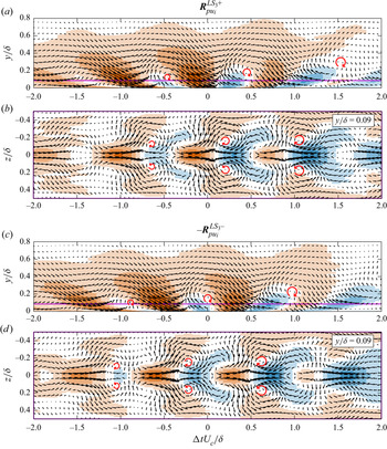
All components of  ${\boldsymbol {R}}^+_{pu_i}$ and
 ${\boldsymbol {R}}^-_{pu_i}$ can be used to visualize the motions and vortical structures associated with positive and negative wall-pressure fluctuations by forming vector fields from the correlations. These visualizations are presented in figure 8, where the background shows the streamwise component of the correlations using the same colour scaling as figure 7(
 $a$). Note that the correlations for negative wall-pressure fluctuations have been multiplied by
 $-1$ so that the vector directions represent the true flow direction in the visualization. Figure 8(
 $a$,
 $d$) show the streamwise–wall-normal plane of the corresponding vector field at
 $z=0$. These subfigures are marked with vertical lines which represent the locations of spanwise–wall-normal planes that are plotted directly below. The locations of these planes have been selected to show the most important features of each field. The vector density has been decimated and the vector lengths in the spanwise–wall-normal planes have been increased to improve the visualizations.
Visualizations of the vector fields associated with ( $a$–
 $c$)
 ${\boldsymbol {R}}^+_{pu_i}$ and (
 $d$–
 $f$)
 $-{\boldsymbol {R}}^-_{pu_i}$. The background colour represents the streamwise component of the correlations and has the same scaling as figure 7(
 $a$). The coloured lines in (
 $a$,
 $d$) show the locations of the spanwise–wall-normal planes that are plotted directly below. The vector lengths in (
 $b$,
 $c$,
 $e$,
 $\,f$) have been altered relative to those in (
 $a$,
 $d$) to improve the visualizations.

The visualization of  ${\boldsymbol {R}}^+_{pu_i}$ shown in figure 8(
 $a$–
 $c$) reveals that positive wall-pressure fluctuations are associated with an elongated high-speed region with a relatively strong sweeping motion at its leading edge. This sweep is flanked by large low-speed zones and counter-rotating streamwise vortical motions, both of which can be seen in figure 8(
 $b$); these vortical motions are nearly horizontal as is evident in the correlation patterns of
 ${\boldsymbol {R}}^+_{pw}$ shown in figure 7(
 $c$). A first-quadrant event, i.e. a motion with positive
 $u$ and
 $v$, exists downstream from the large sweep as can be seen in figure 8(
 $a$,
 $c$). The visualization of
 $-{\boldsymbol {R}}^-_{pu_i}$ shown in figure 8(
 $d$–
 $f$) indicates that negative wall-pressure fluctuations are associated with a localized upstream ejection and an elongated downstream sweep. This particular sweep sits away from the wall over most of its length. Figure 8(
 $e$) shows that the upstream ejection in not associated with counter-rotating vortex pairs, while figure 8(
 $f$) shows that the downstream sweep is; these vortical motions are more strongly inclined with respect to the wall as is indicated in the patterns of
 ${\boldsymbol {R}}^-_{pw}$ shown in figure 7(
 $c$).
The motions visualized in figure 8 are consistent with those discussed by Naka et al. (Reference Naka, Stanislas, Foucaut, Coudert, Laval and Obi2015). However, they are not a satisfying description of the large-scale pressure-velocity coupling because it is difficult to find clear patterns of hairpin packets or VLSMs by inspection of these visualizations. This is because the correlations represent a superposition of many coherent structures of varying types, sizes and locations. We therefore conclude that the flow patterns of figure 8 are manifestations of the averaging process of the correlations. As we will see in the following sections, decomposing these correlations using different wall-pressure frequency bands yields simpler parts that are interpretable in terms of the large-scale coherent structures that are known to exist within TBLs.
4. Frequency-dependent pressure-velocity coupling
We now move on to the primary analyses of the present work. Our goal here is to scrutinize the coupling between the fluctuating wall pressure and velocity throughout the TBL as a function of frequency. As we will see, there are two distinct coupling mechanisms at the lower frequencies that affect different frequency bands. We first identify these bands using estimates of the coherence between wall pressure and velocity. We then extract the space–time pressure-velocity correlations associated with each band to expose the underlying coherent structures responsible for the observed coupling. The uncertainties associated with these correlations are estimated in Appendix B.
4.1. Coherence between wall pressure and velocity
The cross-spectrum between wall pressure and velocity will allow us to study the pressure-velocity coupling as a function of frequency. Here we employ a normalized form of the cross-spectral density known as the magnitude-squared coherence, which will simply be referred to as the coherence moving forward. The coherence between the fluctuating wall pressure  $p$ and a fluctuating velocity component
 $u_i$ is defined as
 \begin{equation} {\boldsymbol{C}}_{pu_i}(\omega,y) = \frac{|\phi_{pu_i}(\omega,y)|^2}{\phi_p(\omega)\phi_{u_i}(\omega,y)},\end{equation}
where  $\phi _{pu_i}(\omega ,y)$ is the cross-spectral density between
 $p(t)$ and
 $u_i(t,0,y,0)$, and
 $\phi _{u_i}(\omega ,y)$ is the power spectral density of
 $u_i(t,0,y,0)$. Equation (4.1) is estimated here using Welch's overlapping segment method. The coherence function is bounded by 0 and 1, with 0 representing no correlation between the two signals at a given frequency. A coherence of 1 occurs when the two signals are related through a single-input single-output linear, time-invariant system. The latter will never be realized for a turbulent flow due to the nonlinearity and multiple inputs of the governing equations, but the coherence will allow us to probe any coupling that may exist between wall pressure and velocity.
The estimated coherence between wall pressure and the fluctuating velocity components  $u$ and
 $v$ for the wall-normal range of FOV2 are presented on logarithmic axes in figure 9(a,b). The power spectral density of wall pressure is included in figure 9(
 $c$) with the frequency axis aligned to those showing
 ${\boldsymbol {C}}_{pu_i}$ for reference. When looking at figure 9(
 $a$), it is immediately apparent that there are two separate regions of high coherence with distinct characteristics. We demarcate these two regions using the dotted vertical lines in the figure at
 $\omega \delta /U_\infty =0.9$ (17.5 Hz) and 8.0 (160 Hz). These demarcations were selected by visual inspection of the coherence patterns. Note that there is a slight overlap in frequencies for which the first region of high-coherence transitions to the second and, therefore, the interface separating the two regions is not a straight vertical line. Despite this, we have selected the single frequency of
 $\omega \delta /U_\infty =0.9$ as the division between these two regions to simplify the analysis moving forward. The upper frequency of the second region of high coherence was selected as the point at which the coherence drops below
 ${\sim }0.05$ in figure 9(
 $b$).
Estimated coherence between wall pressure and velocity fluctuation ( ${\boldsymbol {C}}_{pu_i}$) as a function of wall-normal distance as defined by (4.1) for the (
 $a$) streamwise and (
 $b$) wall-normal velocity components. Computed using the high-speed PIV measurements from FOV2. The power spectral density (
 $\phi _p(\omega )$) normalized by outer-layer variables is shown in (
 $c$) with the frequency axis aligned for reference.

The first coherent region in figure 9( $a$), defined by
 $\omega \delta /U_\infty <0.9$, reveals high coherence between
 $p$ and
 $u$ for wall-normal locations up to roughly
 $y/\lambda =1300$ (
 ${\sim }0.5\delta$). In contrast, for the same frequencies, the coherence between
 $p$ and
 $v$ in figure 9(
 $b$) is much weaker. This suggests that low frequency
 $u$ occupying half the boundary layer thickness correlates with low-frequency wall pressure. To estimate the size of the structures associated with the first coherent region, we assume that the convection velocity of these structures is the mean velocity at the half-height of the coherent region (
 $y/\lambda =650$;
 $y=0.25\delta$), corresponding to
 $U_c\approx 0.82U_\infty$. A pressure disturbance convecting at this velocity would need to have a wavelength of
 ${\sim }6\delta$ to produce the upper cutoff frequency of
 $\omega \delta /U_\infty =0.9$. Note that one full wavelength would be made up of a positive structure (
 $p>0$) followed by a negative structure (
 $p<0$) to produce a pattern similar to a sinusoid. The first coherent region therefore seems to be associated with high- and low-pressure structures occupying up to
 ${\sim }0.5\delta$ in height and extending more than
 $3\delta$ in length. This is consistent with the VLSMs and, for this reason, we will refer to the pressure fluctuations in the first coherent region as the very-large-scale pressure (VLSP) fluctuations as labelled in figure 9(
 $c$).
We will now consider the second region of high coherence in figure 9 defined by  $0.9<\omega \delta /U_\infty <8.0$. This region is markedly different than the one associated with the VLSP fluctuations. First, a higher coherence is observed between
 $p$ and
 $v$ than between
 $p$ and
 $u$, although the latter is still quite strong. Second, the region sits at an angle, with lower frequencies associated with locations farther from the wall. This is reminiscent of the attached-eddy hypothesis, as larger attached eddies that extend farther from the wall would be associated with lower frequencies due to the size of the pressure disturbance that they produce. Finally, the second region of high coherence between
 $p$ and
 $v$ extends farther from the wall than the coherence of the VLSP, surpassing the maximum captured by FOV2 (
 ${\sim }0.8\delta$). It is possible that
 ${\boldsymbol {C}}_{pv}$ reaches the full height of the boundary layer, and this is not observed for
 ${\boldsymbol {C}}_{pu}$. This suggests that the pressure fluctuations associated with this region are stronger than the VLSP fluctuations, as they appear to influence the wall pressure from a greater wall-normal distance. To estimate the size of the structures associated with the upper cutoff frequency of the second region of high coherence (
 $\omega \delta /U_\infty =8.0$), we assume a convection velocity of
 $U_c=0.74U_\infty$. This is the mean velocity at
 $y/\lambda =300$, which is roughly the mid-point of the high-coherence region at the upper cutoff as is visible in figure 9(
 $b$). A pressure disturbance convecting at this velocity would need to have a wavelength of
 ${\sim }0.6\delta$ to reproduce the cutoff frequency of
 $\omega \delta /U_\infty =8.0$. We therefore conclude, using the same logic invoked for VLSP, that the second region of high coherence seems to be associated with high- and low-pressure structures with streamwise dimensions ranging from roughly
 $0.3\delta$ to
 $3\delta$. We can consider this range of eddy sizes as being large scale and, therefore, the wall-pressure fluctuations associated with the second region of high coherence will be referred to as the large-scale pressure (LSP) fluctuations as labelled in figure 9(
 $c$).
It is interesting to note that the demarcation between VLSP and LSP coincides with the peak of the wall-pressure spectrum as is evident in figure 9( $c$). The location of the peak, and the different proportionality behaviours on either side, may therefore be associated with a transition between wall-pressure sources, as
 ${\boldsymbol {C}}_{pu_i}$ indicates that different motions are responsible for the wall pressure in the frequency bands on either side of
 $\omega \delta /U_\infty =0.9$. The nature of these two types of motions will be determined in §§ 4.2 and 4.3. It should also be noted that the two frequency cutoffs do not coincide with the transition between any of the regions of the wall-pressure power spectrum shown in figure 5. It can be seen in the figure that
 $\omega \delta /U_\infty = 0.9$ is roughly one-quarter of the way through the mid-frequency region, while
 $\omega \delta /U_\infty = 8.0$ is roughly one-third of the way through the overlap region.
We now investigate the estimated phase between  $p$ and
 $u_i$ from the cross-spectral densities, denoted as
 $\angle \phi _{pu_i}(\omega )$. These estimates are given in figure 10 for the same domain shown for the coherence estimates, and the demarcations for the LSP and VLSP bands are included for reference. Here, a positive phase indicates that
 $p$ leads
 $u_i$, while a negative phase indicates that
 $p$ lags
 $u_i$. The noisy region in the top right corner of both subfigures is due to the general lack of coherence between
 $p$ and
 $u_i$ at high frequencies and wall-normal locations as can be seen in figure 9. A cursory glance at figure 10 makes it clear that
 $\angle \phi _{pu}(\omega )$ is always positive in the regions of non-zero coherence, while
 $\angle \phi _{pv}(\omega )$ is always negative. This is in agreement with the space–time pressure-velocity correlations of figure 7, which show that the positive peak of
 ${\boldsymbol {R}}_{pu}$ always exists upstream from the wall-pressure measurement location (i.e.
 $p$ leads
 $u$), and that the positive peak of
 ${\boldsymbol {R}}_{pv}$ always exists downstream (i.e.
 $p$ lags
 $v$). Focusing now on the region of high coherence within the LSP band of figure 9, we can see that figure 10(
 $a$) indicates a phase varying from roughly
 $0.25{\rm \pi}$ to
 $0.35{\rm \pi}$ between
 $p$ and
 $u$, while figure 10(
 $b$) indicates a phase of roughly
 $-0.5{\rm \pi}$ to
 $-0.6{\rm \pi}$ between
 $p$ and
 $v$. In contrast, the region of high coherence within the VLSP band of figure 9 shows different behaviour. Here, we can see a phase of roughly
 $0.1{\rm \pi}$ to
 $0.25{\rm \pi}$ between
 $p$ and
 $u$, and a phase of roughly
 $-0.7{\rm \pi}$ to
 $-0.8{\rm \pi}$ between
 $p$ and
 $v$. These results support the notion that different mechanisms are responsible for the observed coupling in the LSP and VLSP bands.
Estimated phase between wall pressure and velocity fluctuation ( $\angle \phi (\omega )_{pu_i}$) as a function of wall-normal distance for the (
 $a$) streamwise and (
 $b$) wall-normal velocity components. Computed using the measurements from FOV2. A positive phase indicates that
 $p$ leads
 $u_i$, while a negative phase indicates that
 $p$ lags
 $u_i$.

We have further evaluated the characteristics of the LSP and VLSP fluctuations by applying filters to isolate the associated frequencies. A low-pass filter with a cutoff frequency of  $\omega \delta /U_\infty = 0.9$ was used to isolate the VLSP, and a bandpass filter with cutoffs of
 $\omega \delta /U_\infty = 0.9$ and 8.0 was used to isolate the LSP. These filters were designed as digital finite impulse response filters with the cutoff frequencies placed at
 $-6$ dB attenuation. The filter slopes were made as steep as possible while keeping the filters numerically tractable. We refer to these two filtered signals as
 $p_{LS}$ and
 $p_{VLS}$.
The probability density functions of  $p_{LS}$ and
 $p_{VLS}$ are compared with that of the full spectrum in figure 11. The functions are displayed on linear and semi-logarithmic axes and are compared with Gaussian fits for reference. The horizontal axes are normalized using
 $p_{{rms}}$ of the full spectrum in all cases. Figure 11(
 $a$) reveals that the peak probability density of
 $p_{VLS}$ is more than four times that of the full spectrum, while the peak for
 $p_{LS}$ is not quite double. This indicates that the wall-pressure fluctuations within these two frequency bands are lower in magnitude in general, with the
 $p_{VLS}$ having the lowest magnitudes. More precisely, the root-mean-square value of
 $p_{LS}$ and
 $p_{VLS}$ are 53 % and 20 % of
 $p_{{rms}}$, respectively. This is consistent with the results of Beresh et al. (Reference Beresh, Henfling and Spillers2013), who found that low-frequency wall-pressure fluctuations are weaker than high-frequency wall-pressure fluctuations. Figure 11(
 $a$) also reveals that
 $p_{LS}$ deviates slightly from the Gaussian fit at the peak, while
 $p_{VLS}$ does not. Figure 11(
 $b$) reveals some deviation from Gaussian at the extreme tails for
 $p_{LS}$, but this is again not observed for
 $p_{VLS}$, which appears to adhere to Gaussian behaviour at all amplitudes. We therefore conclude that the VLSP fluctuations are Gaussian, while the LSP fluctuations are nearly Gaussian.
Probability density of the full spectrum of wall-pressure fluctuations compared with that of the LSP and VLSP fluctuations shown on ( $a$) linear and (
 $b$) semi-logarithmic axes. The dashed lines represent Gaussian fits to the same data. All curves are normalized using
 $p_{{rms}}$, the root-mean-square value of the full spectrum of fluctuations.

4.2. Very-large-scale coupling
In the previous section the coherence function between wall pressure and fluctuating velocity revealed two distinct frequency bands of high coherence which appear to be associated with structures with lengths ranging from roughly  $0.3\delta$ to
 $3\delta$ for one band and lengths greater than
 $3\delta$ for the other. We therefore refer to these bands as the LSP and VLSP fluctuations, respectively, and we denote their pressure signals as
 $p_{LS}$ and
 $p_{VLS}$. Within this section, we further investigate the pressure-velocity coupling associated with the VLSP band. The coupling observed in the LSP band will be investigated in § 4.3.
We revisit the space–time pressure-velocity correlations computed in § 3.2, but this time using  $p_{VLS}$ in place of
 $p$. By using only
 $p_{VLS}$ to compute the correlations, we are isolating the motions that cause these fluctuations and, therefore, we are extracting the portion of
 ${\boldsymbol {R}}_{pu_i}$ associated with the VLSP band. We define the space–time pressure-velocity correlation associated with the VLSP band as
 ${\boldsymbol {R}}_{pu_i}^{{VLS}} = {\boldsymbol {R}}_{pu_i}|_{p=p_{VLS}}$ following (3.1) where
 $p_{VLS}$ has been isolated using a low-pass filter as described in § 4.1. We also consider the correlations computed using only
 $p_{VLS}>0$ or
 $p_{VLS}<0$ to isolate the motions associated with each sign of fluctuation. These conditional cases are denoted as
 ${\boldsymbol {R}}_{pu_i}^{{VLS}+} = {\boldsymbol {R}}_{pu_i}^{{VLS}}|_{p_{VLS}>0}$ and
 ${\boldsymbol {R}}_{pu_i}^{{VLS}-} = {\boldsymbol {R}}_{pu_i}^{{VLS}}|_{p_{VLS}<0}$.
We begin by considering the streamwise–wall-normal slices of  ${\boldsymbol {R}}_{pu_i}^{{VLS}}$,
 ${\boldsymbol {R}}_{pu_i}^{{VLS}+}$ and
 ${\boldsymbol {R}}_{pu_i}^{{VLS}-}$ in figure 12. The streamwise and wall-normal components are plotted at
 $z = 0$, while the spanwise component is plotted at
 $z/\delta =0.2$. Note that the colourbar scaling is reduced compared with that of
 ${\boldsymbol {R}}_{pu_i}$ in figure 7 because the correlations magnitudes are considerably weaker, especially for the wall-normal and spanwise components. This is likely because the wall-pressure fluctuations in the VLSP band are five times weaker than those of the full spectrum as was shown in figure 11.
( $a$) Streamwise, (
 $b$) wall-normal and (
 $c$) spanwise components of the space–time pressure-velocity correlations computed using pressure filtered to isolate the VLSP fluctuations (
 ${\boldsymbol {R}}_{pu_i}^{{VLS}} = {\boldsymbol {R}}_{pu_i}|_{p=p_{{VLS}}}$) following (3.1). The superscripts ‘
 $+$’ and ‘
 $-$’ denote correlations computed using only
 $p_{{VLS}}>0$ or
 $p_{{VLS}}<0$, respectively. The streamwise–wall-normal planes in (
 $a$) and (
 $b$) are located at
 $z = 0$, while those in (
 $c$) are located at
 $z = 0.2\delta$. The plots in (
 $c$) do not cover as much of the wall-normal distance due to the limitations of FOV3. The uncertainties associated with these correlations are estimated in Appendix B.

Figure 12 makes it immediately apparent that the motions most correlated with the VLSP fluctuations are unlike those captured by the correlations computed using the full wall-pressure spectrum. The contours of  ${\boldsymbol {R}}_{pu}^{{VLS}}$ displayed in figure 12(
 $a$) reveal that
 $p_{VLS}$ is positively correlated with
 $u$ over a large streamwise extent of
 $-3.8 \lesssim {{\rm \Delta} }tU_c/\delta \lesssim 1.8$ and reaching beyond
 $y/\delta =0.8$ in height. A much smaller and weaker region of negative correlation exists upstream, and a somewhat weaker but highly elongated region of negative correlation extends far downstream from the positively correlated region. The entirety of these regions are not shown in figure 12(
 $a$) to keep the figure manageable. However, we note that the upstream region of weak negative correlation exists between
 $-6.6\lesssim {{\rm \Delta} }tU_c/\delta \lesssim -4.2$, and the downstream region extends to upwards of
 ${{\rm \Delta} }tU_c/\delta \approx 12$. This latter region of correlation seems to be the source of the highly elongated, wall-attached region of negative correlation visible in the contours of
 ${\boldsymbol {R}}_{pu}$ and
 ${\boldsymbol {R}}^+_{pu}$ shown in figure 7(
 $a$). In contrast to the correlations computed using the full wall-pressure spectrum, the contours of
 ${\boldsymbol {R}}_{pu}^{{VLS}+}$ and
 ${\boldsymbol {R}}_{pu}^{{VLS}-}$ remain largely unchanged relative to
 ${\boldsymbol {R}}_{pu}^{{VLS}}$.
Figure 12( $b$) reveals a large region of negative correlation in the contours of
 ${\boldsymbol {R}}_{pv}^{{VLS}}$. This region extends through the range
 $-4.3 \lesssim {{\rm \Delta} }tU_c/\delta \lesssim 1.1$, exceeds
 $y/\delta = 0.8$, and has a different shape overall when compared with that of
 ${\boldsymbol {R}}_{pu}^{{VLS}}$. Regions of weaker positive correlation with similar shapes sit immediately upstream and downstream from this region of negative correlation, revealing a clear alternating pattern. The coherence estimates of figure 9 showed a much higher coherence between
 $p_{VLS}$ and
 $u$ than between
 $p_{VLS}$ and
 $v$. This is also apparent in the present correlations, as
 ${\boldsymbol {R}}_{pv}^{{VLS}}$ is approximately four times weaker than
 ${\boldsymbol {R}}_{pu}^{{VLS}}$. In addition, the contours of
 ${\boldsymbol {R}}_{pv}^{{VLS}+}$ and
 ${\boldsymbol {R}}_{pv}^{{VLS}-}$ also appear to remain relatively unchanged compared with
 ${\boldsymbol {R}}_{pv}^{{VLS}}$, just as was the case for the streamwise component. The regions of high correlation that overlap between
 ${\boldsymbol {R}}_{pu}^{{VLS}}$ and
 ${\boldsymbol {R}}_{pv}^{{VLS}}$ reveal that the motions most correlated with
 $p_{VLS}$ feature
 $u$ and
 $v$ of opposite sign. However, these motions are different from sweeps and ejections, which are typically more localized and intense. Instead, these motions appear to be large-scale high- and low-speed streaks with relatively weak wall-normal velocity components.
The wall-normal velocity visible in  ${\boldsymbol {R}}_{pv}^{{VLS}}$ is supported by the contours of
 ${\boldsymbol {R}}_{pw}^{{VLS}}$ in figure 12(
 $c$). The near-wall region of strong positive correlation within the subfigure indicates that there is fluid motion away from
 $z=0$ beneath the high-speed streaks (splatting) and motion towards
 $z=0$ beneath the low-speed streaks (an influx to replace the fluid being lifted). Additionally, a region of weaker negative correlation with a similar streamwise extent exists upstream from the region of positive correlation. A large portion (
 $\sim$3–
 $4\delta$) of these two regions of opposite correlation overlap in the streamwise direction, forming a region where the spanwise motion near the wall is opposite to the spanwise motion above it. When considered along with
 ${\boldsymbol {R}}_{pv}^{{VLS}}$, which has a comparable magnitude, it is straightforward to see that the large-scale streaks associated with the VLSP band are accompanied by quasi-streamwise vortex pairs that are nearly horizontal. Finally, figure 12(
 $c$) reveals that the contours of
 ${\boldsymbol {R}}_{pw}^{{VLS}}$ are also largely invariant when considering only positive or negative VLSP fluctuations, just as was the case for the other two components of the correlation. This suggests that the motions that are responsible for
 $p_{VLS}>0$ and
 $p_{VLS}<0$ are quite similar but opposite to one another.
To conclude our analysis of the pressure-velocity coupling in the VLSP band, we form visualizations of the motions responsible for  $p_{VLS}>0$ and
 $p_{VLS}<0$. The vector fields associated with
 ${\boldsymbol {R}}_{pu_i}^{{VLS}+}$ and
 $-{\boldsymbol {R}}_{pu_i}^{{VLS}-}$ are presented in figures 13(
 $a$–
 $c$) and 13(
 $d$–
 $f$), respectively. The latter correlation has been multiplied by
 $-1$ to capture the correct flow direction of the associated velocity fluctuations. Figure 13(
 $a$,
 $d$) show the streamwise–wall-normal plane of the corresponding vector field at
 $z=0$. These subfigures are marked with vertical lines which represent the locations of spanwise–wall-normal planes of the same vector field that are plotted directly below. To improve the visualizations, the vector density has been decimated and the vector lengths in the spanwise–wall-normal planes have been increased. The background colour denotes the streamwise component of the correlations and has the same scaling as figure 12(
 $a$).
Visualizations of the vector fields associated with ( $a$–
 $c$)
 ${\boldsymbol {R}}_{pu_i}^{{VLS}+}$ and (
 $d$–
 $f$)
 $-{\boldsymbol {R}}_{pu_i}^{{VLS}-}$. The background colour represents the streamwise component of the correlations and has the same scaling as figure 12(
 $a$). The coloured lines in (
 $a$,
 $d$) show the locations of the spanwise–wall-normal planes that are plotted directly below. The vector lengths in (
 $b$,
 $c$,
 $e$,
 $\,f$) have been altered relative to those in (
 $a$,
 $d$) to improve the visualizations.

The average motion associated with  $p_{VLS}>0$ in figure 13(
 $a$–
 $c$) is a region of positive streamwise velocity fluctuation extending
 ${\sim }5.6\delta$ in the streamwise direction, spanning to
 $z/\delta \approx \pm 0.4$, and reaching to at least
 $y/\delta = 0.8$ in height. This motion is accompanied by a relatively weak negative wall-normal component and is flanked by similar regions of low streamwise velocity. Quasi-streamwise vortical motions with a slight angle with respect to the wall are found at the interfaces between the primary high-speed region and the adjacent low-speed regions. This inclination is apparent from the change in height of the vortical motions between figure 13(
 $b$,
 $c$). The average motion associated with
 $p_{VLS}<0$ in figure 13(
 $d$–
 $f$) is similar to the one for
 $p_{VLS}>0$, but with an opposite direction of velocity fluctuation. This low-speed region is also flanked by large opposite motions and quasi-streamwise vortices. It also appears to be a bit narrower than the motion associated with
 $p_{VLS}>0$.
The motions visualized in figure 13 can clearly be associated with the VLSMs, as all visible features are consistent with the statistical appearance of the VLSMs reported in the literature to date. The observed streamwise extent of the correlations is greater than the minimum of  $3\delta$ defined for the VLSMs (Balakumar & Adrian Reference Balakumar and Adrian2007) and also closely matches the length of the VLSMs as it appears in statistical measures (
 ${\sim }6\delta$) (Hutchins & Marusic Reference Hutchins and Marusic2007a; Lee & Sung Reference Lee and Sung2011). Additionally, the wall-normal and spanwise extents of the correlations capture the range of heights and widths of the VLSMs measured in previous work (Dennis & Nickels Reference Dennis and Nickels2011a). The structure of the correlations also shows that low-speed VLSMs are flanked by high-speed VLSMs and vice versa, and that the interfaces between these opposite motions feature counter-rotating streamwise vortical motions. This exact structure has been observed in statistical representations of the VLSMs in past investigations (Hutchins & Marusic Reference Hutchins and Marusic2007b; Marusic & Hutchins Reference Marusic and Hutchins2008; Chung & McKeon Reference Chung and McKeon2010; Hutchins et al. Reference Hutchins, Chauhan, Marusic, Monty and Klewicki2012), where the counter-rotating vortical motions are often referred to as ‘roll modes’. It is well accepted at this point that the low-speed VLSMs exist between the legs of large hairpins (Kim & Adrian Reference Kim and Adrian1999; Elsinga et al. Reference Elsinga, Adrian, van Oudheusden and Scarano2010; Dennis & Nickels Reference Dennis and Nickels2011b; Lee & Sung Reference Lee and Sung2011). These hairpins exist in packets which induce the elongated low-speed zones via the ejection of near-wall fluid. The same hairpins also cause the formation of elongated high-speed zones at the sides of the packets, as the outer regions of the hairpin legs sweep high-speed fluid towards the wall. This process results in the observed spanwise staggering of opposite VLSMs. It also explains the weak wall-normal components and ‘roll modes’ in the correlations, which appear as average motions due to the continuous presence of hairpins. We can therefore conclude that the pressure-velocity coupling observed within the VLSP band of figure 9 is a direct result of the VLSMs.
4.3. Large-scale coupling
We now move on to investigating the pressure-velocity coupling observed within the LSP band of figure 9. We denote the wall-pressure fluctuations within the LSP band as  $p_{LS}$, and we have isolated these fluctuations using a bandpass filter as described in § 4.1. We compute space–time pressure-velocity correlations using
 $p_{LS}$ to isolate the portion of
 ${\boldsymbol {R}}_{pu_i}$ associated with the LSP fluctuations, and we define this correlation as
 ${\boldsymbol {R}}_{pu_i}^{{LS}} = {\boldsymbol {R}}_{pu_i}|_{p=p_{LS}}$ following (3.1). The correlations computed using only
 $p_{LS}>0$ or
 $p_{LS}<0$ are also considered and are denoted as
 ${\boldsymbol {R}}_{pu_i}^{{LS}+} = {\boldsymbol {R}}_{pu_i}^{{LS}}|_{p_{LS}>0}$ and
 ${\boldsymbol {R}}_{pu_i}^{{LS}-} = {\boldsymbol {R}}_{pu_i}^{{LS}}|_{p_{LS}<0}$.
Streamwise–wall-normal planes of  ${\boldsymbol {R}}_{pu_i}^{{LS}}$,
 ${\boldsymbol {R}}_{pu_i}^{{LS}+}$ and
 ${\boldsymbol {R}}_{pu_i}^{{LS}-}$ are given in figure 14. To remain consistent with the previous analyses, the streamwise and wall-normal components are plotted at
 $z=0$, while the spanwise component is plotted at
 $z/\delta =0.2$. We note that the colourbar scaling is the same as that used to show
 ${\boldsymbol {R}}_{pu_i}$ in figure 7. When looking at figure 14 as a whole, it is clear that the overall structure of
 ${\boldsymbol {R}}_{pu_i}^{{LS}}$ is quite similar to that of
 ${\boldsymbol {R}}_{pu_i}$. However, one change that is immediately apparent is that the most elongated, wall-attached features of
 ${\boldsymbol {R}}_{pu_i}$ are no longer present. These features can clearly be attributed to the lower frequencies of the VLSP band as was shown in § 4.2.
( $a$) Streamwise, (
 $b$) wall-normal and (
 $c$) spanwise components of the space–time pressure-velocity correlations computed using pressure filtered to isolate the LSP fluctuations (
 ${\boldsymbol {R}}_{pu_i}^{{LS}} = {\boldsymbol {R}}_{pu_i}|_{p=p_{LS}}$) following (3.1). The superscripts ‘
 $+$’ and ‘
 $-$’ denote correlations computed using only
 $p_{{LS}}>0$ or
 $p_{{LS}}<0$, respectively. The streamwise–wall-normal planes in (
 $a$) and (
 $b$) are located at
 $z = 0$, while those in (
 $c$) are located at
 $z = 0.2\delta$. The plots in (
 $c$) do not cover as much of the wall-normal distance due to the limitations of FOV3. The uncertainties associated with these correlations are estimated in Appendix B.

The contours of  ${\boldsymbol {R}}_{pu}^{{LS}}$ in figure 14(
 $a$) feature a region of positive correlation that sits above the pressure measurement location and reaches upstream to
 ${{\rm \Delta} }tU_c/\delta \approx -1.1$ and to at least
 $y/\delta = 0.8$ in height. A region of negative correlation begins just downstream from the pressure measurement location, extending from the wall at an angle to reach
 ${{\rm \Delta} }tU_c/\delta \approx 2.3$ and
 $y/\delta \approx 0.8$. An alternation between positive and negative correlation in the streamwise direction is now visible, as two new regions of weak correlation have emerged farther upstream and downstream with opposite sign to the regions that are adjacent. When considering
 ${\boldsymbol {R}}_{pu}^{{LS}+}$, the contours closest to the pressure measurement location enlarge, and the outer regions of weak correlation mostly disappear. For
 ${\boldsymbol {R}}_{pu}^{{LS}-}$, the region of positive correlation immediately upstream from the pressure measurement location becomes smaller, and the outer regions of weak correlation enlarge. These outer regions of correlation have now become quite elongated with streamwise extents of
 $\sim$3–
 $4\delta$.
The contours of  ${\boldsymbol {R}}_{pv}^{{LS}}$ in figure 14(
 $b$) are nearly identical to those of
 ${\boldsymbol {R}}_{pv}$ in figure 7(
 $b$). Some small differences are found in the magnitudes, but the shapes and sizes do not change much when only the LSP fluctuations are considered. This remains true when the correlations are computed using only the positive or negative wall-pressure fluctuations. Similarly,
 ${\boldsymbol {R}}_{pw}^{{LS}}$,
 ${\boldsymbol {R}}_{pw}^{{LS}+}$ and
 ${\boldsymbol {R}}_{pw}^{{LS}-}$ in figure 14(
 $c$) are quite similar to their full-spectrum counterparts in figure 7(
 $c$). We will therefore not describe these contours in detail for the sake of brevity. However, we note that the patterns of figure 14(
 $b$,
 $c$) reveal that inclined counter-rotating vortex pairs exist downstream from the wall-pressure measurement location in all cases. These downstream vortices were only present for negative wall-pressure fluctuations in the full-spectrum correlations.
The strong similarities between  ${\boldsymbol {R}}_{pu_i}^{{LS}}$ and
 ${\boldsymbol {R}}_{pu_i}$ indicate that the dominant pressure-velocity coupling is primarily a result of the LSP band, even when the full spectrum of wall-pressure fluctuations is considered. The differences between these two sets of correlations, which are primarily found in the streamwise component, can be clearly attributed to the influence of the VLSP band and, therefore, to the VLSMs. However, the similarities between
 ${\boldsymbol {R}}_{pu_i}^{{LS}}$ and
 ${\boldsymbol {R}}_{pu_i}$ also reveal that isolating the space–time pressure-velocity correlations associated with the entire LSP band does not bring us much closer to understanding the pressure-velocity coupling, as the motions associated with
 ${\boldsymbol {R}}_{pu_i}^{{LS}+}$ and
 ${\boldsymbol {R}}_{pu_i}^{{LS}-}$ are almost the same as those associated with
 ${\boldsymbol {R}}_{pu_i}^+$ and
 ${\boldsymbol {R}}_{pu_i}^-$. Despite this, the correlations of figure 14 do provide us with a hint.
 ${\boldsymbol {R}}_{pu_i}^{{LS}+}$ indicates that positive wall-pressure fluctuations are associated with a localized ejection followed by a localized sweep, and vice versa for
 ${\boldsymbol {R}}_{pu_i}^{{LS}-}$. When these motions are considered along with the inclined vortex pairs evident in figure 14(
 $b$,
 $c$), we can see that
 ${\boldsymbol {R}}_{pu_i}^{{LS}}$ provides evidence of large hairpin packets.
Hairpin packets are characterized as streamwise-aligned sequences of full or partial hairpins (canes, legs and heads) that increase in size with downstream distance. Packets of various sizes exist, often superimposed to form a hierarchy (Adrian Reference Adrian2007). The inner region of a hairpin forms ejection motions, while the outer region forms sweeping motions, and so each convecting hairpin results in a sweep followed by an ejection. It then follows that a convecting packet forms a longer series of alternating sweeps and ejections. Recall from figure 9 that the region of high coherence associated with the LSP fluctuations is reminiscent of the attached-eddy hypothesis. Hairpin vortices are indeed considered attached eddies because their sizes generally increase with wall-normal distance. The region of high coherence in conjunction with  ${\boldsymbol {R}}_{pu_i}^{{LS}}$ therefore suggests that the pressure-velocity coupling in the LSP band may be caused by the passage of hairpin packets. To test this notion, we further decompose
 ${\boldsymbol {R}}_{pu_i}^{{LS}}$ into smaller frequency bands in an attempt to expose the hierarchical organization of the packets.
The frequencies associated with the LSP band have been split into quartiles, with each containing exactly one quarter of the frequency range. We denote the pressure fluctuations associated with these quartiles as  $p_{{LS}_q}$, where the subscript
 $q$ is used to index the
 $q\mathrm {th}$ quartile of the LSP band. The frequency ranges associated with each quartile are given in table 2. The quartiles are isolated with filters designed using the same guidelines described in § 4.1, and then are used to decompose the correlations associated with the LSP band into simpler parts. We define the space–time pressure-velocity correlations associated with each quartile of the LSP band as
 ${\boldsymbol {R}}_{pu_i}^{{LS}_q} = {\boldsymbol {R}}_{pu_i}|_{p=p_{{LS}_q}}$ following (3.1). The resulting correlations are displayed using streamwise–wall-normal planes in figure 15. The planes containing
 ${\boldsymbol {R}}_{pu}^{{LS}_q}$ and
 ${\boldsymbol {R}}_{pv}^{{LS}_q}$ are located at
 $z=0$, while those of
 ${\boldsymbol {R}}_{pw}^{{LS}_q}$ are located at different spanwise locations depending on the size of the structures captured by the correlations. These locations are
 $z/\delta =0.25$,
 $0.2$,
 $0.15$ and
 $0.1$ for increasing
 $q$. Finally, we note that the colourbar scaling is different than that of
 ${\boldsymbol {R}}_{pu_i}^{{LS}}$ shown in figure 14.
( $a$) Streamwise, (
 $b$) wall-normal and (
 $c$) spanwise components of the space–time pressure-velocity correlations computed using pressure filtered to isolate quartiles of the LSP band (
 ${\boldsymbol {R}}_{pu_i}^{{LS}_q} = {\boldsymbol {R}}_{pu_i}|_{p=p_{{LS}_q}}$;
 $q=1$, 2, 3, 4) following (3.1). The frequency range associated with each quartile is given in table 2. Here
 ${\boldsymbol {R}}_{pu}^{{LS}_q}$ and
 ${\boldsymbol {R}}_{pv}^{{LS}_q}$ are plotted at
 $z=0$, while
 ${\boldsymbol {R}}_{pw}^{{LS}_q}$ is plotted at
 $z/\delta =0.25$,
 $0.2$,
 $0.15$ and
 $0.1$ for increasing
 $q$.

Frequency ranges associated with the quartiles of the LSP band.

Figure 15 clearly shows that the application of (3.1) to individual quartiles of the LSP band has decomposed the correlations into a hierarchy of self-similar structures. The same pattern is visible for each quartile, with the primary difference being its overall size, which decreases with increasing  $q$. These sizes appear to span roughly one order of magnitude. In figure 15(
 $a$,
 $b$),
 ${\boldsymbol {R}}_{pu}^{{LS}_q}$ and
 ${\boldsymbol {R}}_{pv}^{{LS}_q}$ reveal the presence of ejections and sweeps occurring immediately upstream and downstream from the pressure measurement location, just as was the case for
 ${\boldsymbol {R}}_{pu_i}^{{LS}}$ in figure 14. Specifically, we have a sweep immediately upstream from the pressure measurement location and an ejection immediately downstream for
 $p_{{LS}_q}>0$, and vice versa for
 $p_{{LS}_q}<0$. However, the alternating pattern now extends farther upstream and downstream to produce a longer sequence of ejections and sweeps. These motions are accompanied by inclined vortical structures as is evident from the contours of
 ${\boldsymbol {R}}_{pw}^{{LS}_q}$ in figure 15(
 $c$). Since the LSP band is associated with the self-similar flow pattern visible in figure 15, it is evident that considering the entire LSP range at once averages out much of the underlying pattern that forms the correlations. It is straightforward to see by inspection how combining the correlations of each quartile would produce the patterns of
 ${\boldsymbol {R}}_{pu_i}^{{LS}}$ shown in figure 14.
We have further investigated  ${\boldsymbol {R}}_{pu_i}^{{LS}_q}$ by selecting one quartile of the LSP band and visualizing the motions associated with
 $p_{{LS}_q}>0$ and
 $p_{{LS}_q}<0$ using vector fields constructed from the correlations. We used the conditional correlations denoted as
 ${\boldsymbol {R}}_{pu_i}^{{LS}_q+}={\boldsymbol {R}}_{pu_i}^{{LS}_q}|_{p_{{LS}_q>0}}$ and
 ${\boldsymbol {R}}_{pu_i}^{{LS}_q-}={\boldsymbol {R}}_{pu_i}^{{LS}_q}|_{p_{{LS}_q<0}}$ for this purpose to isolate the motions associated with each sign of fluctuation, and we have selected the quartile
 $q=3$ (
 $4.4<{\omega \delta /U_\infty }<6.2$) for the visualization. Given that the patterns of
 ${\boldsymbol {R}}_{pu_i}^{{LS}_q}$ are self-similar, the motions visible in the correlations for
 $q=3$ represent the general behaviour of all quartiles, just on a different scale. The visualizations associated with
 ${\boldsymbol {R}}_{pu_i}^{{LS}_3+}$ and
 $-{\boldsymbol {R}}_{pu_i}^{{LS}_3-}$ are presented in figures 16(
 $a$,
 $b$) and 16(
 $c$,
 $d$), respectively. The latter correlation was multiplied by
 $-1$ to capture the correct flow direction of the associated velocity fluctuations. Figure 16(
 $a$,
 $c$) show the vector fields in the streamwise–wall-normal plane at
 $z=0$. The horizontal lines within these subfigures show the location of the streamwise–spanwise planes plotted in figure 16(
 $b$,
 $d$). The wall-normal location of these latter planes (
 $y/\delta =0.09$) was selected to best show patterns of the inclined vortical motions visible in the correlations of figure 15.
Visualizations of the vector fields associated with ( $a$)
 ${\boldsymbol {R}}_{pu_i}^{{LS}_3+}$ and (
 $b$)
 $-{\boldsymbol {R}}_{pu_i}^{{LS}_3-}$. These visualizations represent the quartile within the LSP band defined by
 $4.4<{\omega \delta /U_\infty }<6.2$. The background colour represents the streamwise component of the correlations and has the same scaling as figure 15(
 $a$). The horizontal lines in (
 $a$,
 $c$) show the location of the associated streamwise–spanwise planes plotted directly below. The vector lengths in (
 $b$,
 $d$) have been altered relative to those in (
 $a$,
 $c$) to improve the visualizations. Rotational markers have been added to clearly show the locations of the vortical motions.

The visualizations of  ${\boldsymbol {R}}_{pu_i}^{{LS}_3+}$ and
 $-{\boldsymbol {R}}_{pu_i}^{{LS}_3-}$ in figure 16 reveal a significant change within the long series of sweeps and ejections visible in the correlations. The sweeping motions are now larger and more intense, while the ejection motions are smaller and less intense. It is apparent that the contours for both
 $p_{{LS}_3}>0$ and
 $p_{{LS}_3}<0$ reveal the same pattern with only a streamwise shift between the two cases. In the streamwise–wall-normal planes of figure 16(
 $a$,
 $c$), we see a series of spanwise vortices that are all rotating clockwise; the approximate locations of these vortices are marked in the figure. The size and wall-normal location of these spanwise vortices increases with downstream distance, and each is also associated with a pair of inclined vortices (also marked) that can be seen in the portion of the vector fields shown in the streamwise–spanwise planes of figure 16(
 $b$,
 $d$). These patterns are consistent with hairpins, as each of these structures features a head (spanwise vortex) rotating clockwise and legs (inclined vortex pairs) rotating to produce an ejection between them. Since these structures align in the streamwise direction and increase in size with downstream distance, the observed pattern can clearly be attributed to hairpin packets.
The vector field associated with  $p_{{LS}_3}>0$ shown in figure 16(
 $a$,
 $b$) reveals that positive wall-pressure fluctuations occur between two hairpins where an upstream sweep opposes a downstream ejection to form an inclined shear layer structure. Such inclined shear layers are known to exist upstream from hairpins just as observed in the figure (Adrian Reference Adrian2007). In contrast, the vector field associated with
 $p_{{LS}_3}<0$ shown in figure 16(
 $c$,
 $d$) reveals that negative wall-pressure fluctuations occur when the head of a hairpin, which has a low-pressure core, exists directly over the pressure measurement location. Thus, the convecting series of hairpins results in the alternation between positive and negative wall-pressure fluctuation at a frequency that depends on the size and spacing of the hairpins and the convection velocity of the packet.
These observations are consistent with the findings of past studies. The earlier works of Kim (Reference Kim1983), Thomas & Bull (Reference Thomas and Bull1983) and Kobashi & Ichijo (Reference Kobashi and Ichijo1986) associated a negative-positive-negative wall-pressure fluctuation pattern with the bursting cycle. According to the present results, two hairpins in succession would cause this negative-positive-negative pattern. Of course, we now know that the bursting process is simply a series of ejections and sweeps caused by hairpin packets (Adrian Reference Adrian2007). Kim (Reference Kim1983) and Kobashi & Ichijo (Reference Kobashi and Ichijo1986) also associated the pattern with inclined vortex pairs, while Thomas & Bull (Reference Thomas and Bull1983) associated it with shear layer and horseshoe structures, thus providing even more support for our observations. Past studies of HAPPs at the wall have also drawn conclusions that support the present results. Johansson et al. (Reference Johansson, Her and Haritonidis1987) associated positive and negative HAPPs with shear layer structures and sweep-type motions, respectively. Sweeps are formed by the heads of hairpins, and so both of these conclusions match what is observed here. Ghaemi & Scarano (Reference Ghaemi and Scarano2013) concluded that the HAPPs can be directly tied to hairpin vortices. They found that positive HAPPs are caused when ejections formed by hairpins are opposed by upstream sweeps to form a shear layer, and their visualization of this shows remarkable agreement with the patterns of figure 16. Their measurements of acceleration showed that the lower region of this shear layer contains a stagnation point, which reveals the source of the increased pressure. They also found that negative HAPPs are caused by the low-pressure cores of vortical structures, including hairpin heads. The structures that they found to cause positive and negative wall-pressure fluctuations are therefore consistent with the present observations. The excellent agreement between the present results and the literature allows us to conclude that the pressure-velocity coupling observed within the LSP band of figure 9 is a direct result of convecting hairpin packets of varying sizes.
5. Further discussion
5.1. Decomposition of the pressure-velocity correlations
Filters were used to isolate the LSP and VLSP fluctuations, and space–time pressure-velocity correlations were computed using the filtered pressure signals. This analysis technique was found to decompose the pressure-velocity correlations into simpler parts that were easy to interpret in terms of the coherent structures that are known to exist within TBLs. This is in stark contrast to the correlations computed using the full wall-pressure spectrum, which made it difficult for past investigators to conclusively identify the sources of the wall-pressure fluctuations (Buchmann et al. Reference Buchmann, Kücükosman, Ehrenfried and Kähler2016; Naka et al. Reference Naka, Stanislas, Foucaut, Coudert, Laval and Obi2015). We believe this is because the full-spectrum correlations act to smear the patterns caused by motions of varying types, sizes and locations. This analysis was possible because of the coherence estimates, which clearly showed which frequency bands were associated with different coupling mechanisms and, therefore, informed the design of the filters. This technique may be useful for identifying the pressure-velocity coupling mechanisms in other turbulent flows that feature a large separation of scales and varying coherent structures.
5.2. Very-large-scale motions and wall pressure
The analysis of § 4.2 has shown that the pressure-velocity coupling observed within the VLSP band of figure 9 is caused by the VLSMs. Our results indicate that high-speed VLSMs cause positive wall-pressure fluctuations, while low-speed VLSMs cause negative wall-pressure fluctuations. This observation is the opposite of what one would expect when considering the conservation of energy. It then seems that the wall-normal and spanwise velocity components of these elongated structures are primarily responsible for the observed low-frequency pressure modulation. This was also noted by Naka et al. (Reference Naka, Stanislas, Foucaut, Coudert, Laval and Obi2015) for the relationship between field pressure and the VLSMs. The observed weak splatting and lifting of fluid beneath these high- and low-speed structures appears to be the mechanism by which wall pressure is affected. The downward motions associated with high-speed VLSMs transport fluid toward the wall, causing a positive pressure. Conversely, the upward motions associated with low-speed VLSMs causes a suction near the wall and, therefore, a negative pressure. The frequency at which this occurs then depends on the length, convection velocity and meandering of these structures. We emphasize that the wall-pressure fluctuations associated with the VLSMs are five times weaker than those associated with the full wall-pressure spectrum in the present investigation as was discussed in § 4.1. This is likely because the wall-normal component associated with the VLSMs is relatively weak. This also explains the lower coherence between wall pressure and the wall-normal velocity component observed within the VLSP band.
The correlations associated with the VLSMs indicate that their peak pressure effect is shifted towards the front of the structure. This was also observed in the VLSP band of the phase plots shown in figure 10, which indicate that wall pressure leads streamwise velocity fluctuation. The reason for this phase delay is not clear at the moment, but it is interesting to discuss this point in terms of the pressure gradients within the VLSMs. Since the peak wall pressure is shifted towards the front of the structure, the streamwise pressure gradient at the wall is of the same sign over most of the length of a VLSM. For a high-speed VLSM, there is an adverse pressure gradient at the wall over most of the length because the highest wall pressure is observed near the front of the structure. In contrast, there is a favourable pressure gradient at the wall over most of the length of a low-speed VLSM because the minimum wall pressure is observed near the front of the structure. This may explain the mechanism by which the VLSMs act to modulate the amplitude and frequency of the near-wall motions as has been shown in previous studies (Mathis et al. Reference Mathis, Hutchins and Marusic2009; Ganapathisubramani et al. Reference Ganapathisubramani, Hutchins, Monty, Chung and Marusic2012). These works have shown that high-speed VLSMs amplify the near-wall turbulence, while low-speed VLSMs suppress it. This is consistent with the pressure gradients observed here, as adverse pressure gradients are known to increase turbulence, while favourable pressure gradients are known to reduce it. It is also interesting to note that these studies have found the opposite modulation effect farther away from the wall in the latter half of the logarithmic layer. When looking at the results of Naka et al. (Reference Naka, Stanislas, Foucaut, Coudert, Laval and Obi2015), who associated field pressure with the VLSMs, it seems that the peak field pressure occurs near the back of the highly elongated structures visible in their correlations. This suggests that the streamwise pressure gradient within the VLSMs changes direction away from the wall, and would also explain the different modulation effects observed at the wall and farther from it.
5.3. Hairpin packets and wall pressure
In § 4.3 we showed that the pressure-velocity coupling of the LSP band can be attributed to convecting hairpin packets. The mechanism by which hairpin packets affect wall pressure found in our results is not new to the community. However, there are a few novel insights to note. First, we have shown that hairpin packets beyond the logarithmic layer ( $y/\delta >rsim 0.2$ here) affect wall pressure by the same mechanism as the smallest hairpins very close to the wall (
 $y/\lambda \lesssim 60$) by comparison with the results of Ghaemi & Scarano (Reference Ghaemi and Scarano2013). However, the present results indicate that the lower-frequency wall-pressure fluctuations associated with these larger hairpins are relatively weak, while the results of Ghaemi & Scarano (Reference Ghaemi and Scarano2013) reveal that the smaller hairpins near the wall are capable of causing HAPPs. It then seems to be the case that the smaller hairpins cause stronger wall-pressure fluctuations, presumably because they are closer to the wall. The agreement between the present results and those of Ghaemi & Scarano (Reference Ghaemi and Scarano2013) also implies that the region of high coherence between wall pressure and velocity that is associated with the hairpin packets should extend to frequencies that are higher than what is observed here. This would likely be the case if the resolution of our velocity measurements was improved, as they currently limit the spatial and temporal scales that can be resolved. In fact, there is evidence to support this within the coherence plots of figure 9, which show an extension of the region associated with the hairpins to higher frequencies, but with a much lower magnitude. Second, we have shown that the lowest frequency that can be associated with the hairpins in the present study coincides with the peak of the wall-pressure spectrum. This suggests that the peak is a lower limit to the frequencies that are affected by hairpin packets, although it is likely that this is not a hard cutoff and that the hairpins may have some diminishing influence at lower frequencies. This needs to be confirmed over a range of Reynolds numbers and by other investigators. Despite this, both of these points have implications for those looking to model the wall-pressure fluctuations by taking advantage of the hairpin paradigm (eg. Ahn, Graham & Rizzi Reference Ahn, Graham and Rizzi2010).
5.4. Conceptual model of the low- and mid-frequency wall-pressure sources
According to the present results, the low- and mid-frequency regions of the wall-pressure spectrum shown in figure 5 are captured by the VLSP band and the first two quartiles of the LSP band. This indicates that the dominant wall-pressure sources contributing to these two regions are the VLSMs and the largest hairpin packets which extend beyond the logarithmic layer. This agrees well with previous works showing that the low- and mid-frequency regions of the spectrum scale with outer-layer variables (Farabee & Casarella Reference Farabee and Casarella1991; Tsuji et al. Reference Tsuji, Fransson, Alfredsson and Johansson2007; Klewicki et al. Reference Klewicki, Priyadarshana and Metzger2008). It is now accepted in the literature that the largest hairpin packets generally exist around the low-speed VLSMs (Kim & Adrian Reference Kim and Adrian1999; Elsinga et al. Reference Elsinga, Adrian, van Oudheusden and Scarano2010; Dennis & Nickels Reference Dennis and Nickels2011b; Lee & Sung Reference Lee and Sung2011). We also know that the VLSMs are staggered in the spanwise direction and meander as they convect downstream. These structural consistencies allow us to formulate a conceptual model for the dominant low- and mid-frequency wall-pressure sources and their mechanisms. A schematic of this conceptual model is presented in figure 17. The schematic shows the VLSMs staggered in the spanwise direction with the interfaces between adjacent structures featuring vortical motions, which are a result of the continuous presence of hairpins (full and partial) around the elongated low-speed structures. The inner ejections and outer sweeps of these hairpins induce the weak wall-normal components of the VLSMs, which cause the low-frequency modulation of wall pressure via splatting and lifting at the wall. The same hairpins feature low-pressure heads and form regions of stagnation between one another, and, therefore, they influence wall pressure at a higher frequency as they convect downstream. The superposition of these two mechanisms then leads to the wall-pressure fluctuations of the low- and mid-frequency regions of the spectrum. We emphasize that this conceptual model is meant to describe the predominant low- and mid-frequency wall-pressure sources that originate from coherent structures. Since we are dealing with turbulence, we expect some proportion of the fluctuations at these frequencies to originate from large motions that are less coherent.
Simplified schematic showing the coherent structures that contribute to the low- and mid-frequency regions of the wall-pressure spectrum ( $\omega \delta /U_\infty \lesssim 4$ in the present work).

6. Summary and conclusions
We have employed simultaneous pressure and high-speed PIV measurements to investigate the wall-pressure fluctuations caused by the largest motions within a TBL at  $Re_\tau =2600$ (
 $Re_\theta =6000$). Post-processing of the pressure measurements was used to remove the wind tunnel background noise using a Wiener filter and to correct signal distortion caused by Helmholtz resonance.
The normalized cross-spectra between wall pressure and velocity throughout the TBL was studied using an estimate of the magnitude-squared coherence function. Two distinct regions of high coherence between wall pressure and velocity were identified. The first region spanned from the lowest frequencies up to the peak of the wall-pressure spectrum and reached to approximately  $y/\lambda =1300$ (
 ${\sim }0.5\delta$) in the wall-normal direction. A much higher coherence was observed for the streamwise component of velocity relative to the wall-normal component. The second region of high coherence spanned from the peak of the wall-pressure spectrum to approximately one-third of the way into the overlap region. A higher coherence was observed here for the wall-normal velocity component, although the streamwise component was also quite strong. The region exceeded the wall-normal extent of our measurements and was oriented at an angle, with lower frequencies being associated with distances farther from the wall, thus suggesting that attached eddies may be responsible for these wall-pressure fluctuations. We termed the frequency bands containing the first and second regions of high coherence the VLSP and LSP bands after estimating the streamwise extent of the eddies associated with the fluctuations. We applied filters to isolate each of these bands, and then computed space–time pressure-velocity correlations using the filtered pressure signals to identify the motions responsible for the observed pressure-velocity coupling.
The pressure-velocity correlations computed to isolate the LSP band revealed that the observed pressure-velocity coupling is a result of convecting hairpin packets with sizes spanning at least an order of magnitude to reach well beyond the end of the logarithmic layer. Positive wall-pressure fluctuations were observed when the sweep from the head of an upstream hairpin opposes the ejection from between the legs of the downstream hairpin. This process forms an inclined shear layer and a region of stagnation, which leads to the positive pressure. Conversely, negative wall-pressure fluctuations were observed when the low-pressure head of a hairpin exists directly over the pressure measurement location. A convecting hairpin packet therefore results in the alternation between positive and negative wall-pressure fluctuation, and the frequency at which this occurs depends on the size and spacing of the hairpins and the convection velocity of the packet. The lowest frequency that could be attributed to the hairpin packets seems to coincide with the peak of the wall-pressure spectrum, although it is possible that the hairpins may have some diminishing influence at lower frequencies.
The pressure-velocity correlations associated with the VLSP band reveal patterns that can be easily attributed to the VLSMs. High-speed VLSMs were found to cause positive wall-pressure fluctuations, while low-speed VLSMs were found to cause negative wall-pressure fluctuations. Although the streamwise component of these structures is the dominant motion, it appears that the weaker wall-normal component is responsible for the observed low-frequency wall-pressure modulation. The weak downward motion of the high-speed VLSMs appears to push fluid into the wall to cause a positive pressure as is evident from the splatting that occurs beneath these structures. In contrast, the weak lifting motion of the low-speed VLSMs seems to cause a suction and, therefore, a negative pressure as fluid is lifted away from the wall. This is accompanied by an influx of fluid that occurs near the wall beneath these low-speed structures. The alternation between splatting and lifting that occurs beneath the VLSMs as they convect downstream therefore appears to be the mechanism by which they modulate low-frequency wall pressure. The correlations also reveal that the local extrema of wall pressure occurs near the front of the VLSMs, indicating that the streamwise pressure gradient at the wall is in the same direction over most of the structure length. These pressure gradients at the wall are consistent with the amplitude and frequency modulation that has been observed to occur beneath the VLSMs (Mathis et al. Reference Mathis, Hutchins and Marusic2009; Ganapathisubramani et al. Reference Ganapathisubramani, Hutchins, Monty, Chung and Marusic2012).
The demarcation between the LSP and VLSP bands observed here coincides with the peak of the wall-pressure power spectrum. It then follows that the change in behaviour of the spectrum at this extremum may be caused by the transition between pressure sources that occurs at this point in the frequency domain. Frequencies lower than that of the peak location are associated primarily with the VLSMs, while higher frequencies (up to a point) are associated primarily with hairpin packets. More experiments at various Reynolds numbers are needed to confirm whether the demarcation between LSP and VLSP always occurs at the spectral peak, but this information could be useful to those developing models for the low-frequency behaviour of the spectrum, which remains unresolved at this point. Given what we have learned in the present investigation, it seems that the roll-off of the low-frequency range of the wall-pressure spectrum could be caused by the length distribution of the VLSMs populating the TBL, as the longest motions causing the lowest frequencies would be more rare and would therefore contribute less to the power spectral density.
Funding
We acknowledge the support of the Natural Sciences and Engineering Research Council of Canada (NSERC) (Alexander Graham Bell Canada Graduate Scholarship – Doctoral) and of Future Energy Systems (project T14-P05).
Declaration of interests
The authors report no conflict of interests.
Appendix A. Wall-pressure signal correction
Various steps are necessary for correcting the microphone signal that captures wall pressure using the thread-on pinhole attachment shown in figure 1. The amplitude and phase distortion caused by Helmholtz resonance must be corrected, and the wind tunnel background noise must be removed. The procedure implemented in the present investigation to correct the wall-pressure signal is detailed here.
A typical Helmholtz resonator can be modelled using a second-order transfer function for a linear, time-invariant (LTI) system (Tsuji et al. Reference Tsuji, Fransson, Alfredsson and Johansson2007), which has a frequency response  $G(f)$ defined by
 \begin{gather} |G(f)| = \left[\left(1 - \left(\frac{f}{f^*}\right)^2\right)^2 + \left(\frac{2{\xi}f}{f^*}\right)^2\right]^{{-}1/2}, \end{gather}
 \begin{gather}{\angle}G(f) ={-}\tan^{{-}1}\left[\frac{2\xi(f/f^*)}{1 - (f/f^*)^2}\right], \end{gather}
where  $f^*$ and
 $\xi$ are the resonant frequency and damping ratio of the resonator, respectively. Given that the pinhole system can be modelled as LTI, the vector of true input pressure
 ${\boldsymbol {p}}_{{0}}(t)$ and the vector of pressure sampled behind the pinhole
 ${\boldsymbol {p}}_{{p}}(t)$ are related through a convolution with the impulse response of the system
 \begin{equation} {\boldsymbol{p}}_{{p}}(t) = {\boldsymbol{g}}(t)*{\boldsymbol{p}}_{{0}}(t), \end{equation}
where the impulse response vector  ${\boldsymbol {g}}(t)$ and the frequency response vector
 ${\boldsymbol {G}}(f)$ are related through the discrete Fourier transform as
 ${\boldsymbol {G}}(f) = \mathcal {F}\{{\boldsymbol {g}}(t)\}$. If
 ${\boldsymbol {G}}(f)$ and
 ${\boldsymbol {p}}_{{p}}(t)$ are known and
 ${\boldsymbol {G}}(f)$ is not zero anywhere, then
 ${\boldsymbol {p}}_{{0}}(t)$ can be obtained by employing the convolution theorem for Fourier transforms,
 \begin{equation} {\boldsymbol{p}}_{{0}}(t) = \mathcal{F}^{{-}1}\left\{\frac{\mathcal{F}\{{\boldsymbol{p}}_{{p}}(t)\}}{{\boldsymbol{G}} (f)}\right\}. \end{equation}
The parameters of  $G(f)$ must be determined and the function must be sampled and arranged appropriately to obtain
 ${\boldsymbol {G}}(f)$ prior to utilizing (A3). The parameters have been determined for the present pinhole system using dynamic calibration against a second identical microphone, which will be referred to as the reference. A quasi-anechoic chamber that is similar to the one used by Naka (Reference Naka2009) has been constructed for this purpose and is shown in figure 18. The pinhole and reference microphones were placed parallel to each other facing a loudspeaker within the chamber as is shown in the figure. Sound waves with frequencies ranging from 1 Hz to 5 kHz were generated and recorded by both microphones simultaneously. The Fourier coefficients of the recorded signals were used to estimate the amplitude and phase response of the pinhole resonator which were then used to fit
 $G(f)$, resulting in
 $f^*=2200$ Hz and
 $\xi =0.29$. This resonant frequency agrees reasonably well with the theoretical value of 2340 Hz that is obtained using the dimensions of the pinhole attachment described in § 2.1. The measured response and the fit model are shown in figure 19. The plot reveals that the model captures the response of the pinhole well, but the phase response slightly deviates from that of the model for frequencies beyond
 $f \approx 2000$ Hz, and the amplitude response deviates for frequencies beyond
 $f \approx 3000$ Hz. Moreover, both responses show some differences at
 $f \approx 1500$ Hz. These discrepancies may be attributable to the geometry of the current pinhole and microphone cavity, as they do not exactly match the standard Helmholtz resonator. Similar differences between the measured response and the second-order system were also reported by Tsuji et al. (Reference Tsuji, Fransson, Alfredsson and Johansson2007). As we will see shortly, these discrepancies do not significantly affect the signal correction. Moreover, the range of frequencies relevant to our main conclusions (
 ${<}160$ Hz) falls completely outside the range affected by Helmholtz resonance (
 ${>}500$ Hz) according to the results of the dynamic calibration.
Photographs of ( $a$) the quasi-anechoic chamber, (
 $b$) the externally supported loudspeaker and (
 $c$) the externally supported microphones. The microphone on the right in (
 $c$) is the reference and the microphone on the left is fitted with the pinhole attachment that is to be calibrated.

Measured frequency response of the pinhole resonator compared with the second-order model given by (A1).

The application of (A3) has the potential to amplify high-frequency noise, which is undesirable. A low-pass filter must be applied after the correction to account for this. To select the cutoff frequency of this filter, we consider the spectra of wall-pressure fluctuations presented by Tsuji et al. (Reference Tsuji, Fransson, Alfredsson and Johansson2007). Their spectra indicate that frequencies beyond  $f\nu /U_{\tau }^2 \approx 0.25$ have decayed several orders of magnitude with respect to the beginning of the high-frequency range, and so frequencies at or above this value are much higher than those relevant to the present investigation. We define
 $f\nu /U_{\tau }^2 = 0.25$ as the cutoff frequency of the low-pass filter, which corresponds to roughly 3 kHz in the present TBL. Therefore, a low-pass filter with a cutoff frequency of 3 kHz is applied following the removal of Helmholtz resonance from the signals using (A3).
The Helmholtz correction has been tested in the quasi-anechoic chamber using a white noise signal containing frequencies up to 3 kHz. The pinhole signal, before and after correction, is compared with the reference signal in figure 20, and it is evident that the reference and corrected signals match quite well. The correlation coefficient between the two signals is 0.97, in contrast to 0.58 prior to correction. We therefore conclude that the corrected pinhole measurements can reliably capture pressure fluctuations between 0.7 Hz and 3 kHz, which is sufficient to capture the relevant pressure fluctuations in the present TBL.
Sample signal of white noise containing frequencies up to 3 kHz: ( $a$) the pinhole microphone signal
 $p_{{p}}(t)$ compared with the reference microphone signal
 $p_{{r}}(t)$ and (
 $b$) the Helmholtz-corrected signal
 $p_0(t)$ compared with
 $p_{{r}}(t)$.

Finally, the background noise of the wind tunnel must be removed from the wall-pressure measurements. This has been achieved using a Wiener noise cancelling filter as outlined by Hayes (Reference Hayes1996), which requires a simultaneous measurement of the noise field along with the wall pressure. This has been accomplished using the second microphone supported in the free stream as described in § 2.1 and shown in figure 2. The Wiener noise cancelling filter is posed as an estimation problem of the form
 \begin{equation} {\boldsymbol{p}}_0(t) = {\boldsymbol{p}}(t) + {\boldsymbol{p}}_{{b}}(t), \end{equation}
where, in the present case,  ${\boldsymbol {p}}_0(t)$ is a vector containing the Helmholtz-corrected signal measured through the pinhole,
 ${\boldsymbol {p}}(t)$ is a vector containing the true wall pressure and
 ${\boldsymbol {p}}_{b}(t)$ is a vector containing the background noise. The filter provides an estimate for
 ${\boldsymbol {p}}_{b}(t)$ so that it can be subtracted from
 ${\boldsymbol {p}}_0(t)$ to obtain an estimate for the true wall pressure,
 \begin{equation} \widehat{{\boldsymbol{p}}}(t) = {\boldsymbol{p}}_0(t) - \widehat{{\boldsymbol{p}}}_{{b}}(t). \end{equation}
The ‘hat’ notation used here denotes an estimate. It is important to note that simply subtracting the measurement of the noise field does not fully remove the background noise from the wall-pressure signal. This can be due to many reasons, for example, slight differences between the microphones, different propagation paths between the noise sources and microphones, or leakage of the boundary layer fluctuations into the noise field signal. For this reason, we distinguish between the vector of background noise  ${\boldsymbol {p}}_{{b}}(t)$ and the vector containing the noise field signal
 ${\boldsymbol {p}}_{{n}}(t)$. The latter is the signal recorded by the microphone in the free stream.
The Wiener filter is applied as a digital filter whose coefficients  ${\boldsymbol {c}}$, which represent the impulse response of the filtering system, are obtained by solving the following set of Wiener-Hopf equations:
 \begin{equation} {\boldsymbol{\mathsf{R}}}_{p_{n}}{\boldsymbol{c}} = {\boldsymbol{r}}_{p_{0}p_{{n}}}. \end{equation}
Here  ${\boldsymbol{\mathsf{R}}}_{p_{n}}$ is a Toeplitz matrix containing the autocorrelations of
 ${\boldsymbol {p}}_{n}(t)$ and
 ${\boldsymbol {r}}_{p_{0}p_{{n}}}$ is a vector containing the cross-correlations between
 ${\boldsymbol {p}}_{0}(t)$ and
 ${\boldsymbol {p}}_{n}(t)$. We can expand the compact notation of (A6) to better see the contents,
 \begin{equation} \left[ \begin{array}{@{}cccc@{}} r_{p_{n}}(0) & r_{p_{n}}(1) & \cdots & r_{p_{n}}(m-1) \\ r_{p_{n}}(1) & r_{p_{n}}(0) & \cdots & r_{p_{n}}(m-2) \\ r_{p_{n}}(2) & r_{p_{n}}(1) & \cdots & r_{p_{n}}(m-3) \\ \vdots & \vdots & & \vdots \\ r_{p_{n}}(m-1) & r_{p_{n}}(m-2) & \cdots & r_{p_{n}}(0) \end{array} \right] \left[ \begin{array}{@{}c@{}} c(0) \\ c(1) \\ c(2) \\ \vdots \\ c(m-1)\end{array} \right] = \left[ \begin{array}{@{}c@{}} r_{p_{0}p_{{n}}}(0) \\ r_{p_{0}p_{{n}}}(1) \\ r_{p_{0}p_{{n}}}(2) \\ \vdots \\ r_{p_{0}p_{{n}}}(m-1)\end{array} \right]. \end{equation}
Note that  $m$ is the selected filter order. As is evident in (A7), the filter coefficients can be obtained using only the noise field signal
 ${\boldsymbol {p}}_{{n}}(t)$ and the Helmholtz-corrected pinhole signal
 ${\boldsymbol {p}}_0(t)$. The estimated background noise
 $\widehat {{\boldsymbol {p}}}_{{b}}(t)$ is then obtained through a convolution of the filter coefficients with the noise field signal
 \begin{equation} \widehat{{\boldsymbol{p}}}_{{b}}(t) = {\boldsymbol{c}}*{\boldsymbol{p}}_{{n}}(t). \end{equation}
The background noise can then be subtracted following (A5) to obtain the estimated true wall-pressure signal. The Wiener noise cancelling filter has been implemented in the present investigation using a filter order of  $m = 16\ 000$. The order of this filter was selected by iterating until the power spectrum converged. Figure 21 shows the power spectral density of wall pressure before and after the estimated background noise has been subtracted. It is evident in the figure that the majority of the background noise in the present wind tunnel occurs at the lower frequencies as is expected. The power spectral density obtained from directly subtracting the noise field signal is also shown, and it reveals that the background noise is not fully removed in this case, thus justifying the use of the Wiener filtering technique.
Power spectral density of wall pressure  $\phi _p(f)$ without background noise treatment (
 $p_0(t)$), after subtracting the noise field signal (
 $p_0(t) - p_{n}(t)$), and after subtracting the background noise estimated using the Wiener filter (
 $p_0(t) - \hat {p}_{b}(t)$).

Appendix B. Estimation of uncertainty
Here we estimate the uncertainties associated with the statistics from our analyses that are represented by means, root-mean-square values, variances and covariances. We first distinguish between random uncertainty and bias uncertainty because they propagate differently into these statistical quantities. It is common to estimate the uncertainty associated with an instantaneous PIV measurement as being a displacement of 0.1 pix. As discussed by Sciacchitano (Reference Sciacchitano2019), this ‘universal constant’ for PIV uncertainty is likely overly simplistic, as uncertainty depends heavily on the characteristics of each experiment. However, analyses dedicated to evaluating PIV uncertainty typically return uncertainties of around 0.1 pix (Raffel et al. Reference Raffel, Willert, Scarano, Kähler, Wereley and Kompenhans2018), and so for the sake of simplicity, we have adopted this value here for the random uncertainty associated with the PIV processing algorithm. The bias uncertainties associated with particle time response and laser pulse timing have been ignored because they are negligible at the flow speed considered in this investigation. The bias uncertainty associated with planar calibration has been estimated as 1 pix across the total calibration distance. This distance was around 1000 pix for the planar calibrations of our experiments, resulting in a calibration uncertainty of around 0.1 % for FOV1 and FOV2. In contrast, we considered a much larger calibration uncertainty of 2.8 % for the stereo-PIV measurements of FOV3 due to the difficulties associated with stereoscopic calibration. This value was determined by evaluating the change in the mean velocity profile across the span of FOV3 ( ${\sim }2\delta$) in comparison to the more reliable planar PIV measurements of FOV2. To estimate the uncertainty of the instantaneous wall-pressure measurements, we assumed that the error in instantaneous pressure was due only to the calibrator, as the noise associated with the hardware chain is negligible in comparison. According to the manufacturer data, the uncertainty associated with the calibrator is
 $\pm 0.2$ dB. When considered with the nominal calibration pressure of 94 dB, this leads to a calibration uncertainty of 2.3 % for instantaneous pressure.
We have employed the equations documented by Sciacchitano & Wieneke (Reference Sciacchitano and Wieneke2016) to estimate the uncertainties stemming from the statistical convergence of the means, root-mean-square values, variances and covariances. These methods consider the fact that the present time-resolved measurements are not independent by including an ‘effective number of independent samples’ in the computations. Once these convergence uncertainties were obtained, the calibration and random uncertainties discussed above were propagated through the statistical quantities of interest to obtain the remainder of the estimated total uncertainty. Note that we assumed that the random errors between different measurements (e.g. between  $u$ and
 $v$ or between
 $u$ and
 $p$) are uncorrelated.
The estimated total uncertainty in  $p_{{rms}}$ was found to be 2.4 %. The estimated total uncertainties associated with the mean velocity and Reynolds stresses are shown in table 3 as a percent of the statistical quantity in question. Since the convergence uncertainty depends on individual statistics, the estimated total uncertainties are a function of wall-normal distance. Therefore, to arrive at the values displayed in table 3, we averaged the total uncertainty values across a wall-normal range extending from
 $y/\delta = 0.02$ to 0.5 (roughly
 $y/\lambda = 50$ to 1300). The estimated total uncertainties associated with the pressure-velocity correlations of figures 7, 12 and 14 are presented in table 4. The values in the table represent the average uncertainty across the entire FOV used to show each correlation and are given as a percentage of the upper colourbar value used to display each correlation. For example,
 ${\boldsymbol {R}}_{pu}$ in figure 7(
 $a$) is displayed using a colourbar range of
 $-2\times 10^{-5}$ to
 $2\times 10^{-5}$. Table 4 indicates that the average uncertainty of the correlations displayed in this contour plot is 4.7 % of
 $2\times 10^{-5}$.
Estimated total uncertainties associated with the mean velocity and Reynolds stresses computed from the PIV measurements conducted in the present investigation.


Note that the bulk of the present analyses were conducted using the measurements from FOV2, which have the lowest uncertainties overall. Only FOV1 was used to determine  $\delta$,
 $\delta ^*$,
 $\theta$ and
 $U_\infty$, while FOV3 was used to obtain the pressure-velocity correlations as a function of
 $z$ or
 $w$; these correlations suffer from higher uncertainties due to the larger bias associated with stereoscopic calibration.