1 Introduction
A quantitative comparison of models, simulations and experiments is at the heart of fluid mechanics – in fact of all quantitative sciences. In some cases, the assessment is straightforward, for instance, if only a single quantity, like drag, is of interest. However, a comparison of flow dynamics and spatio-temporal structures still constitutes a significant challenge. How can the similarity be quantified without strong subjective bias? Which physical structures do two data sets have in common and which ones are unique to only one set? How can dozens of data sets be compared in an automated manner? The presented study addresses these questions.
In fact, most fluid mechanics publications contain a comparison of flows from different sources, e.g. experiments versus simulations or the same source at various operating conditions, e.g. optimal control versus the unforced benchmark. In an engineering application, this comparison is easily performed for a single global solution parameter of interest, e.g. drag for a car, lift for an airfoil, mixing for a combustor or far-field noise of a jet engine. These comparisons of performance parameters are simple but provide a limited assessment of the flow physics. For instance, Reynolds-averaged Navier–Stokes (RANS) simulations of cylinder wakes may predict well the drag coefficient at low Reynolds number. However, RANS computations predict the von Kármán vortex street to dissipate far too quickly in the streamwise direction. A commonly used and more refined comparison includes the statistical moments of the flow field, or at least transverse or streamwise velocity profiles. The comparison of statistical moments is straightforward using a corresponding Hilbert-space norm. This comparison is more detailed than employing a single order parameter. Yet, it excludes the spatial-temporal dynamics of coherent structures.
Coherent structures are often visible to the naked eye, as beautifully depicted for wakes over 500 years ago by Leonardo da Vinci. Their quantification has been the subject of thousands of publications and many disputes. Vortices provide important dynamical insight into geometrically simple two- and three-dimensional flows and have been the cornerstone of early reduced-order modelling efforts starting with the famous Helmholtz vortex laws in 1869 (see, e.g. Lugt Reference Lugt1996). Data-driven vortex identifications have been proposed by Jeong & Hussain (Reference Jeong and Hussain1995) for snapshots and by Haller (Reference Haller2005) for flow histories. These frequently cited publications represent – pars pro toto – a myriad of other feature analyses, e.g. Galilean invariant snapshot topology (Kasten et al. Reference Kasten, Reininghaus, Hotz, Hege, Noack, Daviller, Comte and Morzyński2016).
An alternative approach is a reduced-order representation by expansions in terms of global modes. Proper orthogonal decomposition (POD) (Berkooz, Holmes & Lumley Reference Berkooz, Holmes and Lumley1993), dynamic mode decomposition (Rowley et al. Reference Rowley, Mezić, Bagheri, Schlatter and Henningson2009; Schmid Reference Schmid2010), stability eigenmodes (Theofilis Reference Theofilis2011) or plain temporal Fourier expansions may serve as examples. These modes provide important insight into physical mechanisms of the coherent structure dynamics. Yet, one cannot expect the modes of different data sources to coincide or even to be similar. POD modes may be sensitive to small changes of the data. Thus they are not a good indicator of similarity (Venturi Reference Venturi2006). In addition, the energy resolved by low-order turbulence representations is often much smaller than the energy of the unresolved stochastic fluctuations.
The analyses of local features and expansions in terms of global modes pose significant challenges for an automated comparison of different attractor data. In this study, we neither follow the Galerkin method nor the vortex modelling approach. Instead, the distance between two data sets is, roughly speaking, geometrically characterized by the average distance between each snapshot of one attractor to the closest snapshot of the other attractor. In characterizing the overlap and disjoint regions of both attractors by selected flow states, we follow the pioneering clustering approach of Burkardt, Gunzburger & Lee (Reference Burkardt, Gunzburger and Lee2006) in fluid dynamics. Clustering implies that similar snapshots are put into ‘bins’ represented by a centroid. The centroid can be understood as a flow state averaged over all elements in the same ‘bin’. Shared centroids span the overlap region of both attractors and disjoint centroids illustrate different attractor regions. The comparison methodology is augmented by powerful feature extraction from machine learning.
More specifically, we propose a general metric between attractor data from different operating conditions. With attractor data, we refer to an ensemble of statistically representative flow snapshots which allow for the computation of statistical moments and resolve coarse-grained coherent structures. Here, attractor is understood in a nonlinear dynamics sense for dissipative systems, i.e. a subset of the state space to which all solutions converge independently of the initial condition (see, e.g. Schuster Reference Schuster1988). The existence of a single global attractor is implicitly assumed in statistical fluid mechanics. Otherwise, statistical moments may have multiple values depending on the initial conditions. The focus on attractor data is not requested by the metric but simplifies the first demonstration of its usefulness.
The unsupervised comparison methodology has little subjective bias. This methodology is exemplified for two configurations with many associated open-loop actuations each. The first example is the two-dimensional fluidic pinball, i.e. the flow around three stationary rotating circular cylinders (Noack et al. Reference Noack, Stankiewicz, Morzyński and Schmid2016). Unlike the single rotating cylinder, the fluidic pinball exhibits rich spatial-temporal dynamics under different actuation laws at similarly low computational cost (Noack & Morzyński Reference Noack and Morzyński2017). The second example demonstrates the applicability to three-dimensional wall-bounded turbulent flow, namely the turbulent boundary layer actuated with a spanwise transversely travelling surface waves (Meysonnat et al. Reference Meysonnat, Roggenkamp, Li, Roidl and Schröder2016).
For the proposed framework, we choose a direct numerical simulation of the fluidic pinball, i.e. the flow around three equal circular cylinders with centres on an equilateral triangle pointing in upstream direction (Noack et al. Reference Noack, Stankiewicz, Morzyński and Schmid2016). The term ‘fluidic pinball’ is owed to the possibility of moving fluid particles like balls in a conventional pinball machine by suitably rotating the cylinders. The pinball configuration includes most wake stabilization strategies with suitable rotation of the three cylinders. Examples include phasor control (Roussopoulos Reference Roussopoulos1993), aerodynamic boat tailing (Geropp Reference Geropp1995; Geropp & Odenthal Reference Geropp and Odenthal2000; Barros et al. Reference Barros, Borée, Noack, Spohn and Ruiz2016), base bleed (Wood Reference Wood1964; Bearman Reference Bearman1967), high-frequency forcing (Thiria, Goujon-Durand & Wesfreid Reference Thiria, Goujon-Durand and Wesfreid2006; Oxlade et al. Reference Oxlade, Morrison, Qubain and Rigas2015) and low-frequency forcing (Pastoor et al. Reference Pastoor, Henning, Noack, King and Tadmor2008). Another possibility is to deflect the wake via the Magnus effect. In this study, we compare the unforced reference and six open-loop actuation mechanisms.
Wakes or free-shear flows downstream of blunt bodies often possess dominant structures as opposed to wall-bounded shear flows whose distributions of the spatial and temporal scales exhibit smooth broadband spectra. As a challenging benchmark, the comparison methodology is also applied to data from a large-eddy simulation of a zero pressure-gradient boundary layer over a surface that undergoes a transversal spanwise travelling wave motion, i.e. the wall is deflected in the wall-normal direction. The canonical fully turbulent boundary layer flow is an interesting test case to study the impact of wall motion on friction drag. The results of this simple geometry are to a certain extent transferable to problems such as airfoil flows where the boundary layer varies in the streamwise direction. Besides the well-known passive control approaches, e.g. riblets (García-Mayoral & Jiménez Reference García-Mayoral and Jiménez2011), a wide range of active drag reduction methods has been investigated in the past three decades. To name a few, Jung, Mangiavacchi & Akhavan (Reference Jung, Mangiavacchi and Akhavan1992) achieved high relative drag reduction using in-plane spanwise wall oscillations, Du, Symeonidis & Karniadakis (Reference Du, Symeonidis and Karniadakis2002) applied a travelling wave-like body force in the spanwise direction to lower the friction drag and Zhao, Wu & Luo (Reference Zhao, Wu and Luo2004) extended the idea by an flexible wall approach. A good overview of active drag reduction approaches is given by Quadrio (Reference Quadrio2011).
Spanwise travelling transversal surface waves have been investigated experimentally (Itoh et al. Reference Itoh, Tamano, Yokota and Taniguchi2006; Shinji & Motoyuki Reference Shinji and Motoyuki2012; Li et al. Reference Li, Jessen, Roggenkamp, Klaas, Silex, Schiek and Schröder2015) and numerically (Klumpp, Meinke & Schröder Reference Klumpp, Meinke and Schröder2010b ; Koh et al. Reference Koh, Meysonnat, Meinke and Schröder2015b ; Meysonnat et al. Reference Meysonnat, Roggenkamp, Li, Roidl and Schröder2016). Drag reductions of the order of 10 % were achieved. The physical mechanism of this active control is the generation of a secondary near-wall flow field in the wall-normal and spanwise directions through a, for example, sinusoidal up and down motion of the wall to interrupt the near-wall cycle of the turbulent shear flow and as such to redistribute the turbulent scales. The main parameters for the sinusoidal wave actuation are wavelength, amplitude and frequency. It goes without saying that due to the nonlinear interaction between the wall-motion parameters and the wall-shear stress, i.e. the friction drag, it is quite a challenge to efficiently determine for a given flow, i.e. predefined free-stream Reynolds number, the optimum parameter settings to minimize the wall-shear stress distribution. In this study, the large-eddy simulation data for a non-actuated turbulent boundary layer flow constitutes the reference problem. The drag reduction is studied for 37 transverse surface wave actuations which vary in wavelength, amplitude and frequency.
The structure of the manuscript is as follows. In § 2, the comparison methodology for attractor data is outlined. In § 3, the employed fluidic pinball simulation and the actuated turbulent boundary layer flow are described. The corresponding data include converged data of the 7 attractors and of the 38 parameter variations of the travelling wave. The proposed approach is exemplified for all operating conditions of the fluidic pinball in § 4 and for all actuations of the turbulent boundary layer in § 5. Section 6 summarizes this study and outlines future directions of research.
2 Comparison methodology for different attractors
In this section, we propose a comparison methodology for attractor data. In these following, these data are statistically representative snapshots for one or multiple operating conditions. The first constitutive element is a standard metric for snapshots. In § 2.1, this metric is generalized to attractor data and referred to as metric for attractor overlap (MAO). The MAO formalism is extended for continuous data in § 2.2. In § 2.3, the closeness of all attractors are featured in proximity maps.
A coarse-grained version of MAO is enabled by clustering (§ 2.4). This coarse graining (§ 2.5) reduces the computational expense of the metric and gives visual access to select coherent structures which the attractors have in common, i.e. they overlap, or do not share, i.e. they are disjoint.
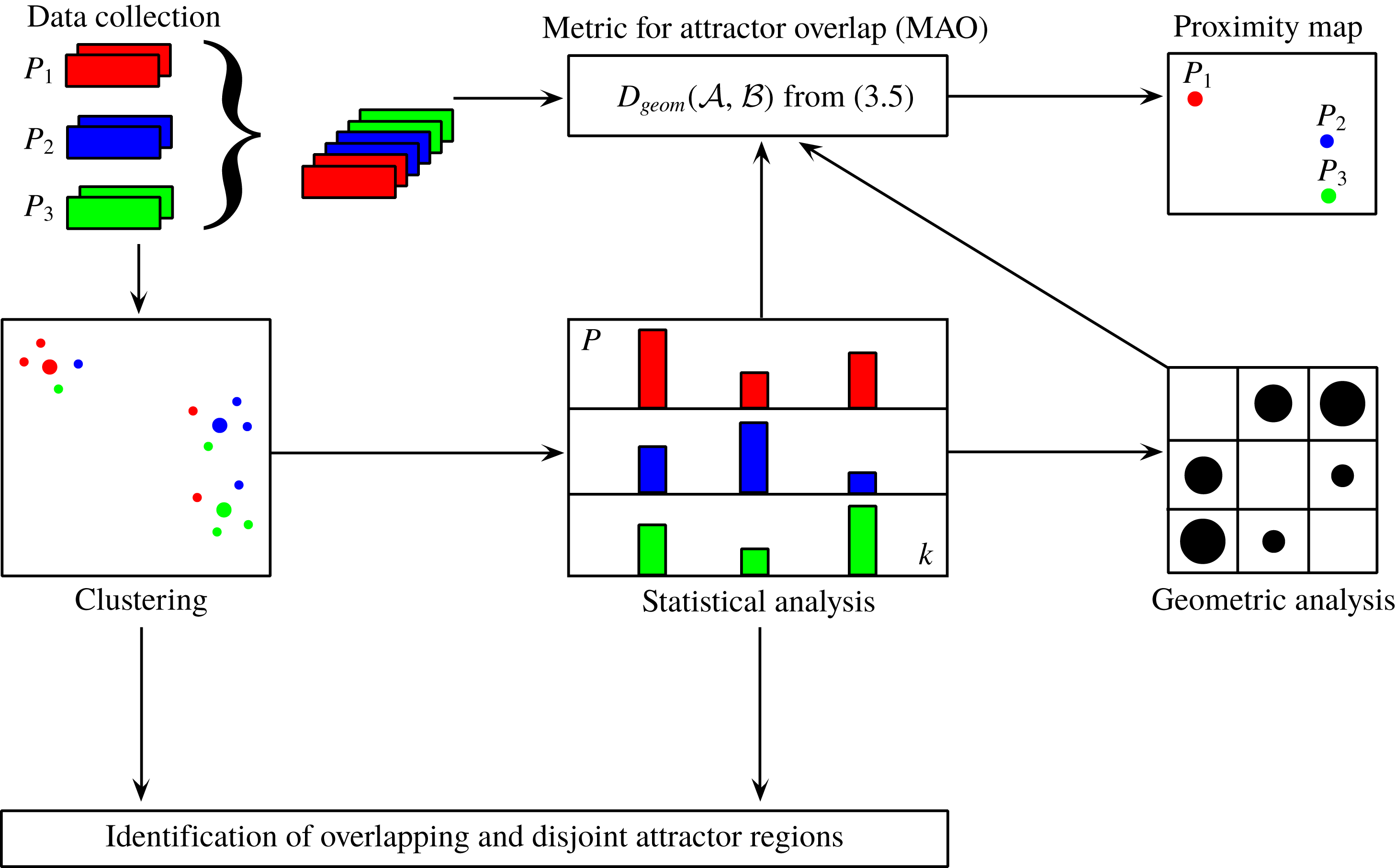
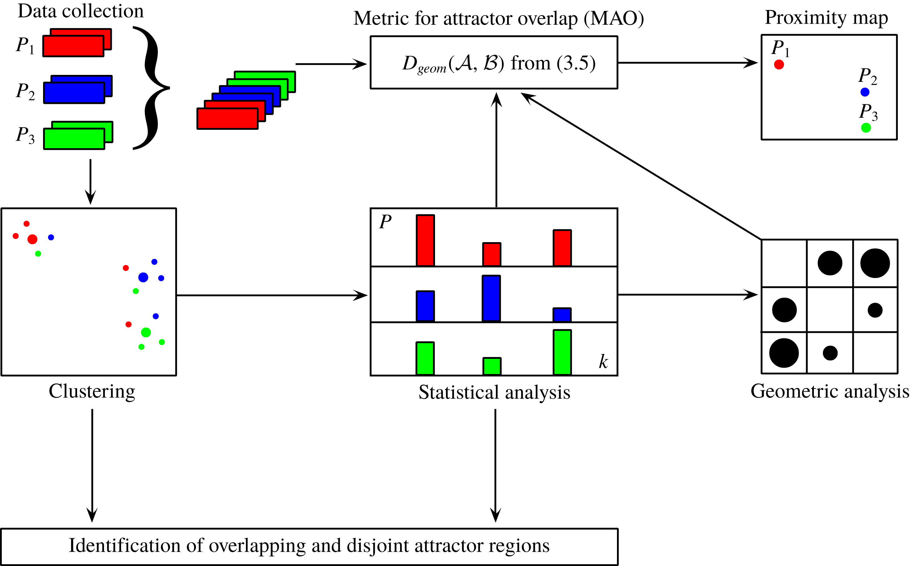
Figure 1 previews the proposed methodology. The top row illustrates the processing from the raw data of multiple attractors (left) to the proximity map (right) employing the snapshot MAO. The centre row represents the coarse-grained version with clustering. Clustering opens the opportunity to pinpoint the overlap region of attractors to a few select velocity fields, i.e. shared centroids, as indicated in the bottom row.
Schematic of the pipeline for the metric of attractor overlap and associated proximity maps. Here,
 $P_{1}$
,
 $P_{2}$
and
 $P_{3}$
refer to data sets outlined in § 3, i.e. sets of snapshots which are statistically representative of an attractor under a given operating condition. Of course, the number of data sets is typically much larger.
 $D$
is the metric of attractor overlap (§ 2.1). Its two arguments
 $P$
,
 $Q$
represent data sets, like
 $P_{1}$
,
 $P_{2}$
and
 $P_{3}$
. The proximity map (top right) is explained in § 2.3. The coarse graining by clusters (centre row) is discussed in § 2.4 and the identification of overlapping and disjoint attractor regions (bottom row) is outlined in § 2.5.
2.1 Metric of attractor overlap for snapshot data
Let
 $\boldsymbol{u}(\boldsymbol{x})$
and
 $\boldsymbol{v}(\boldsymbol{x})$
be two velocity fields in the domain
 $\unicode[STIX]{x1D6FA}$
. We define the distance between these fields as
 $$\begin{eqnarray}D(\boldsymbol{u},\boldsymbol{v})=\sqrt{\int _{\unicode[STIX]{x1D6FA}}\,\text{d}\boldsymbol{ x}\Vert \boldsymbol{u}(\boldsymbol{x})-\boldsymbol{ v}(\boldsymbol{x})\Vert ^{2}}.\end{eqnarray}$$
Here,
 $\Vert \cdot \Vert$
denotes the Euclidean norm. Note that this distance is based on the norm associated with the Hilbert space
 ${\mathcal{L}}^{2}(\unicode[STIX]{x1D6FA})$
of square-integrable functions. It fulfils all properties of a metric, like positive definiteness, commutativity and triangle inequality. For the fluidic pinball data of § 3.1, the distance measure uses the whole computational domain
 $\unicode[STIX]{x1D6FA}$
. For the turbulent boundary layer of § 3.2, a subdomain over the whole actuated surface is chosen. The surface actuation leads to a small domain deformation. This deformation is neglected and the operations are performed in a stationary domain in which the grid points assume their unactuated equilibrium location.
In this section, we define a measure for the attractor similarity based on the snapshot configuration and the Hilbert-space metric. Loosely speaking, the difference between two attractors
 ${\mathcal{A}}$
and
 ${\mathcal{B}}$
– represented by their snapshot ensembles – is geometrically defined as the sum of the average distances between the snapshots of
 ${\mathcal{A}}$
to
 ${\mathcal{B}}$
and vice versa.
In the following, this quantity is defined. For simplicity, let us consider two attractors
 ${\mathcal{A}}$
and
 ${\mathcal{B}}$
. Let
 ${\mathcal{M}}:=\{\boldsymbol{u}^{m}\}_{m=1}^{M}$
be the union of all snapshots from both attractors. For simplicity, we assume the generic case that all snapshots are pairwise different. The subset of
 ${\mathcal{M}}$
belonging to attractor
 ${\mathcal{A}}$
is defined by the characteristic function
 $$\begin{eqnarray}\unicode[STIX]{x1D712}_{{\mathcal{A}}}^{m}:=\left\{\begin{array}{@{}ll@{}}1,\quad & \text{if }\boldsymbol{u}^{m}\in {\mathcal{A}},\\ 0,\quad & \text{otherwise}.\end{array}\right.\end{eqnarray}$$
The number of snapshots in
 ${\mathcal{A}}$
is given by
 $M_{A}:=\sum _{m=1}^{M}\unicode[STIX]{x1D712}_{{\mathcal{A}}}^{m}$
. Similar formulae hold for attractor
 ${\mathcal{B}}$
.
The distance of a snapshot
 $\boldsymbol{u}$
to
 ${\mathcal{B}}$
is defined by the closest corresponding snapshot of
 ${\mathcal{B}}$
,
 $$\begin{eqnarray}D(\boldsymbol{u},{\mathcal{B}})=\min _{\substack{ m=1,\ldots ,M \\ \unicode[STIX]{x1D712}_{{\mathcal{B}}}^{m}=1}}D(\boldsymbol{u},\boldsymbol{u}^{m}).\end{eqnarray}$$
The average distance of attractor
 ${\mathcal{A}}$
to
 ${\mathcal{B}}$
is defined by
 $$\begin{eqnarray}D({\mathcal{A}},{\mathcal{B}})=\frac{1}{M_{A}}\mathop{\sum }_{\substack{ m=1,\ldots ,M \\ \unicode[STIX]{x1D712}_{{\mathcal{A}}}^{m}=1}}D(\boldsymbol{u}^{m},{\mathcal{B}}).\end{eqnarray}$$
This distance is not commutative. Suppose
 ${\mathcal{A}}$
has only one snapshot of
 ${\mathcal{B}}$
and
 ${\mathcal{B}}$
has many more elements. In this case,
 $D({\mathcal{A}},{\mathcal{B}})=0$
but
 $D({\mathcal{B}},{\mathcal{A}})>0$
. Hence, we define a symmetrized version of this distance
 $$\begin{eqnarray}D_{geom}({\mathcal{A}},{\mathcal{B}}):=\frac{D({\mathcal{A}},{\mathcal{B}})+D({\mathcal{B}},{\mathcal{A}})}{2}.\end{eqnarray}$$
We refer to this quantity as the metric of attractor overlap (MAO). MAO has the properties of a metric for snapshot ensembles
 ${\mathcal{A}}$
and
 ${\mathcal{B}}$
and
 ${\mathcal{C}}$
since the defining properties can be shown for the generic case of pairwise different snapshots.
(i) Positive definiteness:
 $D_{geom}({\mathcal{A}},{\mathcal{B}})\geqslant 0$
for all
${\mathcal{A}},{\mathcal{B}}$
and (2.6)$$\begin{eqnarray}{\mathcal{A}}={\mathcal{B}}\quad \Leftrightarrow \quad D_{geom}({\mathcal{A}},{\mathcal{B}})=0.\end{eqnarray}$$
(ii) Symmetry: by definition (2.5),
(2.7)$$\begin{eqnarray}D_{geom}({\mathcal{A}},{\mathcal{B}})=D_{geom}({\mathcal{B}},{\mathcal{A}}).\end{eqnarray}$$
(iii) Triangle inequality:
(2.8)$$\begin{eqnarray}D_{geom}({\mathcal{A}},{\mathcal{C}})\leqslant D_{geom}({\mathcal{A}},{\mathcal{B}})+D_{geom}({\mathcal{B}},{\mathcal{C}}).\end{eqnarray}$$



To illustrate the physical implications of MAO, we consider several cases. If
 ${\mathcal{A}}$
and
 ${\mathcal{B}}$
only consist of velocity fields
 $\boldsymbol{u}$
and
 $\boldsymbol{v}$
, respectively, their distance coincides with the Hilbert-space metric,
 $D({\mathcal{A}},{\mathcal{B}})=D(\boldsymbol{u},\boldsymbol{v})$
.
Let
 ${\mathcal{A}}$
contain one velocity field, e.g. an unstable steady solution, and
 ${\mathcal{B}}$
contains many fields, e.g. snapshots of a stable periodic dynamics. Then
 $D({\mathcal{A}},{\mathcal{B}})$
is the smallest distance between the steady solution and the snapshots on limit cycle, while
 $D({\mathcal{B}},{\mathcal{A}})$
represents the average distance between fixed point and limit cycle. This asymmetry makes sense;
 $D({\mathcal{A}},{\mathcal{B}})$
quantifies how well elements of
 ${\mathcal{A}}$
can be represented by elements of
 ${\mathcal{B}}$
on average. This measure is inherently non-commutative: a small set may be better represented by a rich set than the other way around. MAO is the average of both, i.e. an effective average distance between two attractors, not the minimal geometric distance between the closest elements of two sets.
Next, let us assume that both attractors arise from periodic dynamics defining limit cycles with the same origin and the same plane but with radii 10 and 11. In this case, the distance approaches unity for sufficiently large number of snapshots. Complete attractor overlap,
 $D_{geom}({\mathcal{A}},{\mathcal{B}})=0$
, implies that
 ${\mathcal{A}}$
and
 ${\mathcal{B}}$
have the same snapshots. The probability of their occurrence may differ in both data.
In summary, MAO averages how well each snapshot of
 ${\mathcal{A}}$
is represented by the closest snapshot of
 ${\mathcal{B}}$
and vice versa. Note that some of the above statements need to be refined in case of identical snapshots. We shall not pause to do so.
2.2 Generalization of MAO to continuous data
Intuitively, the metric can be expected to converge against a continuous ensemble-averaged value for infinite number of snapshots
 $M$
. Here, we generalize the above metric for continuous data. This generalization highlights geometric and statistical implications of the metric.
For simplicity, we restrict the discussion to
 $N$
-dimensional vectors
 $\boldsymbol{a}\in R^{N}$
, e.g. the first POD mode coefficients. Let
 $\unicode[STIX]{x1D70C}_{{\mathcal{A}}}(\boldsymbol{a})$
and
 $\unicode[STIX]{x1D70C}_{{\mathcal{B}}}(\boldsymbol{a})$
denote the probability distributions for
 $\boldsymbol{a}\in R^{N}$
of attractors
 ${\mathcal{A}}$
and
 ${\mathcal{B}}$
, respectively. In the following, the attractor symbol will be used also for the set of its points.
In analogy to (2.3), the distance of the vector
 $\boldsymbol{a}\in {\mathcal{A}}$
to the attractor
 ${\mathcal{B}}$
is defined by the infimum of the corresponding distances,
 $$\begin{eqnarray}D(\boldsymbol{a},{\mathcal{B}})=\inf _{\boldsymbol{b}\in {\mathcal{B}}}D(\boldsymbol{a},\boldsymbol{b}).\end{eqnarray}$$
Following (2.4), the distance of attractor
 ${\mathcal{A}}$
to attractor
 ${\mathcal{B}}$
is defined as the average distance of the
 ${\mathcal{A}}$
elements to
 ${\mathcal{B}}$
,
 $$\begin{eqnarray}D({\mathcal{A}},{\mathcal{B}})=\int \,\text{d}\boldsymbol{a}\unicode[STIX]{x1D70C}_{{\mathcal{A}}}(\boldsymbol{a})D(\boldsymbol{a},{\mathcal{B}}).\end{eqnarray}$$
The symmetrization (2.5) completes the definition of the metric. In principle, the distance can more generally be formulated in terms of Borel probability measures on
 $L^{2}(\unicode[STIX]{x1D6FA})$
.
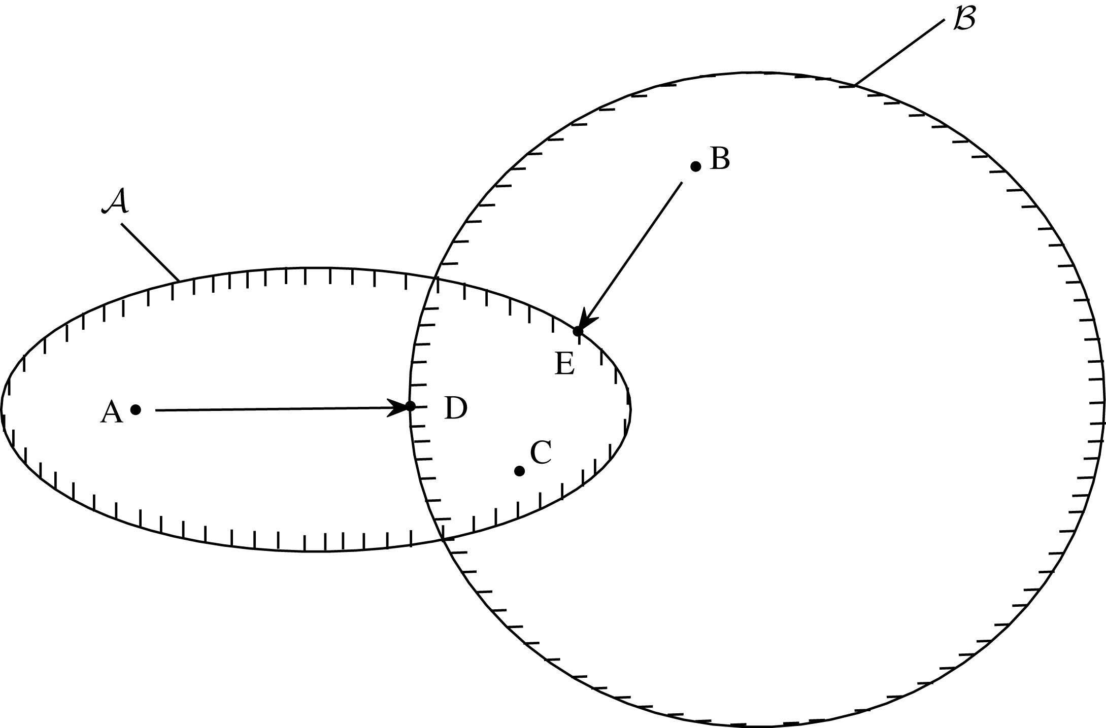
Schematic of the metric of attractor overlap for continuous data.

Figure 2 illustrates the definition. The attractor sets are the support of the probability density, for instance
 $\boldsymbol{a}\in {\mathcal{A}}\Leftrightarrow \unicode[STIX]{x1D70C}(\boldsymbol{a})\not =0$
. Only the disjoint sets
 ${\mathcal{A}}\backslash {\mathcal{B}}$
and
 ${\mathcal{B}}\backslash {\mathcal{A}}$
contribute to the metric. The closest neighbour
 $D\in {\mathcal{B}}$
to
 $A\in {\mathcal{A}}\backslash {\mathcal{B}}$
defines the distance
 $D(A,{\mathcal{B}})$
. Similarly,
 $B\in {\mathcal{B}}\backslash {\mathcal{A}}$
is best represented by point
 $E\in {\mathcal{A}}$
. MAO averages these distances. The intersection of both sets does not contribute to the metric. For instance,
 $C\in {\mathcal{A}}\bigcap {\mathcal{B}}$
has, by definition, vanishing distance to both sets. This implies a vanishing metric for attractors with the same support
 ${\mathcal{A}}={\mathcal{B}}$
. As a technical issue, the existence of points
 $D$
and
 $E$
assumes compact attractor sets. Otherwise,
 $D$
and
 $E$
are the limiting points at the border of the attractor sets.
It should be noted that complete mutual attractor overlap implies identical characteristic functions
 $\unicode[STIX]{x1D712}_{{\mathcal{A}}}(\boldsymbol{a})=\unicode[STIX]{x1D712}_{{\mathcal{B}}}(\boldsymbol{b})$
. In other words,
 $\unicode[STIX]{x1D70C}_{{\mathcal{A}}}(\boldsymbol{a})=0\Leftrightarrow \unicode[STIX]{x1D70C}_{{\mathcal{B}}}(\boldsymbol{a})=0$
. However,
 ${\mathcal{A}}={\mathcal{B}}$
does not imply
 $\unicode[STIX]{x1D70C}_{{\mathcal{A}}}(\boldsymbol{a})=\unicode[STIX]{x1D70C}_{{\mathcal{B}}}(\boldsymbol{a})\not =0$
. Two attractors can share the same points, i.e. have a vanishing MAO, but have different probability distributions. Statistical similarity and geometrical closeness are two fundamentally different concepts. Consider two close points with different probability densities. From a geometric point of view, only the distance is relevant. From a statistical perspective, the resulting differences in first and higher moments are of interest.
The metric between the two attractors has similarity with the Hausdorff distance between two sets. The Hausdorff distance distils the worst-case scenario or rare extreme events, i.e. the maximum distance between a point of one set and its closest neighbour of the other set. For instance, the points from two slightly different Gaussian distributions have arbitrarily large Hausdorff distance for increasing number of points. In contrast, MAO quantifies the average distance which can be considered more representative for attractor data.
2.3 Proximity map
In the case of two attractors
 ${\mathcal{A}}$
and
 ${\mathcal{B}}$
, the closeness can be characterized by MAO, i.e. a single number. The comparison of many attractors
 ${\mathcal{A}}^{l},l=1,\ldots ,L$
with
 $L\gg 1$
is more challenging. In this case, the complete snapshot set
 $\{\boldsymbol{u}^{m}\}_{m=1}^{M}$
comprises the elements of all
 $L$
attractors. The closeness of the attractors
 ${\mathcal{A}}^{l}$
may be visualized in a two-dimensional proximity map which preserves the metric of attractor overlap as well as possible (see figure 1 top, right). This task is performed by multi-dimensional scaling (Cox & Cox Reference Cox and Cox2000) presented in the following.
The relative distances between the attractors is expressed by the symmetric matrix
 $$\begin{eqnarray}D_{ln}:=D_{geom}({\mathcal{A}}^{l},{\mathcal{A}}^{n}),\quad l,n=1,\ldots ,L.\end{eqnarray}$$
Let
 $\unicode[STIX]{x1D738}^{l}\in \mathbb{R}^{2}$
be a two-dimensional feature vector associated with the
 $l$
th operating condition. The goal of a proximity map is to find a mapping
 ${\mathcal{A}}\mapsto \unicode[STIX]{x1D738}$
such that the pointwise distances in the feature plane are preserved as well as possible,
 $$\begin{eqnarray}\mathop{\sum }_{l,n=1}^{L}(D_{ln}-\Vert \unicode[STIX]{x1D738}^{l}-\unicode[STIX]{x1D738}^{n}\Vert )^{2}\overset{!}{=}\text{min}.\end{eqnarray}$$
At this point, the feature plane is indeterminate with respect to translation, rotation and reflection. However, one can request that the centre of the feature vector is at the origin, removing the translative degree of freedom. Moreover, the variances of the first feature coordinate can be maximized, removing the rotational degree of freedom. Now, only the indeterminacy with respect to reflection is left, as for POD modes.
The proximity map can easily be generalized for higher-dimensional feature spaces. Moreover, the proximity map requires only a distance matrix and can thus also be used for snapshots using the snapshot metric (2.1). Proximity maps have been presented for mixing layer and Ahmed body wake data (Kaiser et al. Reference Kaiser, Noack, Cordier, Spohn, Segond, Abel, Daviller, Östh, Krajnović and Niven2014) and for ensembles of control laws (Duriez, Brunton & Noack Reference Duriez, Brunton and Noack2016; Kaiser, Li & Noack Reference Kaiser, Li and Noack2017a ; Kaiser et al. Reference Kaiser, Noack, Spohn, Cattafesta and Morzyński2017b ).
2.4 Cluster analysis
Next, the
 $M$
snapshots
 $\boldsymbol{u}^{m}(\boldsymbol{x})$
,
 $m=1,\ldots ,M$
, are coarse grained into
 $K$
representative centroids
 $\boldsymbol{c}_{k}(\boldsymbol{x})$
,
 $k=1,\ldots ,K$
. These centroids are chosen to minimize the total variance of the snapshots
 $\boldsymbol{u}^{m}$
with respect to the nearest centroid
 $\boldsymbol{c}_{k}$
,
 $$\begin{eqnarray}V=\mathop{\sum }_{k=1}^{K}\mathop{\sum }_{\boldsymbol{u}^{m}\in {\mathcal{C}}_{k}}D^{2}(\boldsymbol{u}^{m},\boldsymbol{c}_{k})\overset{!}{=}\text{min}.\end{eqnarray}$$
Each centroid
 $\boldsymbol{c}_{k}$
defines a cluster
 ${\mathcal{C}}_{k}$
containing all flow states
 $\boldsymbol{u}^{m}$
which are closer to
 $\boldsymbol{c}_{k}$
as compared to any other centroid
 $\boldsymbol{c}_{j}$
,
 $j\not =k$
. Thus, each snapshot
 $\boldsymbol{u}^{m}$
can be attributed to one cluster
 ${\mathcal{C}}_{k}$
. This cluster affiliation is coded as characteristic function
 $$\begin{eqnarray}T_{k}^{m}:=\left\{\begin{array}{@{}ll@{}}1,\quad & \text{if }\boldsymbol{u}^{m}\in {\mathcal{C}}_{k},\\ 0,\quad & \text{otherwise}.\end{array}\right.\end{eqnarray}$$
The number of snapshots in the
 $k$
th cluster reads
 $$\begin{eqnarray}N_{k}=\mathop{\sum }_{m=1}^{M}\,T_{k}^{m}.\end{eqnarray}$$
The centroids can also be expressed in terms of this characteristic function. It can be shown that they are the mean of all snapshots in the corresponding cluster,
 $$\begin{eqnarray}\boldsymbol{c}_{k}=\frac{1}{N_{k}}\mathop{\sum }_{\boldsymbol{u}^{m}\in {\mathcal{C}}_{k}}\boldsymbol{u}^{m}=\frac{1}{N_{k}}\mathop{\sum }_{m=1}^{M}T_{k}^{m}\boldsymbol{u}^{m}.\end{eqnarray}$$
Numerically, the optimization problem (2.13) for the centroids is solved using k-means clustering (Steinhaus Reference Steinhaus1956; MacQueen Reference MacQueen1967; Lloyd Reference Lloyd1982) and k-means
 $++$
(Arthur & Vassilvitskii Reference Arthur and Vassilvitskii2007) for the initialization. Since k-means shows a dependence on the initial conditions, we run the corresponding MATLAB routine for 1000 initial conditions and select the one having the smallest variance. The iteration stops when convergence is reached, i.e. the characteristic function (2.14) does not change. The number of iterations is limited to 10 000 iterations.
In principle, k-means clustering can lead to two different coarse grainings with the same resolution level. For instance, the centroids of 10 clusters of a uniformly populated circle may be at angles
 $0^{\circ },36^{\circ },\ldots ,324^{\circ }$
or at angles
 $18^{\circ },54^{\circ },\ldots ,342^{\circ }$
. In practice, this typically implies a rare symmetry, like a rotation invariant uniformly populated data set in our example. Second, the difference between the centroids vanishes with increasing number of clusters. Third, only one set of centroids is used for the comparison leading to comparable discretization errors.
For practical reasons, we perform a lossless POD decomposition prior to the clustering of
 $M$
snapshots into the mean flow
 $\boldsymbol{u}_{0}$
and
 $M-1$
modes
 $\boldsymbol{u}_{i}$
,
 $i=1,\ldots ,M-1$
(see appendix A). Let
 $\boldsymbol{u}=\boldsymbol{u}_{0}+\sum _{m=1}^{M-1}a_{i}\boldsymbol{u}_{i}$
be one snapshot and
 $\boldsymbol{v}=\boldsymbol{u}_{0}+\sum _{m=1}^{M-1}b_{i}\boldsymbol{u}_{i}$
another one. Then,
 $D^{2}(\boldsymbol{u},\boldsymbol{v})=\sum _{m=1}^{M-1}(a_{i}-b_{i})^{2}$
. The right-hand side requires
 $3M$
floating point operations while the computational load of the integral (2.1) scales with the number of grid points and is much larger even for the employed grids. It should be noted that these immense computational savings are enabled by an expensive computation of POD modes. However, for the fluidic pinball data, the POD correlation matrix comprises approximately 24.5 million space integrals while the employed k-means
 $++$
with 1000 initial conditions with up to 10 000 iterations requires up to 70 billion (!) integrals, i.e. three orders of magnitudes more. The savings for the turbulent boundary layer are comparable.
The clustering enables to characterize each operating condition by a corresponding probability distribution. Let
 $l=1,\ldots ,L$
be the index of the
 $L$
operating conditions. Let
 $N_{k}^{l}$
be the number of snapshots of the
 $l$
th attractor data in the
 $k$
th cluster. Let
 $N^{l}=\sum _{k=1}^{K}N_{k}^{l}$
be the total number of snapshots of the
 $l$
th attractor data. Then, the probability that a snapshot belonging to the
 $l$
th operating condition lies in the
 $k$
th cluster reads
 $$\begin{eqnarray}P_{k}^{l}=\frac{N_{k}^{l}}{N^{l}},\quad k=1,\ldots ,K.\end{eqnarray}$$
In particular, the probability distribution is determined here as relative frequencies of cluster visits and fulfils the non-negativity,
 $P_{k}^{l}\geqslant 0$
, and normalization condition,
 $\sum _{k=1}^{K}P_{k}^{l}=1$
.
2.5 Cluster-based analysis of the attractor overlap and dissimilarity
In this section, we define a measure for the attractor similarity based on the centroid configuration. Each snapshot
 $\boldsymbol{u}^{m}$
is represented by its closest centroid
 $\boldsymbol{c}_{k}$
. Let
 ${\mathcal{A}}$
and
 ${\mathcal{B}}$
be two sets of attractor data, say
 ${\mathcal{A}}^{l}$
and
 ${\mathcal{A}}^{n}$
,
 $l,n\in \{1,\ldots ,L\}$
. Let
 $\boldsymbol{P}=(P_{1}^{l},\ldots ,P_{K}^{l})$
and
 $\boldsymbol{Q}=(P_{1}^{n},\ldots ,P_{K}^{n})$
be the corresponding cluster-based probability distributions. The snapshot-based metric is coarse grained to the average distance between the centroids of attractor
 ${\mathcal{A}}$
and
 ${\mathcal{B}}$
,
 $$\begin{eqnarray}D_{geom}(\boldsymbol{P},\boldsymbol{Q})=\frac{1}{2}\mathop{\sum }_{k=1}^{K}[P_{k}^{l}D(\boldsymbol{c}_{k},{\mathcal{B}}^{c})+P_{k}^{n}D(\boldsymbol{c}_{k},{\mathcal{A}}^{c})].\end{eqnarray}$$
Here
 ${\mathcal{A}}^{c}$
and
 ${\mathcal{B}}^{c}$
denote the centroid ensembles associated with attractors
 ${\mathcal{A}}$
and
 ${\mathcal{B}}$
, respectively. This formula can be derived from (2.5) replacing the snapshots
 $\boldsymbol{u}^{m}$
by the closest centroids
 $\boldsymbol{c}_{k}$
and taking into account the population size. The centre row of figure 1 illustrates the approximative cluster-based analysis. Evidently, (2.18) is an approximation of (2.5) and is equivalent for the maximum cluster resolution
 $K=M$
of snapshots. In this case, each snapshot represents a centroid and the probability distributions associated with each cluster are unit vectors.
The main computational load for MAO comes from the distance matrix of the snapshots or centroids. The computational savings of the cluster-based measure (2.18) with respect to snapshot-based metric (2.5) scale with
 $(K/M)^{2}$
. For the fluidic pinball study with
 $M=3500$
snapshots and
 $K=50$
clusters, this translates to the quite dramatic factor of
 ${\approx}2/10\,000$
. This saving does not include the operations for clustering. These can be large for a field-based clustering of § 2.4 and small for an alternative clustering, e.g. based on few aerodynamic force components.
A lossless POD reduces the computational load of the distance matrix and of the clustering to a tiny fraction of the original cost. The main cost of POD originates from the correlation matrix which requires a similar amount of operations as the distance matrix. The advantage of POD preprocessing is the many post-processing options at negligible cost.
As a side note, a commonly used metric for probability distributions is the Jensen–Shannon distance (see appendix B). This distance measures probability differences on shared clusters but is blind to the geometric distances of disjoint clusters. In the previous example of concentric co-planar circles, the metric is the same for all non-identical radii.
3 Plant configurations
The comparison methodology MAO is applied to two configurations with many data sets from open-loop actuation studies. A two-dimensional fluidic pinball configuration (§ 3.1) is computationally inexpensive and allows an extensive visualization of the flow quantities while exhibiting a complex behaviour. The open-loop drag reduction of a three-dimensional turbulent boundary layer (§ 3.2) constitutes the second example. The corresponding data allow us to assess MAO for a complex three-dimensional flow with a large range of scales and frequencies.
3.1 Fluidic pinball simulation
In this section, the computation of the employed flow data is described. In § 3.1.1, the configuration of the fluidic pinball is introduced. The corresponding direct Navier–Stokes solver is described in § 3.1.2. Finally, the fluidic pinball simulation of seven open-loop actuations is detailed. These flow data are subjected to the proposed comparison methodology of the next section.
3.1.1 Fluidic pinball configuration
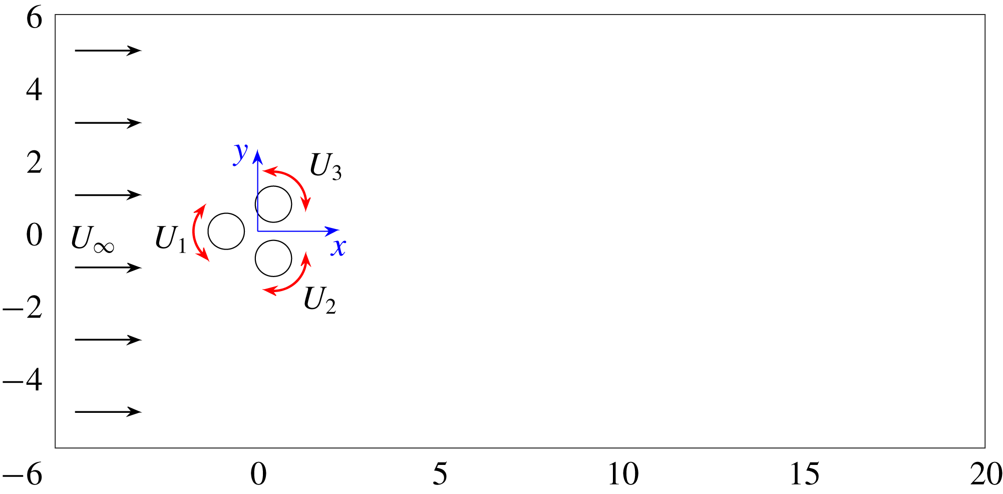
In the following, the considered two-dimensional flow control configuration is described. Three equal circular cylinders with radius
 $R$
are placed parallel to each other in a viscous incompressible uniform flow at speed
 $U_{\infty }$
(see figure 3). The centres of the cylinders form an equilateral triangle with side length
 $3R$
, symmetrically positioned with respect to the flow. The leftmost triangle vertex points upstream, while the rightmost side is orthogonal to the oncoming flow. Thus, the transverse extent of the three-cylinder configuration is given by
 $5R$
.
Configuration of the fluidic pinball. The Cartesian coordinate system
 $(x,y)$
is depicted at the centre of the cylinders.

This flow is described in a Cartesian coordinate system where the
 $x$
-axis points in the direction of the flow, the
 $z$
-axis is aligned with the cylinder axes and the
 $y$
-axis is orthogonal to both (see figure 3). The origin
 $\mathbf{0}$
of this coordinate system coincides with the geometric centre of the cylinder triangle. The location is denoted by
 $\boldsymbol{x}=(x,y,z)=x\boldsymbol{e}_{x}+y\boldsymbol{e}_{y}+z\boldsymbol{e}_{z}$
, where
 $\boldsymbol{e}_{x,y,z}$
are unit vectors pointing in the direction of the corresponding axes. Analogously, the velocity reads
 $\boldsymbol{u}=(u,v,w)=u\boldsymbol{e}_{x}+v\boldsymbol{e}_{y}+w\boldsymbol{e}_{z}$
. The pressure is denoted by
 $p$
and the time by
 $t$
. In the following, we assume a two-dimensional flow, i.e. no dependence of any flow quantity on
 $z$
and vanishing spanwise velocity
 $w\equiv 0$
.
The Newtonian fluid is characterized by a constant density
 $\unicode[STIX]{x1D70C}$
and kinematic viscosity
 $\unicode[STIX]{x1D708}$
. In the following, all quantities are assumed to be non-dimensionalized with cylinder diameter
 $D=2R$
, the velocity
 $U_{\infty }$
and the fluid density
 $\unicode[STIX]{x1D70C}$
. The corresponding Reynolds number is
 $Re_{D}=100$
where
 $Re_{D}=U_{\infty }D/\unicode[STIX]{x1D708}$
. The Reynolds number based on the transverse length
 $L=5D$
is 2.5 times larger. The non-dimensionalization with respect to the diameter is more common for clusters of cylinders (Hu & Zhou Reference Hu and Zhou2008a
,Reference Hu and Zhou
b
; Bansal & Yarusevych Reference Bansal and Yarusevych2017) and will be adopted in the following. With this non-dimensionalization, the cylinder axes are located at
 $$\begin{eqnarray}\left.\begin{array}{@{}c@{}}x_{F}=-\sqrt{3}/2,\quad y_{F}=0,\\ x_{B}=\sqrt{3}/4,\quad y_{B}=-3/4,\\ x_{T}=\sqrt{3}/4,\quad y_{T}=+3/4.\end{array}\right\}\end{eqnarray}$$
Here, and in the following, the subscripts ‘
 $F$
’, ‘
 $B$
’ and ‘
 $T$
’ refer to the front, bottom and top cylinders. An alternate reference is the subscripts 1, 2, 3 for the front, bottom and top cylinders, respectively.
The incompressibility condition reads
 $$\begin{eqnarray}\unicode[STIX]{x1D735}\boldsymbol{\cdot }\boldsymbol{u}=0,\end{eqnarray}$$
where
 $\unicode[STIX]{x1D735}$
represents the Nabla operator. The evolution is described by the Navier–Stokes equations,
 $$\begin{eqnarray}\unicode[STIX]{x2202}_{t}\boldsymbol{u}+\unicode[STIX]{x1D735}\boldsymbol{\cdot }(\boldsymbol{u}\otimes \boldsymbol{u})=-\unicode[STIX]{x1D735}p+\frac{1}{Re_{D}}\triangle \boldsymbol{u},\end{eqnarray}$$
where
 $\unicode[STIX]{x2202}_{t}$
and
 $\triangle$
denote the partial derivative with respect to time
 $t$
and the Laplace operator, respectively. The dot ‘
 $\cdot$
’ and dyadic product sign ‘
 $\otimes$
’ refer to inner and outer tensor products.
Without forcing, the boundary conditions comprise a no-slip condition on the cylinder and a free-stream condition in the far field,
 $$\begin{eqnarray}\boldsymbol{u}=\mathbf{0}\text{ on the cylinder and }\boldsymbol{u}=\boldsymbol{e}_{x}\text{ at infinity.}\end{eqnarray}$$
As initial condition, we chose the unstable steady Navier–Stokes solution
 $\boldsymbol{u}_{s}(\boldsymbol{x})$
. This solution is computed with a Newton search algorithm, as in (Noack et al.
Reference Noack, Afanasiev, Morzyński, Tadmor and Thiele2003). Vortex shedding is kick-started with cylinder rotations in the first period.
The forcing is exerted by rotation of the cylinders with circumferential velocities
 $b_{1}=U_{1}=U_{F}$
,
 $b_{2}=U_{2}=U_{B}$
and
 $b_{3}=U_{3}=U_{T}$
for the front, bottom and top cylinders, respectively. The actuation command
 $\boldsymbol{b}=(b_{1},b_{2},b_{3})=(U_{1},U_{2},U_{3})$
is preferably used for control theory purposes (Brunton & Noack Reference Brunton and Noack2015; Duriez et al.
Reference Duriez, Brunton and Noack2016) while
 $(U_{F},U_{B},U_{T})$
are more natural for a discussion of physical mechanisms. The actuation is conveniently expressed with the vector cross-product ‘
 $\times$
’,
 $$\begin{eqnarray}\boldsymbol{u}=2U_{i}(\boldsymbol{x}-\boldsymbol{x}_{i})\times \boldsymbol{e}_{z}\quad \text{on the }i\text{th cylinder},\end{eqnarray}$$
where
 $\boldsymbol{x}_{i}$
denotes the centre of the
 $i$
th cylinder.
The factor 2 counterbalances the non-dimensional radius
 $1/2$
.
We like to refer to this configuration as the fluidic pinball as the rotation speeds allow one to change the paths of the incoming fluid particles like flippers manipulate the ball of a conventional pinball machine. The front cylinder rotation may determine if the fluid particle passes by on the upper or lower side of the cylinder, while the top and bottom cylinder may guide the particle through the interior.
3.1.2 Direct Navier–Stokes solver
The chosen computational domain is bounded by the rectangle
 $[-6,20]\times [-6,6]$
and excludes the interior of the cylinders
 $$\begin{eqnarray}\unicode[STIX]{x1D6FA}=\{(x,y):-6\leqslant x\leqslant 20\wedge |y|\leqslant 6\wedge (x-x_{i})^{2}+(y-y_{i})^{2}\geqslant 1/4,i=1,2,3\}.\end{eqnarray}$$
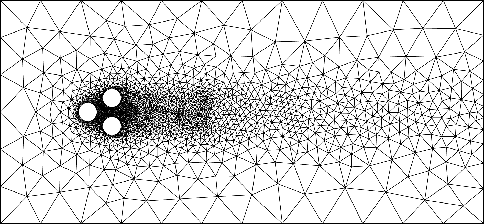
This flow domain is discretized on an unstructured grid with 4225 triangles and 8633 vertices (see figure 4). This discretization optimizes the speed of the numerical simulation while keeping the accuracy at an acceptable level. Increasing the number of triangles by a factor 4 yields virtually indistinguishable results. The Navier–Stokes equation is numerically integrated with an implicit finite-element method (Noack et al.
Reference Noack, Afanasiev, Morzyński, Tadmor and Thiele2003, Reference Noack, Stankiewicz, Morzyński and Schmid2016). The numerical integration is second-order accurate in space and third-order accurate in time. This direct numerical simulation has a companion experiment at turbulent Reynolds numbers
 $Re_{D}\approx 4000{-}6000$
(Raibaudo et al.
Reference Raibaudo, Zhong, Martinuzzi and Noack2017).
Grid of the fluidic pinball simulation.

3.1.3 Attractor data
We simulate seven actuations in a single simulation starting at
 $t=0$
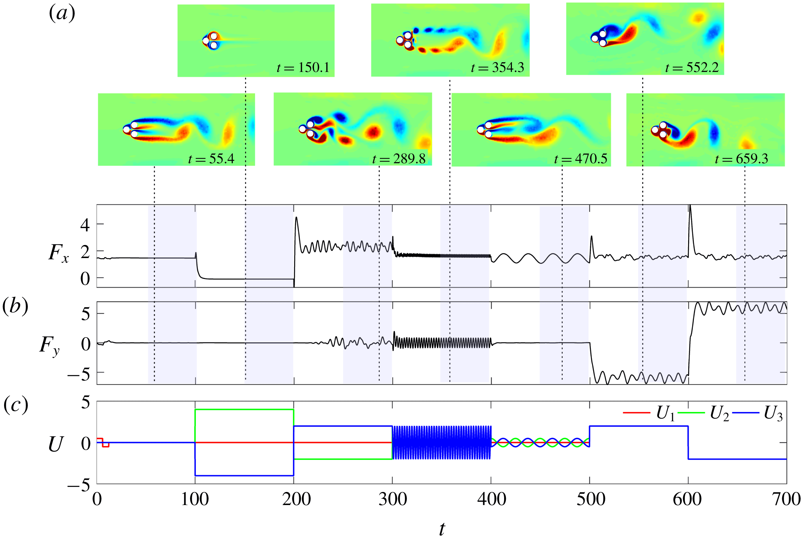
with the unstable steady Navier–Stokes solution. Each phase is associated with one control law and lasts 100 convective time units based on the diameter of one cylinder, i.e. according to the performed non-dimensionalization. Figure 5 provides a preview of the simulation which is detailed in the following.
Operating conditions of the fluidic pinball simulation. (c) Time series of the actuation commands for each cylinder over all phases together. (a) The flow of each phase is illustrated with a vorticity snapshot corresponding to maximum lift or minimum drag of the converged phase. (b) The time series of the total drag
 $F_{x}$
and total lift
 $F_{y}$
are displayed.

In the first phase, vortex shedding is kick-started with a motion of the front cylinder,
 $$\begin{eqnarray}\displaystyle U_{F} & = & \displaystyle \left\{\begin{array}{@{}ll@{}}1/2,\quad & t\leqslant 6.25,\\ -1/2,\quad & 6.25<t\leqslant 12.5,\\ 0,\quad & \text{otherwise}\end{array}\right.\end{eqnarray}$$
 $$\begin{eqnarray}\displaystyle U_{B} & = & \displaystyle -U_{T}=0.\end{eqnarray}$$
 $12.5$
corresponds to a Strouhal number of
 $0.2$
based on the transverse width
 $5R$
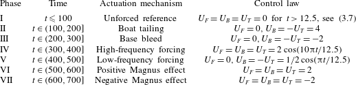
. Without this kick-start, the onset of vortex shedding may require hundreds of shedding periods depending on accuracy of the steady solution and the truncation errors in the Navier–Stokes solver. In the second phase, strong boat tailing with symmetric cylinder rotation of the upper and lower cylinders pushes the separation close to the
 $x$
-axis and completely suppresses vortex shedding,
 $$\begin{eqnarray}U_{F}=0,\quad U_{B}=-U_{T}=4.\end{eqnarray}$$
In the third phase, base bleed is enforced with opposite cylinder motion
 $$\begin{eqnarray}U_{F}=0,\quad U_{B}=-U_{T}=-2.\end{eqnarray}$$
This actuation widens the wake and pushes vortex formation downstream. In the fourth phase, symmetric high-amplitude, high-frequency actuation energizes both shear layers
 $$\begin{eqnarray}U_{F}=U_{B}=U_{T}=2\cos (10\unicode[STIX]{x03C0}t/12.5).\end{eqnarray}$$
The frequency corresponds roughly to five times the one of natural vortex shedding, following Thiria et al. (Reference Thiria, Goujon-Durand and Wesfreid2006) for a single cylinder. In the fifth phase, symmetric low-amplitude, low-frequency forcing delays vortex shedding
 $$\begin{eqnarray}U_{F}=0,\quad U_{B}=-U_{T}={\textstyle \frac{1}{2}}\cos (\unicode[STIX]{x03C0}t/12.5).\end{eqnarray}$$
Low amplitudes were found to be most effective in stabilizing the wake in a parametric study (Rolland Reference Rolland2017). In the sixth phase, a uniform rotation of all cylinders deflects the wake upwards via the Magnus effect,
 $$\begin{eqnarray}U_{F}=U_{B}=U_{T}=2.\end{eqnarray}$$
In the seventh and last phase, the opposite Magnus effect is imposed,
 $$\begin{eqnarray}U_{F}=U_{B}=U_{T}=-2.\end{eqnarray}$$
Table 1 summarizes all control laws for later reference. (A visualization of the whole simulation can be found at http://fluidicpinball.com.)
Summary of the different control phases of the fluidic pinball simulation and the associated actuation mechanism.

The attractor data contain time-resolved snapshots from the last 50 convective units of each phase. These snapshots are equidistantly sampled with a time step of 0.1, i.e. each phase is represented by 500 velocity fields. The first 50 convective time units correspond to 2.5 downwash times – enough for the transient dynamics to die out. We decided to perform one simulation with different control laws since the transients reveal the robustness of the post-transient phase.
3.2 Actuated turbulent boundary layer
The generation of data of the turbulent boundary layer flow over a surface undergoing a transversal spanwise travelling wave motion is described in this section. Firstly, the configuration of the boundary layer flow is described in § 3.2.1. Then, the numerical method of the flow solver is presented in § 3.2.2. Finally, the collection of attractor data from 38 simulations with varying actuation parameters is detailed in § 3.2.3.
3.2.1 Boundary layer configuration
The zero-pressure-gradient (ZPG) turbulent boundary layer flow actuated by a sinusoidal wall motion is defined in a Cartesian domain with the
 $x$
-axis corresponding to the mean flow direction, the
 $y$
-axis pointing into wall-normal direction and the
 $z$
-axis in the spanwise direction. Positions are denoted by
 $\boldsymbol{x}=(x,y,z)$
and the corresponding velocities by
 $\boldsymbol{u}=(u,v,w)$
, the pressure is given by
 $p$
and the density by
 $\unicode[STIX]{x1D70C}$
. The governing equations of the flow are the unsteady compressible Navier–Stokes equations and the thermal and caloric state equations (Meinke et al.
Reference Meinke, Schröder, Krause and Rister2002a
; Liepmann & Roshko Reference Liepmann and Roshko2013). The heat flux is described by Fourier’s law and the temperate dependence of the fluid viscosity is given by Sutherland’s law. Unlike standard ZPG turbulent boundary layer flow, the actuated flow is statistically three-dimensional due to the wave propagating in the
 $z$
-direction. The flow variables are non-dimensionalized using the flow quantities at rest, the speed of sound
 $a_{0}$
and the momentum thickness of the boundary layer at
 $x_{0}=0$
, such that
 $\unicode[STIX]{x1D703}(x_{0}=0)=1$
. The momentum thickness based Reynolds number is
 $Re_{\unicode[STIX]{x1D703}}=1000$
at
 $x_{0}$
where
 $Re_{\unicode[STIX]{x1D703}}=U_{\infty }\unicode[STIX]{x1D703}/\unicode[STIX]{x1D708}$
. The Mach number is
 $M=0.1$
, i.e. the flow is nearly incompressible.
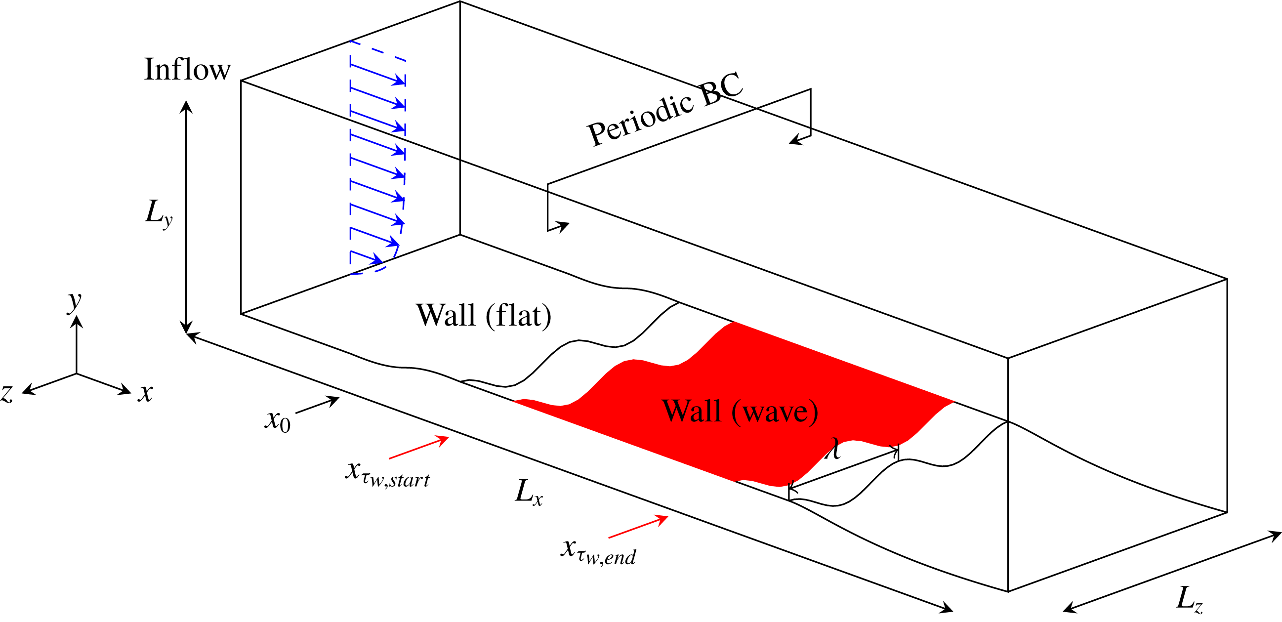
An overview of the set-up is given in figure 6. The dimensions of the physical domain are
 $L_{x}=190\unicode[STIX]{x1D703}$
,
 $L_{y}=105\unicode[STIX]{x1D703}$
and
 $L_{z}=21.65\unicode[STIX]{x1D703}$
. At the inflow of the domain, the reformulated synthetic turbulence generation (RSTG) method by Roidl, Meinke & Schröder (Reference Roidl, Meinke and Schröder2013) is used to prescribe a fully turbulent inflow distribution with an adaptation length of less than five boundary layer thicknesses
 $\unicode[STIX]{x1D6FF}_{99}$
, such that a natural turbulence state is achieved at
 $x_{0}$
, which marks the onset of the actuation. Characteristic outflow conditions are applied at the downstream and upper boundary of the domain and periodic conditions are used in the spanwise direction. On the wall, no-slip conditions are imposed and the wall motion is described by
 $$\begin{eqnarray}y^{+}|_{wall}(x,z^{+},t^{+})=g(x)A^{+}\cos \left(\frac{2\unicode[STIX]{x03C0}}{\unicode[STIX]{x1D706}^{+}}z^{+}+\frac{2\unicode[STIX]{x03C0}}{T^{+}}t^{+}\right),\end{eqnarray}$$
where
 $A^{+}=Au_{\unicode[STIX]{x1D70F}}/\unicode[STIX]{x1D708}$
is the amplitude,
 $\unicode[STIX]{x1D706}^{+}=\unicode[STIX]{x1D706}u_{\unicode[STIX]{x1D70F}}/\unicode[STIX]{x1D708}$
the wavelength and
 $T^{+}=Tu_{\unicode[STIX]{x1D70F}}^{2}/\unicode[STIX]{x1D708}$
the period of the travelling wave in inner coordinates, i.e. scaled by the kinematic viscosity
 $\unicode[STIX]{x1D708}$
and the friction velocity
 $u_{\unicode[STIX]{x1D70F}}(x_{0})$
of the non-actuated reference case. The piecewise defined function
 $$\begin{eqnarray}g(x)=\left\{\begin{array}{@{}ll@{}}0,\quad & \text{if }x<-5,\\ {\displaystyle \frac{1}{2}}\left[1-\cos \left({\displaystyle \frac{\unicode[STIX]{x03C0}(x+5)}{10}}\right)\right],\quad & \text{if }-5\leqslant x<5,\\ 1,\quad & \text{if }5\leqslant x<130,\\ {\displaystyle \frac{1}{2}}\left[1+\cos \left({\displaystyle \frac{\unicode[STIX]{x03C0}(x-130)}{10}}\right)\right],\quad & \text{if }130\leqslant x<140,\\ 0,\quad & \text{otherwise}\end{array}\right.\end{eqnarray}$$
enables a smooth streamwise transition from a flat non-actuated to an actuated wall and vice versa. Apart from the reference case without any wall actuation, i.e.
 $A^{+}=0$
and
 $T^{+}=0$
, 37 parameter combinations of
 $\unicode[STIX]{x1D706}^{+}$
,
 $T^{+}$
and
 $A^{+}$
are considered (see table 3). Most parameter points were generated using Latin hypercube sampling.
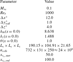
The physical domain is discretized by a structured body-fitted grid with a resolution of
 $\unicode[STIX]{x0394}x^{+}=12$
in the
 $x$
-direction,
 $\unicode[STIX]{x0394}y^{+}|_{wall}=1.0$
in the
 $y$
-direction using gradual coarsening with increasing distance from the wall and
 $\unicode[STIX]{x0394}z^{+}=4.0$
in the
 $z$
-direction. This nearly direct numerical simulation (DNS)-like resolution guarantees the capture of all relevant turbulent scales and allows a smooth representation of the wavy wall. In total, the grid consists of
 $n=732\times 131\times 250\approx 24\times 10^{6}$
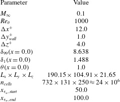
cells. The details of the flow conditions and grid parameters are summarized in table 2.
Overview of the physical domain of the actuated turbulent boundary layer flow, where
 $L_{x}$
,
 $L_{y}$
and
 $L_{z}$
are the dimensions of the domain in the Cartesian directions,
 $\unicode[STIX]{x1D706}$
is the wavelength of the spanwise travelling wave,
 $x_{0}$
marks the onset of the actuation and
 $x_{\unicode[STIX]{x1D70F}_{w},start}$
and
 $x_{\unicode[STIX]{x1D70F}_{w},end}$
denote the interval of the integration of the wall-shear stress
 $\unicode[STIX]{x1D70F}_{w}$
.

Flow and grid parameters of the non-actuated reference case and the 37 actuated cases.
3.2.2 Large-eddy simulation solver
The actuated turbulent boundary layer flow is simulated using a finite volume approximation of the unsteady compressible Navier–Stokes equation on a structured body-fitted mesh. A second-order accurate formulation of the inviscid fluxes using the advection upstream splitting method (AUSM) by Liou & Steffen (Reference Liou and Steffen1993) is applied. The cell-surface values of the flow quantities are reconstructed from the surrounding cell-centre values using a monotone upstream scheme for conservation laws (MUSCL) type strategy. The viscous fluxes are discretized by a modified cell-vertex scheme at second-order accuracy. The time integration is performed by a second-order accurate five-stage Runge–Kutta scheme, rendering the overall discretization second-order accurate. The subgrid scales in the large eddy simulation (LES) are implicitly modelled following the monotonically integrated large-eddy simulation approach (Boris et al. Reference Boris, Grinstein, Oran and Kolbe1992), i.e. the numerical dissipation of the AUSM scheme models for the viscous dissipation of the high wavenumber turbulence spectrum (Meinke et al. Reference Meinke, Schröder, Krause and Rister2002b ). Thus, the small-scale structures are not explicitly resolved and the grid is used as a spatial filter resolving the large energy-containing structures in the inertial subrange. To capture the temporal variation of the geometry, the Navier–Stokes equations are written in the arbitrary Lagrangian–Eulerian (ALE) formulation (Hirt, Amsden & Cook Reference Hirt, Amsden and Cook1997) such that the actuated wall can be represented by an appropriate mesh deformation. Additional volume fluxes are determined to satisfy the geometry conservation law (GCL).
The numerical method has been thoroughly validated by computing a wide variety of internal and external flow problems (Rütten, Schröder & Meinke Reference Rütten, Schröder and Meinke2005; Alkishriwi, Meinke & Schröder Reference Alkishriwi, Meinke and Schröder2006; Renze, Schröder & Meinke Reference Renze, Schröder and Meinke2008; Statnikov, Meinke & Schröder Reference Statnikov, Meinke and Schröder2017). Analyses of drag reduction in turbulent boundary layer flow have been performed for riblet structured surfaces (Klumpp, Meinke & Schröder Reference Klumpp, Meinke and Schröder2010a ) and for travelling transversal surface waves (Klumpp, Meinke & Schröder Reference Klumpp, Meinke and Schröder2011; Koh et al. Reference Koh, Meysonnat, Statnikov, Meinke and Schröder2015a ,Reference Koh, Meysonnat, Meinke and Schröder b ; Meysonnat et al. Reference Meysonnat, Roggenkamp, Li, Roidl and Schröder2016). The quality of the results confirms the validity of the approach for the current flow problem.
3.2.3 Attractor data
Firstly, the simulation of the reference set-up is run for
 $tU_{\infty }/\unicode[STIX]{x1D703}\approx 650$
convective units until a quasi-steady state of the drag evolution is observed. Then, the average drag of the reference set-up is measured for the next
 $\unicode[STIX]{x0394}tU_{\infty }/\unicode[STIX]{x1D703}\approx 1000$
convective units. Subsequently, the actuated cases are initiated using an intermediate solution from the reference case and a quick transition from the flat wall to the fully deflected wall is enforced. When a new quasi-steady state of the friction drag is obtained, i.e. after
 $\unicode[STIX]{x0394}tU_{\infty }/\unicode[STIX]{x1D703}\approx 150$
convective units, the drag of each actuated case is averaged over a period of
 $\unicode[STIX]{x0394}tU_{\infty }/\unicode[STIX]{x1D703}\approx 800$
convective units. The relative drag reduction for the
 $i$
th test case
 $$\begin{eqnarray}\unicode[STIX]{x0394}c_{d,i}=\frac{\displaystyle \int _{A,na}\unicode[STIX]{x1D70F}_{w,na}\,\text{d}A-\displaystyle \int _{A,i}\unicode[STIX]{x1D70F}_{w,i}\,\text{d}A}{\displaystyle \int _{A,na}\unicode[STIX]{x1D70F}_{w,na}\,\text{d}A}\cdot 100,\end{eqnarray}$$
is computed by integrating the wall-shear stress distribution
 $\unicode[STIX]{x1D70F}_{w}$
over the wetted surface
 $A$
in the interval
 $x\in [x_{\unicode[STIX]{x1D70F}_{w},start},x_{\unicode[STIX]{x1D70F}_{w},end}]$
of the non-actuated reference (subscript
 $na$
) and the actuated set-ups (subscript
 $i$
). The values of the relative drag reduction
 $\unicode[STIX]{x0394}c_{d}$
and the skin-friction reduction
 $\unicode[STIX]{x0394}c_{f}$
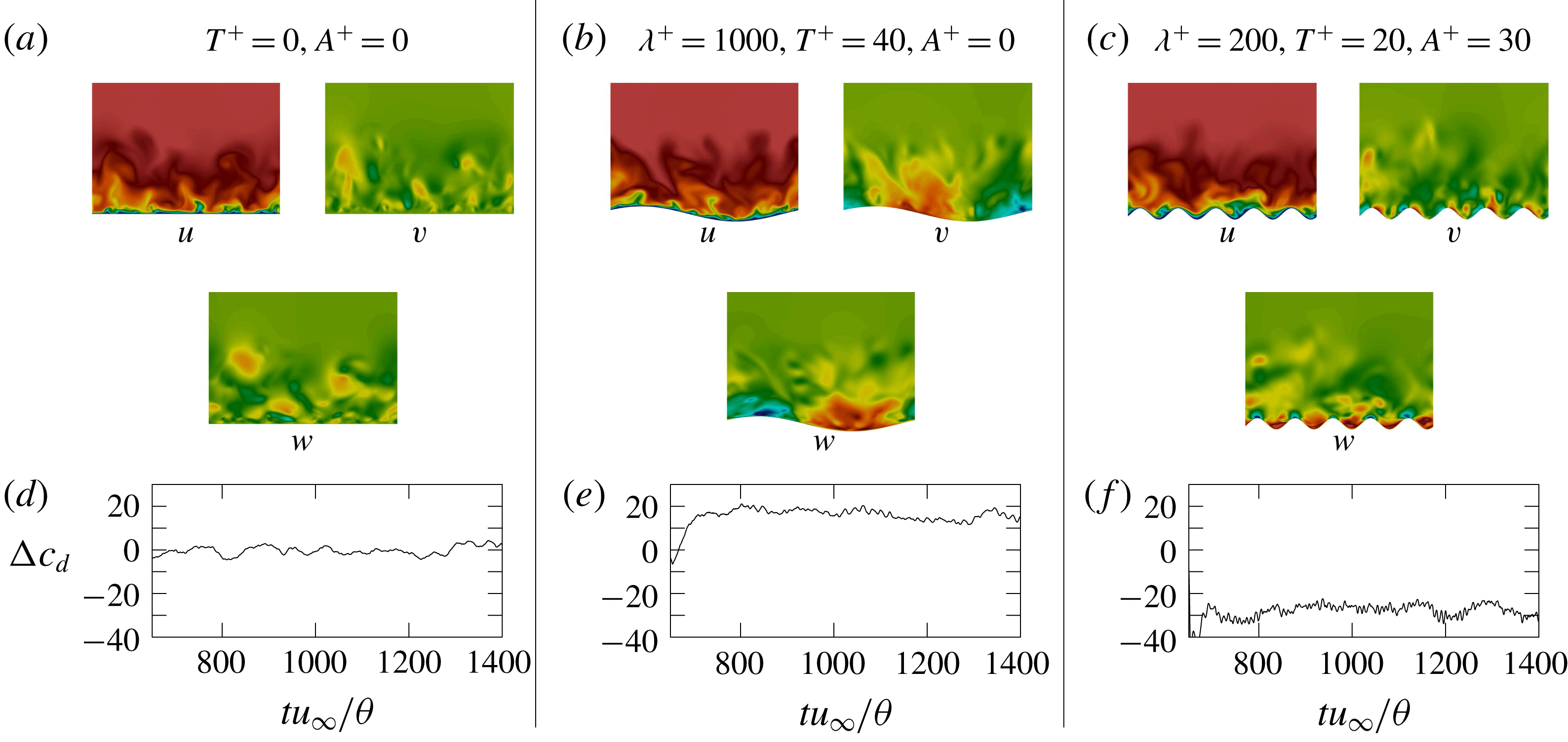
, i.e. the drag reduction without considering the increase in the wetted surface, of the various amplitude, wavenumber and period prescriptions are listed in table 3. An exemplary illustration of the impact of the moving surface on the near-wall velocity field and the friction drag development is given in figure 7 for the reference case
 $N_{1}$
, the case with the highest drag reduction
 $N_{24}$
and the case with the lowest drag reduction
 $N_{2}$
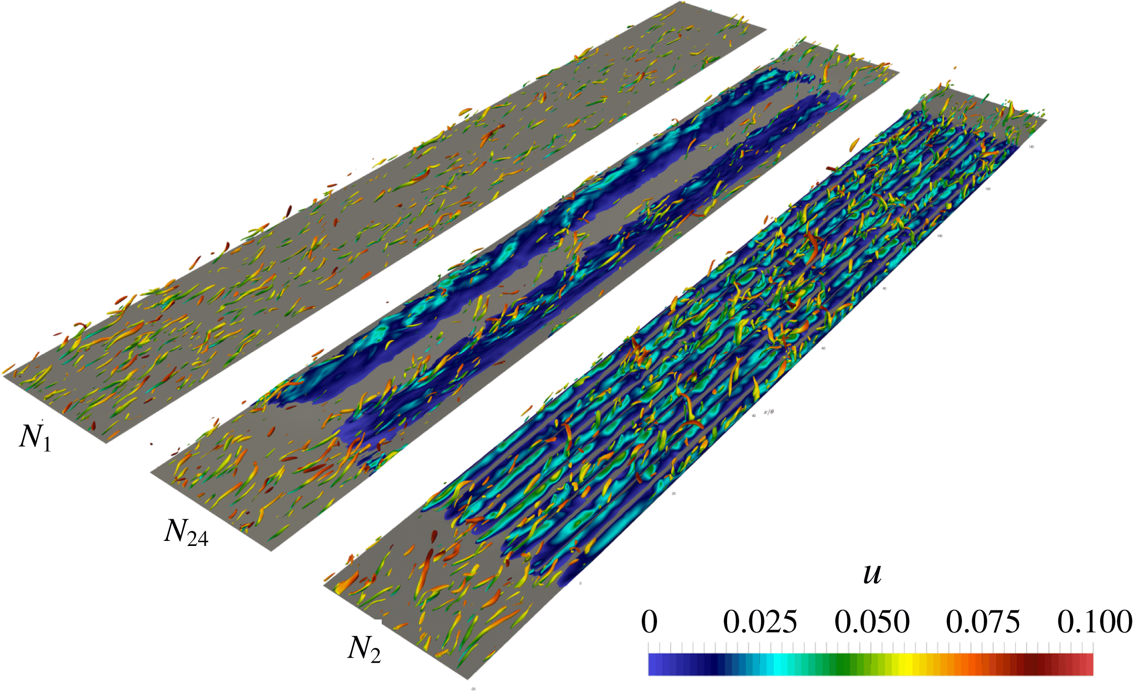
. In figure 8, the variation of the turbulent structures in the near-wall region of these three cases is shown. The comparative juxtaposition of the data evidences the decrease of the turbulent structures for the
 $N_{24}$
case.
Illustration of the turbulent boundary layer flow: (a,d) non-actuated reference case
 $N_{1}$
, (b,e) actuated case with highest drag reduction
 $N_{24}$
and (c,f) actuated case with lowest drag reduction
 $N_{2}$
; (a–c) contour plots of the instantaneous Cartesian velocity components
 $u$
,
 $v$
and
 $w$
in a
 $y{-}z$
plane at
 $x/\unicode[STIX]{x1D703}\approx 65$
; (d–f) time evolution of the instantaneous relative drag reduction
 $\unicode[STIX]{x0394}c_{d}$
.

Contour plot of the
 $\unicode[STIX]{x1D706}_{2}$
-criterion (Jeong & Hussain Reference Jeong and Hussain1995), coloured by the instantaneous streamwise velocity, for three turbulent boundary layer flows; non-actuated reference case
 $N_{1}$
, actuated highest drag reduction case
 $N_{24}$
, actuated lowest drag reduction case
 $N_{2}$
.

The snapshots for the computation of the POD modes are obtained in a subdomain spanning from
 $x=15\unicode[STIX]{x1D703}$
to
 $x=120\unicode[STIX]{x1D703}$
, from the wall to a thickness of
 $y=15.4\unicode[STIX]{x1D703}$
and over the full spanwise extent of the computational domain. That is, the subdomain covers the complete boundary layer over the actuated part of the wall, excluding the zones of spatial transition. The data are collected at the post-transient states with a sampling period of
 $\unicode[STIX]{x0394}tU_{\infty }/\unicode[STIX]{x1D703}\approx 0.94$
.
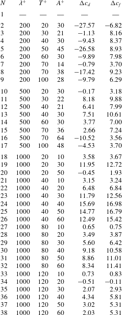
Actuation parameters of the turbulent boundary layer simulations, where each set-up is denoted by a case number
 $N$
. The quantity
 $\unicode[STIX]{x1D706}^{+}$
is the spanwise wavelength of the travelling wave,
 $T^{+}$
is the period and
 $A^{+}$
is the amplitude, all given in inner units, i.e. non-dimensionalized with the kinematic viscosity
 $\unicode[STIX]{x1D708}$
and the friction velocity
 $u_{\unicode[STIX]{x1D70F}}$
. Each block includes set-ups with varying period and amplitude for a constant wavelength. The list includes the values of the averaged relative drag reduction
 $\unicode[STIX]{x0394}c_{d}$
, and the averaged relative skin-friction reduction
 $\unicode[STIX]{x0394}c_{f}$
.

4 Comparison of fluidic pinball attractors with different control laws
The comparison of fluidic pinball attractors is performed following the proposed methodology of the previous section. For simplicity and consistency, we follow the coarse-grained data comparison displayed in the centre and bottom row of figure 1. Firstly, in § 4.1, the cluster analysis is performed. Sections 4.2 and 4.3 present the metric of attractor overlap and associated proximity maps. It should be noted that the analysis is only based on converged post-transient data while the shown temporal dynamics includes also the actuation transients.
4.1 Cluster analysis
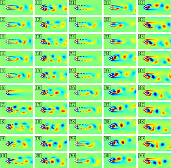
Cluster centroids of the fluidic pinball simulation. The centroids are sorted in order of appearance neglecting the first 50 time units (transients) of each phase. The visualization depicts the vorticity distribution: green, red and blue represent vanishing, positive and negative values, respectively.

Cluster affiliation
 $k$
of the fluidic pinball simulation as a function of time
 $t$
. The applicable control laws are described in table 1 and the corresponding centroid
 $\boldsymbol{c}_{k}$
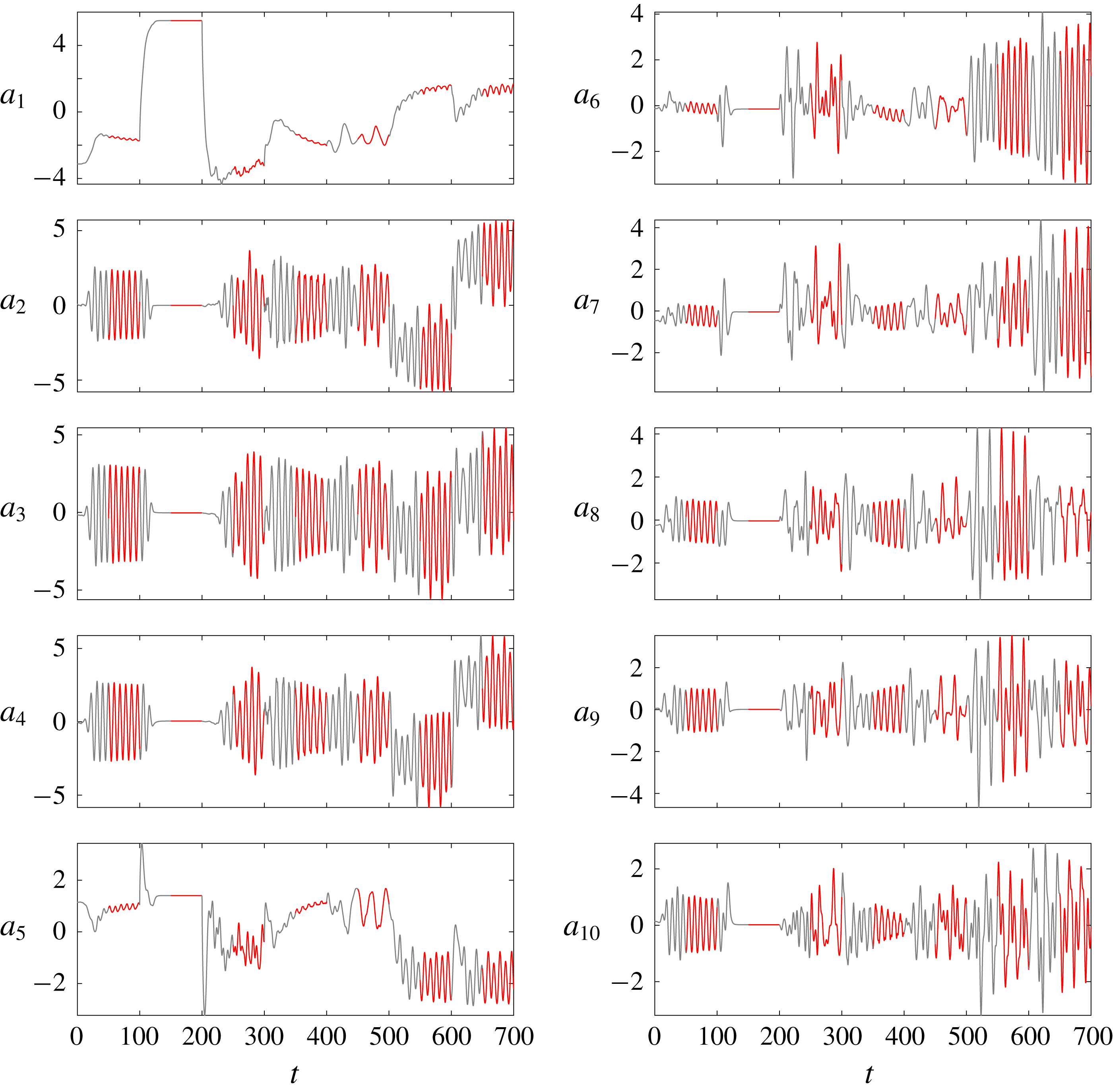
is depicted in figure 9. By construction, new cluster indices are a monotonically increasing function of time, neglecting the initial actuation transients. Grey curve sections correspond to transients while red sections mark the post-transient data taken for the analysis.

Figure 9 illustrates 50 centroids distilled from
 $7\times 500$
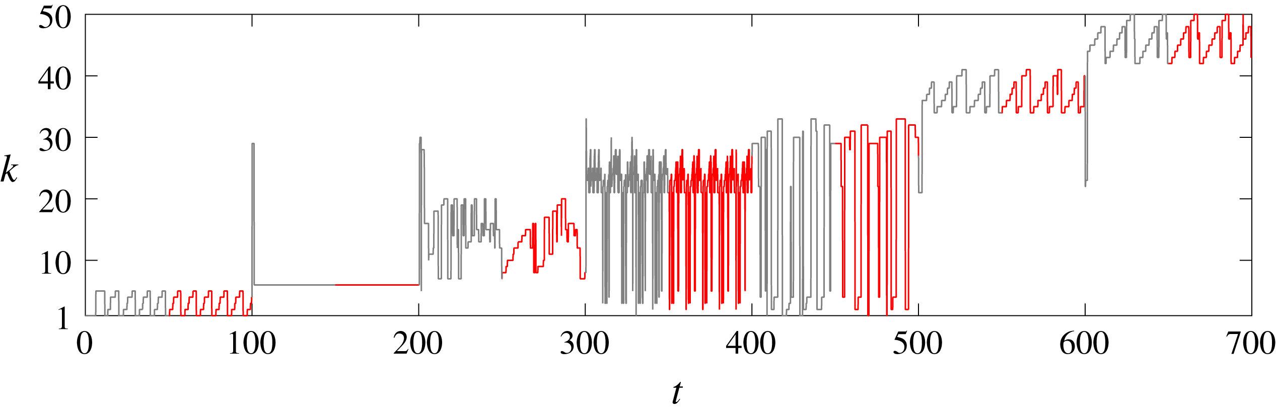
post-transient snapshots. The cluster affiliation as a function of time is shown in figure 10. This affiliation illustrates the role of each centroid (figure 9) in the post-transient behaviours of control laws I–VII of table 1. Clusters 1–5 describe unforced vortex shedding of phase I (see figure 9). We emphasize that the centroids are only meant to resolve converged attractor data and that the presentation of the transient dynamics shall only indicate the transient times. The stabilized boat tailing of phase II is described by a single centroid
 $k=6$
. Base bleed (phase III) is resolved by the new centroids 7–20, indicating that base bleed leads to significantly different vortex shedding structures. High-frequency (phase IV) and low-frequency forcing (phase V) can be resolved with the centroids of unforced vortex shedding and of base-bleed actuation. Low-frequency forcing leads to a wider wake, like base bleed, and has more overlap with the base-bleed dynamics. The new centroids 34–41 resolve the positive Magnus effect (phase VI) while centroids 42–50 the negative Magnus effect (phase VII). As physical intuition suggests, the strong deflected wake has no overlap with forced states which are symmetric or statistically symmetric.
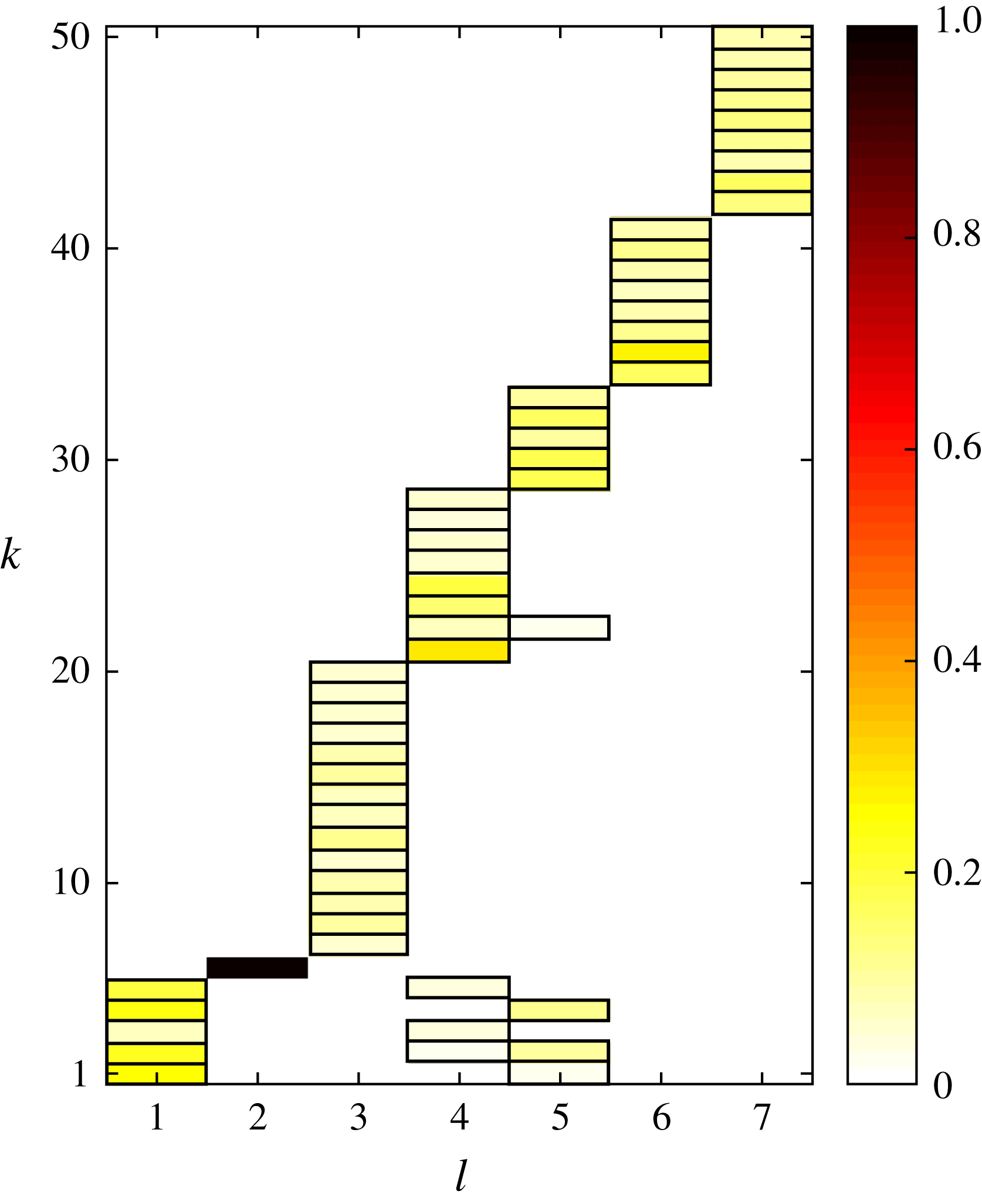
Figure 11 displays the population of each cluster by the seven different dynamics. Probabilities below 1 % are kept white. The probability distributions for each attractor are far from being uniform. This behaviour is different from single attractor cluster analyses, where all clusters are generally populated (Kaiser et al.
Reference Kaiser, Noack, Cordier, Spohn, Segond, Abel, Daviller, Östh, Krajnović and Niven2014). In contrast, considering the whole simulation results in the total probability
 $P_{k}=P_{k}^{1}+\cdots +P_{k}^{7}$
which is non-zero for any cluster
 $k$
. Note that one cluster may be populated by different attractor dynamics.
Population probabilities of the clusters for the seven fluidic pinball phases (table 1). The abscissa denotes the phase
 $l$
and the ordinate the cluster index
 $k$
. Each box represents a non-vanishing probability. The yellow to red tones indicate the population probability
 $P_{k}^{l}$
from (2.17). Probabilities below 1 % are kept white. Note that steady boat tailing (
 $l=2$
) is represented by a single centroid.

4.2 Metric of attractor overlap
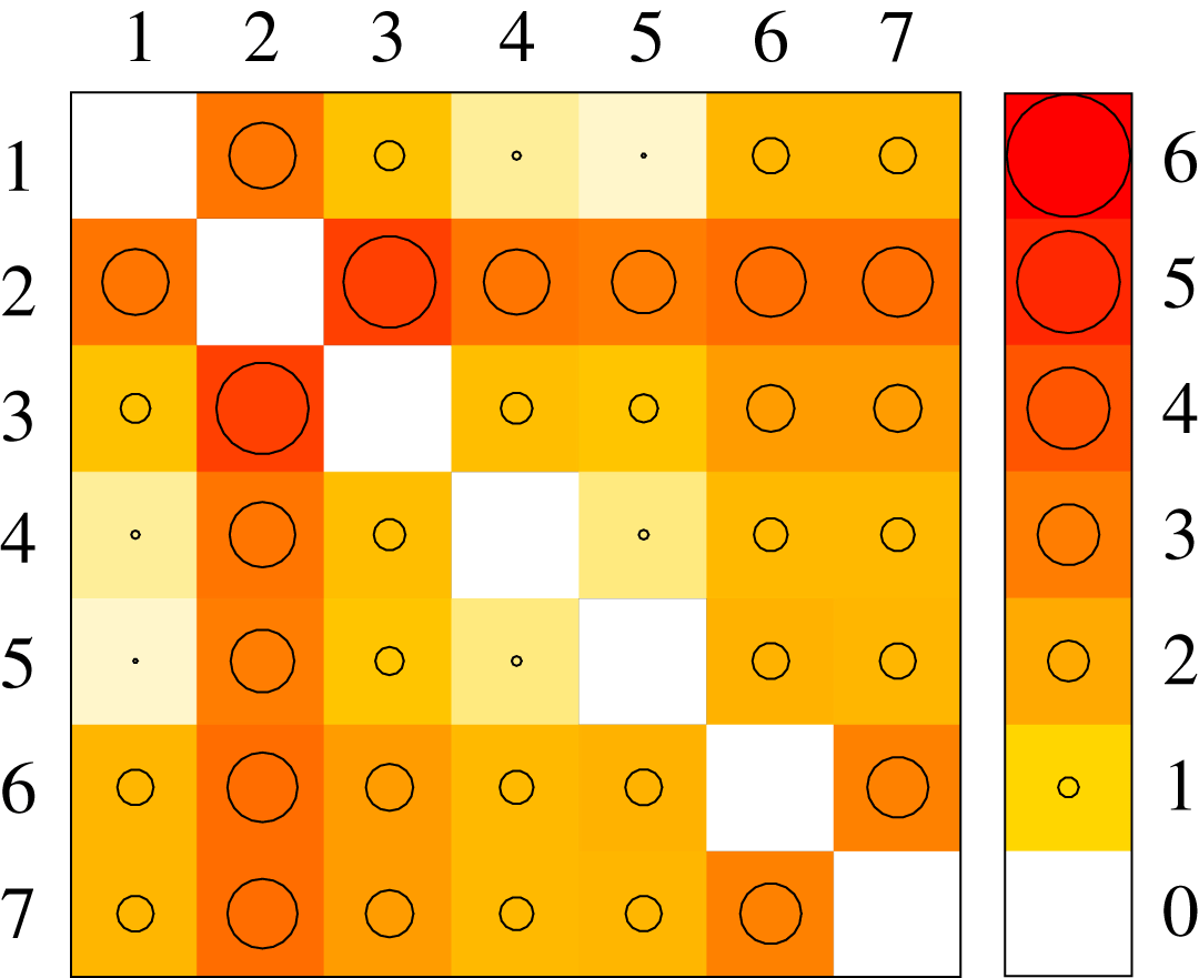
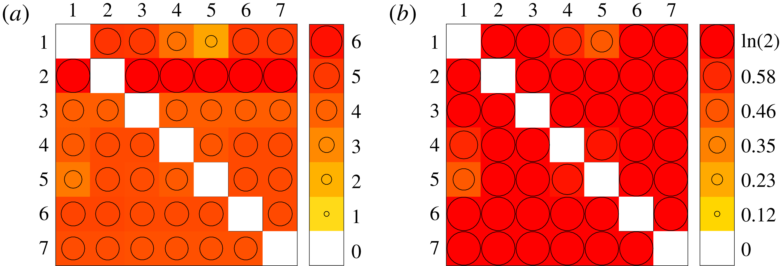
The metric of attractor overlap for the seven operating conditions is displayed in figure 12. The positive (semi)definiteness implies the vanishing elements in the diagonal and non-negative values elsewhere. The symmetry condition leads to the corresponding symmetry of the matrix. The values of the metric are based on the Hilbert-space norm (2.5) and an averaging process over the two attractors (2.1). Hence, the fluctuation level, i.e. twice the fluctuation energy, 2TKE, represents a natural reference value for the square of the metric. Values which are at least one order of magnitude smaller correspond to similar attractors. For the unforced fluidic pinball configuration, the fluctuation level is
 $2\text{TKE}=17.80$
. Hence, a MAO value of
 $\sqrt{2\text{TKE}}=4.22$
can be considered as reference scale for closeness.
Natural vortex shedding (
 $l=1$
) is seen to be close to high- and low-frequency forcing (
 $l=4,5$
), as the metric is a tiny value of the maximum (small circles). This closeness is corroborated by the probability distributions figure 11: the three states share joint clusters. In contrast, the wake stabilized with boat tailing shares no centroids with the other six operating conditions and has a large MAO distance to them. The values are comparable or exceed the reference scale. Similarly, the positive and negative Magnus effect (
 $l=6,7$
) have a large distance to each other, as expected from the opposite deflections of the wake in figure 5 and the empty overlap of both attractors, i.e. no shared clusters in figure 11.
Metric of attractor overlap (2.18) for the seven control laws of the fluidic pinball (table 1). The value of
 $D_{geom}(\boldsymbol{P}^{l},\boldsymbol{P}^{n})$
is shown in the
 $l$
th row and
 $n$
th column as colour code from white to red and by the size of the circle as illustrated by the caption on the right.

4.3 Proximity maps
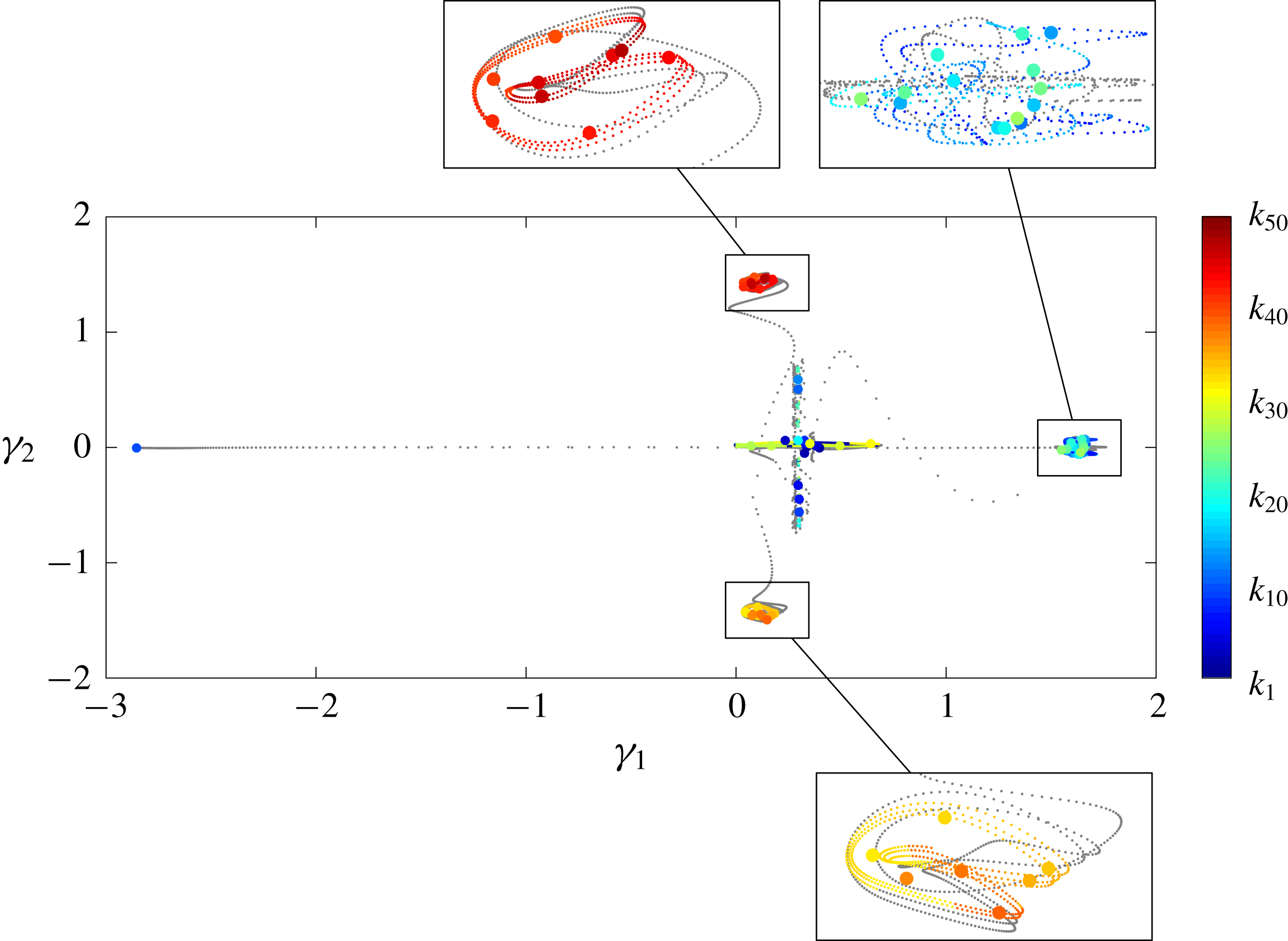
Proximity map of the fluidic pinball showing the centroids (large circles) together with snapshots (small circles). Snapshots from transients are displayed as grey dots, while the data for the analysis are colour coded by cluster affiliation.

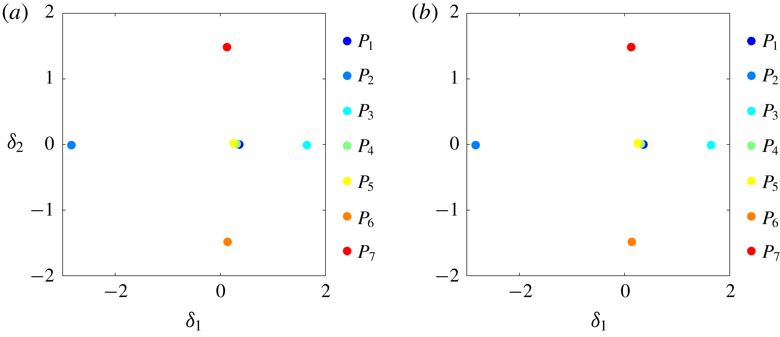
Figure 13 displays all centroids and all snapshots in a proximity map following § 2.3. Phase I–V attractors are located on the
 $\unicode[STIX]{x1D6FE}_{2}=0$
line. These flows are statistically symmetric with respect to the
 $x$
-axis and have, correspondingly, vanishing average lift. Phases VI and VII correspond to positive and negative Magnus effects associated with negative and positive average lift, respectively. These phases are mirror-symmetrically located in the lower and upper region. The second feature coordinate
 $\unicode[STIX]{x1D6FE}_{2}$
is clearly related to averaged lift. The lift values of all phases are displayed in figure 5.
The boat-tailed (phase II) and base-bleed dynamics (phase III) represent the minimal and maximum drag states of considered dynamics, referring again to figure 5. These attractors are on the leftmost and rightmost sides near the
 $\unicode[STIX]{x1D6FE}_{1}$
-axis, respectively. The other attractors have similar drag and have
 $\unicode[STIX]{x1D6FE}_{1}\approx 0$
. Summarizing, the first feature coordinate is strongly correlated to drag. It should be noted that the automatically determined feature coordinates are strongly linked to aerodynamic forces although the forces did not enter the multi-dimensional scaling analysis.
Attractor proximity map of the fluidic pinball: (a) based on the snapshot-based MAO (2.5) and (b) on a cluster-based MAO (2.18) with
 $K=50$
clusters. The points
 $P_{1}\ldots P_{7}$
correspond to the seven control laws in table 1. Note that the snapshot-based MAO represents a cluster-based MAO with maximum number of clusters.

The proximity map for the attractors based on MAO is depicted in figure 14. Figure 14(a) corresponds to the snapshot-based definition, i.e. the most accurate metric while figure 14(b) corresponds to the coarse cluster-based estimate. By construction of the proximity map, the distances between the feature vectors of the seven attractors are similar to the MAO metric values displayed in the matrix of figure 12. Both proximity maps are virtually indistinguishable, thus showing the accuracy of the cluster-based approximation. Varying the cluster resolution in a wide range
 $K\in \{25,50,100\}$
corroborates the robustness of the cluster-based MAO: for all values, the proximity maps are an excellent approximation of the snapshot-based version.
The feature coordinate
 $\unicode[STIX]{x1D6FF}_{1}$
correlates with the drag and
 $\unicode[STIX]{x1D6FF}_{2}$
with the average lift – as in figure 13. These feature coordinates are quantitatively similar to the snapshot and centroid proximity maps (figure 13). This quantitative similarity indicates the robustness of the multi-dimensional scaling for the construction of proximity maps. Another corroboration of the robustness is the symmetry properties of the proximity maps: statistically symmetric flow changes of the attractor mean are characterized by
 $\unicode[STIX]{x1D6FE}_{1}$
and
 $\unicode[STIX]{x1D6FF}_{1}$
while the statistically anti-symmetric changes are parameterized by
 $\unicode[STIX]{x1D6FE}_{2}$
and
 $\unicode[STIX]{x1D6FF}_{2}$
. No symmetry constraints have been imposed on the data processing.
5 Comparison of turbulent boundary layers at different wall actuations
We analyse the three-dimensional flow data generated by 38 simulations of the actuated turbulent boundary layer using the cluster-based MAO methodology. In § 5.1 we present the cluster analysis of the 38 attractors. In §§ 5.2 and 5.3 the MAO analysis and proximity maps for snapshots, centroids and attractors are illustrated.
5.1 Cluster analysis
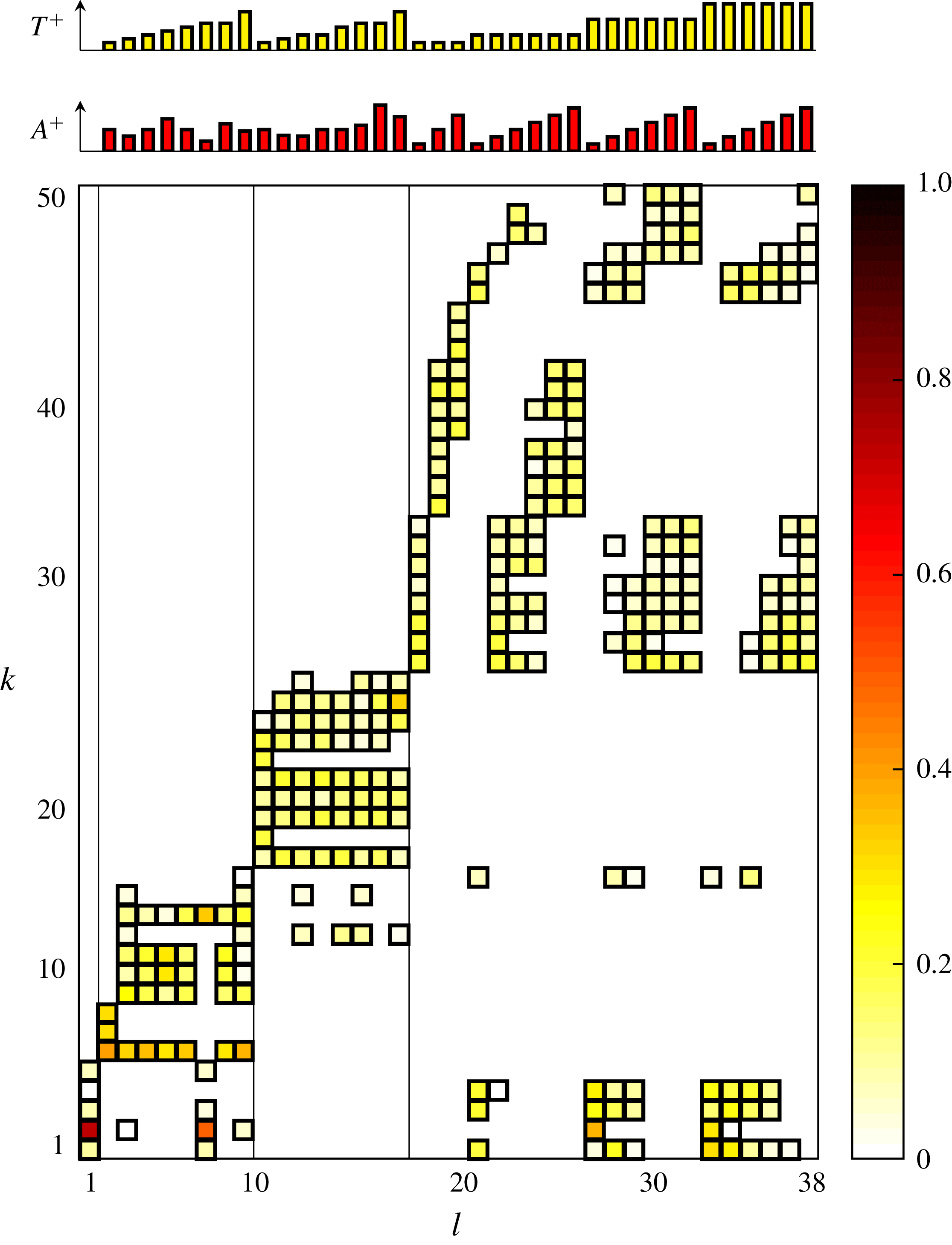
Population probabilities of the clusters for the 38 turbulent boundary layer simulations (see table 3). The abscissa denotes the data set
 $l$
and the ordinate the cluster index
 $k$
. Each box represents a non-vanishing probability. The yellow to red tones indicate the population probability or relative frequency
 $P_{k}^{l}$
from (2.17). Probabilities below 1 % are kept white. The actuation wavelength is indicated by the three vertical line separating simulations with no actuation,
 $\unicode[STIX]{x1D706}^{+}=200$
,
 $\unicode[STIX]{x1D706}^{+}=500$
and
 $\unicode[STIX]{x1D706}^{+}=1000$
from left to right. The actuation amplitude
 $A^{+}$
and time
 $T^{+}$
are shown in the top caption.

Figure 15 displays the probability distribution of each attractor to pass through a given cluster. Again, probabilities below 1 % are kept white. All attractors have pairwise different cluster compositions. The unforced reference
 $l=1$
occupies the first five clusters. The attractors
 $l=2,\ldots ,9$
corresponding to a spanwise wavelength
 $\unicode[STIX]{x1D706}=200$
populate clusters
 $k=5,\ldots ,16$
. The attractor
 $l=7$
with low actuation amplitude shares four of five clusters with the unforced flow and populates one new cluster
 $k=14$
. The simulations with a spanwise wavelength
 $\unicode[STIX]{x1D706}^{+}=500$
(
 $l=10,\ldots ,17$
) pass through the new clusters
 $k=18,\ldots ,26$
. These attractors have no overlap with the unforced reference and share few states with the previous group at low-wavelength actuation. The long-wavelength actuation (
 $\unicode[STIX]{x1D706}^{+}=1000$
) populates the new clusters
 $l=27,\ldots ,50$
. This group shares only one cluster
 $(l=16)$
with the medium-wavelength group but may have significant overlap with the unforced reference. This is particularly true for low-amplitude (
 $A^{+}=10$
) actuations at
 $l=21$
, 27 and 33. It should be noted that the MAO methodology displays the overlap between attractors in a computer- and human-interpretable form.
5.2 Metric of attractor overlap

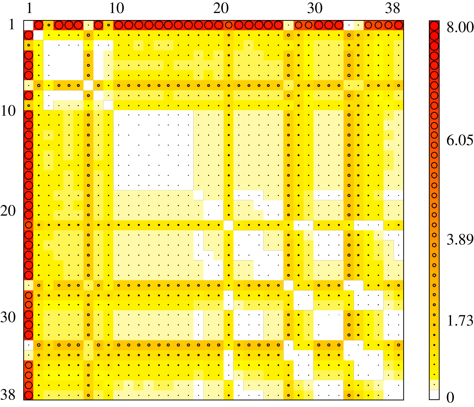
Figure 16 displays the geometric distance between the attractors based on MAO. Evidently the diagonal vanishes by definition. In complete analogy to the fluidic pinball, the reference for a large scale can be taken to be the fluctuation amplitude
 $\sqrt{2\text{TKE}}=0.8767$
of the unforced flow
 $(A=0)$
, noting that actuation may increase this amplitude by one order of magnitude. Most of metric values are in this range or lower.
The unforced reference
 $l=1$
is seen to be very different from most other attractors. Attractors 2 to 6 are very close to each other, which can be expected because of their same actuation wavelength
 $\unicode[STIX]{x1D706}^{+}=200$
. Again, attractors 10 to 17 corresponding to wavelength
 $\unicode[STIX]{x1D706}^{+}=500$
display significant similarity, i.e. a low MAO. The group of actuated cases with large wavelength
 $\unicode[STIX]{x1D706}^{+}=1000$
show less similarity, which is consistent with the discussed overlap from the previous figure. Attractors 7, 21, 27 and 33 have low actuation amplitude and share similar characteristics with the unforced reference, as may be expected.
5.3 Proximity map
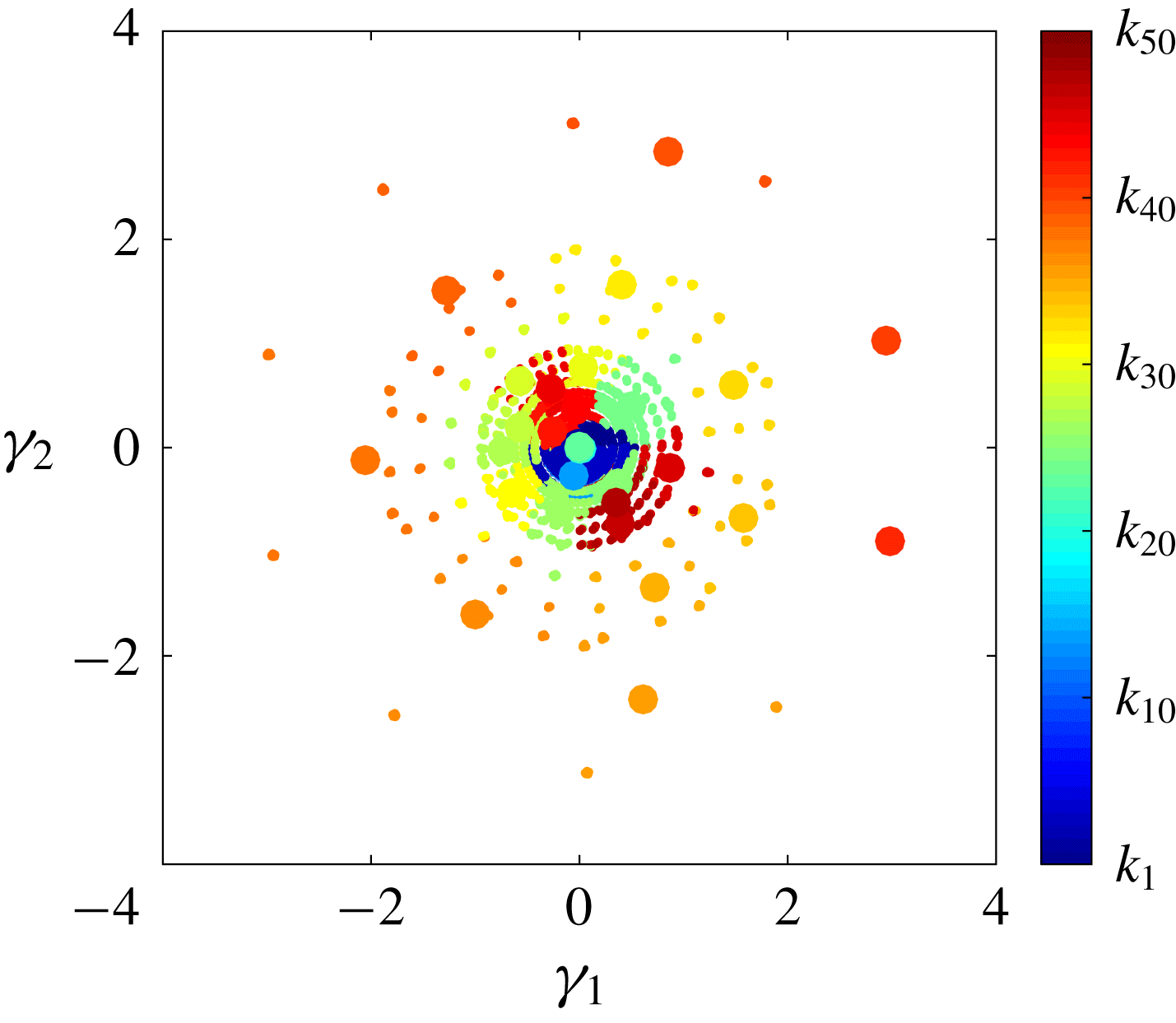
Proximity map of the actuated turbulent boundary layer. The figure displays the centroids (large circles) together with snapshots (small circles). The data for the analysis are colour coded by cluster affiliation.

Figure 17 visualizes the distance between the centroids and snapshots. Actuations at low wavelengths (small
 $k$
) are close to the origin while large-wavelength actuation (large
 $k$
) may populate circular regions in the periphery. A closer analysis reveals that
 $\unicode[STIX]{x1D6FE}_{1}$
,
 $\unicode[STIX]{x1D6FE}_{2}$
correspond to the first POD mode amplitudes
 $a_{1}$
,
 $a_{2}$
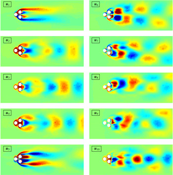
computed from all snapshot data together. These POD mode amplitudes are nearly periodic, particularly for large actuation amplitudes.
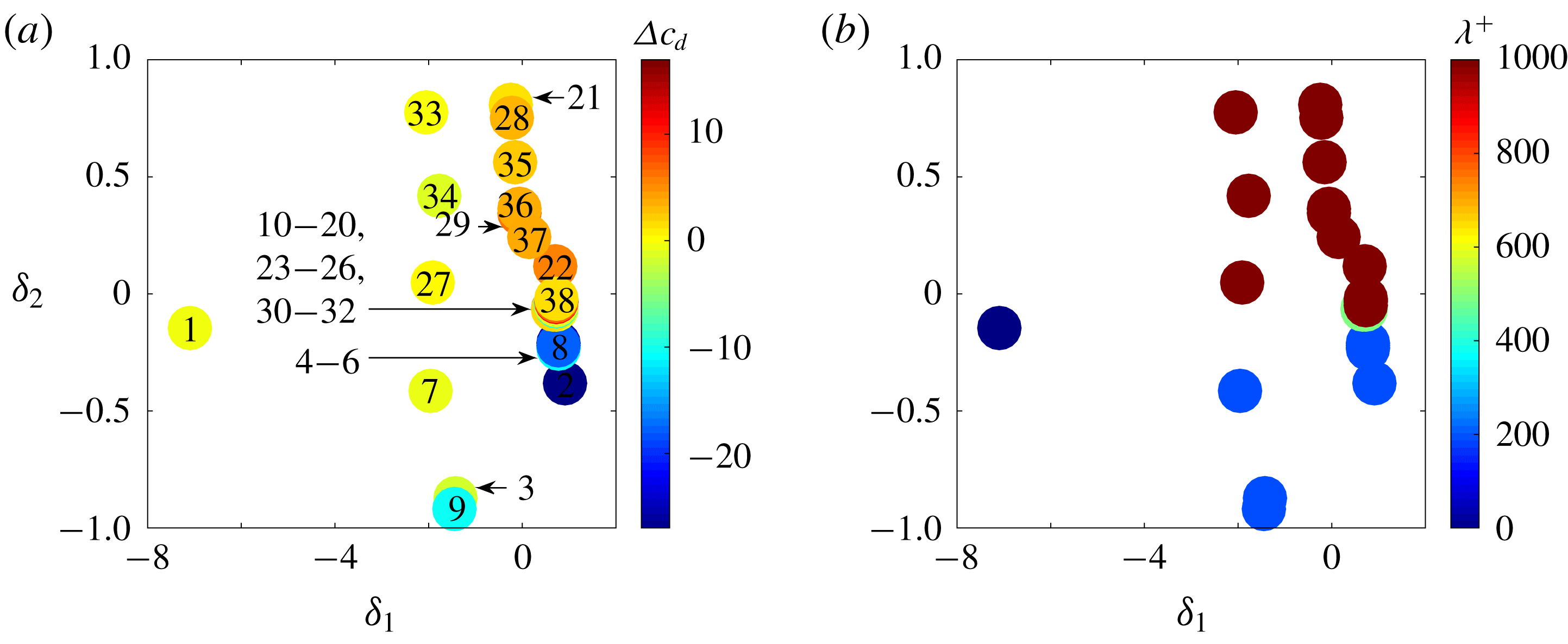
Attractor proximity map of the turbulent boundary layer simulations (see table 3): (a) colour coded with relative drag reduction
 $\unicode[STIX]{x0394}c_{D}$
; (b) colour coded with wavelength
 $\unicode[STIX]{x1D706}^{+}$
. The actuation parameters of each symbol is indicated in (a) by a number corresponding to the index from table 3.

Figure 18 displays the proximity map of the attractors based on MAO as shown in figure 16. From figure 18(a) the first feature coordinate
 $\unicode[STIX]{x1D6FF}_{1}$
is linked to the drag reduction for the attractors: for
 $\unicode[STIX]{x1D6FF}_{1}<0$
actuation has little effect on drag but for
 $\unicode[STIX]{x1D6FF}_{1}\geqslant 0$
these changes are significant – positive for
 $\unicode[STIX]{x1D6FF}_{2}>0$
and negative for
 $\unicode[STIX]{x1D6FF}_{2}<0$
. From figure 18(b),
 $\unicode[STIX]{x1D6FF}_{2}$
correlates with the wavelength of the travelling wave. The large wavelengths are located in the top half of the plot. As seen in the fluidic pinball, the MAO-based attractor proximity map extracts the aerodynamics and actuation properties without directly including information about them.
6 Conclusions and outlook
We have proposed a novel quantitative measure, termed the metric of attractor overlap (MAO), for the similarity of attractor data. This measure generalizes the Hilbert-space metric for two velocity fields to a metric between two sets with snapshot data. A refined comparison analysis includes proximity maps and coarse graining with clustering.
Our proposed comparison methodology has five discriminating features. Firstly, the difference between two attractors is quantified in a single, non-negative number encapsulating all resolved coherent structures. Secondly, the cluster probability distribution of each attractor identifies shared and disjoint flow states via a manageable number of centroids. Thirdly, the metric of attractor overlap enables the automatic creation of a proximity map from a myriad of attractors. Neighbouring feature points represent attractors with similar flow states, largely separated points indicate attractors with different physics. Fourthly, the approach is compatible with statistical post-processing: the centroids and their probabilities define the mean flow and – in principle – any higher-order moments, like Reynolds stress or fluctuation energy. Even POD modes can be derived from the centroids. Finally, the comparison methodology can be automatized and has little subjective bias. One does not need to decide in advance on a cost function, such as drag power, a frequency filter, such as a low-pass filter, important flow features, such as vortices, just to name a few.
The metric of attractor overlap is only based on two decisions. Firstly, one needs to choose the flow state space, e.g. the velocity field in a domain
 $\unicode[STIX]{x1D6FA}$
. Such a decision is unavoidable for any metric. Secondly, a metric for two flow states is needed. A
 $L^{2}(\unicode[STIX]{x1D6FA})$
Hilbert-space norm appears as a natural candidate. For the optional coarse graining, the number of clusters or, synonymously, the typical size of a cluster needs to be chosen. The coarse-grained metric is found to quickly converge to the snapshot-based one with increasing number of clusters.
The comparison methodology has been applied to the fluidic pinball, the flow around a cluster of three rotating cylinders. The considered attractors include the unforced reference, aerodynamic boat tailing, base bleed, symmetric high-frequency forcing, symmetric low-frequency forcing and a Magnus effect deflecting the wake to both sides. The metric of attractor overlap confirms physical inspection of the seven configurations. Firstly, boat tailing with complete wake suppression differs strongly from all other states. Secondly, both Magnus effects also strongly differ from all other states. Third, unforced vortex shedding and wakes manipulated by base bleed as well as high-frequency and low-frequency forcing have a significant overlap of shared clusters, i.e. are similar.
Particularly noteworthy are the proximity maps of the snapshots and the cluster-based attractors. The trajectory through all seven configurations displays the dynamics very clearly (see figure 5). Surprisingly, the first and second feature coordinates resemble the drag and lift respectively (see figure 14). The features of the snapshots show the reduced drag by boat tailing (
 $P_{2}$
) and the increased drag by base bleed (
 $P_{3}$
) and significant average lift by both Magnus forcing (
 $P_{7}$
and
 $P_{6}$
). The proximity map of the attractor visually elucidates the discussed neighbourhood relations in the first three feature coordinates.
The second application of MAO is an open-loop drag reduction study of a turbulent boundary layer. The operating conditions include the unforced reference and 37 actuations with spanwise travelling waves at different amplitudes and frequencies. The spanwise wavelengths include a small (
 $\unicode[STIX]{x1D706}^{+}=200$
), medium (
 $\unicode[STIX]{x1D706}^{+}=500$
) and large value (
 $\unicode[STIX]{x1D706}^{+}=1000$
). The computational and observation domain are defined by the largest actuation wavelength. The MAO analysis features several highlights. Firstly, the low-amplitude actuations share centroids with the unforced reference in agreement with physical intuition. Secondly, actuations with the same spanwise wavelength show significant overlap. Thirdly, the feature map of the snapshots show low-amplitude states near the centre and large-amplitude actuations populate outer circular regions. The feature coordinates are well aligned with the first two POD mode amplitudes. These modes approximate the phase-averaged flow response to the periodic actuation. Finally, the first feature coordinate of the attractor proximity map correlates well with the drag reduction –as for the fluidic pinball – while the second coordinate depends on the spanwise actuation wavelength.
The observed correlation between first feature coordinate and drag for two independent configurations is surprising as the input data do not contain information about drag. In hindsight, this behaviour may be explained by the strong correlation between the time-averaged flow and the drag – both for the wake and for the boundary layer.
Evidently, the presented MAO comparison encourages numerous other applications, like a comparison between computed and experimental velocity fields and a comparison between flow behaviour under different actuations, e.g. periodic forcing or machine learning control studies (Duriez et al. Reference Duriez, Brunton and Noack2016). The analysis may also be applied to sensor data, e.g. a hot-wire rig, instead of velocity fields.
Future research may significantly extend the MAO methodology. The employed Hilbert-space norm is a good initial choice but highly sensitive to small mode deformations (Noack Reference Noack2016). A small change in wavenumber gives rise to unphysically large differences in the norm. Force-related feature vectors and manifold learning may be one remedy (Loiseau, Noack & Brunton Reference Loiseau, Noack and Brunton2018). Rigorous physics-based criteria for the cluster numbers need to be advanced. The comparison may also be targeted towards single- or multi-objective goals by generalizing the snapshot metric. So far, the comparison only addressed ergodic properties of the attractor, and the snapshot data only needed to be statistically representative and not time resolved. The temporal dynamics of different attractors may be compared using time-resolved snapshots and corresponding Markov models (Kaiser et al. Reference Kaiser, Noack, Cordier, Spohn, Segond, Abel, Daviller, Östh, Krajnović and Niven2014).
Summarizing, a rational automated comparison method has been proposed which holds significant promise for future data assessments. The authors are actively pushing this direction.
Acknowledgements
This work is supported by a public grant overseen by the French National Research Agency (ANR) as part of the ‘Investissement dAvenir’ programme, through the ‘iCODE Institute project’ funded by the IDEX Paris-Saclay, ANR-11-IDEX-0003-02, by the ANR grants ‘ACTIV_ROAD’ and ‘FlowCon’, by the Polish National Center for Research and Development under the grant no. PBS3/B9/34/2015 and by the Bernd Noack Cybernetics Foundation. Additional funds are provided by the German Research Foundation (DFG) under grant nos SE 2504/2-1 and SCHR 309/68-1. Computing resources were provided by the High Performance Computing Center Stuttgart (HLRS) and by the Jülich Supercomputing Center (JSC) within a large-scale project of the Gauss Center for Supercomputing (GSC). E.K. gratefully acknowledges support by the ‘Washington Research Foundation Fund for Innovation in Data-Intensive Discovery’ and a Data Science Environments project award from the Gordon and Betty Moore Foundation (Award no. 2013-10-29) and the Alfred P. Sloan Foundation (Award no. 3835) to the University of Washington eScience Institute. We appreciate valuable stimulating discussions with S. Brunton, N. Kutz, T. Sapsis and the French–German–Canadian–American pinball team: G. Y. Cornejo-Maceda, N. Deng, F. Lussgeeyran, R. Martinuzzi, C. Raibaudo, R. Rolland and L. Pastur. Last but not least, we are deeply indebted to the anonymous referees for their insightful suggestions.
Appendix A. Proper orthogonal decomposition versus clustering
The cluster analysis is compared with the proper orthogonal decomposition (POD) from the same data in the same observation domain. Each snapshot is expanded in terms of the mean flow
 $\boldsymbol{u}_{0}(\boldsymbol{x})$
of all post-transient attractor data and
 $N$
POD modes
 $\boldsymbol{u}_{i}(\boldsymbol{x})$
,
 $i=1,\ldots ,N$
and their corresponding amplitudes
 $a_{i}(t),i=1,\ldots ,N$
 $$\begin{eqnarray}\boldsymbol{u}(\boldsymbol{x},t)\approx \boldsymbol{u}_{0}(\boldsymbol{x})+\mathop{\sum }_{i=1}^{N}a_{i}(t)\boldsymbol{u}_{i}(\boldsymbol{x}).\end{eqnarray}$$
Figures 19 and 20 display the first ten POD modes and their amplitudes, respectively. Mode 1 resolves a base-flow deformation, like a shift mode (Noack et al. Reference Noack, Afanasiev, Morzyński, Tadmor and Thiele2003). Mode 5 represents a symmetric near-field modulation. The other modes have more oscillatory structures. We shall not pause to hypothesize about the physical meaning of these modes. Modes with cleaner frequency content yet near the optimal residual could, for instance, be constructed with recursive dynamic mode decomposition (DMD) (Noack et al. Reference Noack, Stankiewicz, Morzyński and Schmid2016). The cluster analysis resulting in the snapshot cluster affiliation (figure 10) and centroids (figure 9) is physically easier to interpret than the POD.
The POD modes
 $\boldsymbol{u}_{i}(\boldsymbol{x})$
,
 $i=1,\ldots ,10$
. Visualization as in figure 9.

POD amplitudes
 $a_{i}(t)$
,
 $i=1,\ldots ,10$
. Snapshot sequences after the decay of the transients are employed for the analysis (coloured in red).

It may be noted that POD also allows for another metric of attractor overlap. Let
 $p(\boldsymbol{a})$
be the probability distribution associated with one attractor and
 $q(\boldsymbol{a})$
the distribution of another one. Then, the continuous version of the Jensen–Shannon distance (B 4) can be applied. An advantage is that the snapshot distance (2.1) is reflected in the construction of the metric. A disadvantage is the need for approximations to construct a continuous probability distribution from a finite number of snapshots.
Appendix B. Jensen–Shannon distance
Probability distributions can easily be compared using information measures. Let
 $\boldsymbol{Q}=[Q_{1},\ldots ,Q_{K}]$
be a reference probability distribution and
 $\boldsymbol{P}=[P_{1},\ldots ,P_{K}]$
a new measured one. Then, the information gained from
 $\boldsymbol{P}$
with respect to the reference
 $\boldsymbol{Q}$
is quantified by the Kullback–Leibler divergence (Kullback & Leibler Reference Kullback and Leibler1951; Kullback Reference Kullback1959), also called relative entropy,
 $$\begin{eqnarray}D_{KL}(\boldsymbol{P}\Vert \boldsymbol{Q})=\mathop{\sum }_{k=1}^{K}P_{k}\ln \left[\frac{P_{k}}{Q_{k}}\right].\end{eqnarray}$$
Identical probability distributions
 $\boldsymbol{P}=\boldsymbol{Q}$
give rise to a vanishing Kullback–Leibler divergence. Different distributions yield a positive value. If
 $P_{k}=0$
, the term
 $P_{k}\ln P_{k}/Q_{k}$
is interpreted as zero because
 $\lim _{x\rightarrow 0}x\ln x=0$
. Strictly speaking, the Kullback–Leibler divergence is not defined in case there exists a
 $k$
for which
 $Q_{k}=0$
and
 $P_{k}>0$
. One could follow a common practice of smoothing using the absolute discounting method by replacing
 $Q_{k}$
by a small value, e.g.
 $\unicode[STIX]{x1D716}=0.001$
.
The Kullback–Leibler divergence is not symmetric, i.e.
 $D_{KL}(\boldsymbol{P}\Vert \boldsymbol{Q})\not \equiv D_{KL}(\boldsymbol{Q}\Vert \boldsymbol{P})$
. Hence, it cannot serve as a metric. The probability distributions
 $\boldsymbol{P}$
and
 $\boldsymbol{Q}$
may be compared with the Jensen–Shannon divergence which is defined as symmetrized and smoothened Kullback–Leibler divergence
 $$\begin{eqnarray}JSD(\boldsymbol{P},\boldsymbol{Q})={\textstyle \frac{1}{2}}[D_{KL}(\boldsymbol{P}\Vert \boldsymbol{M})+D_{KL}(\boldsymbol{Q}\Vert \boldsymbol{M})],\quad \text{where }\boldsymbol{M}={\textstyle \frac{1}{2}}[\boldsymbol{P}+\boldsymbol{Q}].\end{eqnarray}$$
Equivalently,
 $$\begin{eqnarray}JSD(\boldsymbol{P},\boldsymbol{Q})=\frac{1}{2}\mathop{\sum }_{k=1}^{K}\left(P_{k}\ln \left[\frac{2P_{k}}{P_{k}+Q_{k}}\right]+Q_{k}\ln \left[\frac{2Q_{k}}{P_{k}+Q_{k}}\right]\right).\end{eqnarray}$$
The summation term is interpreted as zero if
 $P_{k}=Q_{k}=0$
or if the numerator of the logarithm argument vanishes. Note that we do not need the
 $\unicode[STIX]{x1D716}$
threshold of the Kullback–Leibler entropy anymore.
The square root of the Jensen–Shannon divergence has all properties of a metric (Endres & Schindelin Reference Endres and Schindelin2003) and is referred to as the Jensen–Shannon distance,
 $$\begin{eqnarray}D_{JS}(\boldsymbol{P},\boldsymbol{Q})=\sqrt{JSD(\boldsymbol{P},\boldsymbol{ Q})}.\end{eqnarray}$$
This distance (B 4) defines an entropic metric of attractor overlap between two attractor data represented by the cluster distributions
 $\boldsymbol{P}$
and
 $\boldsymbol{Q}$
.
Distances between attractors: (a) Kullback–Leibler divergence and (b) Jensen–Shannon divergence based on the cluster probability distribution for each of the seven control phases. The row and column of
 $D_{KL}(P\Vert Q)$
correspond to the first (
 $\boldsymbol{P}$
) and second arguments (
 $\boldsymbol{Q}$
). The value of the divergence is colour coded and indicated by the size of the circle (see the corresponding caption).

Figure 21 displays the Kullback–Leibler and Jensen–Shannon divergences between the seven fluidic pinball attractors. The diagonal entries vanish by definition. Unforced vortex shedding is seen to be similar to high- and low-frequency forcing, as was indicated already by the many shared clusters in figure 10. The difference between unforced shedding, base-bleed dynamics and both Magnus effects is larger as they share no joint clusters. The stabilized boat tailing with a single cluster is seen to be very different from all other phases with no cluster overlap. The Kullback–Leibler divergence is, as expected, not symmetric. For instance. the divergence of boat tailing with respect to base bleed is larger than the other way around. It should be noted that the Jensen–Shannon distance is typically
 $\ln (2)$
(or unity if the base 2 logarithm is used) corresponding to no shared clusters.
The Jensen–Shannon distance is a natural metric for probability distributions. Yet, it is blind to the geometric location of the centroids. Let us assume the first attractor data populate only cluster 1,
 $P_{i}=\unicode[STIX]{x1D6FF}_{i,1}$
, and the second data occupy only cluster 2,
 $Q_{i}=\unicode[STIX]{x1D6FF}_{i,2}$
. In this case,
 $JSD(\boldsymbol{P},\boldsymbol{Q})=\ln 2$
, regardless of whether the centroids are very close or very far from each other. This property makes the Jensen–Shannon distance strongly dependent on the number of clusters or, equivalently, on the typical size of the clusters. For the minimum number of clusters,
 $K=1$
, we have obtained the trivial result
 $P_{1}=Q_{1}=1$
and
 $JSD=0$
. For the maximum number of clusters, each snapshot represents one centroid and defines one cluster. In the generic case of different snapshots, the Jensen–Shannon distance is also
 $\ln 2$
independent of the geometric location of the snapshots. Only a few of the seven fluidic pinball phases share joint clusters and the proximity maps based on (B 4) provide limited physical insight. The metric may be far more meaningful in other cases in which most attractors have significant overlap.