

1. Introduction
The ubiquity of flows where a dispersion of particles is carried by a fluid phase has motivated many theoretical, experimental and numerical studies. Such systems, also referred to as particle-laden flows, are widely encountered in natural and industrial settings. Sediment transport, rain and drop formation, fluidised beds and slurry flows are only a few examples among many where particle-laden flows occur. Analytical treatment of these systems is generally limited to asymptotic cases with very low Reynolds numbers and solid volume fractions, whereas the practical interest usually lies in the opposite end of this spectrum. Conversely, the unprecedented availability of massive computational power in the past two decades has substantially promoted the utility of numerical methods for investigation of particle-laden flows.
In a dispersed multiphase system, particles interact with each other locally on the length scale of the particle diameter  $d$, which could lead to the occurrence of close-range phenomena such as drafting–kissing–tumbling (DKT) due to wake attraction in inertial regimes (Fortes, Joseph & Lundgren Reference Fortes, Joseph and Lundgren1987; Dash & Lee Reference Dash and Lee2015). Interactions of this nature are known to contribute to the formation of particle clusters that extend several diameters (Kajishima & Takiguchi Reference Kajishima and Takiguchi2002; Uhlmann & Doychev Reference Uhlmann and Doychev2014; Fornari, Ardekani & Brandt Reference Fornari, Ardekani and Brandt2018). These structures, in turn, potentially interact with each other and thus bring about an integral length scale that could be one or two orders of magnitude larger than
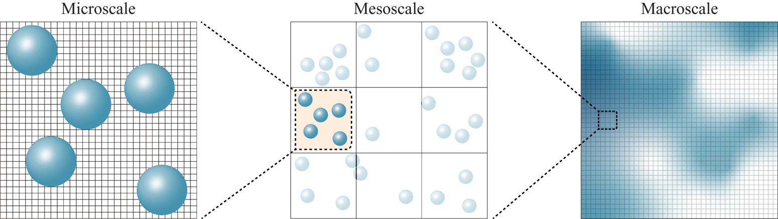
 $d$. Clustering of water droplets in clouds is an interesting natural example, which is known to greatly enhance coalescence and thereby explaining the growth rate of droplets (Collins & Keswani Reference Collins and Keswani2004). On the other hand, clusters have a remarkable effect on particle residence time, and heat and mass transfer in circulating fluidised beds (Louge, Lischer & Chang Reference Louge, Lischer and Chang1990; Wylie & Koch Reference Wylie and Koch2000). A fluidised bed reactor in a fluid catalytic cracking unit is typically 14 m high and 6 m in diameter. Within such a device, fluid–solid interactions and particle collisions in the sub-millimetre scale can directly influence flow structures such as clusters of the order of metres (van der Hoef et al. Reference van der Hoef, van Sint Annaland, Deen and Kuipers2008). The enhancement of local concentration of particles in clusters also leads to increased collision rates. Clearly, the time scale of particle collisions is much shorter than convective or diffusive time scale of the flow, creating yet another level of scale separation. The cascade of such multi-scale interactions modifies the character of particle suspensions and significantly affects quantities of interest, such as settling rate and particle velocity fluctuations (Zaidi, Tsuji & Tanaka Reference Zaidi, Tsuji and Tanaka2014; Zaidi Reference Zaidi2018; Willen & Prosperetti Reference Willen and Prosperetti2019). Due to the presence of a wide range of length scales, a single description of the physics would fail to provide balance between the required complexity or resolution, and the associated computational cost for all involved scales. This is the motivation for development of various numerical methodologies aiming at resolving the flow at three major length scales; namely, the micro-, meso- and macroscale. Such a multi-scale methodology is schematically shown in figure 1.
Depiction of the concept of multiscale strategy in modelling particle-laden flows.

A micro-scale flow description assumes that particles are at least an order of magnitude larger than fluid grid cells, meaning that the fluid–solid interface is well resolved. Since the hydrodynamic forces and torques can be directly computed from the integration of pressure and viscous stresses available as field variables, transfer of momentum between phases involves no approximation or modelling, and is dictated by satisfying the no-slip condition on the solid boundary. Micro-scale methods (i.e. particle-resolved direct numerical simulations, PR-DNS) were first introduced in the framework of body-conforming moving-mesh methods (Feng, Hu & Joseph Reference Feng, Hu and Joseph1994a,Reference Feng, Hu and Josephb; Hu, Patankar & Zhu Reference Hu, Patankar and Zhu2001) where Navier–Stokes equations are solved on the fluid mesh, and particles are treated as boundaries of the flow. As the system evolves, frequent re-meshings become inevitable so as to adapt the computational grid to the new configuration of the fluid–solid system, rendering such methods inefficient for simulating particle-laden flows. Fixed-grid methods, also collectively called fictitious domain methods (Maxey Reference Maxey2017), were proposed to relieve this burden by extending the fluid domain to include the particles and solving Navier–Stokes equations over the entire fluid–particle domain, thus completely eliminating the need for re-meshing. Immersed boundary methods (IBM) (Peskin Reference Peskin1977; Mittal & Iaccarino Reference Mittal and Iaccarino2005) and distributed Lagrange multiplier/fictitious domain (DLM-FD) methods (Glowinski et al. Reference Glowinski, Pan, Hesla and Joseph1999; Wachs Reference Wachs2010) are two such techniques which differ in the enforcement of rigid-body motion in the particle domain and in the computation of interaction forces. Another popular class of PR-DNS tools are the lattice Boltzmann methods (LBM) which are based on kinetic theory of gases (Aidun & Clausen Reference Aidun and Clausen2010). A significant number of fixed-bed studies of particulate flows in the literature are carried out using LBM (Hill, Koch & Ladd Reference Hill, Koch and Ladd2001a,Reference Hill, Koch and Laddb; van der Hoef, Beetstra & Kuipers Reference van der Hoef, Beetstra and Kuipers2005; Beetstra, van der Hoef & Kuipers Reference Beetstra, van der Hoef and Kuipers2007; Bogner, Mohanty & Rüde Reference Bogner, Mohanty and Rüde2015). Assuming particles of typical size in the range of  $[200\ \mathrm {\mu } \text {m}, 1000 \ \mathrm {\mu } \text {m}]$, the micro-scale approach is suitable for simulating laboratory scale devices with a size of
 $O(0.01 \ \text {m})$ (van der Hoef et al. Reference van der Hoef, van Sint Annaland, Deen and Kuipers2008), or
 $O(10^3\text {--}10^4)$ particles in the context of gas–solid fluidisation. Although PR-DNS provides a complete and model-free description of particle-laden flows, handling systems at the intermediate (i.e. meso) scale with a physical size of
 $O(0.1 \ \text {m})$ (van der Hoef et al. Reference van der Hoef, van Sint Annaland, Deen and Kuipers2008) containing
 $O(10^5\text {--}10^6)$ well-resolved particles (Subramaniam Reference Subramaniam2013; Zhong et al. Reference Zhong, Yu, Liu, Tong and Zhang2016) has only recently been feasible with PR-DNS, and requires massively parallel computing resources (Götz et al. Reference Götz, Iglberger, Stürmer and Rüde2010; Rettinger et al. Reference Rettinger, Godenschwager, Eibl, Preclik, Schruff, Frings and Rüde2017; Horne & Mahesh Reference Horne and Mahesh2019; Willen & Sierakowski Reference Willen and Sierakowski2019). The Eulerian–Lagrangian (EL) technique, on the other hand, attempts to reduce computational costs by taking the volume of each fluid cell to be generally an order of magnitude larger than that of an individual particle or at least to be of the order of magnitude of that of an individual particle. Because flow in the immediate vicinity of the particles is not resolved, direct computation of the hydrodynamic interaction force and torque is not possible. Consequently, interphase coupling needs to be established via a suitable force closure model. The fluid phase sees particles only as point sources and sinks of momentum, with the volume of particles appearing solely through the local porosity in the volume-averaged mass and momentum conservation equations and the employed drag force correlation (van der Hoef, van Sint Annaland & Kuipers Reference van der Hoef, van Sint Annaland and Kuipers2004). In such an approach, the volume-averaged Navier–Stokes equations are solved on an Eulerian grid for the fluid phase, whereas the positions of the particles are tracked using Newton's equations of motion in a Lagrangian manner. For the case of dense suspensions, this is usually handled by the discrete element method (DEM) with a proper contact model accounting for particle collisions (and hence the name discrete element method-computational fluid dynamics or ‘DEM-CFD’). Since particles are treated as points suspended in fluid cells, the EL method is also referred to as the point-particle (PP) method. This terminology, however, may not be descriptive enough for the newer EL methods that are capable of simulating finite-size particles with a diameter of the order of fluid cells (Capecelatro & Desjardins Reference Capecelatro and Desjardins2013). Even with EL methods, modelling engineering scale pilot devices with a size of
 $O(1 \ \text {m})$ containing
 $O(10^9)$ particles is impractical at present, since tracking billions of individual particles in a Lagrangian manner poses a serious computational challenge. With that being the case, one could alleviate this issue by accounting for the presence of particles indirectly. The two-fluid model (TFM) (Gidaspow Reference Gidaspow1994) is a numerical model employing an Eulerian–Eulerian approach, where the fluid and the solid are both assumed to behave as interpenetrating continua. Since the solid phase is also modelled as a fluid continuum, details of particle–particle interactions are embedded in the effective solid pressure and shear and bulk viscosity closure terms. The two phases, in turn, interact through an appropriate drag model (van der Hoef et al. Reference van der Hoef, van Sint Annaland and Kuipers2004, Reference van der Hoef, van Sint Annaland, Deen and Kuipers2008).
The up-scaling of simulations can be a viable alternative for PR-DNS only if the closure models to be used are sufficiently accurate and faithful to the actual underlying physics. In an EL simulation, the governing equations have to be closed with appropriate terms accounting for the fluid–solid momentum transfer. Multiphase flow modelling enters the stage to bridge the gap between PR-DNS and the EL approach by supplying this missing piece of crucial information. The classical Stokes drag  $\boldsymbol {F} = 3 \pi \mu \,\textrm {d} \boldsymbol {u}$, with
 $\mu$ being the dynamic viscosity of the fluid and u the fluid-particle relative velocity, is only valid at vanishing Reynolds numbers, i.e.
 $\textit {Re} = 0$, for a steady uniform flow around a fixed sphere. When the macroscale undisturbed flow (the undisturbed flow is defined as the flow that would have existed in the absence of a particle (Squires Reference Squires2007, Balachandar Reference Balachandar2009))
 $\boldsymbol {u}$ is no longer steady, one can use the Basset–Boussinesq–Oseen relation given as
 \begin{equation} \boldsymbol{F} = \boldsymbol{F}_{un} + \boldsymbol{F}_D + \boldsymbol{F}_{am} + \boldsymbol{F}_{h}, \end{equation}
where the terms on the right-hand side account for the undisturbed flow force, the quasi-steady drag, added-mass and Basset history forces, respectively. The elegant Faxén's law (Faxen Reference Faxen1923) makes it possible to extend the validity of (1.1) to spatially non-uniform flows by replacing the undisturbed flow  $\boldsymbol {u}$ by
 $\overline {\boldsymbol {u}}^s$ and
 $\overline {\boldsymbol {u}}^v$, i.e. the average value over the particle's surface or volume. This formulation was derived by Maxey and Riley (Maxey Reference Maxey1983) and Gatignol (Gatignol Reference Gatignol1983) and is rigorously valid in the Stokes limit. When particles are much smaller than the macroscopic length scale of the flow, the particle Reynolds number based on relative slip velocity typically becomes very small. This is the case when a dilute dispersion of particles are suspended in a turbulent flow such that
 $d/\eta \ll 1$, where
 $\eta$ shows the Kolmogorov scale. In this situation, the Maxey–Riley–Gatignol (MRG) equation accurately predicts hydrodynamic forces experienced by the particle. For inertial regimes with finite Reynolds numbers, force contributions in the MRG equation should be modified and empiricism is inevitable due to a lack of theoretical analysis. The standard drag curve of an isolated sphere given as
 $C_D = (24 / \textit {Re}) (1 + 0.15 \textit {Re}^{0.687})$ (Schiller & Naumann Reference Schiller and Naumann1933) is such a modification that characterises the Reynolds number dependence of the quasi-steady drag term
 $\boldsymbol {F}_D$ in the MRG equation. For
 $\textit {Re} > 0$, ambient shear or vorticity in the background flow gives rise to the Saffman lift force (Saffman Reference Saffman1965), which is absent in the MRG equation since there is no such lift force in Stokes flow (Maxey Reference Maxey1983). Furthermore, rotation of a particle induces an excess lift even in uniform flow, which is attributed to the Magnus effect (Bagchi & Balachandar Reference Bagchi and Balachandar2002). The Magnus force should as well be included as an additional term alongside the Saffman lift in the MRG equation when inertial regimes are considered. The interested reader is referred to Subramaniam & Balachandar (Reference Subramaniam and Balachandar2018) for a detailed overview of various approaches of modelling dispersed multiphase flow.
The PP approach faces a serious challenge when the size of particles becomes comparable to the scales of the macroscopic flow. When the carrier flow is already turbulent, this occurs when  $d/\eta \approx 1$. The other scenario is when the particle concentration increases and the suspension can no longer be regarded as dilute. Even at a solid volume fraction of
 $1 \%$, the average distance to the closest neighbour is only
 $3.7 d$ (Akiki, Jackson & Balachandar Reference Akiki, Jackson and Balachandar2016). The likelihood of hydrodynamic interaction hence increases substantially. The disturbances created by the particles results in the appearance of pseudo-turbulence, i.e. a non-uniform flow that not only varies spatially on the scale of the particle diameter, but is also potentially prone to temporal fluctuations for high enough
 $\textit {Re}$. Extending the PP model to finite-size particles is hampered with significant complications associated with the application of analytical or empirical force relations, the expression of which are all in terms of undisturbed flow. In the context of finite-size particles, the undisturbed flow is difficult to obtain since it requires evaluating the same system but with a specific particle removed. Moreover, now that the particle is relatively large, the undisturbed flow varies on the particle scale. How such a spatially non-homogeneous flow would affect the resulting forces at finite
 $\textit {Re}$ remains an open question (Balachandar Reference Balachandar2009).
Parametrising the drag law in terms of solid volume fraction, in addition to the Reynolds number, has been the first step towards the prediction of particle-laden flow behaviour where collective effect of particles cannot be neglected. Theoretical studies are limited to the Stokes flow conditions and very dilute suspensions; namely,  $\textit {Re} \rightarrow 0$ and
 $\phi \rightarrow 0$ where
 $\phi$ denotes the solid volume fraction (Hasimoto Reference Hasimoto1959; Batchelor Reference Batchelor1972; Sangani & Acrivos Reference Sangani and Acrivos1982). Proposed correlations by Wen & Yu (Reference Wen and Yu1966) for dilute suspensions and Ergun's equation (Ergun Reference Ergun1952) for denser systems are the earliest experimental efforts in this regard. Exponential growth of computing power in the last two decades has made PR-DNS a preferable alternative for developing more accurate drag correlations over wider ranges of
 $\textit {Re}$ and
 $\phi$. Contrary to the experimental approach, arbitrary ideal flow conditions can be imposed, and forces are computed directly in PR-DNS (Tang et al. Reference Tang, Peters, Kuipers, Kriebitzsch and van der Hoef2015) instead of indirect measurement based on the settling velocity (Richardson & Zaki Reference Richardson and Zaki1954) or pressure drop (Ergun Reference Ergun1952). Among PR-DNS techniques, LBM has been the method of choice in numerous studies on drag correlation. Hill et al. (Reference Hill, Koch and Ladd2001a) simulated a fixed bed of spheres with ordered and random arrangements up to the close packing limit at low
 $\textit {Re}$, and later for moderate
 $\textit {Re}$ (Hill et al. Reference Hill, Koch and Ladd2001b). Bi-dispersity in random arrays of fixed spheres was also addressed at very low
 $\textit {Re}$ using LBM by van der Hoef et al. (Reference van der Hoef, Beetstra and Kuipers2005), and subsequently for
 $\textit {Re}$ up to
 $1000$ by Beetstra et al. (Reference Beetstra, van der Hoef and Kuipers2007). Recently, other drag correlations were proposed by Bogner et al. (Reference Bogner, Mohanty and Rüde2015) using LBM, and by Tang et al. (Reference Tang, Peters, Kuipers, Kriebitzsch and van der Hoef2015) and Tenneti, Garg & Subramaniam (Reference Tenneti, Garg and Subramaniam2011) using IBM.
Even though the idea of simulating fixed beds of spheres instead of realistic moving particles is justified by drawing analogy with high Stokes number gas–solid flows, this simplification was challenged by Tang et al. (Reference Tang, Peters, Kuipers, Kriebitzsch and van der Hoef2015). They showed that at  $\phi =0.5$, deviation between the actual drag experienced by mobile particles and the drag computed from static bed correlations is significant. A similar observation had been previously made by Kriebitzsch, van der Hoef & Kuipers (Reference Kriebitzsch, van der Hoef and Kuipers2013), that not only are the gas–solid forces underestimated by conventional drag laws in an EL simulation, but there is also a large scatter of the drag data in a PR-DNS of fluidised beds which the EL approach fails to capture. They noted that the higher drag force seems to correlate with local granular temperature or particle agitation, which in turn is an outcome of subgrid force fluctuations. In a recent work, Esteghamatian et al. (Reference Esteghamatian, Euzenat, Hammouti, Lance and Wachs2018) attempted to alleviate the suppression of granular temperatures by introducing a stochastic component in the drag closure, the parameters of which were extracted from PR-DNS. Comparisons of their stochastic model with conventional DEM-CFD indicated better prediction of granular temperatures in liquid-solid regimes. Ultimately, the key missing component seems to pertain much more conspicuously to the physical fidelity of the drag model rather than the accuracy of fixed-bed drag correlations.
The preceding discussion signifies that unless the physics is properly accounted for, any effort towards further improving EL simulations would be futile regardless of the accuracy of conventional drag correlations. From all the proposed drag models, we know that the mean drag force experienced by the particles demonstrates a strong correlation with solid volume fraction. In other words, the functional dependence of the drag model on  $\phi$ is able to account for the presence of other particles, but only and strictly in an average sense. It does not matter whether a particle is shielded by an upstream neighbour or exposed entirely to the oncoming flow, the drag law predicts the same force in both situations. Therefore, it would be highly desirable to construct a force model that is capable of accounting for the specific arrangement of surrounding particles; namely,
 \begin{equation} \boldsymbol{F}_i = f(\textit{Re}, \phi, \{ \boldsymbol{r}_{j=1}, \ldots, \boldsymbol{r}_{j=M} \}), \end{equation}
where  $\boldsymbol {F}_i$ is the force experienced by particle
 $i$ and
 $\boldsymbol {r}_j$ the position vector of neighbour
 $j$ relative to particle
 $i$, while
 $M$ denotes the number of influential neighbours and
 $f$ the functional dependence. Akiki et al. (Reference Akiki, Jackson and Balachandar2016) showed by analysis of PR-DNS data for
 $20 \leq \textit {Re} \leq 180$ and
 $0.11 \leq \phi \leq 0.44$ that there is a substantial scatter in the hydrodynamic force experienced by individual particles due to the particular arrangement of surrounding spheres, and that the local volume fraction had almost no correlation with the force fluctuations. By utilising a simple anisotropic measure of each particle's neighbourhood, they were able to capture some of the drag variation, whereas results for the lift force were less accurate. The notable work of Akiki, Jackson & Balachandar (Reference Akiki, Jackson and Balachandar2017a) and their pairwise interaction extended point-particle (PIEP) model is the first to systematically account for the effect of neighbouring particles on drag and lift in a deterministic manner. Their model involved linear superposition of perturbations created by each neighbouring particle in a pairwise manner in order to obtain the undisturbed flow, then using Faxén's law to compute various contributions to the total hydrodynamic force from the non-uniform undisturbed flow. The PIEP model was shown to be capable of predicting up to
 $75\,\%$ of the drag force variations for the
 $(\textit {Re}, \phi ) = (0.1, 38)$, whereas for a denser case of
 $(\textit {Re}, \phi ) = (0.21, 87)$, approximately
 $56\,\%$ of the variations were captured. For the lift, however, the results were not as promising. Subsequently, they extended their work to include modelling of hydrodynamic torques as well, and also tested their model for sedimentation of 2, 5 and 80 spheres (Akiki, Moore & Balachandar Reference Akiki, Moore and Balachandar2017b). Remarkably, they were able to reproduce DKT of two spheres with the PIEP model in contrast to the inability of standard PP approach to do so. Quite recently, the same group (Moore, Balachandar & Akiki Reference Moore, Balachandar and Akiki2019) attempted to improve the shortcomings of the PIEP model particularly at high volume fractions by combining a data-driven approach based on nonlinear regression with their original physics-driven model (Akiki et al. Reference Akiki, Jackson and Balachandar2017a,Reference Akiki, Moore and Balachandarb). The resulting hybrid model was shown to considerably enhance the accuracy of the PIEP model particularly at higher solid volume fractions.
The fast-growing trend of machine learning (ML) and data-driven algorithms has brought new prospects to fluid flow modelling. Data-based methods have already been present in the context of dimensionality reduction techniques and are hence not alien in the fluids community (Kutz Reference Kutz2017). Neural networks are a popular subset of ML techniques that have been applied with ground-breaking success to image (Krizhevsky, Sutskever & Hinton Reference Krizhevsky, Sutskever and Hinton2012) and speech (Hinton et al. Reference Hinton, Deng, Yu, Dahl, Mohamed, Jaitly, Senior, Vanhoucke, Nguyen, Sainath and Kingsbury2012) recognition tasks. Neural networks are shown to be universal function approximators (Hornik, Stinchcombe & White Reference Hornik, Stinchcombe and White1989), and are thus capable of mapping input features to output variables in complex multidimensional problems rife with strong inherent nonlinearities. The tempting power of ML has motivated a major effort towards its applications in fluid flow simulations, especially turbulent flow modelling. Several works have focused on improving closure terms in the widely used Reynolds-averaged Navier–Stokes models using ML algorithms (Ling & Templeton Reference Ling and Templeton2015; Ling, Kurzawski & Templeton Reference Ling, Kurzawski and Templeton2016; Wu, Xiao & Paterson Reference Wu, Xiao and Paterson2018; Duraisamy, Iaccarino & Xiao Reference Duraisamy, Iaccarino and Xiao2019), and fewer on large eddy simulation modelling (LES) (Maulik et al. Reference Maulik, San, Rasheed and Vedula2018; Beck, Flad & Munz Reference Beck, Flad and Munz2019; Xie et al. Reference Xie, Wang, Li, Wan and Chen2019a,Reference Xie, Wang, Li and Mab; Yang et al. Reference Yang, Zafar, Wang and Xiao2019). There has also been attempts in the context of multiphase flows to develop closure models for TFM simulations (Ma, Lu & Tryggvason Reference Ma, Lu and Tryggvason2015; Jiang et al. Reference Jiang, Kolehmainen, Gu, Kevrekidis, Ozel and Sundaresan2019). Another direction pursued by some researchers is to take advantage of convolutional neural networks (LeCun, Bengio & Hinton Reference LeCun, Bengio and Hinton2015), commonly used in image recognition tasks, for direct approximation of flow field variables (Guo, Li & Iorio Reference Guo, Li and Iorio2016; Sekar & Khoo Reference Sekar and Khoo2019). Despite its seeming success, a crucial fact about ML is that its high accuracy and flexibility are achieved at the expense of supplying large amounts of data for the purpose of training. ML algorithms such as neural networks require large volumes of data to find fitting functions through adjustment of their parameters (i.e. weights and biases). This process, also known as the ‘learning’ or ‘training’ phase, is an iterative optimisation procedure aimed at minimising errors between the real data and those predicted by the algorithm. This approach works successfully for computer vision tasks, for example, due to an abundance of labelled data and the interpolatory nature of the problem (Sun et al. Reference Sun, Gao, Pan and Wang2019). However, the application of off-the-shelf ML techniques to flow dynamics problems (or any other physical phenomena for that matter) inevitably suffers from non-interpretability in terms of governing physics due to ML's ‘black-box’ nature. Another issue that practically impedes ML application in physical systems such as particle-laden flows is that we can generate, at best, no more than a few thousand or a few tens of thousands of samples (e.g. force and torque on each particle) with PR-DNS. Consider that even for the most idealised case of mono-dispersed spheres, we would still have to sweep the parameter space of  $\textit {Re}$ and
 $\phi$. In such a ‘small data’ regime (Raissi, Perdikaris & Karniadakis Reference Raissi, Perdikaris and Karniadakis2019), the full power of neural networks may not be exploited unless the physics equations are incorporated, or ‘hard-coded’ in the structure of the algorithm. This can be achieved by directly minimising residuals of the governing equations through loss functions and hence ensuring the physical fidelity of the predictions, giving rise to ‘physics-informed’ deep learning algorithms (Raissi & Karniadakis Reference Raissi and Karniadakis2018; Raissi et al. Reference Raissi, Wang, Triantafyllou and Karniadakis2018, Reference Raissi, Perdikaris and Karniadakis2019). Even if successful in prediction (within the range of training dataset at best), the initial spark of a theory-blind conventional ML model quickly fades away since even at its peak, it still is a ‘glorified curve-fitting’ procedure (Succi & Coveney Reference Succi and Coveney2019) and without guiding theory, such pure empiricism fails to provide knowledge (Coveney, Dougherty & Highfield Reference Coveney, Dougherty and Highfield2016). A physics-informed ML approach (Raissi & Karniadakis Reference Raissi and Karniadakis2018; Raissi et al. Reference Raissi, Wang, Triantafyllou and Karniadakis2018, Reference Raissi, Perdikaris and Karniadakis2019) offers an advantage in that respect due to having physical fidelity engraved in its core. Even if an accurate ML model is at hand, there exists another issue in the framework of EL simulations. In the DEM-CFD approach, the hydrodynamic force on each particle has to be evaluated at each time step. A deep neural network typically runs the input through hundreds or even thousands of pre-tuned parameters to output a single prediction, incurring a significant computational cost on the EL simulation.
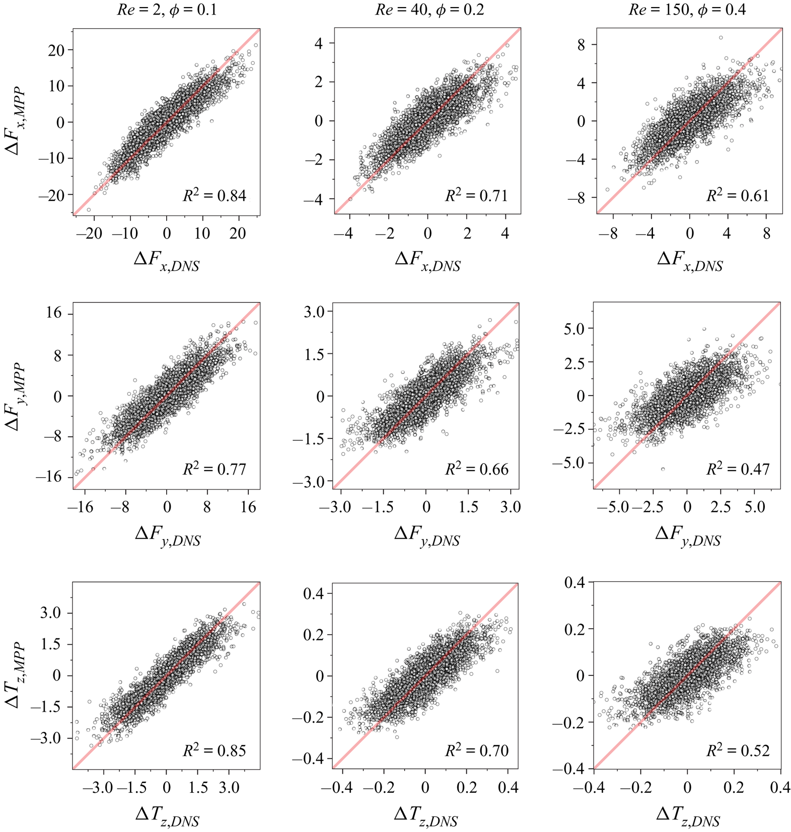
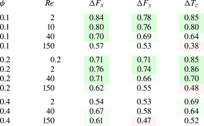
In the present work, we propose a novel data-driven model that relies on force/torque-conditioned probabilities of particle arrangements extracted from PR-DNS in order to correlate hydrodynamic forces and torques to the unique neighbourhood of each particle. In the remainder of this work, we refer to our model as the microstructure-informed probability-driven point-particle (MPP) model. We will provide probabilistic arguments for the prediction of force/torque fluctuations, and apply our method to the data from PR-DNS of fixed beds of randomly distributed spherical particles at various Reynolds numbers and solid volume fractions. After validating our results with the existing literature, we then evaluate the accuracy of our model's predictions and demonstrate its performance by providing comparisons with PR-DNS force and torque data.
2. PR-DNS of fixed beds of spheres
2.1. Governing equations
Conservation of momentum and mass for the fluid phase is expressed in terms of incompressible Navier–Stokes and continuity equations for a Newtonian fluid as follows:
 \begin{gather} \frac{\partial{\boldsymbol{u}}}{\partial{t}} + \boldsymbol{u} \boldsymbol{\cdot} \boldsymbol{\nabla}{\boldsymbol{u}} = -\boldsymbol{\nabla}{p} + \frac{1}{\textit{Re}} \nabla^2 \boldsymbol{u} , \end{gather}
 \begin{gather} \boldsymbol{\nabla}{\boldsymbol{\cdot}}\, \boldsymbol{u} = 0, \end{gather}
where  $\boldsymbol {u}$,
 $p$ and
 $\textit {Re}$ respectively denote the fluid velocity vector, pressure and particle Reynolds number, defined as
 \begin{equation} \textit{Re} = \frac{\rho U d}{\mu} = \frac{\rho (1 - \phi) u_s d}{\mu}, \end{equation}
where  $\rho$,
 $\mu$ are the fluid phase density and dynamic viscosity. The particle Reynolds number is defined based on the superficial velocity
 $U = (1 - \phi ) u_s$, and
 $u_s$ represents the average interstitial fluid velocity. In (2.1) and (2.2) and what follows, all variables are non-dimensionalised with respect to the particle diameter
 $d$ as the length scale,
 $U$ as the velocity scale,
 $\rho U^2$ as the pressure scale and
 $\rho U^2 d^2$ as the force scale. The hydrodynamic force and torque exerted on each particle denoted by
 $\boldsymbol {F}$ and
 $\boldsymbol {T}$ are given as
 \begin{gather} \boldsymbol{F}= \int_{S}\left[ -p\boldsymbol{\mathsf{I}}+\frac{1}{\textit{Re}}(\boldsymbol{\nabla}{\boldsymbol{u}}+\boldsymbol{\nabla}{\boldsymbol{u}^{\textrm{T}}}) \right] \boldsymbol{\cdot} \boldsymbol{n} \,\textrm{d}S, \end{gather}
 \begin{gather} \boldsymbol{T} = \int_{S}\boldsymbol{r}\times\left[ -p\boldsymbol{\mathsf{I}}+\frac{1}{\textit{Re}}(\boldsymbol{\nabla}{\boldsymbol{u}}+\boldsymbol{\nabla}{\boldsymbol{u}^{\textrm{T}}}) \right] \boldsymbol{\cdot} \boldsymbol{n} \,\textrm{d}S, \end{gather}
with  $S$ denoting the surface enclosing the solid body,
 $\boldsymbol{\mathsf{I}}$ the identity matrix,
 $(\cdot )^\textrm {T}$ the matrix transpose,
 $\boldsymbol {n}$ the unit vector normal to the boundary of the solid body and
 $\boldsymbol {r}$ the position vector relative to the particle centre of mass.
2.2. Numerical method
As our PR-DNS tool, we use PeliGRIFF (Parallel Efficient Library for GRains in Fluid Flow) which is a multiphase flow solver based on the distributed Lagrange multiplier-fictitious domain (DLM-FD) formulation proposed by Glowinski et al. (Reference Glowinski, Pan, Hesla and Joseph1999). In our implementation, we employ a finite-volume staggered-grid scheme for the fluid conservation equations (Wachs et al. Reference Wachs, Hammouti, Vinay and Rahmani2015). Similar to the IBM, particles are immersed in the fluid domain in the DLM-FD method and rigid-body constraints on the fictitious fluid inside the solid region are enforced through a set of Lagrange multipliers collocated in the particle domain. For a fixed array of particles, the combined momentum and continuity equations in a non-variational form are given as
 \begin{gather} \frac{\partial{\boldsymbol{u}}}{\partial{t}} + \boldsymbol{u} \boldsymbol{\cdot} \boldsymbol{\nabla}{\boldsymbol{u}} = -\boldsymbol{\nabla}{p} + \frac{1}{\textit{Re}} \nabla^2\boldsymbol{u} - \boldsymbol{\lambda} \quad \text{in} \ \mathbb{D}, \end{gather}
 \begin{gather} \boldsymbol{\nabla}\boldsymbol{\cdot}{\boldsymbol{u}} = 0 \quad\text{in} \ \mathbb{D}, \end{gather}
 \begin{gather} \boldsymbol{u} = \boldsymbol{0} \quad\text{in} \ \mathbb{P}, \end{gather}
where the solid domain is denoted by  $\mathbb {P}$ and the fluid–particle domain by
 $\mathbb {D}$. Furthermore,
 $\boldsymbol {\lambda }$ shows the distributed Lagrange multiplier vector which is used to enforce the rigid-body motion constraint (2.5c). For the temporal discretisation, we employ a first-order Marchuk–Yanenko operator-splitting algorithm. At each time
 $t^{n+1}$, we solve:
(i) A classical projection scheme for the solution of the Navier–Stokes problem: find
 $\boldsymbol {u}^{n+1/2}$ and $p^{n+1}$ such that
(2.6a)\begin{align} &\frac{\tilde{\boldsymbol{u}}^{n+1/2} - \boldsymbol{u}^{n}}{{\rm \Delta} t} - \frac{1}{2 \textit{Re}}\boldsymbol{\nabla}^{2}{\tilde{\boldsymbol{u}}^{n+1/2}}\nonumber\\
&\quad =-{\boldsymbol{\nabla} p^{n}} + \frac{1}{2 \textit{Re}}{\nabla^{2} \boldsymbol{u}^{n}} -\frac{1}{2} \left( 3\boldsymbol{u}^{n}\boldsymbol{\cdot} \boldsymbol{\nabla} \boldsymbol{u}^{n} - \boldsymbol{u}^{n-1}\boldsymbol{\cdot} \boldsymbol{\nabla} \boldsymbol{u}^{n-1} \right) - \boldsymbol{\lambda}^{n},\end{align}(2.6b)\begin{gather} \left.\begin{array}{c@{}} \nabla^{2}{\psi^{n+1}} = \dfrac{1}{{\rm \Delta} t}\boldsymbol{\nabla}\boldsymbol{\cdot}{\tilde{\boldsymbol{u}}^{n+1/2}},\\ \dfrac{\partial{\psi^{n+1}}}{\partial{n}} =0\quad \text{on} \ \partial \mathbb{D}, \end{array}\right\} \end{gather}(2.6c)\begin{gather} \boldsymbol{u}^{n+1/2} = \tilde{\boldsymbol{u}}^{n+1/2} - {\rm \Delta} t \boldsymbol{\nabla}\psi^{n+1}, \end{gather}(2.6d)\begin{gather} p^{n+1} = p^n + \psi^{n+1} - \frac{{\rm \Delta} t}{2 \textit{Re}}\nabla^{2}{\psi^{n+1}}. \end{gather}
(ii) A fictitious domain problem: find
$\boldsymbol {u}^{n+1}$ and $\boldsymbol {\lambda }^{n+1}$ such that
(2.7a)\begin{gather} \frac{\boldsymbol{u}^{n+1}-\boldsymbol{u}^{n+1/2}}{{\rm \Delta} t} +\boldsymbol{\lambda}^{n+1} = \boldsymbol{\lambda}^{n}, \end{gather}(2.7b)\begin{gather} \boldsymbol{u}^{n+1} = \boldsymbol{0} \quad \text{in} \ \mathbb{P}, \end{gather}


where  ${\rm \Delta} t$ denotes the time step,
 $\psi$ the pseudo-pressure and
 $\partial \mathbb {D}$ the domain boundary. In (2.6a), second order in time Crank–Nicolson and Adams–Bashforth schemes are used to discretise the viscous and advective terms, respectively, and the saddle-point problem in step (ii) is handled by an Uzawa algorithm (Wachs et al. Reference Wachs, Hammouti, Vinay and Rahmani2015). Considering the high-order correction of the pressure, the projection scheme in step (i) is also second-order accurate in time. However, the first-order time discretisation of the fictitious domain sub-problem in step (ii) and the first-order Marchuk–Yanenko method reduce the global time accuracy of our algorithm to first order only. Equations presented in step (i) are spatially discretised with a second-order central scheme for the diffusion term, whereas the advective term is treated with a total variation diminishing scheme combined with a Superbee flux limiter. Despite the second-order discretisation of the flow equations, the accuracy of our method is between first and second order due to the presence of rigid bodies immersed within the domain. It can be shown that with the DLM-FD method, the Lagrange multiplier
 $\boldsymbol {\lambda }$ can be directly integrated over the volume of each particle to obtain the hydrodynamic force and torque acting on the particle
 $\mathbb {P}$
 \begin{gather} \boldsymbol{F} = \int_{\mathbb{P}} \boldsymbol{\lambda} \,\textrm{d}\boldsymbol{x}, \end{gather}
 \begin{gather} \boldsymbol{T} = \int_{\mathbb{P}} \boldsymbol{r} \times \boldsymbol{\lambda} \,\textrm{d}\boldsymbol{x}. \end{gather}
2.3. Simulation set-up
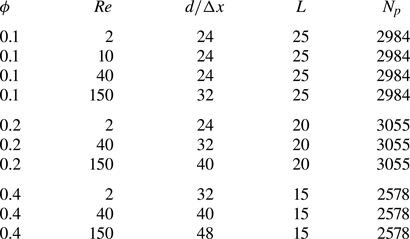
A summary of all considered cases is given in table 1. For our PR-DNS simulations, we consider triply periodic cubic domains of edge length  $L$ containing
 $N_p$ spherical particles each taking up a volume of
 $v_p = \pi / 6$, corresponding to a solid volume fraction of
 $\phi = N v_p/ L^3$. A constant flow rate so as to attain the desired Reynolds number is imposed in the
 $x$ direction using a dynamically adjusted pressure drop. The
 $x$ direction hence corresponds here to the streamwise direction. As noted by Akiki et al. (Reference Akiki, Jackson and Balachandar2016), Tenneti et al. (Reference Tenneti, Garg and Subramaniam2011) demonstrated that using a domain size of only
 $2.4 d$ guarantees the decorrelation of fluid velocities for
 $(\textit {Re}, \phi ) = (20, 0.2)$ and
 $(\textit {Re}, \phi ) = (300, 0.2)$. Our computational domains given in table 1 all extend far beyond
 $2.4 d$ containing
 $\approx$2500–3000 particles each, ensuring both the decay of fluid correlations and statistical reliability. Initialisation of particle locations for cases where
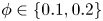 $\phi \in \{0.1, 0.2\}$ is performed by distributing spheres randomly in the domain according to a random number generation algorithm without allowing any overlap. For the highly dense cases with
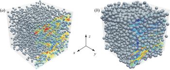
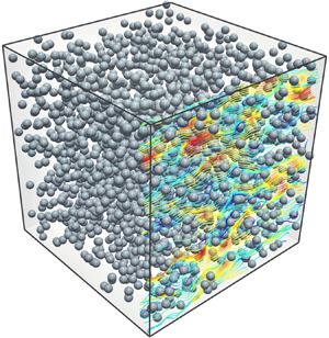
 $\phi = 0.4$, we start with a structured array of particles where each particle is given a random translational and rotational velocity, and we let the system reach an asymptotic motionless state through dissipative collisions. For all solid volume fractions, pair correlation functions have been obtained and verified to be satisfactorily matching theoretical radial distribution functions of hard spheres (Percus & Yevick Reference Percus and Yevick1958; Wertheim Reference Wertheim1963). Visualisations of two sample cases in the present study are shown in figure 2. The time step is taken to be smaller than
 ${\rm \Delta} t = 2 \times 10^{-3}$ in all cases, ensuring time accuracy of the simulations along with satisfying the Courant–Friedrichs–Lewy (CFL) condition; namely,
 $\mathrm {CFL} < 0.4$ for the spatial resolutions presented in table 1. The simulations have been run until steady state is achieved, and force and torque data are all collected from the steady part. For
 $\textit {Re} = 150$ at all volume fractions, the flow becomes time dependent and oscillating. This occurs because particles in close proximity act as a single obstacle and hence increase the effective length scale and the Reynolds number. Data from these cases are collected after a statistically pseudo-stationary state is established by averaging over sufficiently extended time intervals. In terms of computational demand, the mesh resolution and the domain size in each case along with the load per CPU core dictate resource requirements. With each processor core handling
 $512 \times 10^3$ grid cells, the smallest simulations with
 $\approx \! 110 \times 10^6$ grid cells were run on 192 cores, whereas the largest ones with
 $512 \times 10^6$ grid cells required 960 cores. All computations were carried out on groups of 48-core nodes each equipped with
 $\approx$187 GB of memory, provided by the Cedar supercomputer as a part of Compute Canada's advanced research computing infrastructure (http://www.computecanada.ca).
Fixed beds of spherical particles at  $\textit {Re}=40$ and solid volume fractions of
 $\phi = 0.1$ (a) and
 $\phi = 0.4$ (b). The streamlines shown are coloured with respect to the fluid velocity magnitude.

Summary of the parameters used for PR-DNS of fixed beds of spheres.

2.4. Validation
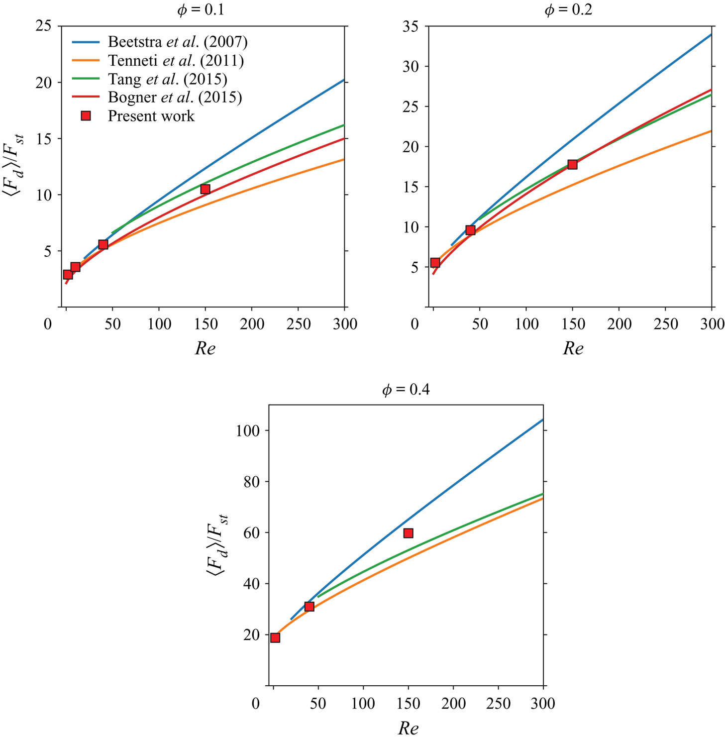
The aim in this section is to provide a comparison of the results of our PR-DNS simulations with the reported drag correlations in the literature (Beetstra et al. Reference Beetstra, van der Hoef and Kuipers2007; Tenneti et al. Reference Tenneti, Garg and Subramaniam2011; Bogner et al. Reference Bogner, Mohanty and Rüde2015; Tang et al. Reference Tang, Peters, Kuipers, Kriebitzsch and van der Hoef2015). In terms of spatial resolution, our PR-DNS is comparable with the work of Bogner et al. (Reference Bogner, Mohanty and Rüde2015) and Tenneti et al. (Reference Tenneti, Garg and Subramaniam2011) for the range of  $(\textit {Re}, \phi )$ considered here, but generally better resolved than simulations done by Tang et al. (Reference Tang, Peters, Kuipers, Kriebitzsch and van der Hoef2015) and Beetstra et al. (Reference Beetstra, van der Hoef and Kuipers2007). Nevertheless, validations are presented merely to establish the accuracy of our code rather than intending to offer benchmarking data. The ensemble-average drag is obtained by summing the drag force acting on each particles in the bed and dividing by the total number of particles
 $N_p$
 \begin{equation} \langle F_d \rangle = \frac{1}{N_p} \sum_{i=1}^{N_p} \boldsymbol{F}_i \boldsymbol{\cdot} \hat {\boldsymbol{e}}_{x}. \end{equation}
Obviously, the normal components of the mean force  $\langle F_y \rangle = \langle \boldsymbol {F} \boldsymbol {\cdot } \hat {\boldsymbol{e}}_{y} \rangle$ and
 $\langle F_z \rangle = \langle \boldsymbol {F} \boldsymbol {\cdot } \hat {\boldsymbol {e}_z} \rangle$ are both expected to be vanishingly small. In order to compare our data with the available drag correlations, normalisation of forces is done with respect to the Stokes drag given as
 \begin{equation} F_{st} = 3 \pi \mu \,\textrm{d} U. \end{equation}
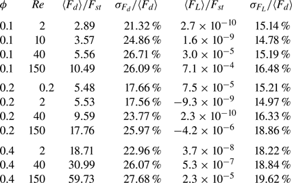
As shown in figure 3, the drag computed for our cases listed in table 1 all lie within the range of existing correlations and generally indicate good accordance. In particular, our data seem to agree well with correlations proposed by Bogner et al. (Reference Bogner, Mohanty and Rüde2015) and Tang et al. (Reference Tang, Lau, Deen, Peters and Kuipers2016) at  $\textit {Re} = 150$ where significant discrepancies are observed between different correlations. In addition, we have also examined force distributions and the extent of data scatter for each case in table 2. The magnitude of the ensemble-average lift force given as
 $\langle F_L \rangle = \langle F_y \rangle$ or
 $\langle F_z \rangle$ is practically zero for all cases, as expected. However, the ratio of the standard deviation of drag and lift shown by
 $\sigma _{F_d}/\langle F_d \rangle$ and
 $\sigma _{F_L}/\langle F_d \rangle$ are both significant and
 $\sigma _{F_d}/\langle F_d \rangle$ turns out to be always greater than
 $\sigma _{F_L}/\langle F_d \rangle$. In cases where a rough comparison is possible, our results for
 $\sigma _{F_d}/\langle F_d \rangle$ and
 $\sigma _{F_L}/\langle F_d \rangle$ in table 2 show a difference of
 $\approx$2 %–4 % with those obtained by Akiki et al. (Reference Akiki, Jackson and Balachandar2016). A contributing feature that might explain the difference is that our sample sizes for each case are significantly larger by a factor of
 $5\hbox{--}6$, rendering the results statistically more converged. This is obvious from the
 $\langle F_L \rangle$ values in table 2 compared with those reported by Akiki et al. (Reference Akiki, Jackson and Balachandar2016), as their mean lift data (while still quite close to zero) are orders of magnitude greater than present results. According to Akiki et al. (Reference Akiki, Jackson and Balachandar2016), realisation dependence alone could cause variance in
 $\sigma _{F_d}/\langle F_d \rangle$ and
 $\sigma _{F_L}/\langle F_d \rangle$ of up to
 $2.7\,\%$ and
 $1.7\,\%$, respectively.
Validation of the drag data obtained from PR-DNS of the present work with correlations of Beetstra et al. (Reference Beetstra, van der Hoef and Kuipers2007), Tenneti et al. (Reference Tenneti, Garg and Subramaniam2011), Tang et al. (Reference Tang, Peters, Kuipers, Kriebitzsch and van der Hoef2015) and Bogner et al. (Reference Bogner, Mohanty and Rüde2015).

Statistics of the drag and lift data for cases presented in table 1.

2.5. Dataset construction
For the purpose of analysis and development of our model, we first need to construct datasets corresponding to each simulation. Each dataset contains as many rows as the number of particles  $N_p$ (which we call samples), while columns represent the input and output variables. For each particle
 $i$, the set of position vectors of the neighbouring spheres denoted by
 $\{ \boldsymbol {r}_{j=1}, \ldots , \boldsymbol {r}_{j=M} \}$ along with the average fluid velocity
 $\overline {\boldsymbol {u}}_i$ around particle
 $i$ constitute the inputs, whereas the hydrodynamic forces and torques experienced by particle
 $i$ are the outputs that we aim to model. The position vectors of neighbours are expressed relative to the location of particle
 $i$. The first
 $30$ nearest neighbours are identified for each particle
 $i$ by looping over all other particles in the simulation. These neighbours are then numbered from
 $j=1$ to
 $j=30$ depending on their relative distance, with
 $j=1$ being the closest. It is worthwhile noting that, since our simulations are performed in tri-periodic domains, forces and torques on particles near boundaries could be affected by periodic images of particles on the opposite side of the domain whose positions do not exist in the simulation data. For this reason, prior to performing the neighbour identification loop, we create the periodic image positions manually and explicitly insert them in the data so that the periodic effects are correctly accounted for.
3. Probability-driven model
3.1. Motivation
As pointed out in § 1, we seek to predict the hydrodynamic forces and torques on each particle as a function of the flow conditions, and more importantly, of the unique neighbourhood of each particle as highlighted by (1.2). The hydrodynamic force and torque exerted on each sphere may be decomposed and expressed as follows:
 \begin{gather} \boldsymbol{F}_i = \langle \boldsymbol{F}_i \rangle (\textit{Re}, \phi) + {\rm \Delta} \boldsymbol{F}_i(\textit{Re}, \phi, \{ \boldsymbol{r}_{j=1}, \ldots, \boldsymbol{r}_{j=M} \}), \end{gather}
 \begin{gather} \boldsymbol{T}_i = {\rm \Delta} \boldsymbol{T}_i(\textit{Re}, \phi, \{ \boldsymbol{r}_{j=1}, \ldots, \boldsymbol{r}_{j=M} \}), \end{gather}
where  ${\rm \Delta} \boldsymbol {F}_i$ and
 ${\rm \Delta} \boldsymbol {T}_i$ show the fluctuating contribution to the force and torque due to the specific arrangement of neighbours surrounding particle
 $i$. Statistically, the lateral components of
 $\langle \boldsymbol {F}_i \rangle$ and all components of
 $\langle \boldsymbol {T}_i \rangle$ are close to zero for a sufficiently large number of particles in each simulation. In the streamwise direction, the ensemble-average force
 $\langle \boldsymbol {F}_i \rangle$ is identical for all particles by definition and therefore only depends on macroscopic variables, i.e. the Reynolds number and solid volume fraction. Many correlations exist that describe such a dependence as discussed in § 1. For this reason, we henceforth focus on
 ${\rm \Delta} \boldsymbol {F}_i$ and
 ${\rm \Delta} \boldsymbol {T}_i$ in (3.1); namely, the deviations from the mean arising due to the unique local neighbourhood of each particle.
The key question posed here may be expressed as follows: How does changing the location of each neighbour affect the force and torque experienced by a particle? The most obvious and naive strategy would be attempting multiple simulations where the location of a single neighbour particle is changed systematically and the resulting effect on forces and torques are recorded. The outcome would be similar to, for example, the two-dimensional interaction maps given by Zhou & Alam (Reference Zhou and Alam2016) for two neighbouring cylinders characterising forces for various locations of a second cylinder. Assuming a three-dimensional system, adding only one or two more neighbours to the scenario makes the number of simulations needed for populating the modelling dataset an almost intractable computational task. For their physics-based PIEP model, Akiki et al. (Reference Akiki, Jackson and Balachandar2017a) needed to account for 15–40 closest neighbours to obtain good accuracy, which in three dimensions translates into 45–120 input variables, respectively. It is well known that in a data-driven framework, such systems are afflicted with the ‘curse of dimensionality’ (Hastie, Tibshirani & Friedman Reference Hastie, Tibshirani and Friedman2009). It means that constructing a reliable dataset for a regression-type model requires millions of samples for each case, while we are only able to model a few thousand particles with PR-DNS at best. The pairwise interactions and order-invariance approximations utilised by Moore et al. (Reference Moore, Balachandar and Akiki2019) for their data-driven model is a good demonstration of a strategy for reducing the number of input variables to a manageable level.
3.2. Theory
Consider a monodisperse random array of spherical particles with a volume fraction  $\phi$ subject to fluid flow with a Reynolds number
 $\textit {Re}$. Let
 $\boldsymbol {X}$ and
 $\boldsymbol {Y}$ be two continuous random variable vectors in a
 $d$-dimensional space (
 $\boldsymbol {X}, \boldsymbol {Y} \in \boldsymbol {R}^d$) with marginal probability density functions (PDFs)
 $f_{\boldsymbol {X}}(\boldsymbol {x})$ and
 $f_{\boldsymbol {Y}}(\boldsymbol {y})$ where
 $f_{\boldsymbol {X}}(\boldsymbol {x}), f_{\boldsymbol {Y}}(\boldsymbol {Y}) : \boldsymbol {R}^d \rightarrow \boldsymbol {R}$. By definition, PDFs in general are required to satisfy the following conditions:
 \begin{equation} \left.\begin{array}{c@{}} f_{\boldsymbol{X}}(\boldsymbol{x}) \geq 0,\\ \displaystyle\int f_{\boldsymbol{X}}(\boldsymbol{x}) \,\textrm{d}\boldsymbol{x} = 1, \end{array}\right\} \end{equation}
where the integration is performed on all possible values of  $\boldsymbol {x}$. The value
 $f_{\boldsymbol {X}}(\boldsymbol {x}) \,\textrm {d}\boldsymbol {x}$ represents the probability of
 $\boldsymbol {X}$ falling in the infinitesimal volume
 $\textrm {d}\boldsymbol {x}$ about
 $\boldsymbol {x}$. Therefore, the probability that the random variable
 $\boldsymbol {X}$ will happen to be in
 $\mathcal {A}$ is given by
 \begin{equation} P \left[ \boldsymbol{X} \in \mathcal{A} \right] = \int_{ \mathcal{A} } f_{\boldsymbol{X}}(\boldsymbol{x}) \,\textrm{d}\boldsymbol{x}. \end{equation}
The same properties similarly hold for  $f_{\boldsymbol {Y}}(\boldsymbol {y})$. The expected value of the random variable
 $\boldsymbol {X}$ is the weighted average of all possible values of
 $\boldsymbol {X}$, each value being weighted according to its probability of occurrence (Ross Reference Ross2010). The expected value of
 $\boldsymbol {X}$ is thus governed by its probability density distribution
 $f_{\boldsymbol {X}}(\boldsymbol {x})$, and is given as
 \begin{equation} E \left[ \boldsymbol{X} \right] = \langle \boldsymbol{X} \rangle = \int \boldsymbol{x} f_{\boldsymbol{X}}(\boldsymbol{x}) \,\textrm{d}\boldsymbol{x}. \end{equation}
The probability associated with a random variable may also be conditioned on another random variable. For this case,  $f_{\boldsymbol {X} \mid \boldsymbol {Y}}(\boldsymbol {x} \mid \boldsymbol {y})$ may be defined as the conditional PDF of
 $\boldsymbol {X}$ given that
 $\boldsymbol {Y}$ assumes a particular fixed value
 $\boldsymbol {y}$.
 \begin{equation} E \left[\boldsymbol{X} \: \vert \: \boldsymbol{Y}=\boldsymbol{y} \right] = \langle \boldsymbol{X} \mid \boldsymbol{Y}=\boldsymbol{y} \rangle = \int \boldsymbol{x} f_{\boldsymbol{x} \mid \boldsymbol{y}} \left(\boldsymbol{x} \: \vert \: \boldsymbol{y} \right)\,\textrm{d}\boldsymbol{x}. \end{equation}
Referring to (3.1), the three components of the force/torque fluctuations pertaining to particle  $i$ are shown by
 ${\rm \Delta} \boldsymbol {F}_i = \left ({\rm \Delta} F_{i,x}, {\rm \Delta} F_{i,y} , {\rm \Delta} F_{i,z}\right ) ^\textrm {T}$ or
 ${\rm \Delta} \boldsymbol {T}_i = \left ({\rm \Delta} T_{i,x}, {\rm \Delta} T_{i,y} , {\rm \Delta} T_{i,z}\right ) ^\textrm {T}$. A particular configuration of the neighbourhood surrounding particle
 $i$ is denoted by
 $\boldsymbol {R}_i = \{ \boldsymbol {r}_{j=1}, \ldots , \boldsymbol {r}_{j=M} \}$. Here, we present the analysis only for force fluctuations; namely,
 ${\rm \Delta} \boldsymbol {F}$, since the derivation of similar equations is similarly done for torque fluctuations
 ${\rm \Delta} \boldsymbol {T}$. From this point onwards, the subscript
 $i$ is dropped from all variables in order to minimise cluttering in the notations. Upon setting
 $\boldsymbol {X} = {\rm \Delta} F$ and
 $\boldsymbol {Y} = \boldsymbol {R}$, the following PDF
 \begin{equation} p_{{\rm \Delta} F \mid \boldsymbol{R}} \left({\rm \Delta} F \: \vert \: \boldsymbol{R} \right) \end{equation}
represents the probability distribution of the force/torque fluctuations given the locations of  $M$ neighbours. In the above equations,
 $\boldsymbol {R}$ shows the set of position vectors
 $\{\boldsymbol {r}_1, \boldsymbol {r}_2, \boldsymbol {r}_3, \ldots , \boldsymbol {r}_M \}$ belonging to the neighbours numbered according to their distance from a reference particle, starting with
 $j=1$ being the closest. Each distribution
 $p \left ({\rm \Delta} F \: \vert \: \boldsymbol {R} \right )$ is to be obtained from collecting
 ${\rm \Delta} F$ values experienced by particles that happen to have the same neighbour configuration
 $\boldsymbol {R}$, while no constraints are imposed on neighbours
 $\{ \boldsymbol {r}_j : j > M \}$ located further away. The expected value of the PDF in (3.6) gives a prediction of each fluctuating force/torque component as follows:
 \begin{equation} E \left[{\rm \Delta} F \: \vert \: \boldsymbol{R} \right] = \langle {\rm \Delta} F \mid \boldsymbol{R} \rangle = \int \xi p_{{\rm \Delta} F \mid \boldsymbol{R}} \left({\rm \Delta} F \: \vert \: \boldsymbol{R} \right) \,\textrm{d} \xi . \end{equation}
Two extreme cases of  $M$, the number of included neighbours, are worth elaborating on.
(a)
$M=0$: this means that no conditions are imposed on $p$, hence $E[{\rm \Delta} F] = 0$ and the predicted force/torque is the same for all particles in the array. Such a situation corresponds to, for instance, the conventional microstructure-ignorant correlations of the form $\boldsymbol {F} \cdot \hat {\boldsymbol {e}_x} = \langle F_x \rangle (\textit {Re}, \phi )$ in case of the drag force.(b)
$M \to N_p-1$: the positions of all neighbours in the particle array are imposed as a condition on $p$, hence the variance of $p$ tends to zero and the value of ${\rm \Delta} F$ is uniquely determined.


Since the problem is fully constrained in the latter case, the predicted value of  ${\rm \Delta} F$ would be free of uncertainty. Put another way,
 $p$ would no longer be a distribution per se, but rather resembles a Dirac delta function instead:
 \begin{equation} \lim_{M \to N_{p-1}} E \left[{\rm \Delta} F \: \vert \: \boldsymbol{R} \right] = \int_{-\infty}^{+\infty} \xi \delta_{{\rm \Delta} F \mid \boldsymbol{R}} \left( \xi - {\rm \Delta} F_{\textit{DNS}} \: \vert \: \boldsymbol{R} \right) \,\textrm{d} \xi = {\rm \Delta} F_{\textit{DNS}}, \end{equation}
which is equivalent of having a dataset populated with an infinite number of samples. In other words, this ‘ideal’ dataset would contain samples for each and every combination of neighbour locations. Such a dataset would conceivably provide a full and exact description of the problem, thus representing a solution to the Navier–Stokes equations. Consequently, (3.6) can be viewed as a data-driven description of forces/torques exerted on each particle within an array derived from probabilistic arguments, which is potentially capable of predicting fluctuations with varying degrees of accuracy, depending on how constrained we force  $p$ to be. It is crucial to realise that unless
 $M = N_p - 1$, our best estimate of the fluctuating component
 $E \left [{\rm \Delta} F \: \vert \: \boldsymbol {R} \right ]$ would be an average (i.e. the central tendency) of the distribution, implying that for
 $M < N_p-1$, influence of neighbours whose positions are not constrained is only accounted for in a statistical sense. Having established the notion and properties of the conditioned force/torque PDFs, the probability-driven prediction of a fluctuating component based on its corresponding distribution is given as
 \begin{equation} {\rm \Delta} F_{\textit{MPP}} = E \left[{\rm \Delta} F \: \vert \: \boldsymbol{R} \right] = \int_{-\infty}^{+\infty} \xi p_{{\rm \Delta} F \mid \boldsymbol{R}} \left( \xi \: \vert \: \boldsymbol{R} \right) \,\textrm{d} \xi . \end{equation}
The integral above may be split to cover the positive and negative force/torque contributions separately, yielding
 \begin{equation} {\rm \Delta} F_{\textit{MPP}} = \int_{-\infty}^{0} \xi p_{{\rm \Delta} F \mid \boldsymbol{R}} \left( \xi \: \vert \: \boldsymbol{R} \right) \,\textrm{d} \xi + \int_{0}^{+\infty} \xi p_{{\rm \Delta} F \mid \boldsymbol{R}} \left( \xi \: \vert \: \boldsymbol{R} \right) \,\textrm{d} \xi . \end{equation}
The impeding hurdle with (3.10) is that computing  ${\rm \Delta} F_{\textit{MPP}}$ requires a priori knowledge of the force/torque distributions for each and every possible configuration
 $\boldsymbol {R}$. Such an approach is clearly not feasible and certainly would not fulfil the goal of constructing a model based on a limited dataset. An elegant alternative is to take advantage of Bayes’ theorem for probabilities, which serves to convert a conditional probability problem to its reverse case. According to the Bayes’ formula for distributions of random variables (Papoulis, Pillai & Pillai Reference Papoulis, Pillai and Pillai2002),
 $f_{\boldsymbol {X} | \boldsymbol {Y}}(\boldsymbol {x} \mid \boldsymbol {y}) = f_{\boldsymbol {Y} | \boldsymbol {X}}(\boldsymbol {y} \mid \boldsymbol {x}) f_{\boldsymbol {X}}(\boldsymbol {x}) / f_{\boldsymbol {Y}}(\boldsymbol {y})$. Therefore, it follows that
 \begin{equation} p_{{\rm \Delta} F \mid \boldsymbol{R}} \left({\rm \Delta} F \: \vert \: \boldsymbol{R} \right) = \frac{ p_{\boldsymbol{R} \mid {\rm \Delta} F} \left( \boldsymbol{R} \: \vert \: {\rm \Delta} F \right) p_{{\rm \Delta} F}\left({\rm \Delta} F \right) }{ p_{\boldsymbol{R}}\left( \boldsymbol{R} \right) }. \end{equation}
Substituting for  $p_{{\rm \Delta} F \mid \boldsymbol {R}} \left ( \xi \: \vert \: \boldsymbol {R} \right )$ in first integral in (3.10) yields
 \begin{equation} \frac{1}{p_{\boldsymbol{R}}\left( \boldsymbol{R} \right)} \int_{-\infty}^{0} \xi p_{\boldsymbol{R} \mid {\rm \Delta} F} \left( \boldsymbol{R} \: \vert \: \xi \right) p_{{\rm \Delta} F}\left( \xi \right) \textrm{d} \xi . \end{equation}
Assuming the continuity of both  $p_{\boldsymbol {R} \mid {\rm \Delta} F}$ and
 $p_{{\rm \Delta} F}$ and realising that
 $p_{\boldsymbol {R} \mid {\rm \Delta} F} , p_{{\rm \Delta} F} \geq 0$, the generalised mean value theorem for integrals can be applied to the above equation to give
 \begin{equation} \frac{\alpha p_{{\rm \Delta} F}(\alpha) }{p_{\boldsymbol{R}}\left( \boldsymbol{R} \right)} \int_{-\infty}^{0} p_{\boldsymbol{R} \mid {\rm \Delta} F} \left( \boldsymbol{R} \: \vert \: \xi \right) \,\textrm{d} \xi = \left[ \frac{\alpha p_{{\rm \Delta} F}(\alpha) }{p_{\boldsymbol{R}}\left( \boldsymbol{R} \right)} \right] p_{\boldsymbol{R} \mid {\rm \Delta} F} \left( \boldsymbol{R} \: \vert \: {\rm \Delta} F < 0 \right), \end{equation}
where  $\xi = \alpha$ is a constant value that belongs to the interval
 $(-\infty , 0]$. Following the same operations for the second integral of (3.10), there exists a value
 $\xi = \beta$ in
 $[0, +\infty )$ for which
 $\xi p_{{\rm \Delta} F}( \xi )$ can be brought out of the integral. Substituting results back in (3.10), we arrive at the following:
 \begin{equation} {\rm \Delta} F_{\textit{MPP}} = \left[ \frac{\alpha p_{{\rm \Delta} F}(\alpha) }{p_{\boldsymbol{R}}\left( \boldsymbol{R} \right)} \right] p_{\boldsymbol{R} \mid {\rm \Delta} F} \left( \boldsymbol{R} \: \vert \: {\rm \Delta} F < 0 \right) + \left[ \frac{\beta p_{{\rm \Delta} F}(\beta) }{p_{\boldsymbol{R}}\left( \boldsymbol{R} \right)} \right] p_{\boldsymbol{R} \mid {\rm \Delta} F} \left( \boldsymbol{R} \: \vert \: {\rm \Delta} F > 0 \right). \end{equation}
Note that, according to (3.5),  $p_{\boldsymbol {R} \mid {\rm \Delta} F} \left ( \boldsymbol {R} \: \vert \: {\rm \Delta} F < 0 \right )$ gives the PDF of particle positions provided that the force/torque fluctuations obey
 ${\rm \Delta} F < 0$ (same applies to
 $p_{\boldsymbol {R} \mid {\rm \Delta} F} \left ( \boldsymbol {R} \: \vert \: {\rm \Delta} F > 0 \right )$ when
 ${\rm \Delta} F > 0$). Since particles are assumed to be randomly, yet uniformly distributed,
 $p_{\boldsymbol {R}}( \boldsymbol {R} )$ is expected to have an approximately constant distribution. This can be verified by inspection of unconditioned particle location PDFs for various neighbours. Therefore, both terms inside the square brackets in (3.14) are constant values and can be expressed as two coefficients
 $c_{\alpha }$ and
 $c_{\beta }$. The final form of the force/torque model reads
 \begin{equation} {\rm \Delta} F_{\textit{MPP}}(\boldsymbol{R}, \textit{Re}, \phi) = c_{\alpha}\,\tilde{p} \left(\boldsymbol{R} \: \vert \: {\rm \Delta} F < 0 \right) + c_{\beta}\,\tilde{p} \left(\boldsymbol{R} \: \vert \: {\rm \Delta} F > 0 \right), \end{equation}
where  $\tilde {p}$ represents the conditional PDF
 $p_{\boldsymbol {R} \mid {\rm \Delta} F}$. It should be noted that the
 $\tilde {p}$ probability maps depend on the Reynolds number and solid volume fraction, which is why
 ${\rm \Delta} F_{\textit{MPP}}$ is shown as
 ${\rm \Delta} F_{\textit{MPP}}(\boldsymbol {R}, \textit {Re}, \phi )$. Thus far, no approximation was involved in the derivation of
 ${\rm \Delta} F_{\textit{MPP}}$, which means that in case a full knowledge of the aforementioned distributions exists, (3.15) would be theoretically exact. Practically, however, for a dataset with a few thousand samples the probability distributions
 $\tilde {p} \left (\boldsymbol {R} \: \vert \: {\rm \Delta} F < 0 \right )$ or
 $\tilde {p} \left (\boldsymbol {R} \: \vert \: {\rm \Delta} F > 0 \right )$ would be extremely sparse, as alluded to in § 3.1. Taking
 $N$ and
 $D$ to denote sample size and number of input dimensions, the data density would be proportional to
 $N^{1/D}$. As
 $D$ increases, it is straightforward to see that maintaining a constant sample density requires exponentially more data points. In our case, each neighbour adds three inputs to the problem, each representing one component of the position vector
 $\boldsymbol {r}_j = (x_j, y_j, z_j)$. If, for instance,
 $N_1 = 1000$ is deemed a sufficiently dense dataset to form reliable local averages when
 $D_1 = M \times 3 = 1 \times 3$ (i.e. a single neighbour considered), in case of 15 neighbours
 $D_2 = 15 \times 3 = 45$, thus
 $N_2 = N_1^{(D_2/D_1)} = 1000^{15}$. Ordinary PR-DNS-generated simulations of particle arrays are far from being sufficiently dense for creating meaningful, reliable functional forms for
 $\tilde {p}$. As a result, the curse of dimensionality precludes the construction of PDFs in (3.15) in their current form. Any such effort is in fact bound to produce a severely over-fitted model with almost no generalisable prediction capability. Consequently, instead of attempting to obtain
 $\tilde {p} \left (\boldsymbol {R} \: \vert \: {\rm \Delta} F < 0 \right )$ and
 $\tilde {p} \left (\boldsymbol {R} \: \vert \: {\rm \Delta} F > 0 \right )$ directly, we suggest that
 \begin{equation}
\left.\begin{array}{c@{}} \tilde{p} \left(\boldsymbol{R} \:
\vert \: {\rm \Delta} F < 0 \right) \approx c_{\alpha, 1}\,\tilde{p}_1 \left(\boldsymbol{r}_1 \: \vert \: {\rm \Delta} F <
0 \right) + c_{\alpha, 2}\,\tilde{p}_2
\left(\boldsymbol{r}_2 \: \vert \: {\rm \Delta} F < 0 \right) +
\cdots \\ = \displaystyle \sum_{j=1}^M c_{\alpha, j} \, \tilde{p}_j
\left(\boldsymbol{r}_j \: \vert \: {\rm \Delta} F < 0 \right),\\
\tilde{p} \left(\boldsymbol{R} \: \vert \: {\rm \Delta} F > 0
\right) \approx c_{\beta, 1}\,\tilde{p}_1
\left(\boldsymbol{r}_1 \: \vert \: {\rm \Delta} F > 0 \right) +
c_{\beta, 2}\,\tilde{p}_2 \left(\boldsymbol{r}_2 \: \vert \:
{\rm \Delta} F > 0 \right) + \cdots\\ = \displaystyle \sum_{j=1}^M c_{\beta,
j} \, \tilde{p}_j \left(\boldsymbol{r}_j \: \vert \: {\rm \Delta} F
> 0 \right). \end{array}\right\}
\end{equation}
In the above equation, each function  $\tilde {p}_j \left (\boldsymbol {r}_j \: \vert \: \cdot \right )$ is equivalent to a marginal probability distribution which is obtained by integrating out the position
 $\boldsymbol {r}_k$ of each and every neighbour where
 $k \ne j$ in
 $\tilde {p} \left (\boldsymbol {R} = \{ \boldsymbol {r}_{k=1}, \ldots , \boldsymbol {r}_{k=M} \} \: \vert \: \cdot \right )$. In other words, this approximation only considers the effect of a single neighbour on the functional form of
 $\tilde {p}$, while accounting for the presence of all other surrounding particles in an average manner. This marginal distribution can be expressed as
 \begin{equation} \tilde{p}_j \left(\boldsymbol{r}_j \: \vert \: \cdot \right) = \int \tilde{p} \left(\boldsymbol{R} \: \vert \: \cdot \right) \,\textrm{d}\boldsymbol{r}_1 \ldots \textrm{d}\boldsymbol{r}_{j-1}\,\textrm{d}\boldsymbol{r}_{j+1} \ldots \textrm{d}\boldsymbol{r}_M. \end{equation}
Equation (3.16) is reminiscent of the pairwise approximation employed by Moore et al. (Reference Moore, Balachandar and Akiki2019) for the purpose of reducing the number of independent variables by accounting for the influence of only one neighbour at a time. In their data-driven model, the authors also invoked the ‘order-invariance’ approximation, which removes the dependence of the model functions on the neighbour number. This was done by weighting the functionals according to the probability of a particular neighbour being the  $j$th closest neighbour. In the MPP model, the neighbours first need to be sorted based on their distance to the reference particle. Each neighbour's position can be then passed to the appropriate PDF.
Substitution of (3.16) in (3.15) leads to
 \begin{equation} {\rm \Delta} F_{\textit{MPP}}(\boldsymbol{R}, \textit{Re}, \phi) = \sum_{j=1}^M c_{\alpha, j} \, \tilde{p}_j \left(\boldsymbol{r}_j \: \vert \: {\rm \Delta} F < 0 \right) + \sum_{j=1}^M c_{\beta, j} \, \tilde{p}_j \left(\boldsymbol{r}_j \: \vert \: {\rm \Delta} F > 0 \right). \end{equation}
In (3.18),  $c_{\alpha , j}$ and
 $c_{\beta , j}$ are constant unknown coefficients. With the final form of
 ${\rm \Delta} F_{\textit{MPP}}$, we have assumed an additive nature for the effect that each neighbour might have on the force/torque fluctuation experienced by a reference particle. Notably, both distributions
 $\tilde {p}_j \left (\boldsymbol {r}_j \: \vert \: \cdot \right )$ (this notation is used to refer to a PDF with any arbitrary force/torque conditioning) are now functions of three variables only; that is, the three components of the position vector
 $\boldsymbol {r}_j = (r_{j,x}, r_{j,y}, r_{j,z})$. This means that the functional form of the PDFs in (3.18) can be conveniently inferred with a data-driven approach, as the high-dimensionality of the input space has been evaded. To this end, a dataset can be constructed by running PR-DNS of fixed beds for desired sets of parameters. The discrete estimation of the distribution
 $\tilde {p}_j$ can be extracted by filtering neighbour positions according to the conditions
 $\{ {\rm \Delta} F < 0, {\rm \Delta} F > 0\}$. The discrete form of the distribution is then fitted with a multivariate kernel density estimation (KDE) function (Chacón & Duong Reference Chacón and Duong2018) of the form
 \begin{equation} \tilde{p} \left(\boldsymbol{r} \: \vert \: \cdot \right) = \frac{1}{m} \sum_{q=1}^{m} K_{\boldsymbol{\mathsf{H}}}(\boldsymbol{r} - \boldsymbol{r}_q), \end{equation}
where
 \begin{equation} K_{\boldsymbol{\mathsf{H}}}(\boldsymbol{r}) = {|\boldsymbol{\mathsf{H}}|}^{-1/2} K(\boldsymbol{\mathsf{H}}^{-1/2} \boldsymbol{r}). \end{equation}
In the above equations,  $m$ shows the total number of samples after filtering with the aforementioned conditions,
 $\boldsymbol{\mathsf{H}}$ the bandwidth matrix and
 $K$ is a symmetric density function of choice. We select a Gaussian distribution as the kernel function defined as
 \begin{equation} K(\boldsymbol{r}) = \frac{1}{(2 \pi)^{D/2}} \exp \left\{ -\frac{1}{2} \boldsymbol{r}^{\textrm{T}} \boldsymbol{r} \right\}. \end{equation}
We will demonstrate and discuss particular examples of these functions in § 3.3. Now that the appropriate functional forms are identified and known, it remains to decide the values of the constant coefficients  $c_{\alpha , j}$ and
 $c_{\beta , j}$ in (3.18). The values are obtained using the ordinary least-squares method for linear regression
 \begin{equation} \{ c_{\alpha, j}, c_{\beta, j} \}_{j=1}^{M} = \text{argmin} \sum_{i=1}^{N_p} \left( {\rm \Delta} F_{\textit{MPP}, i} - {\rm \Delta} F_{\textit{DNS}, i} \right)^{2}, \end{equation}
which minimises the residual sum of squares between values of force/torque fluctuations predicted by the MPP model and the true values from PR-DNS. After optimal values for  $c_{\alpha , j}$ and
 $c_{\beta , j}$ are found, (3.18) can be used to make predictions for each particle based on the particular microstructure of the surrounding particles. It is of great importance to realise that in the presented approach, the model relies solely on the unique configuration of neighbours surrounding each particle, and the PR-DNS-generated force/torque data (as opposed to velocity and pressure fields) in order to make predictions. Consequently, the MPP model accounts for the combined effect of various force contributions such as the undisturbed flow, quasi-steady and added-mass forces. This can be contrasted with the PIEP physics-driven model (Akiki et al. Reference Akiki, Jackson and Balachandar2017a) which uses perturbed velocity and pressure fields together with the Faxén's theorem to obtain hydrodynamic forces experienced by each particle.
The above analysis applies identically to all force and torque fluctuation components; namely,  $\left ({\rm \Delta} F_{x}, {\rm \Delta} F_{y} , {\rm \Delta} F_{z}\right )$ and
 $\left ({\rm \Delta} T_{x}, {\rm \Delta} T_{y} , {\rm \Delta} T_{z}\right )$. Let
 $\boldsymbol {C}_{\alpha }$ denote a
 $1 \times M$ vector that contains the
 $c_{\alpha , j}$ coefficients in (3.18)
 \begin{equation} \boldsymbol{C}_{\alpha} =\begin{pmatrix} c_{\alpha, 1} & \cdots & c_{\alpha, j} & \cdots & c_{\alpha, M} \end{pmatrix} \end{equation}
and let  $\boldsymbol {P}_{{\rm \Delta} F < 0}$ denote an
 $M \times 1$ vector that contains the PDFs
 $\tilde {p}_j \left (\boldsymbol {r}_j \: \vert \: {\rm \Delta} F < 0 \right )$ in (3.18)
 \begin{equation} \boldsymbol{P}_{{\rm \Delta} F < 0} =\begin{pmatrix} \tilde{p}_1 \left(\boldsymbol{r}_1 \: \vert \: {\rm \Delta} F < 0 \right) \\ \vdots \\ \tilde{p}_j \left(\boldsymbol{r}_j \: \vert \: {\rm \Delta} F < 0 \right) \\ \vdots \\ \,\tilde{p}_M \left(\boldsymbol{r}_M \: \vert \: {\rm \Delta} F < 0 \right) \end{pmatrix}. \end{equation}
Together with their counter-parts, i.e.  $\boldsymbol {C}_{\beta }$ and
 $\boldsymbol {P}_{{\rm \Delta} F > 0}$, the above vectors can be ultimately defined for all force components. The complete model equations for force fluctuations can thus be expressed in the following form:
 \begin{equation} {\rm \Delta}
\boldsymbol{F}_{\textit{MPP}}(\boldsymbol{R}, \textit{Re},
\phi) =\begin{pmatrix} {\rm \Delta} F_x \\ {\rm \Delta} F_y \\
{\rm \Delta} F_z \end{pmatrix}=\begin{pmatrix}
\boldsymbol{C}^x_{\alpha} \boldsymbol{P}_{{\rm \Delta} F_x < 0}
+ \boldsymbol{C}^x_{\beta} \boldsymbol{P}_{{\rm \Delta} F_x > 0}
\\ \boldsymbol{C}^y_{\alpha} \boldsymbol{P}_{{\rm \Delta} F_y <
0} + \boldsymbol{C}^y_{\beta} \boldsymbol{P}_{{\rm \Delta} F_y >
0} \\ \boldsymbol{C}^z_{\alpha} \boldsymbol{P}_{{\rm \Delta} F_z
< 0} + \boldsymbol{C}^z_{\beta} \boldsymbol{P}_{{\rm \Delta} F_z
> 0} \end{pmatrix}, \end{equation}
where the superscripts of the coefficients indicate the corresponding component. Following the above definitions, torque fluctuations are given as
 \begin{equation} {\rm \Delta}
\boldsymbol{T}_{\textit{MPP}}(\boldsymbol{R}, \textit{Re},
\phi) =\begin{pmatrix} {\rm \Delta} T_x \\ {\rm \Delta} T_y \\
{\rm \Delta} T_z \end{pmatrix}=\begin{pmatrix}
\boldsymbol{D}^x_{\alpha} \boldsymbol{P}_{{\rm \Delta} T_x < 0}
+ \boldsymbol{D}^x_{\beta} \boldsymbol{P}_{{\rm \Delta} T_x > 0}
\\ \boldsymbol{D}^y_{\alpha} \boldsymbol{P}_{{\rm \Delta} T_y <
0} + \boldsymbol{D}^y_{\beta} \boldsymbol{P}_{{\rm \Delta} T_y >
0} \\ \boldsymbol{D}^z_{\alpha} \boldsymbol{P}_{{\rm \Delta} T_z
< 0} + \boldsymbol{D}^z_{\beta} \boldsymbol{P}_{{\rm \Delta} T_z
> 0} \end{pmatrix}, \end{equation}
where  $\boldsymbol {D}_{\alpha }$,
 $\boldsymbol {D}_{\beta }$,
 $\boldsymbol {P}_{{\rm \Delta} T > 0}$ and
 $\boldsymbol {P}_{{\rm \Delta} T < 0}$ for each torque component are equivalent to
 $\boldsymbol {C}_{\alpha }$,
 $\boldsymbol {C}_{\beta }$,
 $\boldsymbol {P}_{{\rm \Delta} F > 0}$ and
 $\boldsymbol {P}_{{\rm \Delta} F < 0}$ in (3.25). Note that the vectors
 $\boldsymbol {C}_\alpha$,
 $\boldsymbol {C}_\beta$,
 $\boldsymbol {D}_\alpha$,
 $\boldsymbol {D}_\beta$,
 $\boldsymbol {P}_{{\rm \Delta} F < 0}$,
 $\boldsymbol {P}_{{\rm \Delta} F > 0}$,
 $\boldsymbol {P}_{{\rm \Delta} T < 0}$,
 $\boldsymbol {P}_{{\rm \Delta} T > 0}$ each contain as many coefficients and PDFs as the number of included neighbours
 $M$, the values of which depend on
 $\textit {Re}$ and
 $\phi$ of each case represented in table 1.
3.3. Probability distribution maps
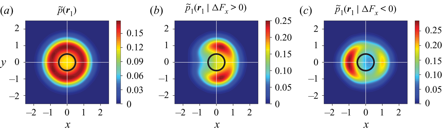
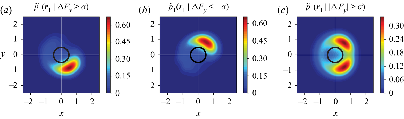
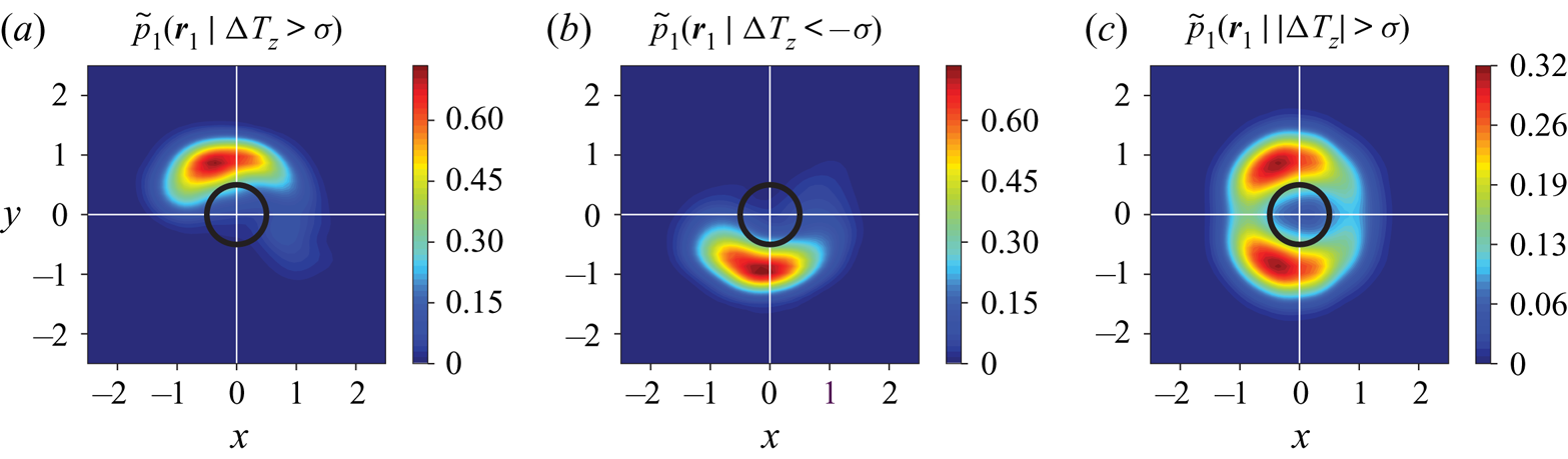
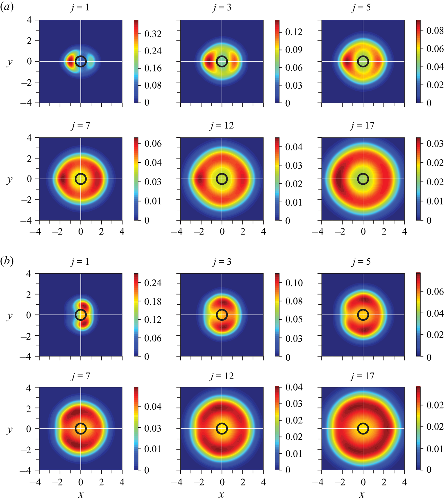
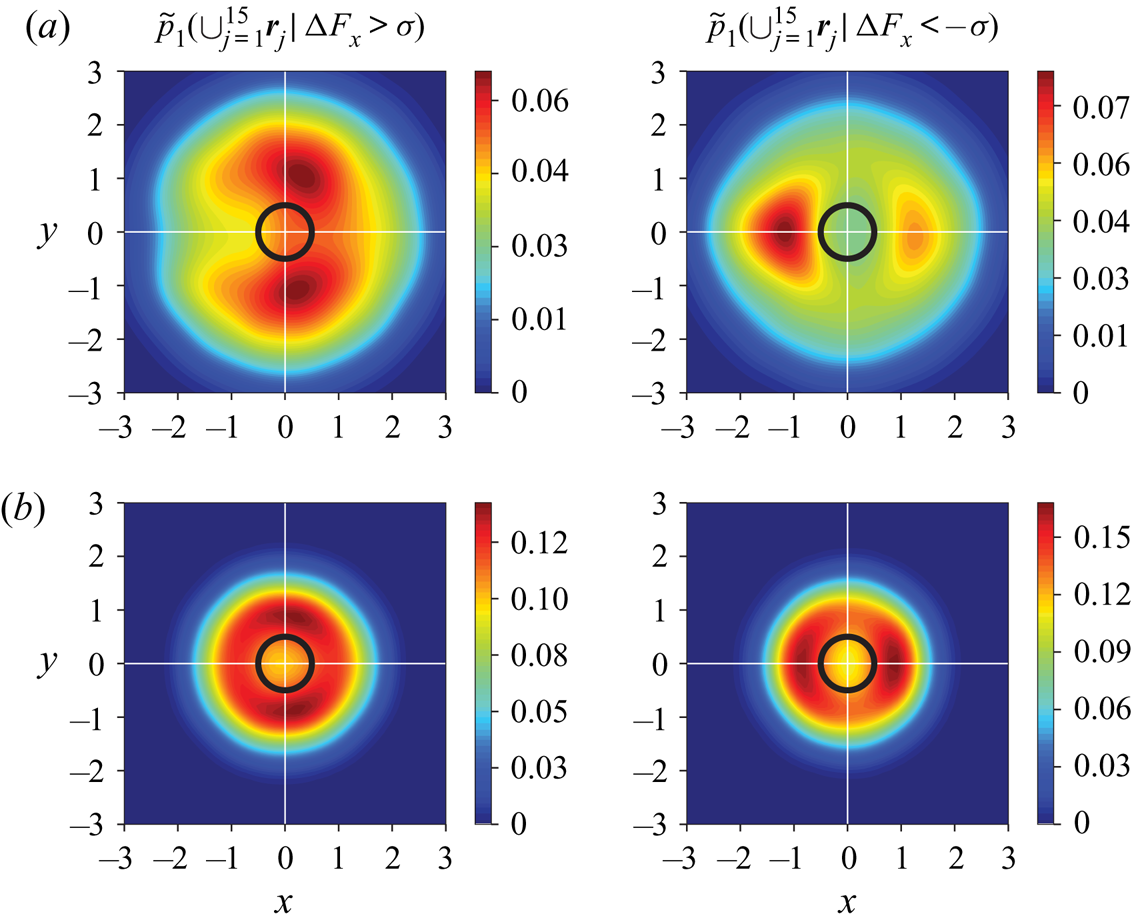
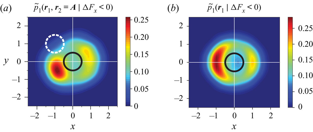
In this section, we scrutinise a few of the probability distribution maps obtained for different force/torque components and various neighbours. Before proceeding further, we first describe the necessary steps taken for generating the foregoing distributions. In order to construct the maps, those particles that satisfy the desired condition (e.g.  ${\rm \Delta} F_x < 0$ or
 $|{\rm \Delta} F_y| > \sigma$, with
 $\sigma$ being the standard deviation of the corresponding variable) are identified and filtered by looping over the entire array of spheres. In this filtered subset of the original data, the positions of the chosen neighbours are recorded. These positions constitute data points to which KDE functions in (3.19)–(3.21) are then fitted, thus giving
 $\tilde {p}_j \left (\boldsymbol {r}_j \: \vert \: \cdot \right )$. The generated PDFs are functions of the three spatial coordinates, which makes it impossible to visualise these functions directly. Inevitably, we resort to contour plots of the PDFs; however, three-dimensional contour surfaces are also neither efficient nor convenient to visualise. Consequently, we have opted for depicting their projections on two-dimensional planes. In doing so, the contour surfaces are entirely compressed onto an
 $x$–
 $y$ plane. This is why the reference particle will be shown as a blank circle in contrast to a solid disk, since the neighbouring spheres can happen to be located even at
 $(x,y) = (0,0)$ when
 $|z| \geq 0.5$.
In the case of streamwise force, all maps are in fact axisymmetric about the  $x$ axis; meaning that the choice of the plane on which the maps are shown does not make any difference, as long as it is parallel to the
 $x$ axis. As for the lateral forces, the maps are plane symmetric with respect to the same plane whose normal has the same direction as the force component (e.g.
 $\tilde {p} \left (\boldsymbol {r}_j \: \vert \: |{\rm \Delta} F_y| > \sigma \right )$ would be symmetric about the
 $y$ axis). For the hydrodynamic torques, the maps are also plane symmetric but with respect to the plane that contains the torque component. Owing to the symmetry about the streamwise direction, the probability distribution map for
 $|{\rm \Delta} F_y | > \sigma$ shown on the
 $x$–
 $y$ plane is essentially almost identical to that for
 $|{\rm \Delta} F_z | > \sigma$ on the
 $y$–
 $z$ plane. The same is also true for
 $|{\rm \Delta} T_z | > \sigma$ on
 $x$–
 $y$ and
 $|{\rm \Delta} T_y | > \sigma$ on
 $y$–
 $z$. Noting the existence of this similarity, only projections on the
 $x$–
 $y$ plane will be shown in this section. With an ideal densely populated dataset, the PDFs are expected to exhibit perfect symmetry. The limited number of samples in our dataset, however, causes some PDFs to show minor yet noticeable deviations from symmetry. This would be particularly evident in PDFs generated for farther neighbours due to the lower data density compared with closer neighbours. In what follows, statistical symmetry is hence enforced in all PDF depictions.
Examination of the probability maps in all cases remarkably reveals quite distinct, non-uniform and physically meaningful functional forms. Figure 4 shows the distribution of the first (i.e. closest) neighbour positions, conditioned on two different ranges of the streamwise force, while the blank circle in the middle of represents the reference particle which experiences the hydrodynamic force or torque. According to these probability maps, it is considerably more likely for a reference particle to experience higher than the mean drag force when the closest neighbour is located laterally, and slightly downstream of the particle. The right plot in figure 4 appears more intuitive: drag force diminishes if the reference particle is shielded by the closest neighbour directly in front of it, as expected. A somewhat less intuitive observation is that even if the neighbour happens to be immediately downstream of the reference particle, drag force would be lower than average, due to the suppression of the low-pressure region behind the reference particle. It is crucial to stress this point once more that these maps demonstrate the higher likelihood of coming across neighbours at particular regions depending on the condition imposed on force/torque fluctuation. This means that, for instance, even if the closest neighbour occurs to be located laterally, the drag force might be lower than average because the second neighbour happens to directly shield the reference particle. It signifies the fact that while accounting for the influence of one neighbour provides a great deal of valuable information about the fluctuations, effects of other neighbours are indispensable in explaining the force/torque fluctuation accurately.
(a) Unconditioned PDF of the first closest neighbour position and PDF of the first closest neighbour position when the reference particle experiences a (b) higher than average or (c) lower than average drag force. The PDFs are obtained for the case of  $Re = 40$ and
 $\phi = 0.1$.

Figures 5 and 6 show PDFs for the distribution of closest neighbours when conditions are imposed on the lateral force in the  $y$ direction and on the lateral torque in the
 $z$ direction, respectively. Note that for demonstration purposes, we have chosen more extreme conditions in figures 5 and 6, e.g.
 ${\rm \Delta} F_y > \sigma$ and
 ${\rm \Delta} F_y < -\sigma$, and
 ${\rm \Delta} T_z > \sigma$ and
 ${\rm \Delta} T_z < - \sigma$, respectively, in order to make the PDFs stand out more prominently. However, the MPP model ((3.25) and (3.26)) is always constructed with the original positive and negative conditioning (e.g.
 ${\rm \Delta} F_y > 0$ and
 ${\rm \Delta} F_y < 0$ for the lateral force in the
 $y$ direction). On the leftmost plot of figure 5, the reference particle is seen to experience a positive lateral force in the
 $y$ direction when the first neighbour is located within the region that lies mostly in the bottom right quadrant where
 $x > 0$ and
 $y < 0$, whereas a negative lateral force results when the first neighbour happens to be on the opposite side where
 $x, y > 0$ depicted in the middle plot. As pointed out by Prahl et al. (Reference Prahl, Hölzer, Arlov, Revstedt, Sommerfeld and Fuchs2007) for a staggered arrangement of only two spheres, a higher than normal pressure field develops in the gap between the two particles, which causes a repulsive force acting mainly on the upstream particle. Upon increasing the distance between the particles, the fluid can penetrate the gap more easily. The nozzle effect hence creates a low-pressure region in the gap which gives rise to an attraction force. The latter does not appear in figure 5 as the first neighbour is quite close to the reference particle, but regions corresponding to such a condition show up remarkably on the PDFs for the lateral force in case we consider more distant neighbours. The right most plot shows the PDFs conditioned with
 $|{\rm \Delta} F| > \sigma$, which is a combination of the foregoing plots with
 $\{ {\rm \Delta} F < -\sigma , {\rm \Delta} F > \sigma \}$. These are regions for which the reference particle experiences a non-zero lateral force in the
 $y$ direction.
The PDF of the first closest neighbour position when the reference particle experiences a (a) higher than  $\sigma$ or (b) lower than
 $\sigma$ lift, with
 $\sigma$ being the standard deviation of the data. (c) The PDF of the first closest neighbour position when the lift is either higher or lower than
 $\sigma$. The PDFs are obtained for the case of
 $Re = 40$ and
 $\phi = 0.1$.

The PDF of the first closest neighbour position when the reference particle experiences a (a) higher than  $\sigma$ and (b) lower than
 $\sigma$ lateral torque, with
 $\sigma$ being the standard deviation of the data. (c) The PDF of the first closest neighbour position when the lateral torque is either higher or lower than
 $\sigma$. The PDFs are obtained for the case of
 $Re = 40$ and
 $\phi = 0.1$.

In figure 6, we can see essentially the same kind of information as in figure 5. The most critical regions for the modification of the torque are located where the highest amount of vorticity is generated in the flow over a single sphere. As with the lateral force, the higher pressure in the gap decreases the fluid velocity and the resulting vorticity. The vorticity imbalance between the top and bottom regions of the reference particle brings about a net torque exerted on the particle. The interpretation of the PDFs emerging from our analysis is consistent with the observations made with a binary system of two spheres exhibiting the same dependency of the forces on relative positions of the spheres (Prahl et al. Reference Prahl, Hölzer, Arlov, Revstedt, Sommerfeld and Fuchs2007; Yoon & Yang Reference Yoon and Yang2007). Such modification of the forces and torques were also elucidated by Akiki et al. (Reference Akiki, Jackson and Balachandar2016). Our results imply that even when the system being modelled is a dense multi-particle system, the forces and torques acting on each particle still vary in the same manner on average, in response to the positioning of the closest neighbour. For instance, when a particle happens to experience less drag force, it is most probably shielded by an upstream neighbour (or supported by a neighbour immediately downstream with a comparatively less probability) as shown on the right plot in figure 4. Although this may not be always true, it is the most likely reason. Similar arguments apply in regards to all other conditional PDFs involving lateral forces and torques as well.
Interestingly, similar patterns are found for neighbours located further away. An example of the PDFs for farther neighbours is shown in figure 7. While the distributions are spread out and have become fainter for surrounding particles located farther away from the reference particle, regions with higher probability are discernible and turn out to be generally in accordance with those obtained for  $j=1$, i.e. the closest neighbour. The reason for the fact that the densities are smaller for
 $j > 1$ is twofold. First, farther particles are distributed over a larger volume around the reference particle. The second and more important reason is that the more distant particles are comparatively less likely to alter the force/torque fluctuations. The functional forms of
 $\tilde {p}$ in (3.16) has been kept distinct for each neighbour, meaning that
 $\tilde {p}_1$ is a different function compared with
 $\tilde {p}_2$, and they both are different from
 $\tilde {p_3}$ and so on. This is also reflected in the probability maps shown in figure 7. A possible simplification can be made by combining all functions
 $\tilde {p}_j$ into a single function
 $\tilde {p}$ that still contains the contribution of all included neighbours, except for not making distinction based on the ordering of the neighbours. In this manner, instead of filtering the locations of the
 $j$th neighbour, we filter the location of all the included neighbours (up to
 $j = M$) based on the desired condition. It is to be noted that we still retain the contribution of each neighbour to the net force/torque fluctuation by allowing separate terms for every included neighbour in (3.16). That is to say, we construct only one PDF, namely,
 $\tilde {p}$ using the entire neighbourhood, while each term
 $\tilde {p} \left (\boldsymbol {r}_j \: \vert \: \cdot \right )$ is assigned a separate unknown coefficient and influences the prediction of fluctuations differently. An example of such a combined PDF is shown for the streamwise force in figure 8(a) for
 $\phi = 0.1$. Comparing with figure 4, it is immediately obvious that the significant region around the reference particle has expanded due to the influence of more distant neighbours. Nevertheless, the general form of the maps that were obtained for
 $j = 1$ in figure 4 still prevails even when all the neighbours up to
 $j = M$ are included all at once. Another remarkable observation can be made from figure 8(b), where PDFs similar to those in figure 8(a) have been shown for the highest solid volume fraction of
 $\phi = 0.4$. The PDFs in figure 8(b) have gained fore-aft symmetry and are shrunk towards the reference particle, reminiscent of the force maps obtained with the data-driven model of Moore et al. (Reference Moore, Balachandar and Akiki2019) at
 $\phi = 0.45$.
The PDFs of various neighbour positions for (a)  ${\rm \Delta} F_x < - \sigma$, and (b)
 ${\rm \Delta} F_x > \sigma$, with
 $\sigma$ being the standard deviation of the data. Note that the numbering represented by
 $j$ is based on proximity to the reference particle, where
 $j=1$ shows the closest neighbour. The PDFs are obtained for
 $Re = 40$ and
 $\phi = 0.1$.

PDFs of positions of  $15$ closest neighbours for two different solid volume fractions. (a)
 $\textit {Re} = 40$ and
 $\phi = 0.1$, (b)
 $\textit {Re} = 40$ and
 $\phi = 0.4$.

4. Results and discussion
4.1. Practical aspects of implementation
4.1.1. Computational efficiency of KDE evaluations
Since the MPP model is to be used in EL simulations, at each time step it might be necessary to compute the forces and torques for several thousand, or perhaps millions of particles at once. The computational effort required for making predictions with the model is thus an important matter. The MPP model summarised in (3.18) consists of a handful of constant coefficients, multiplied by the same number of KDE-estimated PDFs. For  $m$ evaluations given
 $n$ sample points, evaluation of a KDE-estimated PDF by naive kernel summation in (3.19) (which we use for model computations in this work) requires a quadratic
 $O(mn)$ operations, which may be computationally prohibitive for the practical implementation of the MPP model. However, this issue can be circumvented to a great extent by using efficient approaches that have been proposed over the past years, including data binning with fast Fourier transform, fast sum updating, fast Gauss transform and the dual-tree method (Langrené & Warin Reference Langrené and Warin2019). The computational cost can be reduced from quadratic
 $O(mn)$ operations to linear
 $O(m + n)$ or
 $O( m \log m + n \log n )$, resulting in a vast improvement of computational efficiency by orders of magnitude compared with naive kernel summation.
Another possibility for speeding up probability density estimations is to approximate the density distributions with well-known functional forms such as polynomials or exponential functions. As KDE is a non-parametric estimation method, the dataset based on which predictions are made need to be stored in order to obtain KDE-estimated probability densities. Using simpler functional forms obviates the need for storing the dataset, albeit at the expense of potential loss of accuracy. Nevertheless, one needs to study the model degradation due to such approximations versus the gained speed up in computations, and decide how much of a trade-off is acceptable in a particular situation.
4.1.2. Model hyper-parameters
In our model, there are a few parameters that need to be given values before making predictions, and finely tuned to deliver optimal performance. These parameters are to be distinguished from the set of unknown constants of regression in (3.22), which can be deterministically found from the minimisation of sums of errors. Two important hyper-parameters involved in our model are the kernel bandwidth indicated by  $\boldsymbol{\mathsf{H}}$ in (3.20) and the number of included neighbours shown by
 $M$.
In its most general form the bandwidth is given by a symmetric, positive definite matrix when multidimensional data are concerned. The bandwidth  $\boldsymbol{\mathsf{H}}$ significantly influences the obtained KDEs through controlling the orientation and smoothing intensity of a kernel, equivalent to the standard deviation of a Gaussian distribution. A very narrow bandwidth results in a KDE with high variance, whereas an over-smoothed estimation is generated if the bandwidth is too wide. The former tends to capture specificities of a particular dataset resulting in an over-fitted model performing poorly on other datasets, while the latter fails to acquire the crucial patterns in the data, giving an overall weak prediction capability. Since in the present work, the neighbour positions are uniformly distributed in all three dimensions, choosing the same bandwidth for all directions is sensible. In this case, the bandwidth matrix is determined by a scalar
 $h$ such that
 $\boldsymbol{\mathsf{H}} = h \boldsymbol{\mathsf{J}}$ with
 $\boldsymbol{\mathsf{J}}$ being an all-ones matrix. A rule of thumb for estimating an optimal value for the bandwidth is given by Scott (Reference Scott1992) as
 $h = \sigma N^{-1/(D+4)}$, with
 $N$ as the number of samples and
 $D$ as the number of dimensions. In most of the cases in this work, we have used Scott's rule multiplied by a factor of 1–1.8. In most cases, a factor of
 $>$1 was necessary to avoid over-fitted results.
The other critical parameter to determine before attempting to make predictions is the number of neighbours to include in the modelling process. In low Reynolds number regimes, the force/torque fluctuations for each particle depend on a large number of surrounding particles (e.g. theoretically depending on each and every particle in the system for Stokes flow) due to the dominance of the elliptic nature of the governing equations at such regimes. In relatively inertial regimes, though, only a limited number of neighbouring particles influence the deviation of the hydrodynamic forces and torques acting on a particle from the average values. Akiki et al. (Reference Akiki, Jackson and Balachandar2017a) concluded that  $\approx$15–40 and
 $\approx$10 closest neighbours were required for optimal modelling of drag and lift, respectively, and that inclusion of more surrounding particles did not improve the quality of their physics-driven PIEP model in terms of the coefficient of determination
 $R^2$. For their data-driven PIEP model (Moore et al. Reference Moore, Balachandar and Akiki2019),
 $\approx$13 neighbours for drag and
 $\approx$15 neighbours for lift resulted in the best coefficient of determination. We have overall observed a similar trend for our MPP model concerning the number of neighbours to be included. A large number of neighbours have to be accounted for in lower
 $\textit {Re}$ for achieving maximum
 $R^2$, while this number decreases with the Reynolds number. Furthermore, we typically require fewer neighbours to include in order to model the lateral forces and torques compared with the streamwise force. Full details of the variation of the model quality with the number of neighbours will be given in the following sections.
Finally, another choice to be made is the type of kernel in (3.20). Different types of kernels such as parabolic (Epanechnikov), cosine, exponential and linear kernels can be alternatively used to give the weighted-average value at each point. As pointed out by Silverman (Reference Silverman1986), bandwidth selection is much more of a concern compared with the choice of the kernel, which can be legitimately based on the smoothness requirements or computational effort involved in making evaluations. In line with Silverman (Reference Silverman1986), our experimentation with different types of kernels indicates that the choice of the kernel type does not remarkably affect the performance of the model, given that optimal values of bandwidth are used.
4.1.3. Inclusion of average velocity
The channelling of the flow through the pores of a bed causes the fluid velocity experienced by the particles to fluctuate from particle to particle. This variance of undisturbed fluid velocity is partly dictated by the immediate neighbourhood of each particle, but not entirely. A bundle of a few particles might be collectively fully exposed to the fluid flow, while another group are mostly blocked by upstream neighbour groups. In the former case, the drag on a particle inside the bundle is significantly affected by its neighbours in the group, while in the latter case the particle would have experienced a relatively small or perhaps no drag, with little influence from its neighbours as the drag was not great to begin with. If we were able to include the effects of several neighbours around each particle instead of the approximation employed in (3.16), the channelling effect would theoretically be captured solely from the configuration of the neighbours. In the present work, this information can be directly supplied to the model by including a measure of the velocity seen by each particle. Since (3.18) is an approximation, linearly adding the average velocity seen by the particle may enhance the model. Therefore, (3.18) can be modified as follows:
 \begin{align} {\rm \Delta} F_{\textit{MPP}}(\boldsymbol{R}, \textit{Re}, \phi) &= \sum_{j=1}^M c_{\alpha, j} \, \tilde{p}_j \left(\boldsymbol{r}_j \: \vert \: {\rm \Delta} F < 0 \right)\nonumber\\ &\quad + \sum_{j=1}^M c_{\beta, j} \, \tilde{p}_j \left(\boldsymbol{r}_j \: \vert \: {\rm \Delta} F > 0 \right) + \sum_{d=1}^3 c_{\gamma,d} \overline{u}^v_d, \end{align}
where each  $c_{\gamma ,d}$ is an additional unknown coefficient, and
 $\overline {u}^v_d$ denotes an average velocity component of
 $\overline {\boldsymbol {u}}^v$ in
 $x$,
 $y$ or
 $z$ direction. The estimation of fluid velocity seen by a finite-size particle (i.e. undisturbed fluid velocity) within a multiparticle system is not straight-forward, resulting in several definitions in the literature (Bagchi & Balachandar Reference Bagchi and Balachandar2003; Kidanemariam et al. Reference Kidanemariam, Chan-Braun, Doychev and Uhlmann2013). Kidanemariam et al. (Reference Kidanemariam, Chan-Braun, Doychev and Uhlmann2013) suggest the average of fluid velocity taken on a spherical shell centred at the particle location as the characteristic fluid velocity; a definition also utilised by Uhlmann & Doychev (Reference Uhlmann and Doychev2014) in their analysis of settling suspensions of spheres. Here, we perform the phase-averaging in a spherical volume about the location of each particle to obtain the fluid velocity seen by the particle
 \begin{equation} \overline{\boldsymbol{u}}^v = \sum_{l=1}^{N_l} \Phi_l {\boldsymbol{u}_l} \left/\, \sum_{l=1}^{N_l} \Phi_l\right.\!, \end{equation}
where  $\Phi$ is the phase indicator function, which is utilised in order to avoid sampling velocity data inside the solid region, and
 $N_l$ the number of grid points falling within the spherical volume. The diameter of the averaging volume is chosen to be
 $4d$ for
 $\phi = \{ 0.1, 0.2 \}$ and
 $3d$ for
 $\phi =0.4$. The inclusion of the average velocity
 $\overline {\boldsymbol {u}}^v$ improves the predictions in all cases, reflected in the increasing of
 $R^2$ by up to
 $5\,\%$. This improvement is more pronounced for
 $\phi = 0.4$, resulting in an increase of up to
 $15\,\%$ in the coefficient of determination.
4.2. Model assessment
As a measure of performance, we will use the coefficient of determination defined as
 \begin{equation} R^2 = 1 - \frac{\displaystyle \sum_{i=1}^{N} \left( {\rm \Delta} F_{\textit{MPP}, i} - {\rm \Delta} F_{\textit{DNS}, i} \right)^{2}}{\displaystyle\sum_{i=1}^{N} \left( {\rm \Delta} F_{\textit{DNS}, i} - \langle {\rm \Delta} F_{\textit{DNS}, i} \rangle \right)^{2}}, \end{equation}
where  $N$ is the number of samples used for the computation of
 $R^2$. Also, we note that
 $\langle {\rm \Delta} F_{\textit{DNS}, i} \rangle = 0$ by definition. The coefficient of determination can be interpreted as the fraction of variations that are explained by the model. As such,
 $R^2 = 0$ implies that the particle-to-particle force/torque fluctuations are not captured at all and the model does not perform any better that giving a single average value for all particles. On the other hand,
 $R^2 = 1$ would indicate a perfect fit; i.e. fluctuations predicted by the model exactly match those obtained from PR-DNS.
With every data-driven model, it is necessary to ensure that the model has not only fitted the data in a satisfactory manner, but is also able to generalise its predictions to unseen data. Complex data-driven models in the realm of ML such as neural networks often have numerous unknown parameters which makes them prone to overfitting, particularly when dealing with small datasets. Put another way, an over-fitted model simply memorises the dataset thanks to its huge set of parameters, while it performs poorly when presented with unseen data. One strategy to prevent over-fitting and to assess the generalisation capability of a model is to split the dataset into a training set and a smaller validation set, so as to fit the model using the former and test its performance on the latter. This technique, commonly known as the hold-out method, works well if used with sufficiently large datasets. For datasets limited in size, such as data obtained from PR-DNS here, not only the validation set might not be sufficiently representative, the dataset is only partially utilised to train the model (Witten et al. Reference Witten, Frank, Hall and Pal2016). The  $K$-fold cross-validation is an assessment technique that randomly partitions the dataset into
 $K$ subsets or ‘folds’, so that one of these folds is held out for testing while the model is trained on the rest of
 $K - 1$ folds. This process is repeated with every partitioning such that the entire dataset has been used both for training and for validation. Any measure of error or accuracy and also the model's parameters may be averaged to give a more reliable estimation of the performance. To ensure the prediction reliability of the MPP model, we employ the
 $K$-fold cross validation with
 $K = 8$ where multiple rounds of cross-validation are performed using
 $K$ subsets of the data. All reported results are thus the averaged values over multiple rounds so that a reliable estimate of the model's predictive performance is achieved.
4.3. Performance of the MPP model
The results of the MPP model's predictions and comparison with our PR-DNS data are presented in terms of the coefficient of determination  $R^2$ in table 3. Note that we have deliberately avoided inclusion of data for
 ${\rm \Delta} F_z$ and
 ${\rm \Delta} T_y$, as the results obtained for these variables are equivalent to those for
 ${\rm \Delta} F_y$ and
 ${\rm \Delta} T_z$, respectively. The green and light green cells in table 3 refer to cases for which
 $R^2 \geq 0.7$ and
 $R^2 \geq 0.6$, respectively, and cells highlighted in red represents cases for which
 $R^2 \leq 0.5$. Overall, the MPP model exhibits a remarkable ability to correlate the observed force/torque deviations from the average values to the specific neighbourhood of each particle. Our proposed model is able to explain up to
 $84\,\%$,
 $78\,\%$ and
 $85\,\%$ of the drag, lift and torque variations, respectively, in the best cases with a mean coefficient of determination of
 $R^2 = 0.68$,
 $0.63$ and
 $0.67$ averaged over all cases. Except for three cases (shown in light red in table 3), at least
 $50\,\%$ of the particle-to-particle force/torque variations are captured by the model, while in most cases the coefficient of determination is seen to be greater than
 $60\,\%$. In figure 9 correlation scatter plots are shown for the stream-wise force or drag, the lateral force or lift and the lateral component of the torque. For each hydrodynamic load, we have selected three cases representing a range of Reynolds numbers and solid volume fractions in increasing order, in order to demonstrate cases where the model exhibits varying degrees of performance. The horizontal coordinate of each point on the plots shows the value of the force/torque deviation obtained from PR-DNS, whereas the vertical coordinate shows the value predicted by the present MPP model for the same sample in the dataset. The red bisector in figure 9 indicates a perfect fit, for which
 ${\rm \Delta} F_{\textit{MPP}} = {\rm \Delta} F_{\textit{DNS}}$ and
 $R^2 = 1$. Notably, the classical microstructure-ignorant drag correlations of the form
 $F = \langle F \rangle (\textit {Re}, \phi )$ in § 2.4 would all lie on a horizontal line given by
 ${\rm \Delta} F = 0$ in figure 9, since these correlations only give an average value for an entire ensemble of particles and are thus unable to explain any particle-to-particle variation of the drag. Clearly, the MPP model is not perfect in any of the cases, but the improvements over conventional correlations are substantial, reaching up to
 $R^2 = 0.84$,
 $0.77$ and
 $0.85$ for
 ${\rm \Delta} F_x$,
 ${\rm \Delta} F_y$ and
 ${\rm \Delta} T_z$ in best cases where
 $(\textit {Re}, \phi ) = (2, 0.1)$. As both
 $\textit {Re}$ and
 $\phi$ are increased from left to right in figure 9, the performance of the model suffers to some extent. Remarkably, however, the drag variation is still captured up to
 $61\,\%$ at the extreme case of
 $(\textit{Re}, \phi ) = (150, 0.4)$, while
 $R^2$ remains in the range of
 $0.66{-}0.71$ for all variables at
 $(\textit {Re}, \phi ) = (40, 0.2)$.
Regression plots for the drag, lift and lateral torque for various Reynolds numbers and solid volume fractions. The oblique red line in each plot shows an ideal fit.

Performance of the MPP model represented by the coefficient of determination  $R^2$ for cases considered in this work.

The approximation in (3.16) that  $\tilde {p} \left (\boldsymbol {R} \: \vert \: \cdot \right )$ (i.e. the PDF depending on locations of all included neighbours) may be estimated as a linear combination of
 $\tilde {p}_j \left (\boldsymbol {r}_j \: \vert \: \cdot \right )$ functions (i.e. marginal PDFs each depending on the location of only a single neighbour) imposes an important limit on how accurate the model can be. For instance, in case the joint distribution
 $\tilde {p}_{1,2} \left (\boldsymbol {r}_1, \boldsymbol {r}_2 \: \vert \: \cdot \right )$ is practical to obtain, the functional form of
 $\tilde {p}$ for the first neighbour would be different depending on where the second neighbour is located. In such a situation, the PDF for the drag in figure 4 would no longer be axisymmetric about the
 $x$ axis; it would take on different forms depending on where the second closest neighbour is located. An example of such a case is shown on the left-hand side of the PDF in figure 10. On the left plot, we have fixed the location of the second neighbour (shown as the grey circle) to stay within a small radius of
 $\boldsymbol {r}_2 = \boldsymbol {A} = (-1, 1, z)$ on
 $x$–
 $y$ plane, while the
 $z$ coordinate is left free. On the right, we have reiterated the right-hand side plot of figure 4, where the PDF is obtained by conditioning only the drag and observing the locations of the first neighbour. Obviously, the presence of the second neighbour has affected the probability distribution of the first neighbour's position which is indicated by pushing the upstream probability density peak downwards and shrinking it simultaneously. This alteration of the PDF is partially, but not merely, due to an exclusion of the space occupied by second neighbour, but also owing to the modification of the flow field induced by the particular positioning of the second neighbour. Notably, the first neighbour can still happen to be located immediately upstream of the reference particle. In short, the second neighbour influences how the first neighbour affects the reference particle. This type of interaction dubbed as ‘ternary effects’, and also higher-order interactions of this type are ingredients of the flow physics sacrificed in (3.16) in exchange for a functional form that is practical to estimate.
The PDF of the first closest neighbour position (a) having a second neighbour (drawn as a dashed white circle) deliberately fixed on  $x$–
 $y$ plane at
 $\boldsymbol {r}_2 = \boldsymbol {A} = (-1, 1, z)$, (b) PDF of the first closest neighbour position, same as in figure 4(c). The PDFs are obtained for
 $\textit {Re} = 40, \phi = 0.1$.

In Stokes flow and dilute conditions, binary interactions prevail and high-order interactions are negligible, and the net effect arising from different neighbours can be given as a linear superposition of the influence of each individual neighbour. As the Reynolds number increases, linear addition of effects can no longer account for ternary and higher-order interactions, thus diminishing the validity of the linear combination of effects employed in (3.16). Consider the relatively low solid volume fraction cases with  $\phi = 0.1$ in table 3. As the Reynolds number increases, the performance of the MPP model deteriorates as expected as a result of the superposition of each neighbour's influence in (3.16). The coefficient of determination
 $R^2$, however, remains almost constant for
 $\phi = 0.2$ and counter-intuitively improves for
 $\phi = 0.4$ when the Reynolds number increases. When
 $\phi = 0.4$, the average interparticle distance is considerably smaller than for
 $\phi = 0.1$ making the PDFs more flattened and uniform, thus reducing the variability of the extracted probability map. The increase of the Reynolds number renders the distribution more anisotropic to some extent (also reflected in the higher standard deviation of higher
 $\textit {Re}$ cases for
 $\phi = 0.4$ in table 2) which leads to an improved
 $R^2$.
In order to be able to practically implement the MPP model, we separated the influence of each neighbour on the force/torque fluctuations of a reference particle by marginalisation of the probability distribution in (3.16), and expressed the net deviation as the linear combination of all effects. Although this assumption resembles the pairwise interaction assumption of Akiki et al. (Reference Akiki, Jackson and Balachandar2017a) in their physics-driven PIEP model, it is nevertheless inherently different. The pairwise interaction approximation employed by Akiki et al. (Reference Akiki, Jackson and Balachandar2017a) is based on binary interaction maps where there is no incorporated notion of solid volume fraction. In (3.16), however, each functional  $\tilde {p}_j \left (\boldsymbol {r}_j \: \vert \: \cdot \right )$ is obtained for neighbour
 $j$ in the presence of all other neighbouring spheres. In other words,
 $\tilde {p}_j \left (\boldsymbol {r}_j \: \vert \: \cdot \right )$ appears as a binary interaction in which the effects of all other neighbours are averaged, but still statistically present. This implies that the functional form of each
 $\tilde {p}_j$ is in fact dependent on the solid volume fraction, which may explain the superior performance of the present MPP model (and the data-driven PIEP model, for that matter) in a higher particle concentrations compared with physics-driven PIEP model. For the purpose of comparison, with the MPP model
 $R^2 = 0.67$ and
 $0.61$ for drag in
 $(\textit {Re}, \phi ) = (40, 0.4)$ and
 $(\textit {Re}, \phi ) = (150, 0.4)$, respectively; whereas
 $R^2 = 0.12$ and
 $0.24$ in
 $(\textit {Re}, \phi ) = (21, 0.45)$ and
 $(\textit {Re}, \phi ) = (115, 0.45)$, respectively, with the physics-driven PIEP model. Although
 $\textit {Re}$ and
 $\phi$ are not exactly the same for the cases here and for those considered by Moore et al. (Reference Moore, Balachandar and Akiki2019), a general comparison of results shows that the performance of the MPP model is on par with the hybrid PIEP model which combines the physics-driven and data-driven approaches.
Lastly, it must be pointed out that the present MPP model only considers static arrays of spheres. In a general particle-laden flow situation, however, particles will be in motion and the dynamic evolution of the system will depend on the positions as well as the motion of the particles. With the current formulation, inclusion of the translational and rotational velocity and acceleration of each neighbour in the PDFs of (3.18) will increase their dimensionality, thus rendering them impractical to use in their present form. Future investigations (similar to what has been done by Esteghamatian et al. (Reference Esteghamatian, Bernard, Lance, Hammouti and Wachs2017, Reference Esteghamatian, Euzenat, Hammouti, Lance and Wachs2018) for conventional EL techniques) are needed to evaluate the MPP model's performance when implemented in EL simulations through comparisons with corresponding PR-DNS cases. Such an assessment would be greatly beneficial in quantifying the significance of the inclusion of translational and rotational velocity and acceleration of the neighbours, and also to identify situations where such contributions might be more or less important.
5. Summary and conclusion
Numerical simulations are indispensable tools in analysing particle-laden flows, as experimental investigation of this type of flow is both very costly if not entirely impractical, while the extent to which details of these complex flows are available to experimental measurements is also quite limited. Particle transport in microfluidic separation devices or in highly dense particulate flows and heat transfer properties of combustion fluidised beds are a few examples for which resorting to numerical tools is inevitable in order to obtain the details of the physical processes. Most particle-laden flows of practical interest host billions of particles and span a space orders of magnitude larger than the size of individual particles. Even with the exponential growth of computing power, resolving all relevant scales is not within reach in the foreseeable future. In a higher intermediate (i.e. meso) scale, the fluid governing equations are averaged and solved in sub-volumes each containing a few particles, treating the fluid in an Eulerian way while still tracking each individual particle in a Lagrangian manner. Consequently, the computational cost is substantially lowered at the expense of the need to supply closure models for fluid–solid momentum exchange. As field variables are not available at the particle level, hydrodynamic interaction forces and torques cannot be directly computed and should hence be appropriately modelled. In relatively dense particle-laden systems, the flow varies on the scale of the particle dimension due to the pseudo-turbulence created by the neighbours. Conventional point-particle models that are parameterised only in terms of the Reynolds number and average solid volume fraction fail to account for the effects of the complex undisturbed flow on the drag. Microstructure-induced lateral forces and torques, on the other hand, have been neglected entirely in such models by definition. Given the fact that the physical fidelity of EL simulations directly relies on the accuracy of the interphase coupling scheme, developing force/torque models capable of incorporating the influence of local neighbourhood of particles is crucial.
In the present work, we have attempted to develop a deterministic model based on probabilistic arguments for hydrodynamic forces and torques exerted on each individual particle within a random array of fixed spheres. Owing to the unique neighbourhood of each particle, the flow in its vicinity is modified in a distinct way, giving rise to significant force and torque variations. The principal idea exploited by our MPP model is that conditioning force or torque deviations to positive or negative ranges results in the emergence of particularly interesting, non-uniform distributions of neighbour locations. That is to say, if particles (i.e. samples) that experience particular ranges of force/torque fluctuations are filtered, and in turn the positions of their neighbours are examined, we will find that their surrounding particles are always spatially distributed in remarkably non-uniform manners consistent with our physical understanding of binary interactions between two spheres. For instance, a neighbour located immediately upstream shields a particle from the oncoming flow and eliminates the frontal high pressure region in a binary system. Analysis of the neighbours distribution when the drag force is lower than average clearly demonstrates that this is still true even in dense arrays of sphere, which signifies that invaluable information can be extracted from PR-DNS for the dependence of forces/torques on the local neighbourhood. If a particle experience a low drag force, it is highly likely that the particle is shielded by an upstream neighbour. The same argument holds for other force/torque-conditioned cases as well. It is critically important that while in a binary system these observations are certain events, for an array of particles the occurrence of such events is probabilistic in nature. Upon fixing the location of one neighbour (i.e.  $M = 1$), the configuration of all other neighbours is still free to randomly change. Therefore, for a given location of a neighbour, the force/torque fluctuation on the reference particle would be represented by a distribution, not a fixed value unlike in a binary system. This is why the notion of the expected value is invoked in order to provide an average value of the experienced force/torques for a given location of one neighbour. Two conceptual extremes are worth reiterating.
(a) All neighbours are free (
$M = 0$). In this case, the expected value for force/torque deviation is zero, as the distribution is centred on ${\rm \Delta} F = 0$.(b) All neighbours are fixed (
$M = N_p - 1$). The distribution of force/torque deviation becomes extremely narrow (Dirac's delta function) as all sources of fluctuation are held fixed. The expected value for force/torque deviation approaches ${\rm \Delta} F = {\rm \Delta} F_{\textit{DNS}}$.


We note that in a binary system,  $M = N_p - 1 = 1$, therefore
 ${\rm \Delta} F = {\rm \Delta} F_{\textit{DNS}}$. Theoretically then, this framework can have varying degrees of accuracy approaching that of PR-DNS; practically, however, obtaining probability distribution maps for
 $M > 1$ requires exponentially more samples to sufficiently cover the input space of the problem. We recognise the case
 $M = 1$ as representing first-order effects, while higher-order effects may be captured by fixing the positions of two or more neighbours simultaneously (i.e.
 $M \geq 2$, which translates into, for instance, obtaining
 $\tilde {p} \left (\boldsymbol {r}_1, \boldsymbol {r}_2 \: \vert \: \cdot \right )$ instead of
 $\tilde {p} \left (\boldsymbol {r}_1 \: \vert \: \cdot \right )$ only). In the present work, we have considered
 $M = 1$ as a first step of improvement over microstructure-ignorant classical correlations. In order to estimate forces and torques, we establish a framework to obtain the expected value of the force/torque deviations from the mean by taking advantage of the force/torque-conditioned probability distribution functions of neighbour locations. These distributions are approximated using KDEs which serve as basis functions for regression. The effect of each neighbour on the deviations is then linearly combined and the value of unknown coefficients is found through an ordinary least-squares regression method. With
 $M = 1$, adding more neighbours results in the linear addition of more terms, meaning that the functional form of the PDFs do not change. For
 $M = 2$, the PDFs themselves would change depending on where the second neighbour is located in addition to the firs neighbour, as alluded to in figure 10.
We have generated a dataset consisting of several cases at various Reynolds numbers and solid volume fractions relevant to dense particle-laden systems of interest. Following the aforementioned discussion, the model is not expected to be perfect when  $M = 1$. Nevertheless, the MPP model demonstrates remarkable performance by explaining up to 60 %–70 % of particle-to-particle force/torque variation in most cases, while for a few cases in the low
 $\textit {Re}$ and
 $\phi$ the percentage of explained variance in the data rises to up to
 $85\,\%$. We experimented with the model to examine the dependence of the model performance on the number of neighbours included in the superposition of effects. (Note that in the present work, the probability distribution functions are all generated by considering only one neighbour, i.e.
 $M = 1$. The number of included neighbours in figure 11 only determines how many of these PDFs are superposed to make a final prediction.) As shown in figure 11, we found out that inclusion of
 $\approx$20 neighbours is adequate for gaining optimal performance for the streamwise force. The jump in
 $R^2$ is quite steep for lateral forces and torques, as the inclusion of
 $\approx$5–10 neighbours are sufficient to achieve the maximum performance for most cases. Consequently, the MPP model requires two probability distribution functions for negative and positive contributions, and a few constant coefficients (
 $\approx$10–40) to predict a significant portion of variations in force/torque components for given
 $\textit {Re}$ and
 $\phi$. Computing the probability densities requires evaluation of the KDEs in (3.19), which in turn needs the dataset samples based on which the model is constructed. The samples needed for KDE estimation can be easily stored and utilised along with the constant coefficients to make predictions in an EL simulation.
Coefficient of determination  $R^2$ as a function of the number of included neighbours
 $M$ used for construction of the model.

According to the results obtained by our MPP model and also by the PIEP model (Akiki et al. Reference Akiki, Jackson and Balachandar2017a,Reference Akiki, Moore and Balachandarb; Moore et al. Reference Moore, Balachandar and Akiki2019), the performance experiences a significant enhancement by only considering the first-order effects, hinting an asymptotic behaviour with inclusion of higher effects. Even though  $M = N_p - 1$ is theoretically needed (in construction of PDFs) to reach the PR-DNS accuracy, we anticipate that even considering the second-order effects properly renders the performance levels satisfactorily high to obviate the need for making the model more complex, as the gain would probably not be significant for
 $M \geq 3$. On the one hand, accounting for the first-order effects of local microstructure on forces and torques can effectively predict the occurrence of phenomena such as wake attraction or DKT, which is deemed the dominant mechanism in preferential concentration and clustering of suspensions (Yin & Koch Reference Yin and Koch2007, Reference Yin and Koch2008; Uhlmann & Doychev Reference Uhlmann and Doychev2014; Zaidi et al. Reference Zaidi, Tsuji and Tanaka2014). On the other hand, we have previously shown that transverse particle velocity fluctuations and granular temperature are considerably underestimated by using conventional drag correlations in EL simulations (Esteghamatian et al. Reference Esteghamatian, Bernard, Lance, Hammouti and Wachs2017, Reference Esteghamatian, Euzenat, Hammouti, Lance and Wachs2018) due to the unavailability of microstructure-induced lateral forces. The MPP model can play a promising role in alleviating both challenges in current meso-scale simulation tools.
Acknowledgements
We greatly appreciate the financial support of the Natural Sciences and Engineering Research Council of Canada (NSERC) via their Discovery Grant Program. This research was enabled by support provided by Compute Canada (http://www.computecanada.ca) through Anthony Wachs's 2019 Resources for Research Groups allocation qpf-764-ab.
Declaration of interests
The authors report no conflict of interest.