3.1 The free-draining bead–rod model

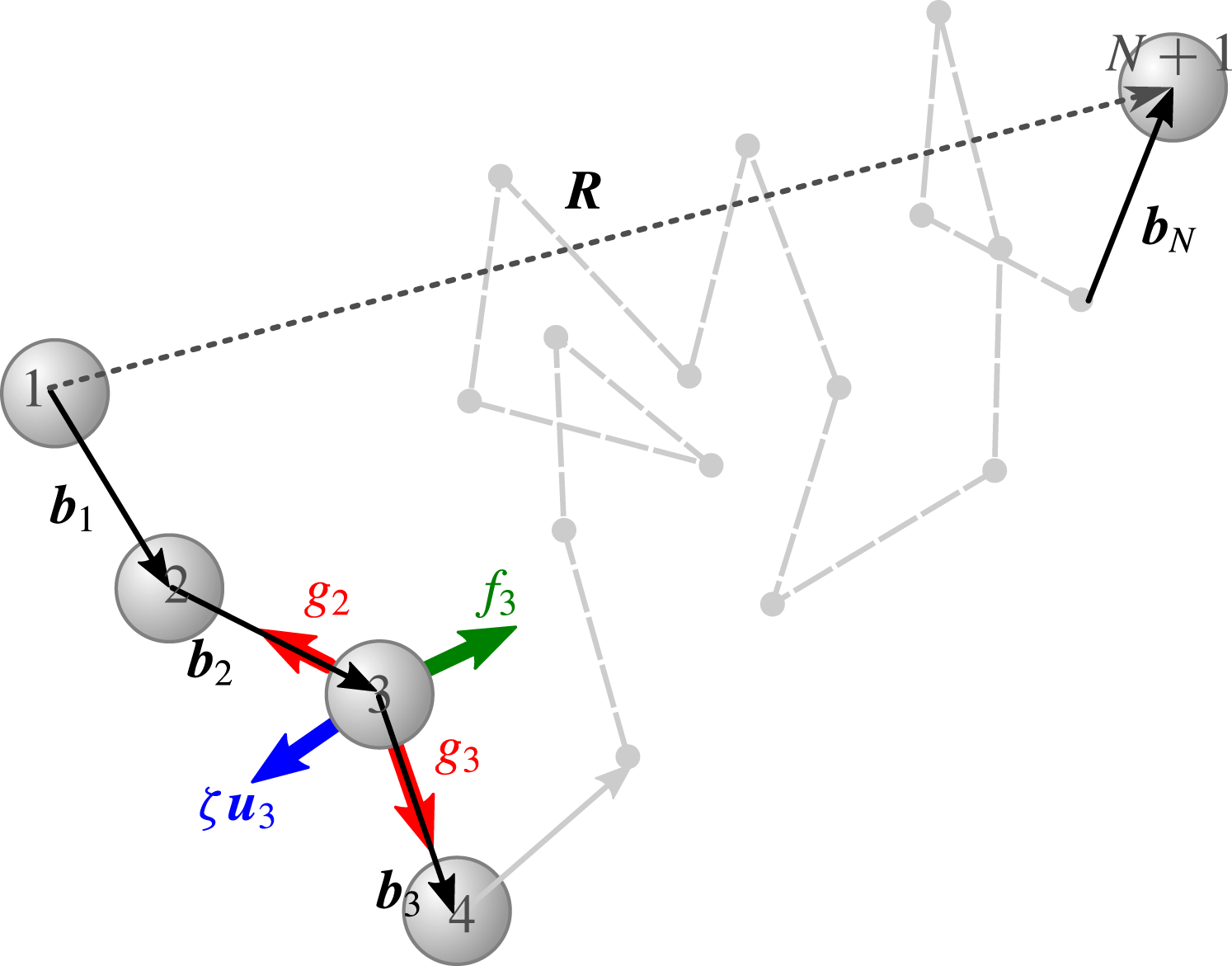
Following the work of Sim et al. (Reference Sim, Khomami and Sureshkumar2007), we employ the free-draining bead–rod model as our coarse-grained molecular approach. A complete description of this model may be found in Bird et al. (Reference Bird, Curtiss, Armstrong and Hassager1987), Liu (Reference Liu1989), Doyle, Shaqfeh & Gast (Reference Doyle, Shaqfeh and Gast1997), Sim et al. (Reference Sim, Khomami and Sureshkumar2007); we present here its main characteristics. The polymer chain is represented by a series of $N$ rigid rods connecting $N+1$ beads (see figure 2). The rods (vectors $\boldsymbol{b}_{1}$ , $\ldots$ , $\boldsymbol{b}_{N}$ ) are free to rotate but must keep a constant length $b$ , known as the Kuhn length. The sum of the rods gives the end-to-end vector, $\boldsymbol{R}$ . The equation of motion for the bead $i$ is given by:

(3.1) $$\begin{eqnarray}\displaystyle & \displaystyle \unicode[STIX]{x1D701}\boldsymbol{v}_{i}=\unicode[STIX]{x1D701}\boldsymbol{u}_{i}+g_{i}\boldsymbol{r}_{i}-g_{i-1}\boldsymbol{r}_{i-1}+\boldsymbol{f}_{i}, & \displaystyle\end{eqnarray}$$

where $\unicode[STIX]{x1D701}$ is the friction coefficient of the bead with the solvent, $\boldsymbol{u}_{i}$ is the unperturbed fluid velocity at the location of the bead (velocity field in absence of the chain), $g_{i}$ and $g_{i-1}$ are the internal tensions directed along the directions of the rods $\boldsymbol{r}_{i}=\boldsymbol{b}_{i}/b$ and $\boldsymbol{r}_{i-1}=\boldsymbol{b}_{i-1}/b$ (except at both ends of the chain where there is only one tension vector), and $\boldsymbol{f}_{i}$ a stochastic force modelling Brownian diffusion motion. The $\boldsymbol{f}_{i}$ are uncorrelated in space and time, of zero average and variance $2k_{B}T\unicode[STIX]{x1D701}$ for each space coordinate, $k_{B}T$ being the thermal energy. The evolution equation for each rod is then:

(3.2) $$\begin{eqnarray}\displaystyle & \displaystyle {\displaystyle \frac{\text{d}\boldsymbol{b}_{i}}{\text{d}t}}=\boldsymbol{v}_{i+1}-\boldsymbol{v}_{i}. & \displaystyle\end{eqnarray}$$

Integrating with an explicit Euler scheme over a time step $\unicode[STIX]{x1D6FF}t$ while enforcing the rod length to remain constant leads to the following system of equations for the internal tensions:

(3.3) $$\begin{eqnarray}\displaystyle & \displaystyle -g_{i+1}\boldsymbol{r}_{i}\boldsymbol{\cdot }\boldsymbol{r}_{i+1}+2g_{i}-g_{i-1}\boldsymbol{r}_{i}\boldsymbol{\cdot }\boldsymbol{r}_{i-1}=\unicode[STIX]{x1D701}b\,\boldsymbol{r}_{i}\boldsymbol{\cdot }\unicode[STIX]{x1D646}\boldsymbol{\cdot }\boldsymbol{r}_{i}+\boldsymbol{r}_{i}\boldsymbol{\cdot }(\boldsymbol{w}_{i+1}-\boldsymbol{w}_{i})+{\displaystyle \frac{\unicode[STIX]{x1D701}\unicode[STIX]{x1D6FF}t}{2b}}(\boldsymbol{v}_{i+1}-\boldsymbol{v}_{i})^{2}, & \displaystyle \nonumber\\ \displaystyle & & \displaystyle\end{eqnarray}$$

with $\unicode[STIX]{x1D646}=\unicode[STIX]{x1D735}\boldsymbol{u}^{\text{T}}$ is the transpose of the fluid velocity gradient and $\boldsymbol{w}_{i}$ are random vectors of mean zero and variance $2k_{B}T\unicode[STIX]{x1D701}/\unicode[STIX]{x1D6FF}t$ . The last term is nonlinear and is iteratively solved by a fixed point method.

Figure 2.

Bead–rod model for a polymer chain.

Equation (3.3) can be made dimensionless by dividing forces by $k_{B}T/b$ , lengths by $b$ and time by $\unicode[STIX]{x1D701}b^{2}/(k_{B}T)$ :

(3.4) $$\begin{eqnarray}\displaystyle & \displaystyle -g_{i+1}^{+}\boldsymbol{r}_{i}\boldsymbol{\cdot }\boldsymbol{r}_{i+1}+2g_{i}^{+}-g_{i-1}^{+}\boldsymbol{r}_{i}\boldsymbol{\cdot }\boldsymbol{r}_{i-1}=Pe\;\boldsymbol{r}_{i}\boldsymbol{\cdot }\unicode[STIX]{x1D646}\boldsymbol{\cdot }\boldsymbol{r}_{i}+\boldsymbol{r}_{i}\boldsymbol{\cdot }(\boldsymbol{w}_{i+1}-\boldsymbol{w}_{i})+{\displaystyle \frac{\unicode[STIX]{x1D6FF}t^{+}}{2}}(\boldsymbol{v}_{i+1}^{+}-\boldsymbol{v}_{i}^{+})^{2}, & \displaystyle \nonumber\\ \displaystyle & & \displaystyle\end{eqnarray}$$

with $^{+}$ indicating normalised quantities, and $Pe$ the Péclet number defined by:

(3.5) $$\begin{eqnarray}\displaystyle & \displaystyle Pe={\displaystyle \frac{\unicode[STIX]{x1D701}b^{2}\dot{\unicode[STIX]{x1D700}}}{k_{B}T}}, & \displaystyle\end{eqnarray}$$

where $\dot{\unicode[STIX]{x1D700}}$ is the characteristic extensional strain rate, such that $\unicode[STIX]{x1D646}=\dot{\unicode[STIX]{x1D700}}\unicode[STIX]{x1D646}^{+}$ . The Péclet number quantifies, at the scale of a single rod, the competition between the shuffling Brownian motion and the macroscopic fluid drive.

The Weissenberg number, $Wi$ , is another desirable characteristic variable needed to describe the dynamics of polymers in solution. It is defined by the product of the strain rate $\dot{\unicode[STIX]{x1D700}}$ times the longest relaxation time of the polymer. Using extensive simulations, Doyle et al. (Reference Doyle, Shaqfeh and Gast1997) proposed the scaling relation for the free-draining bead–rod model:

(3.6) $$\begin{eqnarray}\displaystyle & \displaystyle Wi=0.0142\,N^{2}\,Pe. & \displaystyle\end{eqnarray}$$

We note that the coefficient $0.0142$ is close to $1/(6\unicode[STIX]{x03C0}^{2})\approx 0.0169$ from the Rouse model.

A final remark has to be made about the free-draining nature of the model. Internal hydrodynamic interactions (HI) and excluded volume effects (EV) are known to have a significant impact on the dynamics of polymers in solution (Teraoka Reference Teraoka2002). Integrating these effects in simulations greatly increases the algorithm complexity and computational time. As a result, HI and EV have long been confined to the simulations of chains with very limited number of rods. Although notable improvements have been made in this field over the past few years (Banchio & Brady Reference Banchio and Brady2003; Geyer & Winter Reference Geyer and Winter2009; Schmidt, Cifre & García de la Torre Reference Schmidt, Cifre and García de la Torre2011; Saadat & Khomami Reference Saadat and Khomami2015; Moghani & Khomami Reference Moghani and Khomami2017), we decided not to incorporate HI and EV in our simulations for several reasons. First, the flexible and high molecular weight polymers of interest in this paper require large numbers of rods (over 1000), which still makes HI and EV computationally prohibitive. Second, previous simulations of the scission of moderate length chains have shown that the rupture dynamics do not depend strongly on the existence of HI and EV (López Cascales & García de la Torre Reference López Cascales and García de la Torre1991; Knudsen et al. Reference Knudsen, López Martinez and García de la Torre1996b ; Sim et al. Reference Sim, Khomami and Sureshkumar2007). This is due to the fact that the HI and EV coupling is weak near the fully stretched configuration, and in cases of practical importance, the chains are indeed mostly unravelled by the extensional flow before being broken.

3.2 Adaptive time stepping and rod coarse-graining

Even without modelling HI and EV effects, the simulation of bead–rod chains above $10^{4}$ rods over a few milliseconds of physical time requires substantial computing resources. It can be possible to study a single molecule but this approach quickly becomes unreasonable for a population of a few hundred. Two modifications have thus been made to the standard bead–rod algorithm in order to enhance its throughput.

First, we implemented an adaptive time stepping approach. The simulation of each chain starts with a normalised time step of $\unicode[STIX]{x1D6FF}t^{+}=10^{-3}$ , which is sufficiently fine for unravelled chain motion. However, as the chain catches more of the flow gradient, the time step has to be reduced, otherwise the iterative solver of (3.3) does not necessarily converge. This is done automatically by recursively halving the time step until convergence is reached. In this manner, the finer time dynamics are computed only when required.

The second modification is based on the consideration that the tension in a straight segment is essentially a parabola (Sim et al. Reference Sim, Khomami and Sureshkumar2007) and so can be described by a relatively small subset of rods. We performed this approximation by a coarse-graining of the chain at locations where the internal tension greatly exceeds the Brownian force, here: $g_{i}^{+}>100$ . Contiguous rods meeting this criterion are merged and the friction coefficients ( $\unicode[STIX]{x1D701}$ ) of remaining beads are increased accordingly. Typical speed-up factors of 20–140 can be achieved by allowing six recursive levels of rod merging.

3.3 Chain scission hypothesis

In the bead–rod model, we assume that a chain breaks if there is a rod where the internal tension reaches the value, $g_{c}$ , reflecting the breaking of a backbone bond. Typically reported values for a C–C single bond span from 2.6 nN to 13.4 nN, whether it is calculated from experiments or ab initio simulations, and possibly depend, though weakly, on the force loading rate (Odell & Keller Reference Odell and Keller1986; Grandbois et al. Reference Grandbois, Beyer, Rief, Clausen-Schaumann and Gaub1999; Beyer Reference Beyer2000; Stauch & Dreuw Reference Stauch and Dreuw2016). As explained in detail by Sim et al. (Reference Sim, Khomami and Sureshkumar2007), because of the discrete random forces $\boldsymbol{w}^{+}$ , solving (3.4) gives normalised tensions that fluctuate with variance scaling as $O(N/\unicode[STIX]{x1D6FF}t^{+})$ . If we want to set a threshold criterion for the internal tension, it is necessary to filter any unphysical fluctuations. Several methods have been proposed, requiring additional hypotheses or substantial postprocessing (Schieber & Obasanjo Reference Schieber and Obasanjo2005; Sim et al. Reference Sim, Khomami and Sureshkumar2007). Here, we choose a simpler approach. We do not remove completely the time-step dependent fluctuations, but keep them within the typical error margin of $g_{c}$ . To achieve this, the value of the tension is time-averaged over $p$ time steps. It follows that the variance of fluctuations is reduced to $O(N/(p\unicode[STIX]{x1D6FF}t^{+}))$ . We will see that the normalised rupture force, $g_{c}^{+}$ , is of the order of $10^{3}$ , over which we can assume a 10 % relative error. Therefore, by choosing $p>10^{-4}N/\unicode[STIX]{x1D6FF}t^{+}$ , we arrive at a reasonably smoothed estimate for the internal tension. On the other hand, $p$ should be kept as low as possible in order to keep track of the transient dynamics.

3.4 Setting dimensions of the bead–rod model

Two parameters are essential for setting the dimensions of the bead–rod model. First, the Kuhn length is assessed from tabulated data (Brandrup, Immergut & Grulke Reference Brandrup, Immergut and Grulke1999):

(3.7) $$\begin{eqnarray}\displaystyle & \displaystyle b={\displaystyle \frac{C_{\infty }\ell }{0.84}}, & \displaystyle\end{eqnarray}$$

where $C_{\infty }$ is a rigidity constant and $\ell$ the mean length of a backbone bond. It is then possible to know the number of rods required to represent a given molecular weight,  $M$ :

(3.8) $$\begin{eqnarray}\displaystyle & \displaystyle N={\displaystyle \frac{M}{M_{b}}}, & \displaystyle\end{eqnarray}$$

where $M_{b}$ is the molecular weight of a single rod, given by

(3.9) $$\begin{eqnarray}\displaystyle & \displaystyle M_{b}={\displaystyle \frac{M_{0}C_{\infty }}{0.84^{2}i}}, & \displaystyle\end{eqnarray}$$

with $M_{0}$ the monomer molecular weight and $i$ the number of backbone bonds per monomer. The second important physical parameter is the friction coefficient of the beads. It is usually assessed so that the longest relaxation time of the chain matches the Zimm relaxation time of the polymer, $\unicode[STIX]{x1D70F}_{Z}$ (Doyle et al. Reference Doyle, Shaqfeh and Gast1997). According to (3.6):

(3.10) $$\begin{eqnarray}\displaystyle & \displaystyle \unicode[STIX]{x1D701}={\displaystyle \frac{k_{B}T\unicode[STIX]{x1D70F}_{Z}}{0.0142N^{2}b^{2}}}. & \displaystyle\end{eqnarray}$$

The Zimm time can be computed from:

(3.11) $$\begin{eqnarray}\displaystyle & \displaystyle \unicode[STIX]{x1D70F}_{Z}={\displaystyle \frac{[\unicode[STIX]{x1D702}]\unicode[STIX]{x1D702}_{s}M}{RT}}, & \displaystyle\end{eqnarray}$$

with $[\unicode[STIX]{x1D702}]$ the intrinsic viscosity, $\unicode[STIX]{x1D702}_{s}$ the viscosity of the solvent, and $R$ the gas constant. In turn, $[\unicode[STIX]{x1D702}]$ , which is a function of the molecular weight and solvent properties, is tabulated through the use of the Mark–Houwink–Sakurada law:

(3.12) $$\begin{eqnarray}\displaystyle & \displaystyle [\unicode[STIX]{x1D702}]=KM^{a}, & \displaystyle\end{eqnarray}$$

where $K$ and $a$ are constants depending on the solvent and on temperature.

The Zimm time is relevant to the polymer dynamics in its coil state. We see from (3.11) and (3.12) that the scaling with the molecular weight is $M^{a+1}$ , quite different from the free-draining $M^{2}$ (3.6). Yet, near full extension, the hydrodynamic shielding of the chain vanishes, and a correct friction coefficient has to be chosen. We can assess this coefficient by taking its value for a single Kuhn step:

(3.13) $$\begin{eqnarray}\displaystyle & \displaystyle \unicode[STIX]{x1D701}_{b}={\displaystyle \frac{\unicode[STIX]{x1D702}_{s}KM_{b}^{a+1}}{0.0142{\mathcal{N}}_{A}b^{2}}}, & \displaystyle\end{eqnarray}$$

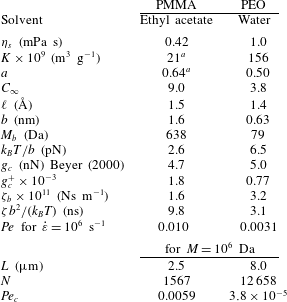
with ${\mathcal{N}}_{A}$ the Avogadro number. Table 1 summarises experimentally determined parameters for two polymer solutions: poly(methyl methacrylate) (PMMA) in ethyl acetate, and PEO in water. Molecular constants are taken from Brandrup et al. (Reference Brandrup, Immergut and Grulke1999).

Table 1.

Dimensioning parameters for the bead–rod model (room temperature).

a From in-house viscometric measurement.

3.5 Tension in a fully stretched chain

The internal tension in a fully stretched chain will be the starting point of our macroscopic formulation. By fully stretched, we mean that the rods are perfectly aligned with each other. If, in addition, the chain is stretched in a uniaxial extensional flow and aligned with the strain axis, it is known that the internal tension has a parabolic shape with a maximum at the centre of the molecule, given by (Sim et al. Reference Sim, Khomami and Sureshkumar2007):

(3.14) $$\begin{eqnarray}\displaystyle & \displaystyle g_{\max }={\displaystyle \frac{\unicode[STIX]{x1D701}\dot{\unicode[STIX]{x1D700}}L^{2}}{8b}}, & \displaystyle\end{eqnarray}$$

with $L$ the contour length of the molecule. This expression can be generalised to an arbitrary flow field where the chain is still fully stretched but not necessarily aligned with the elongation:

(3.15) $$\begin{eqnarray}\displaystyle & \displaystyle g_{\max }={\displaystyle \frac{\unicode[STIX]{x1D701}\unicode[STIX]{x1D735}\boldsymbol{u}\mathbf{:}\boldsymbol{R}\boldsymbol{R}}{8b}}. & \displaystyle\end{eqnarray}$$

This expression is ensemble-averaged to get:

(3.16) $$\begin{eqnarray}\displaystyle & \displaystyle \langle g_{\max }\rangle ={\displaystyle \frac{\unicode[STIX]{x1D701}\unicode[STIX]{x1D735}\boldsymbol{u}\mathbf{:}\unicode[STIX]{x1D63C}}{8b}}, & \displaystyle\end{eqnarray}$$

where we have introduced the conformation tensor $\unicode[STIX]{x1D63C}$ defined in § 2. Equation (3.16) is an expression of the average maximum internal tension as a function of macroscopic quantities. Albeit derived for a steady state elongation, we will see in the following that it provides a good approximation in transient and arbitrary flows.

3.6 Reaction rate

López Cascales & García de la Torre (Reference López Cascales and García de la Torre1992) studied the chemical kinetics of chain fracture under a sudden elongational flow. They employed two bead–spring models, each with a specific elastic function and maximum stretching energy for the springs. They found that the reaction kinetics can be described by two regimes: a first period of time when the chains align with the flow and start unravelling; then a second step when the chains break following a first-order reaction rate. They analysed the scaling of the reaction constant with the strain rate and the number of beads.

In practical flows however, the extensional rate varies either when the flow is transient, or when the molecules travel through regions of different flow gradients. For example, let us consider a population of random coils subject to an increasing Péclet number (increasing strain rate). According to (3.14), we can define a critical Péclet for the onset of chain rupture:

(3.17) $$\begin{eqnarray}\displaystyle & \displaystyle Pe_{c}={\displaystyle \frac{8g_{c}^{+}}{N^{2}}}. & \displaystyle\end{eqnarray}$$

For $Wi>1/2$ , the chains unravel, but do not break as long as $Pe<Pe_{c}$ . If they stay in this situation during at least a few $Pe^{-1}$ (in normalised time units), they unravel completely and the population is composed of homogeneous stretched chains. The tension in each chain then differs from $\langle g_{\max }\rangle$ only by thermal fluctuations. Then, if at this stage, $Pe\geqslant Pe_{c}$ , all the chains break simultaneously regarding the macroscopic time scale. On the other hand, if $Pe$ becomes greater than $Pe_{c}$ in less than $Pe^{-1}$ (which is the case for the sudden elongation in López Cascales & García de la Torre (Reference López Cascales and García de la Torre1992) and contraction flows in general), only the chains that have significant unravelled portions break. The rate at which the population of intact chains decreases depends on the unravelling dynamics of individual molecules.

Figure 3.

Bead–rod model simulation of the evolution of the relative concentration of intact chains subject to a sudden extensional flow of various strength. (a) PMMA ( $N=1567$ , $Pe_{c}=5.9\times 10^{-3}$ ), (b) PEO ( $N=12\,658$ , $Pe_{c}=3.8\times 10^{-5}$ ).

For a sudden elongation, we reproduced the numerical experiment of López Cascales & García de la Torre (Reference López Cascales and García de la Torre1992) but with the free-draining bead–rod model presented above. We use the parameters of table 1 for the PMMA 1 MDa and the PEO 1 MDa solutions. Results for various strain rates are reported in figure 3. For every strain rate, 256 molecules with random initial configurations are simulated and chain scission events recorded. The normalised concentration $c^{+}$ of initial chains is plotted against the total strain $Pe\,t^{+}$ . At long times (equivalently at high strain), an exponential decrease in $c^{+}$ is found, suggesting again a first-order scission rate. The rate constant is $Pe/2$ if the critical tension is close to the tension in the fully stretched chain, in other words, $Pe\sim Pe_{c}$ (chains unravel first, then break), and higher if $Pe\gg Pe_{c}$ . More specifically, our bead–rod simulations show that, when $Pe$ is close to $Pe_{c}$ , the concentration $c^{+}$ is fairly represented by the functional form:

(3.18) $$\begin{eqnarray}\displaystyle & \displaystyle c^{+}=(1-\unicode[STIX]{x1D706}^{2})^{Pe/Pe_{c}}, & \displaystyle\end{eqnarray}$$

where $\unicode[STIX]{x1D706}=\text{tr}(\unicode[STIX]{x1D63C})/L^{2}$ is the normalised extension of the chains. A convenient way of estimating $Pe$ through $\dot{\unicode[STIX]{x1D700}}$ in arbitrary flow is $\dot{\unicode[STIX]{x1D700}}\approx \unicode[STIX]{x1D735}\boldsymbol{u}\boldsymbol{ : }\unicode[STIX]{x1D63C}/\text{tr}(\unicode[STIX]{x1D63C})$ . The ratio $Pe/Pe_{c}$ can then also be put in terms of the internal tension, according to (3.16) and (3.17): $Pe/Pe_{c}\approx \langle g^{+}\rangle /(\unicode[STIX]{x1D706}g_{c}^{+})$ . The first-order kinetic coefficient, $k$ , defined by $k=-(\text{d}/\text{d}t)\ln c^{+}$ is then:

(3.19) $$\begin{eqnarray}\displaystyle & \displaystyle k=-{\displaystyle \frac{\text{d}}{\text{d}t}}\left[{\displaystyle \frac{\langle g^{+}\rangle }{\unicode[STIX]{x1D706}g_{c}^{+}}}\ln (1-\unicode[STIX]{x1D706}^{2})\right]. & \displaystyle\end{eqnarray}$$

Equation (3.19) gives a general model for chain scission, complemented with the following assumptions:

1. (i) No recombination of chains: $k\geqslant 0$ . In particular, $k=0$ for relaxing chains with $\text{d}\langle g^{+}\rangle /\text{d}t<0$ .

2. (ii) No scission occurs below the threshold Péclet number: $k=0$ for $Pe<Pe_{c}$ .

Note that we restrict the model to the scission of the initial chains only. If strain rates are sufficiently high, scission products might break in turn, as demonstrated by experiments and simulations (Odell & Keller Reference Odell and Keller1986; Sim et al. Reference Sim, Khomami and Sureshkumar2007).

3.7 CFD model

In the previous subsections, we obtained closed forms of the ensemble-average peak tension in chains and of the scission kinetic rate as functions of the conformation tensor. What remains to be chosen is then the constitutive equation to solve $\unicode[STIX]{x1D63C}$ at the macroscopic scale. Here, we employ an upper-convected model adapted from Hinch (Reference Hinch1994):

(3.20) $$\begin{eqnarray}\displaystyle & \displaystyle \overset{\triangledown }{\unicode[STIX]{x1D63C}}=-\max \!\left[0,\left({\displaystyle \frac{7}{2}}-{\displaystyle \frac{3}{2}}\unicode[STIX]{x1D706}\right)\unicode[STIX]{x1D735}\boldsymbol{u}\boldsymbol{ : }{\displaystyle \frac{\unicode[STIX]{x1D63C}}{L^{2}}}\right]\unicode[STIX]{x1D63C}-{\displaystyle \frac{\unicode[STIX]{x1D63C}-{\displaystyle \frac{R_{0}^{2}}{3}}\unicode[STIX]{x1D644}}{\unicode[STIX]{x1D70F}}}, & \displaystyle\end{eqnarray}$$

where $\overset{\triangledown }{\unicode[STIX]{x1D63C}}=(\text{d}/\text{d}t)\unicode[STIX]{x1D63C}-\unicode[STIX]{x1D735}\boldsymbol{u}^{\text{T}}\unicode[STIX]{x1D63C}-\unicode[STIX]{x1D63C}\unicode[STIX]{x1D735}\boldsymbol{u}$ is the upper-convected derivative of $\unicode[STIX]{x1D63C}$ , $R_{0}$ is the ensemble-averaged end-to-end distance of the unperturbed chains, $\unicode[STIX]{x1D644}$ is the identity tensor and $\unicode[STIX]{x1D70F}$ is a relaxation time. The first term of the right-hand side accounts for both the unravelling dynamics and finite extensibility of the chains. Although this term has the form of an internal viscosity, it is not due to any frictional process, but rather to the complex topological evolution of unfolding kinks (Hinch Reference Hinch1994). When the inner product $\unicode[STIX]{x1D735}\boldsymbol{u}\boldsymbol{ : }\unicode[STIX]{x1D63C}$ is negative, the chains are contracting, and this effective internal viscosity has to be set to zero. From our uniaxial extension simulations of bead–rod chains, we found that the $(7/2-3/2\unicode[STIX]{x1D706})$ factor is necessary to ensure that the conformation converges exponentially towards fully stretched chains at the correct rate of $\dot{\unicode[STIX]{x1D700}}/2$ . The second term of the right-hand side is an exponential relaxation in the absence of flow gradient. The relevance of (3.20) can be tested by plotting $\unicode[STIX]{x1D706}$ as a function of time during the sudden elongation simulations of the previous subsection. Results are shown in figure 4, where another common constitutive equation, the FENE-P model (finitely extensible nonlinear elastic with Peterlin closure, Bird & Wiest Reference Bird and Wiest1995) is also plotted. In particular, we see that the internal viscosity term is necessary to capture the slowdown of unravelling towards the steady state.

Figure 4.

Unravelling dynamics of PMMA chains ( $N=1567$ ) during a sudden elongation.

Effects such as hydrodynamic interactions, concentration or multimode relaxation are neglected here, but could be incorporated in more complex or empirical models (Lielens et al. Reference Lielens, Keunings and Legat1999; Ilg et al. Reference Ilg, Mavrantzas, Öttinger, Gujrati and Leonov2010). In addition, we assume very dilute concentrations, so that the viscous stress tensor is not affected by the presence of polymers. This is justified as an initial approach by the fact that the scission rate depends on local flow gradients, regardless of whether the shape of the flow was influenced by non-Newtonian effects or not. By doing so, the velocity field of the fluid is not coupled with the conformation tensor and can be solved by a standard method.

The scission model was implemented using the C++ library OpenFOAM (Weller et al. Reference Weller, Tabor, Jasak and Fureby1998; Favero et al. Reference Favero, Secchi, Cardozo and Jasak2010). The CFD solver can be summarised as follows. For each time step:

1. (i) The velocity $\boldsymbol{u}$ and pressure fields are solved using the PISO algorithm (OpenFOAM standard solver);

2. (ii) $\unicode[STIX]{x1D63C}$ is solved (3.20);

3. (iii) $\langle g\rangle$ and $k$ are updated (3.16) and (3.19);

4. (iv) $c$ is solved (convected scalar with a first-order mass sink).

In the next section, we present simulation results and discuss the consistency of the multiscale approach.

4.1 Contraction flow

Mechanical scission of polymer chain has been observed in various flow patterns such as cross-slot flows, sonication or contraction flows (May & Moore Reference May and Moore2013). Contraction flows in particular have been widely studied and represent one of the most common source of extensional strain in fluid processes such as flows through nozzles in inkjet printing, or extrusion in fused deposition modelling, and fluid dispensing with needles. Their characteristics are a short residence time in the extensional zone for molecules following the centre line, and a mix of shear and elongation close to the wall, with smaller velocities and thus longer residence times. The consequence of this heterogeneity is that molecules experience a variety of strain rates and therefore undergo different behaviours. For example, it has been found in experiments that multiple passes are required to break a significant number of chains (Harrington & Zimm Reference Harrington and Zimm1965; Clay & Koelling Reference Clay and Koelling1997; Buchholz et al. Reference Buchholz, Zahn, Kenward, Slater and Barron2004).

Several groups have modelled the flow of polymer chains, including DNA, through a contraction making use of Brownian dynamics simulations (Knudsen, Hernández Cifre & García de la Torre Reference Knudsen, Hernández Cifre and García de la Torre1996a ; Knudsen et al. Reference Knudsen, López Martinez and García de la Torre1996b ; Sim et al. Reference Sim, Khomami and Sureshkumar2007). However, most of the emphasis was put on molecules that follow the centreline only, disregarding scission events near the walls. Moreover, in some geometries, the high Reynolds numbers in the contraction suggest that the flow becomes turbulent downstream, which could enable chain scission in turbulent bursts, not captured by the simulation.

Figure 5.

Geometry of the simulation domain.

For our study, we model an axisymmetrical sharp contraction where the outlet capillary diameter is $80~\unicode[STIX]{x03BC}\text{m}$ , represented in figure 5. The fluid velocity, as well as the conformation tensor, are prescribed and uniform at the inlet boundary, and zero gradient otherwise, except at the wall where the velocity is zero. The velocity value sets the flow rate of the simulation case and the conformation tensor is that of an unperturbed population of chains. The pressure is set to zero at the outlet (we are not considering cavitation phenomena), and zero gradient otherwise. It is thus assumed that the flow is fully developed at the outlet. The mesh is composed of 72 000 rectangular cells and can be downloaded as supplementary material, available at https://doi.org/10.1017/jfm.2018.411.

The Reynolds number in the contraction is defined by:

(4.1) $$\begin{eqnarray}\displaystyle & \displaystyle Re={\displaystyle \frac{4\unicode[STIX]{x1D70C}Q}{\unicode[STIX]{x03C0}\unicode[STIX]{x1D702}D}}, & \displaystyle\end{eqnarray}$$

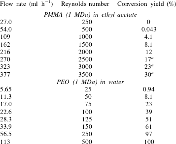
where $\unicode[STIX]{x1D70C}$ and $\unicode[STIX]{x1D702}$ are the solvent density and viscosity, $Q$ is the volumetric flow rate, and $D$ is the diameter of the outlet. To trigger chain scission, $Q$ has to be high in order to generate large extensional rates. On the other hand, $Re$ has to be kept limited to avoid turbulence. In our simulations, inertial instabilities usually appear above a Reynolds number of 2500. Simulations are done for the two types of polymer solutions (PMMA in ethyl acetate and PEO in water) and various flow rates. The conversion yield, defined by the ratio of the flux of broken molecules over the total solute flux at the outlet, is recorded at the steady state. Results are reported in table 2. For the PMMA solution, simulations suggest that it is not possible to get 100 % of conversion yield with a single pass in a laminar flow regime. However, a nearly complete degradation should be obtained for the PEO solution at a Reynolds number of 250. In the next paragraph, we turn our attention to the local scission rate.

Table 2.

Simulation cases and global result.

a Time-averaged value.

4.2 Scission zones

In order to describe the location of scission events, we look at two situations: the PMMA solution at $Re=2000$ and the PEO at $Re=100$ . Results for a steady state flow are reported in figure 6. For the PMMA solution, the map of the scission rate, $k$ (figure 6 a), shows that the polymer breaks close to the sharp corner, upstream from the contraction. The maps of the conversion factor, $1-c^{+}$ , which is the proportion of broken chains (figure 6 b,c) confirm that a very large proportion of chains that flow through this region near the edge are broken. No rupture occurs along the centreline. By contrast, the PEO solution displays a different pattern. The scission zone spans across the entire entrance of the contraction (figure 6 d), which means some of the molecules flowing through the centre are damaged. This can be seen on the conversion maps (figure 6 e,f), where approximately 20 % of the chains are broken through the centreline. Like in the case of PMMA, every PEO molecules flowing near the sharp corner undergo chain scission.

Figure 6.

CFD results maps. (a–c) PMMA in ethyl acetate at $Re=2000$ ( $216~\text{ml}~\text{h}^{-1}$ ); (d–f) PEO in water at $Re=100$ ( $22.6~\text{ml}~\text{h}^{-1}$ ). (a,d) Scission rate ( $\text{s}^{-1}$ ); (b,c,e,f) conversion (scission) of initial polymer chains (shared scale bar).

4.3 Comparison with the molecular model

In order to discuss the consistency of the multiscale approach, the ensemble-averaged quantities given by both the CFD and bead–rod model are compared in the case of the PMMA solution at $Re=2000$ , along three streamlines. The paths and their starting points (time 0) are shown in figure 7. The corner streamline is chosen very close to the sharp edge so that a large portion of chains are broken; limit is a streamline where only a very limited amount of chain scissions occur; and centre is the centreline. The strain rate tensor extracted along the streamline with the velocity of a massless particle is given as input for the bead–rod model. 256 runs are done along the same particle path, each with a random initial configuration for the chain. This method provides ensemble-averaged quantities such as the mean normalised extension of the chain $\unicode[STIX]{x1D706}$ , and the ensemble-average force in the chains $\langle g\rangle$ , and ultimately the proportion of broken chains.

Results are shown in figure 8. Figure 8(a–c) compares $\unicode[STIX]{x1D706}$ in the two models. For the corner and limit trajectories, the agreement is good upstream from the capillary, but the bead–rod model exhibits a larger extension in the tube. The agreement is evident along the centreline (figure 8 c). This general behaviour can be explained by the fact that the constitutive equation (3.20) has been optimised to fit purely elongational flows, such as along the symmetry axis of the contraction, whereas significant vorticity is developed near the edge, reaching the characteristics of a shear flow. Another cause of deviation can be the numerical diffusion introduced by the discretisation scheme, which is likely to be particularly severe near the sharp edge.

Figure 7.

Three streamlines used for comparison with the bead–rod model, shown on top of the conversion factor (PMMA in ethyl acetate at $Re=2000$ ).

The internal tension in the chains $\langle g\rangle$ (figure 8 d–f) displays three different regimes in each streamline. Far upstream from the contraction, the tension from the bead–rod model starts from a lower bound about 0.02 nN, corresponding to thermal fluctuations only, whose impact is not present in the CFD model. Then the tension reaches a peak where both models are in agreement, and finally the models diverge downstream of the contraction. This difference can assumed to be caused again by vorticity, and also by a distinct tension dynamics in recoiling chains. To sum up, (3.16) provides a good macroscopic description of the bead–rod model for nearly unravelled chains under tension, which is often when mechanochemistry will occur.

Both models are in very good agreement (3 % difference) regarding the conversion factor, and predict about 63 % of chain scission along the corner streamline, as seen in figure 8(g). The CFD value is not monotonic but fluctuates due to interpolation between cells. On the other hand, the models do not match along the limit line (figure 8 h) for the following reasons:

1. (i) Low mesh resolution: in the CFD model, scissions occur in a small number of cells (figure 6 a), hence a too coarse description of the scission rate along this streamline.

2. (ii) Numerical diffusion: the conversion factor diffuses towards cells with less scission.

Nevertheless, this discrepancy should affect only a thin region of the simulation domain and, in particular, is not likely to disturb qualitative considerations (where the chains break and the influence of the device geometry), or global quantities that we now present below.

Figure 8.

Comparison between the bead–rod and CFD models (only the end of the trajectories are shown). (a–c) Normalised extension of the chains, $\unicode[STIX]{x1D706}$ . (d–f) Ensemble-averaged maximum tension $\langle g\rangle$ . (g,h) Conversion factor (no scission for the centreline in both models).

4.4 Critical flow rate

The threshold nature of polymer scission in strong flows has often been characterised by a critical elongational rate or a critical flow rate. In experiments, where measuring this threshold directly is subject to high noise, a linear interpolation of any changing properties such as the fluid viscosity or the conversion yield is made instead. The linear fit crosses the $x$ -axis at a critical flow rate, $Q_{c}$ . The simulations described in table 2 show the same phenomenon, and a linear fit is possible below a conversion of up to 30–60 %, as shown in figure 9. According to the simulations of this 80- $\unicode[STIX]{x03BC}\text{m}$ -diameter contraction, the critical flow rates are $Q_{c}=65\pm 10~\text{ml}~\text{h}^{-1}$ for 1 MDa PMMA in ethyl acetate, and $Q_{c}=4\pm 1~\text{ml}~\text{h}^{-1}$ for 1 MDa PEO in water. The rather high uncertainty on the interpolated value of $Q_{c}$ from the linear fit suggests that this method only indicates the order of magnitude of the critical flow rate.

Nevertheless, this type of curve provides a method to calibrate the model by tuning parameters (such as the bead friction $\unicode[STIX]{x1D701}$ or the critical tension $g_{c}$ ) to fit simple scission experiments with controllable flow rate. In this way, accurate quantitative predictions could be obtained for transient and more complex flows.

Figure 9.

Conversion yield as a function of flow rate, and linear fit defining the critical flow rate. (a) PMMA in ethyl acetate; (b) PEO in water.

4.5 Mesh sensitivity

The Newtonian flow around a sharp re-entrant corner has a singular velocity gradient which is improperly captured by a finite size mesh (Dean & Montagnon Reference Dean and Montagnon1949). Since the chain unravelling dynamics and scission rate computation depend on the velocity gradient, the robustness of the model upon mesh resolution should be tested. For this purpose, the initial mesh (78 000 cells) used so far in this paper is recursively coarsened to give three additional meshes with 18 000, 4500 and 1125 cells, respectively. The chain scission simulations of PMMA in ethyl acetate are computed again on these meshes and results for the conversion yield (percentage of broken chains) are reported in figure 10.

Below $200~\text{ml}~\text{h}^{-1}$ , the cell resolution affects the quantitative result to a large extent, but the four meshes predict a non-zero conversion above $100~\text{ml}~\text{h}^{-1}$ ; the finest mesh alone predicts a non-zero conversion at $54~\text{ml}~\text{h}^{-1}$ . On the other hand, above $200~\text{ml}~\text{h}^{-1}$ only the coarsest mesh differs significantly from the reference, while the relative gaps with the 18k-cell and 4.5k-cell meshes quickly fall down to a few percent (figure 10 b). This consistency at high conversion yield can be explained by the saturating first-order dynamics of chain scission. The region near the corner where the mesh resolution has the most influence on the velocity gradient magnitude is also the place where the local conversion is already close to 100 %. A scission rate locally increased by mesh refinement would only cause a faster conversion for chains approaching the corner, but the final yield through this region would still saturate at 100 %.

In summary, if very small conversion yields are the primary interest, then the effort should be placed on the accurate description of the corner, especially for comparison with manufactured channels of finite resolution. On the other hand, the model shows an acceptable robustness upon mesh coarsening for higher conversion yields, even in the presence of a sharp corner.

Figure 10.

Mesh sensitivity results for the conversion yield of PMMA in ethyl acetate. (a) Conversion yields. (b) Relative difference to the reference mesh (78 000 cells).