


1. Introduction
The flow around bluff bodies positioned transversely near a planar wall has garnered significant interest in fluid mechanics due to its fundamental and practical importance (Squire Reference Squire1989; Ovchinnikov, Piomelli & Choudhari Reference Ovchinnikov, Piomelli and Choudhari2006; Maiti Reference Maiti2012; Malavasi & Blois Reference Malavasi and Blois2012; Kukreti & Singh Reference Kukreti and Singh2023). However, notable differences exist in the simplified models of blunt bodies across various engineering applications. For instance, the subsea oil and gas pipelines are often modelled as circular cylinders in proximity to a wall, whereas vehicles such as cars and trains, as well as some buildings, are typically represented as elongated rectangular cylinders near a wall. The flow characteristics around a rectangular cylinder differ markedly from those around a circular cylinder, with the former exhibiting phenomena such as shear layer separation and subsequent reattachment (Cimarelli et al. 2018a, 2019a; Chiarini & Quadrio Reference Chiarini and Quadrio2021), which are less pronounced in flows involving circular geometries. Consequently, understanding the vortex dynamics in the flow around near-wall bluff bodies is crucial for elucidating fundamental aspects of fluid mechanics. The present study primarily investigates the flow characteristics around a near-wall rectangular cylinder (FNRC), exploring the influence of near-wall effects on the flow around the rectangular cylinder.
The interaction between the wake of a circular cylinder and the boundary layer of a plate wall has been extensively studied in both experimental (Bearman & Zdravkovich Reference Bearman and Zdravkovich1978; Zdravkovich Reference Zdravkovich1985; Lei, Cheng & Kavanagh Reference Lei, Cheng and Kavanagh1999; Price et al. Reference Price, Sumner, Smith, Leong and Paidoussis2002; Wang & Tan Reference Wang and Tan2008; He, Pan & Wang Reference He, Pan and Wang2013a
, Reference He, Wang, Pan, Feng, Gao and Rinoshika2017; Wang, He & Wang Reference Wang, He and Wang2024) and numerical simulations (Lei et al. Reference Lei, Cheng, Armfield and Kavanagh2000; Sarkar & Sarkar Reference Sarkar and Sarkar2009, Reference Sarkar and Sarkar2010; Ouro, Muhawenimana & Wilson Reference Ouro, Muhawenimana and Wilson2019; Chen et al. Reference Chen, Ji, Alam, Xu and Zhang2022; Li et al. Reference Li, Wang, Qiu, Wu, Zhou, Fu and Liu2022a,b). These investigations reveal that the flow around a near-wall circular cylinder (FNCC) is primarily influenced by several key parameters, including the gap ratio
 $G/D$
(where
 $G$
is the distance from the wall to the bottom side of the cylinder and
 $D$
is the cylinder thickness), the Reynolds number
 $Re = U_0 D/\nu$
(with
 $U_0$
as the fixed free stream velocity outside the plate boundary layer and
 $\nu$
as the kinematic viscosity) and the plate boundary layer thickness
 $\delta _D/D$
(where
 $\delta _D$
is the boundary layer thickness at the position of the cylinder in the absence of the cylinder). Among these parameters,
 $G/D$
is particularly critical, as it governs the vortex dynamics of the FNCC.
A prominent phenomenon observed in the FNCC in the subcritical regime of
 $Re \sim 10^{3}\!-\!10^{5}$
is the induction of plate boundary layer separation by the wake vortex at certain gap ratios, leading to the formation of a secondary vortex (SV) structure that rotates in the same direction as the upper wake vortex. The interaction between the wake vortex and the SV is significantly influenced by
 $G/D$
. For
 $G/D \leqslant 0.125$
, the alternate vortex shedding from the upper and lower sides of the cylinder is suppressed (Price et al. Reference Price, Sumner, Smith, Leong and Paidoussis2002; Li et al. Reference Li, Wang, Qiu, Wu, Zhou, Fu and Liu2022a
). Price et al. (Reference Price, Sumner, Smith, Leong and Paidoussis2002) noted the presence of periodicity in the upper shear layer, despite the absence of regular vortex shedding. This periodicity has been attributed to the Kelvin–Helmholtz (KH) instability in the upper shear layer, resulting in the formation of KH vortices, as demonstrated in the study by Li et al. (Reference Li, Wang, Qiu, Wu, Zhou, Fu and Liu2022a
). Furthermore, Li et al. (Reference Li, Wang, Qiu, Wu, Zhou, Fu and Liu2022a
) observed that the KH vortex evolves into hairpin vortices downstream due to secondary instability. For the range
 $0.25 \leqslant G/D \leqslant 0.5$
, the SV forms from the wall boundary layer as a result of the wake vortex induction. This is followed by complex interactions among the upper wake vortex, the lower wake vortex and the SV (Price et al. Reference Price, Sumner, Smith, Leong and Paidoussis2002; Sarkar & Sarkar Reference Sarkar and Sarkar2009, Reference Sarkar and Sarkar2010; He et al. Reference He, Wang, Pan, Feng, Gao and Rinoshika2017; Li et al. Reference Li, Wang, Qiu, Wu, Zhou, Fu and Liu2022a
; Zhou et al. Reference Zhou, Qiu, Li and Liu2022). During these interactions, the lower wake vortex breaks up, while the SV rises and merges with the upper wake vortex. This merging leads to the development of hairpin vortices and braid vortices (Li et al. Reference Li, Wang, Qiu, Wu, Zhou, Fu and Liu2022a
). In the range
 $0.7 \leqslant G/D \leqslant 1.0$
, the interactions between vortices diminish, as the SV interacts only with the lower wake vortex, leaving the upper wake vortex uninvolved (Price et al. Reference Price, Sumner, Smith, Leong and Paidoussis2002; He et al. Reference He, Pan and Wang2013a
,Reference He, Wang and Pan
b
; Li et al. Reference Li, Wang, Qiu, Wu, Zhou, Fu and Liu2022a
). Additionally, the hairpin vortex evolves from the SV, but its head becomes entrained into the wake (Li et al. Reference Li, Wang, Qiu, Wu, Zhou, Fu and Liu2022a
). As the gap ratio increases to
 $G/D = 2-3$
, the SV can still form periodically. However, there is no direct interaction between the SV and the wake vortices. The SV can also develop into hairpin vortices (He et al. Reference He, Pan, Feng, Gao and Wang2016, Reference He, Wang, Pan, Feng, Gao and Rinoshika2017). During these varying interactions, Li et al. (Reference Li, Wang, Qiu, Wu, Zhou, Fu and Liu2022a
) identified a tertiary vortex (TV), which is induced by the SV and rotates in the opposite direction. Notably, the characteristic frequency
 $f$
of the TV matches that of the wake vortices along with the SV. Recently, Jiang et al. (Reference Jiang, Ju, Guo and Wang2024) investigated the flow around a circular cylinder in proximity to a moving wall for
 $Re = 300-1000$
and
 $G/D = 0.2-3$
. The moving wall eliminates the boundary layer while retaining a near-wall effect, thereby elucidating several flow characteristics documented in the literature for a stationary wall. By comparing flows between stationary and moving walls, they found that the development of the upstream wall boundary layer significantly affects the flows, particularly leading to an increase in the Strouhal number
 $St = {fD}/{U_0}$
for a stationary wall for
 $G/D = 0.5-2$
.
Compared with the flow around a circular cylinder, the flow around a rectangular cylinder introduces an additional parameter: the aspect ratio
 $L/D$
(where
 $L$
represents the streamwise dimension of the rectangular cylinder). The flow around an isolated rectangular cylinder (FIRC) exhibits distinct features depending on the value of
 $L/D$
and has garnered significant interest from researchers over the years. When
 $L/D$
is sufficiently large (
 $L/D \gt 3$
), the shear layer developing from the leading edge (LE) can reattach to the upper and lower sides of the rectangular cylinder, resulting in flow separation at the trailing edge (TE). Consequently, the LE vortices and TE vortices can form separately for
 $Re \gt 300$
. Notably, the shedding frequency of these vortices is the same, indicating a phenomenon known as frequency locking, which is a key characteristic of vortex dynamics in the flow around a rectangular cylinder. In the FIRC, two distinct increases in the new Strouhal number
 $St(L) = fL/U_0$
are observed as
 $L/D$
increases. The first increase occurs in a stepwise manner, dominated by the LE vortex (Okajima Reference Okajima1982; Nakamura, Ohya & Tsuruta Reference Nakamura, Ohya and Tsuruta1991; Ozono et al. Reference Ozono, Ohya, Nakamura and Nakayama1992; Mills et al. Reference Mills, Sheridan, Hourigan and Welsh1995; Tan, Thompson & Hourigan Reference Tan, Thompson and Hourigan1998; Chiarini et al. Reference Chiarini, Quadrio and Auteri2022c
; Zhang et al. Reference Zhang, Kareem, Xu and Jiang2023). In contrast, the second increase of
 $St(L)$
rises almost linearly with
 $L/D$
(Chiarini et al. Reference Chiarini, Quadrio and Auteri2022c
). To elucidate the frequency locking and the stepwise dependence of
 $St(L)$
, studies on the impinging shear layer instability (Nakamura & Nakashima Reference Nakamura and Nakashima1986) and the impinging LE vortex instability (Nakamura et al. Reference Nakamura, Ohya and Tsuruta1991; Naudascher & Rockwell Reference Naudascher and Rockwell1994; Mills, Sheridan & Hourigan Reference Mills, Sheridan and Hourigan2002; Tan, Thompson & Hourigan Reference Tan, Thompson and Hourigan2004; Chiarini et al. Reference Chiarini, Quadrio and Auteri2022c
) have been conducted, respectively. Recently, Chiarini, Quadrio & Auteri (Reference Chiarini, Quadrio and Auteri2021) identified that the primary instability is attributed to a Hopf bifurcation at low
 $Re$
. Furthermore, Chiarini et al. (Reference Chiarini, Quadrio and Auteri2022b
) discovered a new quasisubharmonic unstable mode at
 $L/D = 5$
, with the wavemaker region located on the upper and lower sides of the rectangular cylinder. This three-dimensional (3-D) instability arises from the mutual inviscid interaction of vortices originating from the LE shear layer. Moreover, Zhang et al. (Reference Zhang, Kareem, Xu and Jiang2023) concentrated on global instability and identified the phase difference between the LE and TE vortices as a critical factor contributing to the stepwise growth of
 $St(L)$
as
 $L/D$
increases. They demonstrated that self-sustained oscillations are maintained by two types of pressure feedback-loop mechanisms (Hourigan, Thompson & Tan Reference Hourigan, Thompson and Tan2001): the flow exhibits the impinging shear layer instability at
 $L/D = 4$
and
 $5$
, while it is characterized by the impinging LE vortex instability for
 $L/D = 3$
and
 $6$
–
 $12$
.
Regarding the vortex dynamics of the flow around a rectangular cylinder, Chiarini et al. (Reference Chiarini, Quadrio and Auteri2022c
) identified that the shedding dynamics of the TE vortex are pivotal in the phenomenon of frequency locking at
 $Re=400$
. They found two distinct configurations in the two-dimensional flow, which exhibit a significant correlation with the interaction between the LE and TE vortices. At a medium Reynolds number (
 $Re=1000$
), Li et al. (Reference Li, Wang, Qiu, Zhou, Fu and Liu2024b
) discovered a fractional harmonic in the 3-D flow, revealing that it arises from the feedback effect resulting from the interaction between the reverse boundary layer and the upstream development of the split LE shear layer. They also identified two shedding patterns – ipsilateral and contralateral vortex shedding – at different
 $L/D$
, similar to the configurations found by Chiarini et al. (Reference Chiarini, Quadrio and Auteri2022c
). Notably, contralateral vortex shedding can suppress Kármán-type vortex development in the wake. Additionally, Li et al. (Reference Li, Wang, Qiu, Zhou, Fu and Liu2024a
) further evaluated the connection between crucial vortices and turbulent transport. For high Reynolds numbers (
 $Re \geqslant 3000$
), previous studies have predominantly focused on the flow for
 $L/D=5$
. This flow is characterized by quasistreamwise vortices and streamwise streaks on the upper and lower sides (Cimarelli et al. Reference Cimarelli, Leonforte and Angeli2018b). The self-sustaining mechanisms of the flow have been derived, showing that large-scale pressure fluctuations alternate between promoting and suppressing the reverse flow. Driven by large-scale dynamics, small-scale motions trigger the LE shear layer, which subsequently creates vortices that alternate between the upper and lower sides of the cylinder, resulting in a relatively long period of inversion and thus closing the self-sustaining cycle. Cimarelli et al. (Reference Cimarelli, Leonforte, Angelis, Crivellini and Angeli2019a
,Reference Cimarelli, Leonforte, Angelis, Crivellini and Angeli
b
), Chiarini & Quadrio (Reference Chiarini and Quadrio2021) and Chiarini et al. (Reference Chiarini, Quadrio and Auteri2022a
) also studied spatial and interscale energy transport to understand the evolutionary behaviour of turbulent vortex structures. Furthermore, Cimarelli, Corsini & Stalio (Reference Cimarelli, Corsini and Stalio2024) provided a detailed analysis of this flow at
 $Re=3000$
,
 $8000$
and
 $14\,000$
, encompassing the laminar boundary layer on the front face, the separated shear layer, flow impingement at reattachment, the reverse boundary layer and near- and far-wake flow. The physics of these phenomena are elaborated, including the slow modulation induced by large-scale instabilities associated with vortex shedding. The literature review suggests that the flow around a rectangular cylinder exhibits more diverse flow features than that around a circular cylinder, garnering considerable attention in the research community.
The FNRC is commonly encountered in engineering applications, as previously described. However, most prior research focused on circular cylinders when examining bluff bodies near a wall. Additionally, the near-wall effect on the vortex dynamics in the FNRC is expected to be more complex. Although some studies have been conducted on this flow, most have concentrated on configurations where
 $0.1 \leqslant L/D \leqslant 2$
(Maiti Reference Maiti2012; Tanweer et al. Reference Tanweer, Dewan and Sanghi2021, Reference Tanweer, Dewan and Sanghi2022). Recently, Chiarini & Auteri (Reference Chiarini and Auteri2023) investigated the primary instability of the steady two-dimensional flow past rectangular cylinders moving parallel to a wall at
 $Re \leqslant 300$
, neglecting the influence of the wall boundary layer. Consequently, the vortex dynamics of the FNRC warrants further investigation, particularly in terms of its similarities and differences with the FNCC and FIRC.
In this work, we delve into the vortex dynamics in the flow around a rectangular cylinder positioned near a plate, including the intricate interactions between the plate boundary layer and the LE/TE vortex shed from the rectangular cylinder. To the best of the authors’ knowledge, such research has not been previously reported. The investigation is conducted using direct numerical simulation (DNS) at a medium Reynolds number
 $(Re=1000$
). Three aspect ratios (
 $L/D=5$
,
 $10$
and
 $15$
) and gap ratios (
 $G/D=0.1$
,
 $0.3$
and
 $0.9$
) are considered. This study is expected to enhance the physical understanding of vortex dynamics, thereby improving insights into the flow physics around a near-wall blunt body. The structure of the paper is organized as follows:
 $\S$
2 presents the physical model, numerical methods, and data analysis techniques; the main findings are discussed in
 $\S$
3; finally,
 $\S$
4 provides the conclusions drawn from this study.
2. Numerical model
2.1. Flow configuration and numerical method
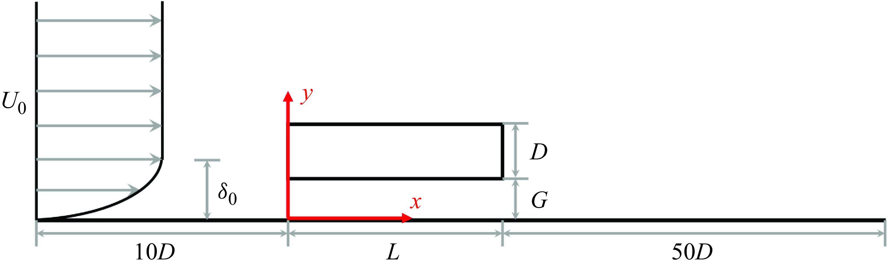
In the present study, 3-D DNS are performed to investigate the flow around a rectangular cylinder positioned transversely near a plate wall. The sketch of this flow configuration is presented in figure 1, where
 $L$
and
 $D$
represent the streamwise and wall-normal dimensions of the rectangular cylinder, respectively, and
 $G$
denotes the gap between the plate wall and the lower side of the cylinder. Following the studies of Li et al. (Reference Li, Wang, Qiu, Wu, Zhou, Fu and Liu2022a
) and Li et al. (Reference Li, Wang, Qiu, Zhou, Fu and Liu2024b
), the computational domain is defined as
 $ -10D \leqslant x \leqslant L + 50D$
in the streamwise direction,
 $0\leqslant y \leqslant 15D$
in the wall-normal direction and
 $ 0 \leqslant z \leqslant 2\pi D$
in the spanwise direction. To explore the near-wall effect on the flow and to compare the vortex dynamics with that in the FNCC (Li et al. Reference Li, Wang, Qiu, Wu, Zhou, Fu and Liu2022a
) and FIRC (Li et al. Reference Li, Wang, Qiu, Zhou, Fu and Liu2024b
), the Reynolds number is fixed at
 $1000$
. The study considers three aspect ratios (
 $L/D = 5, 10, 15$
) and small gap ratios (
 $G/D = 0.1, 0.3, 0.9$
). The governing equations consist of the continuity and incompressible Navier–Stokes equations in their dimensionless form, expressed as follows:
 \begin{equation} \nabla \cdot \textbf{u}=0, \end{equation}
 \begin{equation} \frac {\partial \textbf{u}}{\partial t}+\textbf{u}\cdot \bigtriangledown \textbf{u}=-\nabla p+\frac {1}{Re}\nabla ^{2}\textbf{u}, \end{equation}
The sketch of FNRC in a
 $x{-}y$
plane. Here
 $L$
and
 $D$
are the streamwise and wall-normal dimensions of the rectangular cylinder. The gap
 $G$
is the distance from the wall to the bottom side of the cylinder. Here
 $U_0$
is the inflow velocity;
 $\delta _0$
is the wall boundary layer thickness at the inlet.

where,
 $\textbf{u}\equiv (u,v,w)$
is velocity vector,
 $t$
is time and
 $p$
is pressure. The Reynolds number is also defined as
 $Re=U_0 D/\nu$
, where
 $D$
is the cylinder thickness and
 $U_0$
is the free stream streamwise velocity outside the plate boundary layer. Equations (2.1) and (2.2) are solved using the unsteady incompressible Navier–Stokes solver embedded in the open-source code Nektar++ (Cantwell et al. Reference Cantwell2015; Moxey et al. Reference Moxey2020). This solver utilizes the Fourier spectral/hp element method (Bolis Reference Bolis2013) and has been widely employed in studies of flow around bluff bodies (Ju et al. Reference Ju, An, Cheng and Tong2020; Jiang et al. Reference Jiang, Hu, Cheng and Zhou2022; Li et al. Reference Li, Li, Wu, Chong, Wang, Zhou and Liu2023; Ren et al. Reference Ren, Liu, Cheng, Tong and Xiong2023; Ju & Jiang Reference Ju and Jiang2024).
A laminar flow profile, based on the Blasius similarity solution, is imposed at the inlet (Li et al. Reference Li, Wang, Qiu, Wu, Zhou, Fu and Liu2022a,b; Feng et al. Reference Feng, Tu, Yang, Wang, Zhou and Chen2024), resulting in a boundary layer thickness of
 $\delta _0 = 0.492D$
. The far field conditions, defined as
 $\partial u/\partial y=0$
,
 $v = 0$
and
 $\partial w/\partial y = 0$
, are applied along the upper surface of the computational domain. No-slip boundary conditions (
 $u = v = w = 0$
) are enforced on the surfaces of the rectangular cylinder and the plate wall (the lower surface of the domain). At the outlet, a high-order outflow boundary condition is implemented (Dong, Karniadakis & Chryssostomidis Reference Dong, Karniadakis and Chryssostomidis2014). A second-order implicit–explicit time integration scheme is chosen from the incompressible solver, and the time step is fixed at
 $0.001$
. The problem is spatially discretized in the
 $x{-}y$
plane, combined with the Fourier expansion in the
 $z$
direction to capture the 3-D characteristics of the flow, based on the assumption of homogeneity in the spanwise direction (Bolis Reference Bolis2013). In the spanwise direction,
 $N = 96$
Fourier planes are utilized, as referenced in the studies by Li et al. (Reference Li, Wang, Qiu, Wu, Zhou, Fu and Liu2022a) and Li et al. (2024b) with the same
 $Re$
. In the
 $x{-}y$
plane, the spatial resolution is determined by the distribution of
 $h$
-type elements, and the macromesh for
 $L/D=5$
,
 $G/D=0.3$
is shown in figure 2
 $(a)$
.
 $(a)$
The partial domain with a macro mesh for
 $L/D=5$
,
 $G/D=0.3$
in the
 $x{-}y$
plane. The inset is a close-up view of the mesh near the rectangular cylinder.
 $(b)$
The ratio of the grid size to the Kolmogorov length scale (
 $\unicode{x1D6E5} /\eta$
) in the
 $x{-}y$
plane for
 $L/D=5$
and
 $G/D=0.3$
.

The reliability of Nektar++ has been well-established in previous studies of the FNCC (Li et al. Reference Li, Wang, Qiu, Wu, Zhou, Fu and Liu2022a
,b) and FIRC (Li et al. Reference Li, Wang, Qiu, Zhou, Fu and Liu2024a
,Reference Li, Wang, Qiu, Zhou, Fu and Liu
b
) at
 $Re=1000$
. In this study, the FNRC is investigated for the first time with a large
 $L/D$
. To ensure the accuracy of the numerical results, a mesh independence study is conducted by evaluating the convergence of the drag coefficient
 $C_D = 2F_x / \rho D U_0^2$
and the lift coefficient
 $C_L = 2F_y / \rho L U_0^2$
, where
 $F_x$
and
 $F_y$
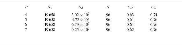
represent the spanwise-averaged total forces acting on the cylinder in the streamwise and wall-normal directions, respectively. The mean drag and lift coefficients (
 $\overline {C_D}$
and
 $\overline {C_L}$
) for different polynomial orders
 $P$
are presented in table 1, using the typical case of
 $L/D = 5$
and
 $G/D = 0.3$
. Four meshes are generated with
 $P$
(the order interpolation polynomials for the
 $p$
-type expansion) varying from
 $4$
to
 $7$
. It can be observed that
 $\overline {C_D}$
and
 $\overline {C_L}$
show good convergence as
 $P$
increases.
Time-averaged drag coefficient
 $\overline {C_D}$
and lift coefficient
 $\overline {C_L}$
of the rectangular cylinder with different orders of polynomial expansion
 $P$
at
 $L/D=5$
and
 $G/D=0.3$
. Here
 $N_v$
is the number of elements,
 $N_d$
is approximate degree of freedom and
 $N$
is the number of Fourier planes.

The time- and spanwise-averaged pressure coefficient profiles
 $C_p$
 $(a)$
and skin friction coefficient profiles
 $C_f$
 $(b)$
on the surface of the rectangular cylinder for various values of
 $P$
at
 $L/D=5$
,
 $G/D=0.3$
.

Meanwhile, the ratio of the grid size to the Kolmogorov length scale (
 $\unicode{x1D6E5} /\eta$
) is investigated here. The grid size,
 $\unicode{x1D6E5}$
, is determined based on the maximum dimension of a grid cell in all three directions, specifically
 $\unicode{x1D6E5} = \max (\unicode{x1D6E5} _{x}, \unicode{x1D6E5} _{y}, \unicode{x1D6E5} _{z})$
. The Kolmogorov length scale is calculated using the formula
 $\eta = (\nu ^{3}/\varepsilon )^{1/4}$
, where
 $\varepsilon$
is the local dissipation rate. According to the findings of the studies by Moser & Moin (Reference Moser and Moin1987), Zhou et al. (Reference Zhou, Nagata, Sakai, Ito and Hayase2015), Zhou et al. (Reference Zhou, Nagata, Sakai and Watanabe2019) and Mahmoodi-Jezeh & Wang (Reference Mahmoodi-Jezeh and Wang2020), it is crucial for the grid size to be of the same order as the Kolmogorov length scale, i.e.
 $ O(\unicode{x1D6E5} /\eta ) \sim O(1)$
, to accurately capture the turbulence kinetic energy dissipation associated with the smallest scales of turbulence. The distribution of
 $\unicode{x1D6E5} /\eta$
for the typical case of
 $L/D=5$
and
 $G/D=0.3$
is illustrated in figure 2
 $(b)$
. The results show that
 $\unicode{x1D6E5} /\eta$
is generally less than
 $5$
, indicating that
 $\unicode{x1D6E5} /\eta = O(1)$
. This confirms that the grid spacing is adequate for accurately performing DNS of turbulent flows. Furthermore, the time- and spanwise-averaged pressure coefficient
 $C_p$
and skin friction coefficient
 $C_f$
on the surface of a rectangular cylinder are investigated, which are given by
 \begin{equation} C_p=\frac {\bar {p}-\bar {p}_{ref}}{0.5\rho U_0^2},\quad C_f=\frac {\tau _w}{0.5\rho U_0^2}, \end{equation}
where
 $\bar {p}$
and
 $\bar {p}_{ref}$
are the mean surface pressure and the reference pressure, respectively, and
 $\tau _w$
is the mean shear stress. The profiles of
 $C_p$
and
 $C_f$
for various values of
 $P$
at
 $L/D=5$
,
 $G/D=0.3$
are shown figures 3
 $(a)$
and 3
 $(b)$
, respectively. It can be observed that for different values of
 $P$
, the
 $C_p$
and
 $C_f$
profiles on the lower surface of the rectangular cylinder nearly coincide. However, on the upper surface, both
 $C_p$
and
 $C_f$
are influenced by variations in
 $P$
. Beyond
 $\textrm {for}\, x/D \gt 3.5$
, the
 $C_p$
and
 $C_f$
at
 $P = 4$
exhibit a slight deviation from the other values of
 $P$
for
 $x/D \gt 3.5$
. In contrast, for
 $P \geqslant 5$
, the
 $C_p$
and
 $C_f$
curves almost entirely overlap, indicating a stronger convergence. Thus, it is concluded that
 $P = 5$
and
 $N = 96$
are sufficient for the current simulations.
Once the flow reaches a statistically steady state, statistical data are accumulated at each time step throughout the simulation for further
 $200D/U_0$
, and the sampling interval for the instantaneous 3-D flow field is set to
 $0.25D/U_0$
, which also defines the time interval for signal sampling at the spatial points (Li et al. Reference Li, Wang, Qiu, Zhou, Fu and Liu2024b
).
2.2. Data analysis techniques
2.2.1. Visualization of Lagrangian coherent structures
The finite-time Lyapunov exponents (FTLEs) method (Haller & Yuan Reference Haller and Yuan2000; Haller Reference Haller2001; Shadden, Dabiri & Marsden Reference Shadden, Dabiri and Marsden2006; Green, Rowley & Haller Reference Green, Rowley and Haller2007; Shadden, Astorino & Gerbeau Reference Shadden, Astorino and Gerbeau2010; He et al. Reference He, Wang, Pan, Feng, Gao and Rinoshika2017; Wang et al. Reference Wang, Gao, Wei and Wang2017, Reference Wang, Feng, Wang and Li2018; Wang & Wang Reference Wang and Wang2021a
; Li et al. Reference Li, Wang, Qiu, Zhou, Fu and Liu2024b
) and virtual dye visualization (He et al. Reference He, Pan, Feng, Gao and Wang2016; Wang & Wang Reference Wang and Wang2021b
; Cheng et al. Reference Cheng, Jiang, Chong, Zhou, Liu and Lu2022; Dong et al. Reference Dong, Pan, Tong and Yuan2024) serve as powerful tools for effectively tracking Lagrangian coherent structures (LCSs) in complex flows. Specifically, the flow map is defined as
 $\Phi _{t_0}^{t_{0}+t_{\unicode{x1D6E5}} } : \textbf{x}(t_0) \longrightarrow \textbf{x}(t_0+t_{\unicode{x1D6E5}})$
, which describes the mapping of fluid particles from their initial position
 $\textbf{x}(t_0)$
at time
 $t_0$
to their new position
 $\textbf{x}(t_0+t_{\unicode{x1D6E5}} )$
at
 $t_0+t_{\unicode{x1D6E5}}$
. The FTLE at
 $t_0$
can be calculated as follows:
 \begin{equation} \sigma (\textbf{x},t_0,t_{\unicode{x1D6E5}} )=\frac {1}{\left | 2t_{\unicode{x1D6E5}} \right | }ln\left ( \lambda _{max}\left \{ \left [\frac {\partial \textbf{x}(t_0+t_{\unicode{x1D6E5}} ) }{\partial \textbf{x}(t_0)} \right ]^T \left [ \frac {\partial \textbf{x}(t_0+t_{\unicode{x1D6E5}} )}{\partial \textbf{x}(t_0)} \right ] \right \} \right ). \end{equation}
In this context,
 $\sigma (\textbf{x}, t_0, t_{\unicode{x1D6E5}} )$
represents the exponential growth rate of nearby trajectories over a finite time interval
 $t_{\unicode{x1D6E5}}$
, while
 $\lambda _{\text{max}}$
denotes the largest singular value of the deformation gradient matrix. The integration can be conducted forward (
 $t_{\unicode{x1D6E5}} \gt 0$
) or backward (
 $t_{\unicode{x1D6E5}} \lt 0$
), resulting in FTLE ridges that exhibit repelling or attracting properties, respectively. The attracting property is employed for the extraction of LCSs, whereas the repelling property is utilized for virtual dye visualization.
2.2.2. Dynamic mode decomposition analyses
Dynamic mode decomposition (DMD) (Schmid Reference Schmid2010) is a significant modal analysis tool that has been widely utilized in previous studies (He et al. Reference He, Pan and Wang2013b ; Pan et al. Reference Pan, Wang, Wang and Sun2017; Li et al. Reference Li, Wang, Qiu, Wu, Zhou, Fu and Liu2022a ; Liu et al. Reference Liu, Wang, Li, Tao and Qiu2022; Li et al. Reference Li, Wang, Qiu, Zhou, Fu and Liu2024b ). The DMD effectively extracts a set of modes from the original unsteady dynamic flow, with each mode corresponding to spatial structures in the flow field that are dominant at a specific frequency. Therefore, in this work, DMD will be applied to extract the dominant frequency modes from the flow field snapshots, allowing for a comprehensive understanding of the underlying dynamics. The snapshots of the flow fields can be decomposed as follows:
 \begin{equation} \Phi (\textbf{x},t)=\textbf{U}(\textbf{x})+\sum _{k=1}^{r}b_k\phi _k(\textbf{x}) e^{\omega _k t}, \end{equation}
where
 $\Phi$
represents the reconstructed field and
 $\textbf{U}$
denotes the mean field. The terms
 $\phi _k$
and
 $b_k$
correspond to the
 $k$
th DMD mode and its associated magnitude, respectively. In the present study, the DMD analysis is conducted on 3-D flow fields, with each sample consisting of the three velocity components.
3. Results and discussion
3.1. Instantaneous 3-D vortices and statistics characteristics
In this section, the visualization of instantaneous vortical structures are presented first. Then, this section examines the effects of the aspect ratio
 $L/D$
and the gap ratio
 $G/D$
on the mean flow statistics, specifically focusing on the mean field topology, the scales of separation bubbles, and fluctuations. These characteristics will provide a comprehensive overview of vortex generation and evolution in the FNRC and will serve as a basis for analysing the near-wall effects on vortex dynamics in
 $\S$
3.2.
3.1.1. Instantaneous 3-D vortex structures
Instantaneous 3-D vortical structures visualized by isosurfaces of
 $Q=0.1$
at
 $G/D=0.1$
, coloured with the instantaneous streamwise velocity
 $u/U_0$
:
 $(a)$
 $L/D=5$
;
 $(b)$
 $L/D=10$
;
 $(c)$
 $L/D=15$
.

Instantaneous 3-D vortical structures visualized by isosurfaces of
 $Q=0.1$
at
 $G/D=0.3$
, coloured with the instantaneous streamwise velocity
 $u/U_0$
:
 $(a)$
 $L/D=5$
;
 $(b)$
 $L/D=10$
;
 $(c)$
 $L/D=15$
.

The instantaneous 3-D vortex structures for all flows are identified by the criterion with
 $Q=0.1$
. Figure 4 illustrates the instantaneous vortices for
 $G/D=0.1$
. The FNRC exhibits distinct asymmetry compared with the FIRC (Zhang et al. Reference Zhang, Kareem, Xu and Jiang2023; Li et al. Reference Li, Wang, Qiu, Zhou, Fu and Liu2024b
) and aligns more closely with the FNCC (Li et al. Reference Li, Wang, Qiu, Wu, Zhou, Fu and Liu2022a
) with the same
 $G/D$
, featuring a turbulent boundary layer downstream rather than the wake of an isolated blunt body. The KH instability in the upper leading edge (ULE) shear layer results in the formation of a two-dimensional upper KH (UKH) vortex. The LE/TE shear layer is the structure that detaches from the LE/TE corner (Cimarelli et al. Reference Cimarelli, Leonforte and Angeli2018b
; Chiarini et al. Reference Chiarini, Quadrio and Auteri2021; Cimarelli et al. Reference Cimarelli, Corsini and Stalio2024; Li et al. Reference Li, Wang, Qiu, Zhou, Fu and Liu2024b
). Moreover, there is no flow separation at the lower leading edge (LLE), leading to the absence of the vortices in the gap. As illustrated in figure 4
 $(a)$
, for
 $L/D=5$
and
 $G/D=0.1$
, the near-wall effect causes the UKH vortices to form and merge farther downstream compared with the FIRC (Zhang et al. Reference Zhang, Kareem, Xu and Jiang2023; Li et al. Reference Li, Wang, Qiu, Zhou, Fu and Liu2024b
), resulting in a larger streamwise scale of the mean LLE recirculation (shown in § 3.1.2). The 3-D instability of the ULE vortex manifests downstream of the UTE, rather than on the upper side of the rectangular cylinder, highlighting a significant contrast with the flow characteristics observed in the FIRC (Zhang et al. Reference Zhang, Kareem, Xu and Jiang2023; Li et al. Reference Li, Wang, Qiu, Zhou, Fu and Liu2024b
). As the ULE vortices interact with the downstream reverse wall boundary layer, hairpin vortices eventually form. For
 $L/D = 10$
and
 $15$
, as shown in figures 4
 $(b)$
and 4
 $(c)$
, the UKH vortices interact with the reverse boundary layer on the upper cylinder surface, evolving into hairpin vortices. For all these three flows, upon reattachment to the plate, the flow transitions into a wall boundary layer, with hairpin vortex packets forming farther downstream.
For
 $G/D=0.3$
, the instantaneous 3-D vortical structures are shown in figure 5. The KH instability in the ULE shear layer is observed across all three flows, leading to the formation of KH vortices. The absence of vortical structures within the gap indicates significant suppression of the LLE shear layer. In contrast to
 $G/D=0.1$
, the lower trailing edge (LTE) shear layer extends from the LTE for
 $L/D=5$
and
 $L/D=10$
(in figure 5
 $a$
and 5
 $b$
). However, at
 $L/D=15$
, the LTE shear layer is negligible, as shown in figure 5
 $(c)$
. At
 $L/D=5$
, as shown in figure 5
 $(a)$
, the UKH vortex forms farther downstream on the upper side of the cylinder. Consequently, the merged UKH vortex undergoes 3-D instability and evolves into the ULE vortex downstream. No hairpin vortices are present on the upper side, similar to the flow at
 $G/D=0.1$
. However, at
 $L/D=10$
and
 $15$
(in figure 5
 $b$
and
 $c$
), hairpin vortex packets appear on the upper side, which contrasts with the flow at
 $G/D=0.1$
. Furthermore, the distribution of ULE vortices becomes more intricate. When the gap ratio increases to
 $G/D = 0.9$
, as shown in figure 6, the influence of the upstream wall boundary layer diminishes, leading to the formation of a distinct LLE shear layer. In the gap, vortices are observed across all three
 $L/D$
configurations, indicating that KH vortices shed from the LLE shear layer, unlike at
 $G/D=0.1$
and
 $0.3$
. Both the LTE and TSVs are identifiable and closely related to the LLE vortex. The complexity of the vortical structures on the upper side of the cylinder increases.
Instantaneous 3-D vortical structures visualized by isosurfaces of
 $Q=0.1$
at
 $G/D=0.9$
, coloured with the instantaneous streamwise velocity
 $u/U_0$
:
 $(a)$
 $L/D=5$
;
 $(b)$
 $L/D=10$
;
 $(c)$
 $L/D=15$
.

3.1.2. Mean flow characteristics
The presence of a strong shear layer induced by the plate wall results in pronounced mean shear characteristics near the rectangular cylinder. Consequently, an investigation of these mean shear characteristics is undertaken in this section. Exploiting the spanwise homogeneity, the mean shear tensor in the
 $x{-}y$
plane is decomposed, which provides a comprehensive assessment of all non-zero components of the 3-D mean strain rate tensor (
 $S_{xy}$
) (Fang & Tachie Reference Fang and Tachie2020),
 \begin{equation} S_{xy}=\begin{bmatrix} \displaystyle\frac {\partial U}{\partial x} & \displaystyle\frac {1}{2}\left(\displaystyle\frac {\partial U}{\partial y}+ \displaystyle\frac {\partial V}{\partial x}\right) \\[12pt] \displaystyle\frac {1}{2}\left(\displaystyle\frac {\partial U}{\partial y}+ \displaystyle\frac {\partial V}{\partial x}\right)& \displaystyle\frac {\partial V}{\partial y} \end{bmatrix} =\textbf{M} \begin{bmatrix} \sigma _1 & 0\\ 0 & \sigma _2 \end{bmatrix} \textbf{M}^T, \end{equation}
where
 $\sigma _1$
and
 $\sigma _2$
are eigenvalues of
 $S_{xy}$
, while
 $\textbf{M}$
denotes the matrix of eigenvectors of
 $S_{xy}$
. Due to the incompressibility and the spanwise homogeneity of the mean flow, it follows that
 $\sigma _1 + \sigma _2 = \partial U/\partial x +\partial V/\partial y =0$
. Consequently, it can be inferred that
 $\sigma _1 = -\sigma _2$
, with
 $\sigma _1$
defined as positive to represent the magnitude of principal stretching. The time- and spanwise-averaged streamwise velocity (
 $U/U_0$
) fields for different cases are presented in figures 7
 $(a,c,e)$
–9
 $(a,c,e)$
. Meanwhile, the fields of principal stretching
 $\sigma _1$
, which reflect the distribution of mean shear strength, are displayed in figures 7
 $(b,d,f)$
–9
 $(b,d,f)$
.
Time- and spanwise-averaged streamwise velocity
 $U/U_0$
in pseudocolour with the superimposition of streamlines for
 $G/D=0.1$
:
 $(a)$
 $L/D=5$
;
 $(c)$
 $L/D=10$
;
 $(e)$
 $L/D=15$
. The principal stretching
 $\sigma _1$
for
 $G/D=0.1$
:
 $(b)$
 $L/D=5$
;
 $(d)$
 $L/D=10$
;
 $(f)$
 $L/D=15$
. The cures in (b), (d) and (f) are the local streamlines.

Time- and spanwise-averaged streamwise velocity
 $U/U_0$
in pseudocolour with the superimposition of streamlines for
 $G/D=0.3$
:
 $(a)$
 $L/D=5$
;
 $(c)$
 $L/D=10$
;
 $(e)$
 $L/D=15$
. The insets in (a), (c) and (e) are the close-up views. The black arrow marks the clockwise recirculation, while the magenta ones mark the anticlockwise recirculation. The principal stretching
 $\sigma _1$
for
 $G/D=0.3$
:
 $(b)$
 $L/D=5$
;
 $(d)$
 $L/D=10$
;
 $(f)$
 $L/D=15$
. The cures in (b), (d) and (f) are the local streamlines.

For
 $G/D = 0.1$
, a recirculation zone forms upstream of the rectangular cylinder in all flow cases, as shown in figure 7
 $(a,c,e)$
. The streamwise scale of this recirculation, which exceeds
 $3.7D$
for all three flows, is significantly larger than the scale observed in the FNCC, where it is smaller than
 $2D$
(Li et al. Reference Li, Wang, Qiu, Wu, Zhou, Fu and Liu2022b). This scale can be determined by the location of the reattachment point of the recirculation. On the upper side of the cylinder, a LE recirculation forms, similar to the FIRC (Zhang et al. Reference Zhang, Kareem, Xu and Jiang2023; Li et al. Reference Li, Wang, Qiu, Zhou, Fu and Liu2024b
), but with no recirculation on the lower side, creating an asymmetry not seen in the FIRC (Cimarelli et al. Reference Cimarelli, Leonforte and Angeli2018b
; Chiarini et al. Reference Chiarini, Gatti, Cimarelli and Quadrio2022a
; Li et al. Reference Li, Wang, Qiu, Wu, Zhou, Fu and Liu2022a
; Zhang et al. Reference Zhang, Kareem, Xu and Jiang2023; Cimarelli et al. Reference Cimarelli, Corsini and Stalio2024). For
 $L/D = 5$
, the LE recirculation nearly spans the entire upper surface of the cylinder without a distinct reattachment point, differing from the FIRC (Cimarelli et al. Reference Cimarelli, Leonforte, Angelis, Crivellini and Angeli2019a
; Chiarini & Quadrio Reference Chiarini and Quadrio2021; Chiarini et al. Reference Chiarini, Quadrio and Auteri2021; Zhang et al. Reference Zhang, Kareem, Xu and Jiang2023; Li et al. Reference Li, Wang, Qiu, Zhou, Fu and Liu2024b
). Immediately downstream of the cylinder, only a LTE recirculation is observed, with a significant wall recirculation also present, similar to the FNCC (He et al. Reference He, Pan and Wang2013a
,Reference He, Wang and Pan
b
, Reference He, Wang, Pan, Feng, Gao and Rinoshika2017; Li et al. Reference Li, Wang, Qiu, Wu, Zhou, Fu and Liu2022b), but with a smaller streamwise scale across all
 $L/D$
configurations. This difference arises because KH instability in the upper shear layer in the FNCC develops farther downstream (Li et al. Reference Li, Wang, Qiu, Wu, Zhou, Fu and Liu2022a
). The distribution of recirculations resembles that in backward-facing step flows (Ma & Schröder Reference Ma and Schröder2017; Li et al. Reference Li, Zhang, Liu, Wu and Gao2020; Ma, Tang & Jiang Reference Ma, Tang and Jiang2020), suggesting that the FNCC shear layer is more stable than the UTE shear layer in the current FNRC at the same
 $G/D$
, mainly due to the absence of upstream vortex disturbances. At
 $L/D = 5$
, the LE recirculation connects with the downstream wall recirculation, forming a continuous recirculation zone, allowing fluid to return from the downstream region to the upper side upstream of the cylinder. As shown in figure 7
 $(b,d,f)$
, the upstream wall boundary layer, ULE shear layer and UTE shear layer (for
 $L/D = 10, 15$
) exhibit strong shear characteristics. The upstream wall boundary layer rises upon encountering the rectangular cylinder, contributing to the formation of the upstream recirculation.
As
 $G/D$
increases to
 $0.3$
, the upstream recirculation persists, accompanied by the downstream wall recirculation, as illustrated in figure 8. The gap flow significantly enhances, obstructing the connection between the wall recirculation and the TE, in contrast to
 $G/D = 0.1$
. For
 $L/D = 5$
, the LE recirculation covers nearly the entire upper surface, with a distinct reattachment point and two recirculations behind the cylinder, differing from
 $G/D = 0.1$
. For
 $L/D = 10$
and
 $15$
, only one LTE recirculation is observed, as depicted in figures 8(c) and 8(e). Compared with the FNCC (He et al. Reference He, Pan and Wang2013a,b, Reference He, Wang, Pan, Feng, Gao and Rinoshika2017; Li et al. Reference Li, Wang, Qiu, Wu, Zhou, Fu and Liu2022b), a novel feature is the occurrence of multiple flow separations at the downstream wall recirculation, as seen in the insets of figure 8(a,c,e). At
 $L/D = 5$
, only an anticlockwise recirculation is observed beneath the wall recirculation (marked by the magenta arrow). However, at
 $L/D = 10$
and
 $15$
, both anticlockwise (marked by the magenta arrow) and clockwise (marked by the black arrow) recirculations appear. The distributions of
 $\sigma _1$
in figure 8
 $(b,d,f)$
are similar to those at
 $G/D = 0.1$
, although the shear strength beneath the rectangular cylinder is slightly higher for all three cases at
 $G/D = 0.3$
.
At
 $G/D = 0.9$
, the upstream wall recirculation weakens, and the gap flow increases significantly, as shown in figure 9
 $(a,c,e)$
. Unlike at
 $G/D = 0.1$
and
 $0.3$
, a LLE recirculation forms, with both its streamwise and wall-normal scales smaller than those of the ULE recirculation, indicating the establishment of the LLE shear layer. The recirculation pair behind the cylinder, though not perfectly symmetrical, resembles that in the FIRC, with two distinct recirculations, signalling a diminished near-wall effect. As shown in figure 9
 $(b,d,f)$
, the upstream wall boundary layer lifting is reduced and no longer contacts the cylinder. Additionally, figure 9
 $(a,c,e)$
show a small clockwise recirculation (marked by the black arrow) beneath the LLE recirculation, suggesting that the LLE vortex induces wall boundary layer separation. The downstream wall recirculation persists, indicating continued separation of the downstream wall boundary layer, but its scale is significantly reduced.
Time- and spanwise-averaged streamwise velocity
 $U/U_0$
in pseudocolour with the superimposition of streamlines for
 $G/D=0.9$
:
 $(a)$
 $L/D=5$
;
 $(c)$
 $L/D=10$
;
 $(e)$
 $L/D=15$
. The insets in (a), (c) and (e) are the close-up views. The black arrow marks the clockwise recirculation. The principal stretching
 $\sigma _1$
for
 $G/D=0.9$
:
 $(b)$
 $L/D=5$
;
 $(d)$
 $L/D=10$
;
 $(f)$
 $L/D=15$
. The cures in (b), (d) and (f) are the local streamlines.

The quantified size of the ULE recirculation:
 $(a)$
the streamwise scale
 $x_r$
; and
 $(b)$
wall-normal scale
 $y_h$
, compared with these for the FIRC at the same
 $Re$
(Li et al. Reference Li, Wang, Qiu, Zhou, Fu and Liu2024b
), respectively.

 $(a)$
The local angle
 $ \theta$
between the ULE shear layer and the
 $x$
coordinate.
 $(b)$
The local principal stretching
 $\sigma _1$
along the ULE shear layer for
 $L/D=10$
and
 $15$
. The values for
 $L/D=15$
are increased by 10. The pentagrams represent the locations where the flows reattach.

Figures 7 to 9 show that the size of the ULE recirculation changes with increasing
 $G/D$
. The streamwise (
 $x_r$
) and wall-normal (
 $y_h$
) scales of the ULE recirculation are quantified in figures 10
 $(a)$
and 10
 $(b)$
, respectively, with comparison with the LE recirculation in the FIRC at the same
 $Re$
. Here
 $x_r$
is determined by the reattachment point, where the wall friction coefficient changes from a negative value to a positive value. Since the streamwise velocity is negative within the recirculation,
 $y_h$
is determined by the point with the maximum wall-normal position within the recirculation. For
 $L/D = 5$
, the ULE recirculation nearly covers the entire upper surface, resulting in a significantly larger
 $x_r$
compared with the FIRC (Li et al. Reference Li, Wang, Qiu, Zhou, Fu and Liu2024b
). As shown in figure 10
 $(a)$
, the streamwise scale
 $x_r$
for
 $L/D = 10$
and
 $15$
is also larger than in the FIRC, indicating that the near-wall effect delays reattachment. In contrast, the wall-normal scale
 $y_h$
, shown in figure 10
 $(b)$
, is smaller than in the FIRC (Li et al. Reference Li, Wang, Qiu, Zhou, Fu and Liu2024b
). Notably,
 $y_h$
increases with
 $G/D$
, reflecting a reduced near-wall effect as
 $G/D$
increases. Additionally, for the same
 $G/D$
, a larger streamwise span of the cylinder results in a larger
 $y_h$
for the ULE recirculation.
To understand the factors influencing the scale of the ULE recirculation, the local angle
 $\theta$
between the ULE shear layer and the
 $x$
axis is calculated. The position of ULE shear layer is defined by the local mean streamline, as shown in figures 7 to 9. Figure 11
 $(a)$
shows that the ULE shear layer initially deflects upward but this deflection decreases downstream. The initial deflection angle is nearly uniform for the same
 $G/D$
, with minimal dependence on
 $L/D$
. The mean shear resulting from the upstream wall boundary layer suppresses the wall-normal growth of the ULE recirculation. Therefore, smaller
 $G/D$
corresponds to a smaller deflection angle, indicating a diminishing influence of the upstream wall boundary layer as
 $G/D$
increases. This explains the increasing wall-normal scale of the ULE recirculation with higher
 $G/D$
, as shown in figure 10
 $(b)$
. Figure 11
 $(b)$
shows that the local principal stretching
 $\sigma _1$
for
 $L/D = 10$
and
 $15$
behaves similarly across all cases. Initially, the mean shear increases to a maximum before decreasing to a minimum near the reattachment point. As the
 $G/D$
increases, the initial principal stretching becomes more pronounced, while the decay occurs more steeply. A larger
 $G/D$
also results in a larger
 $y_h$
, and although the decay is most rapid when
 $G/D = 0.9$
, the larger
 $y_h$
causes the decay to reach its minimum at a more downstream location. In contrast, the flow with
 $G/D = 0.3$
reaches its minimum value and reattaches at a more upstream position, which explains the smaller streamwise scales of the ULE recirculation observed for
 $G/D = 0.3$
, as shown in figure 10(a). The flow with
 $G/D = 0.1$
, on the other hand, experiences the weakest decay, yet its wall-normal scale of the ULE recirculation is similar to that of the flow with
 $G/D = 0.3$
. As a result, the flow with
 $G/D = 0.1$
ultimately decays to its minimum value, with reattachment occurring at the farthest downstream location.
 $(a)$
The maximum mean streamwise velocity,
 $U_{max}$
, over the upper surface of the cylinder at a given
 $x$
position, where
 $x/D=0\sim x_r/D$
. The values for
 $L/D=15$
are increased by
 $0.25$
.
 $(b)$
The mean pressure coefficient
 $C_p$
, referring to the free stream pressure, along the upper LE shear layer. The values for
 $L/D=15$
are increased by
 $1$
.

To further illustrate these mean flow features,
 $U_{max}={\rm max}_{\it{y/D}\gt \rm {1}+\it{G/D}}\it{U}(\it{x/D,y/D})$
is extracted and shown in figure 12
 $(a)$
. Here
 $U_{max}$
represents the flow velocity along the ULE shear layer (Chiarini & Auteri Reference Chiarini and Auteri2023). By examining figures 11
 $(a)$
and 12
 $(a)$
together, it is evident that as the streamline passes over the upper LE corner, the curvature increases, resulting in a higher flow acceleration. This observation aligns with the findings in the study of Chiarini & Auteri (Reference Chiarini and Auteri2023). Meanwhile, in the current study, an increase in
 $G/D$
results in greater flow acceleration for the same
 $L/D$
. As a result,
 $U_{max}$
increases with an increase in
 $G/D$
. It should be noted that this trend contrasts with the findings of Chiarini & Auteri (Reference Chiarini and Auteri2023), who explores the FNRC with low
 $Re$
and a moving wall. This difference is likely driven by
 $Re$
, as the LE flow separation in the FIRC exhibits distinct behaviour at current moderate
 $Re$
(Zhang et al. Reference Zhang, Kareem, Xu and Jiang2023; Li et al. Reference Li, Wang, Qiu, Zhou, Fu and Liu2024b
) compared with lower
 $Re$
(Chiarini et al. Reference Chiarini, Quadrio and Auteri2021). Additionally, the effect of the incoming boundary layer is significant, especially for small
 $G/D$
. However, to a significant extent, this observation helps clarify why an increase in
 $G/D$
leads to a larger
 $y_h$
, giving that the flow velocity decreases as one approaches the wall. After undergoing an approximate plateau,
 $U_{max}$
gradually decreases, signalling that the flow is nearing reattachment. The attenuation of velocity is closely linked to local pressure variations. As shown in figure 12
 $(b)$
, the flow experiences a reversed pressure gradient prior to reattachment. Furthermore, for the same
 $L/D$
, the larger
 $G/D$
, the greater the reversed pressure gradient. However, similar to the decay of
 $\sigma _1$
, although the reversed pressure gradient at
 $G/D = 0.9$
is stronger than at
 $G/D = 0.3$
, the flow at
 $G/D = 0.9$
has a larger
 $U_{{max}}$
, resulting in a longer decay process. Ultimately, the flow at
 $G/D = 0.3$
decays to its minimum value at the closest point, while the flow at
 $G/D = 0.1$
decays at the furthest point, due to its significantly smaller reversed pressure gradient and the fact that the reversed pressure gradient appears at a later location.
The spanwise-averaged root-mean-square (r.m.s) of the streamwise velocity fluctuation,
 $u'_{rms}/U_0$
, is shown in figure 13. The fluctuations near the LE are relatively weak, suggesting laminar flow characteristics. However, as the KH vortices develop, there is a substantial increase in the velocity fluctuations. At
 $G/D = 0.1$
and
 $0.3$
(in figures 13
 $a$
and 13
 $b$
), the distributions of
 $u'_{rms}/U_0$
are similar. Strong fluctuations occur primarily on the upper side of the cylinder and downstream, with negligible fluctuations below it, indicating that the LLE and LTE shear layers are very weak at these smaller
 $G/D$
values. When
 $G/D$
increases to
 $0.9$
(in figure 13
 $c$
), fluctuations extend from the LLE, although they are weaker than those on the upper side. Weak fluctuations also appear beneath the cylinder on the plate wall. This behaviour aligns with the mean streamwise velocity distribution (in figure 9), where the LLE shear layer forms, separates and induces the separation of the wall boundary layer. Distinct fluctuations also extend from the LTE, indicating alternative TE vortex shedding and contributing to the separation of the plate wall boundary layer near the LTE. Overall, as the cylinder moves away from the wall, fluctuations gradually increase, suggesting that the near-wall effect on vortex generation and evolution diminishes with increasing
 $G/D$
.
The spanwise-averaged the r.m.s. of the streamwise fluctuations
 $u'_{rms}/U_0$
:
 $(a)$
 $G/D=0.1$
;
 $(b)$
 $G/D=0.3$
;
 $(c)$
 $G/D=0.9$
; (i)
 $L/D=5$
; (ii)
 $L/D=10$
; (iii)
 $L/D=15$
. The fluctuations from these azure points are extracted to calculate the local power spectral densities (PSDs).

3.2. Crucial intricacies of vortex dynamics
The evolution of instantaneous vortex structures is a crucial aspect of vortex dynamics. Accordingly, this section presents an analysis of the near-wall effect on the instantaneous vortical characteristics.
The dynamics of the downstream recirculation at
 $L/D=5$
are explored, focusing on the merging of the ULE and downstream recirculations observed in the mean flow at
 $L/D=5$
and
 $G/D=0.1$
, as illustrated in figure 7
 $(a)$
. Instantaneous characteristics of the downstream wall recirculation are examined using the virtual dye visualization technique, with comparisons made for
 $G/D=0.3$
and
 $0.9$
. The position of the virtual dye release is determined by the location of the mean downstream wall recirculation. The initial streamwise positions of the virtual dyes are set at the centre of the recirculation, spanning a range of
 $0.25D$
. Their wall-normal positions are fixed at
 $0.05D$
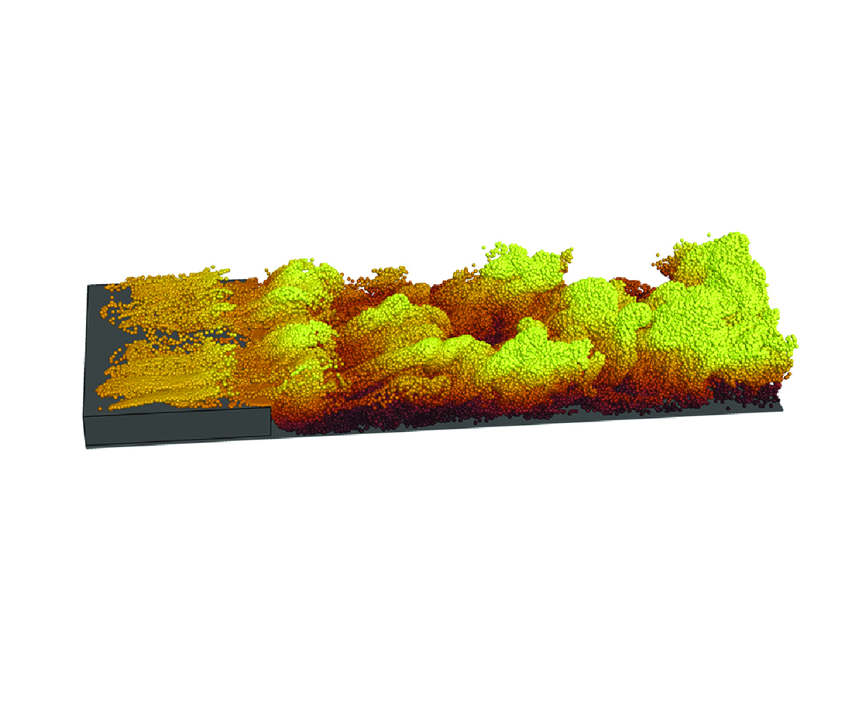
, with the dyes being uniformly distributed along the spanwise direction. Their spatial distributions, shown in figure 14, reveal that significant amounts of dye migrate to the upper side of the cylinder at
 $G/D=0.1$
(in figure 14
 $a$
). In contrast, for
 $G/D=0.3$
and
 $0.9$
, no dye is present above the cylinder (in figures 14
 $b$
and 14
 $c$
), indicating that at
 $G/D=0.1$
, downstream fluid is transported to the upper side of the cylinder due to wall recirculation. The distribution of virtual dyes in the near wake region shows the highest concentration for
 $G/D=0.1$
and the lowest for
 $G/D=0.9$
, consistent with the mean flow, where larger
 $G/D$
values result in weaker separation of the downstream wall boundary layer.
Results of tracking the evolution of the downstream wall recirculation at
 $L/D=5$
for different
 $G/D$
, revisited by virtual dye visualization:
 $(a)$
 $G/D=0.1$
;
 $(b)$
 $G/D=0.3$
;
 $(c)$
 $G/D=0.9$
. Colours represent wall-normal heights: red for higher heights and blue for lower heights.

3.2.1. The
 $G/D=0.1$
cases

The vortex distribution on the upper side of the cylinder at
 $L/D=5$
and
 $G/D=0.1$
differs significantly from the FIRC at the same
 $Re$
(Zhang et al. Reference Zhang, Kareem, Xu and Jiang2023; Li et al. Reference Li, Wang, Qiu, Zhou, Fu and Liu2024b
) (in figure 4), necessitating a detailed examination of the vortex dynamics, particularly the formation of the ULE vortex. The evolution of the vortex dynamics is shown in figure 15
 $(a,b)$
, with the instantaneous pressure distribution at
 $z/D=\pi$
in figure 15
 $(c,d)$
. At
 $t=t_0$
, a merged UKH vortex forms near the UTE (in figure 15
 $a$
), creating a low-pressure region and inducing a reverse flow beneath it, as seen in figure 15
 $(c)$
. Meanwhile, the UKH vortex undergoes 3-D instability and evolving into the ULE vortex. This reverse flow, encountering an adverse pressure gradient (in the inset of figure 15
 $c$
), causes the separation of the upper boundary layer, forming an anticlockwise-rotating SV on the upper side of the cylinder (USV), marked by the magenta arrow in figure 15
 $(a)$
. This USV is absent in the FIRC (Zhang et al. Reference Zhang, Kareem, Xu and Jiang2023; Li et al. Reference Li, Wang, Qiu, Zhou, Fu and Liu2024b
). The upstream motion generated by the downstream wall recirculation enhances the local reverse flow, which is a key factor contributing to the generation of the USV. At
 $t=t_0 + 12 \Delta t$
(in figures 15
 $b$
and 15
 $d$
), the ULE vortex detaches from the cylinder, displaying strong 3-D features and interacting with the wall recirculation. While the initial USV disappears, a new one forms due to the induction of the newly generated UKH vortex. The wall recirculation induced by the new UKH vortex passes over the UTE (in figure 15
 $b$
). This interaction directly contributes to the integration of the ULE recirculation and the downstream wall recirculation in the mean field (in figure 7
 $a$
) and prevents the formation of UTE vortices in the current flow. To confirm this phenomenon, 3-D FTLEs are employed.
(a,b) The process of the LLE vortex developing from the UKH vortex at
 $L/D=5$
and
 $G/D=0.1$
. (c,d) The corresponding instantaneous distribution of the pressure with the superimposition of instantaneous streamlines at
 $z/D=\pi$
. Here (a,c)
 $t=t_0$
; (b,d)
 $t=t_0+12\Delta t$
, where
 $\Delta t=0.25D/U_0$
. The vortical structures are visualized by isosurfaces of
 $Q=0.1$
, coloured with the instantaneous spanwise vorticity
 $\omega _z$
. The magenta arrow in (a) and (b) marks the SV with positive
 $\omega _z$
on the upper side of the cylinder. The insets in
 $(c)$
are the close-up views.

The vortex evolution process revealed by LCSs presented in the slices at
 $G/D=0.1$
: (a,b) the ULE vortex for
 $L/D=5$
, (c,d) the UTE vortex for
 $L/D=10$
. Here
 $(b)$
and
 $(d)$
are delayed by
 $8\Delta t$
and
 $4\Delta t$
compared with
 $(a)$
and
 $(c)$
, respectively, where
 $\Delta t=0.25D/U_0$
.

As shown in figure 16
 $(a,b)$
, the UKH vortex evolves into the ULE vortices as it passes over the UTE, but no UTE vortex is formed during this process. This confirms that UTE vortices do not form for
 $L/D=5$
and
 $G/D=0.1$
. While the reverse uplift of the downstream wall recirculation is observed. The formation of UTE vortices at larger aspect ratios is also examined. For
 $L/D = 15$
, the flow characteristics are similar to those for
 $L/D = 10$
. Therefore, only the vortex dynamics near the UTE for
 $L/D = 10$
are shown in figure 16
 $(c,d)$
. At time
 $t=t_0$
(in figure 16
 $c$
), the ULE vortex forms a hairpin vortex near the UTE, while the UTE shear layer rolls up, initiating the formation of a UTE vortex. This formation is driven by the KH instability of the UTE shear layer, similar to backward-facing step flows (Ma & Schröder Reference Ma and Schröder2017; Li et al. Reference Li, Zhang, Liu, Wu and Gao2020; Ma et al. Reference Ma, Tang and Jiang2020). By
 $t=t_0+4\Delta t$
(in figure 16
 $d$
), the UTE vortex fragments due to interactions with the wall recirculation, and is entrained into the wake and dissipates. In contrast, the ULE vortex retains its hairpin vortex shape and continues to evolve downstream, becoming the dominant feature in the plate boundary layer.
3.2.2. The
$G/D=0.3$
cases

To examine the development of the UTE and LTE shear layers at
 $G/D=0.3$
, FTLEs are also used for visualization. The evolution for
 $L/D=5$
is illustrated in figure 17
 $(a,b)$
. At
 $t=t_0$
(in figure 17
 $a$
), the UTE shear layer rolls up, forming the UTE vortex. This process contrasts with the flow at
 $G/D=0.1$
for the same
 $L/D$
. Moreover, the UTE shear layer deflects downwards, contributing to the formation of an upper recirculation (in figure 8
 $a$
). As the flow progresses, the UTE vortex is entrained into the wake and disappears (in figure 17
 $b$
). Meanwhile, the LTE shear layer lifts but does not roll up, preventing the formation of the LTE vortex in this flow. The formation of the UTE vortex at
 $L/D=10$
is shown in figure 17
 $(c,d)$
. The flow at
 $L/D=15$
exhibits similar behaviour, so it is not presented here. At
 $t=t_0$
(in figure 17
 $c$
), the UTE shear layer rolls up, generating two UTE vortices simultaneously. This double-TE vortex formation has not been reported in previous studies on the flows around rectangular cylinders. The UTE shear layer forms via KH instability, similar to the flow at
 $L/D=10$
with
 $G/D=0.1$
, and does not deflect downstream, resulting in no upper recirculation behind the cylinder (in figures 8
 $c$
and 8
 $e$
). By
 $t=t_0+8\Delta t$
(in figure 17
 $d$
), the upstream UTE vortex interacts with the ULE vortex, and breaks up. While the downstream one successfully develops into hairpin vortices. Despite the lifting of the LTE shear layer, no LTE vortex forms. This contrasts with the FNCC at
 $G/D=0.3$
(Li et al. Reference Li, Wang, Qiu, Wu, Zhou, Fu and Liu2022a) and even at lower
 $G/D=0.25$
(He et al. Reference He, Wang, Pan, Feng, Gao and Rinoshika2017), where the lower wake vortex forms and sheds, producing alternating vortex shedding dynamics.
The evolution process of the UTE vortex revealed by LCSs presented in the slices at
 $G/D=0.3$
: (a,b)
 $L/D=5$
;
 $(c,d)$
 $L/D=10$
. Here
 $(b)$
and
 $(d)$
are delayed by
 $6\Delta t$
and
 $8\Delta t$
compared with
 $(a)$
and
 $(c)$
, respectively, where
 $\Delta t=0.25D/U_0$
.

Close-up view of the instantaneous SV near the TE (TSV) and the vortex with positive spanwise vorticity on the plate wall (WPV) at
 $G/D=0.3$
, visualized by isosurfaces of
 $Q=0.05$
and coloured with the instantaneous spanwise vorticity
 $\omega _z$
, along with the slices showing the contours of instantaneous pressure with the superimposition of streamlines at
 $z/D=0$
:
 $(a)$
 $L/D=5$
;
 $(b)$
 $L/D=10$
. The azure rotation arrow represents local clockwise motion; the red rotation arrow represents local anticlockwise motion.

As shown in figure 8, multiple recirculations are observed downstream of the cylinder. The corresponding instantaneous vortex dynamics is investigated using the clustering method (Jiménez et al. Reference Jiménez, Del, Juan and Flores2004; Dong et al. Reference Dong, Huang, Yuan and Lozano-Durán2020; Wang et al. Reference Wang, Pan, Wang and Gao2022a
,Reference Wang, Pan and Wang
b
), previously effective in identifying secondary and tertiary vortices in the FNCC (Li et al. Reference Li, Wang, Qiu, Wu, Zhou, Fu and Liu2022a
). Here, the criteria for identifying significant vortex structures through clustering methods are defined by
 $Q \gt 0.05$
, with distinct characteristic structures differentiated by the positive or negative value of the spanwise vorticity
 $\omega _z$
. The extracted structures are shown in figure 18. Since the flow at
 $L/D=15$
is similar to that at
 $L/D=10$
(in figure 8), only the instantaneous structures for
 $L/D=10$
are discussed. As illustrated in figure 18, the vortex structure distributions for
 $L/D = 5$
and
 $L/D = 10$
display notable similarities. Secondary vortices with negative
 $\omega _z$
emerge downstream of the LTE shear layer. These vortices, positioned near the TE, are referred to as TSV. Immediately downstream, on the wall, vortex structures characterized by positive
 $\omega _z$
are observed, and are designated as WPV. This vortex distribution pattern closely resembles that observed in the FNCC at the same
 $G/D$
(Li et al. Reference Li, Wang, Qiu, Wu, Zhou, Fu and Liu2022a
), although the in the current flows, especially the secondary vortices, are less pronounced compared with those in the FNCC.
As shown in the inset of figure 18, in both two cases, the TSV originates from the plate boundary layer, driven by an adverse pressure gradient, as depicted by the smaller clockwise motion arrow near the plate wall. When the gap flow interacts with the downstream wall recirculation (the larger clockwise motion arrow), the WPVs forms. However, the dominant sources for WPV formation differ significantly with varying
 $L/D$
values. For
 $L/D=5$
(in the inset of figure 18
 $a$
), the wall recirculation is more pronounced, competing effectively with the gap flow, which causes a significant upward deflection of the gap flow. Near the wall, the WPV (the anticlockwise motion arrow) forms as the wall recirculation encounters the TSV. The intense wall recirculation brings two clockwise recirculations into close proximity – the wall recirculation itself and the one induced by the TSV. This proximity causes the wall recirculation to absorb the TSV-induced recirculation within the mean field, as illustrated in figure 8
 $(a)$
. Consequently, aside from the wall recirculation, only anticlockwise recirculation corresponding to the WPV is observed in the mean field. When
 $L/D=10$
(in the inset of figure 18
 $b$
), the wall recirculation diminishes, and the gap flow extends farther downstream following the formation of the TSV. Upon encountering the wall recirculation, the gap flow lifts upwards, creating a local adverse flow that leads to WPV formation. Thus, the WPV primarily originates from the gap flow, differing from the scenario at
 $L/D=5$
. Meanwhile, the wall recirculation and TSV are effectively blocked by the WPV, resulting in their independent existence in the mean field, as shown in figure 8
 $(b)$
. A comparison between the FNCC and FNRC reveals that: in the FNCC, vortices with positive
 $\omega _z$
are induced by secondary vortices; while in the FNRC, they result from the competition between the gap flow and wall recirculation. The dominant source is influenced by
 $L/D$
, which explains why these vortices (WPVs) are not named as TV in this study.
3.2.3. The
$G/D=0.9$
cases

For
 $L/D=5$
and
 $G/D=0.9$
, the formation of the TE vortex is examined in figure 19. At
 $t=t_0$
(in figure 19
 $a$
), the LTE sheds from the LTE shear layer, while the UTE shear layer rolls up. By
 $t=t_0+9\Delta t$
(in figure 19
 $b$
), the LTE vortex has shed off and evolved into wake. The UTE shear layer deflects downward, strengthening the UTE vortex. Then, the alternating shedding of upper and lower trailing vortices occurs, differing from the dynamics at
 $G/D=0.1$
and
 $0.3$
. Moreover, figure 19
 $(b)$
shows the LLE vortex and TSV, with their formation depicted in figure 20.
The evolution process of the UTE vortex revealed by LCSs presented in the slices for
 $L/D=5$
and
 $G/D=0.9$
:
 $(a)$
 $t=t_0$
;
 $(b)$
 $t=t_0+9\Delta t$
, where
 $\Delta t=0.25D/U_0$
.

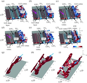
The vortex dynamics in the gap at
 $L/D=5$
and
 $G/D=0.9$
:
 $(a)$
 $t=t_0$
;
 $(b)$
 $t=t_0+5\Delta t$
;
 $(c)$
 $t=t_0+10\Delta t$
;
 $(d)$
 $t=t_0+15\Delta t$
;
 $(e)$
 $t=t_0+20\Delta t$
;
 $(f)$
 $t=t_0+25\Delta t$
, where
 $\Delta t=0.25D/U_0$
. Here
 $(g)$
,
 $(h)$
and
 $(i)$
are partial structures extracted from
 $(a)$
,
 $(b)$
and
 $(c)$
, respectively. The vortical structures are visualized by isosurfaces of
 $Q=0.1$
, coloured with the instantaneous spanwise vorticity
 $\omega _z$
. The magenta arrow marks the SV with negative
 $\omega _z$
on the lower side of the cylinder. The azure arrow marks TV
 $_1$
.

As shown in figure 20
 $(a)$
, at time
 $t=t_0$
, the LLE shear layer rolls up, forming the leading secondary vortex (LSV
 $_3$
) from the plate wall. Notably, the LSV forms before the LLE vortex. The LSV
 $_3$
undergoes instability, causing plate boundary layer separation and forming the weak TV
 $_2$
. The LLE vortex advances to
 $x/D \approx 4$
, where LSV
 $_2$
forms, while LSV
 $_1$
is located near the TE, with LSV
 $_2$
being smaller than LSV
 $_1$
. At
 $t=t_0 + 5\Delta t$
(in figure 20
 $b$
), the LE shear layer rolls farther, creating a SV with negative
 $\omega _z$
, which quickly dissipates downstream. Meanwhile, the enhanced TV
 $_2$
stabilizes LSV
 $_3$
, and the spanwise instability of the LLE vortex suppresses the growth of LSV
 $_2$
. By
 $t=t_0+10\Delta t$
(in figure 20
 $c$
), a new LLE vortex sheds. While the established one is transitioning into the LTE vortex. This transition does not occur in the FIRC (Cimarelli et al. Reference Cimarelli, Leonforte and Angeli2018b
, Reference Cimarelli, Leonforte, Angelis, Crivellini and Angeli2019a
; Chiarini & Quadrio Reference Chiarini and Quadrio2021; Chiarini et al. Reference Chiarini, Quadrio and Auteri2021, Reference Chiarini, Gatti, Cimarelli and Quadrio2022a
; Zhang et al. Reference Zhang, Kareem, Xu and Jiang2023; Cimarelli et al. Reference Cimarelli, Corsini and Stalio2024; Li et al. Reference Li, Wang, Qiu, Zhou, Fu and Liu2024b
). The LSV
 $_1$
convects downstream while LSV
 $_2$
fragments. At
 $t=t_0+15\Delta t$
(in figure 20
 $d$
), a weaker SV (LSV
 $_4$
) forms, indicating that each LLE vortex can induce two secondary vortices in one shedding cycle. The LTE vortex interacts with LSV
 $_1$
, and TV
 $_2$
flattens and merges into the LTE vortex. At
 $t=t_0+20\Delta t$
(in figure 20
 $e$
), the LTE vortex lifts, causing LSV
 $_1$
to rise. The LSV
 $_2$
, previously fragmented, is enhanced by the LTE vortex. At
 $t=t_0+25\Delta t$
(in figure 20
 $f$
), the LTE vortex sheds off, and LSV
 $_1$
deforms and rises. The LSV
 $_2$
is enhanced but no new SV forms near the LTE. The separation of the wall boundary layer near the LTE results from the established weak LSV. The TV
 $_2$
does not shed with the LTE vortex; instead, it forms a pseudo-TE vortex, with its shedding corresponding to the evolution of TV
 $_1$
(in figure 20
 $a-c$
), which is extracted through the clustering method and shown in figure 20
 $(g-i)$
. After shedding, TV
 $_2$
does not rise like the LTE vortex but convects downstream. Double-secondary vortices, similar to those observed in multielement airfoils (Wang, Wang & Kim Reference Wang, Wang and Kim2019; Wang & Wang Reference Wang and Wang2021b
) and simplified circular-cylinder/airfoil configurations (Wang, Wu & Wang Reference Wang, Wu and Wang2023), also appear in the FNCC boundary layer at
 $G/D=1.0$
and
 $1.333$
(Wang et al. Reference Wang, He and Wang2024). However, the secondary vortices in this study are smaller and weaker, distinguishing them from previous double-SV configurations.
The vortex dynamics in the gap at
 $L/D=15$
and
 $G/D=0.9$
:
 $(a)$
 $t=t_0$
;
 $(b)$
 $t=t_0+7\Delta t$
; where
 $\Delta t=0.25D/U_0$
. The vortical structures are visualized by isosurfaces of
 $Q=0.1$
, coloured with the instantaneous spanwise vorticity
 $\omega _z$
.

The vortex dynamics at
 $L/D=10$
will be discussed in
 $\S$
3.3.1, influenced by two distinct frequencies. For
 $L/D=15$
, as shown in figure 21, vortex formation is similar to
 $L/D=5$
, but no double-secondary vortices form from the plate boundary layer. The LKH vortex rapidly evolves into the LLE vortex in the form of a streamwise vortex pair, as shown in figure 21
 $(a)$
. Figure 21
 $(b)$
indicates the LSV exhibits spanwise instability, reversely inducing lower boundary layer separation and forming a TV, as at
 $L/D=5$
. Unlike at
 $L/D=5$
, the LSV does not return to a two-dimensional structure, instead stretching into hairpin-like vortices. The TV strengthens under the influence of TSV but breaks up due to mean shear. Two adjacent TV groups merge near the LTE, forming an LTE vortex, which induces a TSV from the plate boundary layer.
3.3. Frequency characteristics
In the FIRC at medium
 $Re$
, the LE and TE vortices shed at the same frequency for a fixed
 $L/D$
, exhibiting frequency locking. Multiple KH vortices merge to form a cohesive LE vortex. These dynamics can be reflected in the PSD (Wang & Wang Reference Wang and Wang2021a
; Tian et al. Reference Tian, Xu, Duan and Wang2023; Duan & Wang Reference Duan and Wang2024; Li et al. Reference Li, Wang, Qiu, Zhou, Fu and Liu2024b
; Zhang et al. Reference Zhang, Li, Wang, Qiu, Fu and Liu2024; Zhou et al. Reference Zhou, Qiu, Li, Wang, Zhou and Liu2024). The influence of near-wall effects on frequency characteristics and vortex dynamics will be examined in the context of the FIRC.
Local PSDs of streamwise velocity fluctuation at different spatial locations for
 $G/D=0.1$
and
 $G/D=0.3$
: (a,c,e)
 $G/D=0.1$
; (b,d,f)
 $G/D=0.3$
; (a,b)
 $L/D=5$
; (c,d)
 $L/D=10$
; (e,f)
 $L/D=15$
. The PSDs are calculated at azure points in figure 13(a,b) and remain marked by the same numbers. The amplitudes of PSDs for azure point 2
 $-$
7 are amplified step-by-step by
 $10^{3}$
along the serial number. Here
 $St_0$
,
 $St_{01}$
,
 $St_{02}$
and
 $St_{03}$
denote the shedding frequencies of the LE or TE vortex;
 $St_{0*}$
is the pseudoshedding frequency;
 $St_{\textit {KH}}$
is KH fluctuation frequency. The orange circle marks
 $0.5St_0$
, while the lime green circle marks
 $1.5St_0$
. The dashed lines define the frequency bands with a bandwidth of
 $0.02$
, related to the typical frequencies.

3.3.1. Flow processes with typical frequencies
The PSDs are calculated at the azure points in figure 13, and remain marked by the same numbers. The velocity fluctuations at this location are typically the highest locally, particularly at points 1–3, which are distributed along the shear layer. The characteristic peaks detected at nearly all monitoring points within a flow can be used to identify the corresponding characteristic frequency of the flow. Figure 22
 $(a,c,e)$
, show the PSDs at various spatial positions for different
 $L/D$
ratios at
 $G/D=0.1$
. For
 $L/D = 5$
, as illustrated in figure 22
 $(a)$
, a prominent fluctuation signal is observed from the LE shear layer extending to the downstream wall recirculation, which corresponds to the fundamental frequency
 $St_0$
and is characteristic of the LE vortex dynamics. Probes 1–3 show
 $0.5St_0$
(marked by the red circle),
 $1.5St_0$
(marked by the blue circle) and
 $St_{\textit {KH}}$
(
 $St_{\textit {KH}}=2St_0$
), with the subharmonic
 $0.5St_0$
and fractional harmonic
 $1.5St_0$
resulting from nonlinear interactions. The
 $St_{\textit {KH}}$
weakens downstream and represents the fluctuation frequency of KH instability within the ULE shear layer. The relation
 $St_{\textit {KH}}=2St_0$
indicates that every two UKH vortices merge to form a single ULE vortex during one shedding cycle. In contrast, in the FIRC at
 $L/D=5$
, every three KH vortices merge into one LE vortex (Zhang et al. Reference Zhang, Kareem, Xu and Jiang2023; Li et al. Reference Li, Wang, Qiu, Zhou, Fu and Liu2024b
). The merging process of UKH vortices for
 $G/D=0.1$
and
 $L/D=5$
is shown in figure 23. Instantaneous vortices visualized with isosurfaces of
 $Q=0.5$
reveal that adjacent UKH vortices shed from the ULE shear layer, merging downstream, as shown in figure 23
 $(a-d)$
. After merging, the vortex becomes 3-D and evolves into the ULE vortex. Notably, the UKH vortices merge before undergoing 3-D instability here, whereas in the FIRC, instability occurs first (Zhang et al. Reference Zhang, Kareem, Xu and Jiang2023). The near-wall effect influences both the number and sequence of merging and instability. Furthermore, figure 22
 $(a)$
shows consistent characteristic frequencies across all probes, including in the downstream recirculation, indicating that the frequency-locking feature persists in the FNRC with
 $L/D=5$
and
 $G/D=0.1$
.
For
 $L/D=10$
and
 $G/D=0.1$
, figure 22
 $(c)$
shows the fundamental frequency
 $St_0$
in the PSDs for all probes. Additionally, a new frequency
 $St_{0*}$
, similar to
 $St_0$
, is detected in probes 1 and 2 within the ULE shear layer but weakens and disappears downstream. This is interpreted as a pseudoshedding frequency, to be validated by DMD analysis in § 3.3.2. In probe 1, the dominant frequency with a wide bandwidth is
 $St_0$
, indicating that the ULE vortex primarily originates from a single UKH vortex. The evolution of the ULE vortex from the UKH vortex is shown in figure 24. Notably, adjacent UKH vortices do not merge but directly evolve into ULE vortices in the form of hairpin vortices. In contrast, in the FIRC with
 $L/D=10$
, every two KH vortices merge to form an LE vortex (Li et al. Reference Li, Wang, Qiu, Zhou, Fu and Liu2024b
). As
 $L/D$
increases to
 $15$
, figure 22
 $(d)$
shows two distinct shedding frequencies,
 $St_{01}$
and
 $St_{02}$
, due to mode competition, which will be discussed further in the DMD analysis in § 3.3.2. The evolution of the UKH vortex into the ULE vortex at
 $L/D=15$
is similar to
 $L/D=10$
. For
 $G/D=0.3$
, the PSDs for different
 $L/D$
ratios (in figure 22
 $b,d,f$
) are similar to those at
 $G/D=0.1$
, except at
 $L/D=15$
, where three-mode competition arises.
The process of the UKH vortex merging at
 $G/D=0.1$
and
 $L/D=5$
:
 $(a)$
 $t=t_0$
;
 $(b)$
 $t=t_0+2\Delta t$
;
 $(c)$
 $t=t_0+4\Delta t$
;
 $(d)$
 $t=t_0+6\Delta t$
, where
 $\Delta t=0.25D/U_0$
. The vortical structures are visualized by isosurfaces of
 $Q=0.5$
, coloured with the instantaneous streamwise velocity
 $u/U_0$
. The black arrow marks the UKH vortex.

The process of the UKH vortex evolving into the ULE vortex at
 $G/D=0.1$
and
 $L/D=10$
:
 $(a)$
 $t=t_0$
;
 $(b)$
 $t=t_0+10\Delta t$
;
 $(c)$
 $t=t_0+20\Delta t$
, where
 $\Delta t=0.25D/U_0$
. The vortical structures are visualized by isosurfaces of
 $Q=0.5$
, coloured with the instantaneous streamwise velocity
 $u/U_0$
. The arrow marks the UKH vortex.

Local PSDs of streamwise velocity fluctuation at different spatial locations for
 $G/D=0.9$
: (a,b)
 $L/D=5$
; (c,d)
 $L/D=10$
; (e,f)
 $L/D=15$
. The PSDs are calculated at azure points in figure 13
 $(c)$
and remain marked by the same numbers. The amplitudes of PSDs for azure point 2
 $-$
5 and 7
 $-$
9 are amplified step-by-step by
 $10^{3}$
along the serial number. Here
 $St_0$
,
 $St_{01}$
and
 $St_{02}$
denote the shedding frequencies of the LE or TE vortex;
 $St_{0*}$
is the pseudoshedding frequency. The dashed lines define the frequency bands with a bandwidth of
 $0.02$
, related to the typical frequencies.

The local PSDs for
 $G/D=0.9$
are presented in figure 25. For
 $L/D=5$
, figures 25
 $(a)$
and 25
 $(b)$
show the fundamental frequency
 $St_0$
is present in all probes, confirming frequency locking and that the characteristic frequency of SV coincides with
 $St_0$
. A high-frequency band at four times
 $St_0$
suggests four UKH vortices shed from the ULE shear layer in one LE/TE shedding cycle. The evolution of this process is illustrated in figure 26. At
 $t=t_0$
(figure 26
 $a$
), UKH
 $_{1}$
and UKH
 $_{2}$
form, while the LTE shear layer rolls up to create an LTE vortex. The UKH
 $_{1}$
evolves into hairpin vortices, while UKH
 $_{2}$
strengthens the LTE vortex (in figure 26
 $b$
and 26
 $c$
). By
 $t=t_0+15\Delta t$
(in figure 26
 $d$
), UKH
 $_{3}$
forms and, along with UKH
 $_{2}$
, merges to form the ULE vortex (in figure 26
 $e$
), with the LTE vortex shedding off. As shown in figure 26
 $(f)$
, the merged vortex separates, while a new UKH vortex (UKH
 $_{4}$
) begins to form. Notably, although four UKH vortices are generated, not all participate in merging. The PSDs from probes 7 and 8 show harmonics of
 $St_0$
, attributed to downstream convection of the TV and the enhancement of the weak LSV, resembling the harmonics seen in double-secondary vortices in the FNCC (Wang et al. Reference Wang, He and Wang2024).
The process of the UKH vortex evolving into the ULE vortex at
 $G/D=0.9$
and
 $L/D=5$
:
 $(a)$
 $t=t_0$
;
 $(b)$
 $t=t_0+5\Delta t$
;
 $(c)$
 $t=t_0+10\Delta t$
;
 $(d)$
 $t=t_0+15\Delta t$
;
 $(e)$
 $t=t_0+20\Delta t$
;
 $(f)$
 $t=t_0+25\Delta t$
, where
 $\Delta t=0.25D/U_0$
. The vortical structures are visualized by isosurfaces of
 $Q=0.5$
, coloured with the instantaneous streamwise velocity
 $u/U_0$
. The magenta arrow marks the LTE vortex.

The PSDs for
 $L/D=10$
and
 $G/D=0.9$
are illustrated in figures 25
 $(c)$
and 25
 $(d)$
. Two dominant frequencies,
 $St_{01}$
and
 $St_{02}$
, are observed. At probe 1, both frequencies are distinct, but at probes 2 and 3,
 $St_{02}$
becomes dominant, while
 $St_{01}$
weakens. The wide bandwidth at probes 1 and 2 indicates that a single ULE vortex evolves from a UKH vortex, with shedding frequency
 $St_{02}$
. At probe 4, downstream,
 $St_{01}$
reappears, signalling double-mode competition as the flow becomes more complex and wall boundary layer characteristics emerge (in figure 6
 $b$
). At probe 5, near the UTE vortex shedding location, a reduction in the peaks of both frequencies occurs, with
 $St_{01}$
still detectable and
 $St_{02}$
disappearing, indicating the UTE vortex shedding frequency is
 $St_{01}$
. This marks a shift in the characteristic frequency from
 $St_{02}$
to
 $St_{01}$
on the upper side of the cylinder. At probe 6, within the LLE shear layer, both
 $St_{01}$
and
 $St_{02}$
remain, but no wide bandwidth is observed, suggesting bimodal competition in LLE vortex formation. At probes 8 and 9, associated with the LTE vortex shedding and TSV formation, the frequency is
 $St_{01}$
, with
 $St_{02}$
diminishing. This shows that frequency locking is suppressed in the flow at
 $G/D=0.9$
and
 $L/D=10$
.
The presence of two dominant frequencies warrants investigation into their effects on vortex dynamics. The signals for
 $St_{01}$
and
 $St_{02}$
are extracted via Fourier mode decomposition (Basley et al. Reference Basley, Pastur, Lusseyran, Faure and Delprat2011; Ma et al. Reference Ma, Feng, Pan, Gao and Wang2015; Wang et al. Reference Wang, Feng, Wang and Li2018; Wang & Wang Reference Wang and Wang2021a
,Reference Wang and Wang
b
; Li et al. Reference Li, Wang, Qiu, Zhou, Fu and Liu2024b
) from probe 7 at
 $z/D=\pi$
, as shown in figure 13(
 $c$
i). The results, presented in figure 27, show strong competition between the two frequencies: when
 $St_{01}$
fluctuates strongly,
 $St_{02}$
weakens and vice versa. Specifically, around time
 $t=t_a$
, the fluctuation is dominated by
 $St_{01}$
, while
 $St_{02}$
is weak; the reverse occurs at
 $t=t_b$
. The vortex dynamics for
 $L/D=10$
and
 $G/D=0.9$
in figure 28 resemble those at
 $L/D=15$
and
 $G/D=0.9$
(in figure 21), but the SV evolution differs between the two frequencies. When
 $St_{01}$
is dominant, hairpin-like vortices form from the LSV (in figures 28
 $a$
and 28
 $b$
), as seen at
 $L/D=15$
. In contrast, when
 $St_{02}$
dominates, no hairpin vortices form, and only spanwise vortices are present (in figures 28
 $c$
and 28
 $d$
). Additionally, with
 $St_{01}$
, the LTE vortex sheds before the TV reaches the LTE, whereas for
 $St_{02}$
, the LTE vortex has not yet shed at that point. This phase difference results from the competition between the two frequencies but does not affect the characteristic frequencies of the LTE vortex and TSV, as shown in figure 25
 $(d)$
at probes 8 and 9.
The time signals of streamwise velocity fluctuation for
 $St_{01}$
and
 $St_{02}$
at
 $L/D=10$
and
 $G/D=0.9$
. The azure and orange curves are the signals of the Fourier mode decomposition mode for
 $St_{01}$
and
 $St_{02}$
, respectively, which are extracted from the probe 7 (presented in figure 13
c i) in the plane
 $z/D=\pi$
. Here
 $t_a$
and
 $t_b$
mark the typical instances for the strong fluctuations of
 $St_{01}$
and
 $St_{02}$
, respectively.

The instantaneous vortical structures in the gap for
 $L/D=10$
and
 $G/D=0.9$
:
 $(a)$
 $t=t_a-8\Delta t$
;
 $(b)$
 $t=t_a$
;
 $(c)$
 $t=t_b-8\Delta t$
;
 $(d)$
 $t=t_b$
, where
 $\Delta t=0.25D/U_0$
. The vortical structures are visualized by isosurfaces of
 $Q=0.1$
, coloured with the instantaneous spanwise vorticity
 $\omega _z$
.

The process of the UKH vortex evolving into the ULE vortex at
 $L/D=15$
and
 $G/D=0.9$
:
 $(a)$
 $t=t_0$
;
 $(b)$
 $t=t_0+5\Delta t$
;
 $(c)$
 $t=t_0+10\Delta t$
;
 $(d)$
 $t=t_0+15\Delta t$
, where
 $\Delta t=0.25D/U_0$
. The vortical structures are visualized by isosurfaces of
 $Q=0.5$
, coloured with the instantaneous streamwise velocity
 $u/U_0$
. The magenta arrow marks the UKH vortex, and the ellipse marks the ULE vortex in the form of the hairpin vortex cluster.

The process of LLE vortex shedding being suppressed at
 $L/D=15$
and
 $G/D=0.9$
:
 $(a)$
 $t=t_0$
;
 $(b)$
 $t=t_0+2\Delta t$
;
 $(c)$
 $t=t_0+4\Delta t$
;
 $(d)$
 $t=t_0+6\Delta t$
;
 $(e)$
 $t=t_0+8\Delta t$
;
 $(f)$
 $t=t_0+10\Delta t$
, where
 $\Delta t=0.25D/U_0$
. The vortical structures are visualized by isosurfaces of
 $Q=0.1$
, coloured with the instantaneous spanwise vorticity
 $\omega _z$
. The black arrow marks the LSV, the magenta arrow marks the LLE shear layer.

As
 $L/D$
increases to 15, the PSDs in figures 25
 $(e)$
and 25
 $(f)$
show a single fundamental frequency,
 $St_0$
, across all probes, indicating frequency locking despite the presence of a pseudofrequency related to vortex shedding. In the PSD at probe 1 within the ULE shear layer, the dominant high-frequency bandwidth is
 $2St_0$
, suggesting that two UKH vortices merge to form one ULE vortex. This is illustrated in figure 29, where two adjacent UKH vortices shed from the ULE shear layer (in figure 29
 $a$
), interact with the ULE recirculation (in figure 29
 $b$
), and evolve into 3-D vortices (in figure 29
 $c$
). They then merge to form a ULE vortex, a hairpin vortex cluster (in figure 29
 $d$
). This process, where UKH vortices first undergo 3-D instability before merging, contrasts with the behaviour at
 $L/D=5$
and
 $G/D=0.1$
(in figure 23). Additionally, figure 25
 $(f)$
shows a wide bandwidth around
 $2St_0$
at probe 6, but the merging of LKH vortices into an LLE vortex does not occur here. This suppression occurs because the enhanced LSV inhibits the formation of KH vortices when the LLE shear layer undergoes the second KH instability. As a result, only the first KH instability contributes to the formation of KH vortices within a single shedding cycle. As shown in figure 30, the LKH vortex quickly evolves into the LLE vortex and experiences local instability figure 30(
 $b{-}d$
). However, as the LSV strengthens, it suppresses the instability of the LLE shear layer figure 30(
 $e{-}f$
), preventing the formation of additional LKH vortices during the same shedding cycle.
3.3.2. Dynamic mode decomposition analysis
Isosurfaces of the real part of the DMD mode for the streamwise component at
 $G/D=0.1$
:
 $(a)$
 $St_0$
mode for
 $L/D=5$
;
 $(b)$
 $St_0$
mode for
 $L/D=10$
;
 $(c)$
 $St_{01}$
mode for
 $L/D=15$
;
 $(d)$
 $St_{02}$
mode for
 $L/D=15$
. (i) The values are
 $\pm 0.0001$
; (ii) the values are
 $\pm 0.0005$
. The red parts are positive and the blue parts are negative. The arrows mark the periodic topological structures.

Isosurfaces of the real part of the DMD mode for the streamwise component at
 $G/D=0.3$
:
 $(a)$
 $St_0$
mode for
 $L/D=5$
;
 $(b)$
 $St_0$
mode for
 $L/D=10$
;
 $(c)$
 $St_{01}$
mode for
 $L/D=15$
;
 $(d)$
 $St_{02}$
mode for
 $L/D=15$
;
 $(e)$
 $St_{03}$
mode for
 $L/D=15$
. (i) The values are
 $\pm 0.0001$
; (ii) the values are
 $\pm 0.0005$
. The red parts are positive and the blue parts are negative. The arrows mark the periodic topological structures.

To further investigate the dynamic characteristics of vortex shedding in the current FNRC, the DMD method is employed, akin to the analyses conducted on the FNCC (Li et al. Reference Li, Wang, Qiu, Wu, Zhou, Fu and Liu2022a ) and FIRC (Zhang et al. Reference Zhang, Kareem, Xu and Jiang2023; Li et al. Reference Li, Wang, Qiu, Zhou, Fu and Liu2024 b). This approach aims to explore the spatial characteristics of vortex shedding frequencies across all flows examined. Particular attention will be directed towards flows exhibiting multiple characteristic shedding frequencies, with the DMD method utilized to identify the dominant frequency for each flow.
Figure 31 illustrates the DMD analysis of ULE/UTE vortex shedding for flows with
 $G/D=0.1$
. The displayed topology represents the streamwise component of the DMD mode, with the structures in figures 31(
 $a$
i) to 31(
 $d$
i) showing similarities across different flows. These topological structures exhibit a regular alternating pattern in the streamwise direction, confirming the periodic nature of the flow and the presence of frequency locking. At
 $L/D=15$
, both
 $St_{01}$
and
 $St_{02}$
modes show periodicity, indicating competition between the two modes. However, the
 $St_{02}$
mode is more pronounced and persists farther downstream (in figure 31
 $d$
i). To identify the dominant shedding mode, the isosurface values of the DMD mode are increased, showing stronger fluctuations in figures 31(
 $a$
ii) to 31(
 $d$
ii). The DMD topological structures for
 $St_0$
at
 $L/D=5$
and
 $L/D=10$
and
 $St_{02}$
at
 $L/D=15$
maintain great coherence, reflecting flow periodicity. However, as the flow enters the plate boundary layer state, the stronger fluctuations dissipate, and the coherence of the
 $St_{01}$
mode at
 $L/D=15$
nearly disappears. Thus, the dominant frequency for the flow at
 $L/D=15$
and
 $G/D=0.1$
is
 $St_{02}$
.
For
 $G/D=0.3$
, the DMD vortex shedding topologies are presented in figure 32. The topological structures in figures 32(
 $a$
i) to 32(
 $e$
i) exhibit strong periodicity, similar to those at
 $G/D=0.1$
, until the flow transitions into the boundary layer state. The
 $St_{0*}$
mode at
 $L/D=10$
, representing the pseudoshedding frequency, is shown in figure 34
 $(a)$
with identical isosurface values. This mode lacks spatial coherence, explaining its inability to capture flow periodicity and justifying its designation as a pseudoshedding frequency. The topologies for stronger fluctuations, shown in figures 32(
 $a$
ii) to 32(
 $e$
ii), reveal that the
 $St_0$
modes at
 $L/D=5$
and
 $L/D=10$
maintain great periodicity. However, at
 $L/D=15$
, only the
 $St_{02}$
mode exhibits coherence, indicating it as the dominant mode despite the presence of three competing shedding frequencies. The
 $St_{0*}$
mode at
 $L/D=10$
continues to lack spatial coherence, as shown in figure 34
 $(b)$
.
Isosurfaces of the real part of the DMD mode for the streamwise component at
 $G/D=0.9$
:
 $(a)$
 $St_0$
mode for
 $L/D=5$
;
 $(b)$
 $St_{01}$
mode for
 $L/D=10$
;
 $(c)$
 $St_{02}$
mode for
 $L/D=10$
;
 $(d)$
 $St_0$
mode for
 $L/D=15$
. (i) The values are
 $\pm 0.0001$
; (ii) the values are
 $\pm 0.0005$
. The red parts are positive and the blue parts are negative. The arrows mark the periodic topological structures.

Isosurfaces of the real part of the DMD mode for the streamwise component: (a,b)
 $St_{0*}$
mode for
 $L/D=10$
and
 $G/D=0.3$
;
 $(c)$
 $St_{01}$
mode for
 $L/D=10$
and
 $G/D=0.9$
;
 $(d)$
 $St_{02}$
mode for
 $L/D=10$
and
 $G/D=0.9$
.
 $(a)$
The values are
 $\pm 0.0001$
; (b,c,d) the values are
 $\pm 0.0005$
. The red parts are positive and the blue parts are negative. The arrows mark the periodic topological structures corresponding to streamwise vortices in the gap.

As
 $G/D$
increases to
 $0.9$
, all topological structures capture the periodicity of vortex shedding, similar to the smaller gap ratios, as shown in figures 33(
 $a$
i) to 33(
 $d$
i). These structures confirm the instability of the LLE shear layer, leading to vortex formation. At
 $L/D=5$
, the mode exhibits a Kármán vortex street pattern, indicating a reduced near-wall effect. At
 $L/D=10$
, the
 $St_{02}$
mode shows greater coherence than
 $St_{01}$
, with topologies capturing the periodicity of the LE and TE vortices. However, the
 $St_{01}$
mode captures the periodicity of UTE and LTE vortices, while
 $St_{02}$
reflects the ULE vortex but loses coherence near the TE. Thus, the
 $St_{01}$
mode governs UTE and LTE vortices shedding, while
 $St_{02}$
regulates ULE vortices shedding. This agrees with the PSDs in figures 25
 $(c)$
and 25
 $(d)$
, confirming the suppression of frequency locking at
 $L/D=10$
and
 $G/D=0.9$
. Figures 34
 $(c)$
and 34
 $(d)$
show the DMD topologies of the stronger fluctuations for
 $St_{01}$
and
 $St_{02}$
modes. Near the LTE, the
 $St_{01}$
mode shows elongated streamwise features from the LSV, while
 $St_{02}$
lacks these structures. These topologies correlate with the vortices in figures 28
 $(a)$
and 28
 $(b)$
, indicating competitive coexistence within the LLE shear layer, where
 $St_{01}$
promotes streamwise vortices and
 $St_{02}$
suppresses them.
3.4. Discussion
In the current FNRC, multiple vortex shedding modes compete, similar to the findings by Chiarini et al. (Reference Chiarini, Quadrio and Auteri2022c
) in the FIRC at
 $Re=400$
. They observed that TE vortex shedding is key to flow locking, while the LE shear layer remains active in instability. Both two flow configurations can be stable under certain conditions, but at
 $Re=1000$
, vortex shedding tends to be fixed (Li et al. Reference Li, Wang, Qiu, Zhou, Fu and Liu2024b
). In the present flows, the near-wall effect disrupts symmetry and the feedback loop, particularly affecting the instability position of the LE shear layer and the reattachment point along the cylinder sides. Consequently, these factors disturb the original flow patterns, including the fixed vortex shedding modes across different
 $L/D$
ratios, leading to the active LE shear layer that facilitates the emergence of multiple vortex shedding modes. Ultimately, this results in instances of mode competition. Chiarini et al. (Reference Chiarini, Quadrio and Auteri2022c
) noted that in the FIRC, flow frequency locks onto the LE vortices passing over the TE corners, selecting the configuration with the longest shedding period. Li et al. (Reference Li, Wang, Qiu, Zhou, Fu and Liu2024b
) found that at
 $Re=1000$
, the shedding pattern is contralateral at
 $L/D=10$
, differing from ipsilateral shedding at
 $L/D=5$
and
 $L/D=15$
. In this study, alternating TE vortex shedding occurs at
 $G/D=0.9$
. However, due to flow asymmetry across the cylinder, the contralateral shedding pattern cannot be sustained at
 $L/D=10$
. This disrupts the feedback loop, preventing the flow from locking onto the LE vortex frequency and selecting the longest shedding period, as seen in the FIRC. Instead, the TE vortex shedding mode at
 $L/D=10$
and
 $G/D=0.9$
has a shorter period.
Through DMD analysis, the dominant shedding frequencies for each flow are shown in figure 35. For comparison, vortex shedding frequencies from the FIRC at the same
 $Re$
are also included. The results show that the near-wall effect raises the vortex shedding frequency, promoting vortex shedding. At
 $L/D=10$
and
 $G/D=0.9$
, two dominant frequencies are observed due to suppressed frequency locking. The higher frequency of ULE vortex shedding is similar to the findings of Zhang et al. (Reference Zhang, Kareem, Xu and Jiang2023), who reported a higher frequency for LE vortices in the FIRC with a splitter plate, independent of the TE vortex. This is also observed in the present flow. When the LE and TE vortices are no longer locked to the same frequency, the ULE vortex frequency significantly exceeds that of the TE vortex. This higher frequency is also present in the shedding process of the LLE vortex. Focusing on the TE vortex shedding frequency across circular and rectangular cylinders, as
 $G/D$
increases from
 $0.1$
to
 $0.3$
, the wake vortex frequency rises significantly. However, as
 $G/D$
increases further to
 $0.9$
, the frequency decreases. This pattern is consistent across different
 $L/D$
values. In the FNCC, the shedding frequency increases as
 $G/D$
decreases from around
 $2$
to
 $0.5$
, then decreases further with smaller
 $G/D$
(Lin et al. Reference Lin, Lin, Hsieh and Dey2009; He et al. Reference He, Wang, Pan, Feng, Gao and Rinoshika2017; Li et al. Reference Li, Wang, Qiu, Wu, Zhou, Fu and Liu2022a
). According to Jiang et al. (Reference Jiang, Ju, Guo and Wang2024), the increase in
 $St(L)$
from
 $G/D=0.1$
to
 $0.3$
is due to the plate wall influence, while the decrease from
 $G/D=0.3$
to
 $0.9$
is linked to the upstream wall boundary layer development.
The Strouhal number based on the streamwise dimension of the rectangular cylinder
 $St(L)$
at different aspect ratios and gap ratios compared with the results for the FIRC from the studies of Nakamura et al. (Reference Nakamura, Ohya and Tsuruta1991), Zhang et al. (Reference Zhang, Kareem, Xu and Jiang2023) and Li et al. (2024b).

4. Conclusion
This study presents a novel investigation into the vortex dynamics of a FNRC using DNS, marking the first comprehensive exploration of these phenomena. By varying the aspect ratios (
 $L/D = 5$
,
 $10$
and
 $15$
) and gap ratios (
 $G/D = 0.1$
,
 $0.3$
and
 $0.9$
) while maintaining a fixed
 $Re$
of
 $Re = 1000$
, the study reveals the complex evolution of vortex structures, mean flow topology and frequency characteristics influenced by the near-wall effect. The results demonstrate that both
 $L/D$
and
 $G/D$
significantly affect vortex dynamics, leading to the emergence of novel vortex behaviours that are not observed in FIRC or FNCC.
The mean flow topology reveals that smaller gap ratios (
 $G/D = 0.1$
,
 $0.3$
) suppress the LLE recirculation, while larger gap ratios (
 $G/D = 0.9$
) promote the formation of a LLE shear layer. The wall-normal scale of the ULE recirculation is smaller than that observed in the FIRC for all flows and increases with
 $G/D$
, whereas the streamwise scale is larger due to the delayed reattachment. At
 $L/D = 5$
, the ULE recirculation nearly spans the entire upper side of the cylinder for all values of
 $G/D$
. Reattachment occurs first at
 $G/D = 0.3$
across all aspect ratios, although the shear intensity of the ULE shear layer decays more rapidly at
 $G/D = 0.9$
. As the cylinder moves farther from the wall, fluctuations gradually increase, reflecting the diminishing influence of the near-wall effect.
In terms of vortex dynamics, the complexity of the vortex distribution increases as
 $G/D$
increases. The UKH vortex formed by the ULE shear layer undergoes a transition into the ULE vortex for all cases. At smaller gap ratios, the merging of UKH vortices forms the ULE vortex before undergoing further instability, which contrasts with the dynamics observed in the FIRC. As
 $G/D$
increases, more intricate vortex shedding modes emerge, with frequency locking observed in most flows. However, this phenomenon is suppressed at
 $L/D = 10$
and
 $G/D = 0.9$
. The trend in shedding frequency follows a pattern similar to the FNCC: as
 $G/D$
increases from
 $0.1$
to
 $0.3$
, the shedding frequency increases, while a decrease occurs as
 $G/D$
rises from
 $0.3$
to
 $0.9$
. The primary vortex dynamic behaviours at different gap ratios are summarized as follows.
-
(i) G/D = 0.1. The formation of the LTE vortex is suppressed, and alternating vortex shedding is absent. At
$L/D = 5$
, the UTE vortex is absent, resulting in a direct connection between the ULE recirculation and the downstream wall recirculation. This forms a continuous recirculation, allowing fluid to flow from the downstream region back to the upper side of the cylinder. The ULE vortex at
$L/D = 5$
is formed by the merging of two UKH vortices, whereas at larger aspect ratios (
$L/D = 10$
and
$15$
), it results from a single UKH vortex. -
(ii) G/D = 0.3. Similar to
$G/D = 0.1$
, the formation of the LTE vortex is suppressed, though the dynamics differ from those in the FNCC at the same
$G/D=0.3$
. At larger
$L/D$
, a novel phenomenon occurs with the emergence of double-TE vortices. Two distinct generation mechanisms for the WPV are identified: for
$L/D = 5$
, strong wall recirculation leads to the formation of the WPV, which absorbs TSV-induced recirculation; at
$L/D = 10$
and
$15$
, the WPV is primarily generated by the gap flow, preventing the absorption of wall recirculation. The UKH vortices continue to merge to form ULE vortices, consistent with the behaviour observed at
$G/D = 0.1$
. -
(iii) G/D = 0.9. The LKH vortex (LLE vortex) forms, giving rise to the LSV from the wall, which in turn contributes to the formation of a TV from the lower boundary layer of the cylinder. At
$L/D = 5$
, the LLE vortex and TV evolve into the LTE vortex and pseudo-TE vortex, respectively. Double-secondary vortices form, consisting of one strong vortex that rises with the LTE vortex into the wake and a weaker vortex that strengthens during this process. A notable observation is that although four UKH vortices are generated, only two of them merge. As
$L/D$
increases, the SV signal becomes more pronounced, and the LLE vortex quickly evolves into a streamwise vortex pair, with the TV eventually transforming into the TE vortex. At
$L/D = 15$
, the LSV develops into hairpin-like vortices, while two UKH vortices merge to form a single ULE vortex, mirroring the behaviour observed in the FIRC. At
$L/D = 10$
, however, the development of the LSV is influenced by two competing shedding modes with different frequencies: the lower-frequency mode, which governs the TE vortex shedding, promotes the formation of streamwise vortices, while the higher-frequency mode, responsible for ULE vortex shedding, suppresses it. Despite these competing dynamics, the merging of UKH vortices remains consistent with that observed at smaller
$G/D$
values.


Ultimately, the study uncovers a range of unique vortex behaviours linked to near-wall effects and provides new insights into the intricate dynamics of vortex shedding in near-wall bluff body flows. The findings are a crucial step forward in understanding vortex formation and interactions in complex flow environments and lay the groundwork for future investigations into the mechanisms of boundary layer transition across varying gap and aspect ratios.
Funding
The authors acknowledge the financial support of the National Natural Science Foundation of China (52425102, 11972220, 11988102, 52088102, 12032016, 12422208, 12432011, 12421002, 12372277), the China Postdoctoral Science Foundation under grant no. 2024M761953, the Fundamental Research Funds for the Central Universities, National Key Research and Development Program of China (2022YFB2602800, 2023YFC2813103).
Declaration of interests
The authors report no conflict of interest.