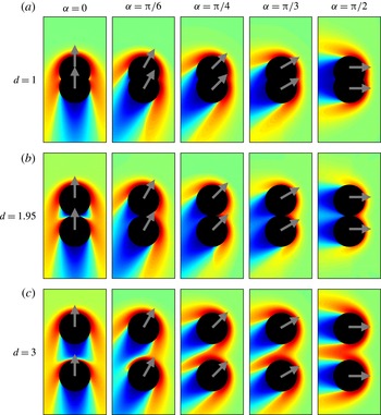
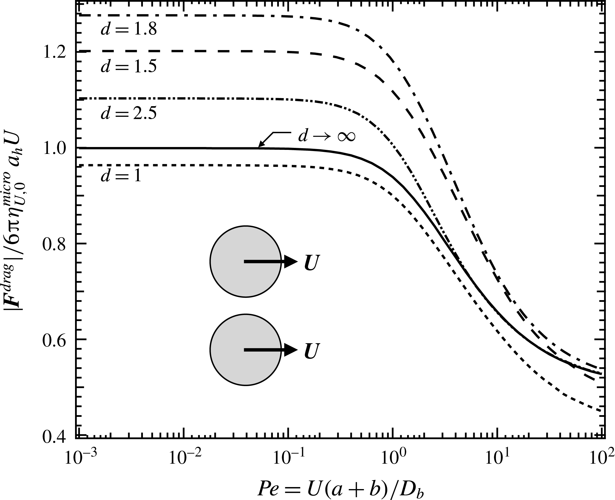
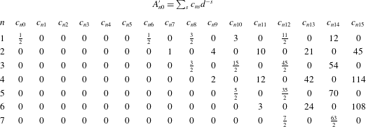
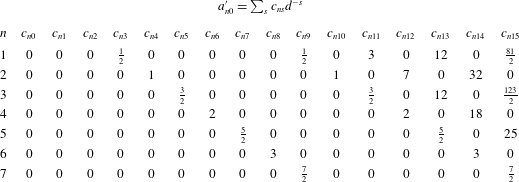
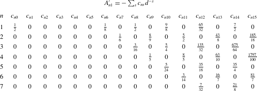
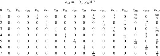
1 Introduction
The study of flow and mechanical instabilities in the sedimentation of particles through pure and complex fluids is a problem of broad scientific and technological interest. Such instabilities are diverse in their form and origin, including processes such as the gravitational collapse of colloidal gels (Poon et al. Reference Poon, Starrs, Meeker, Moussaïd, Evans, Pusey and Robins1999; Starrs et al. Reference Starrs, Poon, Hibberd and Robins2002; Padmanabhan & Zia Reference Padmanabhan and Zia2017) and vortex formation in Newtonian solvents (Tee et al. Reference Tee, Mucha, Cipelletti, Manley, Brenner, Segre and Weitz2002; Bergougnoux et al. Reference Bergougnoux, Ghicini, Guazzelli and Hinch2003). Of particular industrial interest are instabilities that arise during the sedimentation of particles through shear-thinning fluids, which are widely utilized in processes for which particle sedimentation is undesirable. Drilling fluids are a notable example; their high viscosity during slow flow aids in keeping rock cuttings suspended for extraction, but shear thinning is desirable for reducing the energy required to remove fluid from a well (Daugan et al. Reference Daugan, Talini, Herzhaft, Peysson and Allain2004). However, these beneficial properties are mitigated by a suspension instability of sedimenting particles; initially well-dispersed suspensions later rearrange and form particle-rich columns separated by particle-poor fluid regions, leading to enhanced sedimentation (Allen & Uhlherr Reference Allen and Uhlherr1989; Bobroff & Phillips Reference Bobroff and Phillips1998; Daugan et al. Reference Daugan, Talini, Herzhaft, Peysson and Allain2004; Mora, Talini & Allain Reference Mora, Talini and Allain2005). Overall, this instability increases the sedimentation rate of the particles, hindering their removal.
It has been proposed that this ‘column instability’ in shear-thinning fluids arises from non-equilibrium attractions between sedimenting pairs (Phillips Reference Phillips2010; Vishnampet & Saintillan Reference Vishnampet and Saintillan2012), a supposition supported by experimental observations of particle-pair trajectories in non-Newtonian fluids (Riddle, Narvaez & Bird Reference Riddle, Narvaez and Bird1977; Joseph et al. Reference Joseph, Liu, Poletto and Feng1994; Gumulya et al. Reference Gumulya, Horsley, Pareek and Lichti2011a ,Reference Gumulya, Horsley, Wilson and Pareek b ). While the form of the pair attraction has been observed to vary with the non-Newtonian rheology of the suspending fluid, the initial arrangement of the falling pair relative to gravity is seen to influence the behaviour of particles sedimenting with their line of centres aligned either along or transverse to the gravitational force. In the former group, particles attract toward one another (Riddle et al. Reference Riddle, Narvaez and Bird1977; Gumulya et al. Reference Gumulya, Horsley, Wilson and Pareek2011b ). In the latter group, particles sedimenting side-by-side attract and reorient such that they fall along their line of centres if they were initially closely spaced, but separate without reorienting if initially widely spaced (Joseph et al. Reference Joseph, Liu, Poletto and Feng1994; Gumulya et al. Reference Gumulya, Horsley, Pareek and Lichti2011a ). Phenomenological explanations derived empirically from experiments attribute these behaviours to features of the non-Newtonian rheology. For example, Joseph et al. (Reference Joseph, Liu, Poletto and Feng1994) hypothesize that shear-thinning fluids permit the emergence of localized reductions in viscosity, ‘corridors’ in which a second nearby particle experiences lower resistance and thus higher velocity, leading to an effective attraction between the pair. Seemingly corroborating this idea, Gheissary & Van den Brule (Reference Gheissary and Van den Brule1996) reported that no pair attractions arise between a pair of particles sedimenting through a Boger fluid. Gumulya et al. (Reference Gumulya, Horsley, Pareek and Lichti2011a ) provide still another explanation, attributing pair attraction in shear-thinning fluids to the emergence of normal stress differences. Overall, while there has been some success in explaining these interactions from a phenomenological perspective, their ultimate origin remains unclear.
Theoretical study of the interactions between pairs of particles sedimenting through complex fluids have primarily focused on continuum constitutive models. For example, Brunn (Reference Brunn1977) and later Phillips & Talini (Reference Phillips and Talini2007) utilized the second-order fluid model to show that a pair of identical spheres will attract and reorient until they fall as a doublet with their axis parallel to gravity, in qualitative agreement with experimental results for closely spaced pairs (Joseph et al. Reference Joseph, Liu, Poletto and Feng1994; Gumulya et al. Reference Gumulya, Horsley, Pareek and Lichti2011a ). Despite this apparent success, the second-order fluid model is limited to the near-equilibrium regime by its assumption of constant viscosity. It also precludes the study of non-continuum behaviour such as depletion flocculation (Asakura & Oosawa Reference Asakura and Oosawa1954) and structure-induced stabilization (Chu, Nikolov & Wasan Reference Chu, Nikolov and Wasan1996; Xu, Nikolov & Wasan Reference Xu, Nikolov and Wasan1997), owing to its assumption that the fluid interacts with the pair as a continuum. While there have been attempts to relax the near-equilibrium restriction through the use of alternative nonlinear continuum constitutive models (Feng, Huang & Joseph Reference Feng, Huang and Joseph1996; Yu, Wachs & Peysson Reference Yu, Wachs and Peysson2006; Goyal & Derksen Reference Goyal and Derksen2012), these studies have been limited in scope, e.g. focusing on sedimentation in channels. None have interrogated the role of non-equilibrium, non-continuum interactions and corresponding phenomena.
The primary focus of this investigation is to interrogate the microstructurally mediated pair-level forces between two microscopic probe particles driven at fixed velocity through a suspension of freely draining colloids. This simple model system is inspired by the single-particle active microrheology framework, which has successfully captured a wide range of non-Newtonian flow behaviours, including shear thinning and thickening (Brady & Vicic Reference Brady and Vicic1995; Bergenholtz, Brady & Vicic Reference Bergenholtz, Brady and Vicic2002; Squires & Brady Reference Squires and Brady2005; Khair & Brady Reference Khair and Brady2006; Meyer et al. Reference Meyer, Marshall, Bush and Furst2006; Sriram, Meyer & Furst Reference Sriram, Meyer and Furst2010), normal stress differences (Brady & Vicic Reference Brady and Vicic1995; Bergenholtz et al. Reference Bergenholtz, Brady and Vicic2002; Zia & Brady Reference Zia and Brady2012; Chu & Zia Reference Chu and Zia2016) and time-dependent behaviour (Khair & Brady Reference Khair and Brady2005; Zia & Brady Reference Zia and Brady2013; Swan, Zia & Brady Reference Swan, Zia and Brady2014; Mohanty & Zia Reference Mohanty and Zia2017). These non-continuum behaviours are explained at the two-body level, where a single particle interacts with the surrounding microstructure. For weak flow, dynamics are set by a balance of interparticle and Brownian forces, and the microstructure is Boltzmann distributed. This balance is upset when a flow is imposed, giving rise to hydrodynamic drag on the particles and distortion of the microstructure from its equilibrium configuration. At the two-body level, this non-equilibrium deformation depends only on the strength of the imposed flow and of the microscopic forces acting on the particles. In this simple model, hydrodynamic interactions are neglected entirely, an idealized limit that nonetheless finds application in freely draining suspensions where particles are hydrodynamically dilute, e.g. kept far apart by repulsive forces such as electrostatic interactions.
A pair interacting with a bath is at least a three-body problem, but has been treated analytically when the surrounding body is structureless and isotropic, via equilibrium statistical mechanics. The most notable result from this approach is the depletion force modelled by Asakura & Oosawa (Reference Asakura and Oosawa1954). Closely spaced probes exclude bath particles from the space between them, and the resulting osmotic pressure gradients give rise to an attractive force between the probes. When a deterministic force stronger than thermal fluctuations acts on the probes, the intervening and surrounding microstructure is distorted by flow, resulting in qualitative and quantitative changes in the microstructurally mediated forces experienced by the probes (Dzubiella, Löwen & Likos Reference Dzubiella, Löwen and Likos2003; Carpen Reference Carpen2005; Khair & Brady Reference Khair and Brady2007; Krüger & Rauscher Reference Krüger and Rauscher2007; Zia Reference Zia2011).
Pair interactions away from equilibrium have been previously studied via Brownian dynamics simulation (Carpen Reference Carpen2005; Zia Reference Zia2011), lattice gas simulations (Mejía-Monasterio & Oshanin Reference Mejía-Monasterio and Oshanin2011) and confocal microscopy experiments (Sriram & Furst Reference Sriram and Furst2012, Reference Sriram and Furst2015). Prior theoretical interrogations of such non-equilibrium interactions have been more limited in scope. For example, Dzubiella et al. (Reference Dzubiella, Löwen and Likos2003) examined non-equilibrium depletion interactions between soft colloids moving at arbitrary orientations, but their theoretical approach relied on the dynamic superposition approximation, whereby the microstructural deformation about the two probes is obtained by simply superimposing two independent structures generated by a single driven probe. This restriction limits the framework to slowly moving, widely spaced probes, precluding the study of strong departures from equilibrium, or close initial spacings. To the extent that such models might provide a connection to the column instability in polymeric shear-thinning fluids, such a restriction is severe. To overcome these limitations, Krüger & Rauscher (Reference Krüger and Rauscher2007) employed an approach in which the disturbance field is expanded in spherical harmonics, a method that proves to be numerically intractable when probe forcing is strong or probe separation is small. An alternative approach utilized by Khair & Brady (Reference Khair and Brady2007), based on transformation of the Smoluchowski equation governing microstructural distortion into the Helmholtz equation, extended the framework to moderate forcing strength and arbitrary separation distances. While these two methods relax some of the restrictions of the dynamic superposition approximation, they are limited to probes travelling along (Khair & Brady Reference Khair and Brady2007; Krüger & Rauscher Reference Krüger and Rauscher2007) or transverse (Krüger & Rauscher Reference Krüger and Rauscher2007) to their line of centres. This precludes the study of angular variations in structure arising from altering probe orientation with respect to the flow, preventing the study of the forces that cause probes to reorient and produce unstable structures in suspensions.
We have developed a theoretical framework that overcomes these limitations, allowing solution of the Smoluchowski equation for arbitrary probe velocities, probe orientations with respect to their velocities and probe separations. In the weakly nonlinear regime, we find that structural symmetries allow relation of the forces exerted on the probes to probe velocity through a set of coupling tensors similar to those of Stokes flow. When forcing strength is increased, this symmetry is lost, and new behaviours are observed. In particular, we find that our model qualitatively predicts experimentally observed instabilities in particle trajectories: closely spaced particles sedimenting side-by-side will attract and reorient such that they fall along their line of centres, while widely separated particles fall without reorienting.
The remainder of this work is organized as follows. In § 2, the model system is presented. We derive in § 3 expressions for the force the suspension exerts on the probes, and the Smoluchowski equation governing the microstructural evolution of the bath particles. Results for the non-equilibrium microstructure and the resultant forces exerted on the probes are presented in § 4. Concluding remarks are presented in § 5.
2 Model system
We consider
 $N-2$
neutrally buoyant colloidal hard spheres of hydrodynamic radius
 $b_{h}$
suspended in a solvent of viscosity
 $\unicode[STIX]{x1D702}$
and density
 $\unicode[STIX]{x1D70C}$
, through which a pair of colloidal probes of hydrodynamic radius
 $a_{h}$
are driven at fixed velocity
 $\boldsymbol{U}$
. All bath particles are free of external forces and torques. The importance of fluid inertia relative to viscous stresses, set by the Reynolds number,
 $Re=\unicode[STIX]{x1D70C}Ua/\unicode[STIX]{x1D702}$
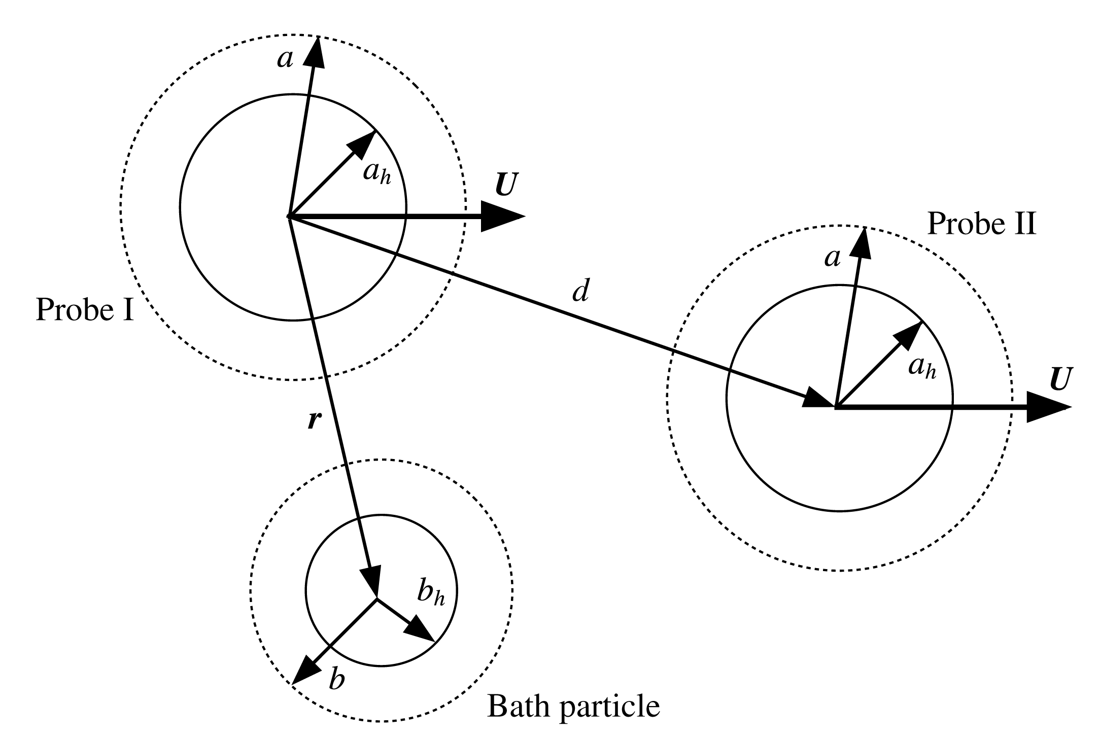
, is negligible owing to the small size of the particles. Fluid flow is thus governed by the Stokes equations, and particle motion is set by their solution and the detailed microscopic forces between the particles. This model system is illustrated in figure 1, where two probes, labelled I and II are separated by distance
 $\boldsymbol{d}$
, and interact with a bath particle at position
 $\boldsymbol{r}$
relative to probe I.
Three-body model system: two probes, I and II, interact with a bath particle.

Probe translation through the bath distorts the suspension and, simultaneously, their interactions with the deformed microstructure tend to alter probe motion. The degree to which the structure is distorted is set by the strength of the advective flow
 $U$
relative to the speed of diffusion
 $D_{b}/\ell$
that tends to restore the equilibrium microstructure, and defines a Péclet number,
 $Pe=U\ell /D_{b}$
. Here,
 $\ell$
is the characteristic length scale of distortion,
 $D_{b}=kT/6\unicode[STIX]{x03C0}\unicode[STIX]{x1D702}b_{h}$
is the diffusivity of an isolated bath particle,
 $k$
is Boltzmann’s constant and
 $T$
is the absolute temperature. Because probe velocity is prescribed to remain fixed, the encounters between probes and bath particles that would tend to change probe motion or orientation must be counteracted by the externally applied force. That is, the interplay between probe motion and the resulting changes in hydrodynamic and entropic forces exerted on the particles induces a suspension-mediated, effective force on the pair. Because the effective suspension-mediated force is set by particle interactions and the degree of microstructural distortion, its determination requires, firstly, formulation of the configuration-dependent entropic and hydrodynamic forces and, secondly, a statistical-mechanics model connecting the microstructural configuration and the average effective force. We address the configuration-dependent forces next, and the suspension-mediated forces in § 3.
2.1 Microscopic forces: interparticle repulsion and hydrodynamic interactions
The strength of hydrodynamic interactions between hard spheres can be set by tuning the range of interparticle repulsion. As repulsive interactions become long-ranged, hydrodynamic entrainment and Brownian drift weaken while flux due to hard-sphere collisions grows stronger. The excluded-annulus model (Russel Reference Russel1984) provides a convenient framework for systematically tuning the strength of hydrodynamic interactions by introducing a minimum approach distance
 $r=r_{min}$
between the probe and bath particles. This minimum approach distance is enforced by an interparticle potential
 $$\begin{eqnarray}V(r)=\left\{\begin{array}{@{}cl@{}}0, & r\geqslant r_{min},\\ \infty , & r<r_{min}.\end{array}\right.\end{eqnarray}$$
Bath-particle centres are thus excluded from a spherical volume defined by
 $r_{min}$
centred about each probe. Physically, such excluded volume interactions can arise from hard-sphere repulsion, as well as particle and solvent conditions that extend the effective size of the probe and bath particles to the thermodynamic radii
 $a$
and
 $b$
(cf. figure 1). These physical mechanisms include surface roughness, grafted polymer hairs or ionic screening layers employed to sterically stabilize a suspension, for example. The range over which the minimum approach distance
 $r_{min}=a+b$
extends beyond the hydrodynamic size dictates the strength of hydrodynamic interactions. To this end, it is convenient to define two excluded-annulus parameters
 $$\begin{eqnarray}\unicode[STIX]{x1D705}_{a}=(a-a_{h})/a_{h},\quad \unicode[STIX]{x1D705}_{b}=(b-b_{h})/b_{h},\end{eqnarray}$$
describing the strength of entrainment. When
 $\unicode[STIX]{x1D705}_{a},\unicode[STIX]{x1D705}_{b}\rightarrow 0$
, the hydrodynamic no-slip surfaces of the probes and bath particles may approach near enough to experience lubrication interactions. When
 $\unicode[STIX]{x1D705}_{a}$
,
 $\unicode[STIX]{x1D705}_{b}\sim \mathit{O}(1)$
, particles experience long-range hydrodynamic interactions. Finally, when
 $\unicode[STIX]{x1D705}_{a},\unicode[STIX]{x1D705}_{b}\rightarrow \infty$
, the no-slip surfaces always remain widely separated, and hydrodynamic entrainment is negligible. This represents an idealized limit; a finite value of
 $\unicode[STIX]{x1D705}_{a},\unicode[STIX]{x1D705}_{b}$
is required to transfer momentum between the particles via the fluid. While the freely draining approximation may seem severe, it nonetheless affords a useful approximation for behaviour of shear-thinning fluids, where, e.g. suspension viscosity changes little for
 $\unicode[STIX]{x1D705}_{a},\unicode[STIX]{x1D705}_{b}\gtrapprox 2$
(Bergenholtz et al.
Reference Bergenholtz, Brady and Vicic2002; Khair & Brady Reference Khair and Brady2006; Brady, Khair & Swaroop Reference Brady, Khair and Swaroop2006; Swaroop & Brady Reference Swaroop and Brady2007).
3 Theoretical framework
A pair of colloids immersed in a continuum solvent undergo Brownian diffusion and, in the presence of hydrodynamic interactions, also experience Brownian drift, a deterministic force that acts to drive the pair apart. Addition of particles to the system weakens both of these effects, but can introduce a new entropic force, as the many-body microscopic forces between the particles produce an effective force on the interacting pair. When these new particles are a smaller ‘depletant’ species, this deterministic force will drive the pair together. Thus, maintaining a fixed separation between a pair of colloids (either in a solvent or in a suspension) requires application of a deterministic force. The strength and direction of the required force depends on the degree to which the microstructure of the intervening medium deviates from its equilibrium configuration. This required effective force can be computed as an average over all permissible configurations of the particles; the average external force is equal in magnitude and acts opposite in direction to the suspension-mediated force exerted on the probes by the bath particles. At equilibrium, theoretical expressions for the depletion force arising in the presence of depletant particles are well known (Asakura & Oosawa Reference Asakura and Oosawa1954). The focus of the present study is to develop a theoretical model for the effective force acting on a pair of probe particles immersed in a suspension that is driven far from equilibrium by the externally driven motion of the probes, and to relate these results to the stability of the configurations of sedimenting pairs. In the present section, we develop the theoretical framework for computing this average force between a pair of colloidal probes driven at fixed velocity through a bath of colloids of arbitrary relative size. We begin with a brief review of the well-known case in which probe velocity is strictly thermal in origin and the average suspension-mediated force is given by the theory of Asakura & Oosawa (Reference Asakura and Oosawa1954). Following this, we develop the corresponding framework for arbitrary strength of external forcing relative to the Brownian force of the background particles.
3.1 Suspension-mediated force at equilibrium: depletion attractions
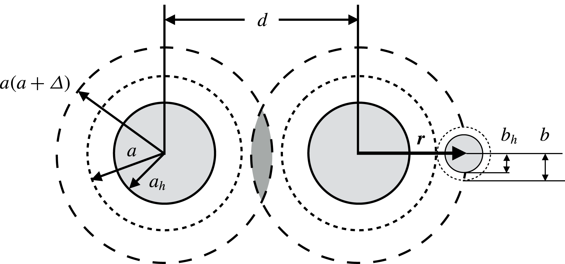
Schematic of the equilibrium depletion interaction.

We consider two microscopic probes immersed in a suspension of bath particles. At thermodynamic equilibrium, the arrangement of bath particles is given by the Boltzmann distribution
 $\unicode[STIX]{x1D70C}=n_{b}\exp (-V/kT)$
, where
 $\unicode[STIX]{x1D70C}$
is the correlation function giving the probability of finding a bath particle in a differential volume
 $\text{d}\boldsymbol{r}$
,
 $n_{b}$
is the bulk number density of the bath particles far from the probes and
 $V(\boldsymbol{r})$
is the interaction potential between a bath particle located at
 $\boldsymbol{r}$
and each probe. If the probes are widely separated, the bath-particle distribution is isotropic about each probe. However, as the probes near one another, the structure around them changes. If the probes approach closely enough, bath particles are excluded from the gap between them (cf. figure 2), reducing the configurational entropy of the suspension. To alleviate this entropic restriction, the probes move toward one another, closing the intervening gap and increasing the volume available to the bath particles. The entropic driving force that pushes the colloids together can also be viewed as an attractive force between the pair that scales with the thermal energy
 $kT$
of the bath. The depletion force, initially described by Asakura & Oosawa (Reference Asakura and Oosawa1954) for two colloids diffusing in a suspension of macromolecules of much smaller size, acting on probe I in our model system, is given by
 $$\begin{eqnarray}\frac{\boldsymbol{F}_{1}^{AO}}{n_{b}kT(a+b)^{2}}=\left\{\begin{array}{@{}ll@{}}\mathbf{0},\quad & d/2\geqslant a(1+\unicode[STIX]{x1D6E5}),\\ {\displaystyle \frac{\unicode[STIX]{x03C0}}{4}}(4-d^{2}/(a+b)^{2})\,\hat{\boldsymbol{d}},\quad & a\leqslant d/2<a(1+\unicode[STIX]{x1D6E5}),\end{array}\right.\end{eqnarray}$$
where
 $n_{b}$
is the bulk number density of the bath particles,
 $d$
is the separation between the probes,
 $\unicode[STIX]{x1D6E5}=b/a$
is the characteristic attraction length and
 $\hat{\boldsymbol{d}}$
is the unit vector pointing from probe I to the second probe. The depletion force acts with equal magnitude and opposite direction on each probe,
 $\boldsymbol{F}_{1}^{AO}=-\boldsymbol{F}_{2}^{AO}$
. When
 $d<2a(1+\unicode[STIX]{x1D6E5})$
, bath particles are excluded from the gap between the probes, and the probes attract. For
 $d>2a(1+\unicode[STIX]{x1D6E5})$
, bath particles move freely between the probes and the depletion force vanishes.
This bath particle-mediated force between the probes can also be described mechanically as a manifestation of a non-uniform osmotic pressure. The probes suffer many collisions with bath particles, giving rise to a particle osmotic pressure. When bath particles are excluded from the gap between the probes, the osmotic pressure is zero in this region, but non-zero on all other portions of their surfaces. This imbalance in osmotic pressure then drives the pair together until they reach mechanical equilibrium at contact.
More generally, any anisotropy in bath-particle configuration, such as that resulting from flow or external fields, can be expected to induce bath-particle-mediated forces on the probes, where the many-body microscopic forces that ultimately set the effective force are influenced by the imposed flow. The determination of such forces is addressed in the next section.
3.2 Suspension-mediated forces away from equilibrium: two translating probes
Here we consider the motion of a pair of probe particles driven by an external force at fixed velocity
 $\boldsymbol{U}$
through the suspension. Probe motion sets bath particles and fluid into motion, distorting the particle microstructure. In turn, the bath particles resist probe motion via hydrodynamic entertainment, interparticle potentials and Brownian forces. Each of these forces are configuration dependent and, in consequence, the forces exerted on the probes fluctuate as all permissible arrangements of the surrounding microstructure are sampled. Thus, the force required to maintain the prescribed velocity is an average over all such configurations. It is appropriate to view this average as a suspension-mediated force acting on and between the probes. In § 3.2.1 we develop expressions governing the evolving microstructure, and in § 3.2.2, we develop the theoretical framework describing the suspension-mediated force that must be counteracted to maintain fixed probe velocity.
3.2.1 Microstructural evolution
The evolution of the
 $N$
-particle probability density function
 $P_{N}(\boldsymbol{x}_{1},\boldsymbol{x}_{2},\ldots ,\boldsymbol{x}_{N},t)$
, which gives the probability of finding particle
 $i$
at position
 $\boldsymbol{x}_{i}$
, is governed by conservation of probability, the
 $N$
-body Smoluchowski equation:
 $$\begin{eqnarray}\frac{\unicode[STIX]{x2202}P_{N}}{\unicode[STIX]{x2202}t}+\mathop{\sum }_{i=1}^{N}\unicode[STIX]{x1D735}_{i}\boldsymbol{\cdot }\boldsymbol{j}_{i}=0,\end{eqnarray}$$
where
 $\boldsymbol{j}_{i}=\boldsymbol{U}_{i}P_{N}$
is the probability density flux of particle
 $i$
. In the Stokes flow regime, the velocity of particle
 $i$
is linear in the forces exerted on each particle, and arises from the external force on probe
 $j$
,
 $\boldsymbol{F}_{j}^{ext}$
, as well as Brownian and interparticle forces:
 $$\begin{eqnarray}\boldsymbol{U}_{i}=\mathop{\sum }_{j=1}^{2}\unicode[STIX]{x1D648}_{ij}\boldsymbol{\cdot }\boldsymbol{F}_{j}^{ext}-\mathop{\sum }_{j=1}^{N}\unicode[STIX]{x1D648}_{ij}\boldsymbol{\cdot }(\unicode[STIX]{x1D735}_{j}V+kT\unicode[STIX]{x1D735}_{j}\ln P_{N}),\end{eqnarray}$$
where
 $\unicode[STIX]{x1D648}_{ij}$
is the
 $N$
-body hydrodynamic mobility tensor that depends on particle positions
 $\{\boldsymbol{x}_{1},\boldsymbol{x}_{2},\ldots \boldsymbol{x}_{N}\}$
and
 $V$
is an
 $N$
-body interparticle potential. For the probes,
 $i\in [1,2]$
, and for the bath particles,
 $i\in [3,N]$
.
To study effective pair-level entropic interactions between the probes, we focus our attention on the limit
 $\unicode[STIX]{x1D705}_{a},\unicode[STIX]{x1D705}_{b}\rightarrow \infty$
, where the effects of hydrodynamic interactions can be neglected and interactions are strictly entropic in origin. In this limit, the hydrodynamic mobility tensors
 $\unicode[STIX]{x1D648}_{ij}$
are given by the isolated particle value,
 $\unicode[STIX]{x1D648}_{11}=\unicode[STIX]{x1D648}_{22}=\unicode[STIX]{x1D644}/6\unicode[STIX]{x03C0}\unicode[STIX]{x1D702}a_{h}$
for the probes and
 $\unicode[STIX]{x1D648}=\unicode[STIX]{x1D644}/6\unicode[STIX]{x03C0}\unicode[STIX]{x1D702}b_{h}$
for the bath particles, where
 $\unicode[STIX]{x1D644}$
is the identity tensor, and the particle velocity takes the form
 $$\begin{eqnarray}\boldsymbol{U}_{i}=M_{a}\boldsymbol{F}_{i}^{ext}-M_{a}\unicode[STIX]{x1D735}_{i}V-D_{a}\unicode[STIX]{x1D735}_{i}P_{N}(\boldsymbol{x}_{1},\boldsymbol{x}_{2},\ldots \boldsymbol{x}_{N}),\quad i\in [1,2]\end{eqnarray}$$
for the probes
 $$\begin{eqnarray}\boldsymbol{U}_{i}=-M_{b}\unicode[STIX]{x1D735}_{i}V-D_{b}\unicode[STIX]{x1D735}_{i}\ln P_{N}(\boldsymbol{x}_{1},\boldsymbol{x}_{2},\ldots \boldsymbol{x}_{N}),\quad i\in [3,N],\end{eqnarray}$$
where
 $D_{a}=kTM_{a}=kT/6\unicode[STIX]{x03C0}\unicode[STIX]{x1D702}b_{h}$
and
 $D_{b}=kTM_{b}=kT/6\unicode[STIX]{x03C0}\unicode[STIX]{x1D702}b_{h}$
are the Stokes–Einstein diffusivities of a probe and a bath particle, respectively. To ensure that probe velocities remain fixed at
 $\boldsymbol{U}_{1}=\boldsymbol{U}_{2}=\boldsymbol{U}$
, an external force must be applied to each probe, which is found by solving the probe velocity (3.4) for
 $\boldsymbol{F}_{i}^{ext}$
:
 $$\begin{eqnarray}\boldsymbol{F}_{i}^{ext}=6\unicode[STIX]{x03C0}\unicode[STIX]{x1D702}a_{h}\boldsymbol{U}+\unicode[STIX]{x1D735}_{i}V+kT\unicode[STIX]{x1D735}_{i}\ln P_{N}.\end{eqnarray}$$
The external force exerted on each probe drives the microstructure out of equilibrium, which is an
 $N$
-body problem, with two probes interacting with
 $N-2$
bath particles. To make analytical progress, we focus on the semi-dilute limit, where the
 $N$
-body Smoluchowski equation for
 $P_{N}$
(3.2) reduces to an effective two-body equation for the conditional pair distribution function
 $g(\boldsymbol{r}\mid \boldsymbol{d})$
(cf. appendix A):
 $$\begin{eqnarray}\boldsymbol{U}\boldsymbol{\cdot }\unicode[STIX]{x1D735}_{r}g+D_{b}\unicode[STIX]{x1D6FB}_{r}^{2}g=0,\end{eqnarray}$$
where
 $\boldsymbol{r}=\boldsymbol{x}_{3}-\boldsymbol{x}_{1}$
is the position of a bath particle relative to the first probe and
 $\boldsymbol{d}=\boldsymbol{x}_{2}-\boldsymbol{x}_{1}$
denotes probe separation. The particles are hard, and thus the interparticle potential demands no relative flux at contact:
 $$\begin{eqnarray}\boldsymbol{n}_{i}\boldsymbol{\cdot }(\unicode[STIX]{x1D735}_{r}g+\boldsymbol{U}g)=0\quad \text{on }S_{i},\end{eqnarray}$$
which naturally accounts for the non-continuum nature of colloidal dispersions by rendering the excluded volume bounded by
 $S_{i}$
inaccessible to bath particles; it is accounting for this excluded volume which gives rise to the depletion force at equilibrium. The suspension is undisturbed far from the probes:
 $$\begin{eqnarray}g\rightarrow 1\quad \text{as }r\rightarrow \infty .\end{eqnarray}$$
The governing equations and boundary conditions can be expressed in dimensionless form as
 $$\begin{eqnarray}\displaystyle \unicode[STIX]{x1D6FB}^{2}g+Pe\hat{\boldsymbol{U}}\boldsymbol{\cdot }\unicode[STIX]{x1D735}g & = & \displaystyle 0,\end{eqnarray}$$
 $$\begin{eqnarray}\displaystyle \boldsymbol{n}_{i}\boldsymbol{\cdot }(\unicode[STIX]{x1D735}g+Pe\hat{\boldsymbol{U}}g) & = & \displaystyle 0\quad \text{on }S_{i},\end{eqnarray}$$
 $$\begin{eqnarray}\displaystyle g & \rightarrow & \displaystyle 1\quad \text{as }r\rightarrow \infty ,\end{eqnarray}$$
 $$\begin{eqnarray}\boldsymbol{r}\sim a+b,\quad d\sim a+b,\quad \hat{\boldsymbol{U}}=\boldsymbol{U}/U,\end{eqnarray}$$
and a dimensionless velocity
 $Pe=U(a+b)/D_{b}$
, emerges from the scalings as the strength of advection relative to Brownian diffusion. Hereafter,
 $\boldsymbol{r}^{\ast }$
and
 $\boldsymbol{d}^{\ast }$
will be used to denote dimensional particle positions when the notation would otherwise be ambiguous. With these scalings, the excluded-volume surface
 $S_{i}$
has a dimensionless radius of unity. When
 $b/a\rightarrow 0$
, our model does not reduce to the continuum treatment of probes interacting through a structureless fluid of some effective viscosity and density; the latter can produce no relative force between spherical, same-size, equal velocity probes. This large probe, non-continuum limit is of physical interest, as it can be used to model the motion of spherical probes through polymer solutions (Krüger & Rauscher Reference Krüger and Rauscher2009). Inclusion of hydrodynamic interactions in our model could recover the continuum limit, provided the probe is smooth.
3.2.2 Non-equilibrium suspension-mediated force
In § 3.2.1, it was found that a configuration-dependent force (3.6) is needed to maintain constant probe velocity. As the probes translate, they will encounter all permissible configurations of bath particles and, on average, will experience an effective, suspension-mediated force,
 $\langle \boldsymbol{F}_{i}^{eff}\rangle$
, from interaction with the microstructure. This effective force is equal in magnitude and opposite in direction to the average of the configuration-dependent external force required to maintain probe motion:
 $$\begin{eqnarray}\langle \boldsymbol{F}_{i}^{eff}\rangle =-\langle \boldsymbol{F}_{i}^{ext}\rangle =-\int \boldsymbol{F}_{i}^{ext}P_{N}(\boldsymbol{x}_{1},\boldsymbol{x}_{2},\ldots ,\boldsymbol{x}_{N})\,\text{d}\boldsymbol{x}_{1}\,\text{d}\boldsymbol{x}_{2}\ldots \,\text{d}\boldsymbol{x}_{N}.\end{eqnarray}$$
Analysis is facilitated by adopting a coordinate system relative to probe
 $i$
, where
 $\boldsymbol{z}_{i}=\boldsymbol{x}_{i}$
is the absolute position of probe
 $i$
,
 $\boldsymbol{r}_{i}=\boldsymbol{x}_{j}-\boldsymbol{x}_{i}$
gives the position of bath particle
 $j$
relative to probe
 $i$
and
 $\boldsymbol{d}_{i}=\boldsymbol{x}_{3-i}-\boldsymbol{x}_{i}$
gives the probe separation. Substitution of (3.6) into (3.12) then gives
 $$\begin{eqnarray}\langle \boldsymbol{F}_{i}^{eff}\rangle =-6\unicode[STIX]{x03C0}\unicode[STIX]{x1D702}a_{h}\boldsymbol{U}+n_{b}\int _{r\geqslant 0}kT\unicode[STIX]{x1D735}_{r_{i}}g(\boldsymbol{r}_{i}\mid \boldsymbol{d}_{i})\,\text{d}\boldsymbol{r}_{i}+n_{b}\int _{r\geqslant 0}g(\boldsymbol{r}_{i}\mid \boldsymbol{d}_{i})\unicode[STIX]{x1D735}_{r_{i}}V\,\text{d}\boldsymbol{r}_{i}\end{eqnarray}$$
after integration over the positions of all but one bath particle (cf. appendix B). Here,
 $g(\boldsymbol{r}_{i}\mid \boldsymbol{d}_{i})$
is the conditional pair distribution function of a bath particle interacting with two probes at fixed separation
 $\boldsymbol{d}_{i}$
, and is the
 $\boldsymbol{r}_{i}$
is the position of any of the bath particles relative to the probes. Because the bath particles are mono-disperse and interact via the same potentials, each bath particle is statistically identical, and may be interchanged with any other bath particle without loss of generality.
The first term on the right-hand side of (3.13) is the Stokes drag acting on each probe as if it were alone in the solvent. The remaining terms give the effect of the bath particles on probe behaviour. The second term is the average entropic force arising from Brownian motion that tends to make the bath-particle distribution homogeneous, and becomes a surface integral via the divergence theorem that vanishes because the far-field structure is undisturbed. The third term is the interparticle force arising from hard-sphere collisions, and is set by thermal forces that separate a contacting pair, acts outwards along the line of centres of a pair, and is infinitely strong at contact owing to entropic exclusion:
 $$\begin{eqnarray}\unicode[STIX]{x1D735}_{r_{i}}V=-\boldsymbol{n}_{i}kT\unicode[STIX]{x1D6FF}(r-(a+b)).\end{eqnarray}$$
Here,
 $\boldsymbol{n}_{i}$
is the outward-facing unit normal of the excluded volume surface
 $S_{i}$
and
 $\unicode[STIX]{x1D6FF}(x)$
is the Dirac delta function. Substituting this expression into (3.13) gives
 $$\begin{eqnarray}\langle \boldsymbol{F}_{i}^{eff}\rangle =-6\unicode[STIX]{x03C0}\unicode[STIX]{x1D702}a_{h}\boldsymbol{U}-n_{b}kT\int \boldsymbol{n}_{i}g(\boldsymbol{r}_{i}\mid \boldsymbol{d}_{i};\unicode[STIX]{x1D6FC},Pe)\,\text{d}S_{i}.\end{eqnarray}$$
This is an
 $N$
-particle force, where
 $N-2$
particles (the bath particles) are indistinguishable. In writing (3.15), we have emphasized that the force exerted on the probes depends conditionally on probe separation, and depends parametrically on probe orientation and
 $Pe$
. Here,
 $\unicode[STIX]{x1D6FC}$
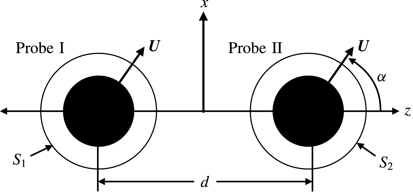
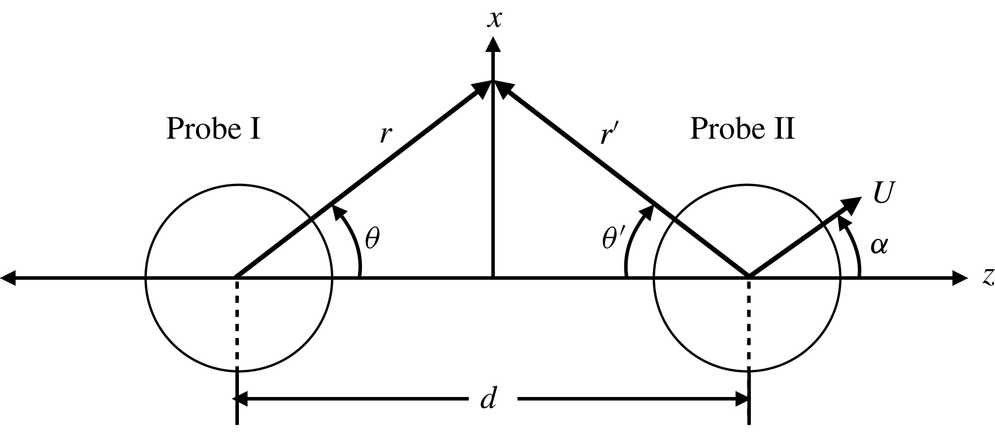
is the orientation angle characterizing the direction of travel of the probes (cf. figure 3). This angle falls between two values
 $\unicode[STIX]{x1D6FC}\in [0,\unicode[STIX]{x03C0}/2]$
. When
 $\unicode[STIX]{x1D6FC}=0$
, the probes travel along their line of centres, the ‘tandem’ orientation, while for
 $\unicode[STIX]{x1D6FC}=\unicode[STIX]{x03C0}/2$
the probes travel perpendicular to their line of centres, the ‘side-by-side’ orientation.
Coordinate system, with
 $y$
pointing out of the page. Black circles indicate probes of radius
 $a$
, solid black line indicates excluded-volume surface of radius
 $a+b$
. Probe I is located at
 $(0,0,-d/2)$
, probe II is located at
 $(0,0,d/2)$
and their excluded volume surfaces are labelled by
 $S_{\text{I}}$
and
 $S_{\text{II}}$
, respectively. Probe velocity is expressed in terms of the unit vectors
 $\boldsymbol{e}_{x}$
and
 $\boldsymbol{e}_{z}$
as
 $\boldsymbol{U}=U\sin \unicode[STIX]{x1D6FC}\boldsymbol{e}_{x}+U\cos \unicode[STIX]{x1D6FC}\boldsymbol{e}_{z}$
.

The integral term in (3.15) is the configurational average of the interparticle force. At equilibrium, this force is simply the depletion force. To examine the non-equilibrium entropic force exerted on each of the two probes by the bath particles, it is convenient to write the microstructure as a sum of its equilibrium value plus a flow-induced perturbation:
 $$\begin{eqnarray}g(\boldsymbol{r}\mid \boldsymbol{d};\unicode[STIX]{x1D6FC},Pe)=g^{eq}(\boldsymbol{r}\mid \boldsymbol{d})(1+Pe\,f(\boldsymbol{r}_{i}\mid \boldsymbol{d}_{i};\unicode[STIX]{x1D6FC},Pe)).\end{eqnarray}$$
The equilibrium microstructure
 $g^{eq}=\exp (-V/kT)$
is unity everywhere except in the excluded-volume region, where it is identically zero, and
 $f(\boldsymbol{r}_{i}\mid \boldsymbol{d}_{i};\unicode[STIX]{x1D6FC},Pe)$
represents the distortion of the equilibrium microstructure. The suspension-mediated, entropic force then becomes
 $$\begin{eqnarray}\langle \boldsymbol{F}_{i}^{eff}\rangle =-6\unicode[STIX]{x03C0}\unicode[STIX]{x1D702}a_{h}\boldsymbol{U}-n_{b}kT\int \boldsymbol{n}_{i}\,\text{d}S_{i}-Pe\,n_{b}kT\int \boldsymbol{n}_{i}f(\boldsymbol{r}_{i}\mid \boldsymbol{d}_{i};\unicode[STIX]{x1D6FC},Pe)\,\text{d}S_{i}.\end{eqnarray}$$
The first integral gives the equilibrium depletion force (3.1) exactly. The second integral gives the non-equilibrium contribution to the osmotic force,
 $$\begin{eqnarray}\langle \boldsymbol{F}_{i}^{eff,neq}\rangle \equiv -Pe\,n_{b}kT\int \boldsymbol{n}_{i}f(\boldsymbol{r}_{i}\mid \boldsymbol{d}_{i};\unicode[STIX]{x1D6FC},Pe)\,\text{d}S_{i}.\end{eqnarray}$$
In the limit of widely separated probes
 $(d=|\boldsymbol{d}_{i}|\rightarrow \infty )$
, this expression recovers the particle drag on a sphere in single-probe active microrheology in the dilute limit (Squires & Brady Reference Squires and Brady2005). In this limit, the osmotic force is directed solely along the line of forcing, and may be used to define a microviscosity via Stokes drag law (Squires & Brady Reference Squires and Brady2005)
 $$\begin{eqnarray}\unicode[STIX]{x1D702}_{U}^{micro}=-\frac{\boldsymbol{F}_{0}^{drag}\boldsymbol{\cdot }\hat{\boldsymbol{U}}}{6\unicode[STIX]{x03C0}a_{h}U},\end{eqnarray}$$
where
 $\hat{\boldsymbol{U}}=\boldsymbol{U}/|\boldsymbol{U}|$
and
 $$\begin{eqnarray}\boldsymbol{F}_{0}^{drag}=\lim _{d\rightarrow \infty }\langle \boldsymbol{F}_{i}^{eff,neq}\rangle\end{eqnarray}$$
is the particle drag force acting on a single probe. For widely separated probes, the average osmotic force is completely described by a single scalar quantity,
 $\unicode[STIX]{x1D702}_{U}^{micro}$
, depending only on the value of
 $Pe$
, and is independent of probe separation and direction of travel. It acts solely to reduce the mean speed of the probes. However, when the probes are near one another, microstructural distortions caused by one probe may influence the bath-particle distribution about the second probe. The non-equilibrium forces thus depend on probe separation
 $d$
and the strength of forcing
 $Pe$
, as well as their direction of travel with respect to their line of centres, which is characterized by an orientation angle
 $\unicode[STIX]{x1D6FC}$
.
In contrast to widely separated probes, where the non-equilibrium force acts only to reduce the mean speed of the probes, the dual-probe non-equilibrium force may also include an interactive force, a non-equilibrium analogue to the Asakura & Oosawa (Reference Asakura and Oosawa1954) depletion attraction, that may act to change the separation (or orientation) of the probes, as well as the drag force:
 $$\begin{eqnarray}\langle \boldsymbol{F}_{1}^{eff,neq}\rangle =\boldsymbol{F}^{int}+\boldsymbol{F}^{drag},\quad \langle \boldsymbol{F}_{2}^{eff,neq}\rangle =-\boldsymbol{F}^{int}+\boldsymbol{F}^{drag}.\end{eqnarray}$$
The first component, the interactive force, is defined as the force that acts to change the relative velocity between the probes:
 $$\begin{eqnarray}\boldsymbol{F}^{int}=\frac{\langle \boldsymbol{F}_{1}^{eff,neq}\rangle -\langle \boldsymbol{F}_{2}^{eff,neq}\rangle }{2}.\end{eqnarray}$$
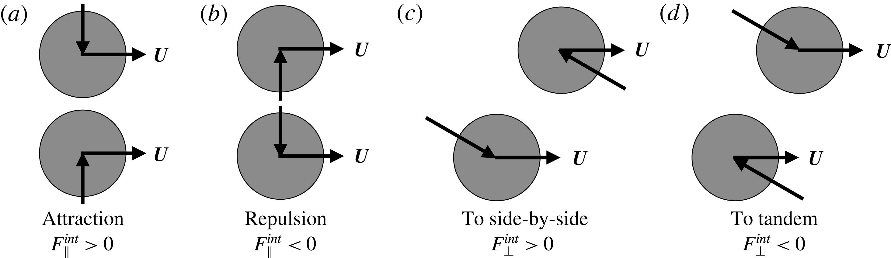
The interactive force acts with equal magnitude but opposite direction on each probe, and must be counteracted by an externally applied force to maintain the imposed probe separation and orientation. That is, it acts to change the relative velocity of the probes without influencing their average (centre-of-mass) velocity. Projection along and perpendicular to the line of centres between the probes gives
 $$\begin{eqnarray}\boldsymbol{F}^{int}=F_{\Vert }^{int}\boldsymbol{e}_{z}+F_{\bot }^{int}\boldsymbol{e}_{x},\end{eqnarray}$$
where
 $F_{\Vert }^{int}$
is the magnitude of the component of the interactive force directed along the probes’ line of centres, and
 $F_{\bot }^{int}$
is the magnitude of the force directed perpendicular to the probes’ line of centres. The physical interpretations of these components are illustrated in figure 4. The parallel component,
 $F_{\Vert }^{int}$
, tends to drive the probes together or apart. When it is positive (negative), the probes attract (repel) one another. The perpendicular force
 $F_{\bot }^{int}$
tends to reorient the probes relative to the imposed motion: either towards the tandem orientation, where the probes travel along their line of centres
 $(\unicode[STIX]{x1D6FC}=0)$
, or the side-by-side orientation
 $(\unicode[STIX]{x1D6FC}=\unicode[STIX]{x03C0}/2)$
, where motion is transverse to their line of centres. When
 $F_{\bot }^{int}>0$
, the probes seek the side-by-side orientation; when
 $F_{\bot }^{int}<0$
, the interactive force tends to realign the probes toward the tandem orientation. Whether the initial probe configuration
 $(\unicode[STIX]{x1D6FC},d)$
is stable depends on the response of
 $F_{\Vert }^{int}$
and
 $F_{\bot }^{int}$
to small perturbations in
 $\unicode[STIX]{x1D6FC}$
or
 $d$
, which will be examined in § 4.
Schematic of the interactive force,
 $\boldsymbol{F}^{int}=F_{\Vert }^{int}\boldsymbol{e}_{z}+F_{\bot }^{int}\boldsymbol{e}_{x}$
. The attractive/repulsive parallel interactive force
 $F_{\Vert }^{int}$
is shown in (a,b), and the reorientation force, the perpendicular interactive force
 $F_{\bot }^{int}$
is shown in (c,d).

The second component, the drag force, is the average of the centre-of-mass drag on each probe:
 $$\begin{eqnarray}\boldsymbol{F}^{drag}=\frac{\langle \boldsymbol{F}_{1}^{eff,neq}\rangle +\langle \boldsymbol{F}_{2}^{eff,neq}\rangle }{2}.\end{eqnarray}$$
The drag force is the same on both probes,
 $\boldsymbol{F}_{1}^{drag}=\boldsymbol{F}_{2}^{drag}=\boldsymbol{F}^{drag}$
, and must be counteracted by an externally applied force to maintain a constant centre-of-mass velocity. The magnitude of the drag force can be compared to the microstructural drag on a single probe travelling at fixed velocity through a suspension (Squires & Brady Reference Squires and Brady2005; Swan & Zia Reference Swan and Zia2013), given in (3.19) as
 $6\unicode[STIX]{x03C0}\unicode[STIX]{x1D702}_{U}^{micro}a_{h}U$
. If
 $|\boldsymbol{F}^{drag}|>6\unicode[STIX]{x03C0}\unicode[STIX]{x1D702}_{U}^{micro}a_{h}U$
, each probe encounters greater drag than were it travelling alone through the suspension. Conversely, if
 $|\boldsymbol{F}^{drag}|<6\unicode[STIX]{x03C0}\unicode[STIX]{x1D702}_{U}^{micro}a_{h}U$
, bath-mediated interaction can actually reduce the drag on each probe below the single-probe drag.
4 Results
Here we present results for the drag and interactive forces and the underlying microstructural evolution. We begin with the linear-response regime for weak probe motion in § 4.1, followed by strong external forcing in § 4.2. In each section, the governing equations for the microstructure are solved first and then are utilized to compute the effective force.
4.1 Asymptotically weak forcing
When Brownian motion is strong relative to advection, the microstructure is only weakly perturbed by probe motion, making it is natural to expand the microstructure in small
 $Pe$
:
 $$\begin{eqnarray}g(\boldsymbol{r}\mid \boldsymbol{d};\unicode[STIX]{x1D6FC},Pe)=1+Pe\,f_{1}(\boldsymbol{r}\mid \boldsymbol{d};\unicode[STIX]{x1D6FC})+Pe^{2}\,f_{2}(\boldsymbol{r}\mid \boldsymbol{d};\unicode[STIX]{x1D6FC})+\mathit{O}(Pe^{3}),\end{eqnarray}$$
where each correction
 $f_{1},f_{2},\ldots$
to the equilibrium microstructure depends conditionally on probe separation
 $\boldsymbol{d}$
with orientation
 $\unicode[STIX]{x1D6FC}$
as a parameter. The
 $\mathit{O}(Pe)$
microstructural distortion function
 $f_{1}$
satisfies Laplace’s equation:
 $$\begin{eqnarray}\displaystyle \unicode[STIX]{x1D6FB}^{2}f_{1} & = & \displaystyle 0,\end{eqnarray}$$
 $$\begin{eqnarray}\displaystyle \boldsymbol{n}_{i}\boldsymbol{\cdot }(\unicode[STIX]{x1D735}f_{1}+\hat{\boldsymbol{U}}) & = & \displaystyle 0\quad \text{on }S_{i},\end{eqnarray}$$
 $$\begin{eqnarray}\displaystyle f_{1} & \rightarrow & \displaystyle 0\quad \text{as }r\rightarrow \infty .\end{eqnarray}$$
 $f_{1}\sim \hat{\boldsymbol{U}}$
. The weakly nonlinear correction,
 $f_{2}$
, is governed by Poisson’s equation:
 $$\begin{eqnarray}\displaystyle \unicode[STIX]{x1D6FB}^{2}f_{2}+\hat{\boldsymbol{U}}\boldsymbol{\cdot }\unicode[STIX]{x1D735}f_{1} & = & \displaystyle 0,\end{eqnarray}$$
 $$\begin{eqnarray}\displaystyle \boldsymbol{n}_{i}\boldsymbol{\cdot }(\unicode[STIX]{x1D735}f_{2}+\hat{\boldsymbol{U}}f_{1}) & = & \displaystyle 0\quad \text{on }S_{i},\end{eqnarray}$$
 $$\begin{eqnarray}\displaystyle f_{2} & \rightarrow & \displaystyle 0\quad \text{as }r\rightarrow \infty .\end{eqnarray}$$
 $f_{1}$
is linear in probe velocity, both the non-homogeneous term in (4.3a
) and the no-flux boundary condition (4.3b
) are quadratic in
 $\boldsymbol{U}$
and, in consequence,
 $f_{2}\sim \hat{\boldsymbol{U}}\hat{\boldsymbol{U}}$
. Recalling from (3.17) that the scaling of the effective force is set by the non-equilibrium microstructure, the linear and weakly nonlinear contributions to the forces on each probe,
 $\langle \boldsymbol{F}_{1}^{eff}\rangle$
and
 $\langle \boldsymbol{F}_{2}^{eff}\rangle$
, scale as
 $\boldsymbol{U}$
and
 $\boldsymbol{U}\boldsymbol{U}$
.
The microstructural deformation
 $f$
can be inserted into (3.18) via (4.1) to obtain the effective force, where the linear and quadratic scalings of the structural deformation in velocity lead to a compact and revealing form:
 $$\begin{eqnarray}\frac{\langle \boldsymbol{F}_{1}^{eff,neq}\rangle }{2\unicode[STIX]{x03C0}n_{b}kT(a+b)^{2}/3}=-Pe(\hat{\unicode[STIX]{x1D64D}}_{11}+\hat{\unicode[STIX]{x1D64D}}_{12})\boldsymbol{\cdot }\hat{\boldsymbol{U}}+Pe^{2}\hat{\unicode[STIX]{x1D64F}}_{1}\boldsymbol{ : }\hat{\boldsymbol{U}}\hat{\boldsymbol{U}},\end{eqnarray}$$
for the force exerted on probe I and
 $$\begin{eqnarray}\frac{\langle \boldsymbol{F}_{2}^{eff,neq}\rangle }{2\unicode[STIX]{x03C0}n_{b}kT(a+b)^{2}/3}=-Pe(\hat{\unicode[STIX]{x1D64D}}_{22}+\hat{\unicode[STIX]{x1D64D}}_{21})\boldsymbol{\cdot }\hat{\boldsymbol{U}}+Pe^{2}\hat{\unicode[STIX]{x1D64F}}_{2}\boldsymbol{ : }\hat{\boldsymbol{U}}\hat{\boldsymbol{U}}\end{eqnarray}$$
for probe II, where the effective force is made dimensionless on the ideal osmotic force,
 $2\unicode[STIX]{x03C0}n_{b}kT(a+b)^{2}/3$
. We have defined the resistance tensors
 $\hat{\unicode[STIX]{x1D64D}}_{ij}$
, which couple the drag force exerted on probe
 $i$
to the motion of probe
 $j$
, and
 $\hat{\unicode[STIX]{x1D64F}}_{i}$
, which couple the interactive force exerted on probe
 $i$
to weakly nonlinear motion. (In general, the weakly nonlinear force on probe
 $i$
would be coupled to the three velocity dyadics of the form
 $\boldsymbol{U}_{j}\boldsymbol{U}_{k}$
through the third-rank tensors
 $\unicode[STIX]{x1D64F}_{ijk}$
, where
 $(j,k)=[(1,1),(1,2),(2,2)]$
. Here,
 $\boldsymbol{U}_{1}=\boldsymbol{U}_{2}=\boldsymbol{U}$
, meaning the force may be described by a single resistance tensor.) The subscript
 $i,j=1$
denotes probe I, and the subscript
 $i,j=2$
denotes probe II. The resistance tensors
 $\hat{\unicode[STIX]{x1D64D}}_{ij}$
are not hydrodynamic resistance tensors; rather, they are strictly entropic in origin. The symbol
 $\hat{\unicode[STIX]{x1D64D}}_{ij}$
was chosen because these tensors give the configuration-dependent resistance to probe motion arising from the distorted microstructure. For same-sized probes, the force exerted on a probe must be invariant under exchange of particle positions and labels, i.e.
 $\langle \boldsymbol{F}_{1}^{eff,neq}\rangle (\boldsymbol{d})=\langle \boldsymbol{F}_{2}^{eff,neq}\rangle (-\boldsymbol{d})$
, giving the symmetry relations
 $\hat{\unicode[STIX]{x1D64D}}_{11}=\hat{\unicode[STIX]{x1D64D}}_{22}$
,
 $\hat{\unicode[STIX]{x1D64D}}_{12}=\hat{\unicode[STIX]{x1D64D}}_{21}$
, and
 $\hat{\unicode[STIX]{x1D64F}}_{1}=-\hat{\unicode[STIX]{x1D64F}}_{2}$
. Thus, we will focus the remaining analysis on the force exerted on probe I.
The osmotic scaling of (4.4) emphasizes the physical origin of the resistance tensor, a flow-induced gradient in the osmotic pressure, and can be related to a viscous scaling set by the drag force of the bath particles in the infinite separation limit,
 $d\rightarrow \infty$
:
 $$\begin{eqnarray}\langle \boldsymbol{F}_{i}^{eff,neq}\rangle =-\frac{2\unicode[STIX]{x03C0}}{3}n_{b}kT(a+b)^{2}Pe\,\hat{\boldsymbol{U}}=-6\unicode[STIX]{x03C0}\unicode[STIX]{x1D702}_{U,0}^{micro}a_{h}\boldsymbol{U},\quad d\rightarrow \infty ,\end{eqnarray}$$
where
 $$\begin{eqnarray}\unicode[STIX]{x1D702}_{U,0}^{micro}=\unicode[STIX]{x1D702}\unicode[STIX]{x1D719}_{b}\frac{(1+\unicode[STIX]{x1D706})^{3}}{2\unicode[STIX]{x1D706}^{2}}\frac{\unicode[STIX]{x1D705}_{a}+1}{\unicode[STIX]{x1D705}_{b}+1}\end{eqnarray}$$
is the linear-response, constant-velocity microviscosity, recovering the results of Squires & Brady (Reference Squires and Brady2005), Hoh (Reference Hoh2013) and Swan & Zia (Reference Swan and Zia2013) in the infinite separation limit. Here,
 $\unicode[STIX]{x1D706}=b/a$
is the bath particle-to-probe size ratio. (For small bath particles,
 $\unicode[STIX]{x1D702}_{U,0}^{micro}\sim \mathit{O}(\unicode[STIX]{x1D719}_{b}/\unicode[STIX]{x1D706}^{2})$
, which diverges as
 $\unicode[STIX]{x1D706}\rightarrow 0$
, but this is easily resolved by noting that the condition of diluteness requires that the probes interact with only a single bath particle at a time, which requires
 $\unicode[STIX]{x1D719}_{b}/\unicode[STIX]{x1D706}^{2}\ll 1$
(Zia & Brady Reference Zia and Brady2010).) Comparison of (4.4) and (4.6) gives
 $\hat{\unicode[STIX]{x1D64D}}_{11}=\unicode[STIX]{x1D644}$
as
 $d\rightarrow \infty$
, and gives the total force exerted on probe I, scaled on Stokes drag,
 $6\unicode[STIX]{x03C0}\unicode[STIX]{x1D702}a_{h}U$
, as:
 $$\begin{eqnarray}\frac{\langle \boldsymbol{F}_{1}^{eff}\rangle }{6\unicode[STIX]{x03C0}\unicode[STIX]{x1D702}a_{h}U}=\frac{\boldsymbol{F}_{1}^{AO}}{6\unicode[STIX]{x03C0}\unicode[STIX]{x1D702}a_{h}U}-\hat{\boldsymbol{U}}-\frac{\unicode[STIX]{x1D702}_{U,0}^{micro}}{\unicode[STIX]{x1D702}}(\hat{\unicode[STIX]{x1D64D}}_{11}+\hat{\unicode[STIX]{x1D64D}}_{12})\boldsymbol{\cdot }\hat{\boldsymbol{U}}+Pe\frac{\unicode[STIX]{x1D702}_{U,0}^{micro}}{\unicode[STIX]{x1D702}}\hat{\unicode[STIX]{x1D64F}}_{1}\boldsymbol{ : }\hat{\boldsymbol{U}}\hat{\boldsymbol{U}},\end{eqnarray}$$
after insertion of (4.4) into (3.17).
Near to equilibrium, the structure of a dilute dispersion is isotropic and its rheology Newtonian. It is as though the probes move through an isotropic continuum, inspiring us to seek forms of
 $\hat{\unicode[STIX]{x1D64D}}_{11}$
and
 $\hat{\unicode[STIX]{x1D64D}}_{12}$
analogous the resistance tensors of low-
 $Re$
hydrodynamics (Brenner Reference Brenner1964). In an isotropic Newtonian fluid, the hydrodynamic resistance tensors coupling the motion a pair of spheres can be constructed from the unit vector
 $\hat{\boldsymbol{d}}$
and the isotropic unit tensor
 $\unicode[STIX]{x1D644}$
. Motion of either particle along or transverse to their line of centres can be obtained by projecting
 $\hat{\unicode[STIX]{x1D64D}}_{11}$
and
 $\hat{\unicode[STIX]{x1D64D}}_{12}$
through the orthogonal bases formed from
 $\hat{\boldsymbol{d}}\hat{\boldsymbol{d}}$
and
 $\unicode[STIX]{x1D644}$
:
 $$\begin{eqnarray}\hat{\unicode[STIX]{x1D64D}}_{ij}=R_{ij}^{\Vert }(d)\,\hat{\boldsymbol{d}}\hat{\boldsymbol{d}}+R_{ij}^{\bot }(d)(\unicode[STIX]{x1D644}-\hat{\boldsymbol{d}}\hat{\boldsymbol{d}}).\end{eqnarray}$$
Here,
 $\hat{\boldsymbol{d}}\hat{\boldsymbol{d}}$
propagates the longitudinal component of probe velocity to the force, and
 $\unicode[STIX]{x1D644}-\hat{\boldsymbol{d}}\hat{\boldsymbol{d}}$
propagates the transverse component. The probes are coupled entropically, where the motion of one distorts the suspension, producing a disturbance flux of bath particles that affects the motion of the second probe. The ‘self’ couplings
 $R_{11}^{\Vert }$
and
 $R_{11}^{\bot }$
give the force required to maintain the velocity
 $\boldsymbol{U}_{1}$
of probe I in the presence of probe II, where the fixed velocity of probe II resists the deformation of the bath needed for probe I to move. The ‘pair’ couplings
 $R_{12}^{\Vert }$
and
 $R_{12}^{\bot }$
give the force required to keep the velocity
 $\boldsymbol{U}_{1}$
from being changed by disturbance flux of bath particles created by the fixed motion of probe II. The collective resistance components
 $R^{\Vert }=R_{11}^{\Vert }+R_{12}^{\Vert }$
and
 $R^{\bot }=R_{11}^{\bot }+R_{12}^{\bot }$
give the force required to keep both probes moving through the bath in the presence of one another, i.e. the total translational drag. When the collective resistance is greater than unity, each probe experiences an increase in drag relative to that exerted by the suspension on a single probe, while values smaller than unity correspond to decreased resistance. The symmetry of the linear resistance tensors permits no relative force between two equal-velocity probes, in a manner analogous to the reversible interactions of Stokes flow.
In contrast, we find that forces that tend to produce relative motion between the probes do emerge from the weakly nonlinear coupling
 $\hat{\unicode[STIX]{x1D64F}}_{1}$
. Projection of
 $\hat{\unicode[STIX]{x1D64F}}_{1}$
through the orthogonal bases formed by
 $\hat{\boldsymbol{d}}\hat{\boldsymbol{d}}\hat{\boldsymbol{d}}$
,
 $\hat{\boldsymbol{d}}\unicode[STIX]{x1D644}$
, and
 $\unicode[STIX]{x1D644}\hat{\boldsymbol{d}}$
gives
 $$\begin{eqnarray}\hat{\unicode[STIX]{x1D64F}}_{1}=T^{\Vert }(d)\,\hat{\boldsymbol{d}}\hat{\boldsymbol{d}}\hat{\boldsymbol{d}}+T^{\bot }(d)\,\hat{\boldsymbol{d}}(\unicode[STIX]{x1D644}-\hat{\boldsymbol{d}}\hat{\boldsymbol{d}})+T^{\times }(d)2(\unicode[STIX]{x1D644}-\hat{\boldsymbol{d}}\hat{\boldsymbol{d}})\,\hat{\boldsymbol{d}}.\end{eqnarray}$$
Because
 $\hat{\unicode[STIX]{x1D64F}}_{1}=-\hat{\unicode[STIX]{x1D64F}}_{2}$
, this coupling gives rise to a force that acts equal in magnitude and opposite in direction on each probe, the interactive force (cf. (3.22), § 3.2.2). The orthogonal projections in (4.10) propagate probe motion to components of the interactive force; the scalar functions
 $T^{\Vert }$
and
 $T^{\bot }$
transform probe motion in any direction into attractive or repulsive forces that tend to drive the probes together or apart. When these couplings are both positive, the probes attract one another, but repel each other when
 $T^{\Vert },T^{\bot }<0$
. If the two have opposite signs, probe orientation
 $\unicode[STIX]{x1D6FC}$
determines whether the probes will attract or repel:
 $$\begin{eqnarray}\frac{F_{\Vert }^{int}/Pe^{2}}{n_{b}kT(a+b)^{2}}=\frac{2\unicode[STIX]{x03C0}}{3}(T^{\Vert }\cos ^{2}\unicode[STIX]{x1D6FC}+T^{\bot }\sin ^{2}\unicode[STIX]{x1D6FC}).\end{eqnarray}$$
The third coupling,
 $T^{\times }$
, gives the tendency for a pair of probes to reorient in response to the flow (cf. figure 4):
 $$\begin{eqnarray}\frac{F_{\bot }^{int}/Pe^{2}}{n_{b}kT(a+b)^{2}}=\frac{2\unicode[STIX]{x03C0}}{3}T^{\times }\sin 2\unicode[STIX]{x1D6FC}.\end{eqnarray}$$
The coupling tensors
 $\hat{\unicode[STIX]{x1D64D}}_{11}$
,
 $\hat{\unicode[STIX]{x1D64D}}_{12}$
and
 $\hat{\unicode[STIX]{x1D64F}}_{1}$
are configuration dependent, and thus require determination of the microstructural disturbance functions
 $f_{1}$
and
 $f_{2}$
. The methods for obtaining the three tensors depend on probe separation; for
 $d>2$
, we obtain analytical expressions via a twin-multipole expansion of the microstructure, as presented in appendices C and D. For
 $d<2$
, overlap of the excluded-volume surfaces of the probes demands numerical solution of the equations governing the structure utilising the finite difference method presented in appendix E.
4.1.1 Microstructure: linear and weakly nonlinear response
The linear response and weakly nonlinear microstructural distortions were computed in the present study utilizing two methods: analytically via a twin-multipole expansion for probe separations
 $d>2$
, and numerically via finite difference methods for arbitrary probe separations, as shown in appendices C–E. We begin with a discussion of the analytical results for the weakly nonlinear microstructure, followed by a comparison to our numerical results.
For separations
 $d>2$
, the
 $\mathit{O}(Pe)$
microstructural disturbance
 $f_{1}$
may be written as a twin-multipole expansion (cf. appendix C), comprising of an infinite series of multipole moments centred at probe I and a second expansion centred at probe II. While the full expansion is necessary to satisfy the no-flux boundary condition on each probe, computation of the
 $\mathit{O}(Pe)$
force on probe I requires only the dipole moment
 $(n=1)$
of the multipole expansion centred at probe I. This dipole moment is identical to the dipole moment centred about probe II, and is given in vector notation for arbitrary orientation as
 $$\begin{eqnarray}f_{1,\text{I}}^{dipole}=\frac{\boldsymbol{r}}{r^{3}}\boldsymbol{\cdot }((A_{10}^{\prime }-a_{10}^{\prime })\,\hat{\boldsymbol{d}}\hat{\boldsymbol{d}}-(A_{11}^{\prime }+a_{11}^{\prime })(\unicode[STIX]{x1D644}-\hat{\boldsymbol{d}}\hat{\boldsymbol{d}}))\boldsymbol{\cdot }\hat{\boldsymbol{U}},\end{eqnarray}$$
where the subscripts
 $1,\text{I}$
correspond to the first perturbation to the structure about probe I. Expansion of the coefficients in a Taylor series about
 $d\rightarrow \infty$
then gives
 $$\begin{eqnarray}f_{1,\text{I}}^{dipole}=\frac{\boldsymbol{r}}{2r^{3}}\boldsymbol{\cdot }\left(\unicode[STIX]{x1D644}+\frac{\unicode[STIX]{x1D644}-3\hat{\boldsymbol{d}}\hat{\boldsymbol{d}}}{2d^{3}}+\frac{\unicode[STIX]{x1D644}+3\hat{\boldsymbol{d}}\hat{\boldsymbol{d}}}{4d^{6}}\right)\boldsymbol{\cdot }\hat{\boldsymbol{U}}+O\left(\frac{1}{d^{8}}\right),\end{eqnarray}$$
consistent with the
 $\mathit{O}(1/d^{3})$
results of Krüger & Rauscher (Reference Krüger and Rauscher2007). Here, we have kept the three most physically significant terms: an isotropic term, a term decaying as
 $1/d^{3}$
and a term decaying as
 $1/d^{6}$
. Further terms in the Taylor expansion, as well as higher-order (quadrupole, octupole, etc.) moments are tabulated in appendix C.
As
 $d\rightarrow \infty$
, only the isotropic term remains, recovering the
 $\mathit{O}(Pe)$
microstructure of a single probe moving through a suspension (Squires & Brady Reference Squires and Brady2005). The terms scaling as
 $1/d^{3}$
and
 $1/d^{6}$
arise from probe interactions through the medium, and vary with probe orientation as
 $\cos \unicode[STIX]{x1D6FC}=\hat{\boldsymbol{d}}\boldsymbol{\cdot }\hat{\boldsymbol{U}}$
. Physically, the motion of probe II through the suspension distorts the surrounding microstructure, giving rise to a diffusive flux of bath particles that in turn interacts with probe I by inducing bath-particle collisions on its surface. Essentially, the bath particles act as an effective medium, influencing the motion of probe I via their flux. This is analogous to hydrodynamic entrainment, where a particle sets the fluid into motion, which in turn influences the motion of a second particle. As such, we term the interactions mediated via bath-particle flux entropic entrainment. Entropic entrainment can either hinder or enhance probe motion, depending on the direction of bath-particle flux, and manifests as a
 $1/d^{3}$
disturbance to the structure about probe I (second term in (4.14)). At the same time, the motion of probe I generates the same flux, entraining probe II with a
 $1/d^{3}$
disturbance to its structural deformation. Similar in ethos to reflection of hydrodynamic interactions through pure solvent between two spheres, this disturbance flux triggers an infinitude of reflected bath-particle interactions, leading to the
 $1/d^{6}$
and higher-order terms in (4.14).
Whether the disturbances hinder or facilitate probe motion depends on the orientation of the probes. In the tandem orientation (
 $\hat{\boldsymbol{d}}\boldsymbol{\cdot }\hat{\boldsymbol{U}}=1$
), the structural distortion about each probe is reduced relative to that of a single probe, i.e. the probes shield one another from the bath particles. Physically, the lead probe generates a depleted region behind it, reducing the structural drag on the trailing probe, while at the same time the trailing probe generates a flux of bath particles toward the leading probe, reducing the drag on the leading probe by an equivalent amount. In the side-by-side orientation
 $(\hat{\boldsymbol{d}}\boldsymbol{\cdot }\hat{\boldsymbol{U}}=0)$
, each probe accumulates particles in the upstream region into which the other probe must travel, with two consequences: increased structural drag and pressure on both probes, and more pronounced downstream depletion. Overall, the probes entrain one another via the bath particles to slow each other down.
Bath-particle advection arises in the second-order correction to the microstructure: the
 $\mathit{O}(Pe^{2})$
microstructural distortion
 $f_{2}$
. While the algebraic complexity of the multipole expansion of
 $f_{2}$
necessitates numerical solution for arbitrary probe separation (cf. appendix E), we have computed the
 $\mathit{O}(Pe^{2})$
multipole expansion about each probe in the limit of large separations. To illustrate the flux/motion interplay, the multipole expansion about probe I was found here to be
 $$\begin{eqnarray}\displaystyle f_{2,\text{I}} & = & \displaystyle \frac{\hat{\boldsymbol{U}}}{4}\boldsymbol{\cdot }\left\{\left(\frac{\unicode[STIX]{x1D644}}{r}-\frac{1}{3}\left[\frac{\unicode[STIX]{x1D644}}{r^{3}}-3\frac{\boldsymbol{r}\boldsymbol{r}}{r^{5}}\right]-\frac{\boldsymbol{r}\boldsymbol{r}}{r^{3}}\right)\boldsymbol{\cdot }\left(\unicode[STIX]{x1D644}+\frac{\unicode[STIX]{x1D644}-3\hat{\boldsymbol{d}}\hat{\boldsymbol{d}}}{2d^{3}}\right)\right\}\boldsymbol{\cdot }\hat{\boldsymbol{U}}\nonumber\\ \displaystyle & & \displaystyle +\,\frac{\boldsymbol{r}}{8r^{3}}\boldsymbol{\cdot }\left(\frac{\hat{\boldsymbol{d}}\unicode[STIX]{x1D644}-3\hat{\boldsymbol{d}}\hat{\boldsymbol{d}}\hat{\boldsymbol{d}}}{d^{2}}\right)\boldsymbol{ : }\hat{\boldsymbol{U}}\hat{\boldsymbol{U}}+O\left(\frac{1}{d^{3}}\right),\end{eqnarray}$$
and about probe II to be
 $$\begin{eqnarray}\displaystyle f_{2,\text{II}} & = & \displaystyle \frac{\hat{\boldsymbol{U}}}{4}\boldsymbol{\cdot }\left\{\left(\frac{\unicode[STIX]{x1D644}}{r^{\prime }}-\frac{1}{3}\left[\frac{\unicode[STIX]{x1D644}}{{r^{\prime }}^{3}}-3\frac{\boldsymbol{r}^{\prime }\boldsymbol{r}^{\prime }}{{r^{\prime }}^{5}}\right]-\frac{\boldsymbol{r}^{\prime }\boldsymbol{r}^{\prime }}{{r^{\prime }}^{3}}\right)\boldsymbol{\cdot }\left(\unicode[STIX]{x1D644}+\frac{\unicode[STIX]{x1D644}-3\hat{\boldsymbol{d}}\hat{\boldsymbol{d}}}{2d^{3}}\right)\right\}\boldsymbol{\cdot }\hat{\boldsymbol{U}}\nonumber\\ \displaystyle & & \displaystyle -\,\frac{\boldsymbol{r}^{\prime }}{8{r^{\prime }}^{3}}\boldsymbol{\cdot }\left(\frac{\hat{\boldsymbol{d}}\unicode[STIX]{x1D644}-3\hat{\boldsymbol{d}}\hat{\boldsymbol{d}}\hat{\boldsymbol{d}}}{d^{2}}\right)\boldsymbol{ : }\hat{\boldsymbol{U}}\hat{\boldsymbol{U}}+O\left(\frac{1}{d^{3}}\right),\end{eqnarray}$$
where
 $\boldsymbol{r}^{\prime }=\boldsymbol{r}-\boldsymbol{d}$
is the position of a bath particle relative to probe II. When
 $d\rightarrow \infty$
(no probe/probe interactions), the first terms in braces in (4.15) and (4.16) recover the
 $\mathit{O}(Pe^{2})$
weakly nonlinear correction to the microstructure about a single probe (Khair & Brady Reference Khair and Brady2006; Zia & Brady Reference Zia and Brady2010).
In both (4.15) and (4.16), the first term,
 $\hat{\boldsymbol{U}}\boldsymbol{\cdot }\{\cdot \}\boldsymbol{\cdot }\hat{\boldsymbol{U}}$
, and the second term,
 $(\cdot )\boldsymbol{ : }\hat{\boldsymbol{U}}\hat{\boldsymbol{U}}$
, capture distinct physical phenomena. The former arises from the
 $\mathit{O}(1/d^{3})$
term of
 $f_{1}$
, which is identical about each probe, and thus cannot lead to net particle accumulation or depletion between the probes; depletion behind the leading probe will be balanced by accumulation in front of the trailing probe. In contrast, the latter term in each differs by a sign, indicating that accumulation (depletion) behind the leading probe arising from this term is enhanced by accumulation (depletion) in front of the trailing probe. Thus, the second term in (4.15) and (4.16) encode the strength of particle accumulation (or depletion) between the probes. Whether bath particles accumulate or are depleted depends on the probe orientation,
 $\unicode[STIX]{x1D6FC}$
. In the tandem orientation,
 $\unicode[STIX]{x1D6FC}=0$
, the leading probe shields the trailing probe, reducing the advective flux of bath particles toward the trailing probe, which in turn leads to bath-particle depletion between the probes. In the side-by-side orientation,
 $\unicode[STIX]{x1D6FC}=\unicode[STIX]{x03C0}/2$
, the diffusion of bath particles passing between the two probes is sterically hindered, giving rise to bath-particle accumulation between the probes. In general, the magnitude of accumulation (or depletion) depends on the quantity
 $$\begin{eqnarray}(\boldsymbol{I}-\hat{\boldsymbol{d}}\hat{\boldsymbol{d}})\boldsymbol{ : }\hat{\boldsymbol{U}}\hat{\boldsymbol{U}}=1-3\cos ^{2}\unicode[STIX]{x1D6FC},\end{eqnarray}$$
where positive values give rise to accumulation, and negative values to depletion. Thus, to leading order, there can be no net accumulation or depletion between the probes when
 $\unicode[STIX]{x1D6FC}=\cos ^{-1}(1/\sqrt{3})$
.
Analysis of the expressions obtained for linear and weakly nonlinear microstructural distortions leads to two key observations: microstructural distortions about two probes travelling in the tandem orientation are reduced relative to a single probe by shielding effects, while structural distortions about probes travelling in the side-by-side orientation are enhanced. For probe separation
 $d<2$
, the Smoluchowski equation must be solved numerically, as was shown in appendices C and D.
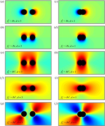
Contour plots of two probes driven weakly (
 $Pe\ll 1$
) through the suspension. Top two rows: parallel and perpendicular components of the
 $\mathit{O}(Pe)$
microstructure row separations
 $d=3$
(a,b) and
 $d=1$
(c,d). Bottom three rows: parallel, perpendicular and skew components of the
 $\mathit{O}(Pe^{2})$
microstructure for separations
 $d=3$
(e–g) and
 $d=1$
(h–j). The microstructure varies smoothly from strong depletion in blue to strong accumulation in red, with green representing the equilibrium, unperturbed structure, while the black circles represent the excluded-volume surfaces of the probes.

To obtain solutions for the perturbed microstructure for arbitrary separations
 $d$
, we note that the weakly nonlinear microstructure may be written in terms of five orientation-independent functions (cf. appendices C and D):
 $$\begin{eqnarray}\displaystyle f_{1}(\boldsymbol{r}\mid \boldsymbol{d};\unicode[STIX]{x1D6FC}) & = & \displaystyle \cos \unicode[STIX]{x1D6FC}f_{1}^{\Vert }(\boldsymbol{r}\mid \boldsymbol{d})+\sin \unicode[STIX]{x1D6FC}f_{1}^{\bot }(\boldsymbol{r}\mid \boldsymbol{d}),\end{eqnarray}$$
 $$\begin{eqnarray}\displaystyle f_{2}(\boldsymbol{r}\mid \boldsymbol{d};\unicode[STIX]{x1D6FC}) & = & \displaystyle \cos ^{2}\unicode[STIX]{x1D6FC}f_{2}^{\Vert }(\boldsymbol{r}\mid \boldsymbol{d})+\sin ^{2}\unicode[STIX]{x1D6FC}f_{2}^{\bot }(\boldsymbol{r}\mid \boldsymbol{d})+\sin 2\unicode[STIX]{x1D6FC}f_{2}^{\times }(\boldsymbol{r}\mid \boldsymbol{d}).\end{eqnarray}$$
 $d=1$
and
 $d=3$
. These two values of
 $d$
are chosen to illustrate the influence of excluded-volume interactions as probe separation is decreased from
 $d=3$
to
 $d=1$
. Contour plots in the left column correspond to
 $d=3$
; the parallel microstructural contributions
 $f_{1}^{\Vert }$
and
 $f_{2}^{\Vert }$
, shown in plots (a,e), exhibit a decrease in bath-particle density in the region between the probes, while the perpendicular components
 $f_{1}^{\bot }$
and
 $f_{2}^{\bot }$
, shown in plots (b,f), exhibit an increase, in agreement with our analytical expressions. In contrast, the microstructural distortion contour plot for
 $d=1$
(figure 5
c,d,h,i,j) differ qualitatively, because, when
 $d<2$
, the excluded-volume surfaces of the probes overlap and bath particles cannot enter the intervening gap, giving a microstructural distortion that resembles that of an isolated, non-spherical probe. This highlights the two competing mechanisms of probe interaction: for closely spaced probes, excluded-volume effects exert a much stronger influence on the microstructure, and hence the force exerted on the probes, than probe–probe interactions through the bath.
4.1.2 Drag force in the linear-response regime
For asymptotically weak forcing, the
 $\mathit{O}(Pe)$
(linear response) force exerted on each of the probes by the bath particles is linearly related to probe velocity by the resistance tensors
 $\hat{\unicode[STIX]{x1D64D}}_{11}$
and
 $\hat{\unicode[STIX]{x1D64D}}_{12}$
. These tensors exhibit the same symmetries of Stokes flow, with the important implication that the leading-order interactions can produce no relative force between two same-size, same velocity probes. That is, there is no
 $\mathit{O}(Pe)$
tendency for the probes to attract or repel one another; the linear-response force is a drag force that acts to slow centre-of-mass probe motion. Insertion of (4.4) and (4.5) into (3.24) gives the drag force in the linear-response regime in terms of these tensors as
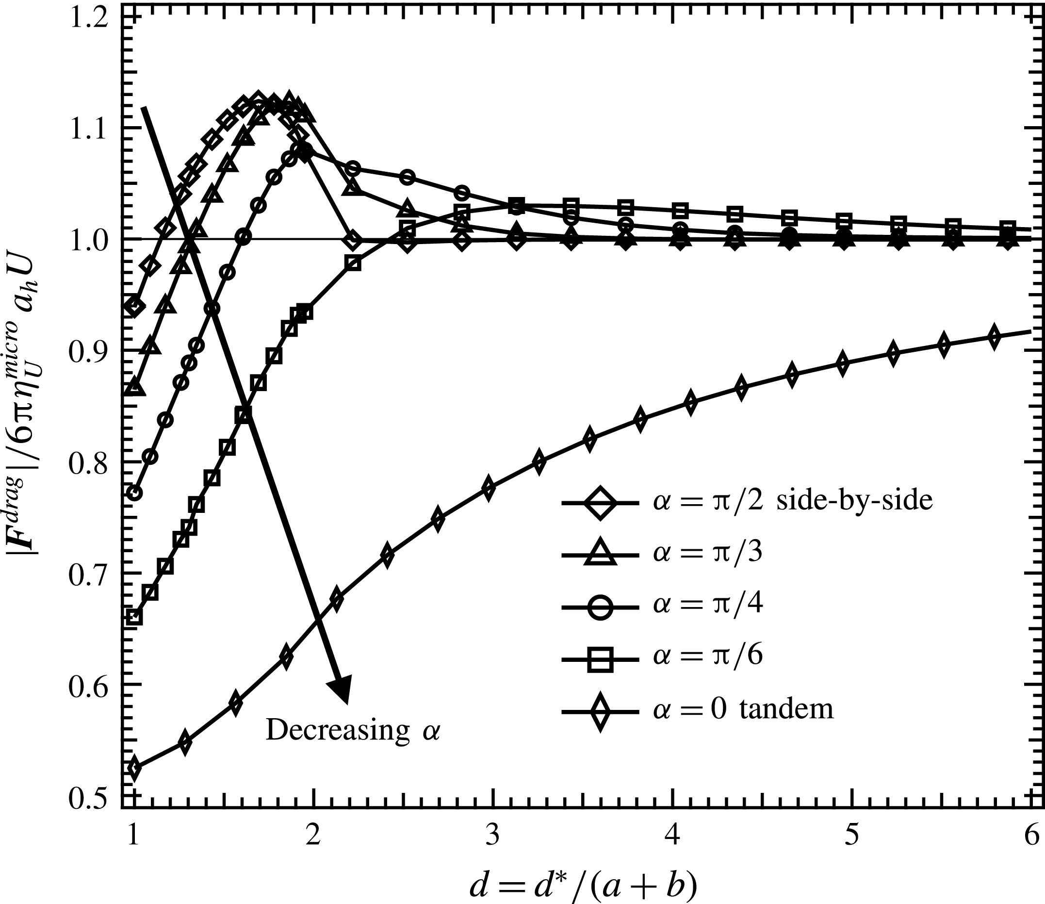
 $$\begin{eqnarray}\frac{|\boldsymbol{F}^{drag}|}{6\unicode[STIX]{x03C0}\unicode[STIX]{x1D702}_{U,0}^{micro}a_{h}U}=\sqrt{\cos ^{2}\unicode[STIX]{x1D6FC}(R_{11}^{\Vert }+R_{12}^{\Vert })^{2}+\sin ^{2}\unicode[STIX]{x1D6FC}(R_{11}^{\bot }+R_{12}^{\bot })^{2}}.\end{eqnarray}$$
We derived analytical expressions for the four resistance functions in (4.19), which can be found in appendix C. The drag force
 $|\boldsymbol{F}^{drag}|$
, normalized on the single-probe drag
 $6\unicode[STIX]{x03C0}\unicode[STIX]{x1D702}_{U,0}^{micro}U$
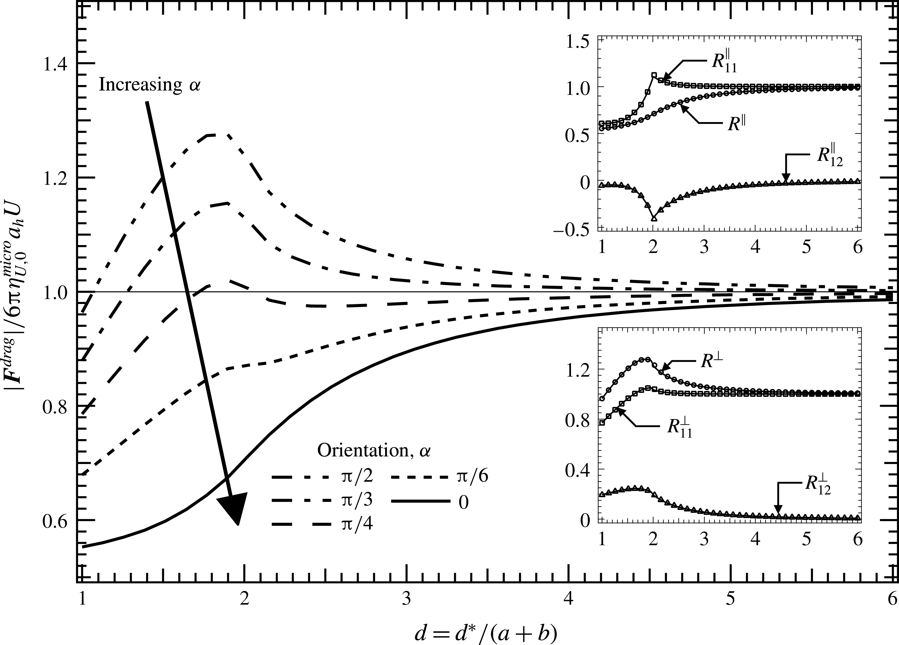
, is plotted along with the four resistance functions as a function of probe separation in figure 6 for several orientations
 $\unicode[STIX]{x1D6FC}$
.
Drag force in linear-response regime as it varies with probe separation. Main figure: force obtained from numerical solutions of (4.2) for several orientations
 $\unicode[STIX]{x1D6FC}$
. Inset: scalar resistance functions coupling drag to velocity. (Solid lines are analytical solutions; open symbols are numerical solutions.)

In the tandem orientation (
 $\unicode[STIX]{x1D6FC}=0$
, solid curve in figure 6), the drag force exerted on each of the probes by the deformed microstructure is strictly weaker than that exerted on a single probe driven through the suspension by the same external force, showing that tandem motion of two probes is easier for each than for one alone. Physically, this drag reduction arises when the trailing probe travels into the region of reduced bath-particle density following the leading probe (cf. figure 5). This shielding effect becomes more pronounced with decreased probe separation, leading to a corresponding monotonic reduction of drag with decreasing probe separation. In fact, the rate of drag reduction speeds up as the probes get closer, until
 $d=2$
, after which the reduction slows.
Side-by-side (
 $\unicode[STIX]{x1D6FC}=\unicode[STIX]{x03C0}/2$
) probe translation produces qualitatively different behaviour. When the pair are not close,
 $d>2$
, the microstructural drag on each probe is greater than that on a single probe translating under the same external force. The drag increases with decreasing separation, owing to an increase in bath-particle density about each probe, particularly in the region between them (cf. figure 5). However, this trend reverses as the probes get closer: for
 $d<2$
, the drag force decreases with decreasing probe separation, due to the exclusion of bath particles from the intervening gap between the probes (cf. figure 5); the reduction of collisions mitigates drag. Finally, for separations
 $d\lesssim 1.1$
it becomes easier for the two probes to move together than one alone. Overall, it is harder for two probes in the side-by-side orientation to move together than if they travelled alone through the suspension, except when they travel so close together that they shield one another from collisions.
Comparison of the two limits,
 $\unicode[STIX]{x1D6FC}=0$
and
 $\unicode[STIX]{x1D6FC}=\unicode[STIX]{x03C0}/2$
, reveals that it is always easier for a pair of probes to move in the tandem orientation than in the side-by-side orientation; that is, there is an energetic penalty associated with side-by-side motion as evidenced by the higher rate of effective viscous dissipation. The penalty is small for widely separated probes, and increases as the probes get closer until a maximum is reached near
 $d\simeq 1.8$
. The probes can reduce this energetic cost in one of two ways: by travelling together or apart, or by reorientation toward the tandem configuration, during which they will each experience a monotonic decrease of the drag force (cf. figure 6). As will be discussed next in § 4.1.3, both of these behaviours mitigate the energetic penalty of side-by-side translation in the weakly nonlinear-response regime.
4.1.3 Interactive force in the weakly nonlinear regime: relative motion
Relative probe motion – reorientation and attraction or repulsion – first emerges in the weakly nonlinear regime. The
 $\mathit{O}(Pe^{2})$
bath particle-mediated force is given by the third-rank weakly nonlinear resistance tensor
 $\hat{\unicode[STIX]{x1D64F}}_{1}$
which couples the interactive force to weakly nonlinear motion. We showed that, after an orthogonal decomposition,
 $\hat{\unicode[STIX]{x1D64F}}_{1}$
is described by three scalar coupling coefficients, which propagate the parallel and perpendicular interactive force as given by (4.11)–(4.12). We obtained analytical expressions for the three scalar coefficients appearing in (4.11) and (4.12), which can be found in appendix D.
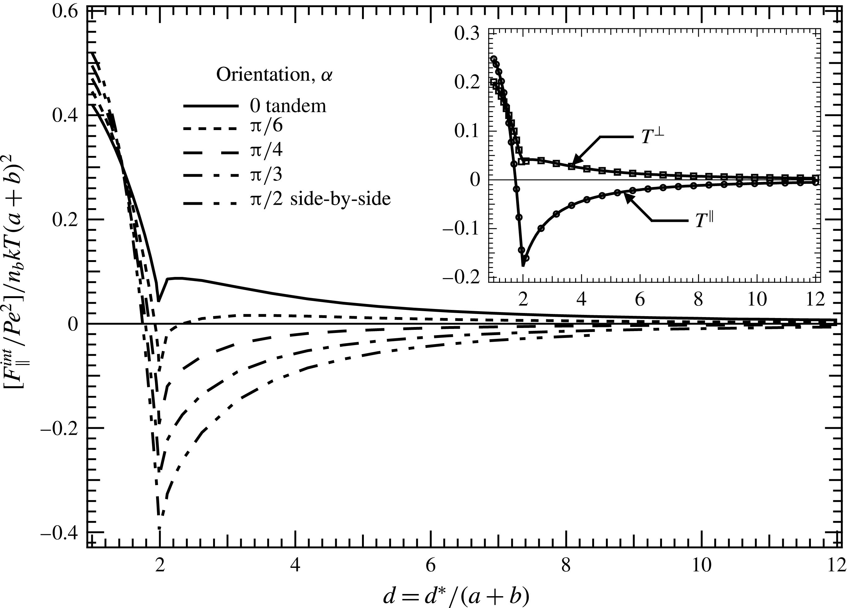
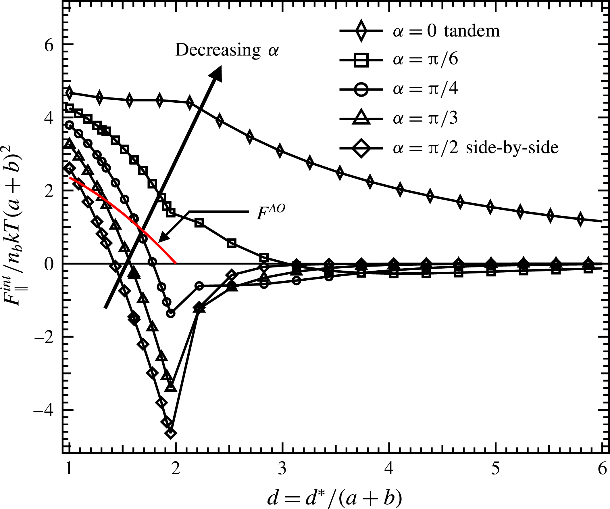
Attractive/repulsive interactive force in weakly nonlinear regime as it varies with probe separation. Main figure: force obtained from numerical solutions of (4.3) for several orientations
 $\unicode[STIX]{x1D6FC}$
. Inset: scalar resistance functions coupling interactive force to velocity. (Solid lines are analytical solutions; open symbols are numerical solutions.)

The parallel interactive force that tends to produce relative motion – attraction or repulsion – as well as the resistance coefficients
 $T^{\Vert }$
and
 $T^{\bot }$
, are plotted in figure 7, which shows that the attractive or repulsive nature of the parallel interactive force depends both on probe separation
 $d$
and orientation
 $\unicode[STIX]{x1D6FC}$
. Interactions in the tandem orientations
 $(\unicode[STIX]{x1D6FC}=0)$
are strictly attractive for all separations; physically, this arises due to collision shielding of the trailing probe by the leading probe. Because the lead probe experiences more head-on collisions with bath particles than does the trailing probe, the result is an effective non-equilibrium attraction. However, the attraction strength is non-monotonic in probe separation; it first increases with decreasing separation (moving right to left in figure 7) until a local maximum is reached at
 $d\simeq 2.4$
. At this close proximity, the space available for bath particles is severely restricted by the two nearby no-flux surfaces of the probes, and they accumulate there. For separations
 $d<2$
, bath particles are excluded entirely from the gap between the probes, and the resulting imbalance in osmotic pressure leads to a pronounced increase in attraction strength, in a manner similar to the equilibrium depletion force.
The interactive force in the side-by-side orientation
 $(\unicode[STIX]{x1D6FC}=\unicode[STIX]{x03C0}/2)$
is qualitatively different from that in the tandem orientation and also from the equilibrium depletion force, both of which are strictly attractive. In the side-by-side orientation, first the probes repel, then they attract as they approach one another. Physically, bath particles near the outboard surfaces of the probes may diffuse freely away, while particles between the probes accumulate as they struggle to migrate through the constrained gap between the probes, and the increased osmotic pressure acts to drive the probes apart. This intensifies as the gap shrinks until it becomes small enough to exclude bath particles entirely
 $(d=2)$
. Beyond this, the gap is dilute relative to the bath, reducing the repulsion strength until interactions become attractive for separations
 $d\lesssim 1.8$
. This produces a
 $Pe^{2}$
-small enhancement to or reduction of the
 $\mathit{O}(1)$
equilibrium depletion force. However, it acts over a much longer range of many particle lengths. This long-ranged repulsion, when coupled with the long-ranged attractions in the tandem orientation, may give rise to the formation of particle-rich columns or long particle chains in dense suspensions.
Between these two limits,
 $0<\unicode[STIX]{x1D6FC}<\unicode[STIX]{x03C0}/2$
, the curves show a smooth transition from pure attraction behaviour to the separation-dependent repulsive/attractive behaviour. Of note is the tendency for the most repulsive configurations to become the most attractive as
 $d\rightarrow 1$
, suggesting a tendency to reorient, discussed next.
Reorientation force in the weakly nonlinear regime, scaled on
 $\sin 2\unicode[STIX]{x1D6FC}$
, as it varies with probe separations. (Solid lines obtained from analytical solution of (4.3); open symbols are numerical solutions.)

Beyond attraction and repulsion, a tendency to reorient emerges at
 $\mathit{O}(Pe^{2})$
, and this force, (cf. (4.12)), is projected from the velocity onto the force by the scalar resistance function
 $T^{\times }$
. As such, varying
 $\unicode[STIX]{x1D6FC}$
only serves to change the magnitude of the reorientation force. The reorientation force
 $F_{\bot }^{int}$
is plotted in figure 8, scaled on
 $\sin 2\unicode[STIX]{x1D6FC}$
. The force is strictly negative for all separations. This implies that the tandem orientation is stable for all probe separations in the weakly nonlinear regime, while the side-by-side orientation is unstable: any small perturbation from this arrangement results in a force that pushes the probes toward the tandem alignment. Physically, this arises from a self-reinforcing recirculating bath-particle flux from the accumulation region of each probe toward the depletion region of the other. This can be seen mathematically from expression (4.15), whereupon insertion into (3.17) shows that the reorientation force on each probe emerges only from the disturbed structure,
 $f_{2,\text{I}/\text{II}}$
about the other. For widely separated probes, the strength of bath particle flux from one probe to the other increases as the probes grow closer, which in turn increases the reorientation force. When bath particles can no longer fit between the probes
 $(d<2)$
, the overlap of the excluded volume reduces the flux of bath particles from one probe to the other, which in turn leads to a reduction in the reorientation force as the separation is decreased.
4.1.4 Comparison with continuum theory
At wide separations, the probes interact over length scales much larger than the size of the bath particles, making it natural to view the weakly deformed intervening suspension as an effective continuum. Recall that the linear-response pair resistance functions that couple microstructural drag to velocity give configuration-independent effective viscosity. At wide separations, these decay as
 $R_{12}^{\Vert }=-2R_{12}^{\bot }\sim 1/d^{3}$
(cf. appendix C), reminiscent of Brinkman’s continuum theory applied to interactions between a pair interacting through a porous medium (Kim & Russel Reference Kim and Russel1985) or in a bed of fixed particles (Durlofsky & Brady Reference Durlofsky and Brady1987). This behaviour is characteristic of the interactions between mass dipoles in Stokes flow (Diamant Reference Diamant2007) as seen also in interactions between aerosol particles (Keh & Chen Reference Keh and Chen1995), and interactions between electrophoretically driven colloids (Long & Ajdari Reference Long and Ajdari2001). The origin of this correspondence between continuum mechanics and our micromechanical model can be seen by examining the linear-response microstructure (4.14). In the linear-response regime, the probes behave as diffusive dipoles: bath particles accumulate in front of the probes and are depleted from behind, creating a disturbance sink and source. From the perspective of a second probe located far from the first, the first probe behaves as a mass dipole: there is an effective mass source at the front of the probe, and an equivalent sink in the back.
This analysis would change slightly with the inclusion of hydrodynamic interactions. In particulate matter, there are two sources of long-ranged interactions, the mass dipole computed here arising from mass conservation of the microstructure, and a point force (Stokeslet) arising from momentum conservation in the fluid (Diamant Reference Diamant2007). In our system, for finite values of
 $\unicode[STIX]{x1D705}_{a},\unicode[STIX]{x1D705}_{b}$
, the point force will give rise to a hydrodynamic resistance tensor equivalent to two probes interacting through a Newtonian fluid of effective viscosity
 $5\unicode[STIX]{x1D702}\unicode[STIX]{x1D719}_{b_{h}}/2$
:
 $$\begin{eqnarray}\unicode[STIX]{x1D64D}_{12}^{hydro}=6\unicode[STIX]{x03C0}\left(\frac{5}{2}\unicode[STIX]{x1D702}\unicode[STIX]{x1D719}_{b_{h}}\right)a_{h}\frac{a_{h}}{a+b}\left(\frac{3}{4}\frac{1}{d}\hat{\boldsymbol{d}}\hat{\boldsymbol{d}}+\frac{3}{4}\frac{1}{d}\unicode[STIX]{x1D644}\right),\end{eqnarray}$$
where
 $\unicode[STIX]{x1D719}_{b_{h}}$
is the volume fraction of bath particles based on the hydrodynamic radius
 $b_{h}$
and the factor
 $a_{h}/(a+b)$
arises because
 $d$
is made dimensionless on
 $a+b$
. The point force decays as
 $1/d$
, and as such will be much larger than the
 $1/d^{3}$
mass dipole as
 $d\rightarrow \infty$
. The relative importance of the two terms at intermediate probe separations is seen by equating the entropic resistance tensor in (4.8) to that in equation (4.20), revealing that, for equal-sized probe and bath particles, the mass dipole is larger than the point force when
 $d\ll (1+\unicode[STIX]{x1D705}_{a})^{2}$
. Thus, in the full hydrodynamics limit
 $(\unicode[STIX]{x1D705}_{a}\rightarrow 0)$
the point force is always dominant, while in the freely draining limit considered here
 $(\unicode[STIX]{x1D705}_{a}\rightarrow \infty )$
, the point force may be neglected entirely. That is, the Einstein viscosity correction vanishes in freely draining suspensions. For finite values of
 $\unicode[STIX]{x1D705}_{a}$
, the separation of length scales between the thermodynamic and hydrodynamic radii of the probes gives rise to mass dipole-like interactions for small to intermediate probes separations until the point force ‘kicks in’ at
 $d\sim (1+\unicode[STIX]{x1D705}_{a})^{2}$
. This separation of length scales is similar to behaviours observed in two-point microrheology experiments in viscoelastic networks, where the tracer beads interact as mass dipoles at length scales less than the dynamic correlation length of the network, and as point forces for larger separations (Sonn-Segev et al.
Reference Sonn-Segev, Bernheim-Groswasser, Diamant and Roichman2014).
This comparison with continuum mechanics may be extended to the weakly nonlinear regime. Our micromechanical model predicts that the third-rank resistance tensor coupling the interactive force to weakly nonlinear motion
 $\hat{\unicode[STIX]{x1D64F}}_{1}$
decays as
 $1/d^{2}$
for widely separated probes (cf. appendix D). Pair interactions in the continuum second-order fluid model are described by an analogous third-rank tensor that also decays as
 $1/d^{2}$
(Brunn Reference Brunn1977). Furthermore, the second-order fluid model predicts that the side-by-side configuration is unstable (Brunn Reference Brunn1977), much as in our model. However, qualitative differences arise when considering attraction and repulsion. In the continuum theory, a pair of probes are attracted toward one another regardless of their separation and orientation (Brunn Reference Brunn1977; Khair & Squires Reference Khair and Squires2010). In contrast, when accounting for the detailed microstructural evolution of the bath, the attractive or repulsive character of the interactive force depends on probe separation and orientation (cf. figure 7). This discrepancy arises largely from the neglect of local microstructural heterogeneity by the second-order fluid model; while the second-order fluid model can account for the evolution of conformational degrees of freedom of individual polymers as the slow-flow limit of polymer dumbbell models (Bird et al.
Reference Bird, Armstrong, Hassager and Curtiss1977), it cannot account for microstructural evolution at length scales larger than a single particle. In our micromechanical model, the linear-response microstructure is locally homogenous, as each region of bath-particle accumulation is exactly balanced by depletion, and there is a correspondence between continuum mechanics and micromechanics, as evidenced by the identical
 $1/d^{3}$
scalings of the linear resistance tensors in each approach. However, in the weakly nonlinear regime, advective flux leads to a build-up of bath particles around and between the probes, leading to local spatial heterogeneities that produce the repulsive interactions not captured by continuum theory.
4.2 Arbitrary forcing
4.2.1 Microstructure
Contour plots for two probes driven strongly (
 $Pe=10$
) through the suspension for various separations
 $d=1$
(a),
 $d=1.95$
(b) and
 $d=3$
(c). The microstructure varies smoothly from strong depletion in blue to strong accumulation in red, with green representing the equilibrium, unperturbed structure. For each separation, five orientations are shown:
 $\unicode[STIX]{x1D6FC}=0,\unicode[STIX]{x03C0}/6,\unicode[STIX]{x03C0}/4,\unicode[STIX]{x03C0}/3$
and
 $\unicode[STIX]{x03C0}/2$
.

Here we study the microstructural response to arbitrary strength of forcing. Beyond the weakly nonlinear regime, the microstructural symmetries that produces Stokes-flow-like resistance tensors coupling applied force to probe velocity are lost. To obtain the effective force exerted on the probes as they travel through the bath, the configuration of bath particles
 $g(\boldsymbol{r}\mid \boldsymbol{d};\unicode[STIX]{x1D6FC},Pe)$
must be determined for each probe separation
 $d$
, orientation
 $\unicode[STIX]{x1D6FC}$
and velocity
 $Pe$
. To do so, we solve (3.10), the conditional pair Smoluchowski equation, over a wide space of these parameters, via a numerical finite-difference method (cf. appendix E). An example set of contour plots of the microstructure thus obtained for
 $Pe=10$
is given in figure 9 for a range of probe separations
 $d$
and orientations
 $\unicode[STIX]{x1D6FC}$
; contour plots for
 $Pe=5$
,
 $20$
and
 $50$
are given in the supplementary material available at https://doi.org/10.1017/jfm.2017.789. Colours range from dark red for strong accumulation to green for undisturbed structure to dark blue for strong depletion of bath-particle density. In this regime, bath particles are strongly advected to the surfaces of the probes; bath particles accumulate in an upstream boundary layer, and are depleted in a trailing wake. The boundary layers and wakes of the two probes interact, giving rise to a structural distortion that depends strongly on probe separation and orientation.
When
 $d=1$
(figure 9
a), the microstructural distortion around the probes resembles that caused by the motion of a single, non-spherical probe. Bath particles are excluded from the gap between the probes, and accumulate on their outboard surfaces. Upon increasing the separation to
 $d=1.95$
(figure 9
b), the exclusion region shrinks, increasing the volume accessible to bath particles. Particles are advected into the gap, but now must diffuse through to pass by the probes. The no-flux probe surfaces dominate the region, restricting the escape route of the bath particles and causing them to accumulate until they slowly diffuse through. Accumulation is most pronounced in the side-by-side orientation
 $(\unicode[STIX]{x1D6FC}=\unicode[STIX]{x03C0}/2)$
, where the upstream faces of both probes are entirely exposed to collisions, forcing bath particles into the gap; accumulation is weakest in the tandem orientation
 $(\unicode[STIX]{x1D6FC}=0)$
, where the leading probe shields the trailing probe from collisions, and the gap from bath-particle entry.
At still larger separations,
 $d=3$
(figure 9
c), bath particles may pass freely through the gap between the probes. A key feature of the distorted microstructure at this separation is the shedding of the detached boundary layer of the leading probe towards the trailing probe. Whether this increases or decreases bath particle density around the trailing probe depends on probe orientation. In the tandem orientation
 $(\unicode[STIX]{x1D6FC}=0)$
, the trailing probe travels through the wake created by the translation of the leading probe, a phenomenon first noted by Khair & Brady (Reference Khair and Brady2007). Essentially, the trailing probe moves through a tunnel devoid of bath particles in a manner reminiscent of the reduced viscosity corridors proposed to explain experimentally observed pair attractions (Joseph et al.
Reference Joseph, Liu, Poletto and Feng1994). The bath-particle density about the trailing probe increases when it is not travelling directly behind the leading probe (
 $\unicode[STIX]{x1D6FC}=\unicode[STIX]{x03C0}/6,\unicode[STIX]{x03C0}/4$
, and
 $\unicode[STIX]{x03C0}/3$
). At these orientations, bath particles are shed from the forward-most probe toward the upstream face of the trailing probe, where they then accumulate. Finally, in the side-by side orientation, bath particles may move freely between the probes, leading to probe microstructures that are largely independent. We now analyse the drag and interactive forces produced by these micromechanics.
4.2.2 Drag force
Magnitude of the drag force on each probe for
 $Pe=10$
, scaled on the low-
 $Pe$
single-particle drag force
 $6\unicode[STIX]{x03C0}\unicode[STIX]{x1D702}_{U}^{micro}a_{h}U$
at that same value of
 $Pe$
, plotted as a function of probe separation
 $d$
for various orientations
 $\unicode[STIX]{x1D6FC}$
. Symbols: numerical results obtained from solution of (3.10).

The magnitude of the drag force is obtained from (3.24) by inserting the microstructures obtained in § 4.2.1 into (3.17), and is plotted as a function of probe separation
 $d$
in figure 10, for
 $Pe=10$
for several probe orientations
 $\unicode[STIX]{x1D6FC}$
; corresponding plots for
 $Pe=5$
, 20 and 50 are given in the supplementary material. The drag force is normalized by the microstructural drag of a single, fixed velocity probe at the same value of
 $Pe$
(Squires & Brady Reference Squires and Brady2005; Swan & Zia Reference Swan and Zia2013). At small separations,
 $|\boldsymbol{F}^{drag}|<6\unicode[STIX]{x03C0}\unicode[STIX]{x1D702}_{U}^{micro}a_{h}U$
, showing that each probe experiences a reduction in drag relative to that of a single probe travelling at that same velocity, confirming the microstructural picture that the two probes behave as a single, non-spherical particle (cf. figure 9). Drag decreases even further as
 $\unicode[STIX]{x1D6FC}$
decreases from the side-by-side (
 $\unicode[STIX]{x1D6FC}=\unicode[STIX]{x03C0}/2$
) to the tandem
 $(\unicode[STIX]{x1D6FC}=0)$
orientation, because the trailing probe is increasingly shielded from bath-particle collisions by the leading probe. As the probes begin to separate, the drag on each increases regardless of orientation; and for some orientations,
 $\unicode[STIX]{x03C0}/4\leqslant \unicode[STIX]{x1D6FC}\leqslant \unicode[STIX]{x03C0}/2$
, the drag force on each is greater even than on a single probe moving through the suspension. Once the probes near the tandem orientation,
 $\unicode[STIX]{x1D6FC}=\unicode[STIX]{x03C0}/6$
, this behaviour is delayed to separations
 $d>2.5$
, where the wake from the leading probe is shed directly toward the upstream face of the trailing probe (cf. figure 9), increasing the total microstructural drag above that of any other orientation. Finally, for all probe separations, microstructural drag force is smallest in the tandem orientation,
 $\unicode[STIX]{x1D6FC}=0$
, where the leading probe fully shields the trailing probe from collisions.
Next, we look for evidence of the non-Newtonian rheology observed in shear flow (Bergenholtz et al.
Reference Bergenholtz, Brady and Vicic2002) or singe-probe active microrheology (Squires & Brady Reference Squires and Brady2005; Swan & Zia Reference Swan and Zia2013), e.g. shear or velocity thinning of the effective viscosity with increasing flow strength,
 $Pe$
. To do so, we plot the magnitude of the drag force acting on each probe in the side-by-side orientation in figure 11 as a function of
 $Pe$
. The drag force is scaled advectively on the single-particle entropic drag force
 $6\unicode[STIX]{x03C0}\unicode[STIX]{x1D702}_{U,0}^{micro}a_{h}U$
to give the particle drag viscosity, analogous to the single-probe microviscosity (Squires & Brady Reference Squires and Brady2005; Swan & Zia Reference Swan and Zia2013). The solid curve for
 $d\rightarrow \infty$
recovers behaviour identical to single-probe non-Newtonian viscosity (Swan & Zia Reference Swan and Zia2013), with a low-
 $Pe$
Newtonian plateau, the onset of velocity thinning at
 $Pe\sim 1$
, and decay toward a high-
 $Pe$
Newtonian plateau of
 $\unicode[STIX]{x1D702}_{U}^{micro}=\unicode[STIX]{x1D702}_{U,0}^{micro}/2$
. For all separations, the curves exhibit qualitatively similar behaviour; at
 $Pe\ll 1$
, the asymptotic results of § 4.1.2 are recovered, where the drag force is linear in the forcing. The separation dependence of the drag force observed in figure 10 for
 $Pe=10$
and
 $d<2$
holds across the entire range of
 $Pe$
examined: very closely spaced probes each experience a reduction in drag relative to that on a single probe, while larger separations
 $(1.5\leqslant d\leqslant 1.8)$
experience an increase in drag due to strong bath-particle accumulation between the probes. Qualitatively different behaviour is observed when the probe separation is large enough for bath particles to fit between them
 $(d>2)$
. When forcing is weak, the drag force for the separation
 $d=2.5$
is greater than that of a single probe, as bath-particle accumulation between the probes increases the total resistance. As
 $Pe$
is increased, boundary layers formed around each probe compress and narrow with the growing flow strength, until ultimately the detached boundary layers cease to interact, and the drag force then approaches the single-probe limit.
Magnitude of the drag force acting each probe in the side-by-side orientation (
 $\unicode[STIX]{x1D6FC}=\unicode[STIX]{x03C0}/2$
), scaled on the low-
 $Pe$
single-particle drag force
 $6\unicode[STIX]{x03C0}\unicode[STIX]{x1D702}_{U,0}^{micro}a_{h}U$
, plotted as a function
 $Pe$
for various probe separations
 $d$
. Lines: numerical results obtained from solution of (3.10). The
 $d\rightarrow \infty$
result was first obtained by Squires & Brady (Reference Squires and Brady2005).

4.2.3 Parallel interactive force: attraction and repulsion
Attractive/repulsive parallel interactive force, scaled on the characteristic osmotic force
 $n_{b}kT(a+b)^{2}$
, plotted as a function of probe separation
 $d$
for
 $Pe=10$
for various orientations
 $\unicode[STIX]{x1D6FC}$
. Symbols: numerical results obtained from solution of (3.10). Solid red line: equilibrium depletion force (3.1).

The parallel component of the interactive force – the non-equilibrium attractive or repulsive force – is plotted in figure 12 as a function of probe separation at fixed
 $Pe=10$
for several probe orientations; corresponding plots for
 $Pe=5$
, 20 and 50 are given in the supplementary material. The equilibrium depletion force, given by (3.1), is also plotted for comparison. In § 4.1.3, we showed that in the weakly nonlinear regime, pair interactions give rise to an
 $\mathit{O}(Pe^{2})$
small enhancement or reduction of the
 $\mathit{O}(1)$
equilibrium depletion force. Here, in the nonlinear regime, we see that non-equilibrium interactions are stronger than the equilibrium force. For small separations, bath particles are excluded from the space between the probes (cf. figure 9), and the resultant imbalance in osmotic pressure leads to non-equilibrium attractions stronger than the equilibrium depletion force for all orientations
 $\unicode[STIX]{x1D6FC}$
. Increasing the separation reduces this imbalance, decreasing the attraction strength. For orientations at or near the side-by-side orientation
 $(\unicode[STIX]{x03C0}/4\leqslant \unicode[STIX]{x1D6FC}\leqslant \unicode[STIX]{x03C0}/2)$
, bath particles accumulate strongly between the probes (cf. figure 9), leading to repulsive interactions between the probes, a reversal from the attraction at or near the tandem orientation
 $(0\leqslant \unicode[STIX]{x1D6FC}\leqslant \unicode[STIX]{x03C0}/6)$
, where the leading probe shields the trailing probe from collisions. For separations
 $d>2$
, the force quickly decays to zero for all orientations other than tandem
 $(\unicode[STIX]{x1D6FC}=0)$
. Away from the tandem orientation, interactions are largely mediated by the
 $\mathit{O}(1/Pe)$
thick boundary layer about each probe, leading to interactions that quickly decrease with increasing separation. In the tandem orientations, the trailing probe is immersed in the
 $\mathit{O}(Pe)$
long wake of the leading probe, giving rise to long-range attractions, as previously found by Khair & Brady (Reference Khair and Brady2007).
To examine the effects of the strength of forcing on the interactive component of the effective force, the parallel interactive force between two probes in the side-by-side orientation is plotted as a function of
 $Pe$
in figure 13. To elucidate the separation dependence of the interactive force across several decades in
 $Pe$
, the interactive force has been scaled advectively on
 $Pe$
. For all separations, the advectively scaled interactive force increases in magnitude with increasing
 $Pe$
until
 $Pe\sim \mathit{O}(1)$
, reflecting the
 $Pe^{2}$
scaling of the interactive force in the weakly nonlinear regime. Further increase of
 $Pe$
decreases the advectively scaled interactive force in a manner analogous to the flow thinning observed in the drag force (cf. figure 10). As
 $Pe$
grows large,
 $Pe\gg 1$
, the interactive force depends on probe separation. For separations
 $d<2$
, bath particles are excluded from between the probes, and the resultant imbalance in osmotic pressure gives rise to a non-zero interactive force as
 $Pe\rightarrow \infty$
. However, the attractive or repulsive nature of the interactive force depends on both separation and
 $Pe$
. Interactions are strictly attractive for
 $d=1$
, as bath-particle accumulation on the outboard surfaces of the probes drives them together (cf. figure 9). At larger separations, bath-particle accumulation between the probes can drive them apart. For
 $d=1.5$
, this behaviour is non-monotonic: the force is attractive for weak forcing, becoming repulsive as the forcing strength increases and bath particles accumulate in the cleft between the probes, and finally transitions to a second repulsive regime at
 $Pe\simeq 30$
as the boundary layer narrows. The force for
 $d=1.8$
is strictly repulsive due to strong accumulation between the probes. For larger separations
 $(d>2)$
, the probes will cease to interact as
 $Pe\rightarrow \infty$
, as the shed boundary layers of the probes narrow. This behaviour is realized for the separation distance
 $d=2.5$
; the probes repel when
 $Pe$
is small, with the magnitude increasing with
 $Pe$
until
 $Pe\sim \mathit{O}(1)$
, after which the interactive force vanishes.
Attractive/repulsive parallel interactive force acting on two side-by-side probes (
 $\unicode[STIX]{x1D6FC}=\unicode[STIX]{x03C0}/2$
), scaled on the characteristic osmotic force
 $n_{b}kT(a+b)^{2}$
and advectively on
 $Pe$
, plotted as a function
 $Pe$
for various probe separations
 $d$
. Lines: numerical results obtained from solution of (3.10).

4.2.4 Perpendicular interactive force: reorientation
(a) Reorientational perpendicular interactive force, scaled on the characteristic osmotic force
 $n_{b}kT(a+b)^{2}$
, plotted as a function of probe separation
 $d$
for
 $Pe=10$
and various orientations
 $\unicode[STIX]{x1D6FC}$
. Symbols: numerical results obtained from solution of (3.10). (b) Reorientation force, for
 $Pe$
, plotted versus probe orientation
 $\unicode[STIX]{x1D6FC}$
for fixed separation
 $d$
.

The perpendicular component of the interactive force, the reorientation force, is plotted in figure 14(a) for
 $Pe=10$
as a function of separation as probe orientation is varied; corresponding plots for
 $Pe=5$
, 20 and 50 are given in the supplementary material. In the weakly nonlinear regime, this force always acts to move the probes toward the tandem orientation, indicating that the side-by-side configuration is always unstable (cf. § 4.1.3). Far from equilibrium, the perpendicular interactive force exhibits qualitatively different behaviour. For separations
 $d>2.3$
, the reorientation force at each separation
 $d$
may be strongly positive or weakly negative, depending on orientation
 $\unicode[STIX]{x1D6FC}$
. This behaviour is explored in figure 14(b), where the reorientation force is plotted versus probe orientation
 $\unicode[STIX]{x1D6FC}$
for fixed separation
 $d$
. The orientation for which
 $F_{\bot }^{int}$
reverses from positive to negative at a given separation
 $d$
and flow strength
 $Pe$
may be used to define a critical orientation,
 $0<\unicode[STIX]{x1D6FC}_{c}(d,Pe)<\unicode[STIX]{x03C0}/2$
. When
 $\unicode[STIX]{x1D6FC}<\unicode[STIX]{x1D6FC}_{c}$
, the reorientation force is negative, and the probes are pushed toward the tandem orientation; the probes are pushed toward the side-by-side orientation when
 $\unicode[STIX]{x1D6FC}>\unicode[STIX]{x1D6FC}_{c}$
. Physically, this behaviour arises from interactions mediated by the detached boundary layer of the leading probe. Bath particles from the leading probe are shed toward the upstream face of the trailing probe (cf. figure 9). When
 $\unicode[STIX]{x1D6FC}<\unicode[STIX]{x1D6FC}_{c}$
, the majority of this density falls on the exterior surface of the trailing probe, pushing it into the wake behind the first probe. In contrast, when
 $\unicode[STIX]{x1D6FC}>\unicode[STIX]{x1D6FC}_{c}$
, the majority of the particle density is on the interior face of the second probe, pushing it away from the wake.
The stability of the tandem and side-by-side orientations as a function of probe separation may be examined through the framework of this critical orientation. The critical orientation is plotted versus probe separations for fixed values of
 $Pe$
in figure 15, giving a ‘stability map’ for the probes. Probes with orientations and separations falling below the critical orientations experience a force pushing them toward tandem orientation, while the force on probes falling above the line pushes them toward side-by-side orientation. Thus, for separations where
 $\unicode[STIX]{x1D6FC}_{c}(d)=\unicode[STIX]{x03C0}/2$
, only the tandem orientation is stable, while both orientations are stable when
 $\unicode[STIX]{x1D6FC}_{c}(d)<\unicode[STIX]{x03C0}/2$
. The separation distance for which the side-by-side orientation is first stable, i.e. where
 $\unicode[STIX]{x1D6FC}_{c}$
is first less than
 $\unicode[STIX]{x03C0}/2$
, decreases as the strength of forcing decreases. This is because as
 $Pe$
increases, diffusion is weakened relative to advection, and the boundary layer shed from the leading probe narrows, which in turn decreases the density of bath particles shed upon the trailing probe.
Critical orientation for which the reorientation force
 $F^{int}=0$
plotted as a function of probe separation
 $d$
for various values of
 $Pe$
.

4.2.5 Comparison with experiments
In the nonlinear-response regime, our model predicts that probes sedimenting side-by-side under gravity will attract and reorient if their initial spacing is small, and will fall without reorienting when widely separated, in qualitative agreement with experimental observations (Joseph et al.
Reference Joseph, Liu, Poletto and Feng1994; Gumulya et al.
Reference Gumulya, Horsley, Pareek and Lichti2011a
). This highlights the utility of our micromechanical model, where prior theoretical approaches (Brunn Reference Brunn1977) predict that the side-by-side orientation is always unstable. However, there are discrepancies between our model and experimental results, largely owing to the large size of the probes in experiments
 $(a\sim 1{-}10~\text{mm})$
. In experiments, the separation distance for which the side-by-side orientation is stable is set by the probe size, where in our model it is set by the bath-particle size. This discrepancy can be understood by recognizing that hydrodynamic interactions, neglected in the present model, can produce changes in the strength and range of the interactive force (Sriram & Furst Reference Sriram and Furst2012, Reference Sriram and Furst2015). In the side-by-side orientation, repulsive interactions are suppressed and the force becomes longer ranged, while the strength of attraction is reduced in the tandem orientation.
However, the qualitative agreement between our results and experiments should not be viewed as a fortunate coincidence. Our micromechanical model is valid in the microscopic limit, where the probes interact (on average) with a single bath particle at a time, whereas the large, macroscopic probes in experiments interact with many polymer molecules. Extensive investigation in the field of microrheology has shown a correspondence between the microscopic and macroscopic interrogation, owing to similarities in structural asymmetry (Squires & Brady Reference Squires and Brady2005; Khair & Brady Reference Khair and Brady2006; Zia & Brady Reference Zia and Brady2012). Thus, while direct experimental comparison with our results would require probes small enough to respond to depletion forces
 $(a\sim 1{-}50~\unicode[STIX]{x03BC}\text{m})$
, our findings are applicable to more general cases.
5 Conclusions
We have conducted a theoretical study of non-equilibrium pair interactions between two probes immersed in and driven through a dilute, freely draining colloidal dispersion. Decomposed of the total entropic force exerted on the probes into a drag force and an interactive force reveals that the former seeks only to slow centre-of-mass motion, whereas the latter seeks to change probe configuration. For weak departures from equilibrium, we shown that the non-equilibrium force exerted on the probes is described by a set of entropic resistance tensors. The drag force is coupled to probe velocity
 $\boldsymbol{U}$
through the second-rank tensors
 $\hat{\unicode[STIX]{x1D64D}}_{11}$
and
 $\hat{\unicode[STIX]{x1D64D}}_{12}$
, while the interactive force couples to the velocity dyadic
 $\boldsymbol{U}\boldsymbol{U}$
through the third-rank tensor
 $\hat{\unicode[STIX]{x1D64F}}_{1}$
; all are long ranged and probe configuration dependent, similar to hydrodynamic resistance tensors. We performed an orthogonal decomposition of these tensors that permit the drag and interactive forces to be written in terms of seven orientation-independent scalar functions. The linear resistance tensors were found to be ‘reversible’ in analogy with Stokes flow; there can be no relative force on spherical, equal-sized, equal velocity probes in the linear regime. The drag force arising from these linear resistance tensors is always minimized in the tandem orientation, and maximized in the side-by-side orientation. In the weakly nonlinear regime, the reversible symmetry of the linear-response regime is broken and relative forces can arise between the probes. It was found that the interactive force was strictly attractive at small separations, while the attractive or repulsive nature of the force depended on probe orientation for intermediate and wide probe separations. The perpendicular interactive force was found to be strictly negative, meaning that in the weakly nonlinear regime, the side-by-side orientation is always unstable.
Far from equilibrium, we showed that the interactive and drag forces are no longer described by a set of simple coupling tensors. Instead, the microstructure was computed for each separation, orientation and strength of forcing. For widely spaced probes, non-equilibrium forces arise largely from the shedding of the detached boundary layer of the forward-most probe toward the trailing probe, while excluded-volume interactions provide the dominant effect for closely spaced probes. The drag force and parallel interactive force are qualitatively the same in the weakly nonlinear and strongly nonlinear-response regimes; closely spaced probes always attract and experience a reduction in drag, while the behaviour of widely spaced probes is strongly dependent on probe orientation. In the tandem orientation, widely spaced probes attract and the drag force is reduced, while widely spaced side-by-side probes repel an experience an increase in drag. For orientations intermediate to the tandem and side-by-side, it was found that the parallel interactive force and the drag force are set by a balance of bath-particle shielding and accumulation.
The perpendicular interactive force in the nonlinear-response regime was shown to be qualitatively different from the weakly nonlinear regime, where the side-by-side orientation was always unstable. It was found that the reorientation force could be strongly negative, or weakly positive, depending on probe orientation. This suggested the existence of a critical angle
 $\unicode[STIX]{x1D6FC}_{c}(d)\in [0,\unicode[STIX]{x03C0}/2]$
, for which the reorientation force was zero. The critical angle was used to construct a ‘stability map’ predicting the behaviour of sedimenting pairs. It was shown that tandem orientation is always stable, and the side-by-side orientation is only stable for intermediate to widely separated probes.
The predicted stability of the side-by-side orientation in our model for intermediate to wide probe separations is in qualitative agreement with experiments (Joseph et al. Reference Joseph, Liu, Poletto and Feng1994; Gumulya et al. Reference Gumulya, Horsley, Pareek and Lichti2011a ), whereas prior theories involving the second-order fluid model predict that the side-by-side orientation is always unstable (Brunn Reference Brunn1977; Phillips & Talini Reference Phillips and Talini2007). These pair-level instabilities, as well as particle attraction and repulsion, may lead to suspension instabilities. The existence of such instability could be ascertained by utilizing mean pair-level forces, along with stochastic forces arising from microstructural fluctuations (Zia & Brady Reference Zia and Brady2010; Hoh & Zia Reference Hoh and Zia2016), to obtain mean and fluctuating probe trajectories for use in a linear stability analysis of probe concentration. It would be interesting to see if the types (if any) of instabilities predicted from such analysis can provide a micromechanical mechanism for the columnar instability sedimentation observed in shear-thinning fluids (Allen & Uhlherr Reference Allen and Uhlherr1989; Bobroff & Phillips Reference Bobroff and Phillips1998; Daugan et al. Reference Daugan, Talini, Herzhaft, Peysson and Allain2004; Mora et al. Reference Mora, Talini and Allain2005) and bidisperse suspensions (Weiland & McPherson Reference Weiland and McPherson1979; Batchelor & Van Rensburg Reference Batchelor and Van Rensburg1986). However, further discussion of this phenomena is beyond the scope of the current work.
Future work may address the many interesting remaining questions. To date, experimental and theoretical studies of particle pairs interacting through complex fluids have focused on shear-thinning fluids; the influence of shear thickening has largely been neglected. The inclusion of hydrodynamic interactions in our models system would provide a pathway for the study of such behaviours, as lubrications forces give rise shear thickening in colloidal dispersions (Bergenholtz et al.
Reference Bergenholtz, Brady and Vicic2002; Khair & Brady Reference Khair and Brady2006). Further questions remain regarding the influence of normal stresses on particle motion. In the absence of hydrodynamic interactions, normal stresses and the interactive force exhibit the same scalings, first arising at
 $\mathit{O}(Pe^{2})$
in the weakly nonlinear regime and scaling as
 $\mathit{O}(Pe)$
far from equilibrium (Bergenholtz et al.
Reference Bergenholtz, Brady and Vicic2002; Zia & Brady Reference Zia and Brady2012). It is possible that this correspondence could be leveraged to develop experimental techniques from computing normal stresses from dual-probe microrheology experiments. This, however, must be consigned to future work.
Acknowledgement
This work was supported in part by an Office of Naval Research Young Investigator Award (no. N00014-14-1-0744).
Supplementary material
Supplementary material is available at https://doi.org/10.1017/jfm.2017.789.
Appendix A. Three-body Smoluchowski equation
In the semi-dilute limit, the
 $N$
-body Smoluchowski equation for
 $P_{N}$
(3.2) reduces to an effective three-body equation:
 $$\begin{eqnarray}\frac{\unicode[STIX]{x2202}\unicode[STIX]{x1D70C}_{3}}{\unicode[STIX]{x2202}t}+\unicode[STIX]{x1D735}_{d}\boldsymbol{\cdot }(\,\boldsymbol{j}_{2}-\boldsymbol{j}_{1})+\unicode[STIX]{x1D735}_{r}\boldsymbol{\cdot }(\,\boldsymbol{j}_{3}-\boldsymbol{j}_{1})=0,\end{eqnarray}$$
where the three-body correlation function
 $$\begin{eqnarray}\unicode[STIX]{x1D70C}_{3}(\boldsymbol{z},\boldsymbol{d},\boldsymbol{r})=(N-2)\int P_{N}\,\text{d}\boldsymbol{r}_{4}\ldots \,\text{d}\boldsymbol{r}_{N},\end{eqnarray}$$
is obtained by integration over the relative positions of all bath particles but one, and gives the density of bath particles surrounding the probes. Here, gradients are taken with respect to the probe separation distance
 $\boldsymbol{d}$
and the position
 $\boldsymbol{r}$
of a bath particle relative to a probe, and
 $z=x_{1}$
is the absolute position of the first probe. For equal velocity probes, their relative flux
 $\boldsymbol{j}_{2}-\boldsymbol{j}_{1}=(\boldsymbol{U}_{2}-\boldsymbol{U}_{1})\unicode[STIX]{x1D70C}_{3}$
vanishes and only the flux of the bath particles relative to the probes,
 $\boldsymbol{j}_{3}-\boldsymbol{j}_{1}$
, remains.
Without loss of generality, the microstructure may be written in terms of a two-particle probability,
 $$\begin{eqnarray}\unicode[STIX]{x1D70C}_{3}(\boldsymbol{z},\boldsymbol{d},\boldsymbol{r})=n_{b}g(\boldsymbol{r}\mid \boldsymbol{d})P_{2}(\boldsymbol{z},\boldsymbol{d}),\end{eqnarray}$$
where
 $g(\boldsymbol{r}\mid \boldsymbol{d})$
is the conditional pair distribution function of a bath particle interacting with two probes at fixed separation
 $\boldsymbol{d}$
, and the two-body probability density function of the probes
 $$\begin{eqnarray}P_{2}(\boldsymbol{z},\boldsymbol{d})=\int P_{N}\,\text{d}\boldsymbol{r}_{3}\ldots \,\text{d}\boldsymbol{r}_{N}\end{eqnarray}$$
gives the probability of finding probe II in the differential volume
 $\,\text{d}\boldsymbol{d}$
, accounting for all permissible configurations of bath particles relative to the probes. Utilizing the conditional pair distribution function defined in (A 3), the three-body Smoluchowski equation (A 1) is then transformed into a conditional pair problem:
 $$\begin{eqnarray}\boldsymbol{U}\boldsymbol{\cdot }\unicode[STIX]{x1D735}_{r}g+D_{b}\unicode[STIX]{x1D6FB}_{r}^{2}g=0,\end{eqnarray}$$
where
 $g=g(\boldsymbol{r}\mid \boldsymbol{d};\unicode[STIX]{x1D6FC},Pe)$
and we have inserted (3.5) to obtain the bath-particle flux
 $\boldsymbol{j}_{3}$
.
Appendix B. Many-body entropic interactions
Computation of the effective force on a probe proceeds by substituting (3.6) into (3.12), giving
 $$\begin{eqnarray}\displaystyle \langle \boldsymbol{F}_{i}^{eff}\rangle & = & \displaystyle -6\unicode[STIX]{x03C0}\unicode[STIX]{x1D702}a_{h}\boldsymbol{U}+\int (P_{2}(\boldsymbol{z}_{i},\boldsymbol{d}_{i})\unicode[STIX]{x1D735}_{d_{i}}V+kT\unicode[STIX]{x1D735}_{d_{i}}P_{2}(\boldsymbol{z}_{i},\boldsymbol{d}_{i}))\,\text{d}\boldsymbol{z}_{i}\,\text{d}\boldsymbol{d}_{i}\nonumber\\ \displaystyle & & \displaystyle +\,\int (kT\unicode[STIX]{x1D735}_{r_{i}}\unicode[STIX]{x1D70C}_{3}(\boldsymbol{z}_{i},\boldsymbol{d}_{i},\boldsymbol{r}_{i})+\unicode[STIX]{x1D70C}_{3}(\boldsymbol{z}_{i},\boldsymbol{d}_{i},\boldsymbol{r}_{i})\unicode[STIX]{x1D735}_{r_{i}}V)\,\text{d}\boldsymbol{z}_{i}\,\text{d}\boldsymbol{d}_{i}\,\text{d}\boldsymbol{r}_{i}.\end{eqnarray}$$
The distribution function
 $P_{2}$
and
 $\unicode[STIX]{x1D70C}_{3}$
in (B 1) are obtained by integrating the
 $N$
-body probability density function over the positions of the bath particles relative to the probes. Under the assumption that the interparticle potential
 $V$
acts in a pairwise fashion, equation (B 1) is exact in the limit of no hydrodynamic interactions.
As written, equation (B 1) contains a two-body and a three-body term. The two-body term (first integral) corresponds to forces arising from probe–probe interactions, which vanishes for fixed velocity probes interacting via a hard-sphere potential. The second integral, the three-body term, gives the force exerted on the probe by the bath particles. Then, after substituting the conditional pair distribution function defined in (A 3) into (B 1), the
 $N-2$
particle suspension-mediated force acting on a pair of probes translating at fixed velocity
 $\boldsymbol{U}$
through a bath of hard-sphere colloids is given by
 $$\begin{eqnarray}\langle \boldsymbol{F}_{i}^{eff}\rangle =-6\unicode[STIX]{x03C0}\unicode[STIX]{x1D702}a_{h}\boldsymbol{U}+n_{b}\int _{r\geqslant 0}kT\unicode[STIX]{x1D735}_{r_{i}}g(\boldsymbol{r}_{i}\mid \boldsymbol{d}_{i})\,\text{d}\boldsymbol{r}_{i}+n_{b}\int _{r\geqslant 0}g(\boldsymbol{r}_{i}\mid \boldsymbol{d}_{i})\unicode[STIX]{x1D735}_{r_{i}}V\,\text{d}\boldsymbol{r}_{i}.\end{eqnarray}$$
Appendix C. Computation of the drag resistance tensors
 $\hat{\unicode[STIX]{x1D64D}}_{11}$
and
$\hat{\unicode[STIX]{x1D64D}}_{12}$


Computation of the linear resistance tensors
 $\hat{\unicode[STIX]{x1D64D}}_{11}$
and
 $\hat{\unicode[STIX]{x1D64D}}_{12}$
requires determination of the
 $\mathit{O}(Pe)$
disturbance function
 $f_{1}$
governed by (4.2). Prior methods for the analytical computation of
 $f_{1}$
have relied on the dynamical superposition approximation (Dzubiella et al.
Reference Dzubiella, Löwen and Likos2003; Krüger & Rauscher Reference Krüger and Rauscher2007) or the method of reflections (Dzubiella et al.
Reference Dzubiella, Löwen and Likos2003). However, the dynamical superposition approximation does not correctly satisfy the no-flux boundary conditions, and the method of reflections is limited to widely spaced probes. Here, we overcome these limitations through the use of a twin-multipole expansion. The microstructure is expanded in a set of spherical harmonics centred about each probe, with the scalar coefficients in the series chosen such that the no-flux boundary conditions on each probe is satisfied. Similar methods have been used to compute the conductivity of composite materials (Jeffrey Reference Jeffrey1973), the hydrodynamic resistance and mobility functions for translating spheres (Jeffrey & Onishi Reference Jeffrey and Onishi1984), and the electrophoretic mobility of a pair of spheres (Saintillan Reference Saintillan2008), for instance.
The linearity of the problem permits its expression as two simpler problems, motion parallel and motion perpendicular to the line of centres:
 $$\begin{eqnarray}f_{1}(\boldsymbol{r}\mid \boldsymbol{d};\unicode[STIX]{x1D6FC})=\cos \unicode[STIX]{x1D6FC}f_{1}^{\Vert }(\boldsymbol{r}\mid \boldsymbol{d})+\sin \unicode[STIX]{x1D6FC}f_{1}^{\bot }(\boldsymbol{r}\mid \boldsymbol{d}).\end{eqnarray}$$
Further analysis is facilitated by expressing the two orientation-independent functions in (C 1) as a linear combination of two independent functions:
 $$\begin{eqnarray}\displaystyle f_{1}^{\Vert }(\boldsymbol{r}\mid \boldsymbol{d}) & = & \displaystyle f_{1(1)}^{\Vert }(\boldsymbol{r}\mid \boldsymbol{d})+f_{1(2)}^{\Vert }(\boldsymbol{r}\mid \boldsymbol{d}),\end{eqnarray}$$
 $$\begin{eqnarray}\displaystyle f_{1}^{\bot }(\boldsymbol{r}\mid \boldsymbol{d}) & = & \displaystyle f_{1(1)}^{\bot }(\boldsymbol{r}\mid \boldsymbol{d})+f_{1(2)}^{\bot }(\boldsymbol{r}\mid \boldsymbol{d}),\end{eqnarray}$$
 $$\begin{eqnarray}\displaystyle \boldsymbol{n}_{i}\boldsymbol{\cdot }\unicode[STIX]{x1D735}(f_{1(1)}^{\Vert }+f_{1(2)}^{\Vert })+\boldsymbol{n}_{i}\boldsymbol{\cdot }\boldsymbol{e}_{z} & = & \displaystyle 0\quad \text{on }S_{i},\end{eqnarray}$$
 $$\begin{eqnarray}\displaystyle \boldsymbol{n}_{i}\boldsymbol{\cdot }\unicode[STIX]{x1D735}(f_{1(1)}^{\Vert }+f_{1(2)}^{\Vert })+\boldsymbol{n}_{i}\boldsymbol{\cdot }\boldsymbol{e}_{x} & = & \displaystyle 0\quad \text{on }S_{i}.\end{eqnarray}$$
 $$\begin{eqnarray}\begin{array}{@{}rcccrcc@{}}\boldsymbol{n}_{1}\boldsymbol{\cdot }\unicode[STIX]{x1D735}f_{1(1)}^{\Vert }+\boldsymbol{n}_{1}\boldsymbol{\cdot }\boldsymbol{e}_{z}\ & =\ & 0\quad \text{on }S_{\text{I}}, & & \boldsymbol{n}_{1}\boldsymbol{\cdot }\unicode[STIX]{x1D735}f_{1(2)}^{\Vert }\ & =\ & 0\quad \text{on }S_{\text{I}},\\ \boldsymbol{n}_{2}\boldsymbol{\cdot }\unicode[STIX]{x1D735}f_{1(1)}^{\Vert }\ & =\ & 0\quad \text{on }S_{\text{II}}, & & \boldsymbol{n}_{2}\boldsymbol{\cdot }\unicode[STIX]{x1D735}f_{1(2)}^{\Vert }+\boldsymbol{n}_{2}\boldsymbol{\cdot }\boldsymbol{e}_{z}\ & =\ & 0\quad \text{on }S_{\text{II}}\end{array}\end{eqnarray}$$
 $$\begin{eqnarray}\begin{array}{@{}rcccrcc@{}}\boldsymbol{n}_{1}\boldsymbol{\cdot }\unicode[STIX]{x1D735}f_{1(1)}^{\bot }+\boldsymbol{n}_{1}\boldsymbol{\cdot }\boldsymbol{e}_{x}\ & =\ & 0\quad \text{on }S_{\text{I}}, & & \boldsymbol{n}_{1}\boldsymbol{\cdot }\unicode[STIX]{x1D735}f_{1(2)}^{\bot }\ & =\ & 0\quad \text{on }S_{\text{I}},\\ \boldsymbol{n}_{2}\boldsymbol{\cdot }\unicode[STIX]{x1D735}f_{1(1)}^{\bot }\ & =\ & 0\quad \text{on }S_{\text{II}}, & & \boldsymbol{n}_{2}\boldsymbol{\cdot }\unicode[STIX]{x1D735}f_{1(2)}^{\bot }+\boldsymbol{n}_{2}\boldsymbol{\cdot }\boldsymbol{e}_{x}\ & =\ & 0\quad \text{on }S_{\text{II}},\end{array}\end{eqnarray}$$
where the subscript
 $(1)$
now a indicates that the no-flux boundary condition is satisfied on probe I with a vanishing radial derivative on probe II, while the boundary conditions are reversed for
 $(2)$
.
Biaxial coordinate system.

Because the
 $\mathit{O}(Pe)$
microstructural evolution is governed by Laplace’s equation, the four
 $\mathit{O}(Pe)$
disturbance functions in (C 1) may be expressed as a twin-multipole expansion in spherical harmonics centred about each probe. Two spherical coordinate systems are employed, one centred about probe I, denoted by
 $(r,\unicode[STIX]{x1D703},\unicode[STIX]{x1D719})$
, and second system centred about probe II denoted by
 $(r^{\prime },\unicode[STIX]{x1D703}^{\prime },\unicode[STIX]{x1D719})$
(cf. figure 16), giving the expansion as
 $$\begin{eqnarray}f_{1(1)}^{\Vert }=\mathop{\sum }_{n=1}^{\infty }A_{n0}^{\prime }\frac{1}{r^{n+1}}P_{n}(\cos \unicode[STIX]{x1D703})+a_{n0}^{\prime }\frac{1}{{r^{\prime }}^{n+1}}P_{n}(\cos \unicode[STIX]{x1D703}^{\prime })\end{eqnarray}$$
for the parallel disturbance and
 $$\begin{eqnarray}f_{1(1)}^{\bot }=\mathop{\sum }_{n=1}^{\infty }\left[A_{n1}^{\prime }\frac{1}{r^{n+1}}P_{n}^{1}(\cos \unicode[STIX]{x1D703})+a_{n1}^{\prime }\frac{1}{{r^{\prime }}^{n+1}}P_{n}^{1}(\cos \unicode[STIX]{x1D703}^{\prime })\right]\cos (\unicode[STIX]{x1D719})\end{eqnarray}$$
for the perpendicular disturbance. The boundary conditions (C 4a ) and (C 4b ) may be rewritten in terms of these biaxial coordinates as
 $$\begin{eqnarray}\displaystyle \left.\frac{\unicode[STIX]{x2202}f_{1(1)}^{\Vert }}{\unicode[STIX]{x2202}r}\right|_{r=1}=-\text{cos}\,\unicode[STIX]{x1D703},\quad \left.\frac{\unicode[STIX]{x2202}f_{1(1)}^{\bot }}{\unicode[STIX]{x2202}r}\right|_{r=1}=-\text{sin}\,\unicode[STIX]{x1D703}\cos \unicode[STIX]{x1D719}, & & \displaystyle\end{eqnarray}$$
 $$\begin{eqnarray}\displaystyle \left.\frac{\unicode[STIX]{x2202}f_{1(1)}^{\Vert }}{\unicode[STIX]{x2202}r^{\prime }}\right|_{r^{\prime }=1}=0,\quad \left.\frac{\unicode[STIX]{x2202}f_{1(1)}^{\bot }}{\unicode[STIX]{x2202}r^{\prime }}\right|_{r^{\prime }=1}=0. & & \displaystyle\end{eqnarray}$$
To satisfy these boundary conditions, it is convenient to re-express (C 5) and (C 6) using a translation theorem for spherical harmonics (Hobson & Tuinier Reference Hobson and Tuinier1931)
 $$\begin{eqnarray}\frac{1}{{r^{\prime }}^{n+1}}P_{n}^{m}(\cos \unicode[STIX]{x1D703}^{\prime })\text{e}^{\text{i}m\unicode[STIX]{x1D719}}=\frac{1}{d^{n+1}}\mathop{\sum }_{s=m}^{\infty }\binom{n+s}{s+m}\left(\frac{r}{d}\right)^{s}P_{s}^{m}(\cos \unicode[STIX]{x1D703})\text{e}^{\text{i}m\unicode[STIX]{x1D719}}.\end{eqnarray}$$
Coefficients of the multipole expansion centred at probe I for the parallel microstructure
 $f_{1}^{\Vert }$
.

Coefficients of the multipole expansion centred at probe II for the parallel microstructure
 $f_{1}^{\Vert }$
.
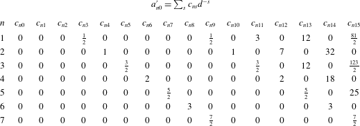
Insertion of (C 5), (C 6) and (C 8) into the boundary conditions (C 7a,b
) and (C 7c,d
) gives a set of equations relating the unknown coefficients
 $A_{nm}^{\prime }$
and
 $a_{nm}^{\prime }$
to one another and the boundary conditions. Solving these equations gives
 $$\begin{eqnarray}\boldsymbol{A}_{m}^{\prime }=(\unicode[STIX]{x1D644}-\unicode[STIX]{x1D648}_{m}\unicode[STIX]{x1D648}_{m})^{-1}\boldsymbol{b}_{m},\quad \boldsymbol{a}_{m}=-\unicode[STIX]{x1D648}_{m}\boldsymbol{A}_{m}^{\prime },\end{eqnarray}$$
where the vectors
 $\boldsymbol{A}_{m}^{\prime }$
and
 $\boldsymbol{a}_{m}^{\prime }$
contain the coefficients
 $(A_{1m}^{\prime },A_{2m}^{\prime },\ldots )$
and
 $(a_{1m}^{\prime },a_{2m}^{\prime },\ldots )$
, while the elements of the square matrix
 $\unicode[STIX]{x1D648}_{m}$
are given by
 $$\begin{eqnarray}\unicode[STIX]{x1D614}_{ns,m}=-\frac{n}{n+1}\frac{1}{d^{s+n+1}}\binom{n+s}{n+m}.\end{eqnarray}$$
The boundary conditions are described by the vectors
 $\boldsymbol{b}_{0}=\{1/2,0,0,\ldots \}$
and
 $\boldsymbol{b}_{1}=\{-1/2,0,0\ldots \}$
.
Inversion of the matrix in (C 9a,b
) is carried out by truncating the infinite series at a finite value
 $n=N$
and solving the resulting equation for
 $A_{nm}^{\prime }$
and
 $a_{nm}^{\prime }$
. This gives asymptotically correct answers, with errors that become negligible if
 $N$
is large enough (Cox, Thamwattana & Hill Reference Cox, Thamwattana and Hill2006). We solved (C 9a,b
) while truncating the series at
 $N=7$
, giving expressions for the microstructure that are accurate to
 $\mathit{O}(d^{-15})$
. Each of the computed coefficients were then expanded as a Taylor series in
 $1/d$
, which are reported to in tables 1, 2, 3 and 4.
Coefficients of the multipole expansion centred at probe I for the perpendicular microstructure
 $f_{1}^{\bot }$
.
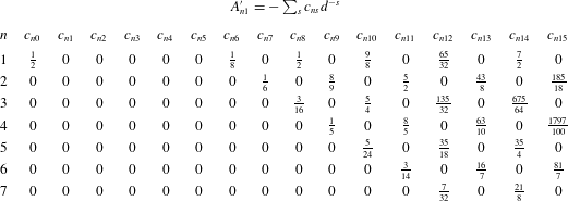
Coefficients of the multipole expansion centred at probe II for the perpendicular microstructure
 $f_{1}^{\bot }$
.
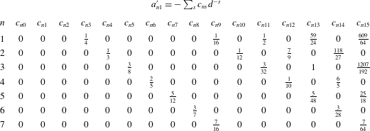
The linear coupling coefficients of
 $\hat{\unicode[STIX]{x1D64D}}_{11}$
and
 $\hat{\unicode[STIX]{x1D64D}}_{12}$
may be determined by substituting the parallel and perpendicular disturbance function (C 5) and (C 6) into the force equation (3.17), giving
 $$\begin{eqnarray}\begin{array}{@{}rcrcrcc@{}}R_{11}^{\Vert }(d)\ & =\ & 6A_{10}^{\prime }(d)-2, & & R_{12}^{\Vert }(d)\ & =\ & -6a_{10}^{\prime }(d),\\ R_{11}^{\bot }(d)\ & =\ & -6A_{11}^{\prime }(d)-2, & & R_{12}^{\bot }(d)\ & =\ & -6a_{11}^{\prime }(d),\end{array}\end{eqnarray}$$
after invoking the boundary conditions (C 7a,b
) and (C 7c,d
). The use of the twin-multipole expansion provides an accurate method for the analytical computation of the scalar couplings between drag force and probe velocity in the linear-response regime for all separations
 $d>2$
.
Analytical results for the scalar couplings, valid for
 $d>2$
, are reported here to
 $\mathit{O}(d^{-15})$
:
 $$\begin{eqnarray}\displaystyle \displaystyle R_{11}^{\Vert } & = & \displaystyle 1+\frac{3}{d^{6}}+\frac{9}{d^{8}}+\frac{18}{d^{10}}+\frac{33}{d^{12}}+\frac{72}{d^{14}}+O\left(\frac{1}{d^{16}}\right),\end{eqnarray}$$
 $$\begin{eqnarray}\displaystyle \displaystyle R_{12}^{\Vert } & = & \displaystyle -\frac{3}{d^{3}}-\frac{3}{d^{9}}-\frac{18}{d^{11}}-\frac{72}{d^{13}}-\frac{243}{d^{15}}+O\left(\frac{1}{d^{17}}\right),\end{eqnarray}$$
 $$\begin{eqnarray}\displaystyle \displaystyle R_{11}^{\bot } & = & \displaystyle 1+\frac{3}{4d^{6}}+\frac{3}{d^{8}}+\frac{27}{4d^{10}}+\frac{195}{16d^{12}}+\frac{21}{d^{14}}+O\left(\frac{1}{d^{16}}\right),\end{eqnarray}$$
 $$\begin{eqnarray}\displaystyle \displaystyle R_{12}^{\bot } & = & \displaystyle \frac{3}{2d^{3}}+\frac{3}{8d^{9}}+\frac{3}{d^{11}}+\frac{59}{4d^{13}}+\frac{1827}{32d^{15}}+O\left(\frac{1}{d^{17}}\right).\end{eqnarray}$$
These results are consistent with the results of Krüger & Rauscher (Reference Krüger and Rauscher2007), who computed the
 $\mathit{O}(Pe)$
non-equilibrium forces between probes in the tandem and side-by-side orientations to
 $\mathit{O}(d^{-3})$
. For separations
 $d<2$
, the coupling coefficients by solving (4.2) numerically through finite-difference methods (cf. appendix E). The resulting coupling coefficients were fit to a fourth-order polynomial in the probe separations distance
 $d$
:
 $$\begin{eqnarray}\displaystyle R_{11}^{\Vert } & = & \displaystyle 0.5773d^{4}-2.7391d^{3}+5.1323d^{2}-4.3946d+2.0324,\end{eqnarray}$$
 $$\begin{eqnarray}\displaystyle R_{12}^{\Vert } & = & \displaystyle -0.5730d^{4}+2.7735d^{3}-5.2177d^{2}+4.4971d-1.5351,\end{eqnarray}$$
 $$\begin{eqnarray}\displaystyle R_{11}^{\bot } & = & \displaystyle -0.1097d^{4}+0.4781d^{3}-0.8554d^{2}+1.1442d+0.1126,\end{eqnarray}$$
 $$\begin{eqnarray}\displaystyle R_{12}^{\bot } & = & \displaystyle -0.1113d^{4}+0.5158d^{3}-0.9442d^{2}+0.9061d-0.1723.\end{eqnarray}$$
Appendix D. Computation of the interactive resistance tensor
$\hat{\unicode[STIX]{x1D64F}}_{1}$

Computation of the third-order tensor
 $\hat{\unicode[STIX]{x1D64F}}_{1}$
coupling the interactive force to weakly nonlinear motion requires computation of the
 $\mathit{O}(Pe^{2})$
disturbance function
 $f_{2}$
. As discussed in § 4.1,
 $f_{2}\sim \hat{\boldsymbol{U}}\hat{\boldsymbol{U}}$
, meaning we may obtain an angular decomposition for
 $f_{2}$
in a manner similar to the decomposition of
 $f_{1}$
:
 $$\begin{eqnarray}f_{2}(\boldsymbol{r}\mid \boldsymbol{d};\unicode[STIX]{x1D6FC})=\cos ^{2}\unicode[STIX]{x1D6FC}f_{2}^{\Vert }(\boldsymbol{r}\mid \boldsymbol{d})+\sin ^{2}\unicode[STIX]{x1D6FC}f_{2}^{\bot }(\boldsymbol{r}\mid \boldsymbol{d})+\sin 2\unicode[STIX]{x1D6FC}f_{2}^{\times }(\boldsymbol{r}\mid \boldsymbol{d}).\end{eqnarray}$$
The resulting disturbance function,
 $f_{2}^{\Vert }$
,
 $f_{2}^{\bot }$
, and
 $f_{2}^{\times }$
, are associated with angular variation in the structure arising from motion parallel, perpendicular and diagonal to the probe line of centres, respectively, and may be directly related to the scalar couplings
 $T^{\Vert }$
,
 $T^{\bot }$
, and
 $T^{\times }$
.
Computation of the third-order coupling tensor
 $\hat{\unicode[STIX]{x1D64F}}_{1}$
could proceed as before by obtaining the twin-multipole expansion of
 $f_{2}$
. However, this method proves to be algebraically intractable. To circumvent this issue, we developed a method based on Green’s second identity that allows for the computation of
 $\hat{\unicode[STIX]{x1D64F}}_{1}$
without computing
 $f_{2}$
. The
 $\mathit{O}(Pe^{2})$
disturbance is divided into its homogenous and particular solution:
 $f_{2}=f_{2}^{h}+f_{2}^{p}$
. The homogenous solution
 $(f_{2}^{h})$
is a harmonic function, and the particular solution is given by
 $f_{2}^{p}=-\boldsymbol{r}\boldsymbol{\cdot }\hat{\boldsymbol{U}}f_{1}/2$
, where
 $\boldsymbol{r}$
is the position vector centred at probe I. Substituting this expression for
 $f_{2}$
into integral for the osmotic force (cf. (3.17)) and using the definition for
 $\hat{\unicode[STIX]{x1D64F}}_{1}$
then gives
 $$\begin{eqnarray}\hat{\unicode[STIX]{x1D64F}}_{1}\boldsymbol{ : }\hat{\boldsymbol{U}}\hat{\boldsymbol{U}}=\frac{3}{2\unicode[STIX]{x03C0}}\int \left(f_{2}^{h}(\boldsymbol{r}\mid \boldsymbol{d};\unicode[STIX]{x1D6FC})-\frac{1}{2}\boldsymbol{r}\boldsymbol{\cdot }\hat{\boldsymbol{U}}f_{1}(\boldsymbol{r}\mid \boldsymbol{d};\unicode[STIX]{x1D6FC})\right)\boldsymbol{n}_{1}\,\text{d}S_{\text{I}}.\end{eqnarray}$$
The dependence of (D 2) on
 $f_{2}^{h}$
may be removed by relating it to the
 $\mathit{O}(Pe)$
microstructure through Green’s second identity, which holds for any two harmonic functions:
 $$\begin{eqnarray}\int f_{2}^{h}\boldsymbol{n}\boldsymbol{\cdot }\unicode[STIX]{x1D735}\tilde{f}_{1(1)}\,\text{d}S=\int \tilde{f}_{1(1)}\boldsymbol{n}\boldsymbol{\cdot }\unicode[STIX]{x1D735}f_{2}^{h}\,\text{d}S.\end{eqnarray}$$
Here, the surface integral is evaluated over both
 $S_{\text{I}}$
and
 $S_{\text{II}}$
. The tilde in
 $\tilde{f}_{1(1)}$
emphasizes that this expression holds true for all values of
 $\tilde{f}_{1(1)}$
, meaning the velocity vector associated with
 $\tilde{f}_{1(1)}$
need not be oriented in the same direction as that associated with
 $f_{2}^{h}$
. From (C 4a
) and (C 4b
), it can be seen that
 $\boldsymbol{n}\boldsymbol{\cdot }\unicode[STIX]{x1D735}\tilde{f}_{1(1)}=-\boldsymbol{n}\boldsymbol{\cdot }\tilde{\boldsymbol{U}}$
on
 $S_{\text{I}}$
and
 $\boldsymbol{n}\boldsymbol{\cdot }\unicode[STIX]{x1D735}f_{1(1)}=0$
on
 $S_{\text{II}}$
, where
 $\tilde{\boldsymbol{U}}$
is the dimensionless probe velocity associated with
 $\tilde{f}_{1(1)}$
. Substituting these boundary conditions into (D 3) gives
 $$\begin{eqnarray}-\tilde{\boldsymbol{U}}\boldsymbol{\cdot }\int f_{2}^{h}\boldsymbol{n}_{1}\,\text{d}S_{\text{II}}=\int \tilde{f}_{1(1)}\boldsymbol{n}_{1}\boldsymbol{\cdot }\unicode[STIX]{x1D735}f_{2}^{h}\,\text{d}S_{\text{I}}+\int \tilde{f}_{1(1)}\boldsymbol{n}_{2}\boldsymbol{\cdot }\unicode[STIX]{x1D735}f_{2}^{h}\,\text{d}S_{\text{II}}.\end{eqnarray}$$
The resulting expression may be substituted into (D 2), giving
 $$\begin{eqnarray}\displaystyle \tilde{\boldsymbol{U}}\boldsymbol{\cdot }\hat{\unicode[STIX]{x1D64F}}_{1}\boldsymbol{ : }\hat{\boldsymbol{U}}\hat{\boldsymbol{U}} & = & \displaystyle -\frac{3}{4\unicode[STIX]{x03C0}}\int \boldsymbol{n}_{1}\boldsymbol{\cdot }\hat{\boldsymbol{U}}f_{1}\tilde{f}_{1(1)}+\boldsymbol{n}_{1}\boldsymbol{n}_{1}\boldsymbol{ : }\hat{\boldsymbol{U}}\hat{\boldsymbol{U}}\tilde{f}_{1(1)}-\boldsymbol{n}_{1}\boldsymbol{n}_{1}\boldsymbol{ : }\hat{\boldsymbol{U}}\tilde{\boldsymbol{U}}f_{1}\,\text{d}S_{\text{I}}\nonumber\\ \displaystyle & & \displaystyle -\,\frac{3}{4\unicode[STIX]{x03C0}}\int \boldsymbol{n}_{2}\boldsymbol{\cdot }\hat{\boldsymbol{U}}f_{1}\tilde{f}_{1(1)}+\boldsymbol{n}_{2}(\boldsymbol{n}_{2}+\boldsymbol{d})\boldsymbol{ : }\hat{\boldsymbol{U}}\hat{\boldsymbol{U}}\tilde{f}_{1(1)}\,\text{d}S_{\text{II}}.\end{eqnarray}$$
Here, we have simplified the right-hand side of (D 4) using (4.3b
), and have used
 $\boldsymbol{r}|_{S_{\text{II}}}=\boldsymbol{n}_{2}+\boldsymbol{d}$
. The resulting expression depends only on the
 $\mathit{O}(Pe)$
microstructure functions
 $f_{1}$
and
 $\tilde{f}_{1(1)}$
. From (C 2), it is seen that
 $f_{1}$
is obtained from a linear combination of the functions
 $f_{1}^{\Vert }=f_{1(1)}^{\Vert }+f_{1(2)}^{\Vert }$
and
 $f_{1}^{\bot }=f_{1(1)}^{\bot }+f_{1(2)}^{\bot }$
. Using the results of appendix C, it can be shown that
 $$\begin{eqnarray}\displaystyle & \displaystyle f_{1}^{\Vert }=\mathop{\sum }_{n=1}^{\infty }A_{n0}\frac{1}{r^{n+1}}P_{n}(\cos \unicode[STIX]{x1D703})+a_{n0}\frac{1}{{r^{\prime }}^{n+1}}P_{n}(\cos \unicode[STIX]{x1D703}^{\prime }), & \displaystyle\end{eqnarray}$$
 $$\begin{eqnarray}\displaystyle & \displaystyle f_{1}^{\bot }=\mathop{\sum }_{n=1}^{\infty }\left[A_{n1}\frac{1}{r^{n+1}}P_{n}^{1}(\cos \unicode[STIX]{x1D703})+a_{n1}\frac{1}{{r^{\prime }}^{n+1}}P_{n}^{1}(\cos \unicode[STIX]{x1D703}^{\prime })\right]\cos (\unicode[STIX]{x1D719}), & \displaystyle\end{eqnarray}$$
where the coefficients
 $A_{nm}$
and
 $a_{nm}$
may be obtained from the symmetry relations
 $$\begin{eqnarray}\displaystyle A_{nm}=A_{nm}^{\prime }-(-1)^{m}a_{nm}^{\prime },\quad a_{nm}=a_{nm}^{\prime }-(-1)^{m}A_{nm}^{\prime }. & & \displaystyle\end{eqnarray}$$
Thus, computation of
 $f_{2}$
is not necessary to compute
 $\hat{\unicode[STIX]{x1D64F}}_{1}$
; all that is needed are the
 $\mathit{O}(Pe)$
functions computed in appendix C.
The individual scalar components of
 $\hat{\unicode[STIX]{x1D64F}}_{1}$
may be computed through appropriate choices of
 $\hat{\boldsymbol{U}}$
and
 $\tilde{\boldsymbol{U}}$
. In (D 5),
 $\tilde{\boldsymbol{U}}$
gives the projection of the weakly nonlinear interactive force in the
 $\tilde{\boldsymbol{U}}$
direction. Thus, setting
 $\tilde{\boldsymbol{U}}=\boldsymbol{e}_{z}$
gives the parallel interactive force, while
 $\tilde{\boldsymbol{U}}=\boldsymbol{e}_{x}$
gives the perpendicular interactive force. The coupling
 $T^{\Vert }$
gives the relation between the parallel interactive force and motion along the probes line of centres. Thus, it may be found by choosing
 $\tilde{f}_{1(1)}$
and
 $f_{1}$
such that
 $\tilde{\boldsymbol{U}}=\hat{\boldsymbol{U}}=\boldsymbol{e}_{z}$
:
 $$\begin{eqnarray}\displaystyle T^{\Vert } & = & \displaystyle -\frac{3}{4\unicode[STIX]{x03C0}}\int \boldsymbol{n}_{1}\boldsymbol{\cdot }\boldsymbol{e}_{z}f_{1(1)}^{\Vert }f_{1(1)}^{\Vert }\,\text{d}S_{\text{I}}\nonumber\\ \displaystyle & & \displaystyle -\,\frac{3}{4\unicode[STIX]{x03C0}}\int \boldsymbol{n}_{2}\boldsymbol{\cdot }\boldsymbol{e}_{z}f_{1(1)}^{\Vert }f_{1(1)}^{\Vert }+\boldsymbol{n}_{2}(2\boldsymbol{n}_{2}+\boldsymbol{d})\boldsymbol{ : }\boldsymbol{e}_{z}\boldsymbol{e}_{z}f_{1(1)}^{\Vert }\,\text{d}S_{\text{II}},\end{eqnarray}$$
where (D 8a,b
) has been used to simplify. Keeping
 $\tilde{f}_{1(1)}$
the same and choosing
 $f_{1}$
such that
 $\hat{\boldsymbol{U}}=\boldsymbol{e}_{x}$
gives
 $$\begin{eqnarray}\displaystyle T^{\bot } & = & \displaystyle -\frac{3}{4\unicode[STIX]{x03C0}}\int \boldsymbol{n}_{1}\boldsymbol{\cdot }\boldsymbol{e}_{x}f_{1}^{\bot }f_{1(1)}^{\Vert }+\boldsymbol{n}_{1}\boldsymbol{n}_{1}\boldsymbol{ : }\boldsymbol{e}_{x}\boldsymbol{e}_{x}f_{1(1)}^{\Vert }-\boldsymbol{n}_{1}\boldsymbol{n}_{1}\boldsymbol{ : }\boldsymbol{e}_{x}\boldsymbol{e}_{z}f_{1}^{\bot }\,\text{d}S_{\text{I}}\nonumber\\ \displaystyle & & \displaystyle -\,\frac{3}{4\unicode[STIX]{x03C0}}\int \boldsymbol{n}_{2}\boldsymbol{\cdot }\boldsymbol{e}_{x}f_{1}^{\bot }f_{1(1)}^{\Vert }+\boldsymbol{n}_{2}\boldsymbol{n}_{2}\boldsymbol{ : }\boldsymbol{e}_{x}\boldsymbol{e}_{x}f_{1(1)}^{\Vert }\,\text{d}S_{\text{II}},\end{eqnarray}$$
where the results have again been simplified. The third coupling can be found by setting
 $\tilde{\boldsymbol{U}}$
to
 $\boldsymbol{e}_{x}$
and
 $\hat{\boldsymbol{U}}$
to
 $(\boldsymbol{e}_{x}+\boldsymbol{e}_{z})/\sqrt{2}$
, giving
 $$\begin{eqnarray}\displaystyle T^{\times } & = & \displaystyle -\frac{3}{8\unicode[STIX]{x03C0}}\int \boldsymbol{n}_{1}\boldsymbol{\cdot }(\boldsymbol{e}_{z}f_{1(1)}^{\bot }f_{1(1)}^{\bot }+\boldsymbol{e}_{x}f_{1}^{\Vert }f_{1(1)}^{\bot })+\boldsymbol{e}_{x}\boldsymbol{\cdot }\boldsymbol{n}_{1}\boldsymbol{n}_{1}\boldsymbol{\cdot }(\boldsymbol{e}_{z}f_{1(1)}^{\bot }-\boldsymbol{e}_{x}f_{1}^{\Vert })\,\text{d}S_{\text{I}}\nonumber\\ \displaystyle & & \displaystyle -\,\frac{3}{8\unicode[STIX]{x03C0}}\int \boldsymbol{n}_{2}\boldsymbol{\cdot }(\boldsymbol{e}_{z}f_{1(1)}^{\bot }f_{1(1)}^{\bot }+\boldsymbol{e}_{x}f_{1}^{\Vert }f_{1(1)}^{\bot })+\boldsymbol{n}_{2}(3\boldsymbol{n}_{2}+\boldsymbol{d})\boldsymbol{ : }\boldsymbol{e}_{z}\boldsymbol{e}_{x}f_{1(1)}^{\bot }\,\text{d}S_{\text{II}}.\end{eqnarray}$$
Analytical expressions, valid for
 $d>2$
, are reported here to
 $\mathit{O}(d^{-15})$
:
 $$\begin{eqnarray}\displaystyle T^{\Vert } & = & \displaystyle \frac{1}{2d^{2}}-\frac{2}{d^{4}}+\frac{1}{d^{5}}+\frac{1}{d^{7}}+\frac{1}{2d^{8}}-\frac{1}{d^{9}}+\frac{2}{d^{10}}-\frac{5}{d^{11}}+\frac{5}{d^{12}}-\frac{8}{d^{13}}+\frac{15}{2d^{14}}\nonumber\\ \displaystyle & & \displaystyle +\,\frac{2}{d^{15}}+O\left(\frac{1}{d^{16}}\right),\end{eqnarray}$$
 $$\begin{eqnarray}\displaystyle T^{\bot } & = & \displaystyle -\frac{3}{4d^{2}}+\frac{1}{d^{4}}-\frac{9}{8d^{5}}-\frac{1}{d^{7}}-\frac{21}{16d^{8}}+\frac{25}{24d^{9}}-\frac{5}{d^{10}}+\frac{147}{32d^{11}}-\frac{295}{24d^{12}}+\frac{21}{4d^{13}}\nonumber\\ \displaystyle & & \displaystyle -\,\frac{13349}{576d^{14}}-\frac{1261}{96d^{15}}+O\left(\frac{1}{d^{16}}\right),\end{eqnarray}$$
 $$\begin{eqnarray}\displaystyle T^{\times } & = & \displaystyle -\frac{1}{2d^{2}}+\frac{1}{d^{4}}-\frac{1}{16d^{5}}+\frac{1}{16d^{8}}-\frac{59}{48d^{9}}-\frac{301}{64d^{11}}-\frac{5}{24d^{12}}-\frac{95}{8d^{13}}\nonumber\\ \displaystyle & & \displaystyle +\,\frac{821}{576d^{14}}+O\left(\frac{1}{d^{16}}\right).\end{eqnarray}$$
For separations
 $d<2$
, the coupling coefficients by solving (4.3) numerically through finite-difference methods (cf. appendix E). The resulting coupling coefficients were again fit to a fourth-order polynomial in the probe separations distance
 $d$
:
 $$\begin{eqnarray}\displaystyle T^{\Vert } & = & \displaystyle -0.0692d^{4}+0.3762d^{3}-0.8354d^{2}+0.7331d-0.0039,\end{eqnarray}$$
 $$\begin{eqnarray}\displaystyle T^{\bot } & = & \displaystyle -0.0508d^{4}+0.1919d^{3}-0.5372d^{2}+0.5958d+0.0483,\end{eqnarray}$$
 $$\begin{eqnarray}\displaystyle T^{\times } & = & \displaystyle 0.0393d^{4}-0.1845d^{3}+0.3123d^{2}-0.2813d+0.0881.\end{eqnarray}$$
Appendix E. Numerical solution for arbitrary forcing strength
The analytical perturbation methods employed in the preceding section are only valid for
 $Pe\ll 1$
and
 $d>2$
. For
 $Pe\gtrsim \mathit{O}(1)$
and for separations
 $d<2$
, numerical methods are required. The Cartesian coordinate system describing probe geometry (cf. figure 3) is transformed into a curvilinear coordinate system where the no-flux surfaces of the probes coincide with coordinate isosurfaces. The nature of the required coordinate system depends crucially on the probe separation distance
 $d$
. When
 $d<2$
, bath particles cannot fit directly between the two probes, and their excluded-volume surfaces
 $S_{\text{I}}$
and
 $S_{\text{II}}$
overlap, forming a dumbbell-like shape. For
 $d>2$
, bath particles may freely move between the probes, and the excluded-volume surfaces of the probes take the form of non-overlapping spheres. This difference in geometry necessitates the use of two different coordinate systems. The appropriate coordinate systems for the solution of the Smoluchowski equation are then toroidal coordinates for
 $d<2$
, and bispherical coordinates for
 $d>2$
. Khair & Brady (Reference Khair and Brady2007) used these coordinate systems to compute the forces exerted on two probes moving in the tandem orientation. Their numerical method relied on mapping the advection-diffusion equation to the Helmholtz equation. As this method leads to numerical difficulties for large values of
 $Pe$
, we use an alternative formulation.
The formulation of the Smoluchowski equation in toroidal and bispherical coordinates is presented in the succeeding sections. For ease of readability, we will define three scalar functions that appear often in the coordinate systems:
 $$\begin{eqnarray}\displaystyle R=\cosh \unicode[STIX]{x1D707}-\cos \unicode[STIX]{x1D702},\quad A=1-\cosh \unicode[STIX]{x1D707}\cos \unicode[STIX]{x1D702},\quad B=\sinh \unicode[STIX]{x1D707}\sin \unicode[STIX]{x1D702}. & & \displaystyle\end{eqnarray}$$
E.1 Toroidal coordinates
$d<2$

The toroidal coordinate system is defined by the relations
 $$\begin{eqnarray}\displaystyle x=c\frac{\sinh \unicode[STIX]{x1D707}\cos \unicode[STIX]{x1D719}}{\cosh \unicode[STIX]{x1D707}-\cos \unicode[STIX]{x1D702}},\quad y=c\frac{\sinh \unicode[STIX]{x1D707}\sin \unicode[STIX]{x1D719}}{\cosh \unicode[STIX]{x1D707}-\cos \unicode[STIX]{x1D702}},\quad z=c\frac{\sin \unicode[STIX]{x1D702}}{\cosh \unicode[STIX]{x1D707}-\cos \unicode[STIX]{x1D702}}, & & \displaystyle\end{eqnarray}$$
where
 $c$
is a constant scale factor setting the geometry of the coordinate systems, and the three coordinates span
 $0\leqslant \unicode[STIX]{x1D707}<\infty$
,
 $-\unicode[STIX]{x03C0}\leqslant \unicode[STIX]{x1D702}\leqslant \unicode[STIX]{x03C0}$
and
 $0\leqslant \unicode[STIX]{x1D719}\leqslant 2\unicode[STIX]{x03C0}$
. Surfaces of constant
 $\unicode[STIX]{x1D702}$
are overlapping spheres given by
 $x^{2}+y^{2}+(z-ac\cot \unicode[STIX]{x1D702})^{2}=a^{2}c^{2}/\sin ^{2}\unicode[STIX]{x1D702}$
, meaning the excluded-volume surfaces of the probes
 $S_{\text{I}}$
and
 $S_{\text{II}}$
can be described by the isosurfaces
 $\unicode[STIX]{x1D702}=\pm \unicode[STIX]{x1D702}_{0}$
. As
 $S_{\text{I}}$
and
 $S_{\text{II}}$
are located at
 $z=\pm d/2$
and have a radius of unity, the coordinate isosurfaces are given by
 $\unicode[STIX]{x1D702}_{0}=\cos ^{-1}(d/2)$
with the scale factor
 $c=\sqrt{4-d^{2}}/2$
.
We make the substitution
 $f=c\sqrt{R}h$
in (3.10a
), which has the advantage of automatically satisfying the far-field boundary conditions (3.10c
), as
 $R\rightarrow 0$
as
 $r\rightarrow \infty$
. With this substitution, equations (3.10a
) and (3.10b
) become
 $$\begin{eqnarray}\displaystyle & & \displaystyle \frac{\unicode[STIX]{x2202}^{2}h}{\unicode[STIX]{x2202}\unicode[STIX]{x1D707}^{2}}+\frac{\unicode[STIX]{x2202}^{2}h}{\unicode[STIX]{x2202}\unicode[STIX]{x1D702}^{2}}+\coth \unicode[STIX]{x1D707}\frac{\unicode[STIX]{x2202}h}{\unicode[STIX]{x2202}\unicode[STIX]{x1D702}}+\text{csch}^{2}\unicode[STIX]{x1D707}\frac{\unicode[STIX]{x2202}^{2}h}{\unicode[STIX]{x2202}\unicode[STIX]{x1D719}^{2}}+\frac{1}{4}h\nonumber\\ \displaystyle & & \displaystyle \quad +\,\frac{cPe\sin \unicode[STIX]{x1D6FC}\cos \unicode[STIX]{x1D719}}{R^{2}}\left[-B\frac{\unicode[STIX]{x2202}g}{\unicode[STIX]{x2202}\unicode[STIX]{x1D702}}+A\frac{\unicode[STIX]{x2202}g}{\unicode[STIX]{x2202}\unicode[STIX]{x1D707}}-R\text{csch}\unicode[STIX]{x1D707}\frac{\unicode[STIX]{x2202}h}{\unicode[STIX]{x2202}\unicode[STIX]{x1D719}}-\frac{1}{2}\sinh \unicode[STIX]{x1D707}\cos \unicode[STIX]{x1D702}h\right]\nonumber\\ \displaystyle & & \displaystyle \quad +\,\frac{cPe\cos \unicode[STIX]{x1D6FC}}{R^{2}}\left[-A\frac{\unicode[STIX]{x2202}g}{\unicode[STIX]{x2202}\unicode[STIX]{x1D702}}-B\frac{\unicode[STIX]{x2202}g}{\unicode[STIX]{x2202}\unicode[STIX]{x1D707}}-\frac{1}{2}\cosh \unicode[STIX]{x1D707}\sin \unicode[STIX]{x1D702}h\right]=0,\end{eqnarray}$$
 $$\begin{eqnarray}\displaystyle \left.\left(\frac{\unicode[STIX]{x2202}h}{\unicode[STIX]{x2202}\unicode[STIX]{x1D702}}+\frac{1}{2}\frac{\sin \unicode[STIX]{x1D702}}{R}h\right)\right|_{\unicode[STIX]{x1D702}=\pm \unicode[STIX]{x1D702}_{0}}=\left(\frac{A\cos \unicode[STIX]{x1D6FC}}{R^{5/2}}+\frac{B\cos \unicode[STIX]{x1D719}\sin \unicode[STIX]{x1D6FC}}{R^{5/2}}\right)(1+cPe\sqrt{R}h)|_{\unicode[STIX]{x1D702}=\pm \unicode[STIX]{x1D702}_{0}}. & & \displaystyle\end{eqnarray}$$
The equations are discretized via a second-order finite-difference scheme, and the resulting equations are solved iteratively using the MATLAB program gmres with incomplete
 $LU$
prefactorization. The
 $\unicode[STIX]{x1D707}$
coordinate, which lies in
 $\unicode[STIX]{x1D707}\in [0,\infty )$
is restricted to
 $\unicode[STIX]{x1D707}\in [0,\unicode[STIX]{x1D707}_{\infty }]$
, where
 $\unicode[STIX]{x1D707}_{\infty }$
is chosen such that the numerical results are equivalent to choosing
 $\unicode[STIX]{x1D707}=\infty$
. Typically,
 $\unicode[STIX]{x1D707}_{\infty }=10$
is sufficient.
For
 $Pe\ll 1$
, a grid that is evenly spaced in
 $\unicode[STIX]{x1D702}$
,
 $\unicode[STIX]{x1D707}$
and
 $\unicode[STIX]{x1D719}$
is sufficient to ensure accurate numerical solutions of the Smoluchowski equation. However, when
 $Pe\gg 1$
, the numerical method must both resolve an
 $\mathit{O}(Pe^{-1})$
thin boundary layer in the upstream region and an
 $\mathit{O}(Pe)$
long trailing wake. To reduce the number of grid points necessary, coordinate transformations are introduced. When the probes are near the side-by-side orientation
 $(\unicode[STIX]{x1D6FC}=\unicode[STIX]{x03C0}/2)$
, the transforms of Khair & Brady (Reference Khair and Brady2007) are used:
 $$\begin{eqnarray}\unicode[STIX]{x1D702}=\unicode[STIX]{x1D702}_{0}\coth a\tanh \left(\frac{a\unicode[STIX]{x1D706}}{2}\right)\end{eqnarray}$$
and
 $$\begin{eqnarray}\unicode[STIX]{x1D707}=\exp (\log (\unicode[STIX]{x1D707}_{\infty }+1)\unicode[STIX]{x1D709})-1,\end{eqnarray}$$
where
 $-1\leqslant \unicode[STIX]{x1D706}\leqslant 1$
,
 $0\leqslant \unicode[STIX]{x1D709}\leqslant 1$
and
 $a$
is an adjustable parameter. These transformations increase the number of grid points in the boundary layer and increase the density of grid points near the point where the excluded-volume surfaces of the probes overlap. Increasing
 $a$
increases the density of grid points in the boundary layer. When the probes are near the tandem orientation (
 $\unicode[STIX]{x1D6FC}=0$
), it is desirable to increase the number of grid points near the
 $z$
axis to resolve interactions between the wake of the leading probe and the no-flux surface of the trailing probe. To this end, the transform
 $$\begin{eqnarray}\unicode[STIX]{x1D707}=\unicode[STIX]{x1D707}_{\infty }\frac{\sinh (n\unicode[STIX]{x1D709})}{\sinh n}\end{eqnarray}$$
is employed, with
 $n$
as an adjustable parameter. Increasing the value of
 $n$
increases the number of grid points near the wake region.
E.2 Bispherical coordinates
$d>2$

The bispherical coordinate systems is defined as
 $$\begin{eqnarray}x=c\frac{\sin \unicode[STIX]{x1D702}\cos \unicode[STIX]{x1D719}}{\cosh \unicode[STIX]{x1D707}-\cos \unicode[STIX]{x1D702}},\quad y=c\frac{\sin \unicode[STIX]{x1D702}\sin \unicode[STIX]{x1D719}}{\cosh \unicode[STIX]{x1D707}-\cos \unicode[STIX]{x1D702}},\quad z=c\frac{\sinh \unicode[STIX]{x1D707}}{\cosh \unicode[STIX]{x1D707}-\cos \unicode[STIX]{x1D702}},\end{eqnarray}$$
where
 $c$
is a scale factor and the three coordinates span
 $-\infty <\unicode[STIX]{x1D707}<\infty$
,
 $0\leqslant \unicode[STIX]{x1D702}\leqslant \unicode[STIX]{x03C0}$
and
 $0\leqslant \unicode[STIX]{x1D719}\leqslant 2\unicode[STIX]{x03C0}$
. Surfaces of constant
 $\unicode[STIX]{x1D707}$
are spheres given by
 $x^{2}+y^{2}+(z-c\coth \unicode[STIX]{x1D707})^{2}=c^{2}/\sinh ^{2}\unicode[STIX]{x1D707}$
. Thus, the excluded-volume surfaces of the probes are given by
 $\unicode[STIX]{x1D707}=\pm \unicode[STIX]{x1D707}_{0}$
, where
 $\unicode[STIX]{x1D707}=\cosh ^{-1}(d/2)$
and the scale factor is
 $c=\sqrt{d^{2}-4}/2$
.
We again make the substitution
 $f=c\sqrt{R}h$
and (3.10a
) and (3.10b
) become
 $$\begin{eqnarray}\displaystyle & & \displaystyle \frac{\unicode[STIX]{x2202}^{2}h}{\unicode[STIX]{x2202}\unicode[STIX]{x1D707}^{2}}+\frac{\unicode[STIX]{x2202}^{2}h}{\unicode[STIX]{x2202}\unicode[STIX]{x1D702}^{2}}+\cot \unicode[STIX]{x1D702}\frac{\unicode[STIX]{x2202}h}{\unicode[STIX]{x2202}\unicode[STIX]{x1D707}}+\csc ^{2}\unicode[STIX]{x1D702}\frac{\unicode[STIX]{x2202}^{2}h}{\unicode[STIX]{x2202}\unicode[STIX]{x1D719}^{2}}-\frac{1}{4}h\nonumber\\ \displaystyle & & \displaystyle \quad +\,\frac{Pe\sin \unicode[STIX]{x1D6FC}\cos \unicode[STIX]{x1D719}}{R^{2}}\left[-B\frac{\unicode[STIX]{x2202}g}{\unicode[STIX]{x2202}\unicode[STIX]{x1D707}}-A\frac{\unicode[STIX]{x2202}g}{\unicode[STIX]{x2202}\unicode[STIX]{x1D702}}-R\csc \unicode[STIX]{x1D702}\frac{\unicode[STIX]{x2202}h}{\unicode[STIX]{x2202}\unicode[STIX]{x1D719}}-\frac{1}{2}\cosh \unicode[STIX]{x1D707}\sin \unicode[STIX]{x1D702}h\right]\nonumber\\ \displaystyle & & \displaystyle \quad +\,\frac{cPe\cos \unicode[STIX]{x1D6FC}}{R^{2}}\left[A\frac{\unicode[STIX]{x2202}g}{\unicode[STIX]{x2202}\unicode[STIX]{x1D707}}-B\frac{\unicode[STIX]{x2202}g}{\unicode[STIX]{x2202}\unicode[STIX]{x1D702}}-\frac{1}{2}\sinh \unicode[STIX]{x1D707}\cos \unicode[STIX]{x1D702}h\right]=0,\end{eqnarray}$$
 $$\begin{eqnarray}\left.\left(\frac{\unicode[STIX]{x2202}h}{\unicode[STIX]{x2202}\unicode[STIX]{x1D707}}+\frac{1}{2}\frac{\sinh \unicode[STIX]{x1D707}}{R}h\right)\right|_{\unicode[STIX]{x1D707}=\pm \unicode[STIX]{x1D707}_{0}}=\left(-\frac{A\cos \unicode[STIX]{x1D6FC}}{R^{5/2}}+\frac{B\cos \unicode[STIX]{x1D719}\sin \unicode[STIX]{x1D6FC}}{R^{5/2}}\right)(1+cPe\sqrt{R}h)|_{\unicode[STIX]{x1D707}=\pm \unicode[STIX]{x1D707}_{0}}.\end{eqnarray}$$
In bispherical coordinates, equation (E 5) is used to transform the
 $\unicode[STIX]{x1D707}$
coordinate, increasing the number of grid points in the boundary layer. For probes near the side-by-side orientation, a grid that is equally spaced in
 $\unicode[STIX]{x1D702}$
is sufficient. However, for probes near the tandem orientation, an increase in grid point density in the wake is obtained by using (E 7) to transform
 $\unicode[STIX]{x1D702}$
.