1 Introduction
Marangoni stresses due to the variation in surface tension at the interface separating two immiscible fluids play a vital role in many technological applications. The surface tension gradient at the interface can occur due to the variation in either temperature or concentration of surfactants. A characteristic problem of this nature is the thermocapillary migration of a drop/bubble. Extensive reviews on this subject can be found in Subramanian (Reference Subramanian1992) and Subramanian, Balasubramaniam & Wozniak (Reference Subramanian, Balasubramaniam, Wozniak and Monti2002). In the present work, we numerically investigate the thermocapillary migration of a bubble inside a three-dimensional channel filled with a so-called ‘self-rewetting’ fluid that exhibits a non-monotonic dependence of the surface tension on temperature. This behaviour is in contrast with that of common fluids (hereafter termed ‘linear’ fluids), such as water and various oils, whose interfacial tension with air typically decreases almost linearly with increasing temperature. A typical example of self-rewetting fluids are non-azeotropic, high-carbon alcohol solutions, which have quasi-parabolic surface tension–temperature curves with well-defined minima; increasing alcohol concentration increases the parabolicity of these curves (Vochten & Petre Reference Vochten and Petre1973; Petre & Azouni Reference Petre and Azouni1984; Limbourgfontaine, Petre & Legros Reference Limbourgfontaine, Petre and Legros1986; Villers & Platten Reference Villers and Platten1988; Savino, Cecere & Paola Reference Savino, Cecere and Paola2009; Savino et al. Reference Savino, Cecere, Vaerenbergh, Abe, Pizzirusso, Tzevelecos, Mojahed and Galand2013). This unusual surface tension dependence on temperature was first observed by Vochten & Petre (Reference Vochten and Petre1973), and such fluids were later termed self-rewetting by Abe, Iwasaki & Tanaka (Reference Abe, Iwasaki and Tanaka2004). It has been shown that the properties of these fluids can be exploited to accomplish substantially higher critical heat fluxes in heat pipes compared to water (McGillis & Carey Reference McGillis and Carey1996; Ahmed & Carey Reference Ahmed and Carey1999; Suzuki, Nakano & Itoh Reference Suzuki, Nakano and Itoh2005) or may even give rise to some very interesting phenomena, such as thermally induced ‘superspreading’ behaviour of a droplet on a surface (Karapetsas et al. Reference Karapetsas, Sahu, Sefiane and Matar2014).
The thermal migration of bubbles in a linear viscous fluid heated from below was first reported in the pioneering work of Young, Goldstein & Block (Reference Young, Goldstein and Block1959), who experimentally demonstrated that, due to the Marangoni stresses induced by the temperature gradient, small bubbles move in the downward direction, whereas larger bubbles move in the upward direction. In the latter case, the buoyancy overcomes the effect of thermocapillarity. Assuming a spherical-shaped bubble and creeping flow conditions, they also derived an analytical expression for the terminal velocity of the bubble. Later, in the context of microgravity applications, Balasubramaniam & Chai (Reference Balasubramaniam and Chai1987) neglected buoyancy and extended the analytical solution to bubbles with small deformation from a spherical shape. By conducting an asymptotic analysis in the limit of large Reynolds and Marangoni numbers, Balasubramaniam (Reference Balasubramaniam1998) reported that the steady migration velocity is a linear combination of the velocity for purely thermocapillary motion and the buoyancy-driven rising velocity. Later, Zhang, Subramanian & Balasubramaniam (Reference Zhang, Subramanian and Balasubramaniam2001) performed a theoretical analysis and showed that for small Marangoni numbers the inclusion of inertia is crucial in the development of an asymptotic solution for the temperature field. Recently, by conducting numerical simulations of a droplet inside a rectangular box, Brady, Herrmann & Lopez (Reference Brady, Herrmann and Lopez2011) showed that for low Marangoni numbers a drop rapidly reached a quasi-steady state, but for high Marangoni numbers the initial conditions affect the behaviour of the droplet significantly. The thermocapillary migration of a bubble for high Marangoni numbers was also investigated by Liu, Zhang & Valocchi (Reference Liu, Zhang and Valocchi2012). They showed that the terminal velocity of the bubble decreases with increasing Marangoni number.
Merritt, Morton & Subramanian (Reference Merritt, Morton and Subramanian1993) studied the migration of bubbles in the presence of buoyancy and thermocapillarity via direct numerical simulations. Since then, several kinds of numerical methods – ranging from boundary-fitted grids (Chen & Lee Reference Chen and Lee1992; Welch Reference Welch1998), to the level-set method (Haj-Hariri, Shi & Borhan Reference Haj-Hariri, Shi and Borhan1997; Zhao et al. Reference Zhao, Li, Li and Li2010), the volume-of-fluid (VoF) method (Ma & Bothe Reference Ma and Bothe2011; Tripathi et al. Reference Tripathi, Sahu, Karapetsas and Matar2015b ), diffuse-interface methods (Borcia & Bestehorn Reference Borcia and Bestehorn2007) and hybrid schemes of the lattice Boltzmann and the finite difference method (Liu et al. Reference Liu, Valocchi, Zhang and Kang2013) – have been proposed in order to obtain the surface deformation accurately. Some of the main findings from these studies are highlighted below. Chen & Lee (Reference Chen and Lee1992) and Haj-Hariri et al. (Reference Haj-Hariri, Shi and Borhan1997) showed that the deformation considerably reduces the terminal velocity of both gas bubbles and liquid drops. Welch (Reference Welch1998) demonstrated that for higher capillary numbers bubble deformation becomes important and the bubble continues to deform at later times, failing to reach a steady state. Herrmann et al. (Reference Herrmann, Lopez, Brady and Raessi2008a ) and Wu & Hu (Reference Wu and Hu2012, Reference Wu and Hu2013) also reached the same conclusion for the case of large Marangoni numbers. Keh, Chen & Chen (Reference Keh, Chen and Chen2002) numerically studied the motion of a spherical drop between two parallel plane walls and found that the droplet migration speed can be controlled by varying the thermal conductivity of the droplet and changing the imposed boundary conditions at the wall. Chen, Dagan & Maldarelli (Reference Chen, Dagan and Maldarelli1991) found that inside an insulated tube with an imposed axial temperature gradient, which in turn develops the hydrodynamic retarding forces, the thermocapillary migration velocity of a spherical drop is always less than that in an infinite medium. This work was extended by Mahesri, Haj-Hariri & Borhan (Reference Mahesri, Haj-Hariri and Borhan2014) to take into account the effect of interfacial deformation. All these studies considered the migration of bubbles and drops in linear fluids.
Tripathi et al. (Reference Tripathi, Sahu, Karapetsas, Sefiane and Matar2015c
) conducted axisymmetric simulations by considering a quadratic dependence of surface tension on temperature, and investigated the buoyancy-driven rise of a bubble inside a tube imposing a constant temperature gradient along the wall using the VoF method. They found that for self-rewetting fluids, the bubble motion becomes complex as the bubble crosses the position of minimum surface tension. It has been shown that, for sufficiently small Bond and large Galileo numbers, the bubble motion could be reversed and eventually arrested near the position of minimum surface tension. Even though, in their numerical simulations, Tripathi et al. (Reference Tripathi, Sahu, Karapetsas, Sefiane and Matar2015c
) have neglected the contribution of the surface tension gradient term
 $(\unicode[STIX]{x1D735}_{\!\!s}\unicode[STIX]{x1D70E})$
in the interfacial stress balance, the predicted position of bubble entrapment was found to be in very good agreement with an analytical expression that has been derived in the Stokes flow limit by these authors, fully accounting for this term. Here,
 $\unicode[STIX]{x1D735}_{\!\!s}$
represents the surface gradient operator and
 $\unicode[STIX]{x1D70E}$
the surface tension. Nevertheless, the missing Marangoni term from the numerical model is actually quite significant for the correct representation of the physics of the present problem since it is expected to have a significant impact in the nonlinear dynamics of the bubble motion. It should be noted that the calculation of this term in the VoF formulation is very challenging. An efficient way to accurately calculate the surface tension gradient has been proposed by Seric, Afkhami & Kondic (Reference Seric, Afkhami and Kondic2018) very recently. Using a similar approach, Tripathi & Sahu (Reference Tripathi and Sahu2018) developed a robust numerical solver to handle Marangoni stresses for linear fluids, and implemented the module to calculate the Marangoni term in an open-source code, Basilisk, developed by Popinet and co-workers (Popinet Reference Popinet2003, Reference Popinet2009, Reference Popinet2018). Extensive validation exercises were performed by comparing with the previous experimental, theoretical and computational studies (see Tripathi & Sahu Reference Tripathi and Sahu2018). This solver has been used in the present study.
The objectives of the present study are twofold: (i) To investigate the effect of Marangoni stresses on bubble rise in a self-rewetting fluid using a consistent model fully accounting for the tangential surface tension forces. It is to be noted that there are only a few previous studies (e.g. Ma & Bothe Reference Ma and Bothe2011; Seric et al. Reference Seric, Afkhami and Kondic2018) involving Marangoni stresses in the VoF framework. (ii) To study the effects of three-dimensionality, which has been shown to be very important even in isothermal systems (Tripathi, Sahu & Govindarajan Reference Tripathi, Sahu and Govindarajan2015a ). To the best of our knowledge, three-dimensional dynamics of an air bubble rising in a self-rewetting fluid has not been investigated so far. To this end, we examine the motion of a gas bubble in a square channel with linearly increasing temperature in the vertical direction via three-dimensional numerical simulations. Our results indicate that, in the case of self-rewetting fluids, as the bubble crosses the location of minimum surface tension, the buoyancy-induced upward motion of the bubble is retarded by a thermocapillary-driven flow acting in the opposite direction, which may even result in the migration of the bubble in the downward direction when thermocapillarity outweighs buoyancy. In the later stages of this downward motion, as the bubble reaches the position of arrest, its vertical motion decelerates and the bubble encounters a region of horizontal temperature gradients, appearing due to instability, which makes the Marangoni convection along the interface asymmetrical. This ultimately leads to the bubble migration towards one of the channel walls. These phenomena are observed at sufficiently small Bond numbers and have no analogue for linear fluids. The mechanisms underlying these three-dimensional effects are elucidated by considering how the surface tension dependence on temperature affects the thermocapillary stresses in the flow.
The rest of the paper is organised as follows. The problem is formulated in § 2 and the equations governing the flow dynamics are discussed. The present numerical method and the validation of the solver are presented in § 3. The numerical results and the underlying physics are discussed in § 4. Finally, concluding remarks are given in § 5.
2 Formulation
2.1 Set-up
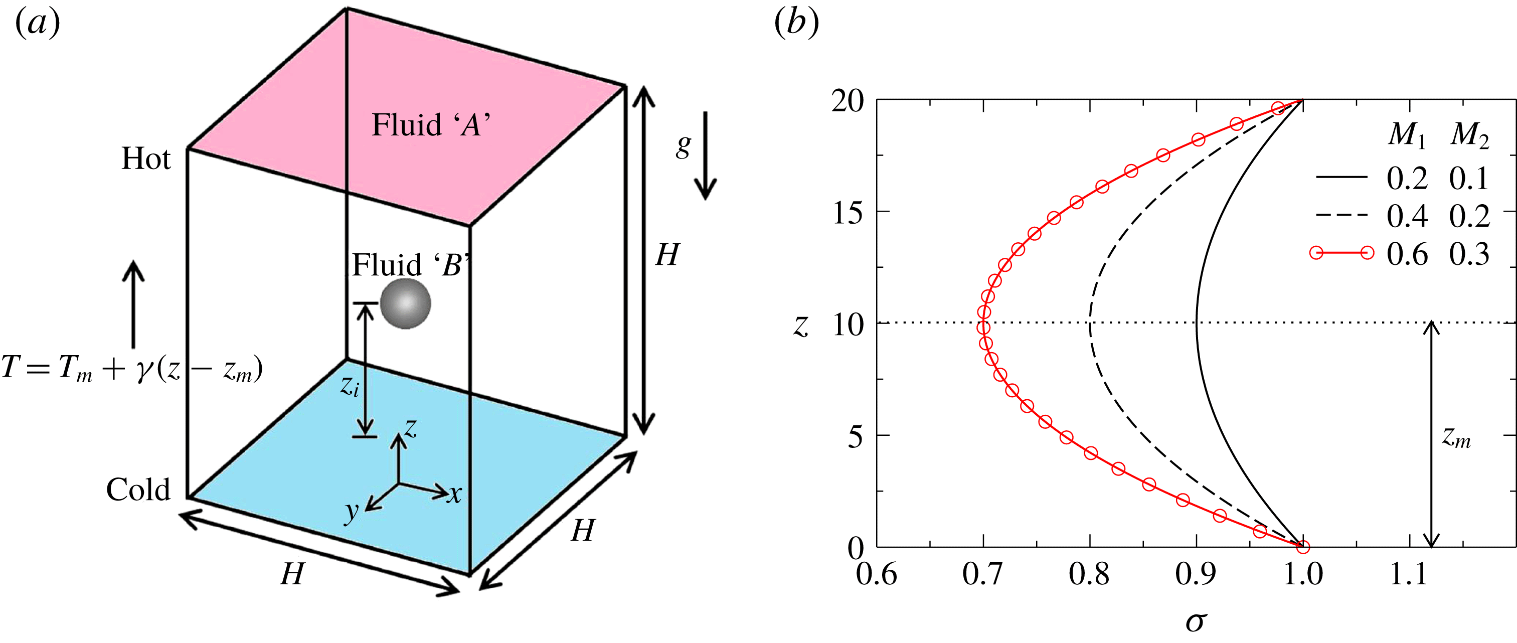
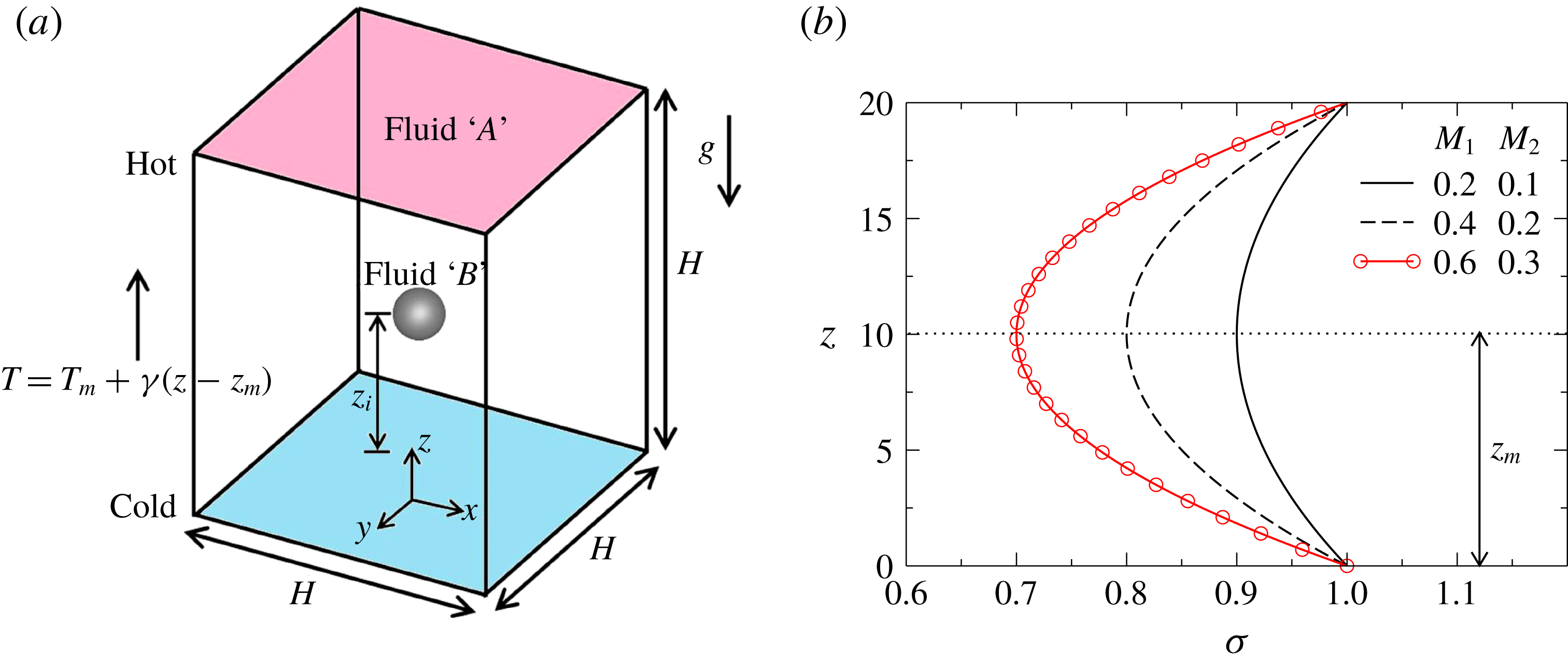
We investigate the motion of a gas bubble (fluid
 $B$
) of initial radius
 $R$
inside a cubic channel (with
 $H=20R$
, as shown in figure 1
a) filled with an incompressible, Newtonian liquid
 $A$
via three-dimensional numerical simulations. The dynamics is due to the simultaneous action of buoyancy and surface tension variation resulting due to an imposed temperature gradient via the viscous force. The surrounding fluid
 $A$
is a self-rewetting fluid whose surface tension exhibits a parabolic dependence on temperature with a well-defined minimum at
 $z_{m}$
(see figure 1
b). A Cartesian coordinate system
 $(x,y,z)$
is used to describe the bubble dynamics. Initially, the bubble is located at
 $z=z_{i}$
. The rigid and impermeable walls are located at
 $x=\pm H/2$
and
 $y=\pm H/2$
. The acceleration due to gravity,
 $g$
, acts in the negative
 $z$
direction, as shown in figure 1(a). A linear temperature variation with a constant gradient,
 $\unicode[STIX]{x1D6FE}$
, is imposed at the walls in the vertical direction, given by
 $T=T_{m}+\unicode[STIX]{x1D6FE}(z-z_{m})$
, such that
 $T_{m}$
is the temperature at the location where the surface tension is minimum, i.e.
 $z=z_{m}$
.
(a) Schematic diagram showing the initial configuration of a gas bubble (fluid
 $B$
) rising inside a liquid medium (fluid
 $A$
). Initially, the bubble is placed at
 $z=z_{i}$
inside the cubic computational domain. The acceleration due to gravity,
 $g$
, acts in the negative
 $z$
direction. A linear temperature variation is imposed at the walls in the vertical direction with a constant gradient,
 $\unicode[STIX]{x1D6FE}$
. (b) Typical variations of surface tension,
 $\unicode[STIX]{x1D70E}$
, of a self-rewetting fluid along the vertical direction for different values of
 $M_{1}$
and
 $M_{2}$
.
In order to determine the flow characteristics, we solve the equations of conservation of mass, momentum and energy, which are given by
 $$\begin{eqnarray}\displaystyle & \displaystyle \unicode[STIX]{x1D735}\boldsymbol{\cdot }\boldsymbol{u}=0, & \displaystyle\end{eqnarray}$$
 $$\begin{eqnarray}\displaystyle & \displaystyle \unicode[STIX]{x1D70C}\left[\frac{\unicode[STIX]{x2202}\boldsymbol{u}}{\unicode[STIX]{x2202}t}+\boldsymbol{u}\boldsymbol{\cdot }\unicode[STIX]{x1D735}\boldsymbol{u}\right]=-\unicode[STIX]{x1D735}p+\unicode[STIX]{x1D735}\boldsymbol{\cdot }[\unicode[STIX]{x1D707}(\unicode[STIX]{x1D735}\boldsymbol{u}+\unicode[STIX]{x1D735}\boldsymbol{u}^{\text{T}})]+\boldsymbol{F}, & \displaystyle\end{eqnarray}$$
 $$\begin{eqnarray}\displaystyle & \displaystyle \frac{\unicode[STIX]{x2202}T}{\unicode[STIX]{x2202}t}+\boldsymbol{u}\boldsymbol{\cdot }\unicode[STIX]{x1D735}T=\unicode[STIX]{x1D735}\boldsymbol{\cdot }(\unicode[STIX]{x1D6FC}\unicode[STIX]{x1D735}T). & \displaystyle\end{eqnarray}$$
Here
 $\unicode[STIX]{x1D70C}$
,
 $\unicode[STIX]{x1D707}$
and
 $\unicode[STIX]{x1D6FC}$
denote the density, viscosity and thermal diffusivity, respectively;
 $\boldsymbol{u}$
,
 $p$
and
 $T$
denote the velocity, pressure and temperature fields of the fluid, respectively; and
 $t$
represents time. The continuum surface force formulation (Brackbill, Kothe & Zemach Reference Brackbill, Kothe and Zemach1992) is used to include the surface tension force in the Navier–Stokes equations. Force
 $\boldsymbol{F}$
is the combination of gravitational force per unit volume
 $(-\unicode[STIX]{x1D70C}g\boldsymbol{e}_{\boldsymbol{z}})$
and surface tension force per unit volume
 $(\unicode[STIX]{x1D6FF}(\boldsymbol{x}-\boldsymbol{x}_{f})\unicode[STIX]{x1D70E}\unicode[STIX]{x1D705}\boldsymbol{n}+\unicode[STIX]{x1D6FF}(\boldsymbol{x}-\boldsymbol{x}_{f})\unicode[STIX]{x1D735}_{\!\!s}\unicode[STIX]{x1D70E})$
. Here,
 $\unicode[STIX]{x1D6FF}(\boldsymbol{x}-\boldsymbol{x}_{f})$
is a delta distribution (denoted by
 $\unicode[STIX]{x1D6FF}$
hereafter) that is zero everywhere except at the interface, where
 $\boldsymbol{x}=\boldsymbol{x}_{f}$
is the position vector of a point at the interface;
 $\unicode[STIX]{x1D705}=\unicode[STIX]{x1D735}\boldsymbol{\cdot }\boldsymbol{n}$
is the curvature, where
 $\boldsymbol{n}$
is the unit normal to the interface pointing towards fluid
 $A$
;
 $\boldsymbol{e}_{z}$
represents the unit vector in the vertically upward direction;
 $\unicode[STIX]{x1D735}_{\!\!s}~(\equiv \unicode[STIX]{x1D735}-(\unicode[STIX]{x1D735}\boldsymbol{\cdot }\boldsymbol{n})\boldsymbol{n})$
represents the surface gradient operator; and
 $\unicode[STIX]{x1D70E}$
represents the interfacial tension coefficient of the liquid–gas interface. The following functional dependence of the surface tension on temperature is used to model the behaviour of a self-rewetting fluid:
 $$\begin{eqnarray}\unicode[STIX]{x1D70E}=\unicode[STIX]{x1D70E}_{0}-\unicode[STIX]{x1D6FD}_{1}(T-T_{1})+\unicode[STIX]{x1D6FD}_{2}(T-T_{1})^{2}.\end{eqnarray}$$
Here
 $\unicode[STIX]{x1D6FD}_{1}\equiv -\text{d}\unicode[STIX]{x1D70E}/\text{d}T\big|_{T_{1}}$
and
 $\unicode[STIX]{x1D6FD}_{2}\equiv (\text{d}^{2}\unicode[STIX]{x1D70E}/\text{d}T^{2})/2\big|_{T_{1}}$
;
 $T_{1}=T_{m}-\unicode[STIX]{x1D6FE}z_{m}$
denotes the temperature at the bottom of the physical domain (
 $z=0$
); and
 $\unicode[STIX]{x1D70E}_{0}$
denotes the surface tension at that temperature. This parabolic dependence of the surface tension on temperature is expected to alter the type of Marangoni flow observed in the case of simple linear fluids that exhibit a linear variation of
 $\unicode[STIX]{x1D70E}$
with
 $T$
.
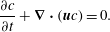
The following advection equation of the volume fraction of the liquid phase,
 $c$
, which takes on values between 0 and 1 for the gas and liquid phases, respectively, is solved using a VoF framework in order to track the interface separating the liquid and gaseous phases:
 $$\begin{eqnarray}\frac{\unicode[STIX]{x2202}c}{\unicode[STIX]{x2202}t}+\unicode[STIX]{x1D735}\boldsymbol{\cdot }(\boldsymbol{u}c)=0.\end{eqnarray}$$
As shown by Popinet (Reference Popinet2009), this equation is equivalent to the advection equation for the density. The viscosity dependence on the temperature and the volume fraction of the liquid phase is given by (Nahme Reference Nahme1940; Tripathi et al. Reference Tripathi, Sahu, Karapetsas, Sefiane and Matar2015c ):
 $$\begin{eqnarray}\unicode[STIX]{x1D707}=c\unicode[STIX]{x1D707}_{A}\text{e}^{-(T-T_{1})/(T_{m}-T_{1})}+(1-c)\unicode[STIX]{x1D707}_{B}\left\{1+\left(\frac{T-T_{1}}{T_{m}-T_{1}}\right)^{3/2}\right\},\end{eqnarray}$$
where
 $\unicode[STIX]{x1D707}_{A}$
and
 $\unicode[STIX]{x1D707}_{B}$
are the viscosity of the liquid and gaseous phases at the reference temperature,
 $T_{1}$
.
The density and thermal diffusivity are assumed to be constants for each phase, and are given by
 $$\begin{eqnarray}\displaystyle & \displaystyle \unicode[STIX]{x1D70C}=\unicode[STIX]{x1D70C}_{A}c+\unicode[STIX]{x1D70C}_{B}(1-c), & \displaystyle\end{eqnarray}$$
 $$\begin{eqnarray}\displaystyle & \displaystyle \unicode[STIX]{x1D6FC}=\unicode[STIX]{x1D6FC}_{A}c+\unicode[STIX]{x1D6FC}_{B}(1-c), & \displaystyle\end{eqnarray}$$
respectively. Here,
 $\unicode[STIX]{x1D70C}_{A}$
and
 $\unicode[STIX]{x1D70C}_{B}$
denote the density, and
 $\unicode[STIX]{x1D6FC}_{A}$
and
 $\unicode[STIX]{x1D6FC}_{B}$
represent the thermal diffusivity of the liquid and gaseous phases, respectively.
2.2 Scaling
We employ the following scaling in order to render the governing equations dimensionless:
 $$\begin{eqnarray}\left.\begin{array}{@{}c@{}}\displaystyle (x,y,z,z_{i},z_{m})=R(\widetilde{x},\widetilde{y},\widetilde{z},\widetilde{z}_{i},\widetilde{z}_{m}),\quad t=t_{s}\widetilde{t},\quad \boldsymbol{u}=V\widetilde{\boldsymbol{u}},\quad p=\unicode[STIX]{x1D70C}_{A}V^{2}\widetilde{p},\\ \displaystyle \unicode[STIX]{x1D707}=\unicode[STIX]{x1D707}_{A}\widetilde{\unicode[STIX]{x1D707}},\quad \unicode[STIX]{x1D70C}=\unicode[STIX]{x1D70C}_{A}\widetilde{\unicode[STIX]{x1D70C}},\quad \unicode[STIX]{x1D6FC}=\unicode[STIX]{x1D6FC}_{A}\widetilde{\unicode[STIX]{x1D6FC}},\quad T=\widetilde{T}(T_{m}-T_{1})+T_{1},\\ \displaystyle \unicode[STIX]{x1D70E}=\unicode[STIX]{x1D70E}_{0}\widetilde{\unicode[STIX]{x1D70E}},\quad \unicode[STIX]{x1D6FD}_{1}=\frac{\unicode[STIX]{x1D70E}_{0}}{T_{m}-T_{1}}M_{1},\quad \unicode[STIX]{x1D6FD}_{2}=\frac{\unicode[STIX]{x1D70E}_{0}}{(T_{m}-T_{1})^{2}}M_{2},\quad \unicode[STIX]{x1D6FE}=\frac{\unicode[STIX]{x1D6E4}(T_{m}-T_{1})}{R},\end{array}\right\}\end{eqnarray}$$
where tildes designate dimensionless quantities. The velocity scale,
 $V$
, is
 $\unicode[STIX]{x1D6FD}_{1}\unicode[STIX]{x1D6FE}R/\unicode[STIX]{x1D707}_{A}$
and the time scale,
 $t_{s}$
, is
 $\unicode[STIX]{x1D707}_{A}/\unicode[STIX]{x1D6FD}_{1}\unicode[STIX]{x1D6FE}$
. Here,
 $M_{1}$
,
 $M_{2}$
and
 $\unicode[STIX]{x1D6E4}$
represent the dimensionless
 $\unicode[STIX]{x1D6FD}_{1}$
,
 $\unicode[STIX]{x1D6FD}_{2}$
and imposed temperature gradient at the sidewalls in the
 $z$
direction (
 $\unicode[STIX]{x1D6FE}$
), respectively. We now drop the tilde notation from all the dimensionless quantities given in (2.9). Therefore, the variables presented hereafter in the paper are all dimensionless.
The governing dimensionless equations are given by
 $$\begin{eqnarray}\displaystyle & \displaystyle \unicode[STIX]{x1D735}\boldsymbol{\cdot }\boldsymbol{u}=0, & \displaystyle\end{eqnarray}$$
 $$\begin{eqnarray}\displaystyle & \displaystyle \unicode[STIX]{x1D70C}\left[\frac{\unicode[STIX]{x2202}\boldsymbol{u}}{\unicode[STIX]{x2202}t}+\boldsymbol{u}\boldsymbol{\cdot }\unicode[STIX]{x1D735}\boldsymbol{u}\right]=-\unicode[STIX]{x1D735}p+\frac{1}{Re}\unicode[STIX]{x1D735}\boldsymbol{\cdot }[\unicode[STIX]{x1D707}(\unicode[STIX]{x1D735}\boldsymbol{u}+\unicode[STIX]{x1D735}\boldsymbol{u}^{\text{T}})]+\frac{1}{Fr}\boldsymbol{F}, & \displaystyle\end{eqnarray}$$
 $$\begin{eqnarray}\displaystyle & \displaystyle \frac{\unicode[STIX]{x2202}T}{\unicode[STIX]{x2202}t}+\boldsymbol{u}\boldsymbol{\cdot }\unicode[STIX]{x1D735}T=\frac{1}{Ma}\unicode[STIX]{x1D735}\boldsymbol{\cdot }(\unicode[STIX]{x1D6FC}\unicode[STIX]{x1D735}T), & \displaystyle\end{eqnarray}$$
where
 $Re\equiv \unicode[STIX]{x1D70C}_{A}VR/\unicode[STIX]{x1D707}_{A}$
denotes the Reynolds number,
 $Fr\equiv V^{2}/gR$
is the Froude number,
 $Ma\equiv VR/\unicode[STIX]{x1D6FC}_{A}~(\equiv RePr)$
is the Marangoni number and
 $Pr~(\equiv \unicode[STIX]{x1D707}_{A}/\unicode[STIX]{x1D70C}_{A}\unicode[STIX]{x1D6FC}_{A})$
is the Prandtl number.
The dimensionless force
 $\boldsymbol{F}$
in (2.11) is given by
 $$\begin{eqnarray}\boldsymbol{F}=\frac{\unicode[STIX]{x1D6FF}}{Bo}[\unicode[STIX]{x1D70E}\unicode[STIX]{x1D705}\boldsymbol{n}+\unicode[STIX]{x1D735}_{\!\!s}\unicode[STIX]{x1D70E}]-\unicode[STIX]{x1D70C}\boldsymbol{e}_{\boldsymbol{z}},\end{eqnarray}$$
where
 $\unicode[STIX]{x1D70E}=1-M_{1}T+M_{2}T^{2}$
and
 $Bo=\unicode[STIX]{x1D70C}_{A}gR^{2}/\unicode[STIX]{x1D70E}_{0}~(\equiv ReCa/Fr)$
;
 $Ca\equiv V\unicode[STIX]{x1D707}_{A}/\unicode[STIX]{x1D70E}_{0}$
denotes the capillary number. The first and second terms on the right-hand side of (2.13) correspond to the capillary and gravitational contributions, respectively.
The dimensionless viscosity,
 $\unicode[STIX]{x1D707}$
, is given by
 $$\begin{eqnarray}\unicode[STIX]{x1D707}=c\text{e}^{-T}+(1-c)\unicode[STIX]{x1D707}_{r}(1+T^{3/2}),\end{eqnarray}$$
where
 $\unicode[STIX]{x1D707}_{r}\equiv \unicode[STIX]{x1D707}_{B}/\unicode[STIX]{x1D707}_{A}$
is the viscosity ratio. The dimensionless density (
 $\unicode[STIX]{x1D70C}$
) and thermal diffusivity (
 $\unicode[STIX]{x1D6FC}$
) are given by (Haj-Hariri et al.
Reference Haj-Hariri, Shi and Borhan1997):
 $$\begin{eqnarray}\displaystyle & \displaystyle \unicode[STIX]{x1D70C}=c+\unicode[STIX]{x1D70C}_{r}(1-c), & \displaystyle\end{eqnarray}$$
 $$\begin{eqnarray}\displaystyle & \displaystyle \unicode[STIX]{x1D6FC}=c+\unicode[STIX]{x1D6FC}_{r}(1-c), & \displaystyle\end{eqnarray}$$
respectively, where
 $\unicode[STIX]{x1D70C}_{r}\equiv \unicode[STIX]{x1D70C}_{B}/\unicode[STIX]{x1D70C}_{A}$
and
 $\unicode[STIX]{x1D6FC}_{r}\equiv \unicode[STIX]{x1D6FC}_{B}/\unicode[STIX]{x1D6FC}_{A}$
.
3 Numerical method
For the purposes of the present work, we have used, as a starting point, an open-source finite-volume VoF-based multiphase flow solver, Basilisk (Popinet Reference Popinet2003, Reference Popinet2009). As already pointed out, identifying the exact values of the surface tension coefficient and evaluating its gradient along the interface are quite challenging for interface capturing techniques and were not included in the original Basilisk solver. Following a similar methodology to Tripathi & Sahu (Reference Tripathi and Sahu2018), we have fully taken into account the tangential gradient of surface tension force (Marangoni force) in our calculations. The reader is referred to Tripathi & Sahu (Reference Tripathi and Sahu2018) for a detailed description of the numerical method used in the present study.
The VoF advection algorithm employed is non-diffusive and conservative in nature (Weymouth & Yue Reference Weymouth and Yue2010). The calculation of surface tension force is balanced by pressure gradient with a height-function-based interface curvature estimation. An adaptive refinement of the mesh near the interface and regions with vortical flow is used in the present study.
The following boundary conditions (in dimensionless form) are used in our numerical simulations. No-slip and no-penetration boundary conditions are imposed at all the sidewalls, and Neumann boundary conditions for temperature and for the velocity components are used at the top and bottom of the computational domain. A constant temperature
 $(T=1+\unicode[STIX]{x1D6E4}(z-z_{m}))$
is imposed at all the sidewalls. However, the boundary conditions used in § 3.1 only are different. They are prescribed in the same way as considered by the previous studies, which are explicitly discussed below.
3.1 Validations
In order to validate the present solver, first we compare the terminal velocity of a bubble migrating in a linear fluid
 $(M_{2}=0)$
due to an imposed temperature gradient in the creeping flow regime and zero Marangoni number with the corresponding theoretical prediction of Young et al. (Reference Young, Goldstein and Block1959). This test case is performed in the zero-gravity condition, as Young et al. (Reference Young, Goldstein and Block1959) theoretically derived the terminal velocity of a neutrally buoyant spherical bubble inside another infinitely unbounded fluid at rest.
The dimensionless theoretical terminal velocity of the bubble is (Young et al. Reference Young, Goldstein and Block1959)
 $$\begin{eqnarray}w_{YGB}=\frac{2}{(2+\unicode[STIX]{x1D6FC}_{r})+(2+3\unicode[STIX]{x1D707}_{r}/\unicode[STIX]{x1D70C}_{r})}.\end{eqnarray}$$
Herrmann et al. (Reference Herrmann, Lopez, Brady and Raessi2008b
) also performed numerical simulations to validate their result against the theoretical prediction of Young et al. (Reference Young, Goldstein and Block1959). Based on the configuration used by Herrmann et al. (Reference Herrmann, Lopez, Brady and Raessi2008b
), in our simulation a time-invariant linear temperature field (
 $T=1+\unicode[STIX]{x1D6E4}(z-15)$
) is imposed, which drives a bubble from the low-temperature to the high-temperature region, and the case of a linear fluid is also considered. Initially, the bubble is kept at the centre of a computational domain of size
 $15\times 15\times 15$
. The values of the dimensionless parameters are
 $\unicode[STIX]{x1D6E4}=Ca=Re=1/15$
. The rest of the parameters considered in the numerical simulation are
 $\unicode[STIX]{x1D6FC}_{r}=1$
,
 $\unicode[STIX]{x1D70C}_{r}=1$
and
 $\unicode[STIX]{x1D707}_{r}=1$
. For this set of parameters,
 $w_{YGB}\approx 0.133$
. In our three-dimensional numerical simulation, we found that the terminal velocity of the bubble
 $(w_{rise})$
is
 $0.131$
. Thus, the percentage error,
 $(1-w_{rise}/w_{YGB})\times 100$
, is less than 1.7 %.
Drop migration velocity for
 $Re=Ma=0.72$
and
 $Ca=0.0576$
in the absence of gravitational effects.
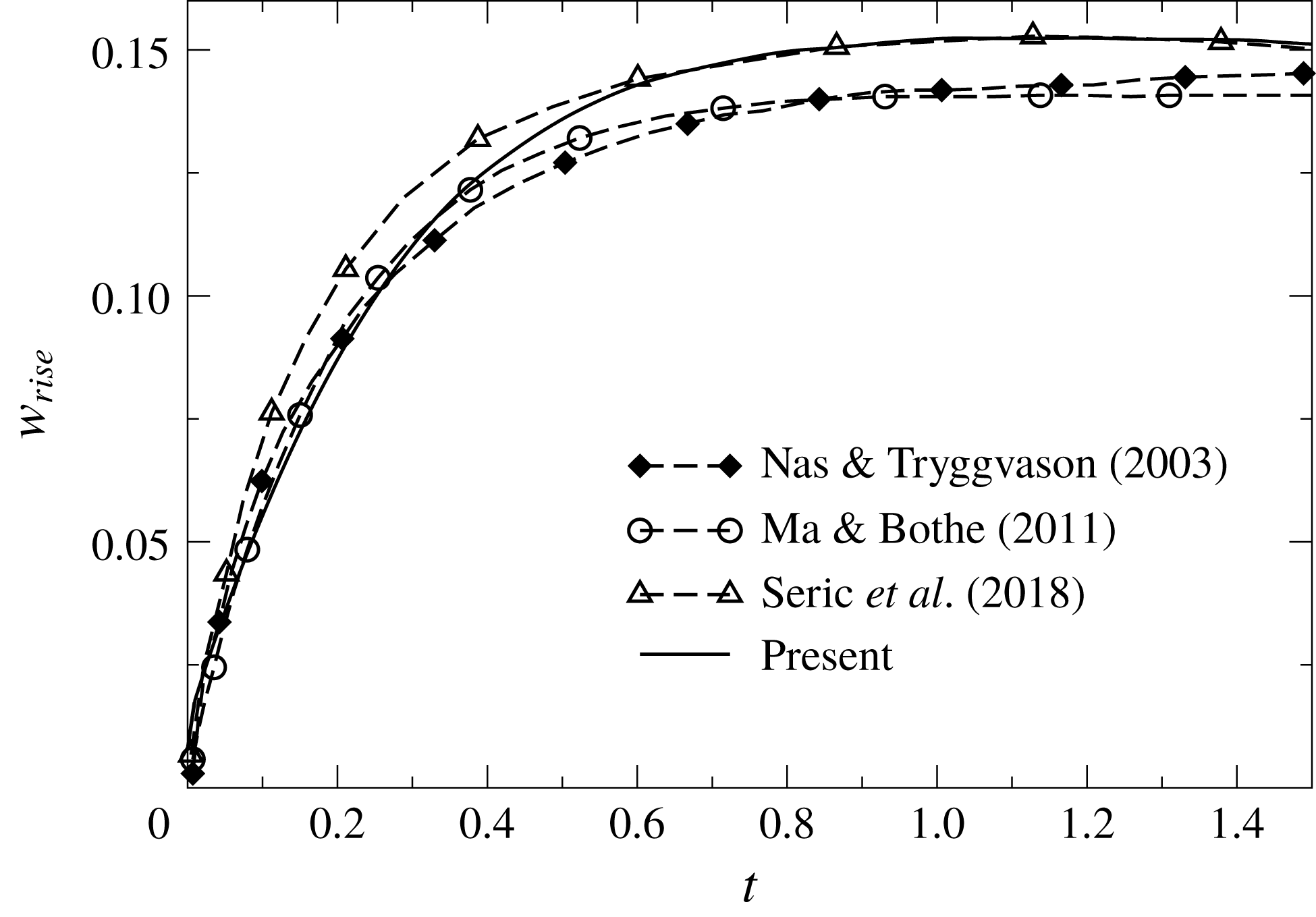
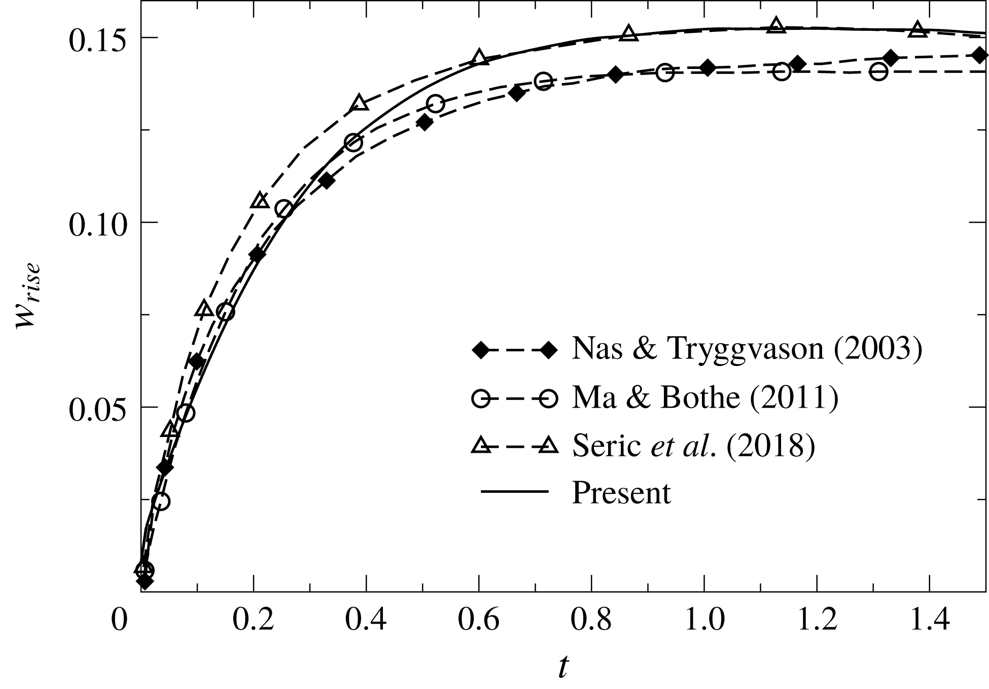
Next, we compare the rise velocity of a neutrally buoyant spherical bubble obtained from our numerical simulation with that reported by the previous studies in figure 2. The parameter values considered for this test case are
 $Re=Ma=0.72$
and
 $Ca=0.0576$
. The ratio of the fluid properties of the ambient fluid with those of the drop is fixed at 2. This test case was originally taken by Nas & Tryggvason (Reference Nas and Tryggvason2003) and subsequently used by other researchers (see e.g. Ma & Bothe Reference Ma and Bothe2011; Seric et al.
Reference Seric, Afkhami and Kondic2018) to validate their numerical solvers. A square computational domain of size
 $4\times 4$
is considered. As considered by the previous studies, two-dimensional simulation is performed for this exercise. No-slip and no-penetration boundary conditions are used at the top and bottom walls, whereas Neumann boundary conditions for the velocity components and temperature are used at the side boundaries. A grid convergence test is performed and the converged solution is obtained using a grid size (dimensionless)
 $\unicode[STIX]{x1D6E5}=0.0312$
. It can be seen in figure 2 that the terminal rise velocity obtained from our simulation agrees well that of Seric et al. (Reference Seric, Afkhami and Kondic2018). However, in the accelerating regime (
 $t<0.4$
), our result is closer to those of Nas & Tryggvason (Reference Nas and Tryggvason2003) and Ma & Bothe (Reference Ma and Bothe2011).
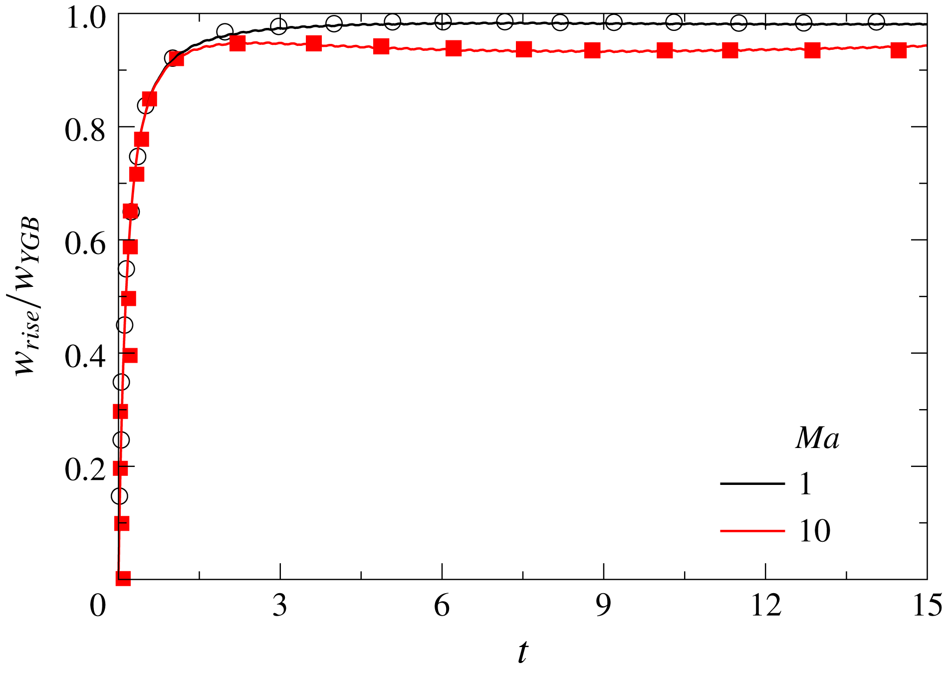
The temporal variations of the normalised velocity of the bubble,
 $w_{rise}/w_{YGB}$
, for
 $Ma=1$
and 10. The rest of the parameters are
 $Re=1$
,
 $Ca=0.1$
and
 $\unicode[STIX]{x1D6E4}\approx 0.133$
. The symbols are the results of Liu et al. (Reference Liu, Zhang and Valocchi2012) and the solid lines represent our results.
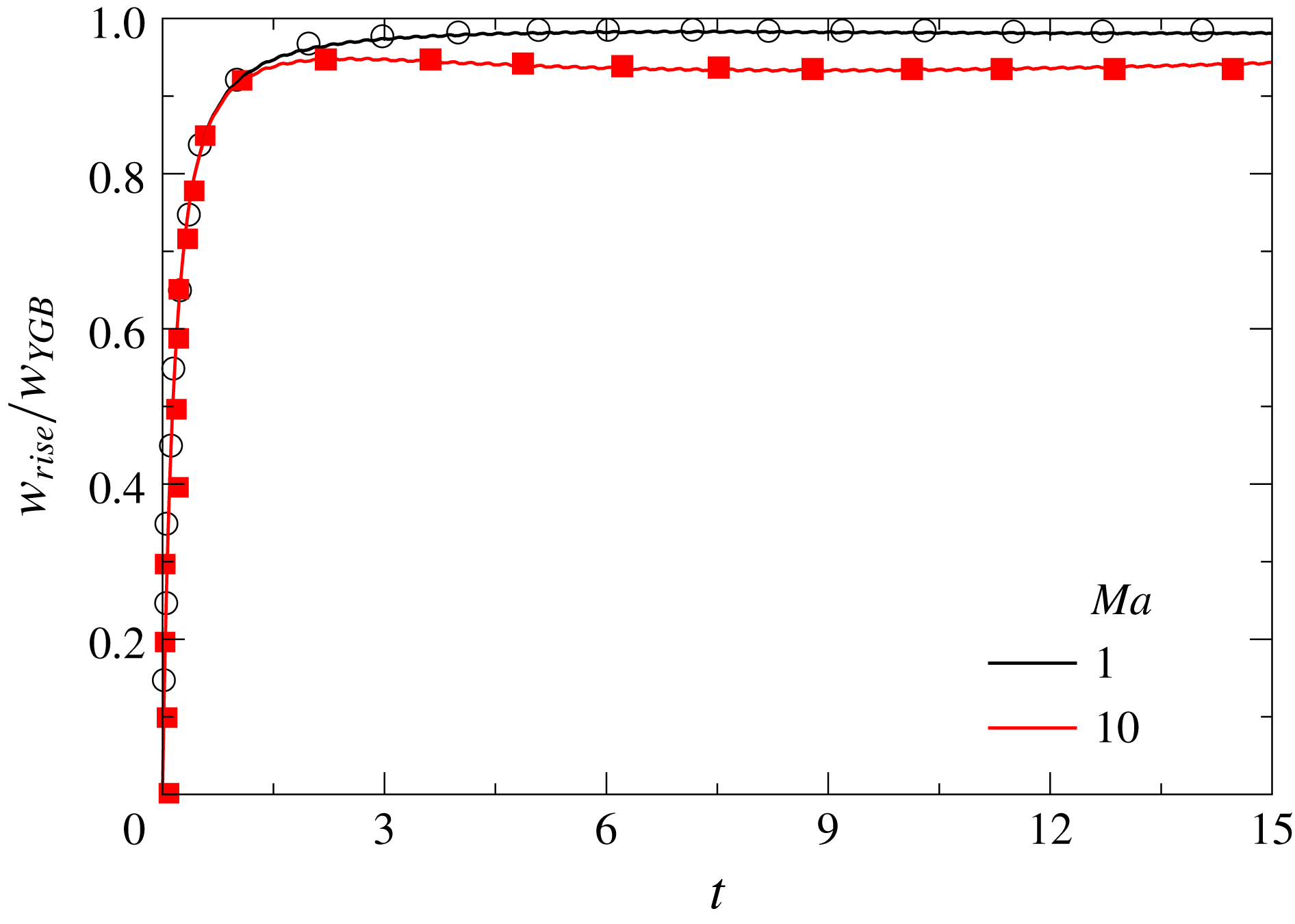
We have also performed a validation exercise by comparing the thermocapillary migration of a bubble obtained from the present simulation with that of Liu et al. (Reference Liu, Zhang and Valocchi2012). They conducted simulations based on the lattice Boltzmann method for the thermocapillary migration of a bubble placed at the centre of a computational domain of size
 $15R\times 15R\times 15R$
with the top and bottom walls maintained at temperatures 0 and 24 (lattice units), respectively. They used
 $R=16$
,
 $\unicode[STIX]{x1D70C}_{A}=\unicode[STIX]{x1D70C}_{B}=1.0$
,
 $\unicode[STIX]{x1D707}_{A}=\unicode[STIX]{x1D707}_{B}=0.2$
,
 $\unicode[STIX]{x1D70E}_{0}=0.025$
and
 $T_{ref}=12$
; all the variables are in lattice units. This gives
 $Re=1$
,
 $Ca=0.1$
and
 $\unicode[STIX]{x1D6E4}=0.13333$
. The thermal conductivity of the fluids,
 $\unicode[STIX]{x1D705}_{A}=\unicode[STIX]{x1D705}_{B}=0.2$
and 0.02, are used to obtain
 $Ma=1$
and 10. We performed numerical simulations for these sets of dimensionless numbers using
 $\unicode[STIX]{x1D6E5}=0.06$
(as also used in their study). No-slip and no-penetration boundary conditions are used at the top and bottom walls, and periodic boundary conditions for the velocity components and temperature are used at the side boundaries. The bubble rise velocity normalised with the theoretical result of Young et al. (Reference Young, Goldstein and Block1959) versus time for
 $Ma=1$
and 10 is plotted in figure 3. For these parameters,
 $w_{YGB}=1.667\times 10^{-4}$
. It can be seen that the agreement is quite good.
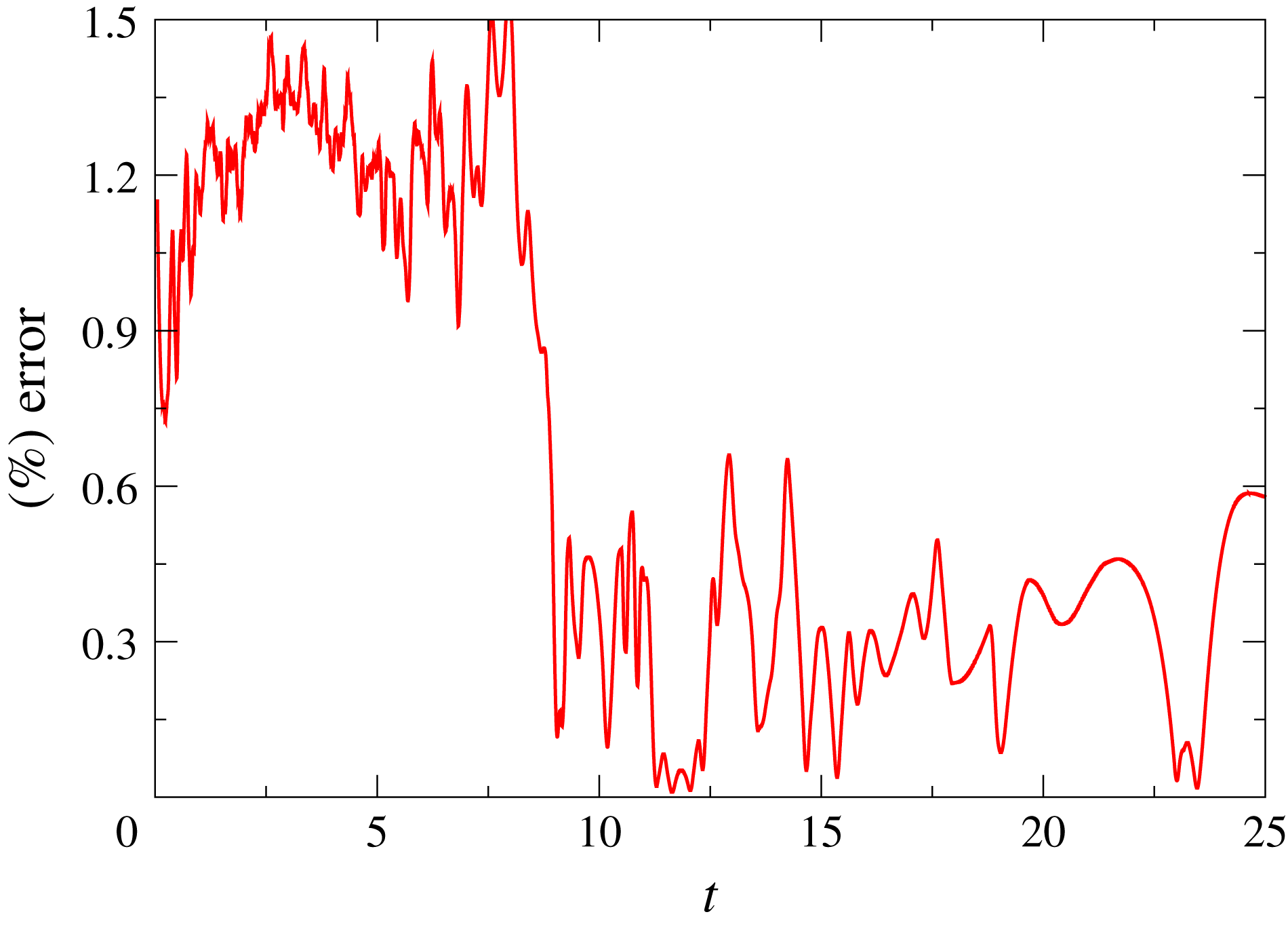
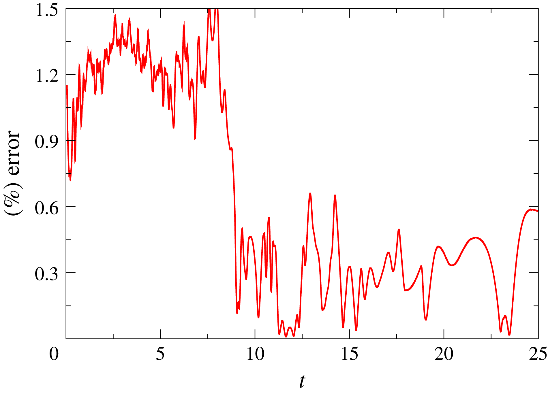
The temporal variation of the difference (in percentage) between the pressure force plus force due to normal viscous stress difference and surface tension force integrated over the entire bubble surface. Here
 $M_{1}=0.4$
and
 $M_{2}=0.2$
, and the rest of the parameters are
 $Re=10$
,
 $Bo=10^{-3}$
,
 $Fr=50$
,
 $Pr=0.7$
,
 $\unicode[STIX]{x1D707}_{r}=10^{-2}$
,
 $\unicode[STIX]{x1D70C}_{r}=10^{-3}$
,
 $\unicode[STIX]{x1D6FC}_{r}=0.04$
,
 $z_{i}=9.5$
and
 $\unicode[STIX]{x1D6E4}=0.1$
(base parameters).
To generate the results presented in the following section, a three-dimensional computation domain of size
 $20\times 20\times 20$
is used. Initially the gas bubble is placed at
 $z_{i}=z_{CG}(t=0)=9.5$
. A wavelet-error-based dynamic adaptive grid refinement feature of Basilisk has been employed to refine the grid at the interface and in the regions of the domain where the gradients in velocity are large. The refinement level used in our simulations is 6, which corresponds to 64 computational cells per unit domain width, and the finest level being 9 near the interface, which amounts to 512 computational cells per unit domain width. An intermediate refinement of 256 cells per unit domain width is used in regions with higher velocity gradients. As mentioned in Popinet (Reference Popinet2018), the balanced force method for the calculation of the surface tension term in the Navier–Stokes equations may generate parasitic currents for surface-tension-dominant flows. Thus, in figure 4, we have performed another test to check whether the capillary pressure balances the pressure jump across the interface for
 $Re=10$
,
 $Bo=10^{-3}$
,
 $Fr=50$
,
 $Pr=0.7$
,
 $\unicode[STIX]{x1D707}_{r}=10^{-2}$
,
 $\unicode[STIX]{x1D70C}_{r}=10^{-3}$
,
 $\unicode[STIX]{x1D6FC}_{r}=0.04$
,
 $z_{i}=9.5$
and
 $\unicode[STIX]{x1D6E4}=0.1$
(hereafter, termed the ‘base’ parameters). Here, the temporal variation of the percentage difference between the integral pressure jump across the interface and integral value of the capillary pressure over the bubble surface is plotted for
 $M_{1}=0.4$
and
 $M_{2}=0.2$
. This is defined as [(pressure force
 $+$
force due to normal viscous stress difference
 $-$
surface tension force)/(surface tension force)]
 $\times$
100. Note that the surface tension force includes its normal and Marangoni contributions. It can be seen that it is approximately 1.5 %, which reduces to approximately 0.5 % at later times.
4 Results and discussion
4.1 Axisymmetric bubble
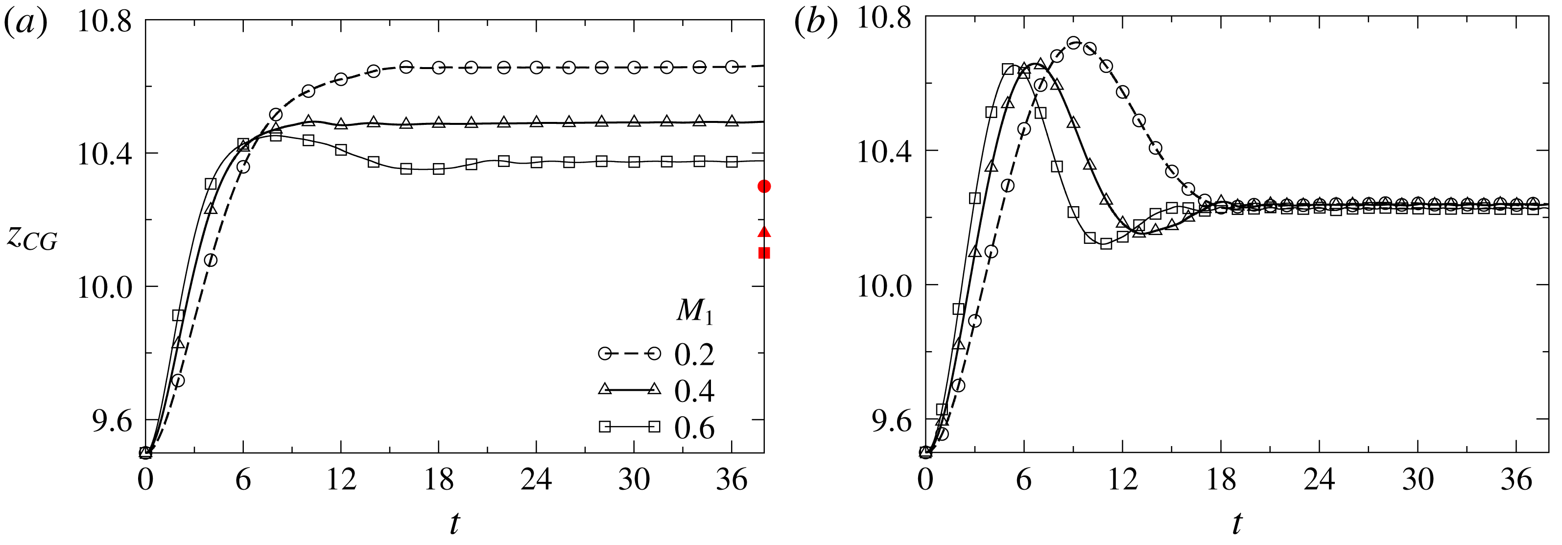
We begin the discussion of our results by examining the case of an axisymmetric gas bubble. Tripathi et al. (Reference Tripathi, Sahu, Karapetsas, Sefiane and Matar2015c ) have shown that, as the bubble crosses the position of minimum surface tension, the bubble motion could be reversed, for sufficiently small Bond number and significant inertia, and eventually becomes arrested near the position of minimum surface tension. It is important to note, though, that in their numerical simulations the contribution of the surface tension gradient term in the interfacial stress balance was neglected, and therefore one of the goals of the present study is to investigate the impact of this missing term on the nonlinear dynamics of the bubble motion. As mentioned above, our numerical scheme is able to fully account for the contributions of the Marangoni force.
Temporal variation of the centre of gravity of the bubble,
 $z_{CG}$
, rising in an axisymmetric domain. (a) With Marangoni term (
 $\unicode[STIX]{x1D6FF}\unicode[STIX]{x1D735}_{\!\!s}\unicode[STIX]{x1D70E}$
), and (b) without Marangoni term (
 $\unicode[STIX]{x1D6FF}\unicode[STIX]{x1D735}_{\!\!s}\unicode[STIX]{x1D70E}$
). The parameter values are
 $Re=10$
,
 $Bo=10^{-3}$
,
 $Fr=50$
,
 $Pr=0.7$
,
 $\unicode[STIX]{x1D707}_{r}=10^{-2}$
,
 $\unicode[STIX]{x1D70C}_{r}=10^{-3}$
,
 $\unicode[STIX]{x1D6FC}_{r}=0.04$
,
 $z_{i}=9.5$
and
 $\unicode[STIX]{x1D6E4}=0.1$
(base parameters). The positions of bubble arrest for
 $M_{1}=0.2$
, 0.4 and 0.6 obtained from the analytical solution are shown in panel (a) by the red filled circle, triangle and square, respectively, on the right-hand axis.
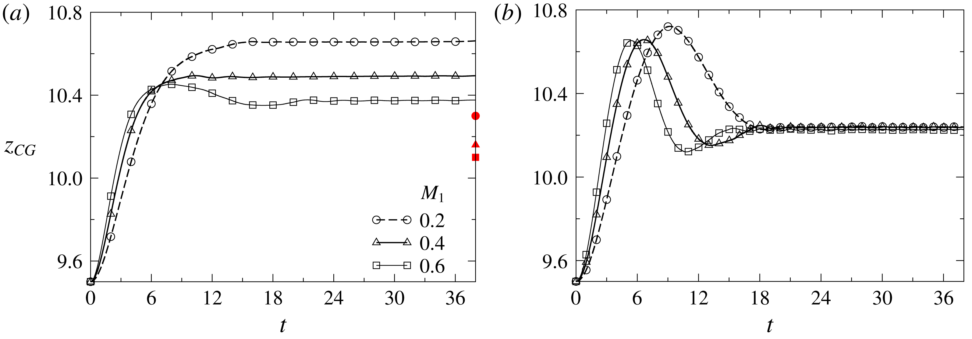
Figure 5(a,b) presents a comparison between the results obtained from the present study and those predicted by Tripathi et al. (Reference Tripathi, Sahu, Karapetsas, Sefiane and Matar2015c
), respectively. In figure 5(a,b), we depict the temporal variation of the centre of gravity,
 $z_{CG}$
, of a bubble rising in a self-rewetting fluid inside a channel with walls that are heated according to a linear temperature profile of constant gradient
 $\unicode[STIX]{x1D6E4}>0$
. The evolutions of
 $z_{CG}$
are shown for three different values of the parameter
 $M_{1}$
, while
 $M_{2}=M_{1}/2$
; the latter restriction is imposed to keep the position where the minimum surface tension occurs constant. (The remaining parameters are the same as the base parameters.) The comparison between the two sets of simulations reveals that the Marangoni stresses significantly affects the dynamics of the bubble motion. In figure 5(b), as described in Tripathi et al. (Reference Tripathi, Sahu, Karapetsas, Sefiane and Matar2015c
), the bubble reaches a maximum height (
 $z\approx 10.7$
) before it reverses its motion and equilibrates at
 $z\approx 10.24$
, for all values of
 $M_{1}$
. On the other hand, in figure 5(a), where we have included the Marangoni term in the interfacial stress balance, a significantly different behaviour is observed. For all values of
 $M_{1}$
considered, the bubble rises with a constant velocity till
 $t\approx 6$
, after a short accelerating phase initially. At later times (for
 $t>10$
, approximately), the bubble attains a terminal location and becomes stationary. It can be seen in figure 5(a) that increasing the value of
 $M_{1}$
decreases the location of bubble arrest. We also observe that the reversal of bubble motion takes place only for the highest value of
 $M_{1}$
 $(M_{1}=0.6)$
for which the effect of Marangoni stresses acting in the downward direction become maximised and overcome the effect of buoyancy before the bubble reaches its terminal position.
Tripathi et al. (Reference Tripathi, Sahu, Karapetsas, Sefiane and Matar2015c
) derived an analytical expression for the position of bubble entrapment based on the assumption of Stokes flow (see their equation (4.1)) which in our case gives
 $z=10.09$
. Besides the fact that the analytical solution takes fully into account the presence of the Marangoni contribution, the predicted value appears to be much closer to the predictions of the numerical simulation shown in figure 5(b). This seemingly puzzling situation can be explained by looking more carefully at the flow field of the liquid that surrounds the bubble in both cases. According to the Stokes limit solution, in the case of a motionless bubble there is no flow of the surrounding liquid (see equation (3.13) in Tripathi et al. (Reference Tripathi, Sahu, Karapetsas, Sefiane and Matar2015c
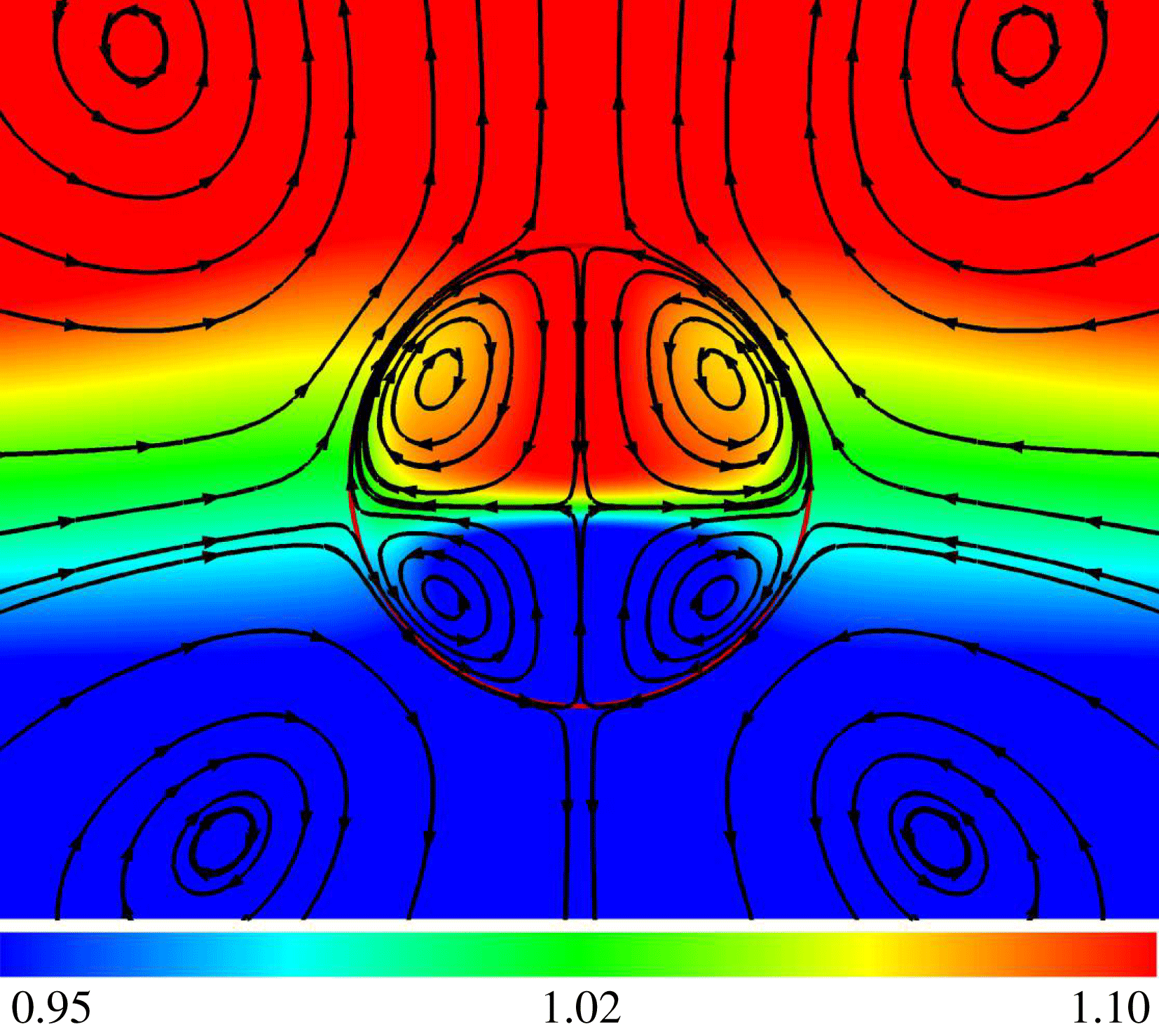
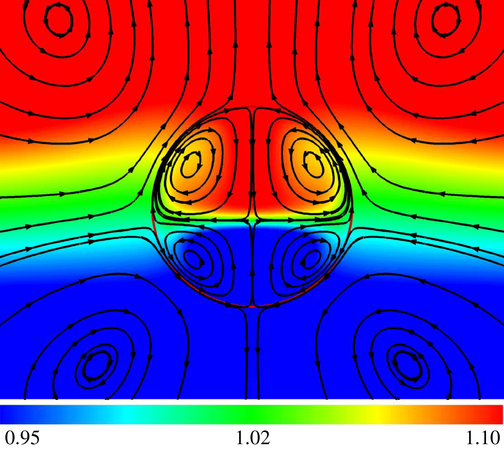
)). In the numerical simulations of figure 5(b), when the bubble reaches a motionless state, we find (not shown) that the velocity field is indeed very close to zero, which explains the good agreement with the Stokes limit solution. However, when the Marangoni term is taken into account and for finite values of
 $Re$
, the liquid is never entirely motionless since thermocapillarity drives a steady recirculation around the bubble. This is shown very clearly in figure 6 where we depict the streamlines associated with the bubble for
 $M_{1}=0.6$
at
 $t=20$
; similar streamline patterns are observed for other values of
 $M_{1}$
as well. The presence of liquid motion, even at times that the bubble has reached its equilibrium position, clearly renders the analytical solution invalid.
Streamlines at
 $t=20$
for
 $M_{1}=0.6$
fully accounting for the Marangoni term (
 $\unicode[STIX]{x1D6FF}\unicode[STIX]{x1D735}_{\!\!s}\unicode[STIX]{x1D70E}$
). The background colour shows the temperature field. The rest of the parameters are the same as those used to generate figure 5(a).
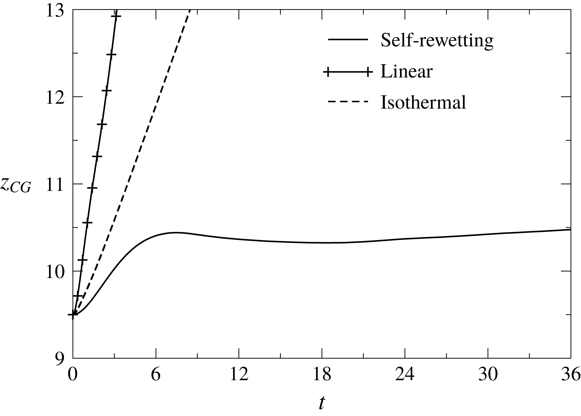
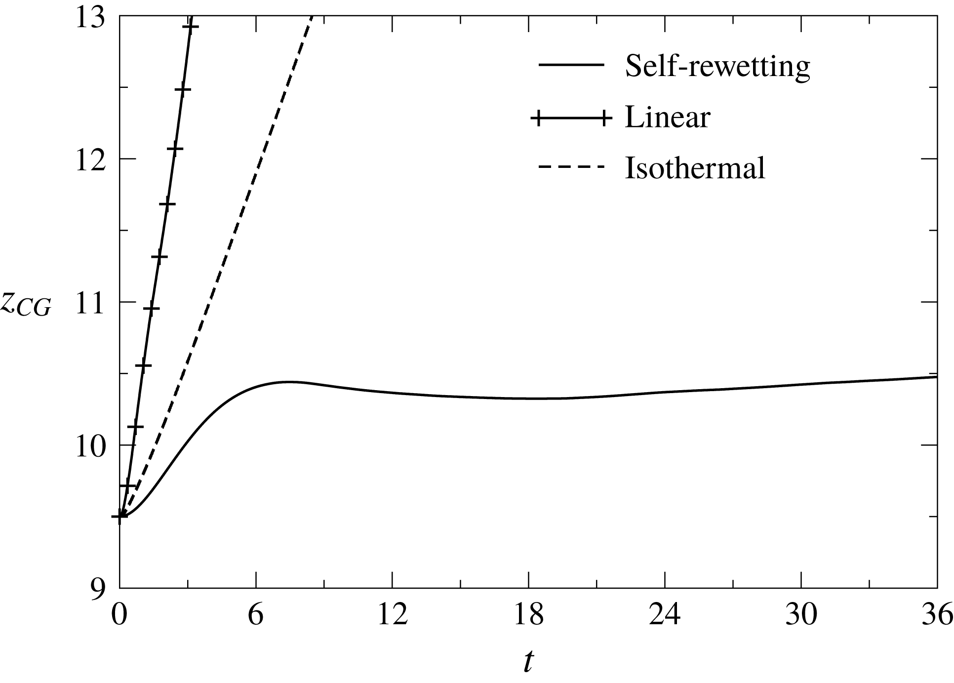
Temporal variation of the centre of gravity of the bubble for an isothermal system (
 $M_{1}=0$
and
 $M_{2}=0$
), a self-rewetting fluid (
 $M_{1}=0.4$
and
 $M_{2}=0.2$
) and a linear fluid (
 $M_{1}=0.4$
and
 $M_{2}=0$
) and
 $z_{i}=9.5$
. The remaining parameter values are the same as the base parameters.
4.2 Effects of three-dimensional flow
We now turn our attention to the three-dimensional flow, which is the main focus the present work. In figure 7, we present the temporal variation of the centre of gravity,
 $z_{CG}$
, of a rising bubble inside a rectangular channel for three different cases: the case of a bubble rising in an isothermal liquid, and the cases where the channel is filled with either a linear (
 $M_{1}=0.4$
and
 $M_{2}=0$
) or a self-rewetting fluid (
 $M_{1}=0.4$
and
 $M_{2}=0.2$
). The remaining parameters are the same as the base parameters. It can be seen that the bubble undergoes a relatively short acceleration phase, after which the bubble attains a constant terminal speed for both the isothermal and the linear fluid (non-isothermal) cases. For the linear fluid, the terminal speed is higher due to the presence of Marangoni stresses, which drive liquid towards the cold region of the channel, i.e. Marangoni stresses act in the same direction as that of buoyancy, thereby enhancing the upward motion of the bubble. For the self-rewetting fluid case, the surface tension decreases and then increases (see (2.4) and figure 1
b) with a minimum at
 $z_{m}=10$
. Thus in region
 $z>z_{m}$
, the bubble experiences a pull in the downward direction due to Marangoni stresses, but buoyancy tries to push the bubble in the upward direction. Owing to this competition between Marangoni stresses and buoyancy, the bubble moves with a considerably lower speed until, at later times
 $(t>8)$
, these forces counterbalance each other and the bubble at
 $t\approx 18$
has become entrapped at
 $z\approx 10.33$
for this set of parameters.
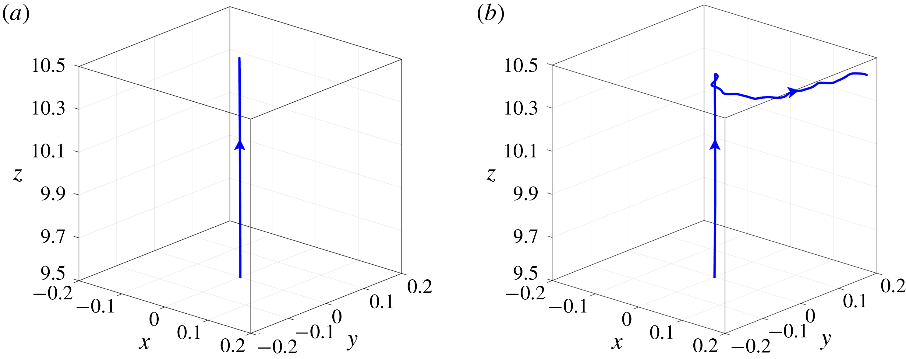
Trajectories of the bubble moving in a channel containing the (a) linear fluid (
 $M_{1}=0.4$
and
 $M_{2}=0$
) and (b) self-rewetting fluid (
 $M_{1}=0.4$
and
 $M_{2}=0.2$
). The remaining parameter values are the same as the base parameters.
It is well known that, in isothermal systems, the three-dimensionality of the flow can be expressed through a zig-zag motion of the bubble (Tripathi et al.
Reference Tripathi, Sahu and Govindarajan2015a
). However, the mechanism of the zig-zagging motion of a bubble in an isothermal system is different from that in the present case. In the case of an isothermal system, the three-dimensional motion is associated with a symmetric pair of rotating vortices in the wake of the bubble (Magnaudet & Mougin Reference Magnaudet and Mougin2007). As expected for the specific parameter values used in figure 7, the bubble in the isothermal liquid rises in a perfectly straight path (Tripathi et al.
Reference Tripathi, Sahu and Govindarajan2015a
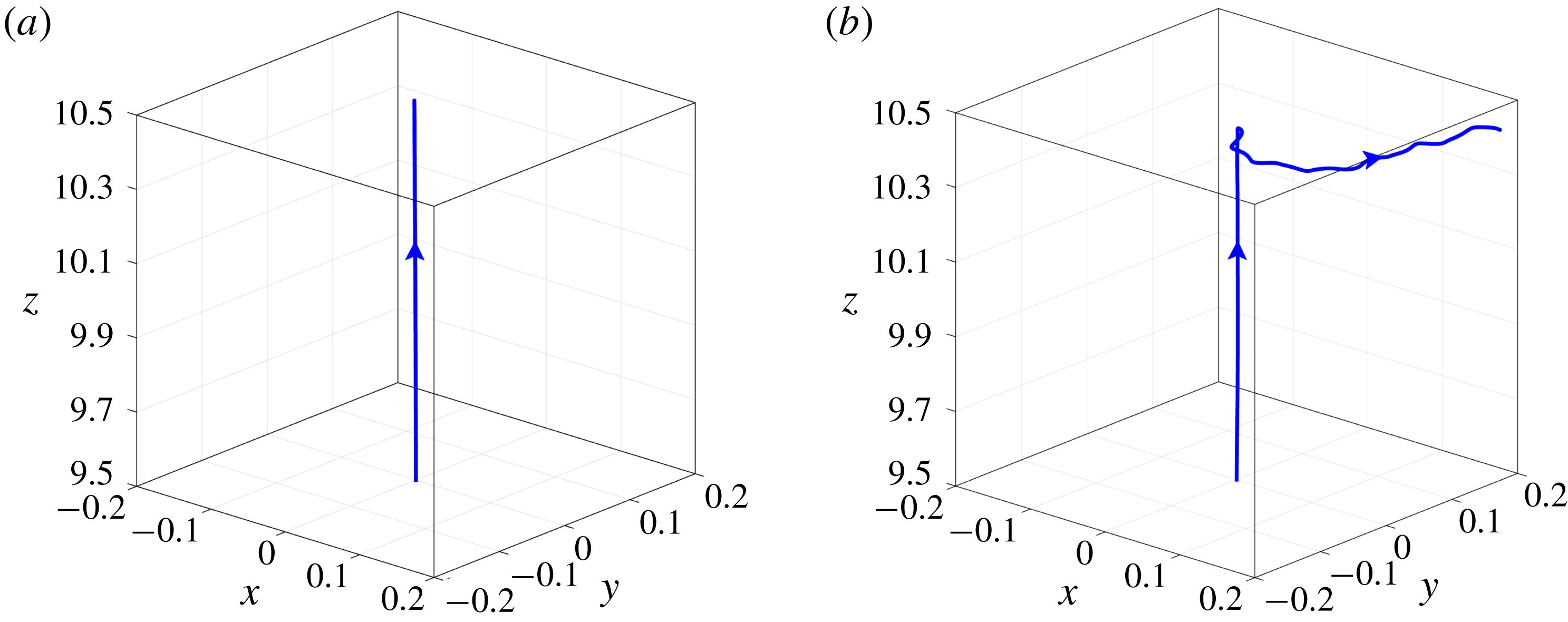
). In figure 8(a), we plot the trajectory of a bubble rising in a linear fluid (non-isothermal case). Like in the isothermal case, the bubble in a linear fluid also moves in the upward direction in an almost vertical path. On the other hand, a striking difference is observed in the case of the self-rewetting fluid (see figure 8
b), where the bubble initially moves vertically, but after its upward motion decelerates and reaches
 $z\approx 10.33$
, the bubble migrates away from the axis of symmetry. This can be explained as follows. In the returning path (after the bubble has reached its maximum height) and when the bubble reaches a stationary position, any perturbation in the position of the bubble will lead to interfacial thermal gradients. The bubble has a relatively low/high-temperature fluid in its wake due to the Marangoni convection when the bubble is rising/on the return path. This builds up a radial gradient of temperature in the vicinity of the bubble. Any perturbation in the flow may cause the bubble to experience an asymmetrical temperature distribution, which leads to an unbalanced force in the horizontal direction due to the asymmetrical Marangoni stresses. The onset of this horizontal migration may be studied in detail with the help of a linear stability analysis, which is out of the scope of the present study.
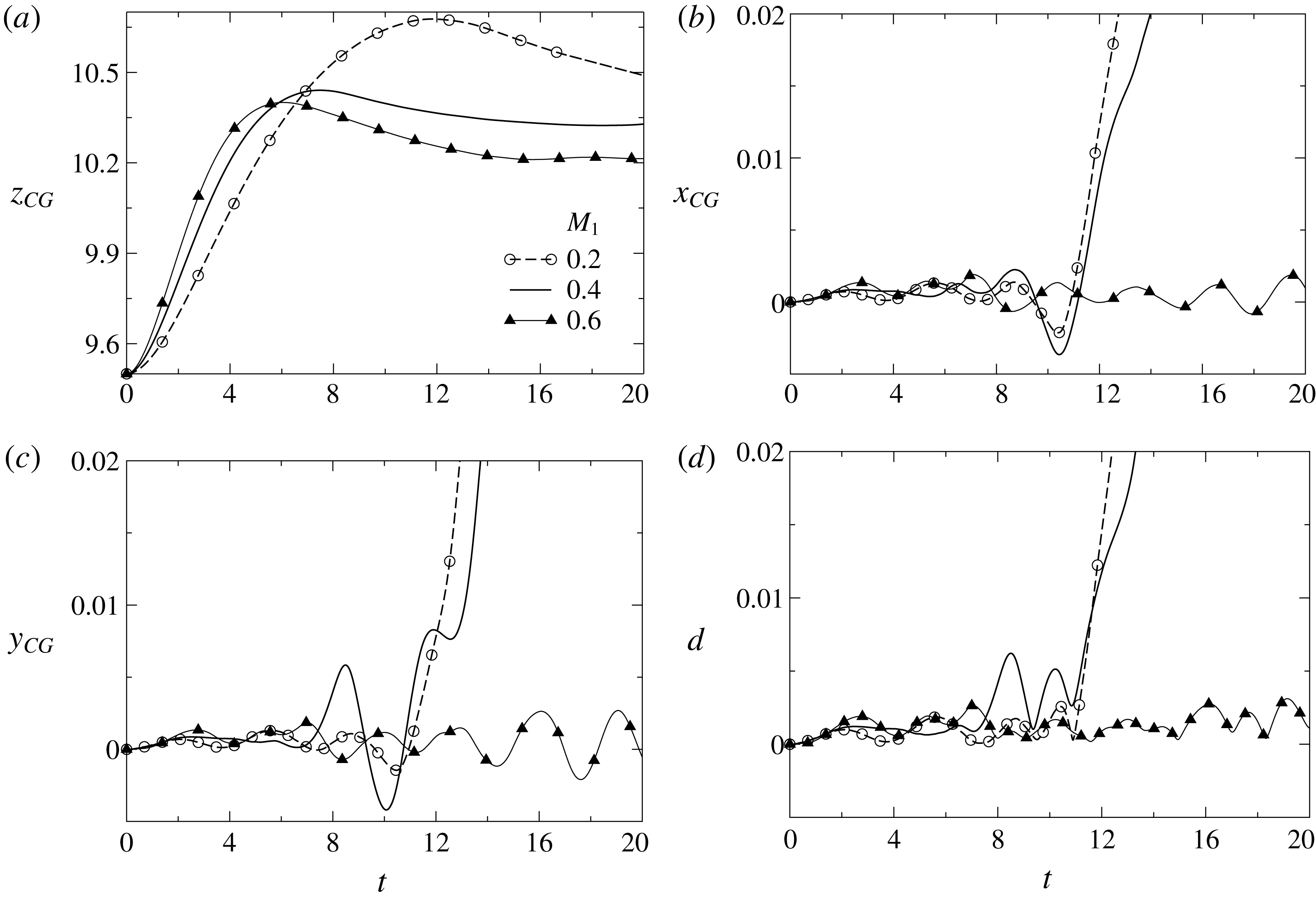
Temporal variations of (a)
 $z_{CG}$
, (b)
 $x_{CG}$
, (c)
 $y_{CG}$
and (d) the distance of the centre of gravity of the bubble from the axis,
 $d=\sqrt{x_{CG}^{2}+y_{CG}^{2}}$
, for different values of
 $M_{1}$
. The parameter values are the same as those used in figure 7 while
 $M_{2}=M_{1}/2$
.
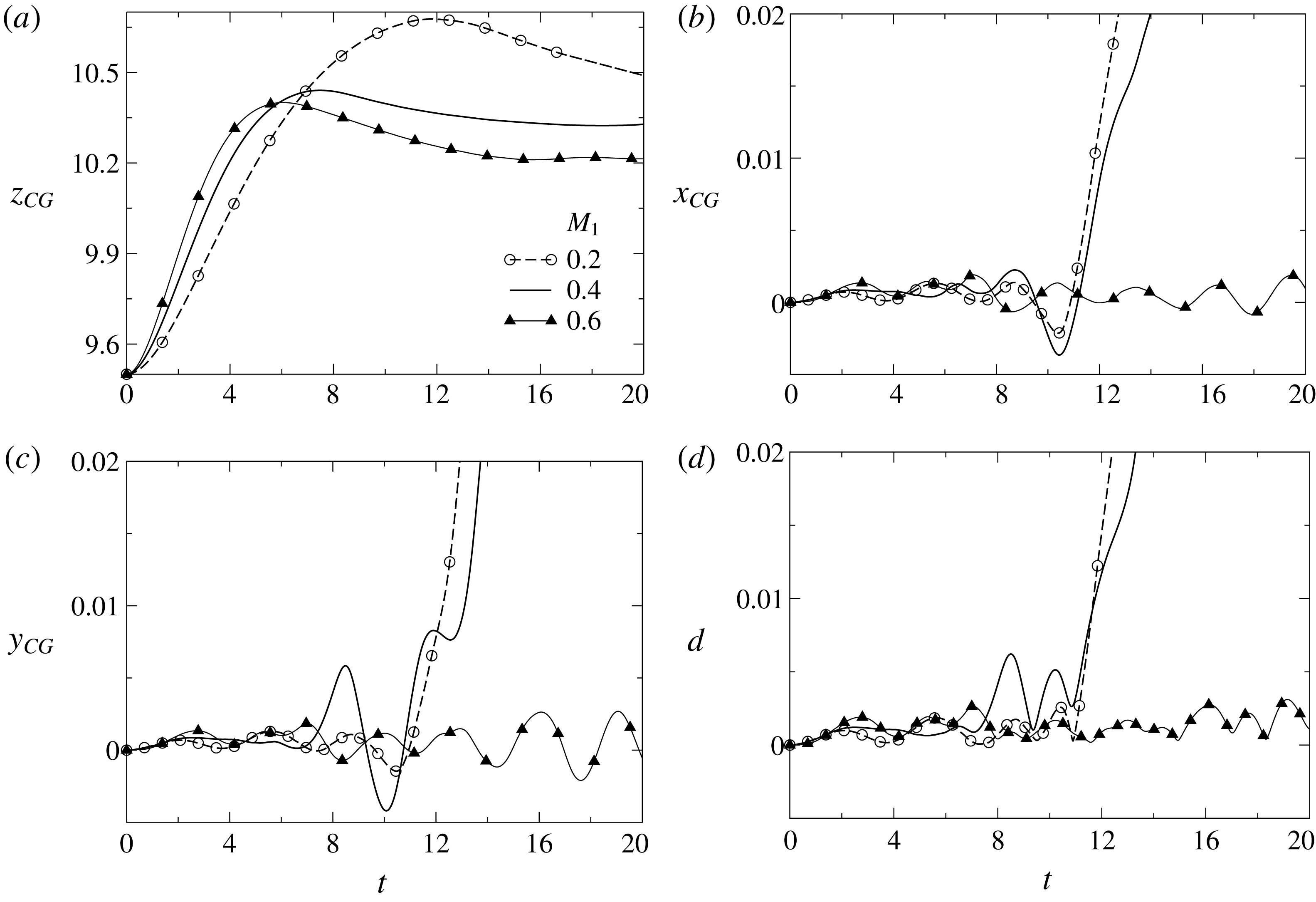
The lateral migration of the bubble is quantified in figure 9, where we plot the evolution of the
 $z$
,
 $x$
and
 $y$
components of the position of the bubble centre of gravity along with its distance from the axis,
 $d=\sqrt{x_{CG}^{2}+y_{CG}^{2}}$
, for three different values of
 $M_{1}$
and
 $M_{2}=M_{1}/2$
. It can be seen that, at early times, the bubble rises approximately vertically, i.e. along
 $(x,y)=(0,0)$
, and continues to do so even after the bubble has crossed the location where the surface tension is minimum, i.e.
 $z=z_{m}$
; in this region the thermocapillary stresses act to decelerate its upward motion (see figure 9
a). Increasing the value of
 $M_{1}$
, and thus
 $M_{2}$
as well, the rise velocity of the bubble decreases due to the fact that the self-rewetting character of the fluid becomes more pronounced and the bubble retardation due to the induced thermocapillary stresses increases. Thus, as shown in figure 9(a), the bubble is eventually arrested at lower heights. Interestingly, the first signs of bubble migration away from the axis of the channel appear when its motion in the vertical direction decelerates. In particular, for
 $M_{1}=0.2$
we find that the bubble begins its lateral motion at
 $t\approx 11$
, which coincides with the time that the bubble has reached its maximum elevation (see figures 9
a and 9
d). Similarly, for
 $M_{1}=0.4$
the bubble initiates its lateral motion at
 $t\approx 7$
, although in this case the bubble temporarily revolves around the axis of the channel, as it moves downwards. Eventually, though, as the bubble decelerates its vertical motion, it sets off moving in the lateral direction (for
 $t>12$
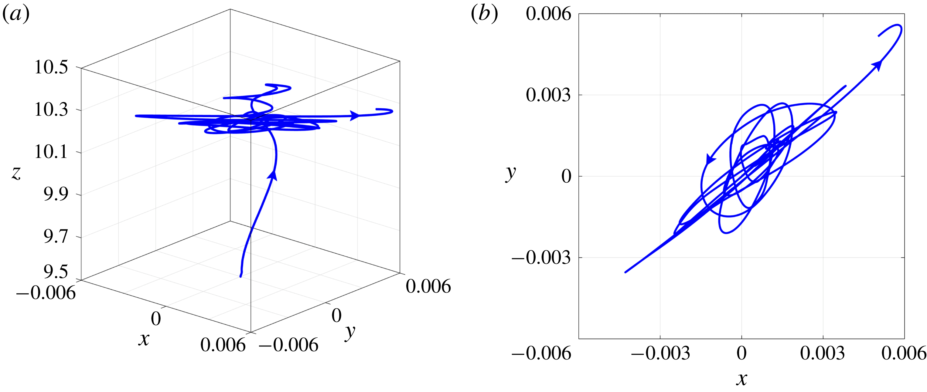
). Another strikingly different behaviour is observed in the trajectory of the bubble for
 $M_{1}=0.6$
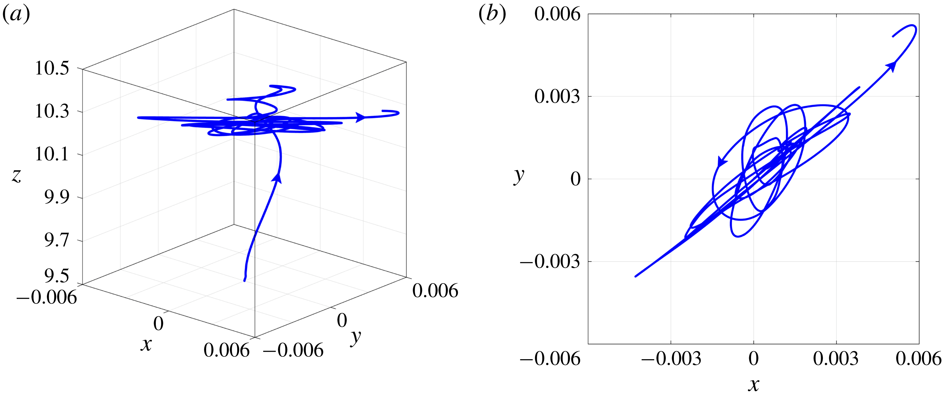
(see figure 10
a,b) from the cases with lower values of
 $M_{1}$
. For
 $M_{1}=0.6$
, the bubble undergoes spiralling motion (albeit of small amplitude), in contrast to the bubble for lower values of
 $M_{1}$
, which migrates away from the axis of symmetry in the lateral direction after rising in the vertical path in the early times (see figure 8
b).
Trajectory of the bubble. (a) Three-dimensional view, and (b) top view (projection on the
 $x$
–
 $y$
plane) for
 $M_{1}=0.6$
. The remaining parameter values are the same as the base parameters.
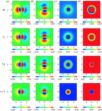
Spatio-temporal variation (bottom to top:
 $t=3$
, 7.8, 11 and 20) of
 $u$
,
 $v$
,
 $w$
and
 $T$
contours (a–d) on the
 $x$
–
 $y$
plane at
 $z_{CG}$
for the self-rewetting fluid for
 $M_{1}=0.4$
. The remaining parameter values are the same as the base parameters.
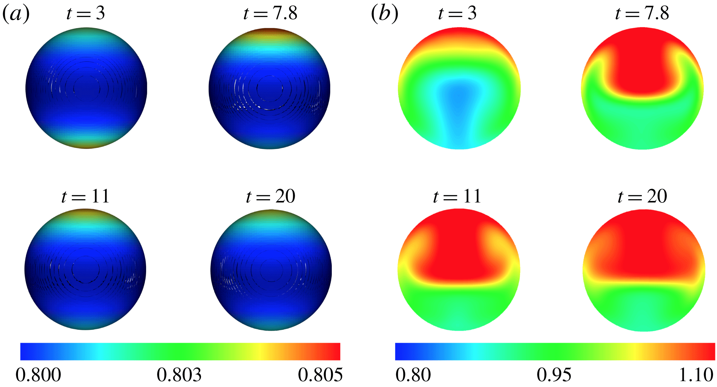
The lateral migration of buoyant drops and bubbles has also been observed in the case of isothermal systems (e.g. see Tripathi et al. (Reference Tripathi, Sahu and Govindarajan2015a ) and references therein). In these systems, it has been established that the migration and non-axisymmetric motion typically take place due to the combined effect of inertia and interfacial deformation. In our case, however, interfacial deformation cannot be held responsible since it is negligible at all times for the parameter values that are examined in the present work (for instance, see the bubble shapes at different times in figure 11).
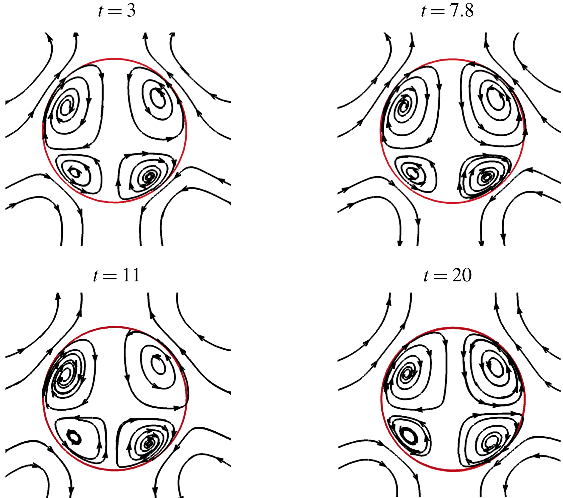
Temporal variations of streamlines in the
 $x$
–
 $z$
plane at
 $z_{CG}$
of the bubble for
 $M_{1}=0.4$
and
 $M_{2}=0.2$
. The bubble shape is shown in red. The remaining parameter values are the same as the base parameters.
(a) The surface tension (
 $\unicode[STIX]{x1D70E}$
) variation on the bubble surface (the view is in the
 $x$
–
 $z$
plane at
 $z_{CG}$
of the bubble). (b) The temperature (
 $T$
) contours on the
 $x$
–
 $z$
plane passing through the centre of gravity of the bubble. Here
 $M_{1}=0.4$
,
 $M_{2}=0.2$
and the remaining parameter values are the same as the base parameters.
Plots of (a)
 $(\unicode[STIX]{x1D70E}-\unicode[STIX]{x1D70E}_{m})/Bo$
versus
 $\unicode[STIX]{x1D703}$
and (b)
 $T-T_{m}$
versus
 $\unicode[STIX]{x1D703}$
along the equator of the bubble at
 $t=20$
for
 $M_{1}=0.4$
and
 $M_{2}=0.2$
. The remaining parameter values are the same as the base parameters.
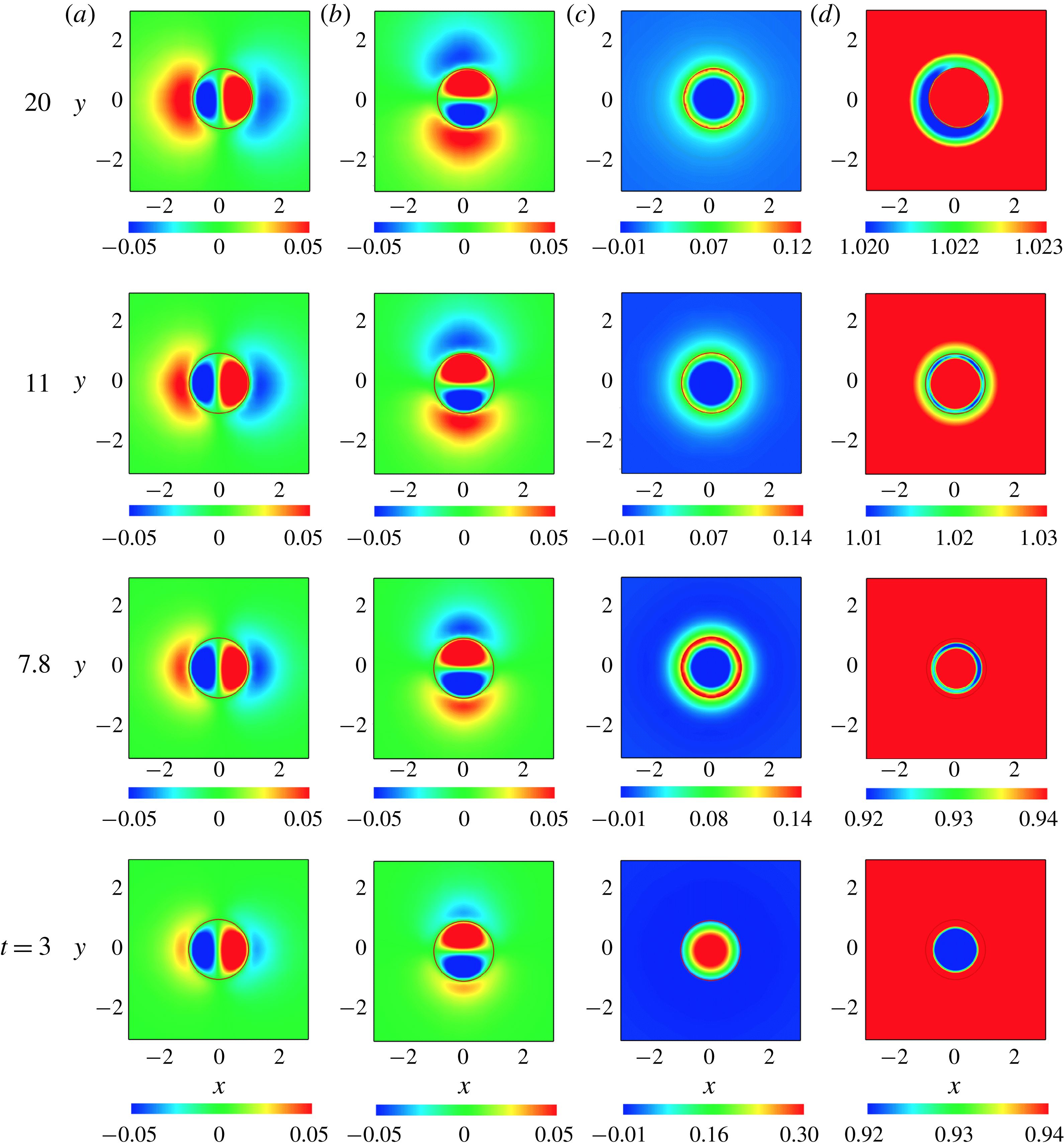
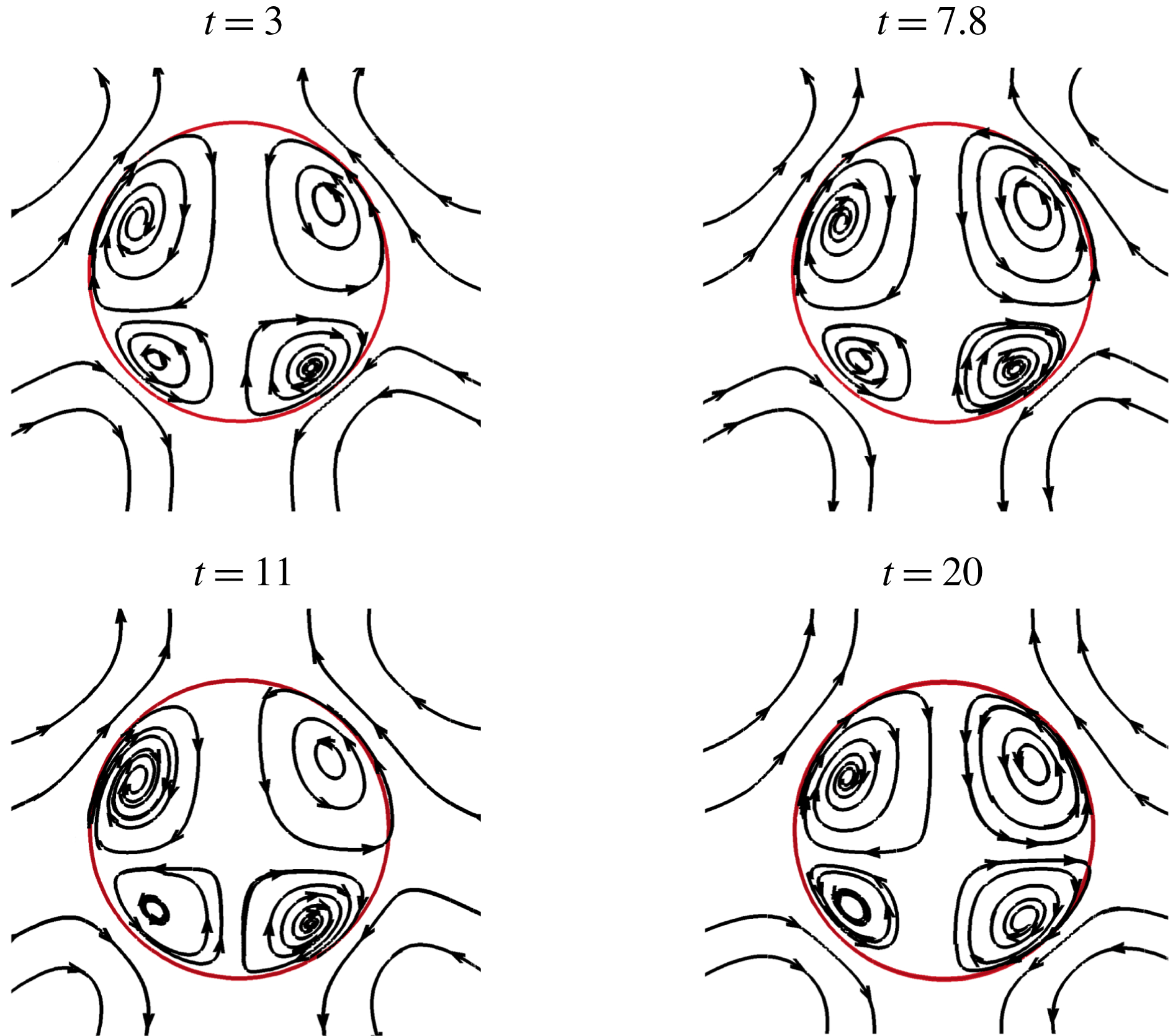
In order to rationalise this behaviour and gain further insight into the bubble dynamics, we analyse the velocity and temperature fields at various stages of the flow development for the surface-tension-dominated case, characterised by
 $Bo=10^{-3}$
. In figure 11(a–d), we show contour plots of
 $u$
,
 $v$
,
 $w$
and
 $T$
, respectively, in the
 $x$
–
 $y$
plane corresponding to
 $z=z_{CG}$
and for
 $t=3$
, 7.8, 11 and 20, which span the vertical rise and lateral migration stages (see figure 9). It can be clearly seen that, during the early stages of the flow (
 $t=3$
), motion in the vertical direction dominates the dynamics as evidenced by the magnitude of the vertical velocity component,
 $w$
, which greatly exceeds that of
 $u$
and
 $v$
; the corresponding temperature field also appears to be axisymmetric. In figure 12, we also depict the flow field in the
 $x$
–
 $z$
plane. The variation of
 $\unicode[STIX]{x1D70E}$
on the bubble surface and temperature contours in the
 $x$
–
 $z$
plane at
 $z_{CG}$
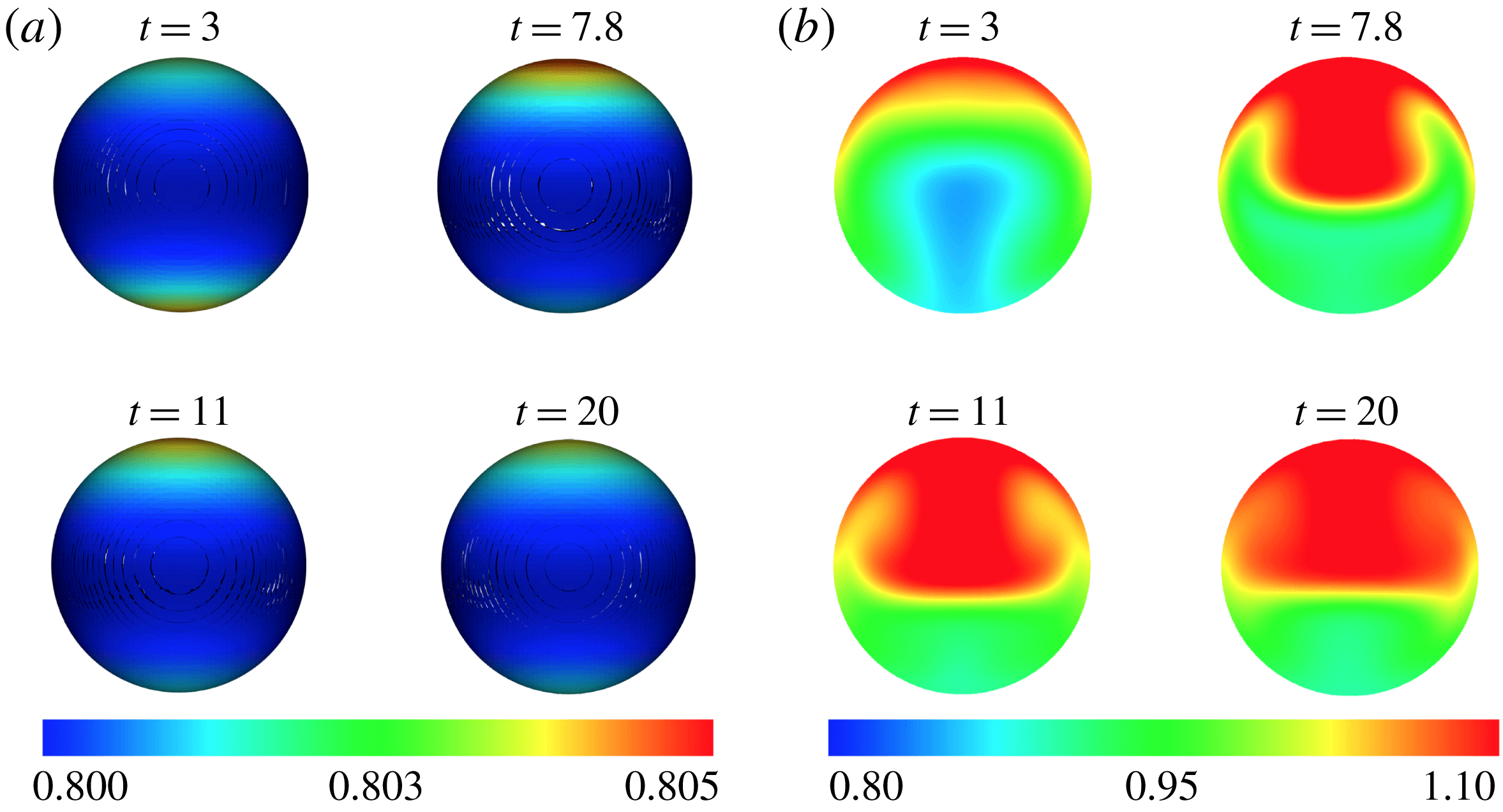
of the bubble are shown in figure 13(a,b), respectively. As shown in figure 13(a), at
 $t=3$
the bubble has just crossed
 $z=z_{m}$
with a symmetric profile of surface tension exhibiting a maximum at the bottom part of the bubble and a minimum in the middle. With increasing time (at
 $t=7.8$
), the value of
 $w$
has decreased considerably due to the Marangoni convection in the opposite direction of bubble motion as can be clearly deduced from figure 12. This is in agreement with the results illustrated in figure 9(c), which indicate that the onset of bubble departure takes places at
 $t\approx 7.8$
. Because of instability, the axisymmetry of the flow field about the
 $z$
direction breaks down at later times (see figures 11 and 12). Since the position of the bubble at
 $t=11$
is above
 $z_{m}$
, the surface tension increases with temperature and Marangoni stresses drive fluid surrounding the bubble towards the hotter regions (where surface tension is higher), pushing the bubble towards the opposite direction (see figure 13). This eventually results in driving the bubble closer to the axis of the channel, which is also reflected in figure 9; as shown in figure 9, the distance from the axis decreases for
 $t>10$
. At
 $t=20$
, as shown in figure 11(d), a markedly non-axisymmetric profile of
 $T$
arises, with the largest temperatures being in the top-right quadrant of the bubble projection on the
 $x$
–
 $y$
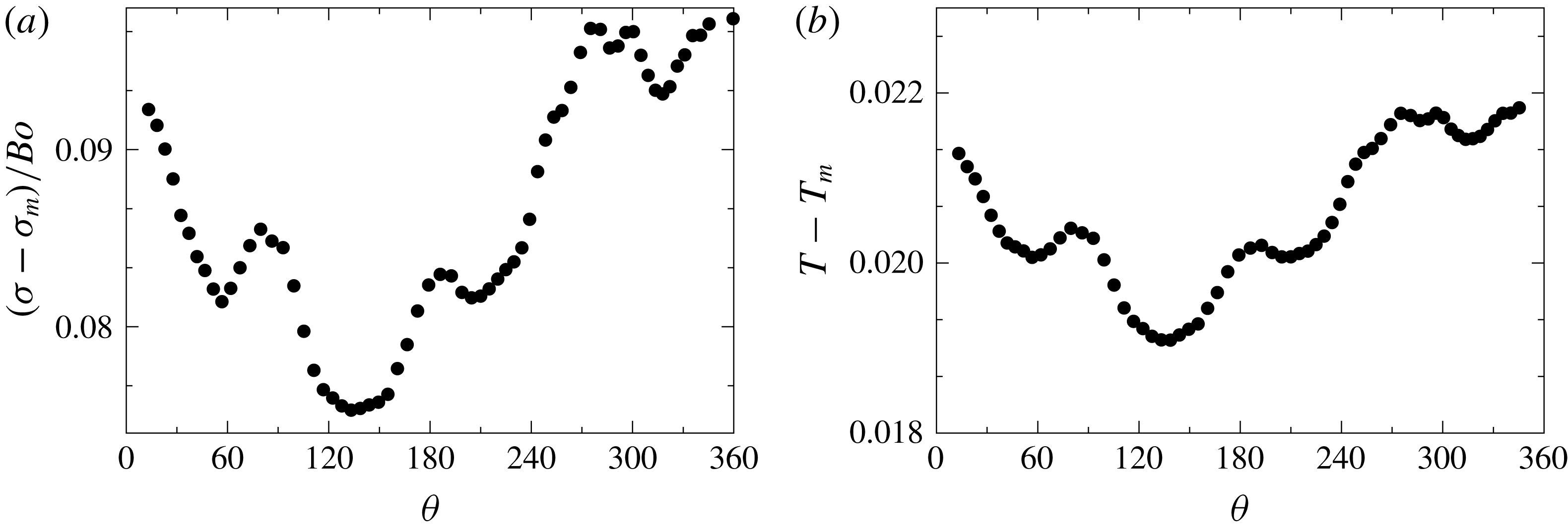
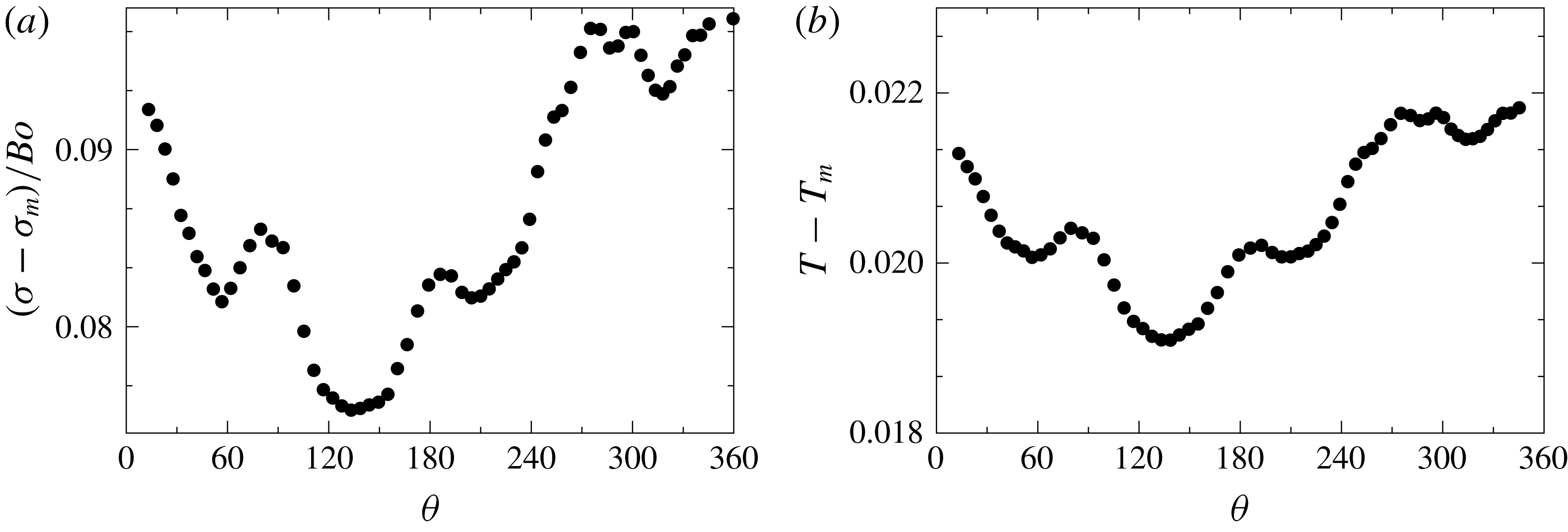
plane. At this point an asymmetry of the surface tension profile in the vertical direction becomes evident in figure 13(a). The variation of surface tension about the
 $z$
direction on the bubble surface is very small, and therefore cannot be noticed in figure 13(a) at
 $t=20$
. Thus, we plot the variation of
 $(\unicode[STIX]{x1D70E}-\unicode[STIX]{x1D70E}_{m})/Bo$
and
 $T-T_{m}$
versus
 $\unicode[STIX]{x1D703}$
along the equator of the bubble in figure 14(a,b) at
 $t=20$
. Here,
 $\unicode[STIX]{x1D703}$
is defined in the
 $x$
–
 $y$
plane and measured from the positive
 $x$
axis, and
 $\unicode[STIX]{x1D70E}_{m}$
is the minimum surface tension. The asymmetry in variations of
 $\unicode[STIX]{x1D70E}$
and
 $T$
can be clearly seen in figure 14; however, the onset of departure of the bubble from axisymmetry can be understood by performing a stability analysis.
Temporal variation of the centre of gravity of the bubble for a self-rewetting fluid (
 $M_{1}=0.4$
and
 $M_{2}=0.2$
) starting from different initial locations,
 $z_{i}$
; the location of minimum surface tension (i.e.
 $z=10$
) is shown by red dotted line. The remaining parameter values are the same as the base parameters.
Trajectories of the bubbles started from different initial locations: (a)
 $z_{i}=7.5$
, (b)
 $z_{i}=10$
and (c)
 $z_{i}=11.5$
. The rest of the parameter values are the same as those used to generate figure 15.
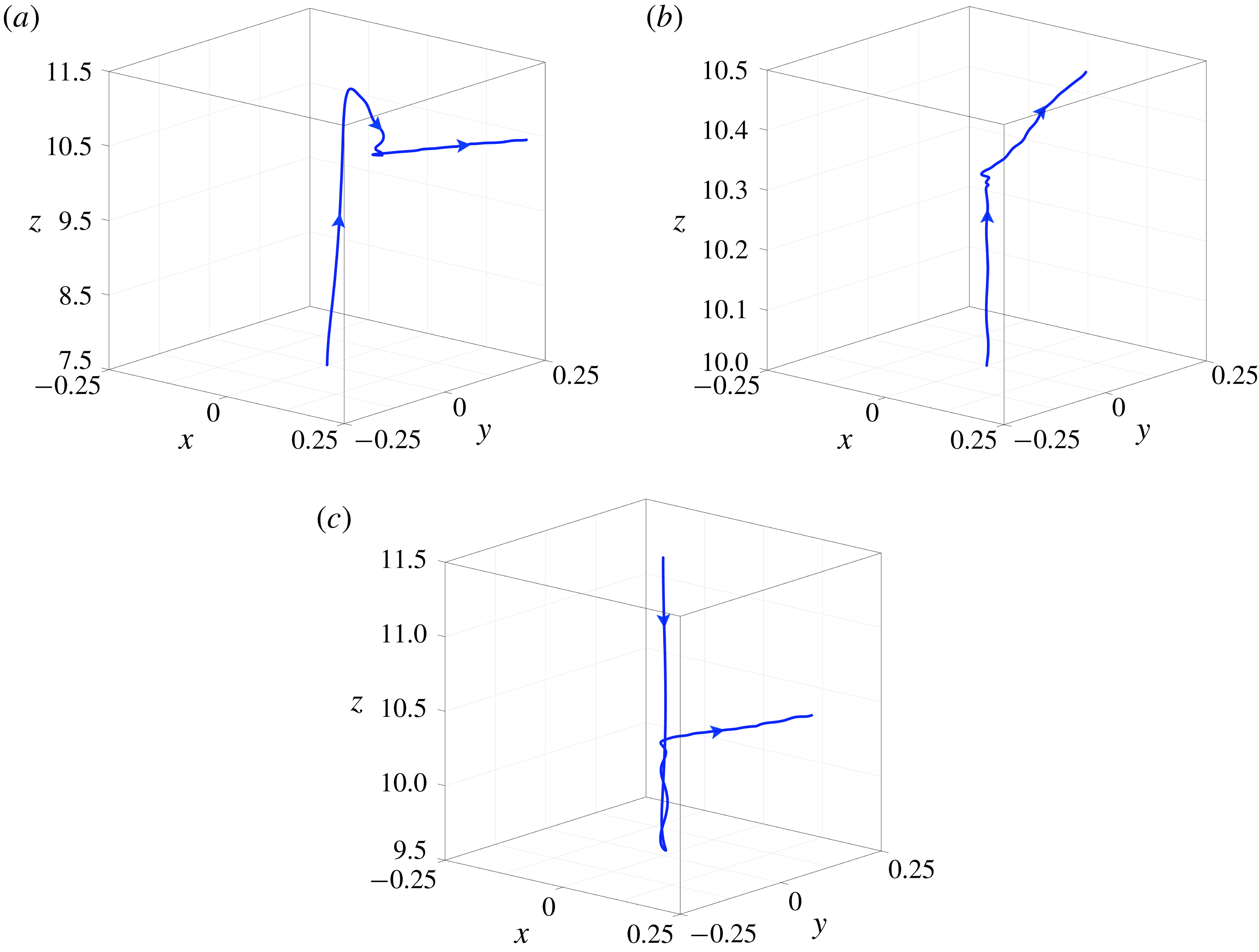
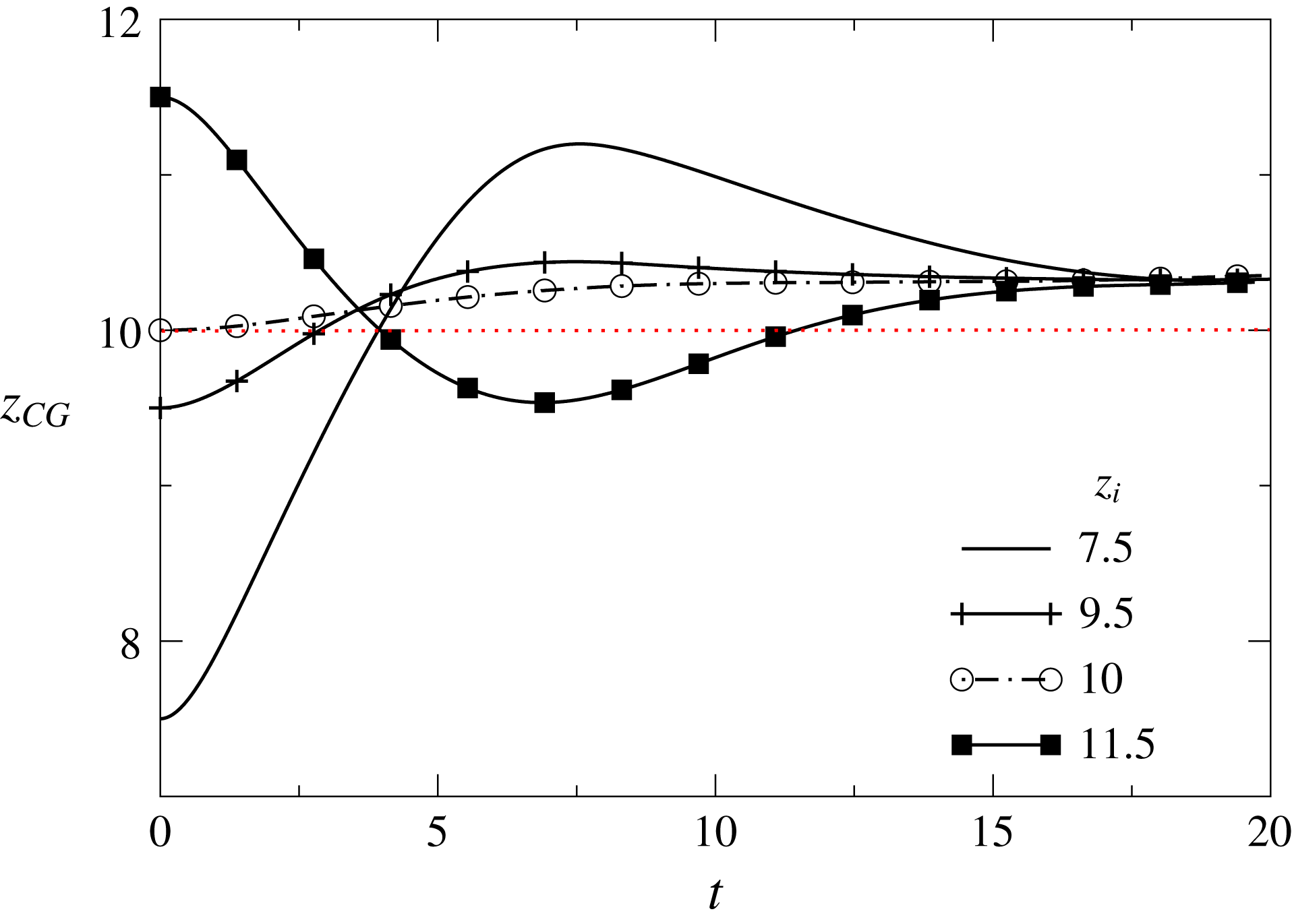
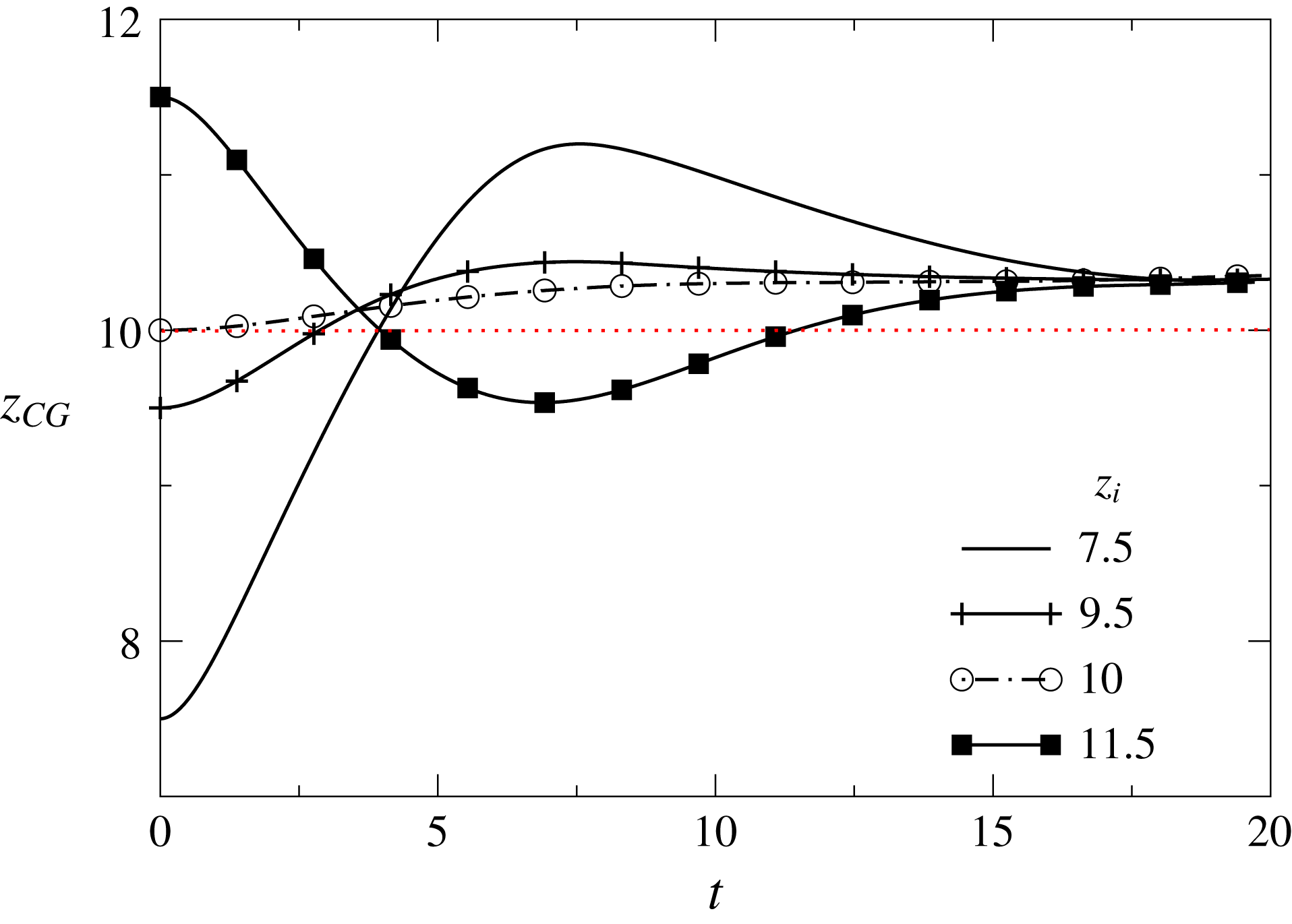
Having established the mechanism underlying the lateral migration phenomenon, we investigate next the effect of the initial location of the bubble. In figure 15, we show the evolution of the vertical position of the bubble centre of gravity as a parametric function of
 $z_{i}$
, with the remaining parameters fixed at their ‘base values’. In cases where the initial location of the bubble is lower than that associated with surface tension minimum,
 $z_{m}$
, the surface tension gradient reinforces the buoyancy-driven bubble rise. As soon as the bubble reaches elevations such that
 $z>z_{m}$
, the surface tension gradient is reversed and the bubble becomes retarded by the induced Marangoni flow. However, with increasing distance that the bubble has to cover before it reaches
 $z=z_{m}$
, it is allowed to gain momentum and thus may reach higher elevations before it eventually gets arrested. For sufficiently large values of
 $z_{i}$
, i.e.
 $z_{i}>z_{m}$
, the bubble moves in the negative
 $z$
direction under the action of Marangoni stresses whose magnitude exceeds that of the buoyancy force. In all cases, however, the terminal value of
 $z_{CG}$
is identical for all
 $z_{i}$
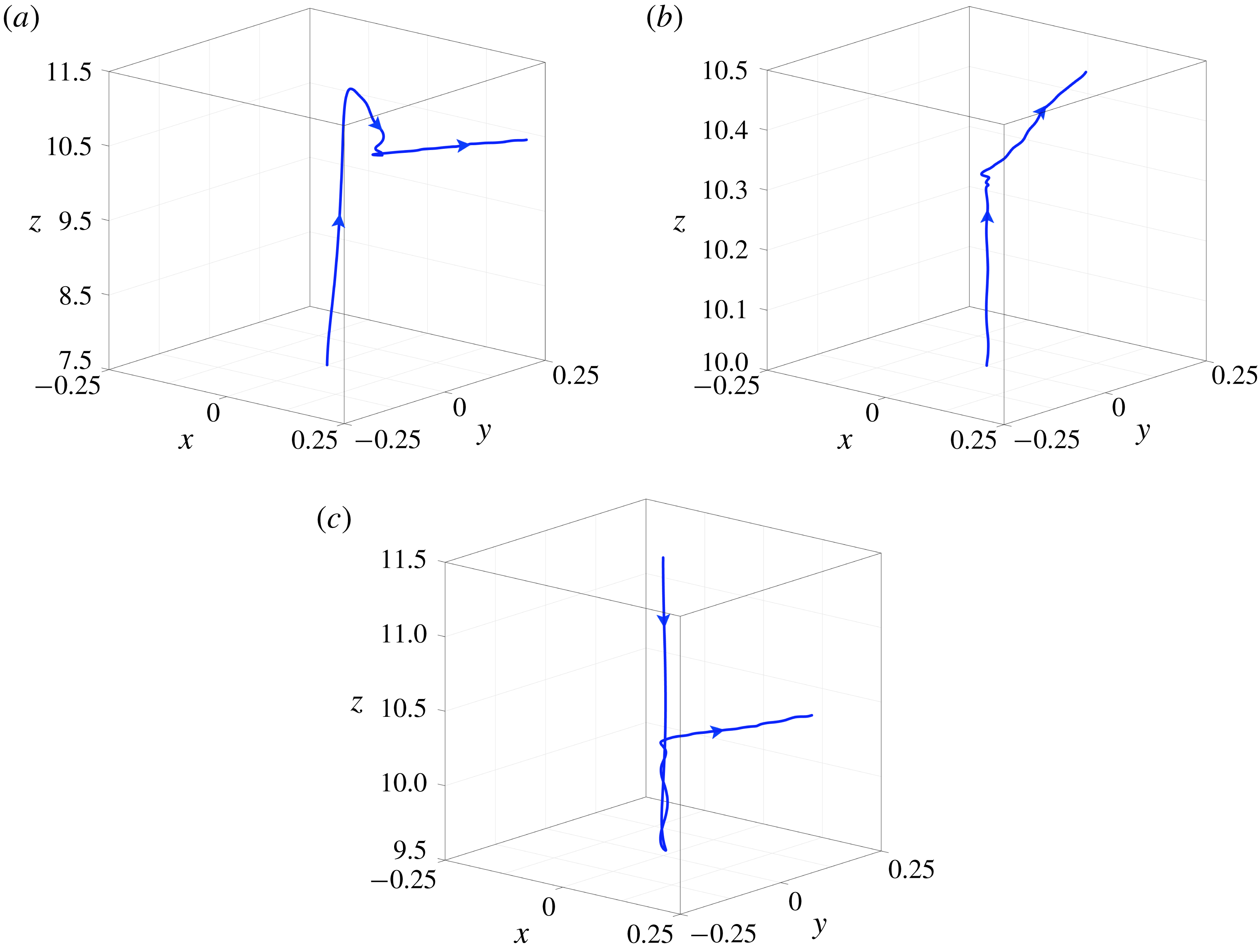
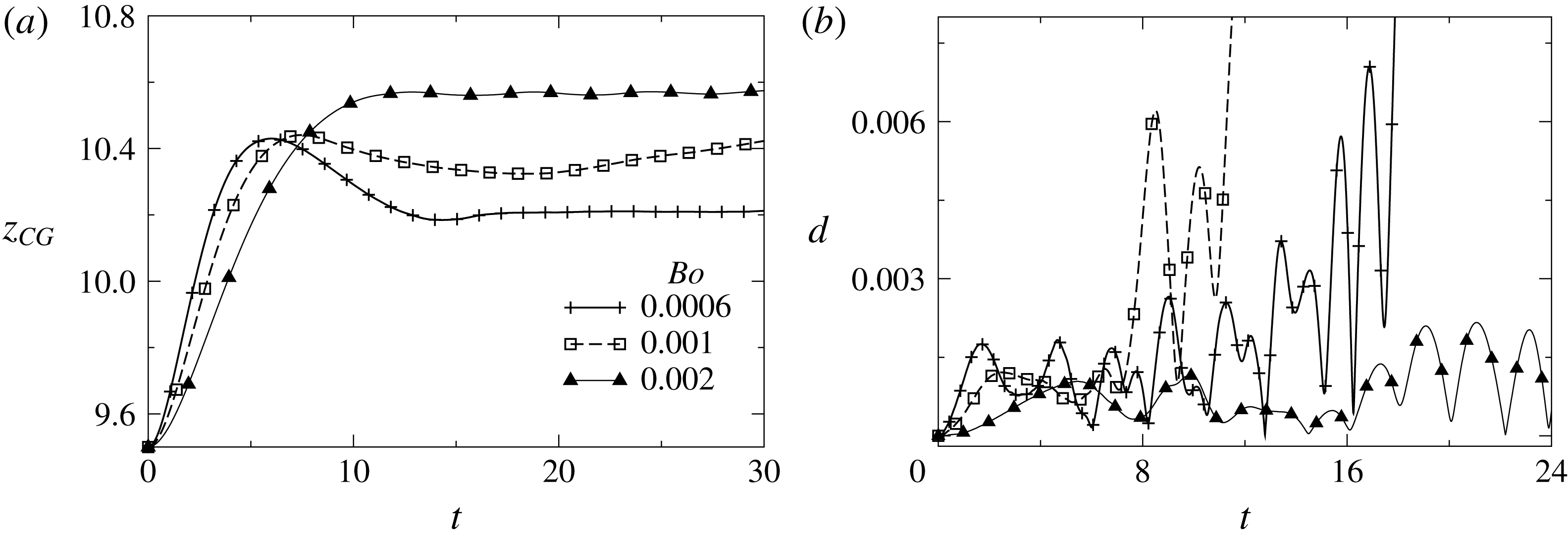
values. Moreover, even though it reaches a terminal vertical position, the bubble does not remain motionless but moves sideways as shown in figure 16.
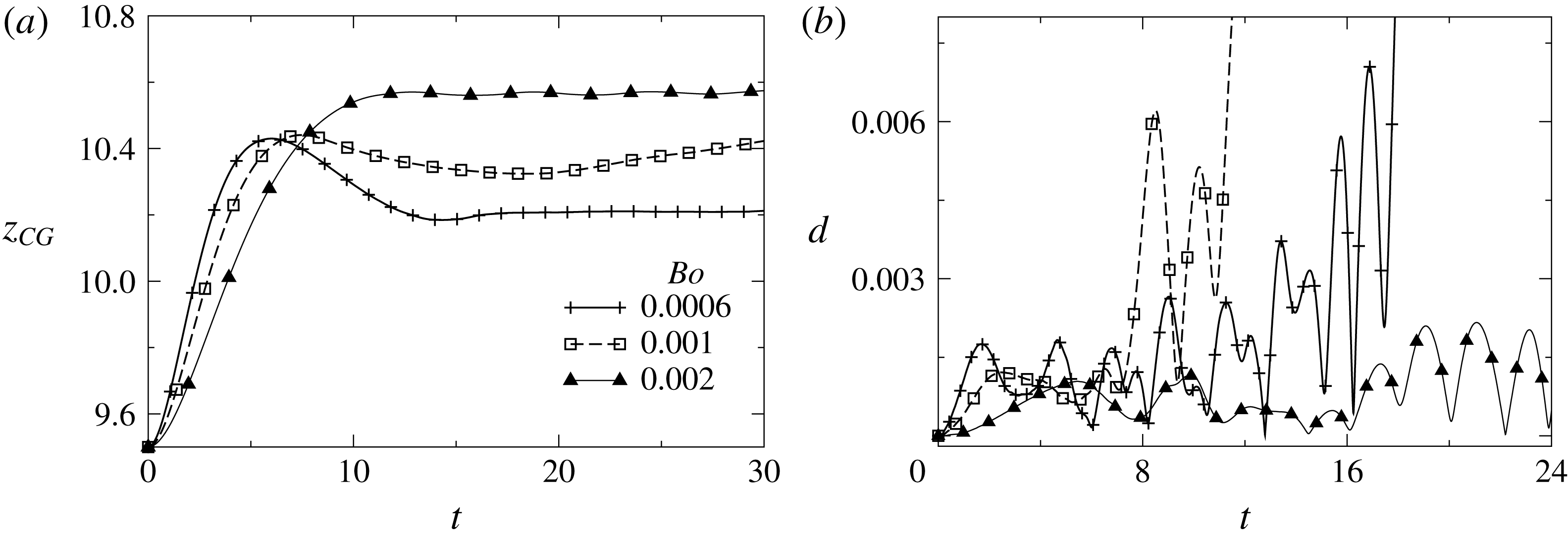
In figure 17, the temporal variation of
 $z_{CG}$
and distance from the axis,
 $d$
, are depicted for different values of the
 $Bo$
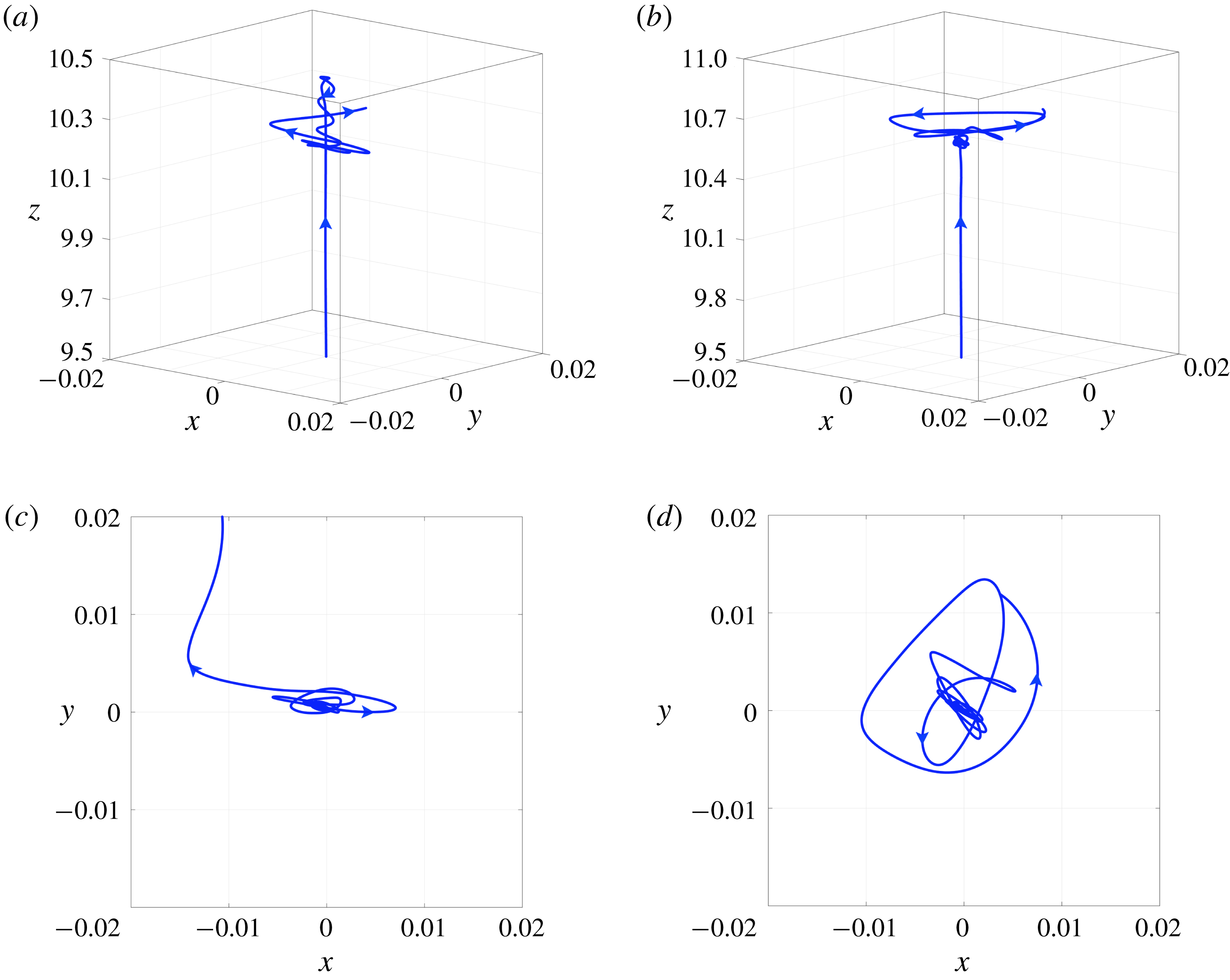
number. Moreover, in figure 18, the trajectories of the bubble for two limiting values of
 $Bo$
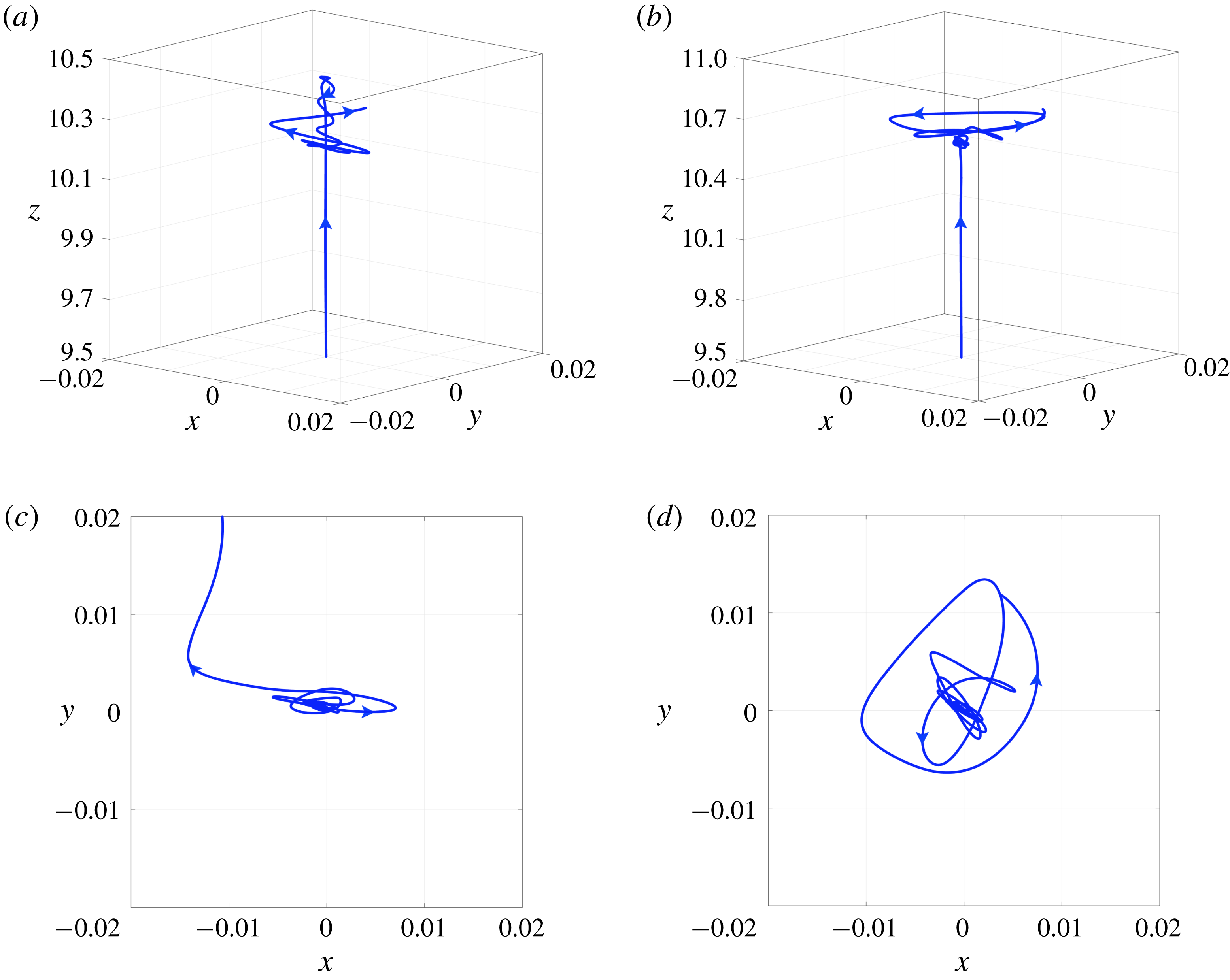
are depicted in two different projections. As shown in figures 17 and 18, the three-dimensional effects on the flow become less pronounced with increasing value of
 $Bo$
, while the onset of lateral migration takes place at later times, e.g. see figure 18(c). This is indeed a striking difference from the case of a bubble rising under isothermal conditions, for which it is believed that asymmetrical deformation of the bubble is associated with path instability (Tripathi et al.
Reference Tripathi, Sahu and Govindarajan2015a
; Sharaf et al.
Reference Sharaf, Premlata, Tripathi, Karri and Sahu2017). This is clearly not the case for the present system where the path instability is actually due to the interplay of inertia and thermocapillarity, and appears to be favoured by bubbles that retain their spherical shape. The aspect ratio of the bubble (ratio of the diameters of the bubble along any two axes) for the parameters considered is approximately one all the times, i.e. the bubbles remain mostly spherical. In addition to the mechanism of the lateral migration discussed above (see figure 11), a stability analysis similar to those performed by Magnaudet & Mougin (Reference Magnaudet and Mougin2007), Yang & Prosperetti (Reference Yang and Prosperetti2007), Zenit & Magnaudet (Reference Zenit and Magnaudet2008) and Cano-Lozano et al. (Reference Cano-Lozano, Tchoufag, Magnaudet and Martínez-Bazán2016) for isothermal systems may also provide further insight into this phenomenon.
Temporal variation of (a) the centre of gravity of the bubble, and (b) the distance of the centre of gravity of the bubble from the axis (
 $d=(x_{CG}^{2}+y_{CG}^{2})^{1/2}$
) for different values of
 $Bo$
. The remaining parameter values are the same as the base parameters.
Trajectories of the bubble. (a,b) Three-dimensional view, and (c,d) top view (projection on the
 $x$
–
 $y$
plane) for (a,c)
 $Bo=6\times 10^{-4}$
and (b,d)
 $Bo=2\times 10^{-3}$
. The rest of the parameter values are the same as those used to generate figure 17.
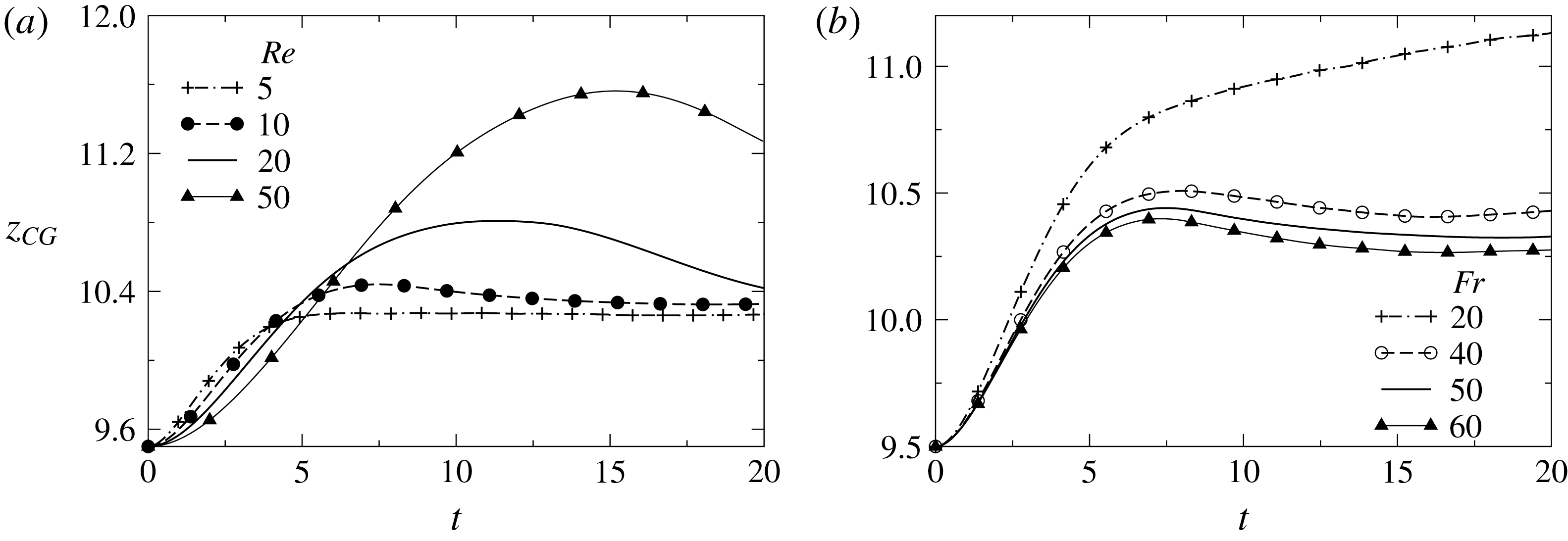
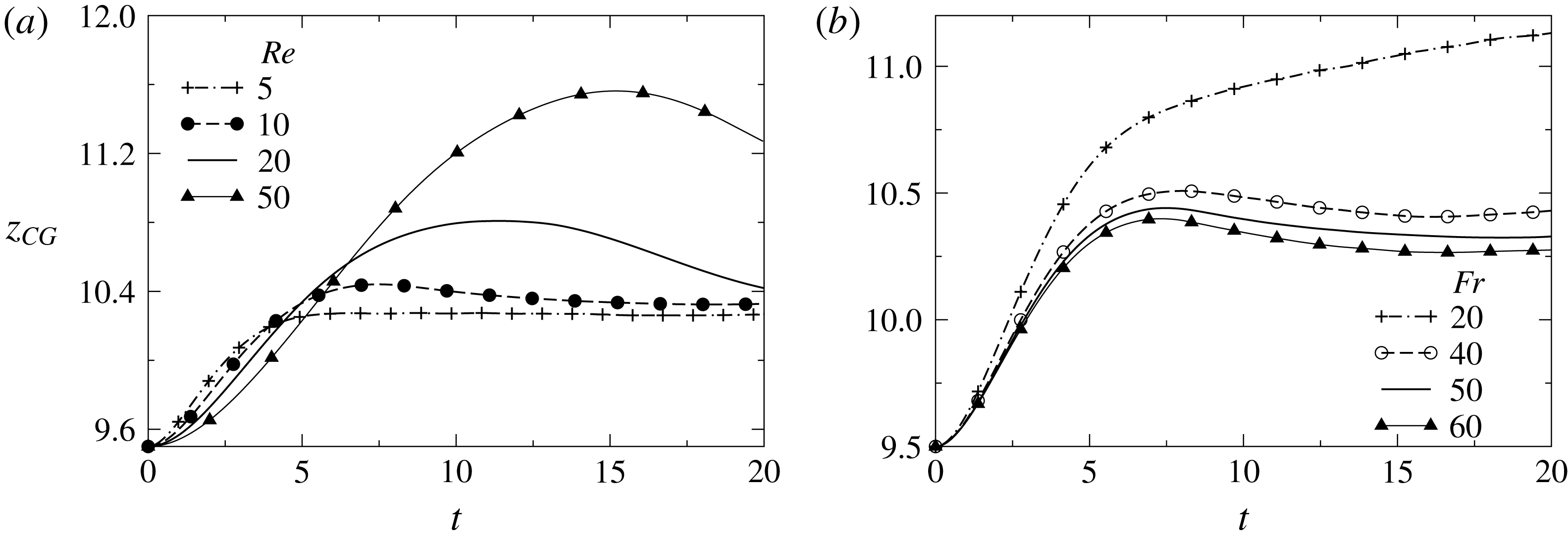
Effect of (a) Reynolds number for
 $Fr=50$
and (b) Froude number for
 $Re=10$
on the temporal variation of the centre of gravity of the bubble. The remaining parameter values are the same as the base parameters.
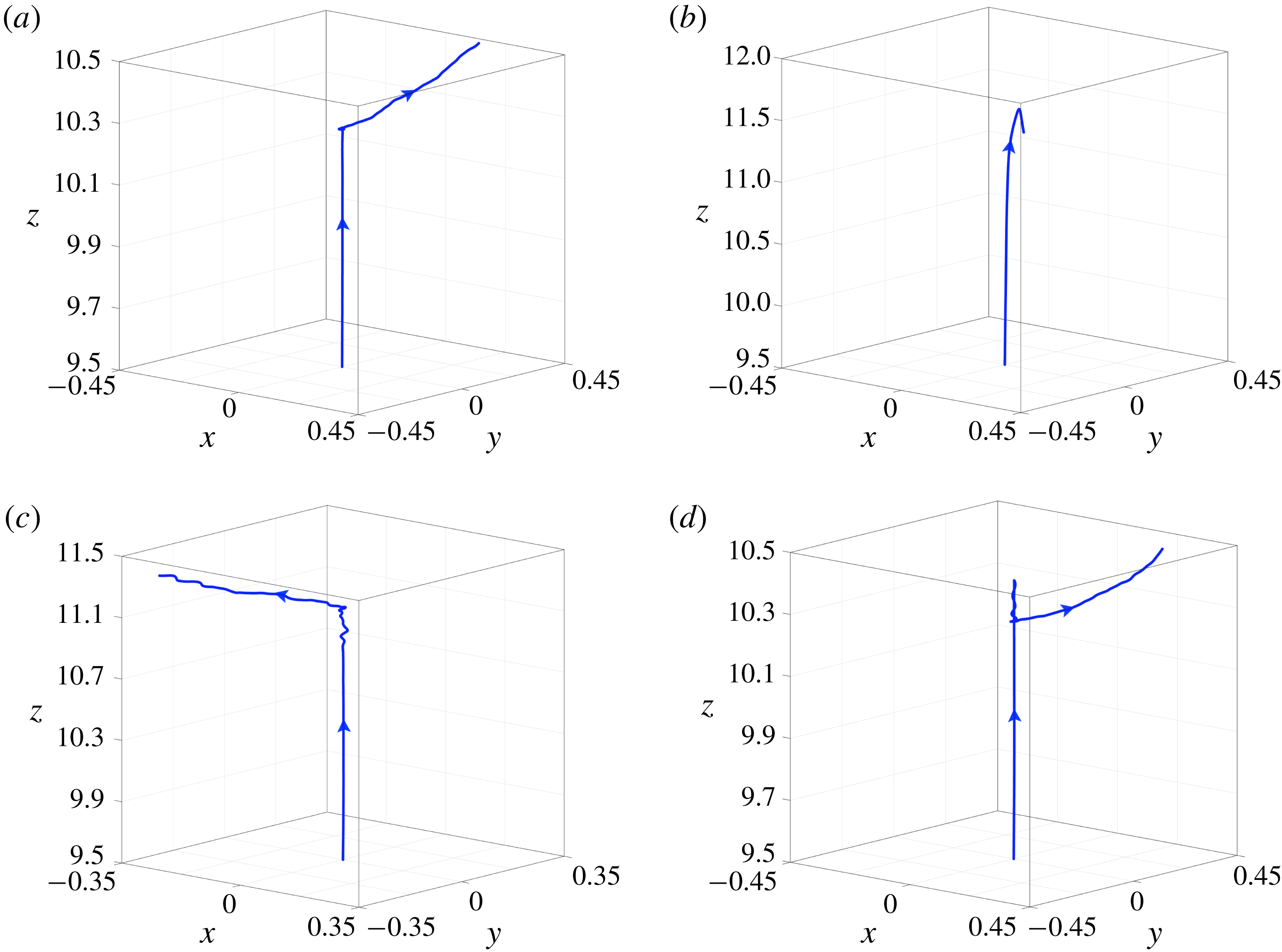
Trajectories of the bubble for (a)
 $Re=5$
and (b)
 $Re=50$
for
 $Fr=50$
, and (c)
 $Fr=20$
and (d)
 $Fr=60$
for
 $Re=10$
. The rest of the parameter values are the same as those used to generate figure 19.
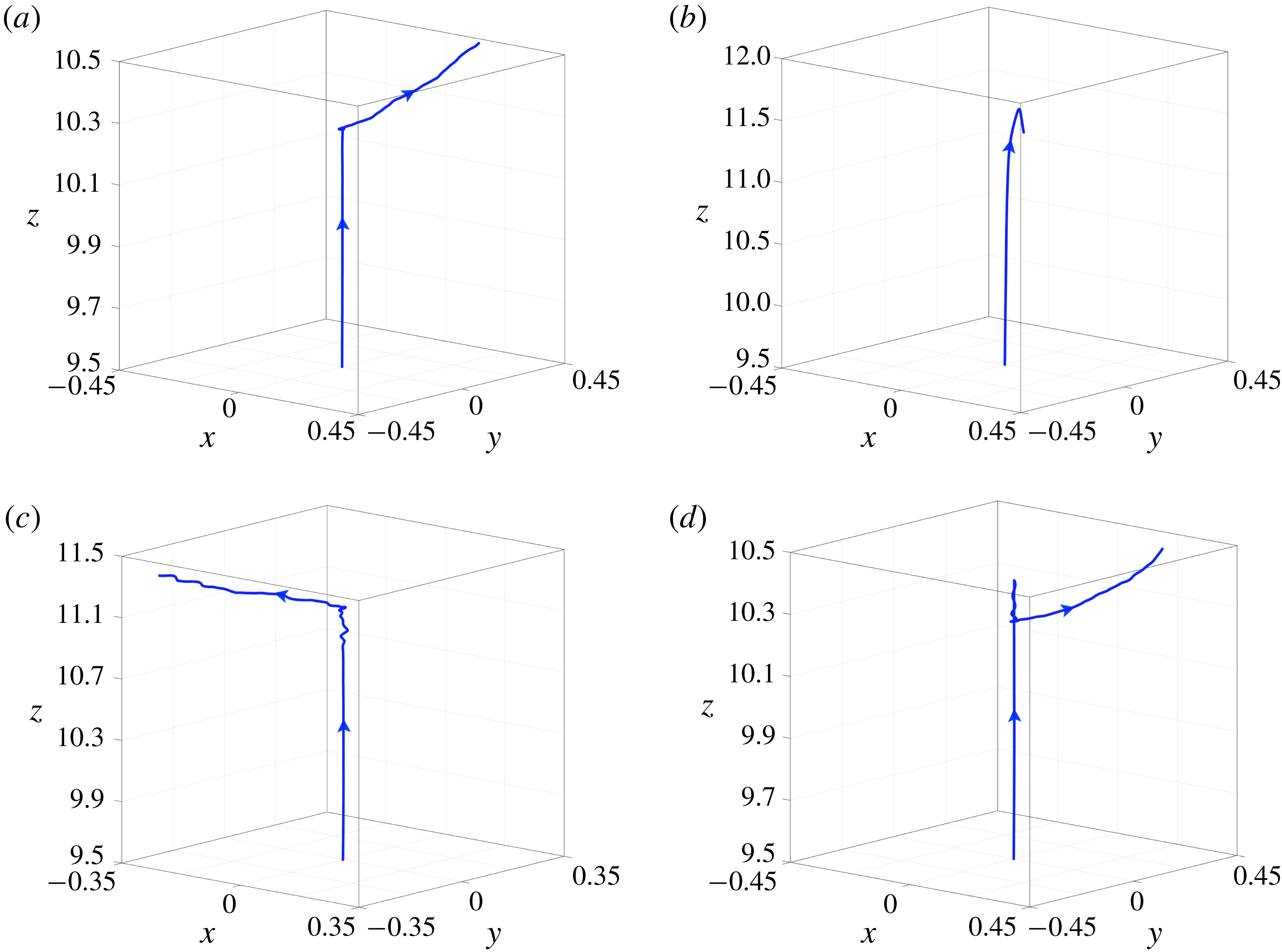
The temporal variations of
 $z_{CG}$
for different values of Reynolds number and Froude number are plotted in figures 19(a) and 19(b), respectively. It can be seen in figure 19(a) that, with the increase in the value of Reynolds number and keeping the Froude number fixed at
 $Fr=50$
, the bubble reaches higher maximum elevations due to the increased effect of inertia. The latter also has an important implication on the level of thermocapillary stresses that the bubble experiences. Owing to our assumption of quadratic dependence of surface tension on temperature, the induced Marangoni stresses become stronger as we move further away from the location associated with surface tension minimum,
 $z_{m}$
; this can be clearly seen in figure 1(b). According to the previous discussion, since Marangoni stresses can be held responsible for the breakdown of symmetry, it is reasonable to expect that if the bubble is allowed to reach higher elevations then it should be more susceptible to three-dimensional effects. Our simulations indicate that this is indeed the case, and inspection of figure 20(a,b) reveals that increasing
 $Re$
for a fixed
 $Fr$
leads to enhanced lateral migration. On the other hand, increasing Froude number by keeping the Reynolds number fixed at
 $Re=10$
, thereby reducing the effect of buoyancy as compared to Marangoni stresses, decreases the rise speed of the bubble and brings down the location of the bubble arrest. For low values of
 $Fr$
the bubble has not reached a terminal vertical position even at late times, due to the stronger effect of buoyancy, and exhibits a low-amplitude zig-zag motion as it rises slowly (see figure 20
c). For higher values of
 $Fr$
, the corresponding effect of Marangoni stresses becomes more important (the characteristic velocity is based on Marangoni scaling) and lateral migration of the bubble is enhanced (see figure 20
d).
5 Concluding remarks
The rise dynamics of a gas bubble in a square channel filled with a ‘self-rewetting’ fluid whose surface tension exhibits a parabolic dependence on temperature with a well-defined minimum is investigated numerically. A linearly increasing temperature in the vertical direction is imposed at the sidewalls of the channel. A modified open-source finite-volume VoF-based multiphase flow solver, Basilisk (originally developed by Popinet and co-workers), wherein we include the tangential gradient of surface tension force (known as Marangoni or thermocapillary force) has been used in the present study. It is very challenging to accurately calculate the tangential force term operating at the interface in the VoF framework. Thus, extensive validation exercises were performed by comparing the results obtained using the present solver with the previous experimental, theoretical and computational studies.
The main objectives of the present study are as follows: (i) to investigate the effect of Marangoni stresses on bubble rise dynamics in a self-rewetting fluid using a consistent model fully accounting for the tangential surface tension forces; and (ii) to highlight the effects of three-dimensionality on the bubble rise dynamics. In the case of isothermal and non-isothermal systems with ‘linear’ fluid (whose surface tension decreases linearly with increasing temperature), the bubble moves in the upward direction in an almost vertical path as shown in figure 8(a). On the other hand, the behaviour observed in the case of the self-rewetting fluid is strikingly different. Our results indicate that in a self-rewetting fluid, as the bubble crosses the location of minimum surface tension, the buoyancy-induced upward motion of the bubble is retarded by a thermocapillary-driven flow acting in the opposite direction, which in some situations outweighs buoyancy, which in turn leads to the migration of the bubble in the downward direction. In the later stages of this downward motion, as the bubble reaches its position of arrest, the vertical motion decelerates. In the presence of small disturbances, which in our simulations can be simply introduced due to the presence of small numerical errors, the flow becomes unstable and the bubble experiences an asymmetrical temperature distribution as it moves away from the axis of symmetry, which ultimately leads to the bubble migration towards one of the channel walls as shown in figure 8(b).
These phenomena are observed at sufficiently small Bond numbers. In the case of stronger self-rewetting behaviour (
 $M_{1}=0.6$
; see figure 10), the bubble undergoes spiralling motion. The mechanisms underlying these three-dimensional effects are elucidated by considering how the surface tension dependence on temperature affects the thermocapillary stresses in the flow. It is shown that the Marangoni stresses can be held responsible for the breakdown of symmetry, and it is reasonable to expect that if the bubble is allowed to reach higher elevations then it should be more susceptible to three-dimensional effects. This is indeed a striking difference with the case of a bubble rising under an isothermal condition, for which it is known that bubble deformability is actually a necessary condition for path instability (Tripathi et al.
Reference Tripathi, Sahu and Govindarajan2015a
). This is clearly not the case for the present system, where the path instability is actually due to the interplay of inertia and thermocapillarity, and appears to be favoured by bubbles that retain their spherical shape.
Our study on the effect of the initial location of the bubble rising in a self-rewetting fluid for low inertia also shows that, irrespective of the different starting vertical positions (i.e. above or below the location of minimum surface tension), for the same set of the rest of the dimensionless parameters, the bubble gets arrested at a particular
 $z$
location, which almost coincides with the prediction from the theoretical analysis in the Stokes flow regime. The effects of other dimensionless numbers, such as Reynolds and Froude numbers, are also investigated. It is observed that increasing Reynolds number or decreasing Froude number, keeping the other parameters fixed, has a similar effect.
Acknowledgements
K.C.S. thanks the Indian National Science Academy for their financial support. M.K.T. also thanks the Department of Science and Technology, India (project no. DST/EES/2015037) for financial support. We sincerely thank the anonymous reviewers for their many insightful comments and suggestions.