1 Introduction
The dynamics of geophysical flows in the oceans and the atmosphere is dominated by both the Earth’s rotation and fluid stratification (Pedlosky Reference Pedlosky1987). For sufficiently slow motions with respect to the rotation period, the flow consists of vertical columns aligned with local gravity, so the flow is essentially two-dimensional (2-D). Barotropic models have been used as a first approximation to represent some of the most paradigmatic oceanic and atmospheric flows, such as the ocean wind-driven circulation in a closed basin (Stommel Reference Stommel1948), or the
 $\unicode[STIX]{x1D6FD}$
-drift of cyclonic vortices in the atmosphere (Adem Reference Adem1956). The motion of a barotropic fluid admits spatial variations of the solid bottom (Grimshaw, Tang & Broutman Reference Grimshaw, Tang and Broutman1994). With variable topography the flow still moves in a columnar fashion, but now under stretching and squeezing effects as columns transit from deep to shallow regions or vice versa. The dynamics of geophysical flows may be studied using laboratory experiments with homogeneous fluids in a rotating container (van Heijst & Clercx Reference van Heijst and Clercx2009). In particular, experiments with flows over variable topography are often performed to investigate the behaviour of vortices, jets and quasi-2-D turbulence in rapidly rotating systems (Zavala Sansón & van Heijst Reference Zavala Sansón, van Heijst, von Larcher and Williams2014).
A substantial limitation of barotropic dynamics to model geophysical systems is the stiffness of fluid columns, a characteristic that does not hold for atmospheric and oceanic flows because of vertical stratification. An intermediate, 2-D barotropic formulation that mimics the vertical structure of a stratified flow was derived by Charney (Reference Charney1949) in the atmospheric context. The model consists of assuming a baroclinic atmosphere whose horizontal motion at different vertical levels varies in magnitude but not in direction, according to a pre-defined vertical structure. Charney justified such a strong dynamical constraint by noticing that horizontal isobars and isotherms in the atmosphere nearly coincide and that large-scale winds maintain their direction at different heights. The dynamical equations at an intermediate level (determined by the average of the vertical structure) were shown to have an approximate form identical to the equations for an ‘equivalent-barotropic’ atmosphere using the variables at that level. Thus, solving the equivalent-barotropic system was equivalent to solving the baroclinic flow at the intermediate level.
The concept of an equivalent-barotropic flow was not used in the oceanographic context until decades later. Killworth (Reference Killworth1992) reported that the Antarctic circumpolar current (ACC) might be approximated as an equivalent-barotropic structure, that is, a flow whose velocity decreases with depth while maintaining the same direction. Gille (Reference Gille1995) proposed an exponential structure function
 $\text{e}^{z/z_{0}}$
, where
 $z$
is the vertical direction and
 $z_{0}$
a reference
 $e$
-folding depth. Using a large number of autonomous mid-depth (900 m) drifters, Gille (Reference Gille2003) confirmed the equivalent-barotropic character of the ACC with an
 $e$
-folding depth of 700 m. One of the few other regions where an equivalent-barotropic structure is documented is in the southern Gulf of Mexico. Perez-Brunius et al. (Reference Perez-Brunius, García-Carrillo, Dubranna, Sheinbaum and Candela2013) measured the surface and deep circulation at the Bay of Campeche (located at the south-western part of the basin), using surface drifters and current meter moorings at depths of up to 2000 m during several months. One of the main circulation features was a semi-permanent cyclonic gyre. By mean of empirical orthogonal functions, the authors found that the decreasing circulation at different depths maintained the same direction, approximately, with an estimated
 $e$
-folding depth of 650 m. Another example was reported in the Caspian Sea (Ghaffari, Isachsen & LaCasce Reference Ghaffari, Isachsen and LaCasce2013).
The equivalent-barotropic approach is based on the large-scale, linear geostrophic dynamics (Killworth Reference Killworth1992). Consequently, model studies are focused on the steady, linear problem. Krupitsky et al. (Reference Krupitsky, Kamenkovich, Naik and Cane1996) derived a model for a stationary, linear ACC in the presence of wind forcing and bottom friction. A detailed account of several linear models to study this oceanic system was reported by LaCasce & Isachsen (Reference LaCasce and Isachsen2010). However, nonlinear effects might play an important role in, for instance, western boundary currents or flows with strong curvature (Hughes & De Cuevas Reference Hughes and De Cuevas2001). Also, it is well known that nonlinear effects provide the self-propelling propagation mechanism of intense vortices and prevent their dispersive decay as they drift on a
 $\unicode[STIX]{x1D6FD}$
-plane (Sutyrin Reference Sutyrin1994) or over a topographic slope in laboratory experiments (Flór & Eames Reference Flór and Eames2002). Regarding the ACC, Hughes (Reference Hughes2005) proposed that nonlinear terms should be taken into account to understand the topographic effects on the ACC better. That author concluded that the advection of relative vorticity in the meandering motions of the current is part of the near-surface vorticity balance.
In this paper, a time-dependent, nonlinear formulation of an equivalent-barotropic flow over bottom topography is analysed. Forcing and dissipative terms are considered as well. The vertical structure function is exponential, although the model accepts arbitrary functions subject to some basic conditions. The inclusion of nonlinear effects necessarily restricts the model validity because the assumption of a pre-defined vertical structure is incompatible with the quadratic form of advective terms. Nevertheless, the barotropic assumption is still reasonable when the vertical structure is not abrupt. The advantages and limitations are discussed.
To test the model, numerical simulations of three flow systems with bottom topography are performed. In the first example, we explore the behaviour of cyclonic vortices in the presence of a submarine mountain. The purpose is to examine the nonlinear vortex drift induced by the topographic feature depending on the vertical structure of the flow. This problem was studied for a homogeneous flow through laboratory experiments and simulations by Zavala Sansón, Barbosa Aguiar & van Heijst (Reference Zavala Sansón, Barbosa Aguiar and van Heijst2012). Such experimental observations serve as a reference to evaluate the modification of nonlinear effects on the translating vortex. The second example is the wind-driven oceanic flow in a closed basin with topography. It is the classical Stommel problem (Stommel Reference Stommel1948), but now considering a non-flat bottom and the equivalent-barotropic dynamics. It is found that the steady balance that characterises the Stommel problem is not reached when the vertical structure decays rapidly, thus decreasing the effects of the topography and enhancing the wind forcing. A third example concerns the wind-driven circulation in the western Gulf of Mexico, which is simulated by using realistic bottom topography and a simplified, climatological wind field. We explore the formation of the Campeche cyclone mentioned above under the equivalent-barotropic dynamics. In contrast to the Stommel problem, we can compare the results, at least qualitatively, with oceanographic observations.
The paper is organised as follows. In § 2 we revisit the equivalent-barotropic model and present the nonlinear, time-dependent vorticity equation. Section 3 is devoted to examining numerical solutions of cyclonic vortices in the presence of a submerged circular mountain. In § 4 we present simulations of the Stommel problem with topography. In § 5, the conditions for the formation of the Campeche gyre are analysed. Finally, in § 6 the results are summarised and discussed.
2 Equivalent-barotropic dynamics
The present derivation follows several steps and assumptions made in previous studies, mainly those reported by Gille (Reference Gille1995), Krupitsky et al. (Reference Krupitsky, Kamenkovich, Naik and Cane1996) and LaCasce & Isachsen (Reference LaCasce and Isachsen2010). The aim is to justify the inclusion of the time derivative and nonlinear terms in the vorticity equation and to identify the associated error. Also, the procedure allows the use of different forms of the vertical structure of the flow and considers the vertical advection of vorticity.
2.1 Flow with vertical structure
Consider a barotropic flow under the
 $\unicode[STIX]{x1D6FD}$
-plane approximation in a coordinate system
 $(x,y,z)$
(with zonal, meridional and vertical directions, respectively). The planetary vorticity is
 $f=f_{0}+\unicode[STIX]{x1D6FD}y$
, where
 $f_{0}$
is the Coriolis parameter at a reference latitude (chosen as
 $y=0$
), and
 $\unicode[STIX]{x1D6FD}$
its latitudinal variation. The solid bottom is space dependent, so the fluid depth is
 $h(x,y)$
, which is time independent under the rigid-lid approximation. The vertical coordinate is
 $z=0$
at the surface and
 $z=-h$
at the bottom.
The horizontal velocity
 $\boldsymbol{v}$
and the pressure
 $p$
are assumed to have a separable form
 $$\begin{eqnarray}\displaystyle \left.\begin{array}{@{}c@{}}\displaystyle \boldsymbol{v}(x,y,z,t)=P(z)\boldsymbol{v}_{s}(x,y,t),\\ p(x,y,z,t)=P(z)p_{s}(x,y,t),\end{array}\right\} & & \displaystyle\end{eqnarray}$$
where the subindex
 $s$
indicates the variables evaluated at the surface and
 $P(z)$
is the dimensionless structure function in the vertical direction. The full 3-D velocity vector is
 $(u,v,w)=(Pu_{s},Pv_{s},w)$
with
 $w(x,y,z,t)$
the vertical component. The function
 $P(z)$
is required to satisfy the following conditions:
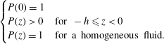 $$\begin{eqnarray}\displaystyle \left\{\begin{array}{@{}ll@{}}\displaystyle P(0)=1\quad & \\ \displaystyle P(z)>0\quad & \text{for }-h\leqslant z<0\\ \displaystyle P(z)=1\quad & \text{for a homogeneous fluid.}\end{array}\right. & & \displaystyle\end{eqnarray}$$
The first condition ensures that the surface values are recovered at
 $z=0$
. The second one avoids flow reversal through the fluid depth, which is a physical but not a mathematical restriction. The third condition states that a homogeneous flow does not have a vertical structure.
2.2 Equivalent depth and velocity components
Given
 $P(z)$
, the following vertical scales are calculated
 $$\begin{eqnarray}F(x,y)=\int _{-h}^{0}P(z)\,\text{d}z,\quad G(x,y)=\int _{-h}^{0}P^{2}(z)\,\text{d}z.\end{eqnarray}$$
The vertical average of the vertical structure,
 $F$
, is defined as the equivalent depth. If the fluid is homogeneous (
 $P=1$
), then both
 $F$
and
 $G$
are the same as the fluid depth,
 $F=G=h$
.
The fluid is incompressible, so the continuity equation is
 $\unicode[STIX]{x1D735}\boldsymbol{\cdot }(Pu_{s},Pv_{s},w)=0$
. Integrating from
 $-h$
to 0 (using the kinematic conditions at the surface
 $w(0)=0$
and at the bottom
 $w(-h)=\boldsymbol{v}(-h)\boldsymbol{\cdot }\unicode[STIX]{x1D735}(-h)$
) yields
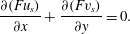 $$\begin{eqnarray}\frac{\unicode[STIX]{x2202}(Fu_{s})}{\unicode[STIX]{x2202}x}+\frac{\unicode[STIX]{x2202}(Fv_{s})}{\unicode[STIX]{x2202}y}=0.\end{eqnarray}$$
The Leibnitz rule was used to find that the vertical velocity at the bottom is
 $w(-h)=-\boldsymbol{v}_{s}\boldsymbol{\cdot }\unicode[STIX]{x1D735}F$
. Continuity (2.4) allows the introduction of a transport function
 $\unicode[STIX]{x1D713}(x,y,t)$
, such that the surface horizontal velocities are
 $$\begin{eqnarray}u_{s}=\frac{1}{F}\frac{\unicode[STIX]{x2202}\unicode[STIX]{x1D713}}{\unicode[STIX]{x2202}y},\quad v_{s}=-\frac{1}{F}\frac{\unicode[STIX]{x2202}\unicode[STIX]{x1D713}}{\unicode[STIX]{x2202}x}.\end{eqnarray}$$
The vertical velocity
 $w$
can be derived by integrating the continuity equation again, but now from an arbitrary level
 $z$
to the surface
 $z=0$
(or, equivalently, from
 $-h$
to
 $z$
),
 $$\begin{eqnarray}w(x,y,z,t)=\left(\int _{z}^{0}P(z^{\prime })\,\text{d}z^{\prime }\right)\unicode[STIX]{x1D735}\boldsymbol{\cdot }\boldsymbol{v}_{s}.\end{eqnarray}$$
Note that
 $w$
is separable also: the
 $x,y$
-dependence is given by the horizontal divergence of the surface flow, while the
 $z$
-dependence is given by the integral of
 $P(z)$
. For a purely barotropic flow with uniform horizontal velocity
 $(u,v)=(u_{s},v_{s})$
, the vertical component is linear in
 $z$
,
 $$\begin{eqnarray}w(x,y,z,t)=-z\unicode[STIX]{x1D735}\boldsymbol{\cdot }\boldsymbol{v}_{s}\end{eqnarray}$$
(Zavala Sansón et al. Reference Zavala Sansón, Barbosa Aguiar and van Heijst2012).
2.3 Vertical structure function
To move forward, the form of the vertical structure function is discussed. In oceanic applications, a suitable model is an exponential function representing a surface flow that becomes weaker at higher depths. Based on several previous observational studies of the ACC, Gille (Reference Gille1995) proposed the exponential structure function
 $$\begin{eqnarray}P(z)=\text{e}^{z/z_{0}},\end{eqnarray}$$
where the
 $e$
-folding depth
 $z_{0}>0$
is a free parameter. This function has been used in modelling studies of the ACC (Krupitsky et al.
Reference Krupitsky, Kamenkovich, Naik and Cane1996; LaCasce & Isachsen Reference LaCasce and Isachsen2010). More recently, the exponential structure was associated with field observations of vertical profiles in the Gulf of Mexico (Perez-Brunius et al.
Reference Perez-Brunius, García-Carrillo, Dubranna, Sheinbaum and Candela2013).
Evidently, the exponential function satisfies conditions (2.2). The vertical velocity (2.6) is
 $$\begin{eqnarray}w(x,y,z,t)=z_{0}(1-P)\unicode[STIX]{x1D735}\boldsymbol{\cdot }\boldsymbol{v}_{s}.\end{eqnarray}$$
Vertical scales in (2.3) are, respectively,
 $$\begin{eqnarray}F=z_{0}(1-\text{e}^{-h/z_{0}}),\quad G=F\left(1-\frac{F}{2z_{0}}\right).\end{eqnarray}$$
The equivalent depth has upper and lower limits
 $$\begin{eqnarray}\displaystyle & F(x,y)=h(x,y) & \displaystyle \quad \text{for }z_{0}\gg h\end{eqnarray}$$
 $$\begin{eqnarray}\displaystyle & F=z_{0} & \displaystyle \quad \text{for }z_{0}\ll h.\end{eqnarray}$$
The first case corresponds with a purely barotropic fluid. In the second case, the influence of the topography becomes negligible as the equivalent depth becomes constant.
Of course, there may be other vertical functions
 $P(z)$
that satisfy conditions (2.2), including bottom-intensified flows. Nevertheless, given the relevance of the exponential structure (2.8) found in previous studies, we shall use it in the rest of the paper and discuss its limitations for small
 $z_{0}$
.
2.4 Vorticity equation
The dynamical model for inviscid flow with no forcing or dissipation is examined first. Since the flow is barotropic, it is assumed that the dynamics is well represented by the evolution equation for the vertical component of the relative vorticity
 $\unicode[STIX]{x1D714}=v_{x}-u_{y}$
,
 $$\begin{eqnarray}\frac{\unicode[STIX]{x2202}\unicode[STIX]{x1D714}}{\unicode[STIX]{x2202}t}+\boldsymbol{v}\boldsymbol{\cdot }\unicode[STIX]{x1D735}\unicode[STIX]{x1D714}+\unicode[STIX]{x1D735}\boldsymbol{\cdot }\boldsymbol{v}(\unicode[STIX]{x1D714}+f)+\unicode[STIX]{x1D6FD}v+w\frac{\unicode[STIX]{x2202}\unicode[STIX]{x1D714}}{\unicode[STIX]{x2202}z}=0.\end{eqnarray}$$
Note that the vertical advection of vorticity,
 $w\unicode[STIX]{x1D714}_{z}$
, is included. The relative vorticity has the same vertical structure as the horizontal velocities:
 $\unicode[STIX]{x1D714}(x,y,z,t)=P(z)\unicode[STIX]{x1D714}_{s}(x,y,t)$
. Substituting the separable form of the variables and the general expression of the vertical velocity (2.6) gives
 $$\begin{eqnarray}P\frac{\unicode[STIX]{x2202}\unicode[STIX]{x1D714}_{s}}{\unicode[STIX]{x2202}t}+P^{2}\boldsymbol{v}_{s}\boldsymbol{\cdot }\unicode[STIX]{x1D735}\unicode[STIX]{x1D714}_{s}+\unicode[STIX]{x1D735}\boldsymbol{\cdot }\boldsymbol{v}_{s}\left[P^{2}\unicode[STIX]{x1D714}_{s}+Pf+\left(\int _{z}^{0}P(z^{\prime })\,\text{d}z^{\prime }\right)\frac{\unicode[STIX]{x2202}P}{\unicode[STIX]{x2202}z}\unicode[STIX]{x1D714}_{s}\right]+P\unicode[STIX]{x1D6FD}v_{s}=0.\end{eqnarray}$$
We saw that the integral of the exponential vertical structure is
 $z_{0}(1-P)$
and, in addition,
 $z_{0}P_{z}=P$
. Thus, the sum of the first and third terms in the square bracket is simply
 $P\unicode[STIX]{x1D714}_{s}$
. The remaining terms are
 $$\begin{eqnarray}P\frac{\unicode[STIX]{x2202}\unicode[STIX]{x1D714}_{s}}{\unicode[STIX]{x2202}t}+P^{2}\boldsymbol{v}_{s}\boldsymbol{\cdot }\unicode[STIX]{x1D735}\unicode[STIX]{x1D714}_{s}+P\unicode[STIX]{x1D735}\boldsymbol{\cdot }\boldsymbol{v}_{s}(\unicode[STIX]{x1D714}_{s}+f)+P\unicode[STIX]{x1D6FD}v_{s}=0.\end{eqnarray}$$
It must be noted, however, that this expression is not consistent because the linear terms are proportional to
 $P$
, while nonlinear terms are proportional to
 $P^{2}$
. Such an inconsistency only disappears for the homogeneous model,
 $P=1$
, and for a linear model, which does not contain
 $P^{2}$
terms.
To circumvent this problem, the structure function may be rewritten as
 $P^{2}=P-P(1-P)$
. Substituting in (2.15), integrating in the vertical and dividing over
 $F$
, gives
 $$\begin{eqnarray}\frac{\unicode[STIX]{x2202}\unicode[STIX]{x1D714}_{s}}{\unicode[STIX]{x2202}t}+\boldsymbol{v}_{s}\boldsymbol{\cdot }\unicode[STIX]{x1D735}\unicode[STIX]{x1D714}_{s}+\unicode[STIX]{x1D735}\boldsymbol{\cdot }\boldsymbol{v}_{s}\left(\unicode[STIX]{x1D714}_{s}+f\right)+\unicode[STIX]{x1D6FD}v_{s}-\left(1-\frac{G}{F}\right)\boldsymbol{v}_{s}\boldsymbol{\cdot }\unicode[STIX]{x1D735}\unicode[STIX]{x1D714}_{s}=0.\end{eqnarray}$$
Now the inconsistency of the equation is given by the last term proportional to
 $(1-G/F)$
. The nonlinear, equivalent-barotropic model consists of neglecting the last term on the basis that
 $1-G/F$
is small over the whole domain. This condition occurs when
 $P\rightarrow 1$
(or, equivalently,
 $P^{2}\rightarrow P$
), so that
 $G\approx F$
pointwise. Thus, the approximate model is
 $$\begin{eqnarray}\frac{\unicode[STIX]{x2202}\unicode[STIX]{x1D714}_{s}}{\unicode[STIX]{x2202}t}+\boldsymbol{v}_{s}\boldsymbol{\cdot }\unicode[STIX]{x1D735}\unicode[STIX]{x1D714}_{s}+\unicode[STIX]{x1D735}\boldsymbol{\cdot }\boldsymbol{v}_{s}(\unicode[STIX]{x1D714}_{s}+f)+\unicode[STIX]{x1D6FD}v_{s}=0.\end{eqnarray}$$
The goodness of the nonlinear approximation depends on the maximum value of
 $1-G/F$
over the whole domain. Given the maximum depth scale
 $H$
in the exponential structure function, the error may be calculated as
 $$\begin{eqnarray}\max \left\{1-\frac{G}{F}\right\}=\max \left\{\frac{F}{2z_{0}}\right\}\equiv \frac{1}{2}\left(1-\text{e}^{-H/z_{0}}\right).\end{eqnarray}$$
This quantity varies from 0 (for
 $z_{0}\gg H$
in the homogeneous case) to 0.5 (for
 $z_{0}\ll H$
, the smallest equivalent depth). Thus the error is zero for a purely barotropic flow and up to 50 % in regions with small
 $z_{0}/H$
.
To close the vorticity equation (2.17) in the vorticity-transport function formulation, we use the horizontal divergence calculated from (2.4) and the surface velocity components (2.5), which yields
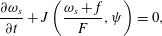 $$\begin{eqnarray}\frac{\unicode[STIX]{x2202}\unicode[STIX]{x1D714}_{s}}{\unicode[STIX]{x2202}t}+J\left(\frac{\unicode[STIX]{x1D714}_{s}+f}{F},\unicode[STIX]{x1D713}\right)=0,\end{eqnarray}$$
where
 $J$
is the Jacobian operator. The surface relative vorticity
 $\unicode[STIX]{x1D714}_{s}=v_{sx}-u_{sy}$
in terms of the transport function is
 $$\begin{eqnarray}\unicode[STIX]{x1D714}_{s}=-\frac{1}{F}\unicode[STIX]{x1D6FB}^{2}\unicode[STIX]{x1D713}+\frac{1}{F^{2}}\unicode[STIX]{x1D735}F\boldsymbol{\cdot }\unicode[STIX]{x1D735}\unicode[STIX]{x1D713}.\end{eqnarray}$$
The relevance of system (2.19)–(2.20) is that it has the same form as for a homogeneous fluid with vertically uniform vorticity
 $\unicode[STIX]{x1D714}_{s}$
and depth
 $F$
. In other words, the surface vorticity is the same for two different systems: a
 $z$
-dependent barotropic flow with vorticity
 $P(z)\unicode[STIX]{x1D714}_{s}(x,y,t)$
and depth
 $h(x,y)$
, and a homogeneous flow with vorticity
 $\unicode[STIX]{x1D714}_{s}(x,y,t)$
and depth
 $F(x,y)$
. Thus, by solving the homogeneous model one solves the vertically dependent flow. Hence the name of equivalent barotropic (Charney Reference Charney1949).
In a rapidly rotating system, the dominant terms in the vorticity equation are the linear contributions as the flow moves approximately in geostrophic balance. Geostrophy implies that
 $$\begin{eqnarray}J\left(\frac{f}{F},\unicode[STIX]{x1D713}\right)=0,\end{eqnarray}$$
which states that the flow is restricted to follow the so-called geostrophic contours
 $f/F$
because
 $\boldsymbol{v}_{s}\boldsymbol{\cdot }\unicode[STIX]{x1D735}(f/F)=0$
. For a homogeneous flow on an
 $f$
-plane (
 $\unicode[STIX]{x1D6FD}=0$
,
 $h=h(x,y)$
) the geostrophic contours are the isolines of topography (Bretherton & Haidvogel Reference Bretherton and Haidvogel1976; Zavala Sansón, González-Villanueva & Flores Reference Zavala Sansón, González-Villanueva and Flores2010). For a flat bottom on a
 $\unicode[STIX]{x1D6FD}$
-plane (
 $\unicode[STIX]{x1D6FD}\neq 0$
,
 $h=H$
constant) such contours are lines of constant latitude.
2.5 Adding forcing and dissipation
To include an external forcing and dissipative effects we introduce suitable parametrisations for the upper stress due to the wind and for the lower stress due to bottom friction. Consider the vorticity equation (2.13) but now including Laplacian viscosity and the curl of the applied stress
 $\unicode[STIX]{x1D749}(x,y,z)$
 $$\begin{eqnarray}\frac{\unicode[STIX]{x2202}\unicode[STIX]{x1D714}}{\unicode[STIX]{x2202}t}+\boldsymbol{u}\boldsymbol{\cdot }\unicode[STIX]{x1D735}\unicode[STIX]{x1D714}+\unicode[STIX]{x1D735}\boldsymbol{\cdot }\boldsymbol{u}(\unicode[STIX]{x1D714}+f)+\unicode[STIX]{x1D6FD}v+w\frac{\unicode[STIX]{x2202}\unicode[STIX]{x1D714}}{\unicode[STIX]{x2202}z}=\unicode[STIX]{x1D708}\unicode[STIX]{x1D6FB}^{2}\unicode[STIX]{x1D714}+\frac{1}{\unicode[STIX]{x1D70C}_{0}}\unicode[STIX]{x1D735}\times \frac{\unicode[STIX]{x2202}\unicode[STIX]{x1D749}}{\unicode[STIX]{x2202}z},\end{eqnarray}$$
where
 $\unicode[STIX]{x1D708}$
is the kinematic viscosity and
 $\unicode[STIX]{x1D70C}_{0}$
a reference density. The stress may be divided into two parts,
 $\unicode[STIX]{x1D749}=\unicode[STIX]{x1D749}_{a}-\unicode[STIX]{x1D749}_{b}$
, where
 $\unicode[STIX]{x1D749}_{a}$
corresponds to the wind stress at the surface and
 $\unicode[STIX]{x1D749}_{b}$
to the lower stress due to the solid bottom.
The effects of the wind stress decay at higher depths, so they are assumed to have the same vertical structure as the flow,
 $\unicode[STIX]{x1D749}_{a}=P(z)\unicode[STIX]{x1D749}_{s}(x,y)$
. The wind stress is approximated as
 $$\begin{eqnarray}\frac{1}{\unicode[STIX]{x1D70C}_{0}}\unicode[STIX]{x1D735}\times \frac{\unicode[STIX]{x2202}\unicode[STIX]{x1D749}_{a}}{\unicode[STIX]{x2202}z}\longrightarrow \frac{1}{\unicode[STIX]{x1D70C}_{0}}\unicode[STIX]{x1D735}\times \frac{\unicode[STIX]{x1D749}_{a}}{F}=\frac{P}{\unicode[STIX]{x1D70C}_{0}}\unicode[STIX]{x1D735}\times \frac{\unicode[STIX]{x1D749}_{s}}{F},\end{eqnarray}$$
which states that the wind curl only affects the upper layer of depth
 $F$
. This parametrisation is equivalent to that used in earlier studies (Krupitsky et al.
Reference Krupitsky, Kamenkovich, Naik and Cane1996; LaCasce & Isachsen Reference LaCasce and Isachsen2010).
At the lower boundary we assume that the stress is proportional to the bottom relative vorticity,
 $\unicode[STIX]{x1D749}_{b}=R\unicode[STIX]{x1D714}_{b}$
, where
 $R$
is a constant with units of (m
 $\text{s}^{-1}$
). Thus, the bottom friction term is
 $$\begin{eqnarray}\frac{1}{\unicode[STIX]{x1D70C}_{0}}\unicode[STIX]{x1D735}\times \frac{\unicode[STIX]{x2202}\unicode[STIX]{x1D749}_{b}}{\unicode[STIX]{x2202}z}\longrightarrow \frac{R}{h}\unicode[STIX]{x1D714}_{b}=\frac{R}{h}P(-h)\unicode[STIX]{x1D714}_{s},\end{eqnarray}$$
where the exponential structure function over the topography is
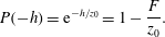 $$\begin{eqnarray}P(-h)=\text{e}^{-h/z_{0}}=1-\frac{F}{z_{0}}.\end{eqnarray}$$
Parametrisations (2.23) and (2.24) are inserted in the vorticity equation (2.22). Then we proceed as before, integrating from
 $-h$
to 0, dividing over
 $F$
and omitting the
 $(1-G/F)$
term,
 $$\begin{eqnarray}\frac{\unicode[STIX]{x2202}\unicode[STIX]{x1D714}_{s}}{\unicode[STIX]{x2202}t}+J\left(\frac{\unicode[STIX]{x1D714}_{s}+f}{F},\unicode[STIX]{x1D713}\right)=\unicode[STIX]{x1D708}\unicode[STIX]{x1D6FB}^{2}\unicode[STIX]{x1D714}_{s}+\frac{1}{\unicode[STIX]{x1D70C}_{0}}\unicode[STIX]{x1D735}\times \frac{\unicode[STIX]{x1D749}_{s}}{F}-R\left(\frac{1}{F}-\frac{1}{z_{0}}\right)\unicode[STIX]{x1D714}_{s}.\end{eqnarray}$$
This is the vorticity equation of the equivalent-barotropic dynamics with exponential
 $P(z)$
, and including forcing and dissipation. The most relevant aspect of the bottom friction term is the dependence on
 $F$
and the parameter
 $z_{0}$
. When
 $z_{0}\gg h$
then
 $F=h$
and the linear Ekman friction of the homogeneous model is recovered,
 $-R\unicode[STIX]{x1D714}_{s}/h$
(Zavala Sansón & van Heijst Reference Zavala Sansón and van Heijst2002). More importantly, for shallow
 $F$
the factor
 $(1/F-1/z_{0})$
is reduced as
 $z_{0}$
decreases (the limit value is 0 as
 $z_{0}\rightarrow F$
, so the factor never becomes negative). As a consequence, bottom friction becomes less important when flow motions predominate near the surface. In other words, the model captures the reduction of frictional effects due to the lower boundary when the vertical structure decays rapidly (in such cases, of course, one must keep in mind that the nonlinear model might contain a greater error).
2.6 Numerical scheme
The governing equations are solved in a rectangular grid with a finite differences code, originally developed by Orlandi and Verzicco for two-dimensional flows (see e.g. Orlandi & van Heijst (Reference Orlandi and van Heijst1992)). The nonlinear terms are spatially discretised with an Arakawa scheme (which avoids the spurious production of energy/enstrophy in the inviscid limit), and in time with an explicit, third-order Runge–Kutta method. The viscous terms are treated implicitly with a centred, second-order scheme. van Geffen included rotational effects and several additional features (van Geffen & Davies Reference van Geffen and Davies2000). The code was modified independently by the author to include variable topography effects by solving the vorticity-transport function equation with a multigrid method (for a purely 2-D flow, such expression is reduced to the Poisson equation, which is solved with a fast Fourier transform in the original scheme). By also adding viscous topographic effects (i.e. Ekman friction), the code has been applied in numerous studies to simulate the evolution of quasi-2-D vortices and currents in laboratory experiments (see Zavala Sansón & van Heijst (Reference Zavala Sansón, van Heijst, von Larcher and Williams2014) and references therein). Recently, an external forcing term was included to simulate experimental observations of continuously forced shear flows (González Vera & Zavala Sansón Reference González Vera and Zavala Sansón2015). Summarising, the code solves the motion of a homogeneous flow with vertically uniform vorticity
 $\unicode[STIX]{x1D714}$
and fluid depth
 $h$
. The equivalent-barotropic equations, equations (2.20) and (2.26), are solved with the same formulation using the uniform vorticity
 $\unicode[STIX]{x1D714}_{s}$
and the equivalent depth
 $F$
. In all examples shown below, there are
 $257\times 257$
grid points. The time step
 $\text{d}t$
is chosen to satisfy a Courant number criterion (
 $Cr<\sqrt{3}$
) to ensure numerical stability in each specific problem.
3 Vortices around seamounts
In this section, numerical simulations of strong cyclonic vortices in the presence of a submarine mountain are presented. This problem was selected to illustrate the modification of nonlinear effects in barotropic flows with a vertical structure, so the
 $\unicode[STIX]{x1D6FD}$
- and wind-forcing terms are omitted. Laboratory experiments and numerical simulations of a purely barotropic vortex in the vicinity of a seamount were performed by Zavala Sansón et al. (Reference Zavala Sansón, Barbosa Aguiar and van Heijst2012), so that study serves as a reference to compare with the present simulations. The essential feature of the problem is that a nonlinear vortex drifts around the mountain in clockwise direction, i.e. with shallow water to the right. Also, there is the formation of negative relative vorticity on the mountain summit due to squeezing effects of fluid columns. The aim here is to illustrate how the vortex drift is modified according to the vertical structure of the flow when using the equivalent-barotropic dynamics. Before presenting the results, we describe first the numerical flow parameters. Afterwards, we present the vortex behaviour in simulations with different
 $z_{0}$
-values and illustrations of the vertical velocity field.
3.1 Flow parameters
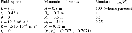
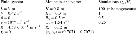
Table 1 shows the parameters of the fluid system, the topographic mountain and the initial, cyclonic vortex. Most of the parameters are taken from the barotropic simulation shown in figures 12 and 13 of Zavala Sansón et al. (Reference Zavala Sansón, Barbosa Aguiar and van Heijst2012), which simulates the experimental observations effectively. The numerical domain is a square with half-length
 $L$
 $\{x,y|-L\leqslant x\leqslant L,-L\leqslant y\leqslant L\}$
and no-slip boundary conditions. We consider the
 $f$
-plane approximation, so
 $\unicode[STIX]{x1D6FD}=0$
and
 $f=f_{0}$
(with the rotation period
 $T=4\unicode[STIX]{x03C0}/f_{0}$
).
Flow parameters in the simulations of cyclonic vortices in the presence of a submarine mountain. The spatial resolution is
 $257\times 257$
grid points and the numerical time step
 $\text{d}t=0.3$
s. The rotation period is
 $T=4\unicode[STIX]{x03C0}/f_{0}=30$
s.
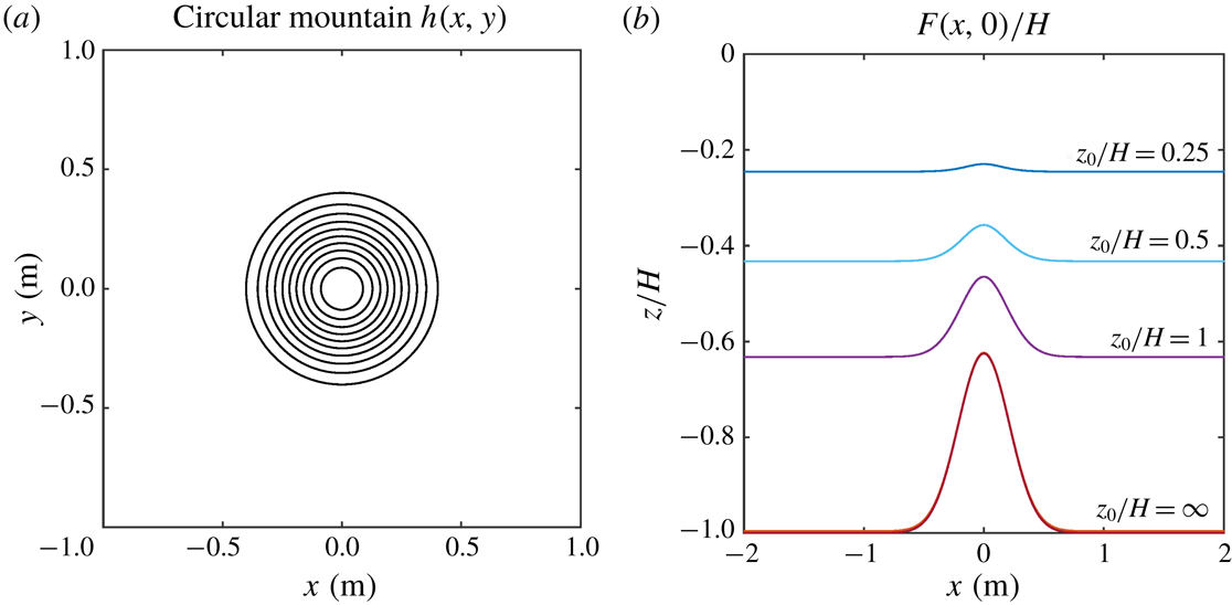
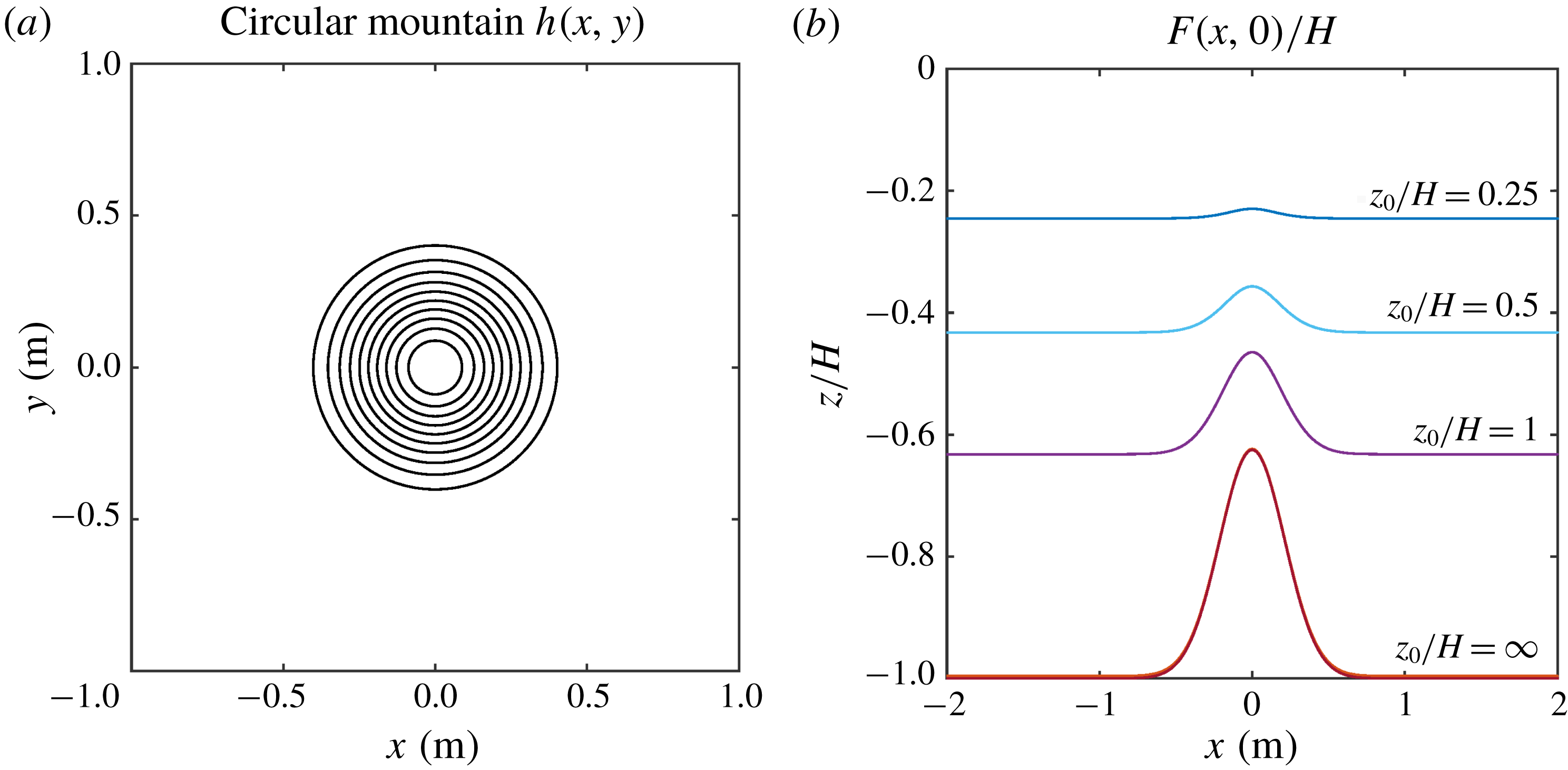
(a) Depth contours of the submarine mountain (3.1). Outer (inner) contour is
 $0.75$
m (
 $0.525$
m); the contour interval is 0.025 m. (b) Normalised equivalent depth profiles
 $F(x,0)/H$
calculated with the
 $e$
-folding depths
 $z_{0}/H=\infty$
, 1, 0.5 and 0.25. Case
 $z_{0}/H=\infty$
corresponds to the homogeneous flow with
 $F(x,y)=h(x,y)$
.
The topographic mountain has an exponential shape centred at the origin, such that the fluid depth is
 $$\begin{eqnarray}h(x,y)=H-H_{m}\exp \left[-\frac{(x^{2}+y^{2})}{0.36R_{m}^{2}}\right],\end{eqnarray}$$
where
 $H$
is the maximum depth (away from the mountain),
 $H_{m}$
the height of the topography and
 $R_{m}$
its radial scale. Figure 1(a) shows the circular topography contours. In the absence of
 $\unicode[STIX]{x1D6FD}$
, the
 $h$
-contours have the same shape as the geostrophic contours,
 $f_{0}/h$
. The equivalent depth
 $F$
is calculated with (2.3). Four equivalent-barotropic simulations with different non-dimensional
 $e$
-folding depths
 $z_{0}/H$
are performed:
 $z_{0}/H\gg 1$
(corresponding to the homogeneous case), 1, 0.5 and 0.25. Figure 1(b) presents the corresponding
 $F(x,0)$
profiles across the mountain. Note that the equivalent depth field gives a smoothed mountain in a shallower fluid layer as
 $z_{0}$
is reduced.
Bottom friction is determined by the Ekman pumping/blowing condition at the lower boundary layer with thickness
 $\unicode[STIX]{x1D6FF}_{E}=(2\unicode[STIX]{x1D708}/f_{0})^{1/2}\approx 0.0022$
mm. For a homogeneous model, the main contribution of Ekman friction is a linear term
 $-\unicode[STIX]{x1D6FF}_{E}\,f_{0}\unicode[STIX]{x1D714}/(2h)\equiv -R\unicode[STIX]{x1D714}/h$
(Zavala Sansón & van Heijst Reference Zavala Sansón and van Heijst2002), so the friction coefficient is
 $R=\unicode[STIX]{x1D6FF}_{E}\,f_{0}/2$
.
The initial condition is a well-known cyclonic vortex with azimuthal velocity profile (van Heijst & Clercx Reference van Heijst and Clercx2009)
 $$\begin{eqnarray}V(r)=\frac{\unicode[STIX]{x1D714}_{v}R_{v}^{2}}{2r}\left[1-\exp (-r^{2}/R_{v}^{2})\right],\end{eqnarray}$$
where
 $r^{2}=(x-x_{c})^{2}+(y-y_{c})^{2}$
with
 $(x_{c},y_{c})$
the vortex initial position;
 $\unicode[STIX]{x1D714}_{v}$
is the initial peak vorticity and
 $R_{v}$
its radial scale. The velocity decays as
 $1/r$
at long distances. The initial Rossby number is
 $V(R_{v})/(f_{0}R_{v})=1.1$
, but after one rotation period, the structure is adjusted in a more geostrophic regime. The vortex initial position is close enough to the mountain so the topographic effects are important, and far enough from the lateral walls so the influence of the walls is negligible.
3.2 Vortex evolution
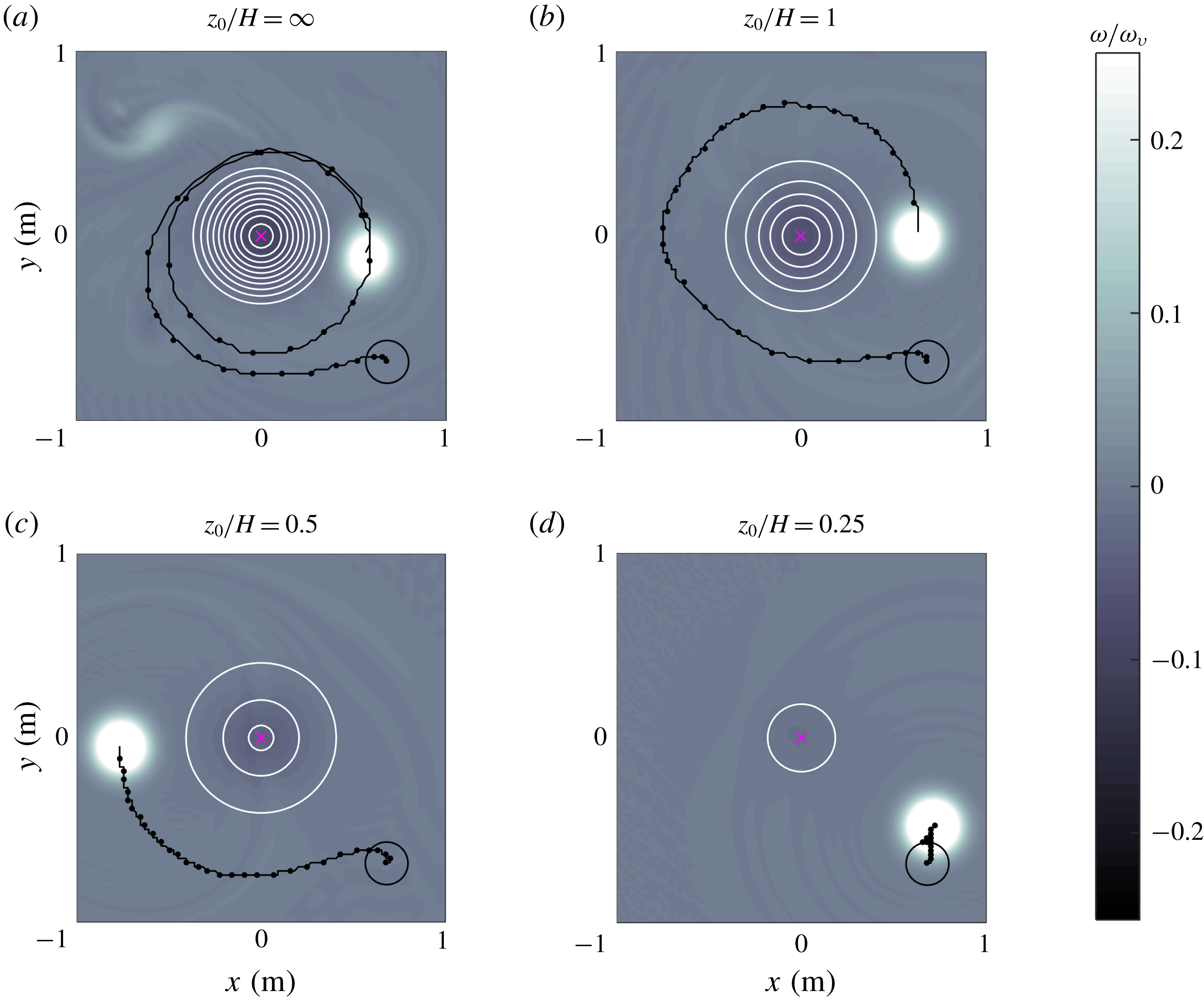
Relative vorticity fields numerically calculated at
 $t/T=31.5$
in four simulations of vortices around a seamount: (a)
 $z_{0}/H=\infty$
(homogeneous flow), (b)
 $z_{0}/H=1$
, (c)
 $z_{0}/H=0.5$
, (d)
 $z_{0}/H=0.25$
. The vortex parameters and initial positions (indicated with a black circle) are the same in all cases (see table 1). Vorticity values are normalised with the initial peak vorticity
 $\unicode[STIX]{x1D714}_{v}$
. The trajectory of the maximum vorticity at the vortex centre is shown every
 $0.15~T$
. White circles are
 $F$
-contours with outer (inner) values of: (a) 0.74 m (0.515 m), (b) 0.49 m (0.39 m), (c) 0.29 m (0.34 m), (d) 0.19 m. In all cases the contour interval is 0.025 m.
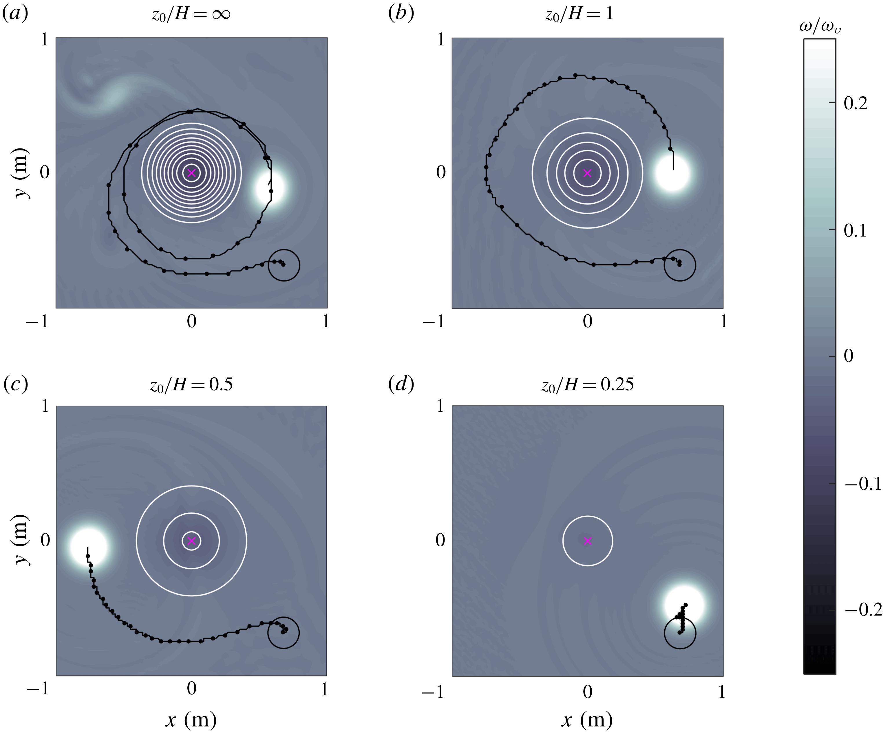
The behaviour of a homogeneous vortex (
 $z_{0}/H\gg 1$
) is examined first. Figure 2(a) shows the relative vorticity field and vortex trajectory at time
 $t/T=31.5$
. The vortex drifts almost two turns around the mountain, and there is the formation of negative vorticity on top of the topography (a secondary result is the formation of a weaker cyclonic patch at the upper-left part of the panel that is generated at the beginning of the simulations when fluid over the mountain is displaced downhill, acquiring positive vorticity). This plot can be compared with the simulation presented in figure 13(a) of Zavala Sansón et al. (Reference Zavala Sansón, Barbosa Aguiar and van Heijst2012). The results are not exactly the same because the parametrisation of bottom friction effects is slightly different (in that study, weakly nonlinear Ekman effects were included).
Figure 2(b) shows the equivalent-barotropic case with
 $z_{0}/H=1$
. The vortex behaviour can be explained by considering the shape of the equivalent depth
 $F$
, as shown in figure 1
b). The influence of the smoothed topography implies that now the vortex drift around the mountain is slower in comparison with the homogeneous case: the vortex completes less than one turn after the same time lapse. For smaller
 $z_{0}$
the vortex drift is progressively shorter, as shown in figure 2(c,d) for
 $z_{0}/H=0.5$
and 0.25, respectively. In the latter case, the vortex experiences a very weak influence of the almost-flat topography
 $F$
. These results may be thought in terms of the barotropic flow with vertical structure
 $\text{e}^{z/z_{0}}$
and depth
 $h$
. The decay rate of the surface variables
 $(1/z_{0})$
reduces the effects of the bottom topography for smaller
 $z_{0}$
. In the last example (
 $z_{0}/H=0.25$
), the topography is nearly flat (see figure 1
b), so the vortex is barely influenced by the mountain and therefore is only displaced a short distance from the original location.
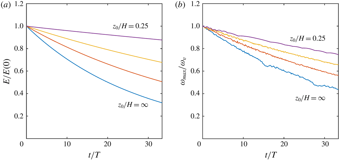
Time evolution of normalised (a) total energy and (b) peak vorticity calculated in the simulations shown in figure 2:
 $z_{0}/H=\infty$
(lower curves), 1, 0.5 and 0.25.
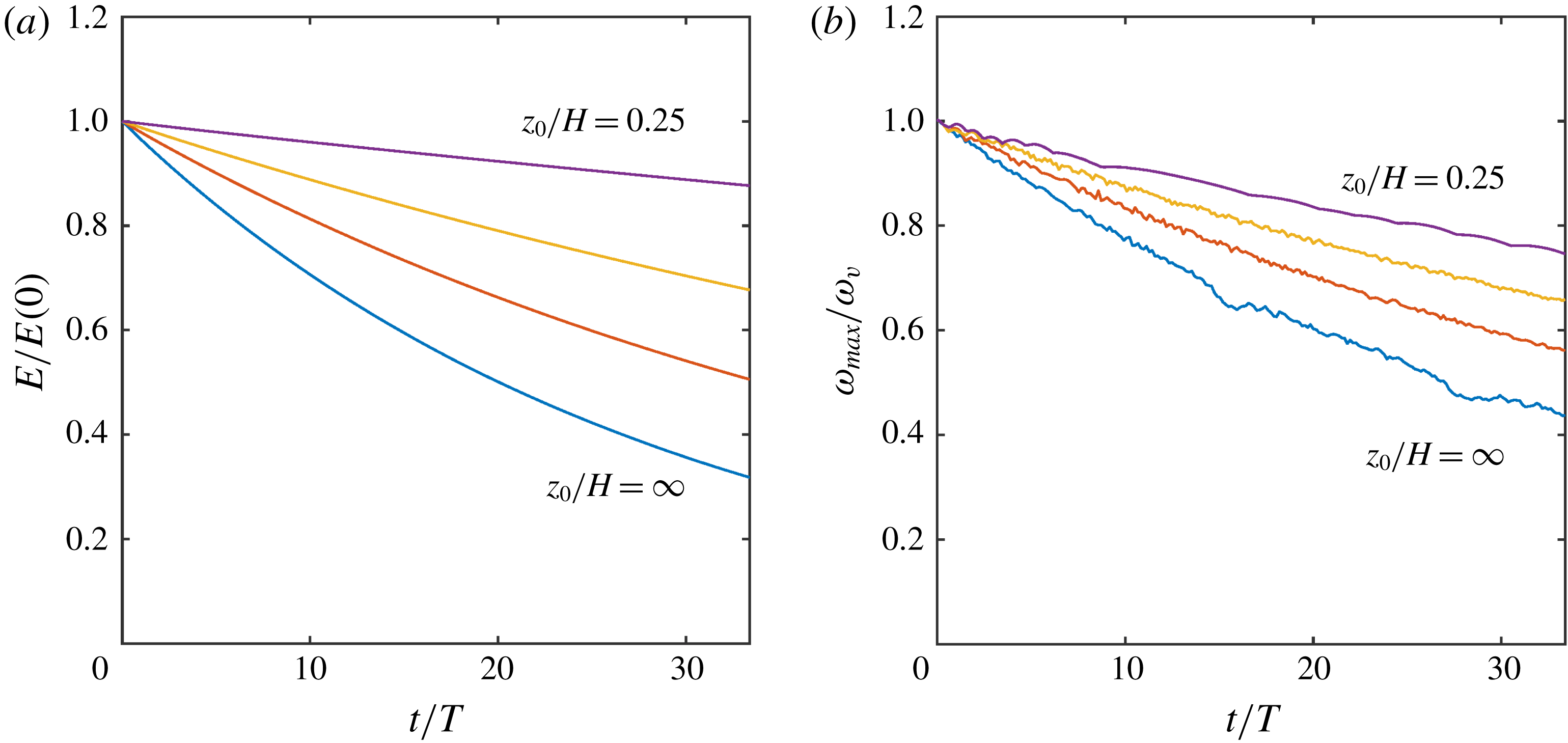
To appreciate the effects of bottom friction in the simulations, we calculate the time evolution of the total kinetic energy
 $E$
over the whole volume and the peak vorticity at the vortex centre. In the
 $(\unicode[STIX]{x1D714}_{s},F)$
equivalent-barotropic system, the energy (per mass unit) is
 $E=(1/2)\int _{A}\int _{-F}^{0}(u_{s}^{2}+v_{s}^{2})\,\text{d}z\,\text{d}A$
where
 $\text{d}A$
is the differential horizontal area. The quadratic term
 $w^{2}$
is considered negligible because it is proportional to
 $(1-P)^{2}$
. It is easy to show that
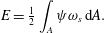 $$\begin{eqnarray}E={\textstyle \frac{1}{2}}\int _{A}\unicode[STIX]{x1D713}\unicode[STIX]{x1D714}_{s}\,\text{d}A.\end{eqnarray}$$
If the energy is calculated in the
 $(P\unicode[STIX]{x1D714}_{s},h)$
system the result is the same, with an error
 $(1-G/F)$
multiplied by quadratic terms. Figure 3 presents the time evolution of the normalised kinetic energy and maximum vorticity in the four simulations. In both plots, the decay is stronger in the purely barotropic case (
 $z_{0}/H\gg 1$
), and such a behaviour is progressively weaker for smaller
 $z_{0}$
. The reason is that bottom friction effects are proportional to
 $(1/F-1/z_{0})$
, so they are reduced for flows with a vertical structure. The flow experiences not only a weaker topographic slope but also a decreased bottom friction.
3.3 Vertical velocity
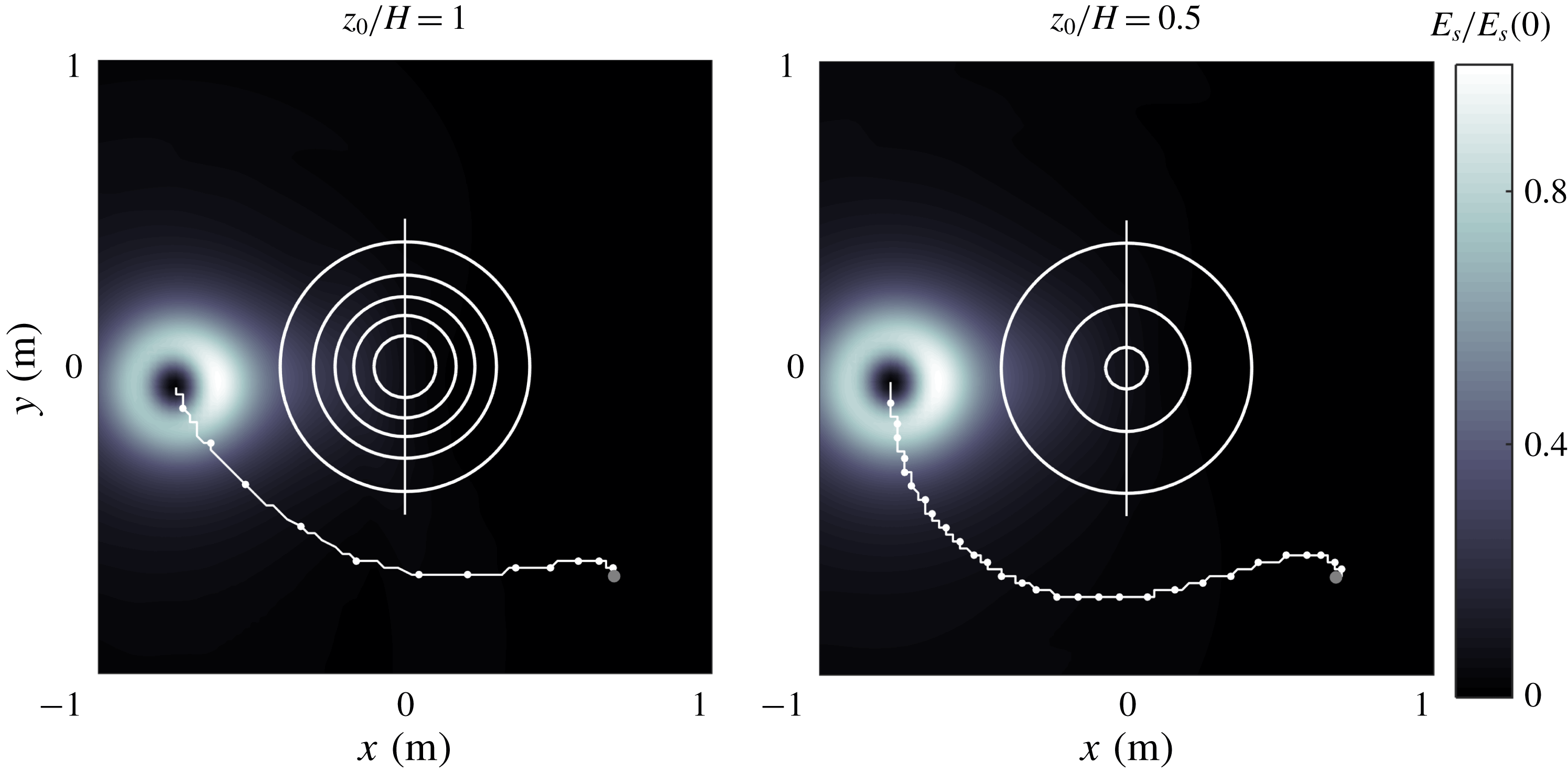
Surface kinetic energy field in two simulations with cyclonic vortices passing at the left flank of the mountain: (a)
 $z_{0}/H=1$
,
 $t/T=13.5$
. (b)
 $z_{0}/H=0.5$
,
 $t/T=31.6$
. The trajectory of the maximum vorticity at the vortex centre is shown every
 $0.15T$
. White circles are
 $F$
-contours as in figure 2(b,c). The straight line across the mountain indicates the position of the vertical planes used in figure 5.
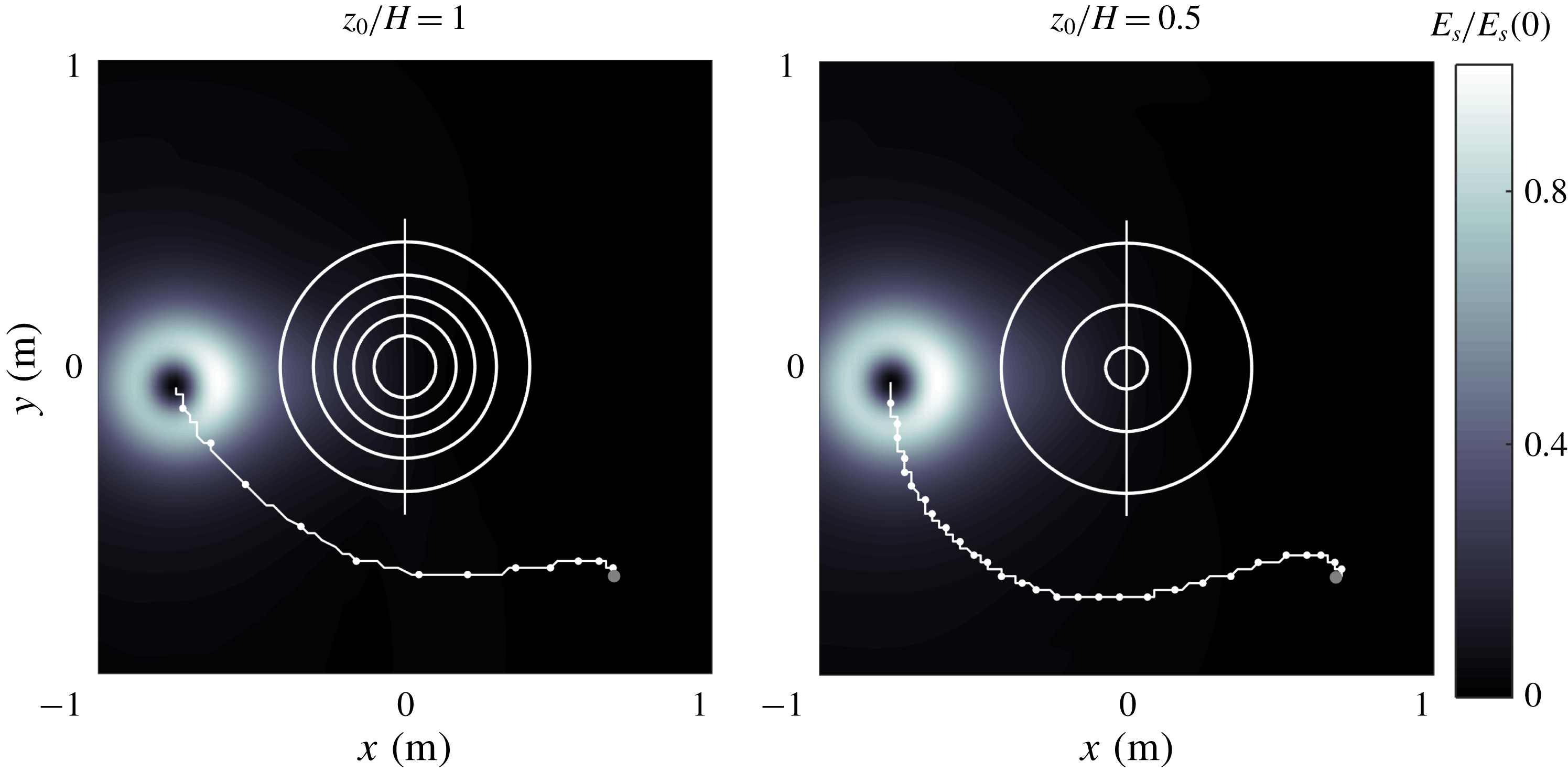
Given the horizontal surface solutions
 $(u_{s},v_{s},0)$
it is possible to reconstruct the 3-D velocity field
 $(Pu_{s},Pv_{s},w)$
and investigate the vertical characteristics of the equivalent-barotropic flows. We consider the simulations with
 $z_{0}/H=1$
and 0.5. To make a fair comparison, it is necessary to select specific times at which the vortices in these cases are in a similar position during their translation around the mountain. Figure 4 presents the surface kinetic energy field
 $E_{s}=(u_{s}^{2}+v_{s}^{2})/2$
at a time when the corresponding vortices are located at the left flank of the mountain. Note the kinetic energy intensification at the side facing the topography. The vortex with
 $z/H=1$
(panel a) drifts at a faster speed and reaches that point at an earlier time than the vortex with
 $z/H=0.5$
(panel b). In these positions, the vortices generate an intense flow in the positive
 $y$
-direction over the mountain. The aim is to compare the vertical velocity fields on the vertical plane at
 $x=0$
, indicated with a straight line in both panels.
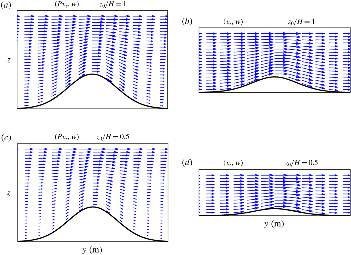
Velocity fields on a vertical plane
 $x=0$
over the mountain (see figure 4). (a,b)
 $z_{0}/H=1$
, with maximum speed
 $0.054~\text{m}~\text{s}^{-1}$
. (c,d)
 $z_{0}/H=0.5$
, with maximum speed
 $0.048~\text{m}~\text{s}^{-1}$
. In (a,c) the vertical velocity is calculated with (2.9), the depth profile is
 $h(x,y)$
and the vertical axis
 $-H\leqslant z\leqslant 0$
. In (b,d) the vertical velocity is given by (2.7), the depth profile is
 $F(x,y)$
and the vertical axis
 $-F_{max}\leqslant z\leqslant 0$
, where
 $F_{max}$
is the maximum value of the equivalent depth.
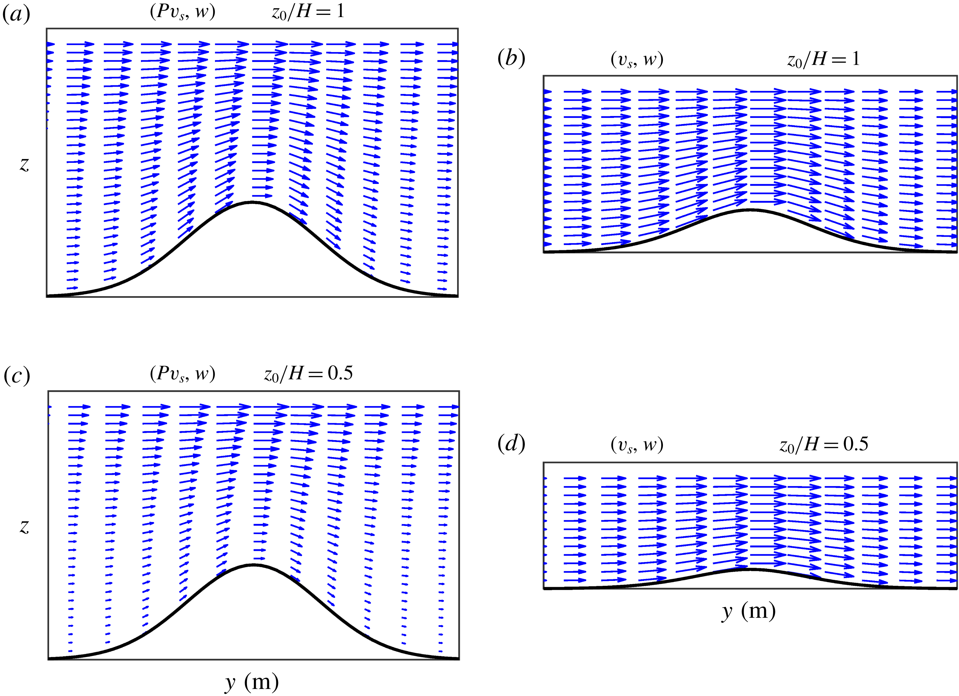
Figure 5 shows the vertical velocity fields calculated in the two simulations. Consider first the case with
 $z/H=1$
. In terms of the barotropic flow with vertical structure
 $P(z)$
and depth
 $h$
, the velocity field is
 $(Pv_{s},w)$
, shown in figure 5(a). The flow is intensified as fluid columns are squeezed over the mountain summit. Note the flow decay with depth due to
 $P(z)$
. The vertical velocity
 $w$
is given by (2.9). It is verified that this component is zero at the surface,
 $w(0)=0$
, and the flow is tangent to the bottom topography, according to the boundary condition
 $w(-h)=-P(-h)v_{s}h_{y}$
(with
 $u_{s}\sim 0$
at this time). When the problem is thought of as a purely barotropic flow over the smoothed topography
 $F$
, the velocity field is
 $(v_{s},w)$
, shown in figure 5(b). Now the horizontal component is uniform over the (equivalent) fluid depth, and the vertical velocity is calculated with (2.7). Recall that both fields have the same surface velocity component
 $v_{s}$
. Thus, the effect of the vertical decay in panel a is mimicked with the smoothed topography in panel (b). Analogous plots of the vertical velocity fields for the simulation with
 $z/H=0.5$
are shown in figure 5(c,d). The equivalent fluid system with a depth of
 $F$
becomes very shallow (panel d).
The vertical structure in the two simulations can be compared with figure 5(a,c). It is noted that the velocity field decays with depth at a faster rate for smaller
 $z_{0}$
(panel c). As a result, the topographic effects of the mountain slopes are reduced, and the vortex drifts at a slower speed.
4 Wind-driven flow
In this section, the planetary
 $\unicode[STIX]{x1D6FD}$
-effect and wind forcing are addressed. We examine the evolution of a large-scale, wind-driven oceanic flow in a closed basin with topography, in which nonlinear effects are secondary. The classical Stommel problem consists of a single homogeneous fluid layer, subject to a uniform wind stress acting along the zonal direction in a flat-bottomed, square basin (Stommel Reference Stommel1948). For steady, linear flow and anticyclonic forcing, the vorticity equation has exact analytical solutions in which the wind-stress curl, bottom friction and
 $\unicode[STIX]{x1D6FD}$
-effect are balanced. The solutions consist of a large-scale, anticyclonic gyre covering the whole domain, intensified at the western boundary (in the Northern Hemisphere).
Numerical simulations of the Stommel problem are performed, but now including (i) topographic effects due to the continental slopes near the walls of the basin, and (ii) the vertical structure of the flow according to the equivalent-barotropic formulation. Salmon (Reference Salmon1998) discussed the Stommel problem with topography for a double-gyre structure in a rectangular domain. The aim of the present simulations is to show the modification of single oceanic gyres due to the new dynamical conditions. We discuss first the flow parameters, the forcing and the topographic basin. Afterwards, we present the results for the homogeneous case, followed by the results for equivalent-barotropic flows.
4.1 Flow parameters
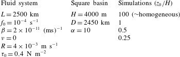
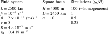
Table 2 shows the flow parameters of the system and the topographic basin. The numerical domain is again a square with half-length
 $L$
, centred at the origin of a Cartesian
 $x,y$
-coordinate system, with the coordinate
 $x$
(
 $y$
) along the zonal (latitudinal) direction. The rotation parameters
 $f_{0}$
and
 $\unicode[STIX]{x1D6FD}$
are typical of a mid-latitude ocean. Laplacian viscosity is omitted, and free-slip boundary conditions are considered.
Flow parameters in the simulations of the Stommel problem with topography. The spatial resolution is
 $257\times 257$
grid points and the time step
 $\text{d}t=3600$
s.
The topography is a square basin of the form
 $$\begin{eqnarray}h(x,y)=H\exp \left(-\frac{|x|^{\unicode[STIX]{x1D6FC}}+|y|^{\unicode[STIX]{x1D6FC}}}{D^{\unicode[STIX]{x1D6FC}}}\right),\end{eqnarray}$$
with maximum depth
 $H$
at the domain centre and slopes near the walls. The steepness of the slopes depends on the scale
 $D$
and the exponent
 $\unicode[STIX]{x1D6FC}$
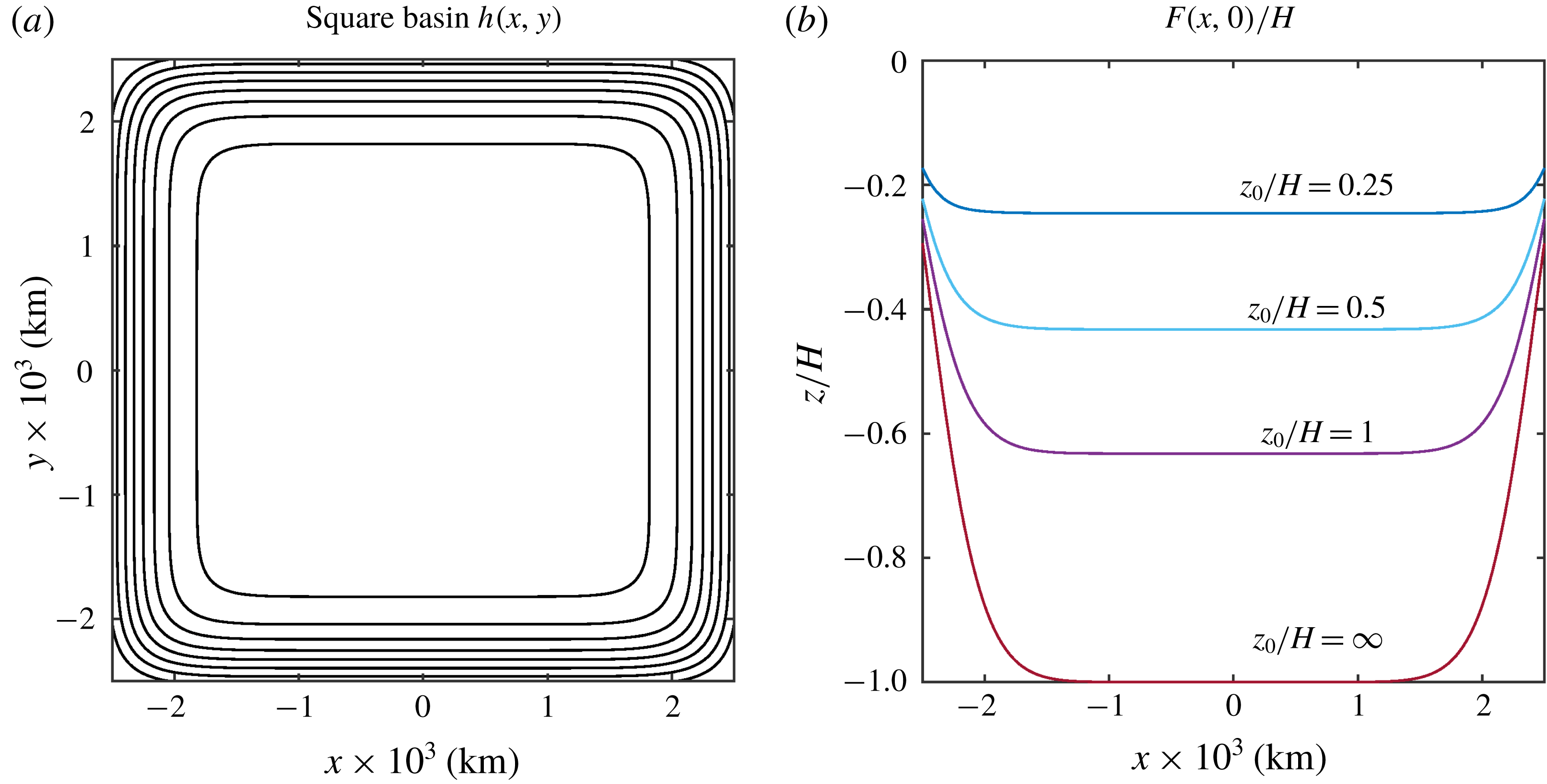
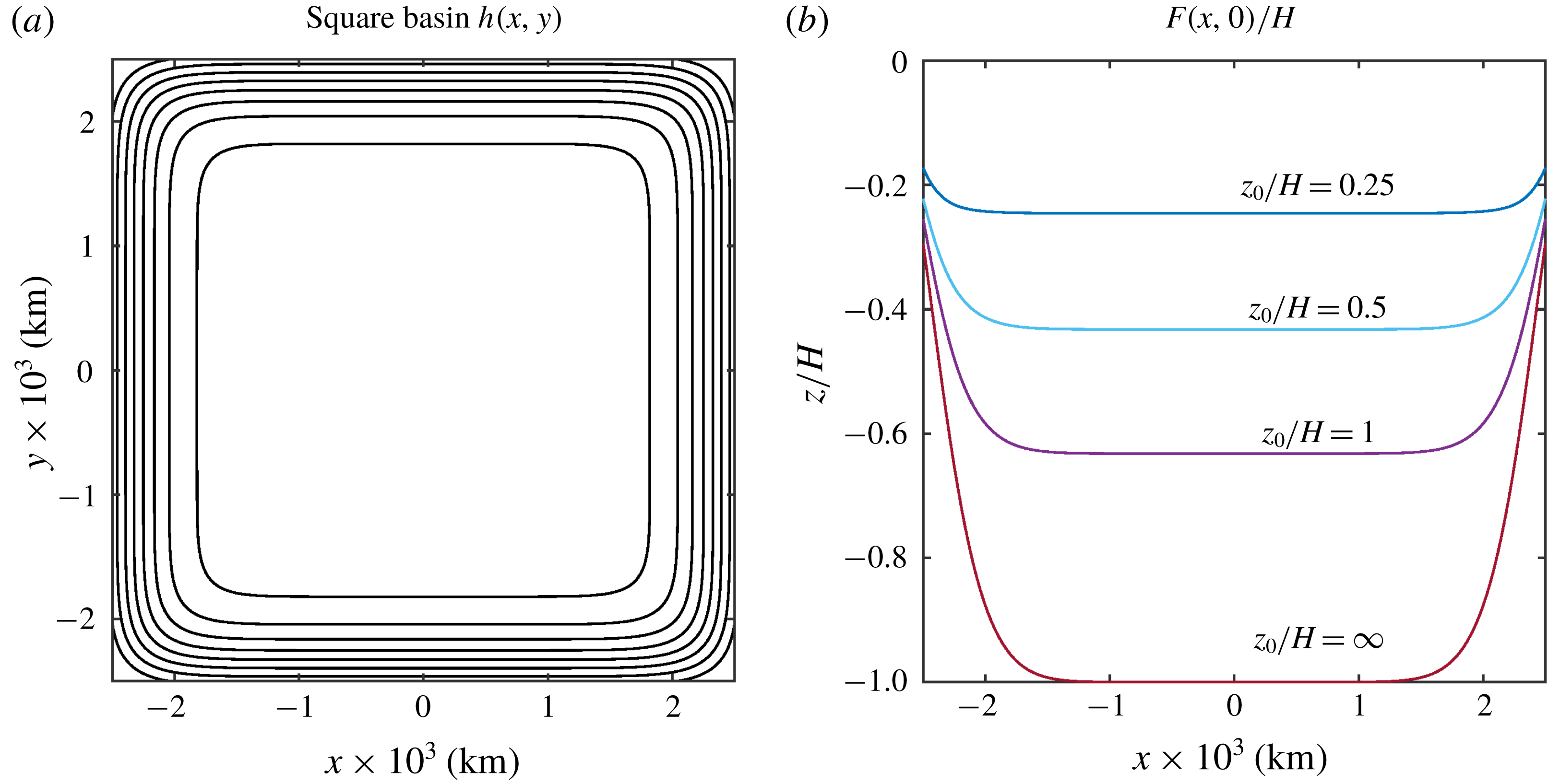
. For the chosen parameters the topography is nearly flat at the central part of the domain and has abrupt slopes along the walls, as shown in figure 6(a). Four simulations with different
 $z_{0}/H$
are presented:
 $z_{0}/H=100$
, 1, 0.5 and 0.25. The corresponding zonal profiles of the equivalent depth,
 $F(x,0)$
, are shown in figure 6(b). The deepest curve corresponds to the homogeneous system with
 $F=h$
. In the other cases, the equivalent depth is a shallower basin with less steep slopes (as we saw for the topographic mountain).
(a) Depth contours of the oceanic square basin (4.1). Outer (inner) contour is
 $1000$
m (
 $3800$
m); the contour interval is 400 m. (b) Normalised equivalent depth profiles
 $F(x,0)/H$
calculated with the
 $e$
-folding depth
 $z_{0}/H=\infty$
, 1, 0.5 and 0.25.
The single-gyre solution of the Stommel problem is obtained with a uniform stress acting along the zonal direction
 $$\begin{eqnarray}\unicode[STIX]{x1D749}_{s}=(\unicode[STIX]{x1D70F}^{x},\unicode[STIX]{x1D70F}^{y})=\left(-\unicode[STIX]{x1D70F}_{0}\cos \left[\frac{\unicode[STIX]{x03C0}}{2L}(y+L)\right],0\right),\end{eqnarray}$$
where
 $\unicode[STIX]{x1D70F}_{0}$
is the stress amplitude. In the numerical code, the curl of the wind stress in the vorticity equation is written as
 $$\begin{eqnarray}\frac{1}{\unicode[STIX]{x1D70C}_{0}}\unicode[STIX]{x1D735}\times \frac{\unicode[STIX]{x1D749}_{s}}{F}=\frac{1}{\unicode[STIX]{x1D70C}_{0}}\left(\frac{1}{F}\unicode[STIX]{x1D735}\times \unicode[STIX]{x1D749}_{s}+\frac{F_{y}}{F^{2}}\unicode[STIX]{x1D70F}^{x}\right)(1-\text{e}^{-t/t_{i}}).\end{eqnarray}$$
The time-dependent factor at the right-hand side is used to set the flow at rest initially and then apply the forcing gradually. As time progresses, the wind-stress curl rapidly reaches a steady state value in a time scale
 $t_{i}=12\,\text{d}t$
(half a day).
The linear friction coefficient
 $R=\unicode[STIX]{x1D6FF}_{E}\,f_{0}/2$
is estimated with a bottom Ekman layer of approximately 80 m (see previous section). With the chosen combination of forcing and friction coefficients
 $(\unicode[STIX]{x1D70F}_{0},R)$
, the interior flow speed in the homogeneous simulation varies between 0.01 and
 $0.03~\text{m}~\text{s}^{-1}$
, while the intensified western flow is about
 $0.3~\text{m}~\text{s}^{-1}$
. For the equivalent-barotropic simulations, the chosen
 $(\unicode[STIX]{x1D70F}_{0},R)$
-values may lead to unrealistic high speeds because the forcing (topography) effects are enhanced (inhibited), as shall be discussed below. Despite this, the simulations are useful to illustrate the effects of changing only the vertical structure of the flow. A different procedure would be to modify the
 $(\unicode[STIX]{x1D70F}_{0},R)$
pair to obtain similar root-mean-square (r.m.s.) velocities in experiments with different
 $z_{0}$
.
4.2 The Stommel problem with topography
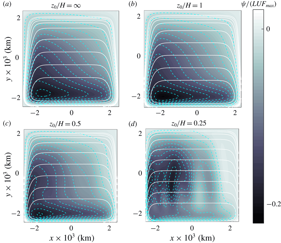
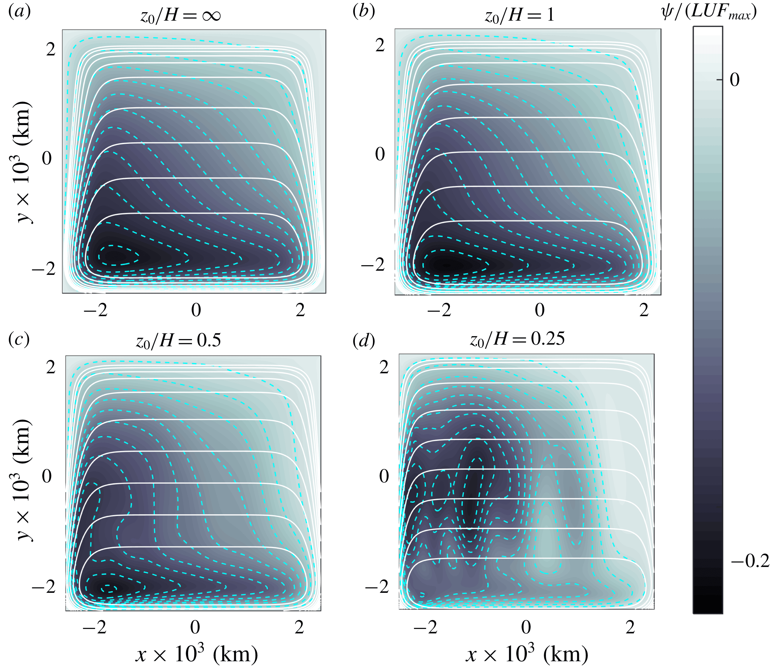
The homogeneous case is presented first. Initially, the large-scale, anticyclonic gyre that characterises the Stommel solution is formed as the forcing is applied. After approximately 30 days the flow reaches a steady state which, however, is very different to the traditional Stommel gyre. Figure 7(a) shows the transport function field at
 $t=45$
days, superposed with the geostrophic
 $f/h$
contours. Due to the
 $\unicode[STIX]{x1D6FD}$
-term, the
 $f/h$
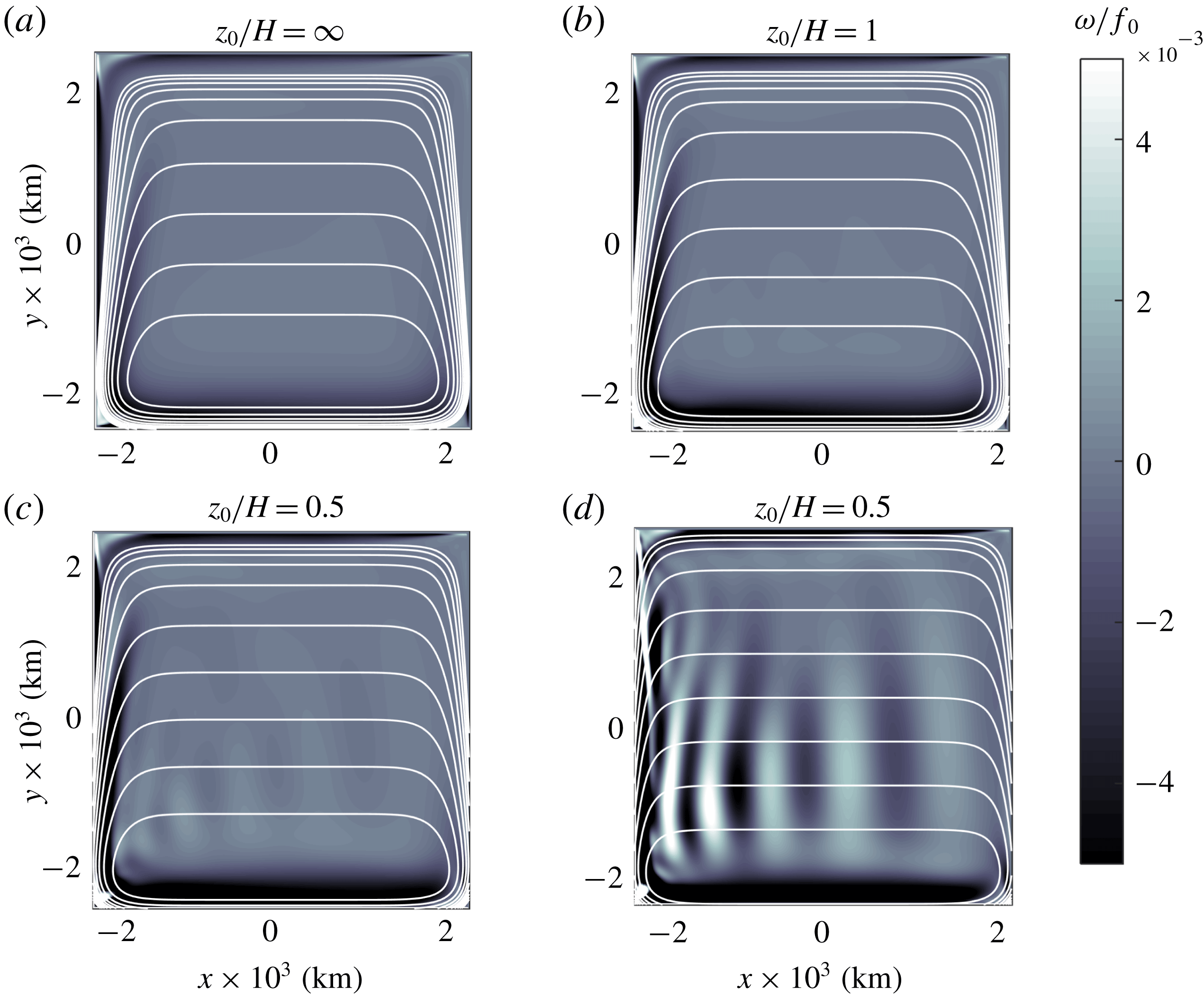
contours are trapezoidal, with the base parallel to the southern wall. The anticyclonic circulation is strongly deformed and displaced towards the south-western corner of the domain. The northward flow detaches from the western boundary and follows the geostrophic contours, indicating that the linear terms predominate. Figure 8(a) presents the relative vorticity surfaces of the resulting flow, also superposed with the planetary vorticity contours. The vorticity field shows more clearly the structure and latitudinal position of the northward flow detached from the western wall. Besides, as the large-scale gyre acquires its southern latitude, a negative vorticity strip is formed over the topographic slope, parallel to the wall.
Transport function fields numerically calculated at
 $t=45$
days in four simulations of the Stommel problem: (a)
 $z_{0}/H=\infty$
(homogeneous flow), (b)
 $z_{0}/H=1$
, (c)
 $z_{0}/H=0.5$
, (d)
 $z_{0}/H=0.25$
. The
 $\unicode[STIX]{x1D713}$
-values are normalised with
 $ULF_{max}$
, where
 $U=[0.04,0.06,0.07,0.12]~\text{m}~\text{s}^{-1}$
is the r.m.s. velocity and
 $F_{max}=[4000,2528,1729,982]$
m the maximum equivalent depth. Segmented curves indicate the normalised
 $\unicode[STIX]{x1D713}$
-contours
 $[-0.22:0.02:-0.02]$
. Solid curves are geostrophic contours
 $(f_{0}+\unicode[STIX]{x1D6FD}y)/F(x,y)$
. The minimum contours in the interior are
 $c_{min}=[0.17,0.25,0.36,0.59]\times 10^{-7}~(\text{ms})^{-1}$
, respectively, with contour interval
 $c_{min}/5$
.
The southward displacement of the large-scale circulation is due to the topographic
 $\unicode[STIX]{x1D6FD}$
-effect associated with the western bottom slope, which favours the tendency of the gyre to move towards the local ‘western’ direction, that is, to the geographical south. This result has been discussed previously by other authors in the context of large-scale, forced circulations (Salmon Reference Salmon1998) or in the context of unforced, mesoscale vortices over sloping bottom topographies (Grimshaw et al.
Reference Grimshaw, Tang and Broutman1994; Zavala Sansón & van Heijst Reference Zavala Sansón and van Heijst2000).
The flow configuration (a steady, large-scale circulation at the southern region of the domain) is very robust. The persistence of the solutions and its linear character implies that a new balance occurs in the vorticity equation. Such a balance is between the topographic,
 $\unicode[STIX]{x1D6FD}$
, forcing and bottom friction terms,
 $$\begin{eqnarray}J\left(\frac{f_{0}}{h},\unicode[STIX]{x1D713}\right)-\frac{\unicode[STIX]{x1D6FD}}{h}\frac{\unicode[STIX]{x2202}\unicode[STIX]{x1D713}}{\unicode[STIX]{x2202}x}=\frac{1}{\unicode[STIX]{x1D70C}_{0}}\unicode[STIX]{x1D735}\times \frac{\unicode[STIX]{x1D749}_{s}}{h}-\frac{R}{h}\left(-\frac{1}{h}\unicode[STIX]{x1D6FB}^{2}\unicode[STIX]{x1D713}+\frac{1}{h^{2}}\unicode[STIX]{x1D735}h\boldsymbol{\cdot }\unicode[STIX]{x1D735}\unicode[STIX]{x1D713}\right),\end{eqnarray}$$
where the wind curl is given by (4.3) without the temporal factor. In terms of
 $\unicode[STIX]{x1D713}$
, expression (4.4) is a linear, second-order, inhomogeneous (because of the forcing term) partial differential equation with spatially variable coefficients. For a flat bottom (
 $h=H$
constant,
 $\unicode[STIX]{x1D713}/H\rightarrow \unicode[STIX]{x1D713}$
) (4.4) is the Stommel balance.
4.3 Equivalent-barotropic cases
Now the numerical solutions for equivalent-barotropic flows are analysed. Figure 7(b–d) shows the transport function at
 $t=45$
days in three simulations with
 $z_{0}/H=1$
, 0.5 and 0.25, respectively. The geostrophic contours
 $f/F$
are superposed. Note the different shape of the
 $f/F$
contours for smaller
 $z_{0}/H$
. In the interior, the contours are lines of constant latitude (because the bottom is nearly flat). But near the western and eastern walls, the contours are confined into a narrower region and become more parallel to the boundaries. For
 $z_{0}/H=1$
(figure 7
b), the large anticyclone behaves similarly as in the homogeneous example: the gyre drifts southward and remains steady at southern latitudes. Also, the northward flow at the western slope detaches from the wall following the geostrophic contours. As
 $z_{0}$
is further reduced, the southward drift of the structure is shorter (figure 7
c) or even tends to remain at the original latitude (figure 7
d). The western flow is confined to the vicinity of the wall, according to the narrower and more latitudinally oriented
 $f/F$
contours.
Relative vorticity fields (divided by
 $f_{0}$
) and geostrophic contours in the Stommel problem with topography shown in figure 7.
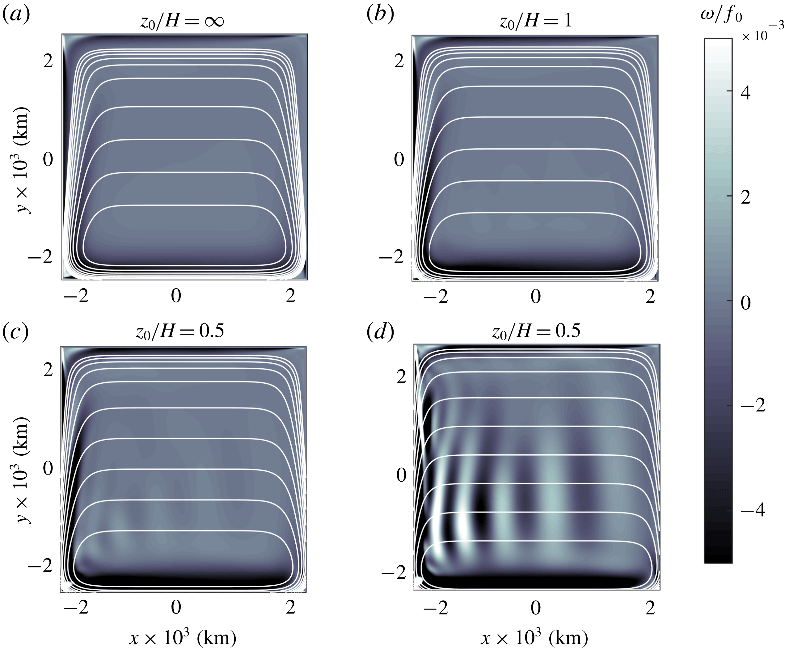
The vorticity fields in figure 8 reveal further details of the flow evolution. For
 $z_{0}/H=1$
(panel b) the western flow is more intense and detaches from the wall at a more northern latitude in comparison with the homogeneous case. In contrast, for shallower equivalent depths (panels c,d), the flow is decomposed in meridional bands with positive and negative vorticity values, characteristic of Rossby waves. The train of waves travels westward along the
 $f/F$
isolines located at
 $y\approx -1000$
km. The phase speed is approximately
 $0.39~\text{m}~\text{s}^{-1}$
(estimated by measuring the speed of a wave crest at the centre of the domain, which travels 850 km in 25 days, approximately). This number agrees quite well with the phase speed of a westward-travelling Rossby wave
 $\unicode[STIX]{x1D6FD}/k^{2}\approx 0.37~\text{m}~\text{s}^{-1}$
, where the wavenumber
 $k$
is calculated with the wavelength of the oscillation (
 $850$
km).
The results in figures 7 and 8 are explained as follows. For
 $z_{0}/H=1$
(figures 7
b and 8
b), the flow behaves in a similar fashion as the homogeneous case because its vertical structure does not depart dramatically from the uniform structure. Thus, the large anticyclone drifts southward until reaching a steady state. As for the homogeneous case, the balance in the vorticity equation is between the topographic,
 $\unicode[STIX]{x1D6FD}$
, forcing and bottom friction terms
 $$\begin{eqnarray}J\left(\frac{f_{0}}{F},\unicode[STIX]{x1D713}\right)-\frac{\unicode[STIX]{x1D6FD}}{F}\frac{\unicode[STIX]{x2202}\unicode[STIX]{x1D713}}{\unicode[STIX]{x2202}x}=\frac{1}{\unicode[STIX]{x1D70C}_{0}}\unicode[STIX]{x1D735}\times \frac{\unicode[STIX]{x1D749}_{s}}{F}-R\left(\frac{1}{F}-\frac{1}{H}\right)\left(-\frac{1}{F}\unicode[STIX]{x1D6FB}^{2}\unicode[STIX]{x1D713}+\frac{1}{F^{2}}\unicode[STIX]{x1D735}F\boldsymbol{\cdot }\unicode[STIX]{x1D735}\unicode[STIX]{x1D713}\right).\end{eqnarray}$$
This balance is equivalent to (4.4), but now with coefficients depending on the derivatives of
 $F$
, instead of
 $h$
, and reduced bottom friction.
For
 $z_{0}/H=0.5$
and 0.25 (panels c,d in figures 7 and 8) the solutions behave differently because of three reasons. First, the influence of the topographic slopes is greatly reduced due to the vertical structure of these flows. As a result, the southward drift of the large-scale gyre is inhibited. Second, as
 $F$
decreases, bottom friction is also reduced because of the factor
 $(1/F-1/z_{0})$
. Lower friction is physically plausible since the flow motion is weaker near the bottom (due to its vertical decay). Third, the effects of the wind are enhanced because the forcing term is proportional to
 $1/F$
. Even though the wind stress is the same, the applied force over a shallower layer is greater than over the whole fluid depth. These three effects impede the flow to reach a steady balance as in the Stommel problem because the forcing and topographic terms cannot be balanced with the
 $\unicode[STIX]{x1D6FD}$
term. As a consequence, the anticyclonic gyre is transformed into a set of planetary waves.
5 The Campeche cyclone
The problem to examine in this section concerns a semi-permanent cyclonic circulation observed in the Bay of Campeche at the southern Gulf of Mexico. This feature is often referred to as the Campeche cyclone, and several studies have documented its surface structure and seasonal occurrence (see e.g. Vázquez de la Cerda et al. (Reference Vázquez de la Cerda, Reid, DiMarco and Jochens2005)). This problem is chosen because it is one of the few oceanic systems (besides the ACC) that presents a barotropic vertical structure, according to averaged current-meter measurements along the water column reported by Perez-Brunius et al. (Reference Perez-Brunius, García-Carrillo, Dubranna, Sheinbaum and Candela2013). The authors estimated an exponential profile with a reference depth of
 $z_{0}=650$
m. Here we explore the generation of the cyclone under the equivalent-barotropic dynamics.
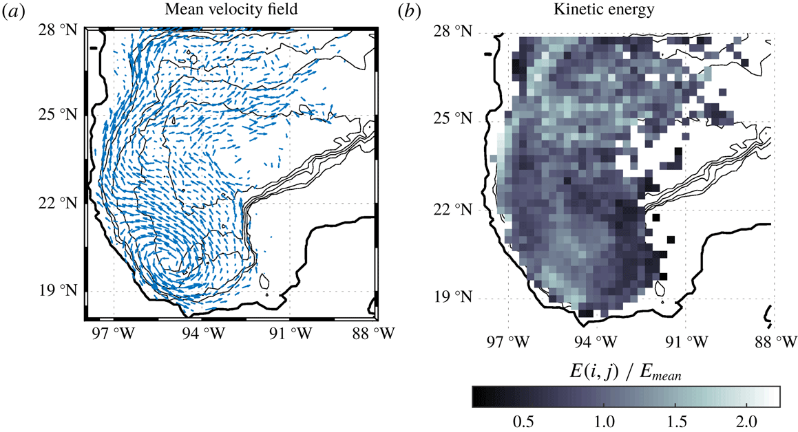
(a) Velocity field in the western Gulf of Mexico calculated from the velocity records of 441 surface drifters during a 7 year period (see text). Maximum velocity is
 $0.36~\text{m}~\text{s}^{-1}$
. (b) Kinetic energy in each geographical bin
 $(i,j)$
, normalised with the mean value of all records
 $E_{mean}=0.0629~\text{m}^{2}~\text{s}^{-2}$
. Topography contours (0, 200, 500, 1500, 2500 and 3500 m) are denoted with thin black lines.
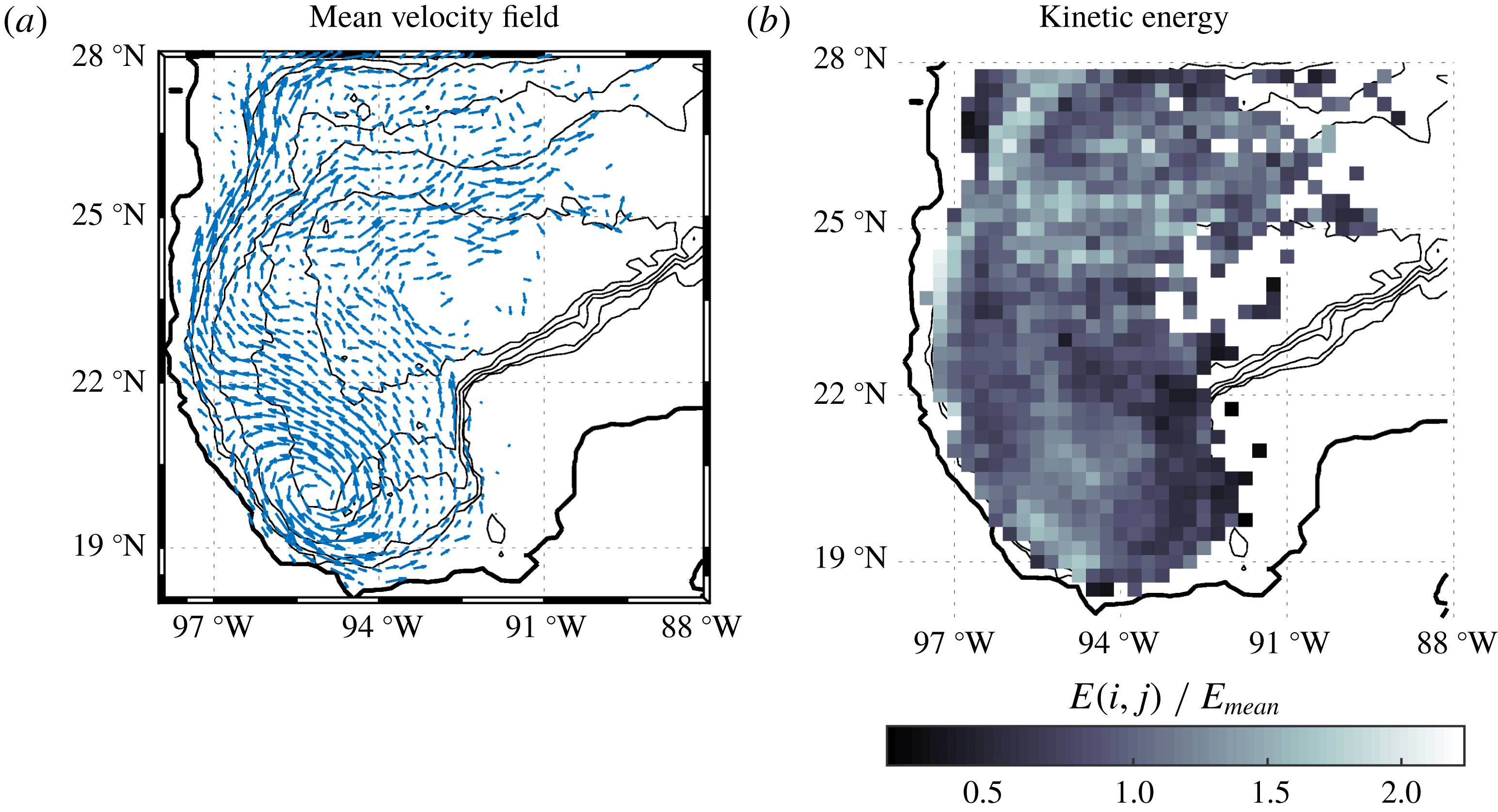
Figure 9(a) presents the western Gulf of Mexico over an area of
 $10^{\circ }\times 10^{\circ }$
. The deepest part is approximately 4000 m. The Bay of Campeche is located at the southernmost part, approximately between [
 $98\,^{\circ }\text{W},91\,^{\circ }\text{W}$
] and [
 $18\,^{\circ }\text{N},22\,^{\circ }\text{N}$
]. The panel also presents the mean surface velocity in a regular grid with resolution of
 $0.25^{\circ }$
. The field was interpolated from the velocity records of 441 surface drifters released in the Bay of Campeche between September 2007 and August 2014 (Perez-Brunius et al.
Reference Perez-Brunius, García-Carrillo, Dubranna, Sheinbaum and Candela2013; Zavala Sansón, Pérez-Brunius & Sheinbaum Reference Zavala Sansón, Pérez-Brunius and Sheinbaum2017). The climatological signature of the Campeche cyclone is the elongated structure along the NW–SE direction at the south-western part of the bay. Note that there are no data over the shallow Yucatan shelf to the east, because the circulation is strongly constrained by the shelf break that starts at about 200 m (shallowest contour). Figure 9(b) shows the kinetic energy field normalised with the mean value of the whole velocity records. The highest values correspond to the cyclone at the south, the northern region and the western margins. Further details of these and other Lagrangian measurements are reported in Zavala Sansón et al. (Reference Zavala Sansón, Pérez-Brunius and Sheinbaum2017) and Zavala Sansón, Sheinbaum & Pérez-Brunius (Reference Zavala Sansón, Sheinbaum and Pérez-Brunius2018).
The causes that generate the cyclone are still open to debate. The most likely candidates are the wind forcing (Gutiérrez de Velasco & Winant Reference Gutiérrez de Velasco and Winant1996; Vázquez de la Cerda et al.
Reference Vázquez de la Cerda, Reid, DiMarco and Jochens2005), eddy-driven vorticity fluxes (Ohlmann et al.
Reference Ohlmann, Niiler, Fox and Leben2001) and the confinement effect of the topography (Perez-Brunius et al.
Reference Perez-Brunius, García-Carrillo, Dubranna, Sheinbaum and Candela2013). The present analysis consists of performing equivalent-barotropic simulations of the wind-driven flow with realistic topography. By using different values of the reference depth
 $z_{0}$
, the possible formation of the Campeche cyclone is explored.
5.1 Flow parameters
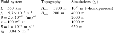
Flow parameters in the simulations of the wind-driven flow in the Gulf of Mexico. The spatial resolution is
 $257\times 257$
grid points and the time step
 $\text{d}t=3600$
s. The Coriolis parameter is calculated at
 $23\,^{\circ }\text{N}$
.
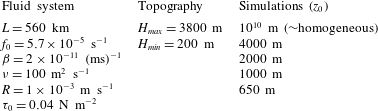
Table 3 summarises the main parameters. The side length of the square domain is
 $2L=1120$
km, which approximately corresponds to the
 $10^{\circ }\times 10^{\circ }$
area shown in figure 9 [
 $98{-}88\,^{\circ }\text{W},18{-}28\,^{\circ }\text{N}$
]. The depth field is linearly interpolated and smoothed from a
 $5^{\prime }$
bathymetric map into a
 $257\times 257$
regular grid, so the spatial resolution is about 4.4 km. Over the continental shelves (between the shelf break at the 200 m contour and the coast), the vorticity-transport function equation cannot be solved because the fluid depth becomes very small. To circumvent this problem,
 $h$
is set to a constant value of 200 m, the forcing is null, and the bottom friction is increased a factor of 100 in coastal regions. This procedure prevents unrealistically high velocities over the shelf and maintains numerical stability, to the cost of underestimating the flow over shallow waters. Thus, the primary interest is focused on solving the flow over deep regions (
 $h>200$
m), where the dominant structures are formed, which is also justified by considering that the exchange between deep and shallow waters is rather weak (as shown in figure 9). On land, the transport function is prescribed to be zero. The lateral boundaries are free slip (part of the northern and eastern walls). The bottom friction coefficient,
 $R$
, is the average value used in some of the simulations by LaCasce & Isachsen (Reference LaCasce and Isachsen2010).
The wind stress is steady, zonally uniform and directed westward. The latitudinal profile is taken as a simple sine function
 $$\begin{eqnarray}\unicode[STIX]{x1D749}_{s}=(\unicode[STIX]{x1D70F}^{x},\unicode[STIX]{x1D70F}^{y})=\left(-\unicode[STIX]{x1D70F}_{0}\sin \left[\frac{\unicode[STIX]{x03C0}}{2L}(y+L)\right],0\right).\end{eqnarray}$$
The flow starts from rest and the external forcing is gradually applied (as in expression (4.3)). The wind jet is maximum at
 $23^{\circ }$
, the centre of the domain, so the southern (northern) region has a positive (negative) wind-stress curl. This structure and its magnitude
 $\unicode[STIX]{x1D70F}_{0}$
are a simplified description of the climatological winds described by Gutiérrez de Velasco & Winant (Reference Gutiérrez de Velasco and Winant1996). The existence of a positive curl at the south suggests that the wind may promote the formation of the Campeche cyclone, as we shall see below.
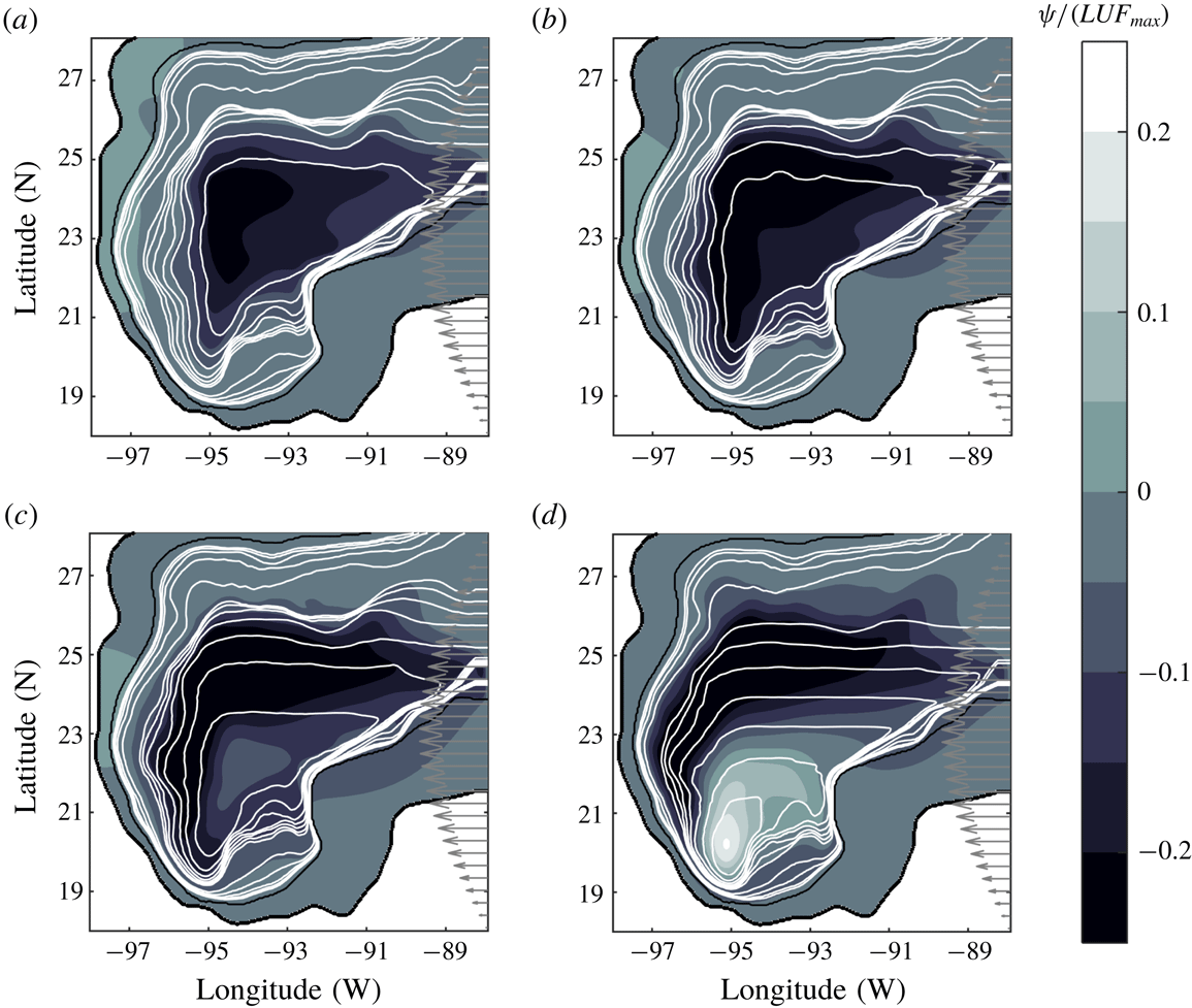
5.2 Conditions for the cyclone formation
Transport function field at
 $t=90$
days in four simulations of the wind-driven flow in the Gulf of Mexico: (a)
 $z_{0}/H=\infty$
, (b)
 $z_{0}=4000$
m, (c)
 $z_{0}=2000$
m, (d)
 $z_{0}=1000$
m. The flow parameters are given in table 3. The r.m.s. speed in each panel is
 $U=[0.002,0.003,0.005,0.012]~\text{m}~\text{s}^{-1}$
, and the maximum equivalent depth
 $F_{max}=[3800,2453,1701,978]$
m. Maximum speeds are
 $U_{max}=[0.106,0.121,0.140,0.153]~\text{m}~\text{s}^{-1}$
. Grey arrows at the eastern side represent the westward wind stress. Black lines indicate the coast and the 200 m isobath. White curves are the
 $(f_{0}+\unicode[STIX]{x1D6FD}y)/F(x,y)$
contours: small contour values at deep regions are
 $[5.362:0.1703:6.383]\times 10^{-8}~(\text{ms})^{-1}$
; large contour values (near the 200 m isobath) are
 $[6.55:1.703:13.36]\times 10^{-8}~(\text{ms})^{-1}$
.
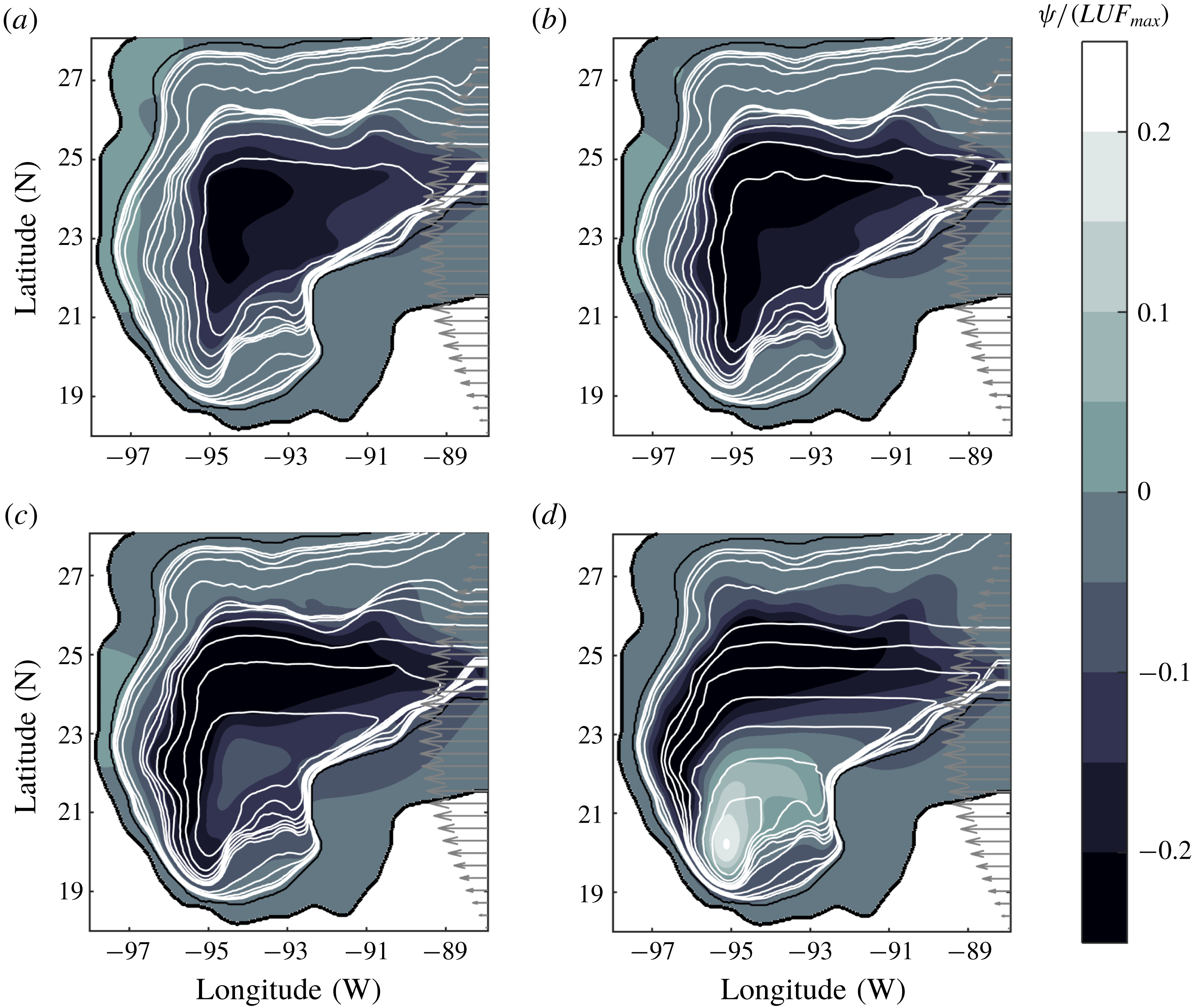
To determine whether the Campeche cyclone is formed under the equivalent-barotropic dynamics, we start with four simulations with
 $z_{0}$
given in the third column of table 3. Figure 10 presents the transport function and the velocity fields at
 $t=90$
days, a time at which the flow has reached a more or less steady state. Note that these examples are analogous to the experiments discussed in previous subsections: the first panel is the result for a homogeneous ocean (
 $z_{0}\rightarrow \infty$
), while the reference depth is progressively smaller in subsequent panels. In the first two cases (a,b) there is the development of an anticyclonic circulation that covers most of the gulf along the geostrophic contours
 $f/F$
. This circulation is due to the negative wind-stress curl over the northern area of the domain. The quasi-homogeneous case (
 $z_{0}=4000$
m, panel b) is more intense because the effects of the forcing are increased whilst those of the bottom friction are decreased, as we saw in previous examples (maximum speeds are shown in the figure caption). These results suggest that the applied forcing is not able to generate a cyclone in the Bay of Campeche when the vertical profile is almost uniform. As
 $z_{0}$
is further reduced to 2000 and 1000 m (panels c,d), the geostrophic contours are closed and shifted southward. Inside these contours, a cyclonic circulation is generated under
 $22\,^{\circ }\text{N}$
(panel d). This is a strong indication that a cyclonic circulation may be generated in the Bay of Campeche when the reference depth is of the order of 1000 m.
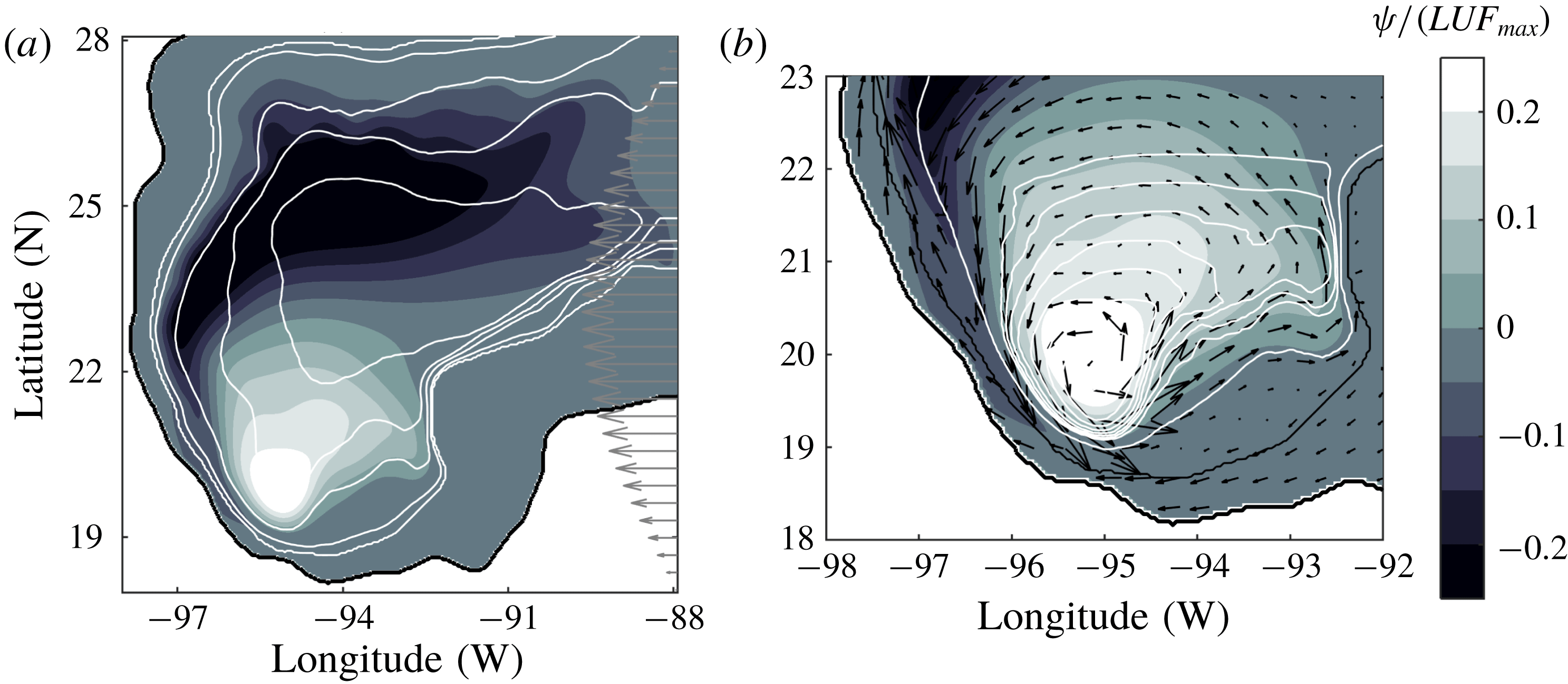
Transport function field at
 $t=90$
days in the Gulf of Mexico with
 $z_{0}=650$
m. (a) Whole domain as in figure 10. The r.m.s. speed is
 $U=0.021~\text{m}~\text{s}^{-1}$
, and the maximum equivalent depth
 $F_{max}=640$
m. Topography contours (0, 200, 500, 1500, 2500 and 3500 m) are denoted with thin white lines. (b) Transport function and velocity field over the Bay of Campeche. Maximum speed is
 $U_{max}=0.124~\text{m}~\text{s}^{-1}$
. White lines indicate the geostrophic contours
 $(f_{0}+\unicode[STIX]{x1D6FD}y)/F(x,y)$
shown in Perez-Brunius et al. (Reference Perez-Brunius, García-Carrillo, Dubranna, Sheinbaum and Candela2013):
 $[(7.8:0.1:8.5),9.5]\times 10^{-8}~(\text{ms})^{-1}$
. Black lines indicate the coast and the 200 m isobath.
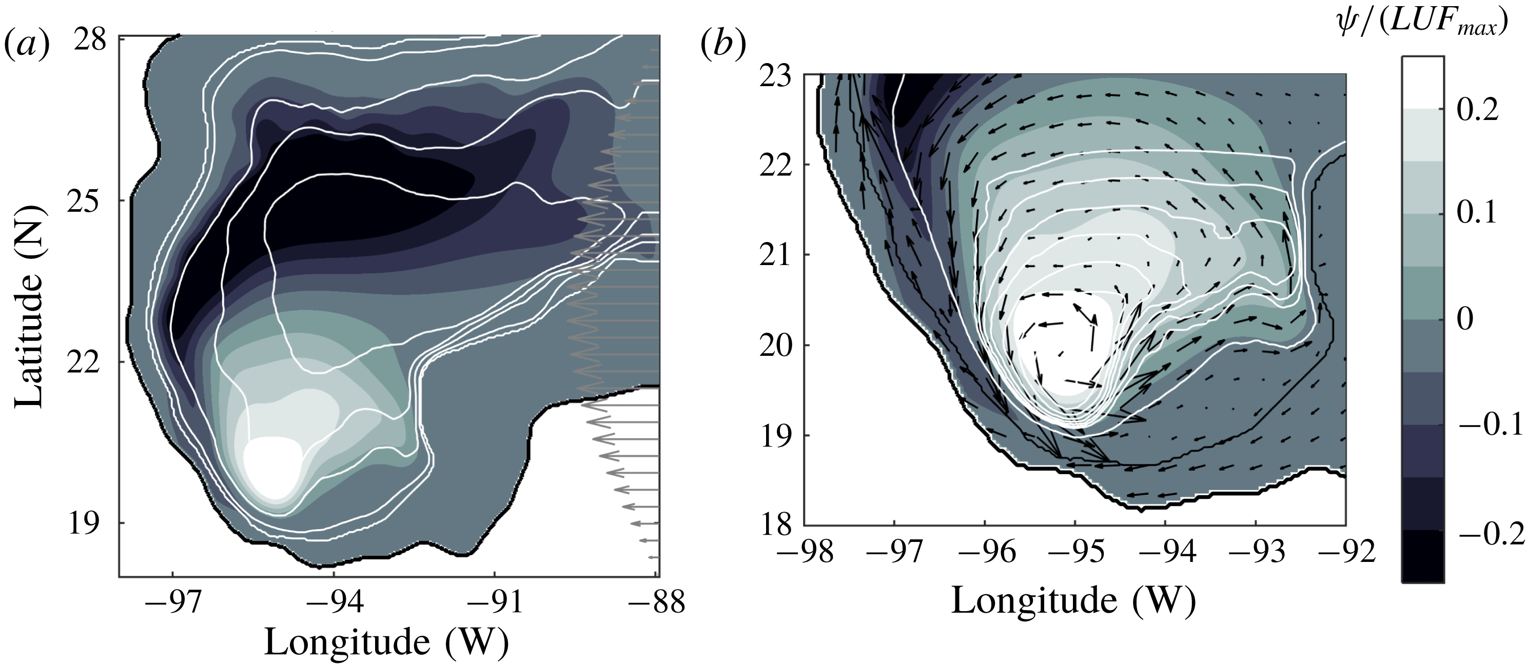
Now we can examine a simulation with the reference depth of 650 m estimated in the observations of Perez-Brunius et al. (Reference Perez-Brunius, García-Carrillo, Dubranna, Sheinbaum and Candela2013). Figure 11(a) shows the transport function and the velocity field superposed with the topography contours. The result is a cyclonic vortex in the Bay of Campeche, which is very similar to the observed structure presented in figure 9(a). The maximum speed measured in the numerical cyclone is
 $0.142~\text{m}~\text{s}^{-1}$
, which is somewhat weaker than the maximum value in the observations (
 $0.36~\text{m}~\text{s}^{-1}$
). In figure 11(b) we plot the same dynamical field but now in a subdomain that encloses the Bay of Campeche, superposed with the velocity field and the geostrophic contours
 $f/F$
. The shape of the contours explains the position reached by the numerical cyclone, as the resulting flow tends to follow these isolines. Thus, the simulations support the generation of the Campeche cyclone due to the positive wind-stress curl at the southern part of the Gulf of Mexico. Moreover, the structure is topographically confined according to the shape of the geostrophic contours.
6 Summary and discussion
We discussed the derivation and the limitations of the equivalent-barotropic dynamics for rotating flows over variable topography. Then, the governing equations were numerically solved in three different problems. The advantages and shortcomings of the formulation and the applications are discussed separately.
6.1 The model
The main feature addressed in this paper is the consideration of time-dependent, nonlinear, barotropic flows with vertical structure
 $P(z)$
and variable depth
 $h(x,y)$
due to bottom topography. This approach is in contrast with oceanic models used in previous studies of the ACC, which are linear and time independent (Gille Reference Gille1995; Krupitsky et al.
Reference Krupitsky, Kamenkovich, Naik and Cane1996; LaCasce & Isachsen Reference LaCasce and Isachsen2010). Those formulations were justified according to the scales of motion of the problem and, certainly, they provided valuable information. Here, we discussed the equivalent-barotropic dynamics of nonlinear flows in laboratory scales and the time evolution of oceanic, wind-driven gyres.
The flow evolution is governed by (2.19)–(2.20) for inviscid, unforced systems with surface relative vorticity
 $\unicode[STIX]{x1D714}_{s}$
and transport function
 $\unicode[STIX]{x1D713}$
. The vorticity equation with forcing and dissipation is (2.26). The dynamical model is identical to that of a homogeneous flow with uniform vorticity
 $\unicode[STIX]{x1D714}_{s}$
over a depth field
 $F(x,y)$
, which is the concept of an equivalent-barotropic system (Charney Reference Charney1949; Killworth Reference Killworth1992). Such idea relies on the assumption of steady, geostrophic flow at every vertical level (Killworth Reference Killworth1992). Therefore the nonlinear model must be regarded as an approximation because the separable form of the variables (2.1) is not consistent with the advective terms in the original vorticity equation (2.13). The mathematical consistency is subject to the smallness of the maximum error (2.18) introduced in the vertically integrated dynamical equation. Thus, the approximation requires weak vertical structures
 $P(z)$
such that
 $1-G/F$
be small pointwise. The nonlinear model derived by Charney (Reference Charney1949) dealt with the same problem. Charney considered a barotropic atmosphere defined by a pressure-dependent vertical structure
 $A(p)$
. The resulting vorticity equation was equivalent to (2.16) but applied at an intermediate level instead of the surface (and using a tendency equation for the horizontal divergence). The factor multiplying the nonlinear terms was a function
 $K=\int A^{2}\,\text{d}p/\int A\,\text{d}p$
equivalent to
 $G/F$
. Then, Charney assumed
 $K\approx 1$
according to available observations and argued that the error should be small.
In the numerical examples, we used the vertical structure
 $P(z)=\text{e}^{z/z_{0}}$
(Gille Reference Gille1995), but different functions may be considered as long as they satisfy the conditions (2.2). In addition, it would be required to examine the vorticity equation, as we did for the exponential function. The critical term is the vertical advection
 $w\unicode[STIX]{x1D714}_{z}$
, which involves both the integral and the derivative of
 $P(z)$
, as shown by (2.14). The consistency of the model depends on the combination of this term and the advective and stretching
 $P^{2}$
terms. The selection of an appropriate
 $P(z)$
also depends on the vertical structure observed in a real system. The exponential profile has been reported in several studies, as discussed above, but the inaccuracy of field observations opens the possibility to consider other vertical structures. Therefore further investigations with different functions may be worthwhile in future studies.
Simplified parametrisations were used to include forcing and dissipation terms in the vorticity equation (2.26). For instance, turbulent viscous effects are chosen as a standard Laplacian term, and bottom friction is proportional to the relative vorticity, equivalent to linear Ekman friction (Zavala Sansón & van Heijst Reference Zavala Sansón and van Heijst2002). The wind stress is the same as that used in previous studies (Krupitsky et al.
Reference Krupitsky, Kamenkovich, Naik and Cane1996; LaCasce & Isachsen Reference LaCasce and Isachsen2010). The parametrisations capture two physical effects that are expected when using a shallow equivalent depth
 $F$
. First, the transfer of momentum due to the forcing term is increased with respect to the homogeneous case, because now the wind-stress acts over a shallower fluid layer. Second, the bottom friction term is reduced because the bottom stress is less effective over the moving fluid near the surface. The combination of these two effects implies that a stratified flow will experience a greater forcing at the surface and reduced bottom friction so that the resulting horizontal flow will be more energetic.
6.2 The simulations
To examine the equivalent-barotropic dynamics over variable topography, we studied numerically three problems that illustrate the role of nonlinear effects and the long-term behaviour of time-dependent flows. The simulations included two well-validated limits: a purely barotropic flow with topography (when the reference depth
 $z_{0}\rightarrow \infty$
) and a nearly 2-D flow (as
 $z_{0}$
becomes small and the topography is smoothed out). It is inferred that if the model reproduces well these two limiting dynamics, then the intermediate cases illustrate the effects of the vertical structure (with the assumption that the flow remains barotropic).
First, the topographically induced drift of a cyclonic vortex around a seamount was studied. This example was chosen because it is highly nonlinear. There is no external forcing, and bottom friction effects play a secondary role. In the homogeneous case, a vigorous vortex turns around the mountain in the clockwise sense, while a patch of negative vorticity is formed on the summit due to squeezing effects (Zavala Sansón et al.
Reference Zavala Sansón, Barbosa Aguiar and van Heijst2012). When the flow has a vertical structure, the equivalent depth is progressively smoothed as the parameter
 $z_{0}/H$
decreases. As a result, the revolutions of the vortex around the mountain are reduced because the topographic influence is also reduced. For the shallowest
 $F$
, the vortex barely drifted. Thus, the model effectively isolates the upper flow region from topographic effects, as expected for a stratified flow.
The second example concerned the Stommel problem with topography, which consists of wind-driven flow on a
 $\unicode[STIX]{x1D6FD}$
-plane, enclosed in a basin with variable topography and bottom friction. The flow is mostly linear, and the aim was to observe the long-term configuration for different
 $z_{0}/H$
values. Starting from rest, the flow evolves towards a large-scale anticyclonic gyre (according to the uniform, zonal wind with negative curl), intensified at the western wall, as in the classical Stommel problem over a flat bottom. For a homogeneous system, the flow tends towards a steady state in which the
 $\unicode[STIX]{x1D6FD}$
-effect, the wind-stress curl, the linear friction and the topographic terms are balanced in the vorticity equation. The difference with the Stommel problem is that the large anticyclonic circulation is shifted southward along the western wall, due to the influence of the topographic slope (Salmon Reference Salmon1998). When using a shallower equivalent depth
 $F$
, the southward shift of the gyre is reduced because the topographic effect is also reduced. For even shallower
 $F$
, the large-scale circulation is decomposed as Rossby waves travelling in the zonal direction. Also, the bottom friction is reduced, making the Stommel balance impossible to achieve. As a consequence, the flow becomes unsteady as planetary waves are radiated.
Several aspects of the Stommel problem may be further investigated to determine the relevance of the topographic variations against the thickness of the upper active region. For instance, the flow detachment from the western boundary along the
 $f/F$
contours, and the shape of the bottom topography with either closed or open geostrophic contours, are relevant issues for the flow dynamics (LaCasce & Isachsen Reference LaCasce and Isachsen2010). Also, details of the generated Rossby waves remain to be understood, such as the latitude of propagation. The results are part of a different study to be published somewhere else.
Finally, we examined the formation of the Campeche cyclone in the southern Gulf of Mexico (Vázquez de la Cerda et al.
Reference Vázquez de la Cerda, Reid, DiMarco and Jochens2005; Perez-Brunius et al.
Reference Perez-Brunius, García-Carrillo, Dubranna, Sheinbaum and Candela2013). The simulations were simplified in the sense that (i) bottom topography is realistic though smoothed and (ii) the applied wind-stress curl is uniform over the domain, having a similar distribution and magnitude as the climatological values (Gutiérrez de Velasco & Winant Reference Gutiérrez de Velasco and Winant1996). When the flow is barotropic (or nearly), the dominant circulation was a large-scale anticyclonic cell over most of the region. In other words, the applied forcing was unable to generate a cyclonic structure at the southern part, even though the wind-stress curl is positive over this region. In contrast, as the reference depth
 $z_{0}$
was reduced, the formation of a cyclone became evident. Moreover, when using
 $z_{0}=650$
m, as proposed by Perez-Brunius et al. (Reference Perez-Brunius, García-Carrillo, Dubranna, Sheinbaum and Candela2013), the resemblance of the cyclonic vortex with the Campeche cyclone was remarkable. Our main conclusion is that the formation of a topographically confined, positive circulation over the Bay of Campeche is compatible with the equivalent-barotropic dynamics.
It is emphasised that the present simulations are not intended to reproduce observational data, but rather to shed light on the physical mechanisms that promote the formation of an oceanic structure, whose origins to this day are not well understood. A more detailed analysis would be required to examine the influence of the forcing function (by considering spatial variations, small-scale perturbations, climatological values, etc.), the size of the numerical domain, the resolution of the bottom topography and, above all, the influence of realistic stratification.
Acknowledgements
Comments and helpful suggestions from J. Vanneste and J. Sheinbaum are gratefully acknowledged. The essential parts of this study were carried out during an academic visit to the University of Edinburgh, UK.