1 Introduction
Flow separations are often associated with increased drag, lift losses, kinetic energy losses and so on; apart from some cases utilizing separated vortices, such as the lift increase of airfoils by detached vortices and decreased losses of diffusers by vortex generators. As a result, many researchers have been preoccupied for almost a century with weakening flow separation or even avoiding it entirely. Flow separations were shown in experiments and in numerical simulations which were unsteady in a wide range of Reynolds number. Although a complex time-dependent coherence of flow separation is seen, it still remains unexploited in most cases. Using the potential of unsteadiness, unsteady flow control or periodic excitation methods were shown to be much more effective than traditional steady flow control methods. They can save one or two orders of magnitude of the momentum injection required to achieve the same performance improvement, resulting in autonomous, small, light, energy-efficient actuators, thereby overcoming most of the deficiencies of traditional control methods (Greenblatt & Wygnanski Reference Greenblatt and Wygnanski2000; Collis et al. Reference Collis, Joslin, Seifert and Theofilis2004). For decades, researchers have engaged in different unsteady flow control methods, such as acoustic excitation (Lepicovsky et al. Reference Lepicovsky, Ahuja, Brown and Morris1986; Nishioka, Asai & Yoshida Reference Nishioka, Asai and Yoshida1987), pulsed jet (Hassan Reference Hassan2004; Gmelin et al. Reference Gmelin, Steger, Wassen, Thiele, Huppertz and Swoboda2010; Hecklau et al. Reference Hecklau, Wiederhold, Zander, King, Nitsche and Swoboda2011), synthetic jet (Glezer & Amitay Reference Glezer and Amitay2002; Amitay & Cannelle Reference Amitay and Cannelle2006; Smith & Glezer Reference Smith and Glezer1998), wall oscillation (Wu, Wu & Wu Reference Wu, Wu and Wu1991; Sinha Reference Sinha1999), and travelling wave wall (Wu, Xie & Wu Reference Wu, Xie and Wu2003; Wu, Wang & Wu Reference Wu, Wang and Wu2007; Chen, Liu & Hu Reference Chen, Liu and Hu2014), achieving good performance improvements.
Currently, unsteady flow control is a fast-growing frontier. Although several related studies have been identified and many of its applications have increased in recent years, an essential understanding of its mechanism and the true optimization of the control strategy seem out of pace with this growth (Wygnanski Reference Wygnanski2004). Possible fragmentation mechanisms of unsteady flow control are scattered over different kinds of literature, while some of the important ones have been restated. First, the effectiveness of periodic excitations is found to be relevant to global flow instability even in turbulence, and periodic addition of the momentum at the appropriate location, magnitude and frequency can interact with the large-scale coherent structures of a flow, using inherent flow instabilities (Collis et al. Reference Collis, Joslin, Seifert and Theofilis2004). Some studies have been conducted using the Rayleigh equation, Orr–Sommerfeld equation (OSE) or Orr–Sommerfeld-like equation for the turbulent flow, analysing the instabilities approximately and quantitatively, as used in studies on acoustic excitation and pulsating jets (Nishioka et al. Reference Nishioka, Asai and Yoshida1987; Skamnakis & Papailiou Reference Skamnakis and Papailiou2005). For a typically separated flow of airfoils or blades, the instabilities lie in the shear layer, separation bubble, wake structures, and their interactions (Ye, Cattafesta & Mittal Reference Ye, Cattafesta and Mittal2006; Gursul, Cleaver & Wang Reference Gursul, Cleaver and Wang2014). Among them, instability of a free shear flow is of great importance and the excited mixing layer is regarded as the basis for unsteady separation control. With theoretical and experimental data on the free shear layer (Dimotakis Reference Dimotakis1989) and the excited free shear layer (Roberts Reference Roberts1985; Wygnanski & Petersen Reference Wygnanski and Petersen1987), it is also argued that the optimum parameters of the excitation are related to neutral stability and the amount of momentum transfer through the coherent structures of mixing flow (known as entrainment) (Greenblatt & Wygnanski Reference Greenblatt and Wygnanski2000; Seifert, Greenblatt & Wygnanski Reference Seifert, Greenblatt and Wygnanski2004). Further analysis of the flow field indicates that effective excitation can make the flow field more orderly, compared with uncontrolled flows or those with inappropriate excitation (Zheng, Zhou & Zhou Reference Zheng, Zhou and Zhou2005). Thus, the keywords related to the mechanisms of unsteady flow control are coherent structures, instability, entrainment, and degree of order, respectively. However, it is obvious that these aspects are merely one-sided or overlap with others, making a globally valid mechanism unclear.
By producing a mass of flow field information to be processed, both the experiments and numerical simulations are difficult to use in exploring the nature of unsteady flow control. As a typical flow phenomenon, the vortex structure of an unsteady separated flow field is complex even without considering the interaction between periodic external excitation and the unsteady separated flow. Most studies consider the details of flow fields as a black box. They rather focus on the contrasting overall flow characteristics in the different control states to analyse the effects of unsteady control (Greenblatt & Wygnanski Reference Greenblatt and Wygnanski2000). However, this method ignores the details, making it difficult to understand the nonlinear mechanisms of unsteady flow control. With such deficiencies in these methods, researchers have sought to enhance understanding of its mechanism and control using more refined numerical and experimental methods, which can produce high-accuracy unsteady flow fields such as unsteady Reynolds-averaged Navier–Stokes simulation (URANS) (Monir, Tadjfar & Bakhtian Reference Monir, Tadjfar and Bakhtian2013), detached-eddy simulation (DES) (Wang, Li & Fu Reference Wang, Li and Fu2014), large eddy simulation (LES) (You & Moin Reference You and Moin2006; Kim Reference Kim2009) and particle image velocimetry (PIV) (Gursul et al. Reference Gursul, Cleaver and Wang2014). On one hand, numerical simulations of unsteady flow fields use excessive computer resources, while experiments with many gauging points cost a lot of money. On the other hand, the mass of information on unsteady flow fields is difficult to process to extract the essential laws of a mechanism which can be captured and applied effectively. With a huge quantity of data generated by these high-accuracy numerical or experimental methods, several flow data processing methods have arisen, such as proper orthogonal decomposition (POD) (Chatterjee Reference Chatterjee2000; Gross Reference Gross2005) and dynamic mode decomposition (DMD) (Schmid Reference Schmid2008; Schmid et al. Reference Schmid, Li, Juniper and Pust2010). But the unsteady separated flows are complex and involve various trans-scale flow structures (Lumley Reference Lumley1967; Chatterjee Reference Chatterjee2000). It is extremely difficult to discover the mechanism of interactions between separated flows and the controlling excitation from the complex experimental and numerical results. Flow data processing methods, such as POD, can only be used to obtain some final difference of the flow fields between the controlled and uncontrolled flows. They face difficulties in displaying any detailed information about the evolution from uncontrolled separated flows to controlled flows.
In history, as classic methods, models are commonly used to simplify and solve complex problems in fluid mechanics. Based on the Navier–Stokes equation (N–S equation) and linear perturbation theory, the OSE (Orszag Reference Orszag1971) is widely used for stability analysis, including the laminar–turbulent transition of flat plate flow and shear flow. Different types of OSE have been presented, respectively, from easy to difficult: two-dimensional (2D) inviscid parallel OSE (Rayleigh equation) (Miles Reference Miles1962), 2D viscous parallel OSE (Gaster & Jordinson Reference Gaster and Jordinson1975; Grosch & Salwen Reference Grosch and Salwen1978), 2D non-parallel OSE (Dušek, Fraunié & Gal Reference Dušek, Fraunié and Gal1994), and 3D non-parallel OSE (Theofilis Reference Theofilis2003). Nevertheless, to make the OSE linear, a hypothesis of small perturbations was made initially, resulting in failure of the OSE in the presence of nonlinear phenomenon, such as saturation of perturbation. To partially address this issue, a weakly nonlinear model, the Stuart–Landau equation (SLE) was proposed and deduced by Landau and Stuart. The SLE was mostly used to model supercritical bifurcations occurring in flow systems when a parameter is within the vicinity of a critical value – a typical example being the transition from steady flow to vortex shedding in the wake of a circular cylinder (Stuart Reference Stuart1958; Thompson & Gal Reference Thompson and Gal2004). This model was then extended to forced SLE to describe wake flows from forced or freely oscillating bodies, showing more nonlinear phenomena such as bifurcation, frequency locking, and hysteresis, apart from the bifurcation and saturation that are already reflected by the original SLE (Olinger Reference Olinger1993; Gal, Nadim & Thompson Reference Gal, Nadim and Thompson2001; Sun Reference Sun2002). The SLE also provides a starting point for the Ginzburg–Landau model (GLM), which describes further phenomena of 2D shedding from a circular cylinder (Albarè & Provansal Reference Albarè and Provansal1995; Thompson & Gal Reference Thompson and Gal2004). Also, the behaviour of a large number of Landau–Stuart oscillators coupled with the mean field has been recently studied. It has been observed that the macroscopic dynamics of the mean field can be chaotic (Ku, Girvan & Ott Reference Ku, Girvan and Ott2014). Also, the van der Pol equation, a close relative of SLE and GLM, was used to model transient and steady-state flow over a stationary or forced cylinder (Skop & Balasubramanian Reference Skop and Balasubramanian1995; Nayfeh et al. Reference Nayfeh, Marzouk, Arafat and Akhtar2005). This was modified by adding a cubic term (changing to van der Pol–Duffing oscillator) or an axial diffusion term to extend its application to elliptic cylinders or shear flows (Skop & Balasubramanian Reference Skop and Balasubramanian1995; Akhtar, Marzouk & Nayfeh Reference Akhtar, Marzouk and Nayfeh2009a ). Currently, it is widely accepted that whereas linear stability theory is relatively mature, the nonlinear theory is far from mature enough to be applied in strong nonlinear or even chaotic dynamic systems (such as unsteady separated flow), although some weakly nonlinear versions (such as SLE) can describe some particular and simple flow phenomena well.
As cited previously, based on some typical physical flow characteristics, deduced from the N–S equation and conforming to the experimental results, the simplified models discussed initially were relatively strict. Also, the physical flow characteristics selected by these models were too simple, and such models could not represent complex separated flows, especially their chaotic characteristics. On the other hand, a particular approximate simplified model, covering major factors and ignoring minor factors, may avoid the existing difficulties cited earlier, with the aim of revealing the mechanism of unsteady separation control. This showed that the establishment of a suitable approximate simplified nonlinear model was necessary, which could satisfy the known characteristics of the unsteady separated flows with or without external periodic excitation.
In addition, the complexity of unsteady separated flow forces us to approach it from a different point of view. The main flow characteristics and phenomena from the unsteady separated flow field may be extracted, and then some simple key flow structures could be sought and highlighted. A simplified model may be obtained from a simple flow phenomenon by the above approach so as to solve flow separation problems. Even if this modelling method is not as strict as those deduced models, the authenticity of the simplified model could be confirmed by validation with the experimental or numerical results. Also, the simplified modelling method could make it possible to reveal the mechanism of unsteady flow control, which is buried in the miscellaneous flow field data.
2 Establishment of a nonlinear dynamic model for typical flow separation
As already cited, because the inherent instability leads to unstable separated vortical structures, most of the flow separation is in an unsteady state, making the whole flow field very complex. However, in this complex unsteady flow field, there are some orderly coherent structures, such as periodic shedding vortices, so the chaotic coherent phenomenon is the main characteristic of the unsteady flow separation (Aref Reference Aref1987; Saffman Reference Saffman1992). In addition, a previous study shows that effective unsteady flow control drives the vortical structures to be more ordered than the originally separated flows (Zheng et al. Reference Zheng, Zhou and Zhou2005). In conclusion, in the presence of external excitations, the coherent structures and quasi-ordering characteristics of the flow separation will be changed, implying that interactions between unsteady external excitation and separated flow may be a kind of chaotic control behaviour. Therefore, a simplified dynamic chaotic model needs to be established. To accomplish that, unsteady flow separation characteristics are analysed initially. In this paper, the chaotic dynamic mechanism of the simplified nonlinear model is interpreted in two levels as follows.
2.1 Analysis of the primary dynamic mechanism in unsteady flow separation
In general, the separation scenarios are associated with 3D flow, which is different from 2D flow separation topologically. Also, as a simpler phenomenon, 2D flow separation is easier to model and plays an essential role in flow separation without strong 3D effects, such as in 2D airfoils and some sections of compressor blades far away from hub and shroud. Moreover, flow control with a periodic excitation is seen to be more relevant to the Kelvin–Helmholtz (K–H) (Greenblatt & Wygnanski Reference Greenblatt and Wygnanski2000) or bi-global (2D) instability (Collis et al. Reference Collis, Joslin, Seifert and Theofilis2004). Thus, in this paper, the model is aimed at 2D separations, which also restricts its application scope to 2D or 3D separations without a strong 3D effect, to represent their main dynamic characteristics and not try to simulate 3D details and unsteady 3D flow structures although they exist in some real 2D flow separations. The application scope of this model is also closely related to the premises claimed before modelling. The main premises are listed here and the proposed model may apply to actual flow separations consistent with these premises.
-
(i) The flow is characterized by 2D flow separation.
-
(ii) The large-scale coherent structures are mainly caused by 2D instability.
-
(iii) Interaction of the different vortical structures (such as wake and separation interaction) is negligible, and only a single dominant frequency is important in the flow field.
-
(iv) The effect of external excitation is mainly on large-scale coherent structures.
-
(v) The flow loss can be characterized by the large-scale coherent structure, which is indexed to the degree of order in this paper.
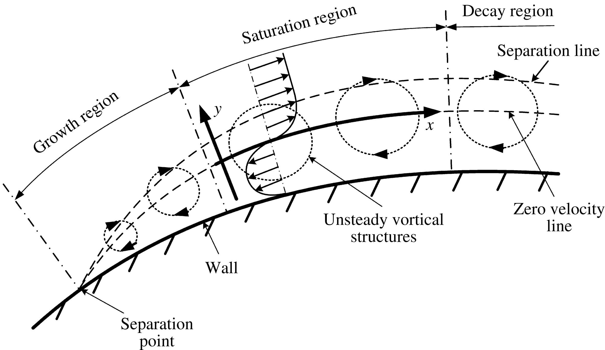
In a typical 2D flow separation near the separation point, the fluid on both sides of the separation point comes from different regions with velocities in opposite directions (figure 1), which is a phenomenon similar to the free shear layer flow formed by two jets flowing in parallel with different velocities (Saffman Reference Saffman1992). Considering the inherently unstable characteristics of the free shear layer, vortices in the shear layer will roll up and move downstream spontaneously. From the stability perspective, and in spite of the vibration of the separation point, separated flow is similar to free shear layer flow, including the chaotic coherent structures generated by the rolled up vortices in the separated flow, as seen in free shear layer flow. In this paper, flow instability is a primary factor that creates coherent structures in both the free shear layer and unsteady flow separation. The characteristics of the shear layer represent the chaotic features in the unsteady separated flow. For simplification, the establishment of the nonlinear model is initially focused on the chaotic characteristics in the free shear layer.
Flow image of large-scale unsteady vortical structures in a separated flow.

The evolution of vortices in the free shear layer consists of rolling up and generation, pairing and merging, and streamwise and spanwise vortex generation processes (Wu, Ma & Zhou Reference Wu, Ma and Zhou2006). The three respective regions related to these three processes are K–H unstable, nonlinear instability, and turbulent regions. When it comes to flow separation we also divided the evolution of the large-scale unsteady vortical structures into three regions, such as growth, saturation, and decay. The vortical structures increase rapidly in the growth region because of flow instability and the increasing height of the separation zone, while they gradually decay as a result of the turbulent dissipation and declining separation zone height. However, there exists a saturation region where the size of vortical structures remains almost the same because of the nonlinear saturation of the flow instability and the almost invariant height of the separation zone. This region is of great importance and modelled in § 2.2.
Based on existing unsteady control results in the free shear layer, it is found that when the external excitation is located at the first two regions where the shear starts, the unsteady control effect is more obvious while in the separated flow, the best excitation location lies near the separatedn point (Dyke Reference Dyke1982; Ho & Huerre Reference Ho and Huerre2003), where the shear origins are found. The similar best excitation locations imply that the separation and free shear layer flows may share the same unsteady control mechanism. So the corresponding nonlinear simplified dynamic model will be established based on the flow characteristics of the free shear layer in the K–H unstable region.
2.2 Free shear layer flow modelling based on analysis of its nonlinear dynamics
In figure 1, when focusing on the saturation region, consider the zero velocity line as the
 $x$
-axis and its orthogonal line as the
 $y$
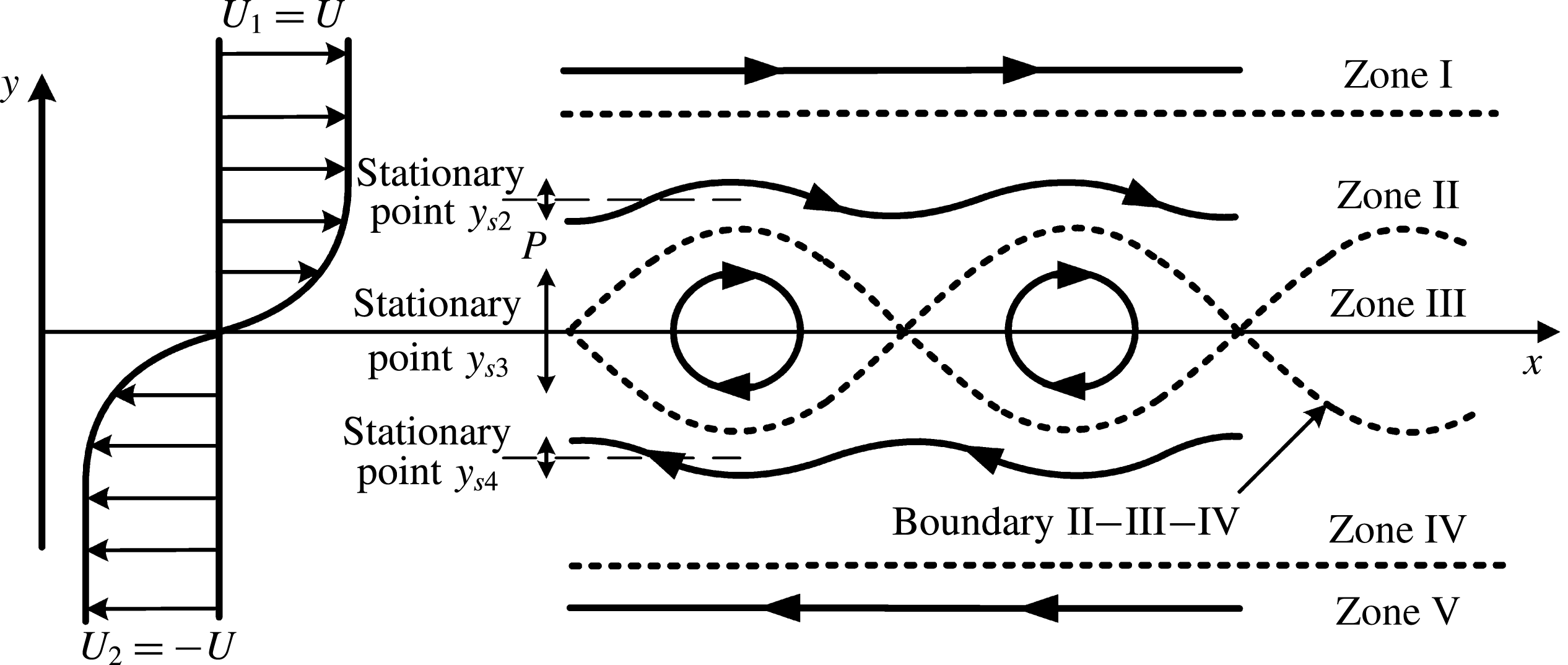
-axis. This part of the separated flow is approximately equivalent to the free shear flow shown in figure 2. The influence of the wall, curved coordinates and so on is ignored in the approximate treatment, to avoid secondary factors. Then we can focus on the free shear layer shown in figure 2.
Because of the K–H instability, the boundary of the free shear layer will roll up and generate co-rotating spanwise K–H vortices, with a final phase speed of approximately
 $(U_{1}+U_{2})/2$
, where
 $U_{1}$
and
 $U_{2}$
represent the velocities of the parallel flow on each side of the shear boundary (Wu et al.
Reference Wu, Ma and Zhou2006). As seen in figure 2, the Stuart vortex row, which is an exact solution of the Euler equation, can be used to approximately describe the large-scale vortex structures in the free shear layer (Stuart Reference Stuart1967; Alobaidi, Smith & Mallier Reference Alobaidi, Smith and Mallier2014). In this case, the relationship
 $U_{1}=-U_{2}=U$
exists and means that the phase speed of the Stuart vortices is zero. This is always possible by coordinate transformation. To further simplify the model, the characteristics of the particle motion are considered, along with the cross-direction (
 $y$
direction, figure 2), instead of the flow direction (
 $x$
direction, figure 2). The flow field can be divided into five zones. Zones I and V are where the flow particle is not affected by the K–H instability. However, Zones II, III, and IV are regions that are strongly dominated by the K–H instability. Considering a particle
 $P$
flowing in these regions, it will fluctuate in the cross-direction as it is strongly driven by the K–H unstable waves and other complex chaotic flow structures. Its motion characteristics can represent the chaotic characteristics in the shear layer flow to a certain extent. Therefore, the authors believed that if the dynamic model of such fluctuation motion along the cross-direction was established, then the intrinsic nonlinear motion of the particles in the free shear layer flow may be described to a certain degree.
Schematic diagram of the Stuart vortex row in a free shear layer.

Apart from the earlier discussion, three general features should be considered before modelling.
-
(1) Source term: The particle
 $P$
fluctuates because of the K–H instability, which means the fluctuant energy of the particle comes from K–H unstable waves, serving as a source term.
-
(2) Dissipation term: Fluid viscosity and small-scale vortices lead to dissipation and restrain fluctuation growth with the same function of damping.
-
(3) Nonlinear term: The amplitude of the K–H unstable wave in a practical flow is often large enough to induce nonlinear effects, rather than the K–H unstable wave theory, which is based on linear perturbation theory, in the free shear layer (Wu et al. Reference Wu, Ma and Zhou2006). Thus, taking into account the corresponding nonlinear effect is inevitable.

Briefly, the K–H unstable wave, dissipation effect, and nonlinear effect, all contribute to the fluctuant movement of particle
 $P$
, and the corresponding terms in the model are known as the source, dissipation, and nonlinear terms. Under the Lagrange method, the fluctuations in the
 $y$
-direction of particle
 $P$
are by analogy with the theory of nonlinear oscillation. Through several simplification and approximation procedures, these three terms can be deduced from the 2D incompressible N–S equation based on Lagrangian coordinates. As we show in appendix A, it is assumed that the viscous and turbulent dissipation is equivalent to linear damping, and the interaction between movements in the
 $x$
-direction and
 $y$
-direction of a particular fluid particle is negligible, then the N–S equation can be simplified as
 $$\begin{eqnarray}\frac{\text{d}^{2}y}{\text{d}t^{2}}=a(t)y+b(t)y^{2}+c(t)y^{3}-K_{d}\frac{\text{d}y}{\text{d}t}+f(t).\end{eqnarray}$$
In the simplified (2.1),
 $a(t)y$
is a linear term, which is not cited before modelling and
 $b(t)y^{2}+c(t)y^{3}$
is the nonlinear term that we are looking for. However, equation (2.1) is non-autonomous because
 $a(t)$
,
 $b(t)$
,
 $c(t)$
and
 $f(t)$
are time-dependent, which means
 $a(t)$
,
 $b(t)$
,
 $c(t)$
and
 $f(t)$
are all source terms, resulting in different energy injections to the dynamic system at different times. With the flow image shown in figure 2, the movement of each flow particle in these five zones can be approximately regarded as uniform rectilinear motion, simple harmonic wave motion, and uniform circular motion. All of these three kinds of flows can be regarded as energy-conservative motions. Thus, pressure gradiant
 $\unicode[STIX]{x2202}p/\unicode[STIX]{x2202}y$
(
 $p$
is pressure here, see appendix A) is independent of time in describing the motions in figure 2 because the system with time-dependent terms is not energy-conservative. Also, the Stuart vortex row is based on the Euler equation, so both viscosity and turbulence are beyond consideration. Then, to model the flow image of the Stuart vortex row shown in figure 2, equation (2.1) can be simplified to
 $$\begin{eqnarray}\frac{\text{d}^{2}y}{\text{d}t^{2}}=ay+by^{2}+cy^{3}+f.\end{eqnarray}$$
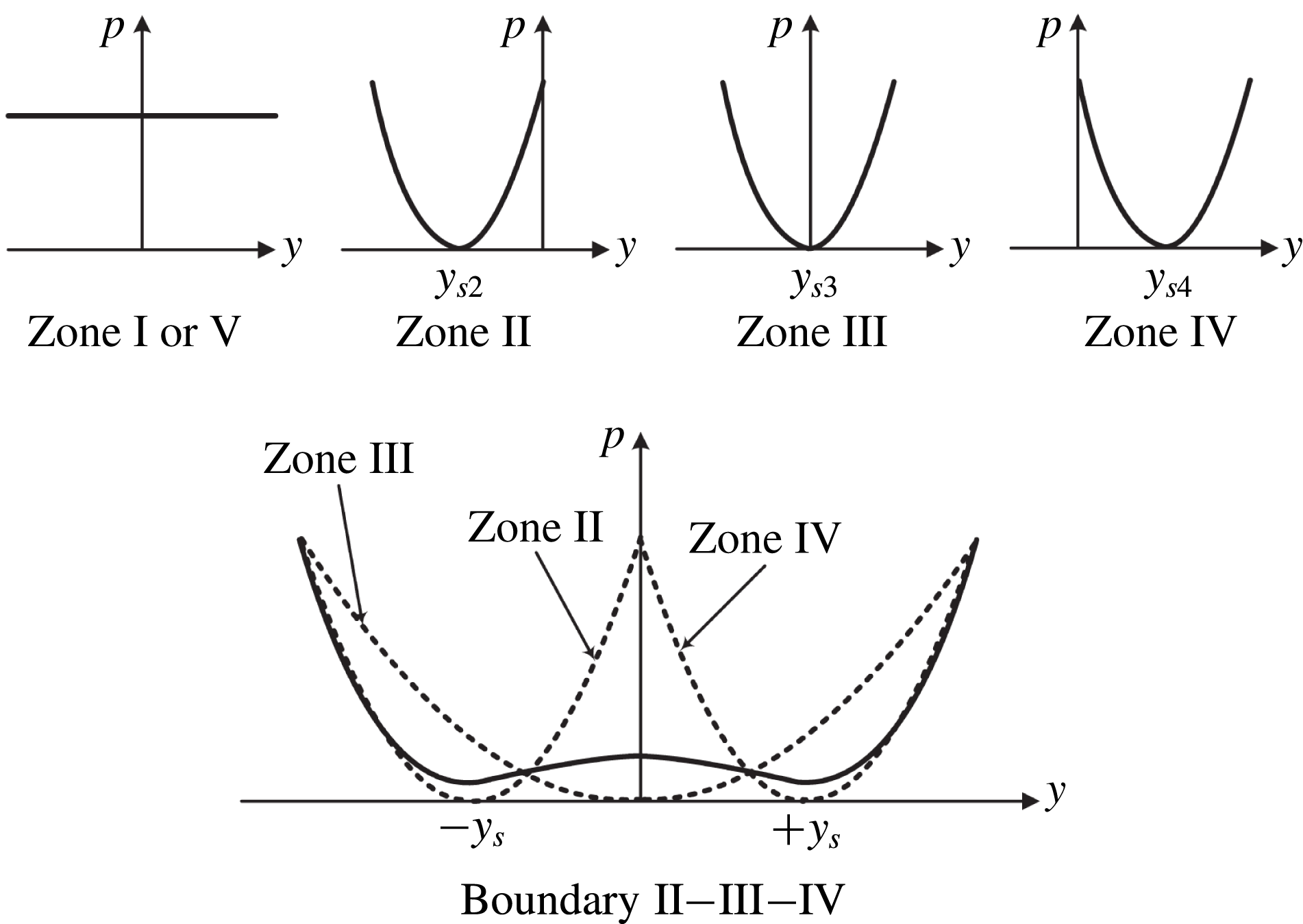
Now, equation (2.2) can be applied to the five zones in figure 2. The flow image shown in figure 2 is symmetric, which simplifies the analysis to a certain degree. As cited earlier, the movement of flow particles in these five zones can be approximately regarded as uniform rectilinear motion, simple harmonic wave motion, and uniform circular motion. Also, it is assumed that the pressure distribution of Boundary II–III–IV is in between that of Zones II, III, and IV. For detailed discussions of these zones and the boundary, see appendix B. As shown in appendix B, without the dissipation term, the
 $y$
-direction motion of fluid particles in the vicinity of Boundary II–III–IV can be approximately expressed as
 $$\begin{eqnarray}\frac{\text{d}^{2}y}{\text{d}t^{2}}=\unicode[STIX]{x1D700}\unicode[STIX]{x1D714}_{0}^{2}y-\frac{\unicode[STIX]{x1D700}\unicode[STIX]{x1D714}_{0}^{2}}{y_{s}^{2}}y^{3},\end{eqnarray}$$
where
 $\unicode[STIX]{x1D714}_{0}$
is the characteristic frequency of the Stuart vortex,
 $\pm y_{s}$
are two stable equilibrium points (see figure 2), and
 $\unicode[STIX]{x1D700}=0.818$
(see appendix B for more details).
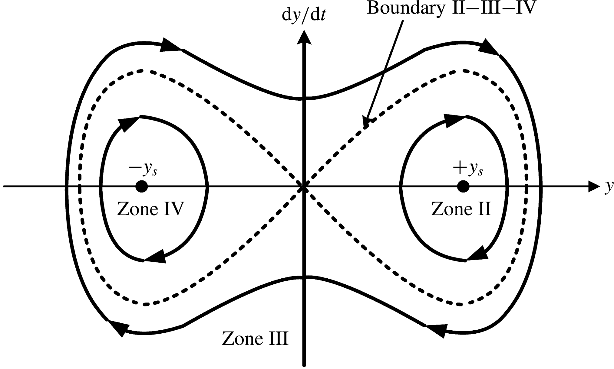
This is a common conservative Duffing equation with a negative linear positive cubic stiffness (Kovacic & Brennan Reference Kovacic and Brennan2011). The relationships between the coefficients of the linear and cubic terms are constrained by this work (see (2.3)). From its phase portrait, which is shown in figure 3, it can be seen that the zones and the boundary correspond with those in figure 2, respectively. For example, the fluid particle oscillating around the stationary point
 $y_{s2}$
in Zone II, as shown in figure 2, corresponds with the phase portrait around
 $+y_{s}$
in Zone II, as shown in figure 3. Also, the fluid particle oscillating around the stationary point
 $y_{s3}$
in Zone III, as shown in figure 2, corresponds with the phase portrait around the zero point (
 $y=0$
) in Zone III, as shown in figure 3. However, it should be emphasized that (2.3) is only effective in the vicinity of Boundary II–III–IV. Otherwise, equations (B 2), (B 5), and (B 8) (see appendix B) are more suitable for description of the motion in Zones II, III, and IV.
Regarding the actual flow fields, dissipation of the viscosity and turbulence needs to be considered. Thus, the damping term in (2.1) occurs. However, addition of the damping term will cause the fluid particle to fall into either attractor or stationary point of
 $+y_{s}$
and
 $-y_{s}$
, which can be interpreted as weakening influence of vortices because of their dissipation physically. As cited before, K–H unstable waves continue to provide energy to the flow and can be regarded as a source term (or time-dependent term which can be included in
 $f(t)$
in (2.1)). As a result, the damping and the source terms appear in pairs in (2.3) as
 $$\begin{eqnarray}\frac{\text{d}^{2}y}{\text{d}t^{2}}=\unicode[STIX]{x1D700}\unicode[STIX]{x1D714}_{0}^{2}y-\frac{\unicode[STIX]{x1D700}\unicode[STIX]{x1D714}_{0}^{2}}{y_{s}^{2}}y^{3}-K_{d}\frac{\text{d}y}{\text{d}t}+A\sin (\unicode[STIX]{x1D714}_{0}t+\unicode[STIX]{x1D719}_{0}),\end{eqnarray}$$
where the K–H unstable wave received by the fluid particle is modelled as
 $A\cos (\unicode[STIX]{x1D714}_{0}t+\unicode[STIX]{x1D719}_{0})$
; where
 $A$
stands for the saturated amplitude of equivalent force,
 $\unicode[STIX]{x1D714}_{0}$
is the dominant frequency of the K–H unstable wave, and
 $\unicode[STIX]{x1D719}_{0}$
is its initial phase.
Phase portrait of the conservative Duffing equation with a negative linear positive cubic stiffness (Kovacic & Brennan Reference Kovacic and Brennan2011).

According to figure 2,
 $y_{s}=r_{0}/2$
, where
 $r_{0}$
represents the radius of a Stuart vortex. Most parameters in (2.1) are determined by the actual physical quantity in the describing motion of the fluid particle in the vicinity of Boundary II–III–IV of the Stuart vortex row, which is summed up as
 $$\begin{eqnarray}\displaystyle \left.\begin{array}{@{}c@{}}\displaystyle \frac{\text{d}^{2}y}{\text{d}t^{2}}=ay+by^{2}+cy^{3}-K_{d}\frac{\text{d}y}{\text{d}t}+f(t)\\ \displaystyle a=\unicode[STIX]{x1D700}\unicode[STIX]{x1D714}_{0}^{2}\\ \displaystyle b=0\\ \displaystyle c=-\frac{4\unicode[STIX]{x1D700}\unicode[STIX]{x1D714}_{0}^{2}}{r_{0}^{2}}\\ \displaystyle f(t)=A\sin (\unicode[STIX]{x1D714}_{0}t+\unicode[STIX]{x1D719}_{0})\\ \displaystyle \unicode[STIX]{x1D700}\approx 0.818.\end{array}\right\} & & \displaystyle\end{eqnarray}$$
This work obtains the above simplified system (2.5) to represent chaotic separated flow. It is a forced Duffing oscillator with negative linear positive cubic stiffness and linear viscous damping, also with constrained coefficients. It is a prototype simplified dynamic model for separated flows, named as the nonlinear simplified cross-direction motion model (SCDM model) by us.
In this model, there are three key factors, including five completely independent parameters, which are
 $\unicode[STIX]{x1D714}_{0}$
,
 $r_{0}$
,
 $K_{d}$
,
 $A$
and
 $\unicode[STIX]{x1D719}_{0}$
. The first factor, including terms
 $ay$
and
 $cy^{3}$
, is described by the time-independent potential of the Stuart vortex row. Parameters
 $a$
and
 $c$
depend on
 $\unicode[STIX]{x1D714}_{0}$
and
 $r_{0}$
, representing the angular frequency and radius of the Stuart vortex row, respectively. So, it can be found that the linear stiffness (
 $a$
) and the cubic stiffness (
 $c$
) are related to each other. The second factor, including term
 $K_{d}\text{d}y/\text{d}t$
, is related to dissipation of viscosity and turbulence in the actual flow. So
 $K_{d}$
is also dependent on the Reynolds number. Last, but not least, the third factor,
 $f(t)$
, is related to flow instability or K–H unstable waves. In
 $f(t)$
,
 $A$
is related to the amplitude of the K–H unstable wave received by the fluid particle, the meaning of
 $\unicode[STIX]{x1D714}_{0}$
is as above, and
 $\unicode[STIX]{x1D719}_{0}$
represents the initial phase of the Stuart vortex row.
Theoretically, this equation can be used to describe chaotic motion of the fluid particle in the vicinity of Boundary II–III–IV. It means shifting back and forth between Zones II, III and IV, in a seemingly random way. It will be presented in § 4 that the effective external excitation will change this chaos into a stable motion confined to a certain zone. It is worth mentioning that a more general form of (2.1) (with time-dependent
 $a(t)$
,
 $b(t)$
and
 $c(t)$
) can describe more complex flows in an extensive region (not confined to a certain zone or boundary), but this is not covered in this article.
Based on the analysis of the free shear layer flows, this nonlinear SCDM model (2.5) can be used to understand complex numerical and experimental flow results with or without flow control. First, the characteristic of this model with different flow control parameters is analysed, providing typical phenomena for further demonstration.
3 Analysis of the behaviour of the SCDM model
The SCDM model is aimed at analysing the interaction between external periodic excitation and the separation vortex. So this model should have the following characteristics:
-
(1) when parameters of the SCDM model are appropriate, chaotic coherent behaviours should be embodied, corresponding to realistic flow separation;
-
(2) the SCDM model should represent free shear layer characteristics such as those of large- or small-scale vortices, and supplement and dissipation of vortex kinetic energy;
-
(3) the external periodic excitation can be imported in this model, corresponding to the experimental and numerical results.
From the above considerations, the characteristics of the SCDM model with no flow control are initially analysed. Equation (2.5) with appropriate parameters describes the motion of the fluid particle near Boundary II–III–IV, which tends to fall into the adjacent zones under the disturbance, and possibly forms chaos. Also, the motion described by (2.5) is linked with the scale and frequency of the vortices, along with excitation from K–H instability and dissipation of the viscosity and the turbulence. Thus, the SCDM model can reflect the dynamic characteristics of the shear flow or separated flow from one point.
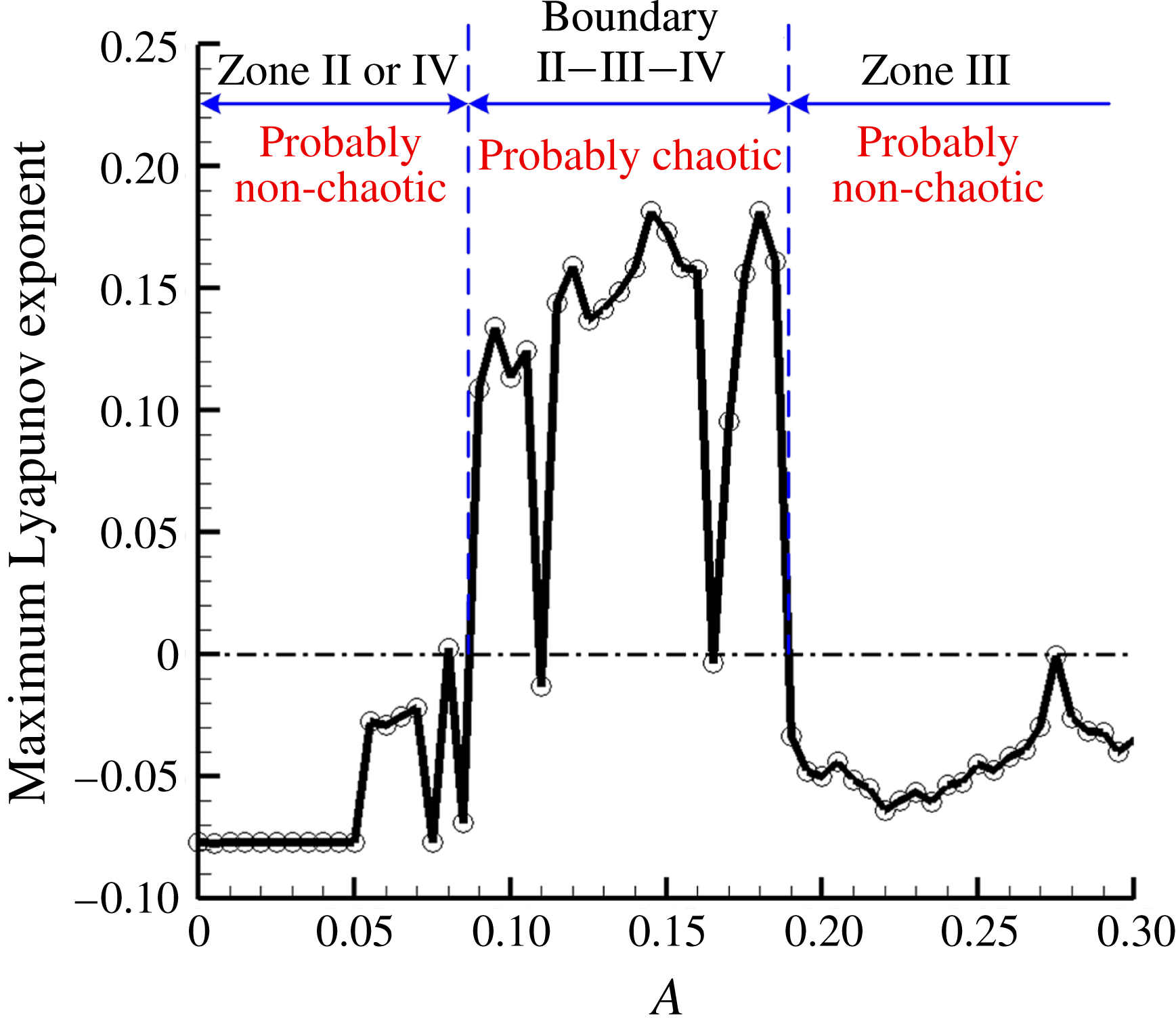
Maximum Lyapunov exponent versus
 $A$
.

In (2.5), the parameters
 $\unicode[STIX]{x1D714}_{0}$
,
 $r_{0}$
,
 $\unicode[STIX]{x1D719}_{0}$
and
 $K_{d}$
are selected as 1.1, 1, 0 and 0.154, respectively. The value of
 $\unicode[STIX]{x1D714}_{0}$
is selected as 1.1 to normalize the Duffing equation (Kovacic & Brennan Reference Kovacic and Brennan2011) where
 $a=1$
. The selection of
 $r_{0}$
and
 $\unicode[STIX]{x1D719}_{0}$
is merely for the sake of simplicity. The value of
 $K_{d}$
is dependent on the dissipation in the actual flow (or Reynolds number). It is selected by referring to the work by Lima & Pettini (Reference Lima and Pettini1990). As mentioned before,
 $A$
is related to the amplitude of the K–H unstable wave received by the fluid particle, and in fact, the value of
 $A$
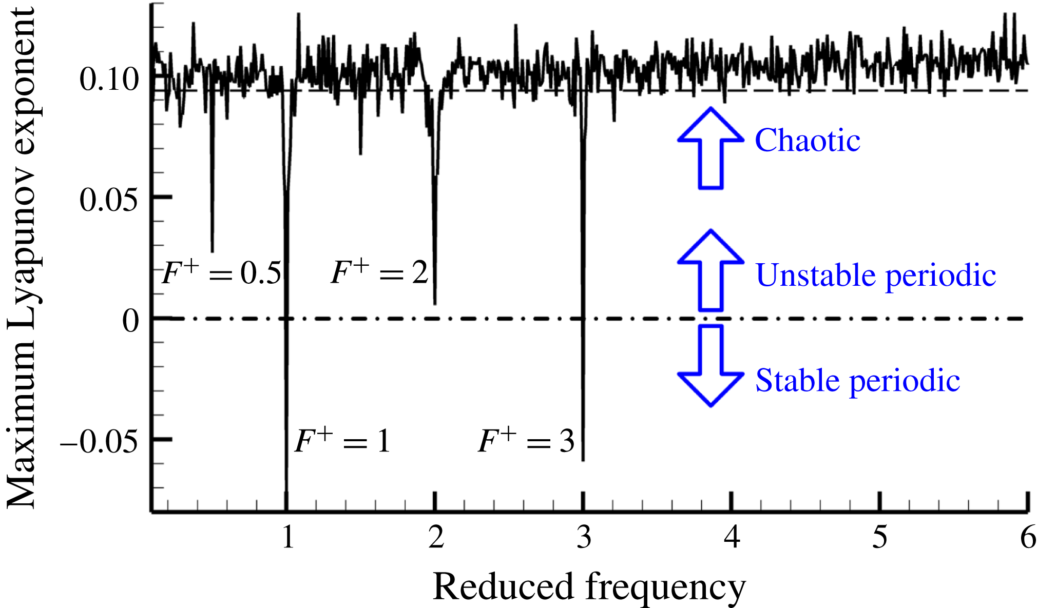
generally decides which zones the flow particle tends to fall into. Figure 4 shows the relationship between the maximum Lyapunov exponent and
 $A$
, when the other parameters are identified as above. Apart from some small windows, when
 $A<0.085$
, the fluid particle tends to stay in either Zone II or IV; when
 $0.085<A<0.19$
, the fluid particle tends to jump between Zones II, III, and IV, with its motion being chaotic; and when
 $0.19<A$
, the fluid particle tends to stay in Zone III. Chaos means the flow particle jumps back and forth between Zones II, III, and IV, in a seemingly random way, indicating that it is in the vicinity of the unstable Boundary II–III–IV, which is exactly what the model aimed to describe, as discussed before. Thus, in this paper,
 $A$
is selected as 0.088, just large enough to create chaos. Finally, the SCDM model without external excitation used here is
 $$\begin{eqnarray}\frac{\text{d}^{2}y}{\text{d}t^{2}}=y-4y^{3}-0.154\frac{\text{d}y}{\text{d}t}+0.088\sin (1.1t)\end{eqnarray}$$
 $y|_{t=-10}=0$
and
 $(\text{d}y/\text{d}t)|_{t=-10}=0$
are set as the initial conditions for (3.1). If the solutions of (3.1) are quasi-periodic or periodic, the initial condition and time-dependent term
 $f(t)$
together decide which zone (one of Zones II, III or IV) the fluid particle falls in. However, the influence of the initial condition then decays and vanishes quickly due to damping. Thus, the initial conditions are selected as resting at the unstable stationary point between Zones II and IV, and only the time-dependent term
 $f(t)$
decides which zone the fluid particle falls in. However, if the solution of (3.1) is chaotic, the long-term response is unpredictable and with intrinsic randomness, giving a definite initial condition (Butterfly effect), so the long-term chaotic characteristic of its solution is independent of the initial conditions as long as appropriate (Kovacic & Brennan Reference Kovacic and Brennan2011). It is notable that the time duration presented in figures 5 and 10 is long enough (10 s) after the start time
 $(t=-10~\text{s})$
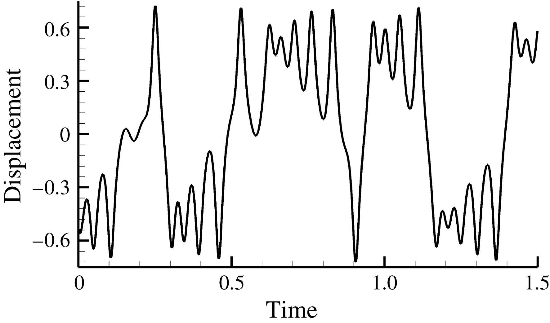
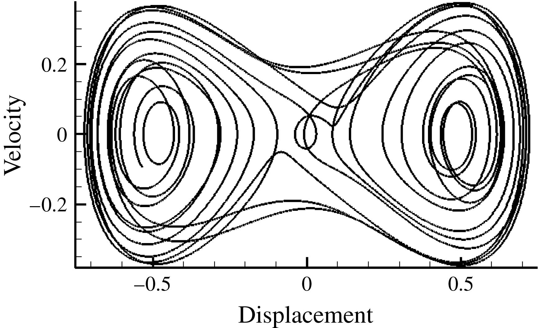
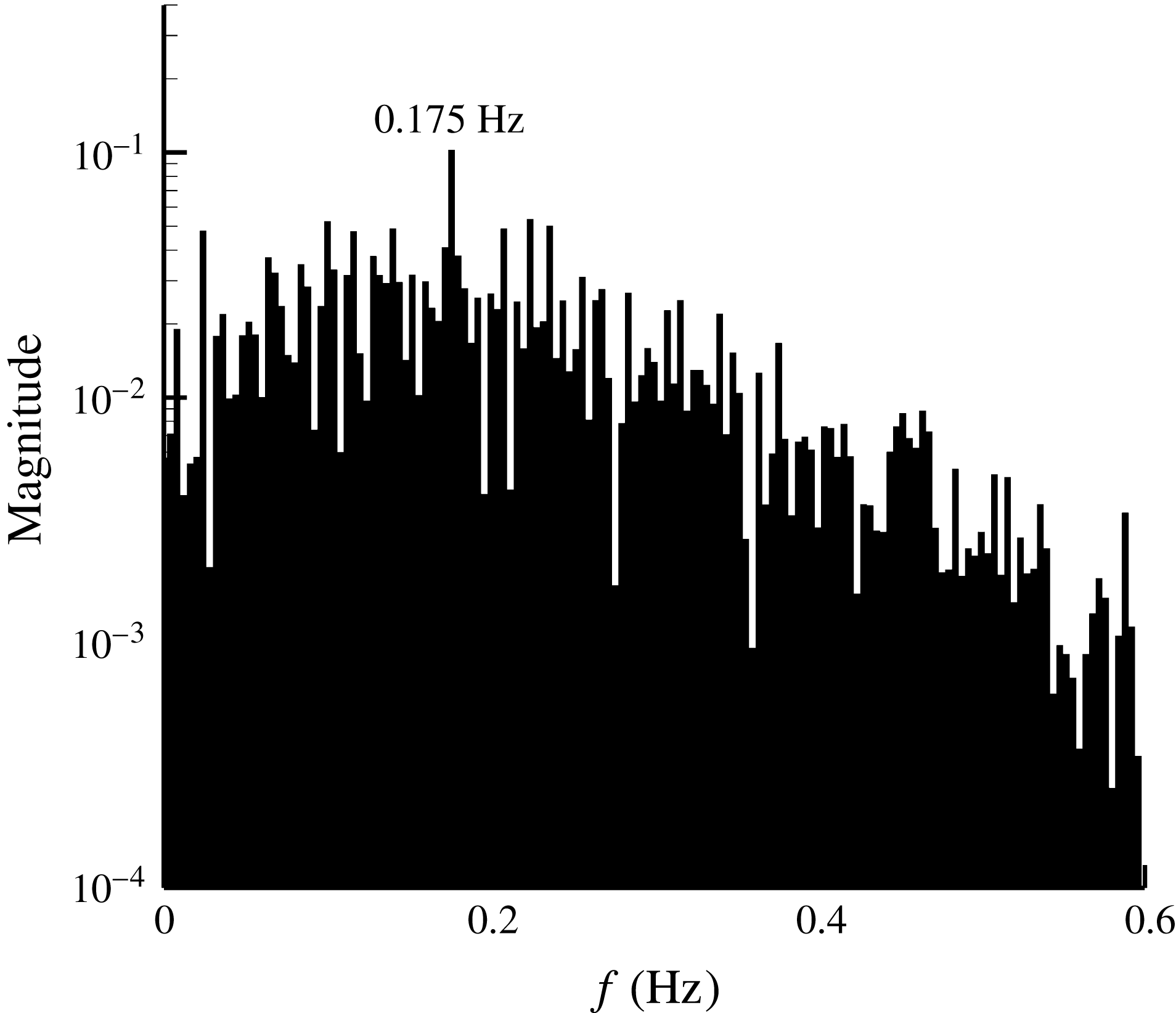
, which guarantees that the impact of the initial condition almost completely disappears. The corresponding time–displacement diagram and velocity–displacement phase diagram of (3.1) are shown in figures 5 and 6. With these two figures, it is seen that the fluid particle fluctuates from one attractor to another, and has difficulty in forecasting the tendency of its motion. This kind of phenomenon can be interpreted as that the flow particle, affected by the excitation of K–H unstable waves, may randomly fall into one of Zones II, III or IV, and no stable periodic fluctuation can be found. However, according to the frequency spectrum shown in figure 7, the dominant frequency of this fluctuation is approximately 0.175 Hz, which is equal to the frequency of the K–H term (
 $\unicode[STIX]{x1D714}_{0}=1.1$
) of the SCDM model as shown in (3.1), coexisting with the other clutter because of the chaotic motion. It means that K–H wave is still the main periodic behaviour in this seemingly random chaotic phenomenon. Generally, it can be concluded that the behaviours of the SCDM model correspond with the main characteristics (Lorenz Reference Lorenz1963) of typical chaotic dynamic systems, which are shear layers or separated flows.
Time-domain curve of displacement without excitation.

Velocity–displacement phase diagram without excitation.

Frequency spectrum of the velocity without excitation.

To analyse the unsteady control mechanism effectively, some of the overall performance parameters should be introduced to evaluate the control effects in different control states. The maximum Lyapunov exponent is then used to identify the degree of order of the coherent structure under different controls. More information about the maximum Lyapunov exponent and its calculation methods can be found in Benettin et al. (Reference Benettin, Galgani, Giorgilli and Strelcyn1980). Based on the calculation method, when the integral time
 $\unicode[STIX]{x1D70F}=0.01$
and the integral number
 $n=1000$
, the maximum Lyapunov exponent is approximately 0.093, which is larger than zero, implying that the dynamic system is in a chaotic condition without the flow control.
4 Analysis of the behaviour of the SCDM model with external excitation and the ordering mechanism
The unsteady flow control method is based on wave–vortex interactions or other mechanisms. According to the wave–vortex interaction analysis, the key problem is the coupling phenomenon between the original unsteady wave and the injected waves of the forced excitation (Zheng et al.
Reference Zheng, Zhou and Zhou2005). Also, to influence the original vortex, the injected waves should interact with the original unsteady wave, which is represented as a K–H wave in the SCDM model. Thus, the original K–H wave has been changed by the injection of the unsteady external excitation. In this paper, the amplitude of the K–H wave
 $A$
in (2.5) is altered to represent this change.
With the acoustic–vortex interaction results of the plate boundary layer, along with the injection of the acoustic wave, the original vorticity distribution of the boundary layer has been perturbed (Saric, Reed & Kerschen Reference Saric, Reed and Kerschen2002), and the disturbance is compensated by the Tollmien–Schlichting wave, of which the amplitude is proportional to the magnitude of the acoustic wave. Based on the previous results and the simultaneous consideration that the amplitude of the K–H wave is modified periodically by unsteady external excitation, an unsteady control term is then added to the source term by changing the coefficient
 $A$
of the SCDM model. In particular, the source term
 $A\cos (\unicode[STIX]{x1D714}_{0}t+\unicode[STIX]{x1D719}_{0})$
is modified to
 $(A+\unicode[STIX]{x1D702}\cos (\unicode[STIX]{x1D714}t+\unicode[STIX]{x1D719}))\cos (\unicode[STIX]{x1D714}_{0}t+\unicode[STIX]{x1D719}_{0})$
similar to amplitude modulation (AM), where
 $\unicode[STIX]{x1D702}$
represents the intensity of periodic external excitation,
 $\unicode[STIX]{x1D714}$
is its frequency and
 $\unicode[STIX]{x1D719}$
is its excitation phase. Based on equation (2.5), the SCDM model with external excitation is obtained as
 $$\begin{eqnarray}\frac{\text{d}^{2}y}{\text{d}t^{2}}=ay+cy^{3}-K_{d}\frac{\text{d}y}{\text{d}t}+(A+\unicode[STIX]{x1D702}\cos (\unicode[STIX]{x1D714}t+\unicode[STIX]{x1D719}))\cos (\unicode[STIX]{x1D714}_{0}t+\unicode[STIX]{x1D719}_{0}).\end{eqnarray}$$
Maximum Lyapunov exponent versus reduced frequency (SCDM results).

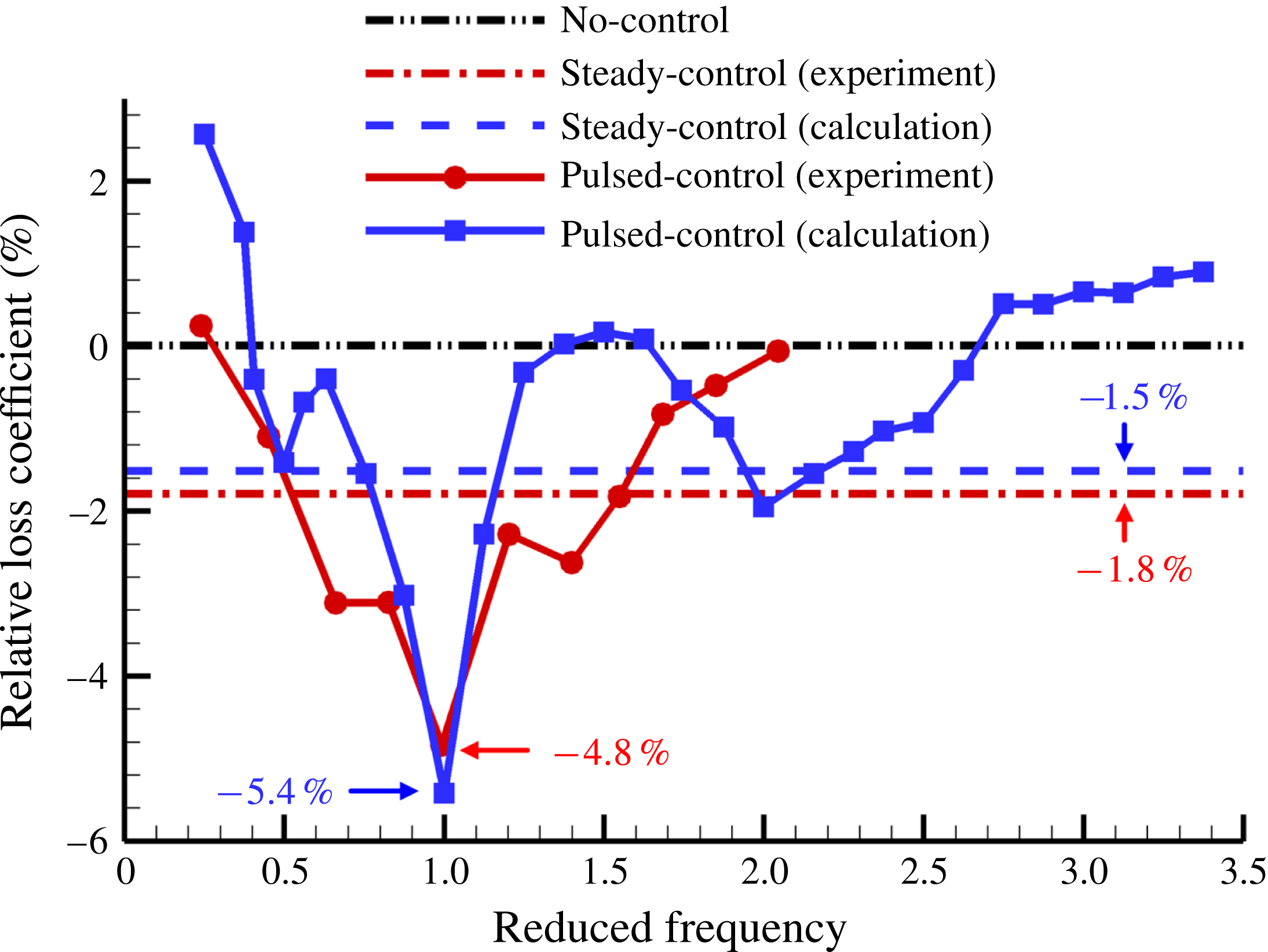
Relative loss coefficient versus reduced frequency (numerical and experimental results).

To verify validity of the SCDM model, the influence of the excitation frequency has been initially investigated. The maximum Lyapunov exponent for different reduced frequencies (
 $F+=\unicode[STIX]{x1D714}/\unicode[STIX]{x1D714}_{0}$
) is shown in figure 8 with the intensity
 $\unicode[STIX]{x1D702}=0.01$
and phase
 $\unicode[STIX]{x1D719}=0^{\circ }$
, where the reduced frequency is defined as the frequency of the external excitation divided by the main system frequency (
 ${\approx}0.175$
Hz in no control state). In figure 8, the maximum Lyapunov exponent is found to be reduced in half-octave, one-octave, two-octave and three-octave states. It means that when the frequency of external excitation is in those states, the fluctuation characteristics will be less chaotic, even to stable or unstable periodic states, from the chaotic state. When the frequency of excitation is equal to the main system frequency, the control effect is most remarkable.
The corresponding numerical and experimental results of a series of flow separations in the curved diffuser with different excitation frequencies are obtained by our study and the relative losses of the mechanical energy are shown in figure 9. The detailed information of the separated flows will be introduced in the following part (§ 6) and recent work (Zhu et al. Reference Zhu, Huang, Fu, Fu and Yu2013). The relative loss coefficient decreases obviously in half-octave, one-octave, and two-octave states in the numerical results shown in figure 9, while the experimental results displayed almost the same regularity, as shown in the same figure. Both numerical and experimental results verify the validity of the SCDM model. However, the experimental results only decrease obviously in the one-octave state, maybe because of complex vortical structures due to the 3D effect, although there is an attempt to avoid this. In both the numerical and experimental results, the unsteady control effects are more obvious when the frequency of excitation is equal to the dominant frequency of the flow field – as also reported in other studies (Greenblatt & Wygnanski Reference Greenblatt and Wygnanski2000; Zheng et al. Reference Zheng, Zhou and Zhou2005) – mutually confirming the outcomes of this study and other related research.
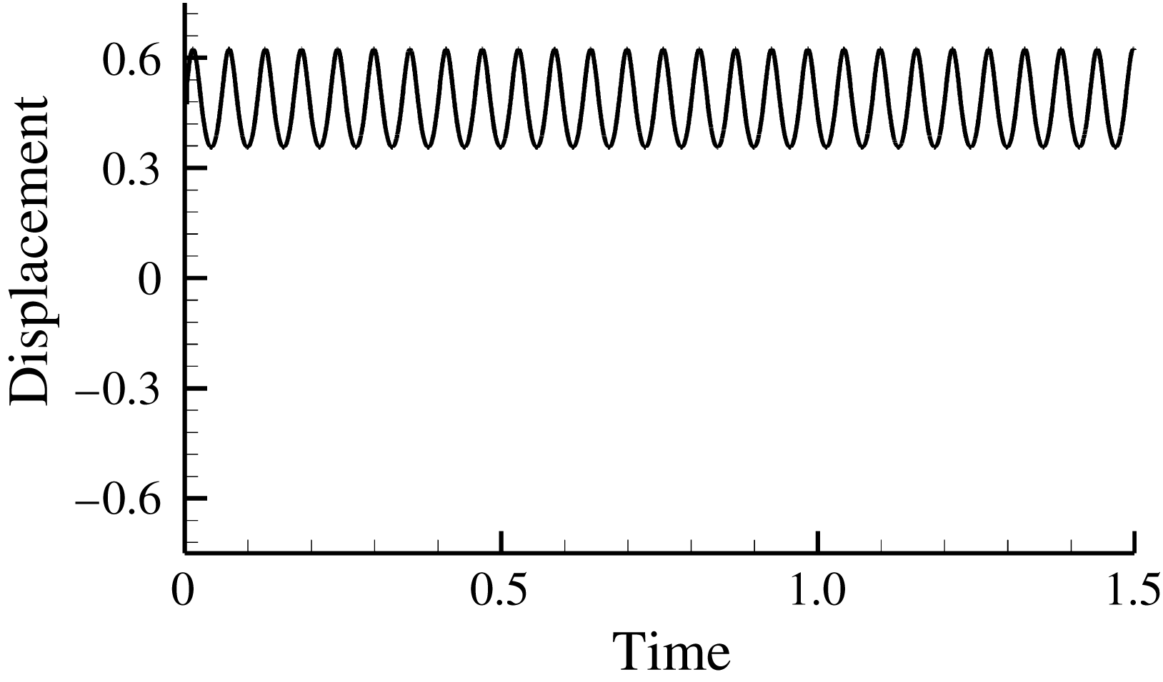
Time-domain curve of displacement with excitation (
 $F^{+}=1$
).

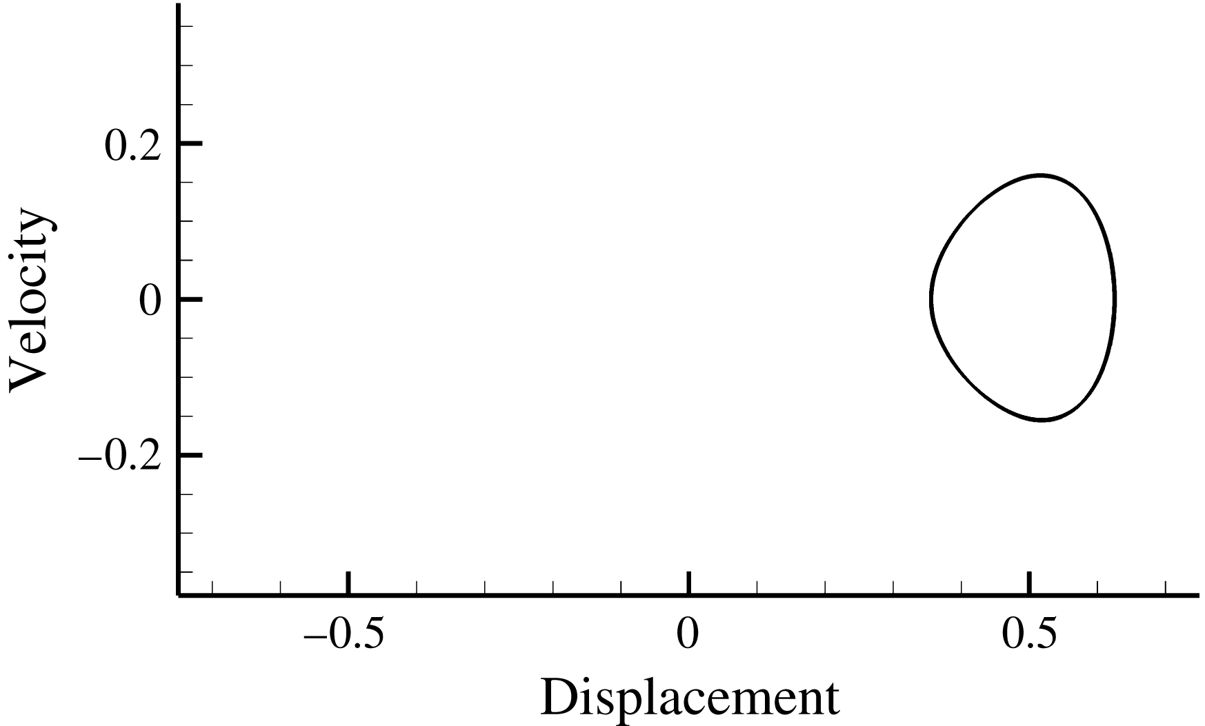
Velocity–displacement phase diagram with excitation (
 $F^{+}=1$
).

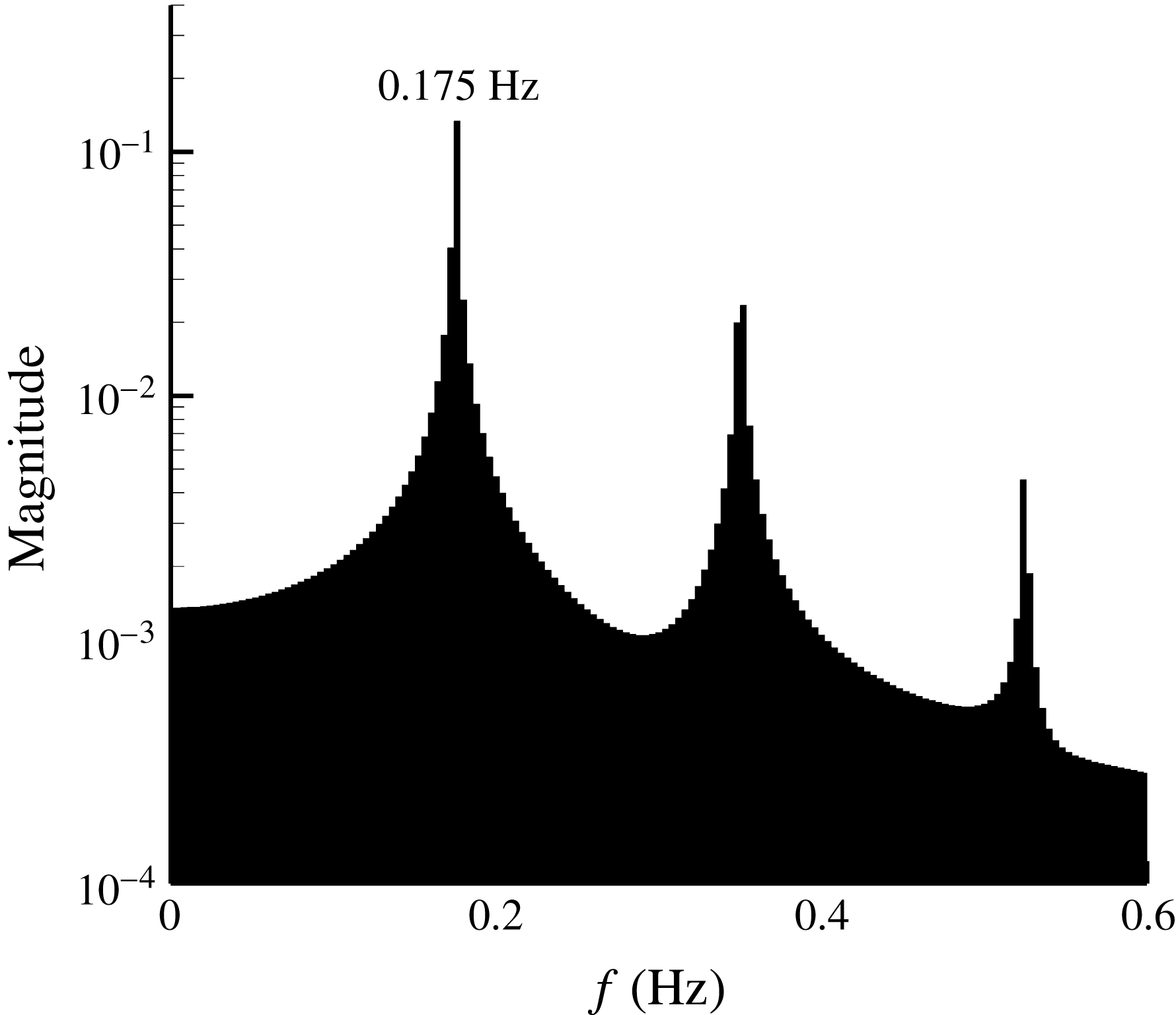
In addition, in identifying the mechanism of better control effect when the frequency of excitation is equal to the main system frequency, time-domain curves of the displacement and velocity–displacement phase diagram are seen in figures 10 and 11 when the reduced frequency is equal to 1. With the injection of periodic excitation, the fluid particle will fluctuate stably in Zone II (above the
 $x$
-axis), rather than jumping back and forth among Zones II, III, and IV. Its trajectory in the velocity–displacement phase diagram stabilizes around the right attractor, showing that the motion is entirely in order and periodic, with the signal corresponding to the maximum Lyapunov exponent, which is equal to
 $-0.078$
. Also, as shown in figure 12 and compared with figure 7, the frequency spectrum shows that the dominant frequency and its multiple frequencies are enhanced significantly, while clutter is suppressed because of the effective external excitation. They also indicate the motion is orderly and periodic. However, it should be noted that the stabilization of a certain fluid particle does not apply to all of the fluid particles in the flow field because the SCDM model is established based on the Lagrangian method and the fluid particle in the vicinity of Boundary II–III–IV. As cited earlier, different fluid particles in different zones may have their own set of parameters in the SCDM model, which will be partly discussed in § 5 in terms of synchronization.
Frequency spectrum of the velocity with excitation (
 $F^{+}=1$
).

In addition, from the SCDM model, it can be found that there is a minimum intensity for the external excitation (
 $\unicode[STIX]{x1D702}_{min}\approx 0.00063$
) to produce the control effect. It also means that there is a threshold intensity for unsteady flow control to function.
In general, the SCDM model outcomes correspond well with the known results by experimental and numerical studies carried out by our group and other researchers. It increases confidence in this model and encourages the exploration of further mechanisms in it, such as the self-synchronization mechanism.
5 Analysis of the mechanism of self-synchronization of unsteady flow separation with periodic excitation
Self-synchronization of unsteady separated flow with periodic excitation is a well-known and strange phenomenon in recent flow control studies. Researchers have found that the main separated flow structure (e.g. shedding vortices) can always synchronize in any phase with the external periodic excitation. This phenomenon is entirely different from the linear interaction, where excitation and coherent flow are assumed to have linear dynamic behaviours. So self-synchronization has become a popular and strange behaviour of nonlinear systems. Although this event has been studied in non-chaotic nonlinear systems (Skop & Balasubramanian Reference Skop and Balasubramanian1995), the following analysis will attempt to explain it based on the newly proposed nonlinear SCDM model and from the perspective of chaos control.
In the context of this paper, the self-synchronization phenomenon can be interpreted by citing that the flow control effects are almost the same under different phases of the external periodic excitation. Self-synchronization is related to the motions of a large number of fluid particles (several oscillators). However, the SCDM model describes the motion of a single fluid particle because it uses the Lagrange method (single oscillator), so extending its adaptability for a greater number of fluid particles is needed. Considering different fluid particles, there will be differences in the phase
 $\unicode[STIX]{x1D719}_{0}$
of K–H waves versus the phase
 $\unicode[STIX]{x1D719}$
of the periodic excitation felt by them. Also, only the difference between
 $\unicode[STIX]{x1D719}_{0}$
and
 $\unicode[STIX]{x1D719}$
matters in the SCDM model. So it provides a simplified approach to describe the different fluid particles by fixing
 $\unicode[STIX]{x1D719}$
and altering
 $\unicode[STIX]{x1D719}_{0}$
. Such a method is used to analyse the self-synchronization phenomenon in the rest of this section.
Maximum Lyapunov exponent for different system phases.

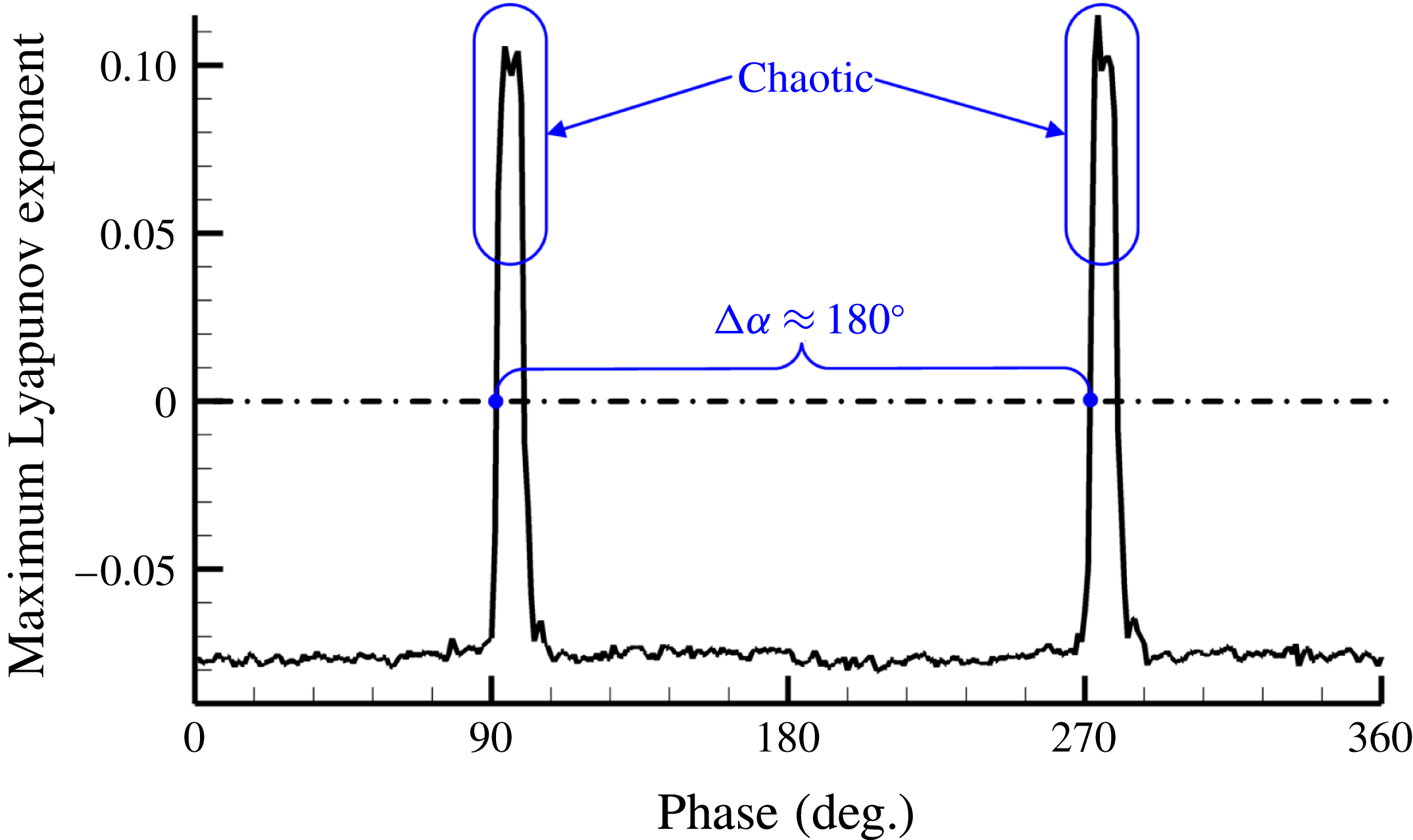
According to the results on the maximum Lyapunov exponent for different phases
 $\unicode[STIX]{x1D719}_{0}$
, as shown in figure 13, where
 $\unicode[STIX]{x1D714}=\unicode[STIX]{x1D714}_{0}=1.1$
,
 $\unicode[STIX]{x1D702}=0.01$
, and
 $\unicode[STIX]{x1D719}=0$
, the maximum Lyapunov exponent remains around
 $-0.078$
when
 $0^{\circ }\leqslant \unicode[STIX]{x1D719}_{0}<90^{\circ }$
,
 $105^{\circ }\leqslant \unicode[STIX]{x1D719}_{0}<270^{\circ }$
and
 $285^{\circ }\leqslant \unicode[STIX]{x1D719}_{0}<360^{\circ }$
. It implies that the system is in a stable periodic state under such conditions. However, when
 $90^{\circ }\leqslant \unicode[STIX]{x1D719}_{0}<105^{\circ }$
and
 $270^{\circ }\leqslant \unicode[STIX]{x1D719}_{0}<285^{\circ }$
, the maximum Lyapunov exponent increases obviously, similar to the state with no external excitation. It means that the external excitation cannot turn the fluctuation from the chaotic to the periodic state in these two relatively narrow ranges.
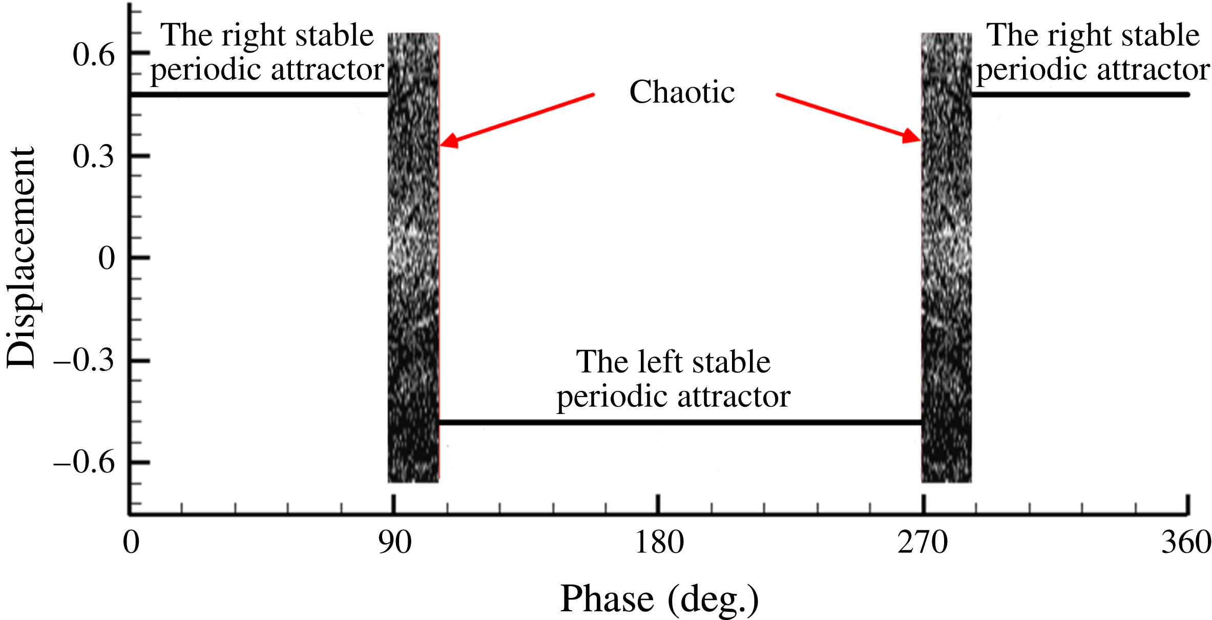
To analyse this phenomenon, the bifurcation diagram in relation to the different
 $\unicode[STIX]{x1D719}_{0}$
is shown in figure 14. When
 $0^{\circ }\leqslant \unicode[STIX]{x1D719}_{0}<90^{\circ }$
and
 $285^{\circ }\leqslant \unicode[STIX]{x1D719}_{0}<360^{\circ }$
, the oscillation is around the right stable periodic attractor, while when
 $105^{\circ }\leqslant \unicode[STIX]{x1D719}_{0}<270^{\circ }$
, the oscillation is around the left stable periodic attractor. Otherwise, the oscillation is chaotic. These results show that the motions of the fluid particles have been controlled in a rather large phase range, stabilizing on one side of the shear layer (Zone II or IV), and the motions still stay in a chaotic status in a small phase range. Thus, the results show that the probability of effective control is larger than that of non-effective control when the parameters of the excitation are appropriate, even if the relative phase difference between the external excitation phase
 $\unicode[STIX]{x1D719}$
and the K–H wave phase
 $\unicode[STIX]{x1D719}_{0}$
is random.
Bifurcation diagram with respect to the parameter of the external excitation phase.

In this paper, the effective ratio
 $\unicode[STIX]{x1D709}$
is defined as the phase range of the maximum Lyapunov exponent, which is less than zero over the phase range possible (i.e.
 $360^{\circ }$
), for example, the effective ratio
 $\unicode[STIX]{x1D709}$
is approximately 0.92 in figure 13. The effective ratio
 $\unicode[STIX]{x1D709}$
is seen to have a close relation to the macroscopic control effect of external excitation, such as total pressure recovery in the actual flow. When the effective ratio
 $\unicode[STIX]{x1D709}$
is high, a greater number of flow particles tend to be periodic rather than chaotic in a probabilistic sense, as the phase
 $\unicode[STIX]{x1D719}_{0}$
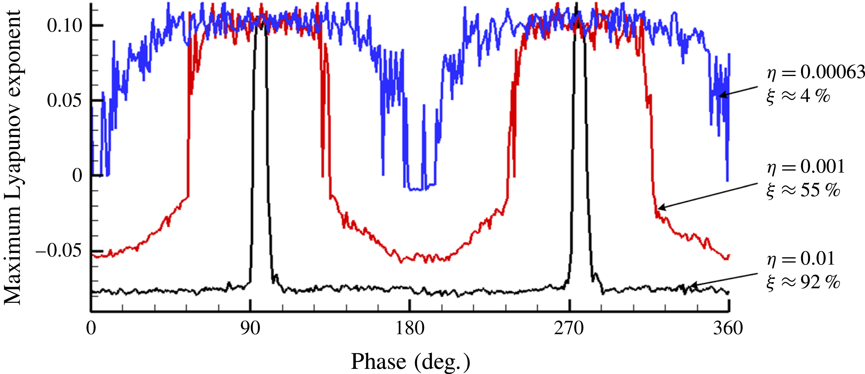
is random to observers. In figure 15, the effective ratio
 $\unicode[STIX]{x1D709}$
is also determined by the excitation intensity
 $\unicode[STIX]{x1D702}$
with the effective excitation frequency. As the excitation intensity
 $\unicode[STIX]{x1D702}$
increases from 0.00063 to 0.01, the effective ratio
 $\unicode[STIX]{x1D709}$
also increases, implying that the flow field is globally more ordered. But the effectiveness will not change obviously when the intensity
 $\unicode[STIX]{x1D702}$
exceeds 0.01. This is consistent with the existing experimental and numerical flow results (Zhu et al.
Reference Zhu, Huang, Fu, Fu and Yu2013).
The analysis above explains the mechanism of flow control for unsteady chaotic separated flows. In addition, the link among the microscopic SCDM model, the macroscopic control effect, and the self-synchronization phenomenon in actual flow are examined using chaos analysis. To summarize, the key of flow control of periodic external excitations is essentially relevant to changing the original chaotic flow into a relatively ordered flow.
Maximum Lyapunov exponent for the different phases in various intensity states.

6 Verification of the self-synchronization and flow field ordering mechanism in an actual separated flow with pulsed jet control in a curved diffuser
To validate self-synchronization and the flow field ordering mechanism as shown by the SCDM model, this investigation carried out the simulation of unsteady separated flow in a curved diffuser controlled by pulsed jets.
However, unsteady flow simulation generates a huge amount of information on the dynamic flow field, from which it is extremely hard to display the useful characteristics and laws of such coherent flow. The POD method is a helpful tool to overcome this difficulty. As an effective tool for data analysis and subsequent reduced-order modelling, POD has been applied to various engineering and scientific systems, including image processing (Holmes, Lumley & Berkooz Reference Holmes, Lumley and Berkooz1996), pattern recognition (Sirovich & Kirby Reference Sirovich and Kirby1987), and modelling of low-dimensional dynamics (Berkooz, Holmes & Lumley Reference Berkooz, Holmes and Lumley1993). In particular, POD is widely used to obtain approximate, low-dimensional descriptions of different turbulent fluid flows (Chatterjee Reference Chatterjee2000; Noack et al. Reference Noack, Afanasiev, Morzynski, Tadmor and Thiele2003; Tan, Damodaran & Willcox Reference Tan, Damodaran and Willcox2004; Akhtar, Nayfeh & Ribbens Reference Akhtar, Nayfeh and Ribbens2009b ). However, regarding reduced-order modelling, in some cases, the POD modes, while optimal based on the energy representation of a data set, may not be the best choice for reduced-order modelling, especially at higher Reynolds numbers (Kim & Bewley Reference Kim and Bewley2007). Thus, POD has been mainly used for data analysis (same function as the fast Fourier transfom (FFT)). For that purpose, it has already been used successfully in the analysis of flow fields with pulsed jet control by ourselves and others (Dano & Liburdy Reference Dano and Liburdy2006; Zhu et al. Reference Zhu, Huang, Fu, Fu and Yu2013). Based on POD and its analysis of spatiotemporal characteristics (Aubry, Holmes & Lumley Reference Aubry, Holmes and Lumley1988; Feng, Wang & Pan Reference Feng, Wang and Pan2011), it will be more effective to extract the coherent vortical structures and understand the mechanism of unsteady flow control. Initially, the POD method is briefly introduced.
A parameter in the time-dependent flow field
 $z(x,t)$
, where
 $x$
represents the space coordinate and
 $t$
represents the time coordinate, can be treated approximately as a finite summation in the form of separable variables:
 $$\begin{eqnarray}z(x,t)\approx \mathop{\sum }_{k=1}^{M}a_{k}(t)\unicode[STIX]{x1D711}_{k}(x).\end{eqnarray}$$
The time basis functions
 $a_{k}(t)$
and space basis functions
 $\unicode[STIX]{x1D711}_{k}(x)$
are not unique, although the POD method provides an algorithm employing singular value decomposition (SVD) to identify them and provide a physical meaning. From the mathematical point of view, the core idea of POD deals with calculating the best orthogonal basis functions or modes,
 $\{\unicode[STIX]{x1D711}_{k}(x),k=1,2,\ldots ,M\}$
, which ensure that the original function
 $z(x,t)$
can be precisely described with the fewest terms or modes, which means best fitting (Chatterjee Reference Chatterjee2000). In this paper, 200 snapshots (
 $M=200$
) are used for the POD analysis and the time interval of the two snapshots is
 $10^{-4}$
s. Considering the vortex shedding period is approximately
 $1/370$
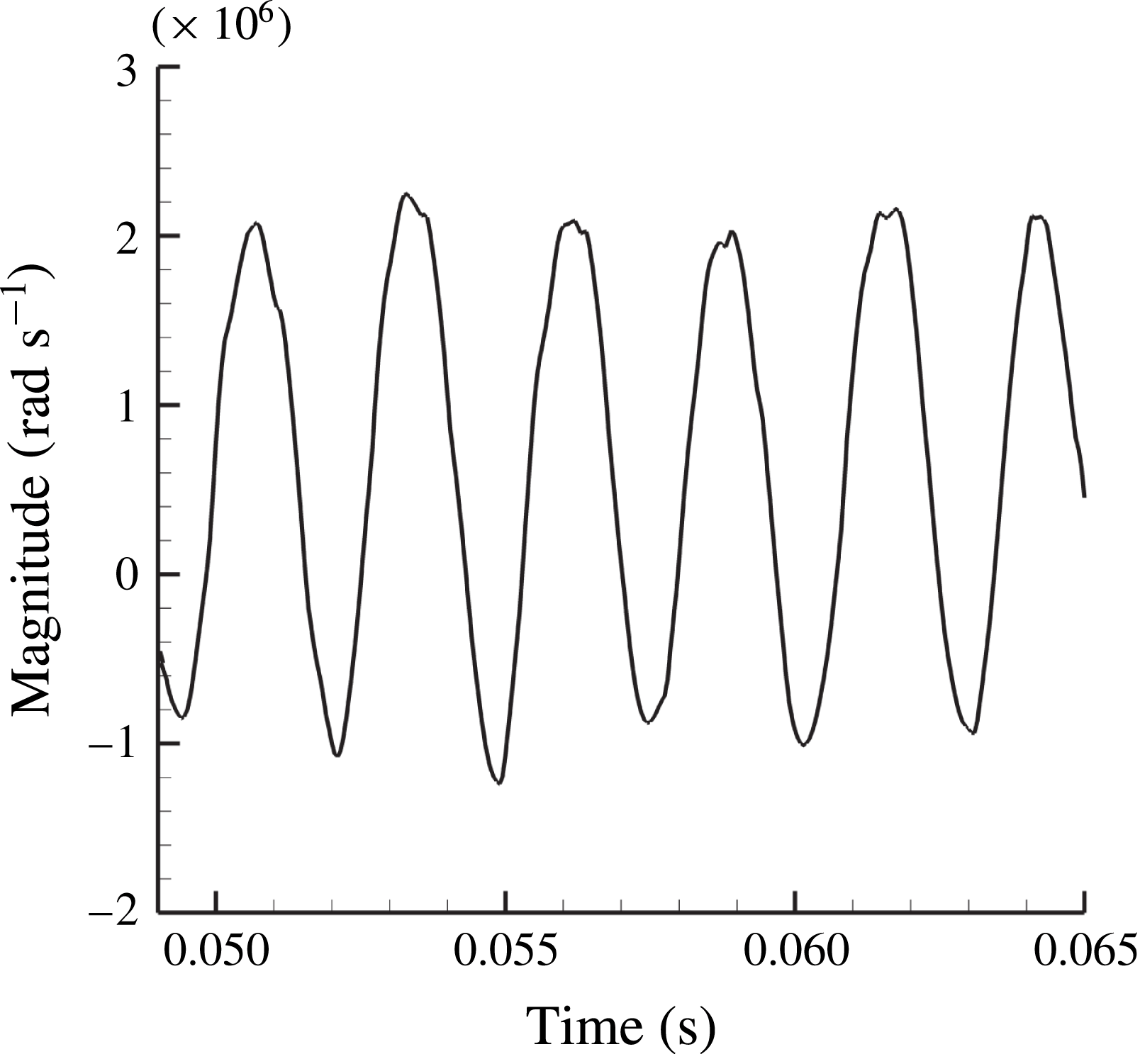
s, the number of oscillations during the 200 snapshots is approximately 7.4. The different POD modes represent the various flow structures in the flow field, and the magnitude of the mode (or modal value, singular values computed by SVD)
 $\unicode[STIX]{x1D706}_{i}$
presents the magnitude of the energy. Thus, the dominant modes have higher modal values, representing the large-scale or the main part of the flow structures, while others with smaller modal values reflect only the small-scale structures or trifling parts. Previous studies (Zhu et al.
Reference Zhu, Huang, Fu, Fu and Yu2013) have already shown that the first mode represents the structure of the time-averaged flow, both the second and third modes represent the structure of the separated vortices, and the other high-order modes represent the small-scale vortical structures. The coefficients
 $a_{k}(t)$
in (6.1) are also called modal coefficients, reflecting the instantaneous proportion of the modal flow structure to the origin flow field. The spectral information of a particular mode or flow structure can be reflected in them, so the modal coefficients of the lower order are focused on in the rest of this section. To summarize, the POD method can be used to decouple the spatial and temporal structures of the unsteady flow field and treat the actual unsteady flow field as the composition of various modes with different amplitudes for convenience of processing.
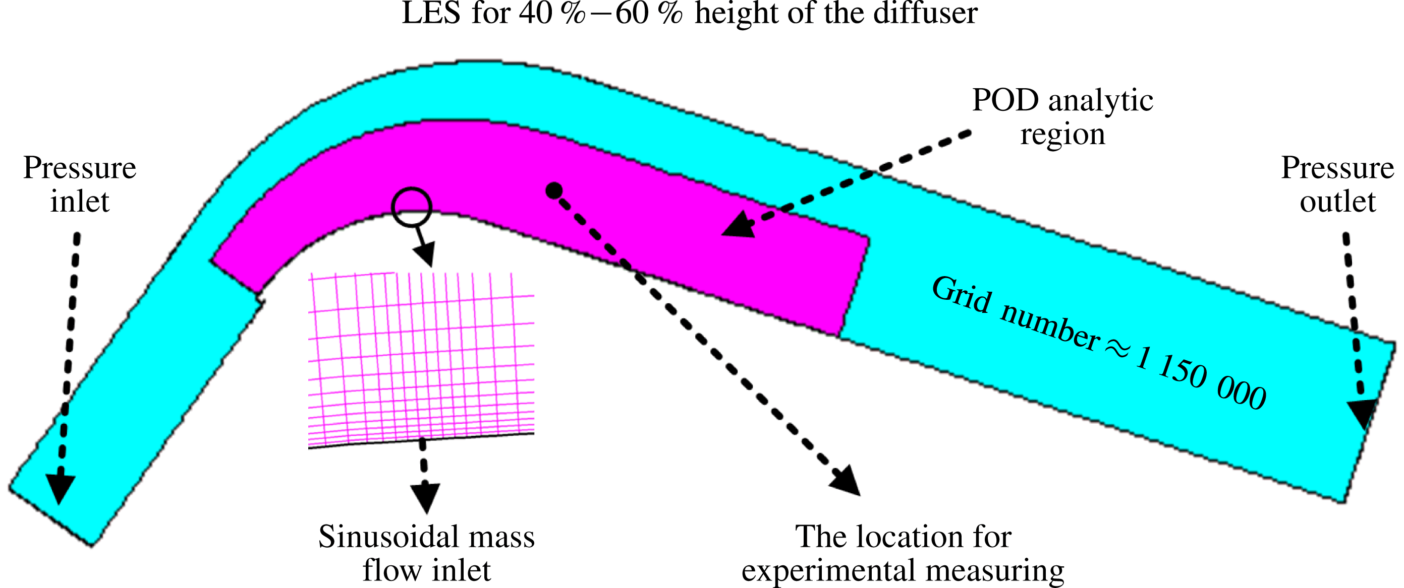
Computational domain with respect to the mid-section plane of the diffuser, other computational information and the location for experimental measuring.

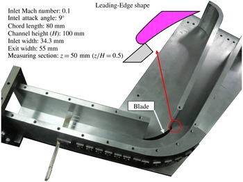
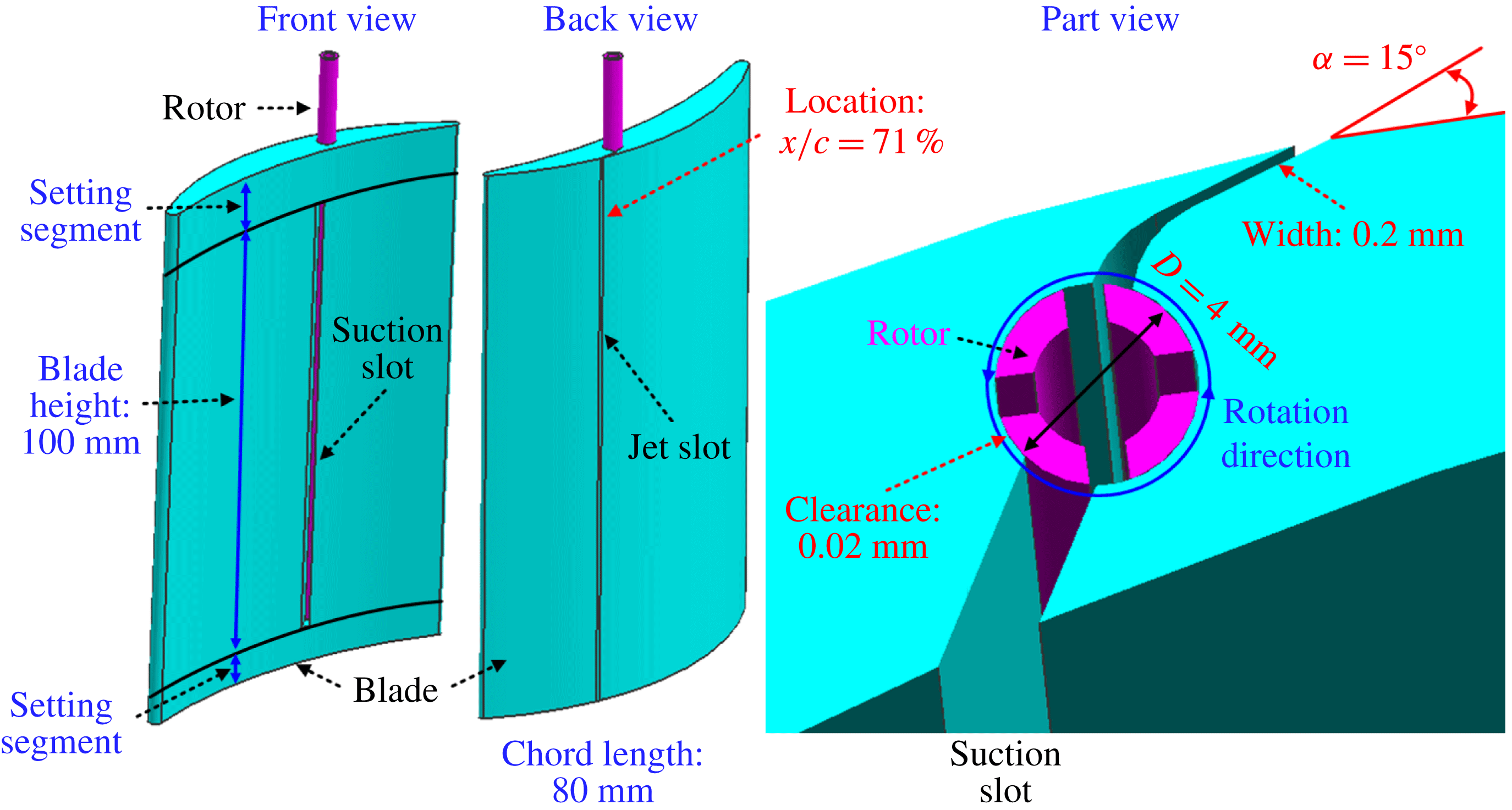
The model of diffuser for the numerical simulation and experiment is shown in figures 16 and 17. The diffuser consists of three parts, a blade using a double circular arc profile, a 34.3 mm long inlet, and a 55.5 mm long outlet. The blade chord length is selected as 80 mm (the Reynolds number defined by the length of blade chord is
 $1.81\times 10^{5}$
) and the height of the diffuser is 100 mm. For the experiment, the inlet Mach number is approximately 0.1 and the attack angle to the blade is approximately
 $9^{\circ }$
. The experiment has previously shown that the flow from 20 % to 80 % height of the diffuser could be regarded approximately as 2D flow (far from the secondary flow because of the influence of the shroud and hub). All measurements of this experiment were conducted at 50 % height of the diffuser to avoid the 3D flow effect, since 2D flow separation was focused on in this paper. The diagram of the pulsed jet device is shown in figure 17 (Zhu et al.
Reference Zhu, Huang, Fu, Fu and Yu2013). The width of the jet slot is 0.2 mm, the direction of blowing to the mainstream is
 $15^{\circ }$
, and the location of the jet is at approximately 71 % chord length. Also, the mean and oscillatory momentum coefficients (definition, see Greenblatt & Wygnanski Reference Greenblatt and Wygnanski2000) of this pulsed jet are 0.3 % and 0.15 %, respectively.
Photo of experimental devices.

Data related to the numerical simulation are presented in figure 16. LES is used in relation to a simplified model of the diffuser (limited by computing resources), with the influence of the small vortices added by the Smagorinsky–Lilly subgrid model. Compared to the experimental model, only 20 % of its height (20 mm high) around the mid-section plane was used for the simulation. The total number of the grids is approximately 1 150 000, with a refined mesh near walls, leading edges, and trailing edges (satisfying the needs of LES that
 $y^{+}\approx 1$
near walls). The boundary conditions of the inlet and exit are set to keep the inlet Mach number equal to 0.1. Periodic conditions are set for the upper and lower boundaries to avoid secondary flow as far as possible, and the periodic pulsed jet is set by a given sinusoidal time-dependent mass flow with a certain jet intensity. Dual-time stepping was used to realize the time-marching computation, and the physical time step is
 $10^{-5}~\text{s}$
. When the flow field turns into a periodic or quasi-periodic state, the computation is considered as converged. For the numerical simulation, more detailed information can be found in Feng et al. (Reference Feng, Wang and Pan2011).
Initially, numerical simulations of different excitation frequencies have been conducted. The pulsed jet is injected from a slot located on the lower surface (see figures 16 and 18). The results have already been shown in figure 9, corresponding with the works by Aubry et al. (Reference Aubry, Holmes and Lumley1988). With the pulsed jet of reduced frequency,
 $F^{+}=1$
, the energy loss is smaller than the other cases.
Then, flow fields with different excitation phases (
 $\unicode[STIX]{x1D719}=0^{\circ },120^{\circ },240^{\circ }$
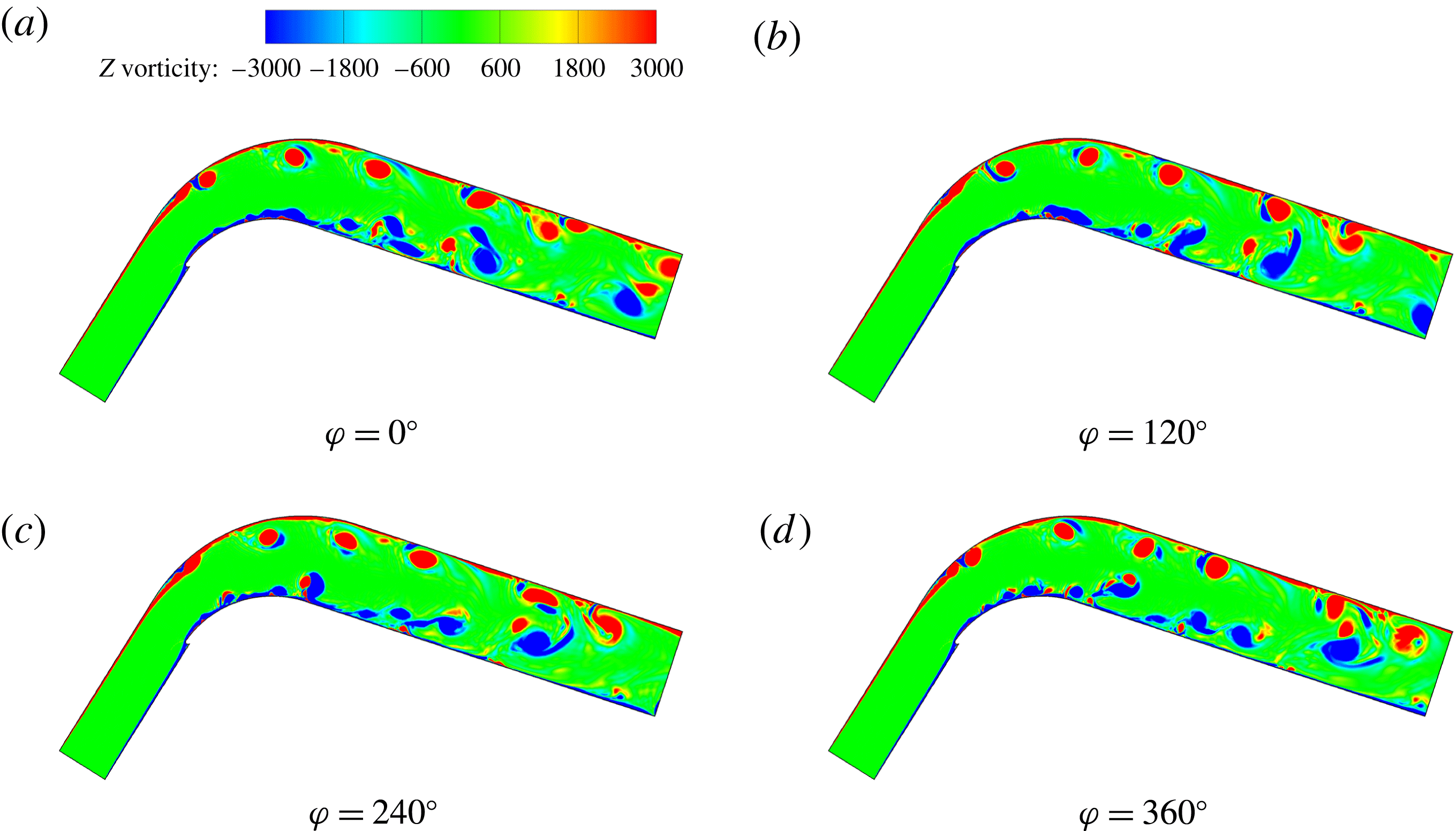
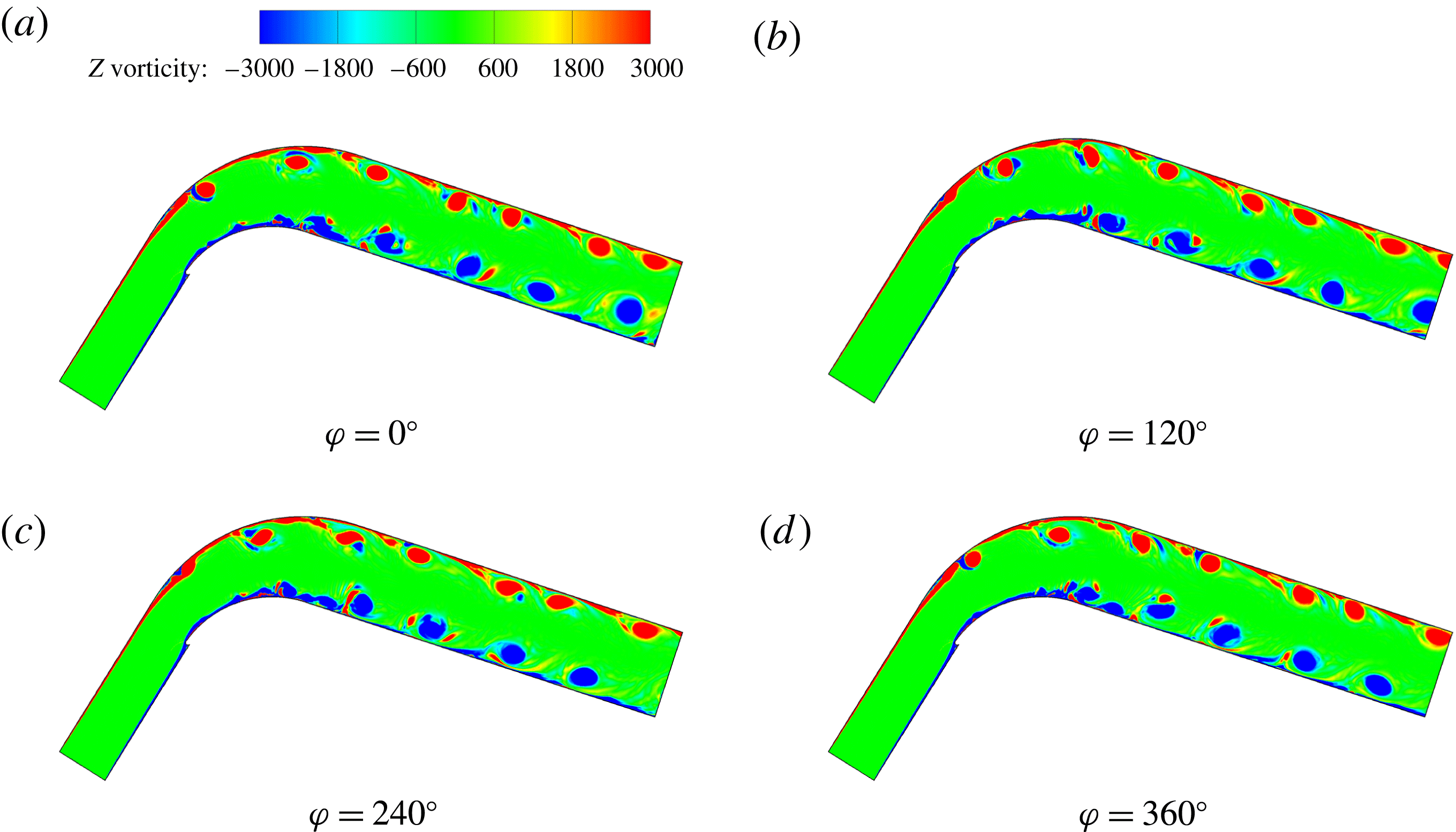
) were simulated when the reduced frequency equals 1. The results show that the overall control effects are similar. Such numerical simulations have verified the self-synchronization again. Typical instantaneous vorticity contours of the diffuser flow field without control and with fine control of
 $F^{+}=1$
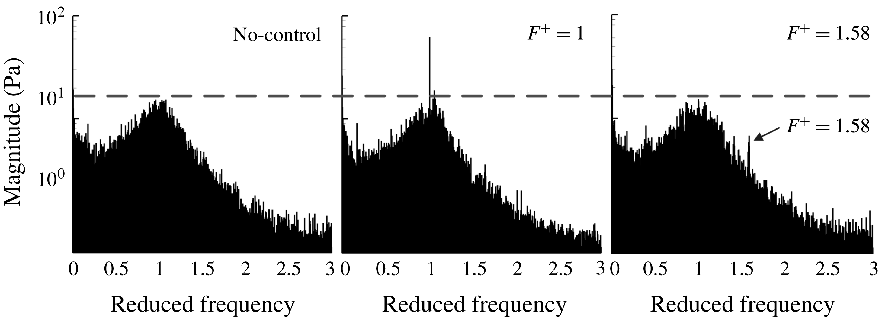
are shown in figures 19 and 20 for comparison. As observed, the structure of the controlled flow (figure 20) is relatively ordered compared with the original (figure 19), especially near the lower surface. It seems that the shedding vortices travel downstream independently, with less interaction with each other. So the flow mixing is decreased, contributing to reduced energy loss. Although the detailed flow fields were not measured because of the limitations of the experimental equipment, the measurements of the dynamic pressure at a certain number of fixed positions also support what was found in the numerical simulation. The FFT frequency spectra of the dynamic pressure at a typical location, as shown in figure 16, are illustrated in figure 21, corresponding to the three cases: without control, with valid control, and with invalid control, respectively. The repeated experiments, in which excitation phases are not intentionally aimed at a certain value and regarded as a random quantity, do not change the spectrum. Thus, self-synchronization also occurs in the experiments for which the control effect will not vary with the random excitation phases. Also, in figure 21, the valid control with
 $F^{+}=1$
makes the original dominant frequency in the case without control more remarkable (the same phenomenon also occurs in the SCDM model, see figures 7 and 12), corresponding to the improvement of the orderliness found in the numerical simulation in figure 20, whereas the invalid control with
 $F^{+}=1.58$
seems to have almost no effect on the improvement of the orderliness, resulting in only a small effect, as shown in figure 9 (the reason for choosing
 $F^{+}=1.58$
to discuss here is that it is a typical state where the control is not so effective in the experiment, as shown in figure 9).
Diagram of the pulsed jet device.

Instantaneous vorticity contour of diffuser flow field without control.

Instantaneous vorticity contour of diffuser flow field with effective control (
 $F^{+}=1$
).

Experimental frequency spectrum of dynamic pressure of a typical measuring point without control, with valid control, and with invalid control.

 $U$
–
 $V$
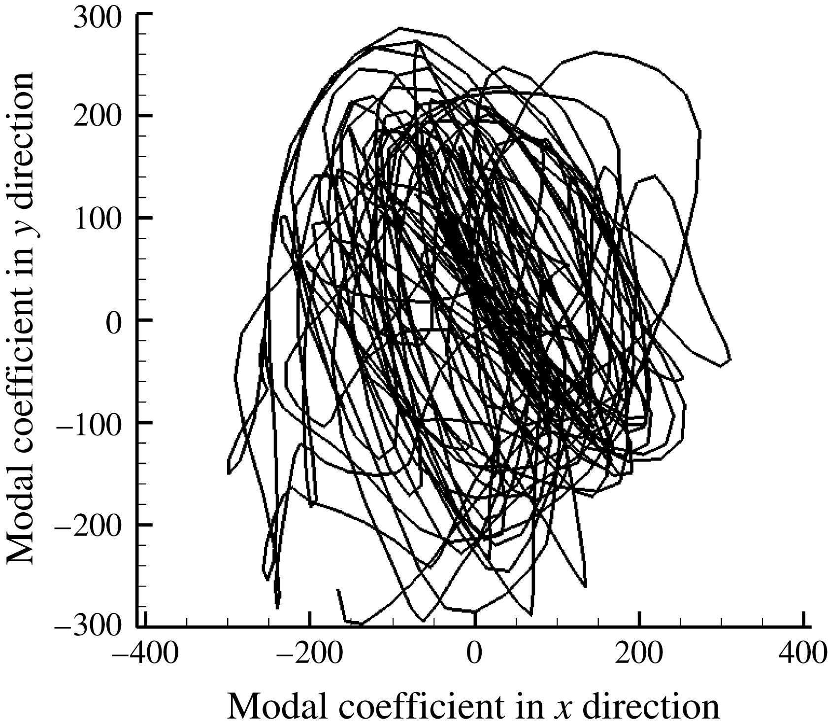
phase diagram (without control).

 $U$
–
 $V$
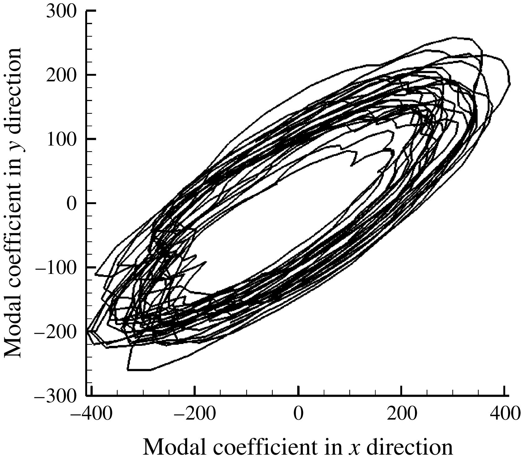
phase diagram (with
 $F^{+}=1$
control).

In addition, the
 $U$
–
 $V$
phase diagrams of the second POD mode for flows without control and with
 $F^{+}=1$
control are displayed in figures 22 and 23, which represent the main characteristics of the separation vortices. Here
 $U$
represents the modal coefficient of velocity in the
 $x$
direction and
 $V$
represents the modal coefficient of velocity in the
 $y$
direction. Both
 $U$
and
 $V$
contain the information of amplitude and phase information of separation vortices. The second modal coefficient indicates the instantaneous proportion of the dominant vortical structure to the whole flow field, representing the temporal fluctuation of the separation vortices in the
 $x$
or
 $y$
direction (Aubry et al.
Reference Aubry, Holmes and Lumley1988). The POD results (figures 22 and 23) also show that the
 $U$
–
 $V$
phase trajectory of the controlled flow is more orderly than without control, and shedding vortices perform similarly in a very periodic way (figure 23), similar to the SCDM model results (figure 11). Moreover, figure 23 includes three trajectories of the controlled flows with different excitation phases (
 $\unicode[STIX]{x1D719}=0^{\circ },120^{\circ },240^{\circ }$
), and those trajectories are rather similar and overlapping each other. To be more intuitive, the second POD modal coefficient of the vorticity without control and with
 $F^{+}=1$
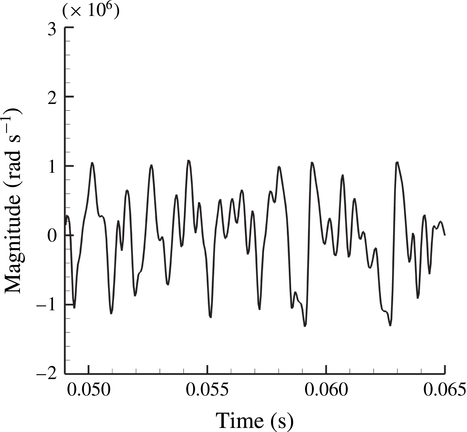
control is also displayed in figures 24 and 25. The one without control is cluttered (figure 24), similar to the results of the SCDM model (figure 5), while the one with effective control is orderly, approximating to a sine curve, with the same results as the SCDM model (figure 10).
The 2nd POD modal coefficient of vorticity without flow control.

The 2nd POD modal coefficient of vorticity with valid flow control (with
 $F^{+}=1$
control).

Briefly speaking, in § 2, a nonlinear dynamic model is established to describe motion of a fluid particle in the vicinity of Boundary II–III–IV in a separated flow. In § 3, it is found by analysis that its motion is chaotic without external excitation, just like in an actual separated flow. Then, the importance of the ordering mechanism is addressed in § 4. A study on the SCDM model of a single fluid particle indicates that effective periodic excitation control relies on the ordering mechanism, that external excitation of a particular frequency (such as
 $F^{+}=1$
) and appropriate intensity can change the motion of a fluid particle from chaos to order. Furthermore, in § 5, it is revealed that self-synchronization is a vital step to realize global order of a flow field. Analysis of the SCDM model based on a large number of fluid particles shows that most fluid particles tend to move periodically, affected by effective external excitation, making the flow field globally ordered. In addition, the control effect will not depend on the phase of excitation. Finally, in § 6, the preliminary explanation of periodic excitation control from the SCDM model is verified by an actual separated flow with pulsed jet control in a curved diffuser. Results discussed above in § 6 validate two major predictions of the SCDM model as: (1) the self-synchronization mechanism where the effect of periodic excitation control will depend only on the excitation frequency rather than its phase; and (2) the flow field ordering mechanism where appropriate periodic external excitation will make the global flow field more ordered.
7 Conclusions and summary
In exploring how periodic excitation controls separated flows effectively, a new nonlinear dynamic model has been established in this study. We not only carried out modelling and analysis based on the model but also used LES of unsteady separated flow in a diffuser controlled by pulsed jets. With the guidance of the model, the mechanism of flow field ordering and self-synchronization has been revealed, along with the LES of flows in the diffuser.
Below are the main points of the conclusion.
-
(1) Based on the 2D N–S equation, the Stuart vortex row, and the Lagrange method, a nonlinear simplified model (SCDM model) has been established, which is as follows:
(7.1)where
$$\begin{eqnarray}\frac{\text{d}^{2}y}{\text{d}t^{2}}=\unicode[STIX]{x1D700}\unicode[STIX]{x1D714}_{0}^{2}y-\frac{\unicode[STIX]{x1D700}\unicode[STIX]{x1D714}_{0}^{2}}{y_{s}^{2}}y^{3}-K_{d}\frac{\text{d}y}{\text{d}t}+A\sin (\unicode[STIX]{x1D714}_{0}t+\unicode[STIX]{x1D719}_{0}),\end{eqnarray}$$
$A\cos (\unicode[STIX]{x1D714}_{0}t+\unicode[STIX]{x1D719}_{0})$
is the source term representing the effect of K–H unstable wave,
$K_{d}(\text{d}y/\text{d}t)$
represents the dissipation effect, and
$\unicode[STIX]{x1D700}\unicode[STIX]{x1D714}_{0}^{2}y-(\unicode[STIX]{x1D700}\unicode[STIX]{x1D714}_{0}^{2}/y_{s}^{2})y^{3}$
acts as the complex interaction, including the nonlinear effect. The SCDM model analysis showed that it matched modelling requirements of coherent chaotic flows such as free shear and separated flows.
-
(2) Considering the periodic external excitation, an appropriate treatment of the external excitation has been added into the SCDM model. The maximum Lyapunov exponent has been introduced to evaluate the overall performance in the different control states. The results showed that the control effect was more obvious when the frequency of excitation is equal to the main system frequency. Also, the results of the SCDM model were validated by a comparison of the SCDM model and numerical and experimental results.
-
(3) Based on the SCDM model, the analysis presented an explanation of the mechanism of unsteady flow control for chaotic separated flows. The periodic excitation turns the original chaotic flow into a relatively ordered flow, and flow mixing is decreased, resulting in reduced energy loss. The mechanism was confirmed by the results of LES of coherent separated flow in a curved diffuser.
-
(4) The SCDM model analysis explained self-synchronization of unsteady separated flows and periodic excitations. When external excitation with an appropriate frequency and intensity is added, most of the fluid particles (with a different phase status) will be effectively controlled and the effect is independent of the phase of the external excitation. Also, when the intensity of excitation increases, the proportion of flow particles under control will increase and the flow field will be more ordered macroscopically.
-
(5) Under the guidance of this model, a typical flow control problem was examined by the experiment and numerical simulation. Several key points of the periodic excitation flow control were verified, such as the best reduced frequency of excitation
$F^{+}=1$
, the mechanism of effective periodic control (turning chaotic separated flow into ordered flow), and the self-synchronization phenomenon.




In summary, the SCDM model bridges the motions of microscopic fluid particles and the behaviours of macroscopic flows by a new approach, helping to analyse complex flow phenomena in an efficient and simplified way.
Acknowledgements
This work was supported by National Natural Science Foundation of China (Nos 51176072 and 51306089) and the National Basic Research Program of China (No. 2014CB239602).
Appendix A
Considering 2D incompressible N–S equation,
 $$\begin{eqnarray}\frac{\text{d}\boldsymbol{V}}{\text{d}t}=-\frac{1}{\unicode[STIX]{x1D70C}}\unicode[STIX]{x1D735}p+(\unicode[STIX]{x1D708}+\unicode[STIX]{x1D708}_{T})\unicode[STIX]{x1D6FB}^{2}\boldsymbol{V}.\end{eqnarray}$$
The actual flow field is rough because of the influence of turbulence, inhibiting further mathematical treatment such as Taylor expansion. Because isotropic small-scale turbulent eddies are not the main concern, in this equation they are filtered out and treated as a kind of subgrid-scale eddy viscosity (
 $\unicode[STIX]{x1D708}_{T}$
), learning from large eddy simulation. In Lagrangian coordinates,
 $x=x(\unicode[STIX]{x1D709},\unicode[STIX]{x1D702},t)$
and
 $y=y(\unicode[STIX]{x1D709},\unicode[STIX]{x1D702},t)$
, where
 $\unicode[STIX]{x1D709}$
,
 $\unicode[STIX]{x1D702}$
are Lagrange variables (conversely, they can also be described as
 $\unicode[STIX]{x1D709}=\unicode[STIX]{x1D709}(x,y,t)$
,
 $\unicode[STIX]{x1D702}=\unicode[STIX]{x1D702}(x,y,t)$
using Eulerian coordinates) used to distinguish the fluid particles. As cited earlier, only the
 $y$
-direction movement is considered, therefore, equation (A 1) can be restated as
 $$\begin{eqnarray}\frac{\unicode[STIX]{x2202}^{2}y(\unicode[STIX]{x1D709},\unicode[STIX]{x1D702},t)}{\unicode[STIX]{x2202}t^{2}}=-\frac{1}{\unicode[STIX]{x1D70C}}\frac{\unicode[STIX]{x2202}p(x,y,t)}{\unicode[STIX]{x2202}y}+(\unicode[STIX]{x1D708}+\unicode[STIX]{x1D708}_{T})\unicode[STIX]{x1D6FB}_{\unicode[STIX]{x1D709}\unicode[STIX]{x1D702}}^{2}\frac{\unicode[STIX]{x2202}y(\unicode[STIX]{x1D709},\unicode[STIX]{x1D702},t)}{\unicode[STIX]{x2202}t},\end{eqnarray}$$
where
 $$\begin{eqnarray}\displaystyle \unicode[STIX]{x1D6FB}_{\unicode[STIX]{x1D709}\unicode[STIX]{x1D702}}^{2} & = & \displaystyle (\unicode[STIX]{x1D709}_{x}^{2}+\unicode[STIX]{x1D709}_{y}^{2})\frac{\unicode[STIX]{x2202}^{2}}{\unicode[STIX]{x2202}\unicode[STIX]{x1D709}^{2}}+2(\unicode[STIX]{x1D709}_{x}\unicode[STIX]{x1D702}_{x}+\unicode[STIX]{x1D709}_{y}\unicode[STIX]{x1D702}_{y})\frac{\unicode[STIX]{x2202}^{2}}{\unicode[STIX]{x2202}\unicode[STIX]{x1D709}\unicode[STIX]{x2202}\unicode[STIX]{x1D702}}+(\unicode[STIX]{x1D702}_{x}^{2}+\unicode[STIX]{x1D702}_{y}^{2})\frac{\unicode[STIX]{x2202}^{2}}{\unicode[STIX]{x2202}\unicode[STIX]{x1D702}^{2}}\nonumber\\ \displaystyle & & \displaystyle +\,(\unicode[STIX]{x1D709}_{xx}+\unicode[STIX]{x1D709}_{yy})\frac{\unicode[STIX]{x2202}}{\unicode[STIX]{x2202}\unicode[STIX]{x1D709}}+(\unicode[STIX]{x1D702}_{xx}+\unicode[STIX]{x1D702}_{yy})\frac{\unicode[STIX]{x2202}}{\unicode[STIX]{x2202}\unicode[STIX]{x1D702}},\end{eqnarray}$$
and the subscripts mean partial derivatives here. For a particular fluid particle indicated as
 $\unicode[STIX]{x1D709}_{0}$
and
 $\unicode[STIX]{x1D702}_{0}$
,
 $$\begin{eqnarray}\frac{\text{d}^{2}y(\unicode[STIX]{x1D709}_{0},\unicode[STIX]{x1D702}_{0},t)}{\text{d}t^{2}}=\left.-\frac{1}{\unicode[STIX]{x1D70C}}\frac{\unicode[STIX]{x2202}p(x,y,t)}{\unicode[STIX]{x2202}y}\right|_{x=x(\unicode[STIX]{x1D709}_{0},\unicode[STIX]{x1D702}_{0},t),y=y(\unicode[STIX]{x1D709}_{0},\unicode[STIX]{x1D702}_{0},t)}+(\unicode[STIX]{x1D708}+\unicode[STIX]{x1D708}_{T})\unicode[STIX]{x1D6FB}_{\unicode[STIX]{x1D709}\unicode[STIX]{x1D702}}^{2}\left.\frac{\unicode[STIX]{x2202}y(\unicode[STIX]{x1D709},\unicode[STIX]{x1D702},t)}{\unicode[STIX]{x2202}t}\right|_{\unicode[STIX]{x1D709}=\unicode[STIX]{x1D709}_{0},\unicode[STIX]{x1D702}=\unicode[STIX]{x1D702}_{0}}.\end{eqnarray}$$
Initially, we can analyse the dissipation term, which is the second term on the right of equation (A 4). Fluid viscosity and small-scale vortex viscosity dissipate the mechanical energy of the fluid in general, but for the single particle
 $P$
it is hard to say whether the fluid viscosity serves as a driving force or resistance along the
 $y$
direction. However, viscosity often restrains growth in amplitude of K–H unstable waves and consumes kinetic energy in the
 $y$
-direction, making the fluid viscosity a damping force on average. For shear flow, the average velocity of the
 $y$
direction is zero while its transient velocity keeps oscillating. So the corresponding damping force should be proportional to the velocity difference between the particle
 $P$
and the adjacent zones. If we define the equivalent damping coefficient according to the time average as
 $$\begin{eqnarray}K_{d}=-(\unicode[STIX]{x1D708}+\unicode[STIX]{x1D708}_{T})\frac{\displaystyle \int _{0}^{T}\frac{\text{d}y(\unicode[STIX]{x1D709}_{0},\unicode[STIX]{x1D702}_{0},t)}{\text{d}t}\cdot \left.\left(\unicode[STIX]{x1D6FB}_{\unicode[STIX]{x1D709}\unicode[STIX]{x1D702}}^{2}\frac{\unicode[STIX]{x2202}y(\unicode[STIX]{x1D709},\unicode[STIX]{x1D702},t)}{\unicode[STIX]{x2202}t}\right)\right|_{\unicode[STIX]{x1D709}=\unicode[STIX]{x1D709}_{0},\unicode[STIX]{x1D702}=\unicode[STIX]{x1D702}_{0}}\,\text{d}t}{\displaystyle \int _{0}^{T}\left(\frac{\text{d}y(\unicode[STIX]{x1D709}_{0},\unicode[STIX]{x1D702}_{0},t)}{\text{d}t}\right)^{2}\,\text{d}t}.\end{eqnarray}$$
Then, the second term on right side of equation (A 4), can be replaced by the equivalent damping term,
 $K_{d}(\text{d}y(\unicode[STIX]{x1D709}_{0},\unicode[STIX]{x1D702}_{0},t)/\text{d}t)$
, which represents the equivalent time-averaged damping for kinetic energy. For simplicity,
 $x(t)$
is short for
 $x(\unicode[STIX]{x1D709}_{0},\unicode[STIX]{x1D702}_{0},t)$
and
 $y(t)$
is short for
 $y(\unicode[STIX]{x1D709}_{0},\unicode[STIX]{x1D702}_{0},t)$
. Equation (A 2) can be simplified as
 $$\begin{eqnarray}\left.\frac{\text{d}^{2}y(t)}{\text{d}t^{2}}=-\frac{1}{\unicode[STIX]{x1D70C}}\frac{\unicode[STIX]{x2202}p(x,y,t)}{\unicode[STIX]{x2202}y}\right|_{x=x(t),y=y(t)}-K_{d}\frac{\text{d}y(t)}{\text{d}t}.\end{eqnarray}$$
Then, we try to treat the pressure gradient term (neglecting viscous term temporarily). The interaction between the movement of the
 $x$
direction and the
 $y$
direction is neglected, by assuming that the
 $x$
-direction velocity of flow particle constantly equals the time-averaged velocity
 $\bar{u}$
. Regarding the unsteady pressure field
 $p(x,y,t)$
, it can be considered approximately in the view of averaged flow as
 $$\begin{eqnarray}p(x,y,t)\approx p(\bar{u}t,y,t)=p(y,t).\end{eqnarray}$$
In the neighbourhood of the path of the flow particle, there must be a location where
 $(\unicode[STIX]{x2202}p/\unicode[STIX]{x2202}y)=0$
; assuming the location is
 $y_{0}$
, about which the flow particle
 $P$
moves and a Taylor expansion of the pressure field,
 $p(y,t)$
, shows that
 $$\begin{eqnarray}\displaystyle p(y,t) & = & \displaystyle p(y_{0}(t),t)+\frac{\unicode[STIX]{x2202}p(y_{0}(t),t)}{\unicode[STIX]{x2202}y}(y-y_{0}(t))+\frac{1}{2}\frac{\unicode[STIX]{x2202}^{2}p(y_{0}(t),t)}{\unicode[STIX]{x2202}y^{2}}(y-y_{0}(t))^{2}\nonumber\\ \displaystyle & & \displaystyle +\,\frac{1}{3!}\frac{\unicode[STIX]{x2202}^{3}p(y_{0}(t),t)}{\unicode[STIX]{x2202}y^{3}}(y-y_{0}(t))^{3}+\frac{1}{4!}\frac{\unicode[STIX]{x2202}^{4}p(y_{0}(t),t)}{\unicode[STIX]{x2202}y^{4}}(y-y_{0}(t))^{4}+\cdots \,.\end{eqnarray}$$
Ignoring the high-order small quantity, the pressure gradient can be expressed approximately as follows:
 $$\begin{eqnarray}\frac{\unicode[STIX]{x2202}p(y,t)}{\unicode[STIX]{x2202}y}=-\unicode[STIX]{x1D70C}a(t)y-\unicode[STIX]{x1D70C}b(t)y^{2}-\unicode[STIX]{x1D70C}c(t)y^{3}-\unicode[STIX]{x1D70C}f(t).\end{eqnarray}$$
Among them,
 $a(t)$
,
 $b(t)$
,
 $c(t)$
and
 $f(t)$
are time-dependent functions. Then,
 $$\begin{eqnarray}\frac{\text{d}^{2}y}{\text{d}t^{2}}=a(t)y+b(t)y^{2}+c(t)y^{3}-K_{d}\frac{\text{d}y}{\text{d}t}+f(t).\end{eqnarray}$$
Appendix B
The analyses of the zones and the boundary in figure 2 are shown here.
Zone I, V:
The movement of flow particles is approximately regarded as uniform rectilinear motion (its
 $y$
-coordinate remains constant assuming
 $y_{s1}$
) in this zone. Thus,
 $$\begin{eqnarray}\displaystyle & \displaystyle y=y_{s1} & \displaystyle\end{eqnarray}$$
 $$\begin{eqnarray}\displaystyle & \displaystyle \frac{\text{d}^{2}y}{\text{d}t^{2}}=0=-\frac{1}{\unicode[STIX]{x1D70C}}\frac{\text{d}p}{\text{d}y} & \displaystyle\end{eqnarray}$$
 $$\begin{eqnarray}\displaystyle & \displaystyle p=C_{1}, & \displaystyle\end{eqnarray}$$
where
 $C_{1}$
is an arbitrary constant.
Zone II, IV:
The movement of flow particle is approximately regarded as a simple harmonic wave motion. In this zone, we assume its equilibrium position is
 $y_{s2}$
(
 $y_{s4}$
for Zone IV and take Zone II for example). The amplitude is
 $A_{2}$
(
 $A_{4}$
for zone IV), the angular frequency is
 $\unicode[STIX]{x1D714}_{2}$
(
 $\unicode[STIX]{x1D714}_{4}$
for Zone IV) and the phase angle is
 $\unicode[STIX]{x1D711}_{2}$
(
 $\unicode[STIX]{x1D711}_{4}$
for Zone IV). Thus,
 $$\begin{eqnarray}\displaystyle & \displaystyle y=y_{s2}+A_{2}\sin (\unicode[STIX]{x1D714}_{2}t+\unicode[STIX]{x1D719}_{2}) & \displaystyle\end{eqnarray}$$
 $$\begin{eqnarray}\displaystyle & \displaystyle \frac{\text{d}^{2}y}{\text{d}t^{2}}=-\unicode[STIX]{x1D714}_{2}^{2}(y-y_{s2})=-\frac{1}{\unicode[STIX]{x1D70C}}\frac{\text{d}p}{\text{d}y} & \displaystyle\end{eqnarray}$$
 $$\begin{eqnarray}\displaystyle & \displaystyle p=\frac{\unicode[STIX]{x1D70C}\unicode[STIX]{x1D714}_{2}^{2}}{2}(y-y_{s2})^{2}+C_{2}, & \displaystyle\end{eqnarray}$$
where
 $C_{2}$
(
 $C_{4}$
for Zone IV) is another arbitrary constant.
Zone III:
The movement of the flow particle is approximately regarded as uniform circular motion in this zone, of which the
 $y$
-direction movement is also a simple harmonic motion around the equilibrium point
 $y=0$
. It is assumed that the amplitude is
 $A_{3}$
, the angular frequency is
 $\unicode[STIX]{x1D714}_{3}$
and the phase angle is
 $\unicode[STIX]{x1D711}_{3}$
. Thus,
 $$\begin{eqnarray}\displaystyle & \displaystyle y=A_{3}\sin (\unicode[STIX]{x1D714}_{3}t+\unicode[STIX]{x1D719}_{3}) & \displaystyle\end{eqnarray}$$
 $$\begin{eqnarray}\displaystyle & \displaystyle \frac{\text{d}^{2}y}{\text{d}t^{2}}=-\unicode[STIX]{x1D714}_{3}^{2}y=-\frac{1}{\unicode[STIX]{x1D70C}}\frac{\text{d}p}{\text{d}y} & \displaystyle\end{eqnarray}$$
 $$\begin{eqnarray}\displaystyle & \displaystyle p=\frac{\unicode[STIX]{x1D70C}\unicode[STIX]{x1D714}_{3}^{2}}{2}y^{2}+C_{3}, & \displaystyle\end{eqnarray}$$
where
 $C_{3}$
is also an arbitrary constant.
Boundary II–III–IV:
From figure 2, it is known that Boundary II–III–IV is important topologically. The disturbance on each fluid particle in the vicinity of this boundary may bring it to Zone II, III or IV. Also, it is reasonable to consider that the pressure distribution of Boundary II–III–IV is in between that of Zones II, III, and IV. From figure 2, it is easy to find that nearby Boundary II–III–IV,
 $\unicode[STIX]{x1D714}_{2}=\unicode[STIX]{x1D714}_{4}=2\unicode[STIX]{x1D714}_{3}=2\unicode[STIX]{x1D714}_{0}$
(where
 $\unicode[STIX]{x1D714}_{0}$
is the characteristic frequency of the Stuart vortex received by the affected fluid particle) and
 $y_{s2}=-y_{s3}=y_{s}$
. Thus, from (B 6) and (B 9),
 $$\begin{eqnarray}\displaystyle & \displaystyle p=2\unicode[STIX]{x1D70C}\unicode[STIX]{x1D714}_{0}^{2}(y-y_{s})^{2}+C_{2}\quad y\in [0,2y_{s}] & \displaystyle\end{eqnarray}$$
 $$\begin{eqnarray}\displaystyle & \displaystyle p=2\unicode[STIX]{x1D70C}\unicode[STIX]{x1D714}_{0}^{2}(y+y_{s})^{2}+C_{4}\quad y\in [-2y_{s},0] & \displaystyle\end{eqnarray}$$
 $$\begin{eqnarray}\displaystyle & \displaystyle p=\frac{\unicode[STIX]{x1D70C}\unicode[STIX]{x1D714}_{0}^{2}}{2}y^{2}+C_{3}\quad y\in [-2y_{s},2y_{s}]. & \displaystyle\end{eqnarray}$$
In figure 2, it can be seen that when
 $y=\pm 2y_{s}$
, whether in Zone II, III or IV,
 $(\text{d}y/\text{d}t)=0$
and the pressure standing for potential energy on Boundary II–III–IV must be the same. Thus,
 $C_{2}=C_{3}=C_{4}$
, and we might also set them to be zero. However, when
 $y=0$
,
 $|\text{d}y/\text{d}t|$
equals zero in Zone II and IV, but reach its maximum in Zone III. Thus, the pressure of Boundary II–III–IV needs substantial modification at
 $y=0$
. The pressure distribution described by (B 10), (B 11), and (B 12) is shown in figure 26. As cited earlier, the pressure distribution of Boundary II–III–IV is in between that of Zones II, III, and IV, so it shares the extreme points, which are
 $y=\pm y_{s}$
and
 $y=0$
. Thus, the simplest form of the pressure distribution of this boundary can be described as
 $$\begin{eqnarray}\displaystyle p=-{\textstyle \frac{1}{2}}\unicode[STIX]{x1D70C}ay^{2}+{\textstyle \frac{1}{4}}\unicode[STIX]{x1D70C}cy^{4}+2(1-\unicode[STIX]{x1D700})\unicode[STIX]{x1D70C}\unicode[STIX]{x1D714}_{0}^{2}y_{s}^{2}\quad y\in [-2y_{s},2y_{s}]. & & \displaystyle\end{eqnarray}$$
The last term in equation (B 13) is a constant term, in which
 $\unicode[STIX]{x1D700}$
is an arbitrary constant. The curves defined by (B 10)–(B 12) intersect at the points
 $(\pm 2y_{s},2\unicode[STIX]{x1D70C}\unicode[STIX]{x1D714}_{0}^{2}y_{s}^{2})$
and
 $(\pm (2/3)y_{s},(2/9)\unicode[STIX]{x1D70C}\unicode[STIX]{x1D714}_{0}^{2}y_{s}^{2})$
. To better fit the pressure distribution of Zones II, III, and IV, the pressure distribution of this boundary is targeted at these points, along with the condition of the existing three extreme points (
 $y=\pm y_{s}$
and
 $y=0$
). Thus, it can be deduced from (B 13) that
 $$\begin{eqnarray}p=-\frac{1}{2}\unicode[STIX]{x1D70C}\unicode[STIX]{x1D700}\unicode[STIX]{x1D714}_{0}^{2}y^{2}+\frac{1}{4}\frac{\unicode[STIX]{x1D70C}\unicode[STIX]{x1D700}\unicode[STIX]{x1D714}_{0}^{2}}{y_{s}^{2}}y^{4}+2(1-\unicode[STIX]{x1D700})\unicode[STIX]{x1D70C}\unicode[STIX]{x1D714}_{0}^{2}y_{s}^{2}\quad \unicode[STIX]{x1D700}=0.818,\quad y\in [-2y_{s},2y_{s}].\end{eqnarray}$$
Schematic diagram of approximate pressure distribution in different zones of the Stuart vortex row.

The arbitrary constant
 $\unicode[STIX]{x1D700}$
is determined as 0.818 because of the additional conditions imposed previously. The pressure distribution of the boundary defined by equation (B 14) is shown in the lower plot of figure 26 with a solid line. It is shown in the paper that, even if the potential defined by equation (B 14) is symmetrical with respect to the
 $x$
-axis, the motion determined may be asymmetrical due to a kind of symmetry breaking mechanism (Kovacic & Brennan Reference Kovacic and Brennan2011). According to equations (B 14) and (A 6) without the dissipation term, the
 $y$
-direction motion of fluid particles in the vicinity of Boundary II–III–IV can be expressed as
 $$\begin{eqnarray}\frac{\text{d}^{2}y}{\text{d}t^{2}}=\unicode[STIX]{x1D700}\unicode[STIX]{x1D714}_{0}^{2}y-\frac{\unicode[STIX]{x1D700}\unicode[STIX]{x1D714}_{0}^{2}}{y_{s}^{2}}y^{3}.\end{eqnarray}$$