1. Introduction
The pendulum stands as a key model within the realm of fluid dynamics, commanding significant attention in both research and educational domains. Its utility extends beyond scholarly investigations due to its simplicity and rich physical phenomena, playing a pivotal role in familiarising students with essential concepts in dynamics and harmonic motions (Mongelli & Battista Reference Mongelli and Battista2020). When a pendulum interacts with fluid, it involves a very fascinating phenomenon called fluid–structure interaction (FSI), the coupling of fluid dynamics and the structural dynamics of rigid or flexible bodies immersed in a fluid medium. The fluid exerts hydrodynamic forces and moments on the structures, which can affect their stability and performance (e.g. see Hasan et al. Reference Hasan, Hoskoti, Deepu and M. Sucheendran2023). The structures, in turn, can alter the flow field around them and influence the fluid loading. One of the applications of FSI is the design and analysis of rigid structures embedded in an oscillatory flow field, such as wave energy converters, which can harvest energy from the fluid motion (Sanchez-Sanz et al. Reference Sanchez-Sanz, Fernandez and Velazquez2009; Huang et al. Reference Huang, Xia, Dai, Yang and Wu2021; Wang Reference Wang2023). Consequently, the behaviour of such rigid structures submerged in a fluid has gained extensive research interest due to its potential for sustainable and clean energy production.
Recent studies have explored various aspects of FSI in the context of pendulums. For instance, Tondl & Nabergoj (Reference Tondl and Nabergoj1994) identified a critical flow velocity that triggers the oscillation of a pendulum due to autoparametric resonance. Further, Govardhan & Williamson (Reference Govardhan and Williamson2005) explored the dynamics of vortex-induced vibrations (VIV) by analysing the movement of a sphere tethered in a pendulum fashion within a steady flow. They discovered that the oscillation frequency of the sphere and amplitude variations could double the drag force compared with a non-oscillating sphere. Bolster et al. (Reference Bolster, Hershberger and Donnelly2010) presented a study on the vortex-shedding patterns of underwater pendulums with three-dimensional spherical weights, indicating that when the amplitude is large, the formation of vortex streets occurs due to vortices being shed at the extremities of the swing. This process contributes to increased drag forces acting upon the spherical weight. Building on this, Eshbal et al. (Reference Eshbal, Krakovich and van Hout2012) experimentally investigated VIV and wake characteristics of a positively buoyant tethered sphere in uniform flow using particle image velocimetry (PIV). Initially stationary with symmetric hairpin vortices, the oscillation frequency of the sphere increased significantly post-Hopf bifurcation. At higher Reynolds numbers, vortex shedding showed fragmented vortical structures with a unique ‘saw tooth’ pattern. Furthering the analysis, Van Hout et al. (Reference Van Hout, Katz and Greenblatt2013) studied shear layer dynamics, near-wake behaviour and structural oscillations in a tethered spherical pendulum undergoing VIV using PIV in a wind tunnel. Post-Hopf bifurcation, they observed large amplitude oscillations, near-wake vortices interacting with the sphere and shear layer, and a secondary vortex facilitating shear layer pinch-off, sustaining VIV.
Later, in an experimental analysis of flow-induced vibrations (FIV), Wong et al. (Reference Wong, Zhao, Lo Jacono, Thompson and Sheridan2017) found that rotating a cylinder in a water channel increases its oscillation amplitude up to a critical rotation rate. Beyond this point, amplitude drops sharply, coinciding with the cessation of vortex shedding. Rajamuni et al. (Reference Rajamuni, Thompson and Hourigan2018) studied FIV of a sphere constrained to transverse motion computationally, using fixed Reynolds number. Large-amplitude periodic vibrations occurred at lower, reduced velocities, with distinct response branches. Unique oscillatory behaviours and intermittent vibration states were observed at higher velocities, forming interlaced hairpin-type vortex loops in the wake. Further, Sareen et al. (Reference Sareen, Zhao, Sheridan, Hourigan and Thompson2018) investigated how proximity to a free surface affects VIV in spheres. Fully submerged spheres vibrated less as they got closer to the surface. Partially submerged spheres showed two zones: increased vibration in Zone I and a sharp drop in Zone II, with peaks corresponding to specific vibration modes. The influence of free surface was linked to vorticity diffusion. A numerical study Rajamuni et al. (Reference Rajamuni, Hourigan and Thompson2021) investigates the VIV of a sphere mounted near a free surface. The vibration amplitude of the sphere was found to be highly dependent on its submergence depth, with the most significant responses occurring when the sphere partially pierces the surface. The investigation also revealed distinct vortex patterns in the wake, which vary with submergence depth and contribute to the observed changes in vibration amplitude. McQueen et al. (Reference McQueen, Zhao, Sheridan and Thompson2020) tried to control FIV in spheres using feedback rotation. An experiment with an elastically mounted sphere varied rotational amplitude, phase and flow velocity. Results showed rotation could amplify or suppress vibrations, impacting onset, frequency and fluid force-displacement relationships. Near-complete suppression was achieved in specific phase ranges with lower rotation rates, and higher velocities increased vibration amplitude without full desynchronisation. Further, a similar attempt was made by Chizfahm & Jaiman (Reference Chizfahm and Jaiman2021), where they investigated suppressing VIV in a sphere using a near-wake jet. This jet disrupted vortex synchronisation, reducing large oscillations and drag by over 14
 $\%$
. Their findings suggest that manipulating structural modes offers a promising approach for VIV control. Furthermore, Mathai et al. (Reference Mathai, Loeffen, Chan and Wildeman2019) performed a sequence of experiments employing two-dimensional (2-D)-PIV to examine the flow field dynamics and visualise the shedding of vortices during the downward swing of a hollow cylindrical pendulum in water. Their findings revealed that, owing to the finite length of the cylinder, the added mass coefficient was notably lower than the anticipated value of
 $C_m$
= 1 in potential flow scenarios. Moreover, Gold et al. (2023, 2024) highlighted in their study how
 $C_m$
significantly affects the amplitude and frequency of heavy pendulum oscillations, alongside the pressure fluctuations due to vortex shedding.
However, existing research mainly focuses on hydrodynamic forces and fluid–structure coupling effects on the pendulums of different geometrical shapes such as circular cylinders, triangular cylinders and the heavy pendulums of spherical bob (e.g. Gold et al. 2024; Mousavisani et al. Reference Mousavisani, Samandari and Seyed-Aghazadeh2024). A crucial knowledge gap exists in understanding how unsteady flow fields, like surface gravity waves, interact with pendulums. This gap hinders the development of efficient and robust designs for articulated ocean structures such as compliant towers, oil rigs and wave energy converters. These structures experience complex vibrations due to wave interaction, potentially leading to structural failure. Our research aims to address this gap by focusing on resonant excitation, a phenomenon where the flow field frequency aligns with a natural frequency of the structure, amplifying vibrations. We present a comprehensive theoretical model for a buoyant pendulum transversely fixed in a flow field. This model analyses various resonance scenarios, particularly primary and subharmonic resonance, which are crucial for these applications. By rigorously analysing this model, we expect to gain valuable insights into the underlying physics governing the interaction between unsteady flow fields and pendulums. This knowledge can be directly applied to optimise the design of ocean structures, leading to improved structural integrity, reduced vibrations and potentially enhanced energy conversion efficiency for wave energy converters. To validate our theoretical predictions, we employ a two-pronged approach: numerical simulations and physical experiments involving buoyant pendulums submerged in a surface gravity wave flow field generated within a water channel. High-speed imaging and PIV techniques are then utilised to analyse the dynamic behaviour of the pendulum and capture the surrounding fluid velocity field. The experiments systematically explore waves with varying frequencies, wavenumbers and amplitudes. Here onward, the paper is structured as follows: § 2 introduces the experimental set-up, detailing the image-processing techniques used to measure system responses and the PIV methodology employed for external flow field measurements. Section 3 provides an overview of the experimental observations, including the analysis of the pendulum response under various excitation conditions and the flow field behaviour around the pendulum, supported by PIV results and comparisons with the potential flow solution to validate the assumptions to be used in the model. Furthermore, it highlights the occurrence of primary and subharmonic resonances. Section 4 focuses on the analytical framework, beginning with the formulation of pendulum dynamics and deriving solutions for primary (§ 4.1) and subharmonic resonance (§ 4.2) using the method of multiple scales (MMS). Section 5 discusses the results of the analytical solutions, including frequency response, effects of nonlinearity and initial conditions, force response and transition curve for primary resonance (§ 5.1) and subharmonic resonance (§ 5.2). A comparative analysis of experimental and theoretical results is presented in § 5.2, followed by an experimental investigation of hysteresis behaviour in § 6. Finally, § 7 concludes the study by summarising the key findings and their implications.
2. Experimental set-up
The experimental set-up consists of a rectangular plate that generates waves in a glass water channel of dimensions of
 $1500 \, \text {mm} \times 240 \, \text {mm} \times 240 \, \text {mm}$
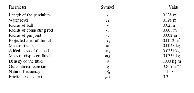
. A servo-actuator controlled the stroke frequency and amplitude of the plate (see figure 1). Two Nema 17 motors with a holding torque of 4.2 kg cm rotated a rack and pinion mechanism that converted the rotational motion into the linear motion of the plate. A bed of stone pellets at the other end of the channel acted as a damper to minimise wave reflection and ensure the formation of travelling surface waves. A pendulum with a bob diameter,
 $d=$
4 cm and a length,
 $l$
= 13.8 cm (distance between the centre of the bob and the hinge), was vertically mounted from the centre to the bottom wall of the channel. The pendulum is allowed to oscillate only in the vertical plane, and all other degrees of freedom are arrested. The pendulum consisted of a plastic ball with a density of
 $910 \, \text {kg m}{^-}{^3}$
and an iron rod of diameter 2 mm and density of
 $7800 \, \text {kg m}{^-}{^3}$
(summary of experimental parameters; see table 1). The contrast in densities between the ball and water renders the pendulum buoyant. In an undisturbed situation, the pendulum remains vertical, and when the surface waves are brought about by the actuation of the wave-maker plate, the pendulum exhibits oscillatory motion, which is the focal point of our investigation.
Schematic of the experimental set-up.

A high-speed camera (Phantom v7.3) with a resolution of 2048
 $\times$
2048 pixels captured the videos of the water wave and the pendulum motion at 100 frames per second after the initial transients die down. The movies were postprocessed to measure the response of the system. The angular displacement (
 $\theta$
) and frequency (
 $f_p$
) of the pendulum, along with the characteristics of the water wave such as wavelength (
 $ \lambda$
), frequency (
 $\Omega$
) and amplitude (
 $A$
), were computed using image analysis with in-house MATLAB programmes. The greyscale frames of the recorded videos were converted into binary images using a grey threshold. The MATLAB programmes extracted the time-series data of the relevant parameters from the subsequent frames of the video. The spatial resolution of the images for measuring the bob displacement and wave surface elevation varied from
 $3.5 \times 10^{-5} \, \text {to} \, 4.9 \times 10^{-4} \, \text {m pixel}{^-}{^1}$
.
This study employed the PIV technique to capture instantaneous 2-D velocity fields of the fluid motion around the oscillating pendulum. The velocity field is denoted by
 $ V (x, y, t)$
 $\equiv {u} \hat {\imath } + {v} \hat {\jmath }$
and represents the motion of the fluid at any point
 $ (x, y)$
at a specific time,
 $t$
. The unit vector
 $ \hat {\imath }$
denotes the direction parallel to the travelling wave (
 $x$
-axis), while
 $ \hat {\jmath }$
represents the direction perpendicular to the bottom of the liquid layer (the
 $y$
-axis). To visualise the flow, the water was seeded with neutrally buoyant tracer particles (14
 $\mu$
m diameter and density of 1700 kg m−3) coated with silver for better reflection. Although the density of the particles is higher than that of the fluid, their behaviour in suspension results in a very small slip velocity, approximately
 $7.4\times 10^{-5}$
ms−1 in water (Faleiros et al. Reference Faleiros, Tuinstra, Sciacchitano and Scarano2021; Aashish et al. Reference Aashish, Deepu and Kumar2024). This minimal slip velocity indicates that it is negligible, allowing the tracer particles to faithfully follow the fluid particles. Moreover, the primary aim of presenting the PIV results is to demonstrate that the observed subharmonic resonance is not due to a subharmonic characteristic of the velocity field, as discussed later, rather than to conduct a comprehensive turbulence analysis. The field of view encompassed a vertical, longitudinal plane measuring 228.8 mm
 $\times$
228.8 mm, illuminated by a continuous wave Nd-YAG laser operating at a frequency of 15 Hz. The laser light is reflected from a mirror positioned below the water channel at a
 $45^\circ$
angle to the horizontal plane, creating a laser sheet in the longitudinal plane of the pendulum. The seeded particle images were recorded using the same high-speed camera mentioned above. We set it to capture two frames within a time interval of 20 ms to record particle displacements for velocity calculations. We acquire a series of 150 image pairs at a sampling rate of 10 pairs per second. After capturing image pairs, they are divided into small interrogation windows, each measuring 104
 $\times$
104 pixels with a 50
 $\%$
overlap. A cross-correlation algorithm, executed using discrete Fourier transform (DFT), is applied within each window to determine particle displacement. This displacement data are processed using the postprocessing software (Insight 4G developed by TSI Inc) to calculate the velocity vectors. This method is applied to all interrogation windows, resulting in 2-D velocity vectors for each instantaneous flow field. Our observations revealed an average surface wave wavelength of the order of 10 cm. This value significantly exceeds the capillary length scale, a characteristic dimension associated with surface tension effects. This substantial difference confirms that the waves observed in this experiment are primarily driven by gravitational forces, classifying them as gravity waves (Kundu et al. Reference Kundu, Cohen and Dowling2015). The experiments explored a range of values for wavelength (
 $\lambda$
), wave frequency (
 $\Omega$
) and wave amplitude (
 $A$
) at a fixed water layer height of
 $H=198$
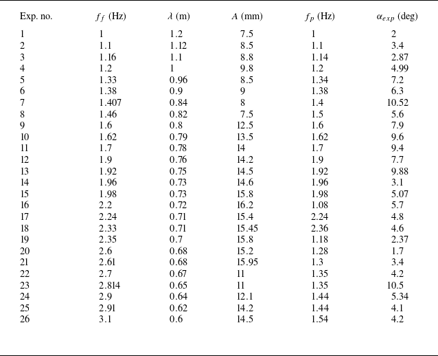
mm (see table 2). The experimental data in table 2 present wave frequencies (second column), wavelengths (third column) and amplitudes (fourth column), along with the response frequency and amplitude of the pendulum (fifth and sixth columns, respectively). It is evident from the data that as the forcing frequency varies, the response amplitude of the pendulum changes accordingly. Notably, the amplitude peaks at a forcing frequency of 1.4 Hz (Exp. no. 7), which aligns with the natural frequency of the pendulum and indicates primary resonance. As the forcing frequency increases, the response amplitude peaks at 2.81 Hz (Exp. no. 23). This frequency is close to twice the natural frequency of the pendulum, suggesting the occurrence of subharmonic resonance. In the experiment, the frequency and amplitude range of the wave-maker plate were carefully chosen to achieve linear, travelling, sinusoidal gravity waves. Linearity of the waves was ensured by focusing on waves where the amplitude-to-depth ratio
 $(A/H)$
was considerably lower than unity. However, very small amplitudes were avoided to maintain a measurable response from the pendulum. Data collection commenced after the transient effects subsided. The oscillation of the travelling wave velocity field exerts a periodic force on the pendulum, allowing us to model it as a forced nonlinear oscillator, as explained in the following section.
Summary of experimental parameters.

Experimental data and response amplitude of pendulum.

(Panels (a), (b), (c), (g), (h) and (i) present experimentally obtained time series, and their corresponding DFT are (d), (e), (f), (j), (k) and (l), respectively. Panels (a)–(f) depict the primary resonance case at
 $\Omega =0.9\omega _0$
(a) and (d),
 $\Omega =\omega _0$
(b) and (e), and
 $\Omega =1.1\omega _0$
(c) and (f). Panels (g)–(l) illustrate subharmonic resonance at
 $\Omega =1.9\omega _0$
(g) and (j),
 $\Omega =2\omega _0$
(h) and (k), and
 $\Omega =2.1\omega _0$
(i) and (l).

3. Experimental observation
Figure 2 presents the experimentally obtained time series and their corresponding DFT. Figures 2(d), 2(e) and 2(f) show DFT for three forcing frequencies (
 $f_f={\Omega }/{2\pi }$
): 1.33 Hz, 1.4 Hz and 1.5 Hz (Exp. nos. 5, 7 and 8; see table 2). Analysing these DFT, we observe a dominant peak in the frequency domain for each case, closely aligned with the respective forcing frequency. But the most prominent peak appears in the second case figure 2(e). This peak signifies a state of primary resonance, where the driving frequency excites a strong response at the same frequency close to the natural frequency (
 $f_0={\omega _0}/{2\pi }=1.4$
Hz) of the pendulum. Notably, the DFT consistently reveal a single, prominent peak centred precisely around the excitation frequency. This finding highlights the pronounced resonance effect when the driving frequency matches the natural frequency of the pendulum. In contrast, the DFT in figures 2(j), 2(k) and 2(l) reveal two dominant peaks in the frequency domain for forcing frequencies
 $(f_f)$
of 2.7, 2.81 and 2.9 Hz (Exp. nos. 22, 23 and 24 of table 2). Interestingly, the dominant peak in each case appears closely aligned with half the respective forcing frequency, which is near the natural frequency (1.4 Hz). However, a less prominent second peak centred around the forcing frequency exists for each case. This provides strong evidence of subharmonic resonance conditions in the examined oscillating system. To understand whether the forcing flow field can explain this behaviour of the pendulum, we delve into the velocity field itself. We employ PIV analysis for this purpose, which enables us to visualise the instantaneous velocity and vorticity fields surrounding the oscillating pendulum.
Figures 3 and 4 present the PIV analysis, depicting the phase-averaged 2-D velocity fields and vorticity fields in figures 3(a,c,e,g) and 4(a,c,e,g,i,k,m,o), alongside the corresponding potential flow solutions in figures 3(b,d,f,h) and 4(b,d,f,h,j,l,n,p) to assess the agreement between theoretical predictions and experimental observations, captured at key moments within the oscillation cycle for the primary and subharmonic resonance cases, respectively. (For details on the adopted phase-averaging method, readers are referred to Hashiehbaf & Romano (Reference Hashiehbaf and Romano2020).) For subharmonic resonance, the range is 0.00015 ms−1 to 0.034 ms−1. Additionally, the PIV results depict the intensity of vorticity using a colourmap. To enhance clarity, the surface wave and the pendulum (represented by a white sphere) are overlaid onto the PIV results, allowing for direct observation of the flow patterns concerning the motion.
Panels (a), (c), (e) and (g) display the phase-averaged 2-D velocity fields and vorticity captured via PIV, while the corresponding panels (b), (d), (f) and (h) illustrate the potential flow field, for primary resonance at four key instants:
 $t = 0$
,
 $ {T}/{4}$
,
 ${T}/{2}$
and
 ${3T}/{4}$
, respectively (where
 $T$
represents the wave oscillation period). The longest velocity vector corresponds to 0.014 ms−1. Parameters used were
 $f_f = 1.2$
Hz,
 $\lambda = 1$
m and
 $A = 0.0098$
m. The horizontal red line in images in panels (b), (d), (f) and (h) shows the chosen frame height in PIV.

In the primary resonance case, at
 $t = 0$
, the pendulum is at its equilibrium axis, and the wave velocity vector points to the left (highlighted by a red rectangle). As the pendulum swings, the wave velocity vector changes direction accordingly, mirroring the motion. In each quarter of the oscillation, the velocity field turns
 $90^\circ$
, as shown in figure 3 (also see ‘Movie 1.mp4’ in the Supplementary material, which shows instantaneous velocity vectors). One complete cycle of the wave velocity field coincides with one full swing of the pendulum, indicating that the wave frequency and the pendulum frequency are equal, as expected (
 $f_f=f_p$
). The potential flow velocity fields reveal similar dynamics of the velocity vectors (far away from the pendulum) as explained above. The overall structure and magnitude of the velocity field show a good match between the experimental PIV results and theoretical results. However, as expected, the PIV results depict weak disturbances in the flow field near the pendulum location. These disturbances are minimal and very close to the pendulum. This affirms our assumption of using potential flow to model the surrounding velocity field as a first-order approximation.
Panels (a), (c), (e), (g), (i), (k), (m) and (o) display the phase-averaged 2-D velocity fields and vorticity captured via PIV, while the corresponding panels (b), (d), (f), (h), (j), (l), (n) and (p) illustrate the potential flow field for subharmonic resonance at eight key moments:
 $t = 0, ({T}/{4}), ({T}/{2}), ({3T}/{4}), {T}$
,
 ${5T}/{4}$
,
 ${3T}/{2}$
and
 ${7T}/{4}$
. Parameters are
 $\Omega =2.61$
Hz,
 $\lambda =0.68$
m and
 $A=0.01595$
m.

In contrast to the primary resonance case, the PIV analysis for subharmonic resonance reveals a distinct interplay between the wave velocity field and the motion of the pendulum (refer to figure 4 and also see ‘Movie 2.mp4’ in the Supplementary material). While the wave velocity vector still exhibits identical directional changes, the frequency of these changes differs from the swing frequency of the pendulum. Here, the wave velocity field completes two full cycles (i.e. undergoes eight
 $90^\circ$
rotations) within the timeframe it takes for the pendulum to complete a single swing. Hence, the PIV analysis confirms that the forcing frequency is indeed twice the natural frequency of the pendulum (
 $f_f=2f_p$
), and the velocity field is devoid of any other harmonics. Note that this type of subharmonic resonance is a hallmark of parametrically excited oscillators (Nayfeh & Mook Reference Nayfeh and Mook2008). Also, the PIV images reveal the disturbed velocity field in close proximity to the buoyant pendulum. This disturbed field is characterised by irregular flow patterns resulting from the influence of the pendulum on the surrounding fluid. Additionally, stronger vortices are shed around the moving pendulum during this resonance as compared with primary resonance case. However, these vortices are not very prominent and consistent (as compared with, e.g. von Kármán vortex street) and thus are expected to be the effect of pendulum motion rather than its cause. Further, similar to the primary resonance, the potential flow solution shows good agreement with the PIV results in capturing both the rotational behaviour of the velocity vectors and the overall velocity field. However, subtle differences in the velocity field persist due to the exclusion of the motion pendulum effects in the potential flow model in both the resonance cases. For this resonance, stronger disturbances are observed near the pendulum, which is attributed to the shorter wavelength compared with the bob diameter. These findings challenge the one-way coupling assumption made in our theoretical model. Nonetheless, it is important to note that the region influenced by the motion of the pendulum is minimal. Thus, the potential flow solution remains a reliable first-order approximation for representing the velocity field.
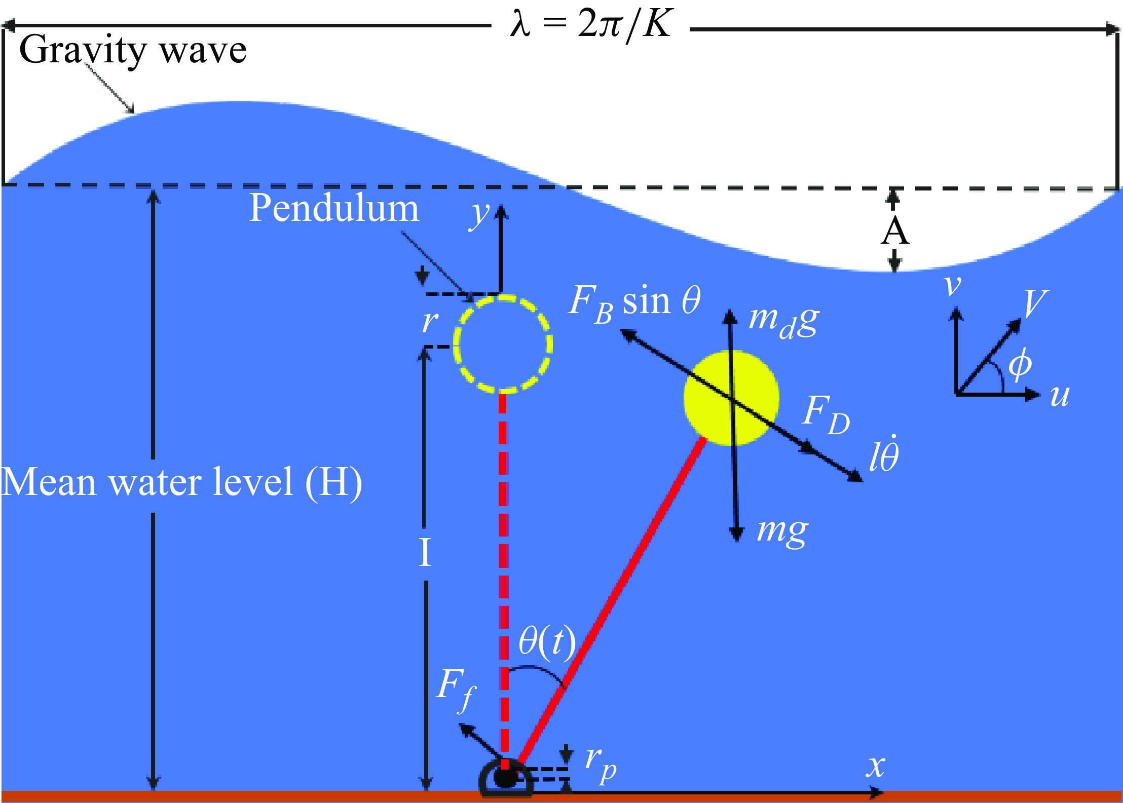
Schematic diagram of the system, defining key parameters at an instant when the pendulum swings towards the right and
 $u \gt l \dot {\theta }$
.

4. Analytical solution
We develop a theoretical model to capture the dynamics of a buoyant pendulum and understand the interaction between the waves and the pendulum, which is oriented perpendicularly to linear gravity waves on a water layer with a mean depth
 $H$
, as depicted in figure 5. The pendulum undergoes oscillations due to the effect of gravity waves on the free surface, which has a sinusoidal shape with frequency
 $\Omega$
, amplitude
 $A$
and wavelength
 $\lambda = {2\pi }/{K}$
, where
 $K$
is the wavenumber. The spatial coordinate
 $x$
is aligned with the wave propagation direction, and the coordinate
 $y$
is perpendicular to the bottom surface. We assume the wave has a small amplitude (
 $A$
) and a small slope (
 $A/\lambda$
). We also assume that the fluid is inviscid, irrotational and incompressible, so we can use the potential flow equation to find the fluid velocity components. The
 $x$
and
 $y$
component of the fluid velocity in the limit of small (
 $A/H$
) is given by (Kundu et al. Reference Kundu, Cohen and Dowling2015)
 \begin{gather} u = \frac {A\Omega \cosh (Ky)}{\sinh (KH)} \cos (Kx - \Omega t), \end{gather}
 \begin{gather} v = \frac {A\Omega \sinh (Ky)}{\sinh (KH)} \sin (Kx - \Omega t). \end{gather}
The velocity component of the fluid tangent to the pendulum is expressed as
 \begin{equation} V_t = V \cos (\theta +\phi ), \end{equation}
where
 \begin{equation} V = \sqrt {u^2 + v^2}, \quad \phi = \tan ^{-1}\left (\frac {v}{u}\right ). \end{equation}
Given a small wave slope and a small pendulum displacement, it is reasonable to assume that the tangential velocity of the pendulum aligns with the
 $x$
-component of the wave velocity. This simplification is justified as the linear wave and minimal pendulum swing result in limited angular deviations, leading to a near-parallel alignment between the tangential velocity and the horizontal component of the fluid motion. The equation of motion governing the behaviour of the pendulum is derived by applying the principle of conservation of angular momentum about the hinge point, which takes into account various torques acting on the bob of the pendulum and is given by
 \begin{equation} (m + m_a) l^2 \ddot {\theta }+F_B \sin {\theta }l = \frac {1}{2} A_p C_D \rho \left | u - l \dot {\theta } \right | ( u - l \dot {\theta })l -F_f\times r_p \end{equation},
where
 $\theta$
denotes the angular position of the pendulum from its vertical equilibrium position and
 $\dot {()}$
denotes the derivative with respect to time. The forces
 $F_B$
and
 $F_f$
represent the buoyant force and frictional force at the hinge, respectively, and
 $C_D$
denotes the drag coefficient. The friction force for small angular displacement, is
 $F_f= {\mu }_f g (m_d - m) sgn (\dot {\theta })$
. The friction force is further linearised using the approach proposed by Byrtus et al. (Reference Byrtus, Hajžman and Zeman2013). This approach involves approximating the signum function, sgn
 $(\dot {\theta })$
, as a linear term
 $ ({4}/{\pi (a \omega _0)}) (\dot {\theta })$
. Here,
 $a$
and
 $\omega _0$
represent the constants, which are the maximum amplitude and frequency of the pendulum, respectively. Although the amplitude
 $a$
is unknown at this stage, it is modelled using the maximum response amplitude observed in all experiments. The detailed information of other key parameters, including the length of the pendulum (
 $l$
), radius of the ball (
 $r$
), radius of the pin joint (
 $r_p$
), mass of the ball (
 $m$
), added mass (
 $m_a$
) and density of the fluid (
 $\rho$
) is provided in table 1.
The left-hand side of (4.4) consists of two terms: one representing the torque resulting from the inertia of the bob and the other denoting the torque generated by a buoyant force acting upon it. The right-hand side comprises two terms: the first one represents the torque exerted by drag force exerted by the oscillatory flow around the bob, and the second one indicates the torque induced by friction force at the hinge joint (Mathai et al. Reference Mathai, Loeffen, Chan and Wildeman2019). Given a small angular displacement, the equation of motion (4.4) is rewritten as
 \begin{equation} (m + m_a)l^2\ddot {\theta }+ (m_d - m)gl\sin \theta ={\frac {1}{2}} A_p C_D \rho u_{tip}(u-l{\dot \theta })l - {\mu }_e g (m_d - m) (\dot {\theta }) r_p, \end{equation}
where the parameters
 $m_d$
,
 $g$
and
 ${\mu }_e= ({4{\mu }_f}/{\pi (a \omega _0)})$
denote the mass of the displaced fluid, gravitational acceleration, effective friction coefficient and the friction coefficient, respectively, which are listed in table 1. Here
 $u$
is evaluated at
 $x=l\sin \theta$
and
 $y=l\cos \theta$
. Note that the drag force on the right-hand side, the penultimate term in (4.4), is proportional to the square of relative velocity. However, in order to keep the theoretical analysis simpler, our model incorporates a linearised drag term (right-hand side, penultimate term in (4.5)) similar to the one employed in Mullarney & Henderson (Reference Mullarney and Henderson2010). However, a key distinction lies in the definition of the characteristic velocity. While Mullarney & Henderson (Reference Mullarney and Henderson2010) used a different scale, we use the peak fluid velocity at the undisturbed location of the bob centre of the pendulum (
 $y = l$
),
 $u_{tip}$
as the velocity scale for linearising the drag force (for more details, refer to Kumar et al. Reference Kumar, Kumar, Deepu and Ramya2021). The linearisation holds well when the wave amplitude exceeds the pendulum displacement (Gudmestad & Connor Reference Gudmestad and Connor1983), and this condition is satisfied in most scenarios for our case. Near resonances, where this criterion is not strictly met, the assumption continues to offer a reasonable approximation. Any inaccuracies arising from this assumption are minimal and do not impact the key dynamics, as demonstrated later by the satisfactory agreement between the experimental and analytical results. To further validate this approach, we performed a detailed numerical solution of the theoretical model, both with and without the linearised drag force. The results reveal minimal differences less than two degrees in the response amplitude of the pendulum, even in resonance regions (results not shown). Consequently, while simplified, the assumption facilitates a tractable analytical solution via the method of MMS while preserving the essential system dynamics. From (4.1a
), we get
 \begin{equation} u_{tip} = \frac {A\Omega \cosh (Kl)}{\sinh (KH)}. \end{equation}
The viscous effects will be dominant near the bottom wall of the tank, which thus justifies the use of the potential flow approximation. Mullarney & Henderson (Reference Mullarney and Henderson2010) suggest that this viscous layer has a thickness of
 $\delta _v$
, which scales with the square root of the kinematic viscosity (
 $\nu$
) and inversely with the wave frequency (
 $\Omega$
). Given typical values of kinematic viscosity (
 $\nu \approx 10^{-6} \, \text {m}^2\,\text {s}^{-1}$
) and wave frequency (
 $\Omega \approx 10 \, \text {s}^{-1}$
),
 $\delta _v$
becomes approximately
 $10^{-2} \, \text {m}$
. The relatively small thickness of this viscous layer compared with the overall water depth (
 $H$
) allows us to assume that most of the fluid behaves as an inviscid region for our analysis.
To achieve a non-dimensionalised form of the equation of motion, we employ characteristic scales of
 $l$
for length,
 $1/\omega _0$
for time (where
 $ \omega _0= \sqrt {\frac {(m_d - m)g}{(m + m_a)l}}$
represents the linear natural frequency of the pendulum) and
 $l\omega _0$
for velocity. Hence, non-dimensionalising the parameters as
 $x^* = { {x}/{l}}$
,
 $y^* = {{y}/{l}}$
,
 $t^* = {t}{\omega _0}$
,
 $u^* = { {u}/{ l \omega _0}}$
,
 $H^* = { {H}/{l}}$
,
 ${K^*}= {K}{l}$
,
 $ {A^*}= {{{A}}/{l}}$
and
 $ {\Omega ^*}= {{\Omega }/{\omega _0}}$
. By putting (4.1a
) and (4.6) in (4.5) and non-dimensionalising it and upon further simplification, one obtains
 \begin{equation} {\begin{aligned} &\frac {{\textrm {d}}^2 \theta }{{\textrm {d}}t^*{}^2} + \sin \theta + \Omega \left ( \frac { A \cosh (K^*)}{2\sinh (K^*H^*)} \frac {A_p l C_D \rho }{m + m_a} + \frac {4{\mu }_f r_p^* }{\pi a \Omega ^*} \right ) \frac {{\textrm {d}}\theta }{{\textrm {d}}t^*}= \frac {A^* \Omega ^* \cosh (K^*)}{2\sinh (K^* H^*)}\\ & \left ( \frac {A_p C_D \rho l}{m + m_a} \right ) \times \frac {A^* \Omega ^* \cosh (K^*)}{\sinh (K^* H^*)} \cos (K^* \sin \theta - \Omega ^* t^*).\end{aligned}} \end{equation}
By dropping (*), (4.7) can now be written as
 \begin{equation} \frac {{\textrm {d}}^2 \theta }{{\textrm {d}}t^2} + \sin \theta +\Omega \zeta \frac {{\textrm {d}}\theta }{{\textrm {d}}t} =\Omega ^2 \psi \cos (K\sin \theta - \Omega t). \end{equation}
Here, the dimensionless damping coefficient attributed by fluid drag and friction at the pin joint of the pendulum is denoted by
 $\zeta$
. The magnitude of the periodic excitation due to drag of the gravity wave is represented by
 $\psi$
and
 $\Omega$
indicates dimensionless excitation frequency. Here
 $\zeta$
and
 $\psi$
are given by
 \begin{equation} \zeta =\frac { A \cosh (K)}{2\sinh (KH)} \frac {A_p l C_D \rho }{m + m_a} + \frac {4{\mu }_f r_p }{\pi \alpha \Omega }, \quad \psi = \frac {lA^2 \cosh ^2(K)}{2\sinh ^2(KH)} \left ( \frac {A_p C_D \rho }{m + m_a} \right ). \end{equation}
Taylor expanding the
 $\sin \theta$
term appearing on both sides of (4.8) up to the third order, given the small oscillation amplitudes observed in our experiment (with a maximum
 $\theta$
of 0.21 radians), results in
 \begin{equation} \frac {{\textrm {d}}^2 \theta }{{\textrm {d}}t^2} + \left(\theta - \frac {\theta ^3}{3!}\right) + \Omega \zeta \frac {{\textrm {d}}\theta }{{\textrm {d}}t} =\Omega ^2 \psi \cos \left [\left(K\theta - \frac {K\theta ^3}{3!}\right) - \Omega t\right ]. \end{equation}
Using a trigonometric identity, (4.10) can be rewritten as
 \begin{align} &\frac {{\textrm {d}}^2 \theta }{{\textrm {d}}t^2} + (\theta - \frac {\theta ^3}{3!}) + \Omega \zeta \frac {{\textrm {d}}\theta }{{\textrm {d}}t} \nonumber\\ &\qquad = \Omega ^2 \psi \left [ \cos \left(K\theta - \frac {K\theta ^3}{3!}\right)\cos (\Omega t) + \sin \left(K\theta - \frac {K\theta ^3}{3!}\right)\sin (\Omega t) \right ]. \end{align}
Again, using the fact that
 $\theta$
is very small, we make the following approximations:
 $\cos (K\theta - ({K\theta ^3}/{3!})) \approx \cos (K\theta )$
and
 $\sin (K\theta - ({K\theta ^3}/{3!})) \approx \sin (K\theta )$
. Thus, (4.11) reduces to
 \begin{equation} \frac {{\textrm {d}}^2 \theta }{{\textrm {d}}t^2} + \left(\theta - \frac {\theta ^3}{3!}\right) + \Omega \zeta \frac {{\textrm {d}}\theta }{{\textrm {d}}t} = \Omega ^2 \psi \left [ \cos (K\theta )\cos (\Omega t) + \sin (K\theta )\sin (\Omega t) \right ]. \end{equation}
Further, Taylor expanding
 $\cos (K\theta )$
and
 $\sin (K\theta )$
appearing on the right-hand side in (4.12) and retaining terms up to the third power and upon simplification, we get
 \begin{align} &\ddot {\theta } + (1 - \Omega ^2 \xi \sin (\Omega t))\theta + \Omega \zeta \dot {\theta } + \Omega ^2 \mu \cos (\Omega t)\theta ^2 + \left(\Omega ^2 \eta \sin (\Omega t) - \frac {1}{6}\right)\theta ^3 \nonumber\\ &\qquad =\Omega ^2 \psi \cos (\Omega t), \end{align}
where
 $\xi =\psi k$
represents the magnitude of the parametric excitation associated with the cyclic variation in drag induced by gravity waves. Due to this parametric excitation, it is not surprising that the system exhibits a subharmonic resonance, as explained later. The coefficients,
 $\mu$
and
 $\eta$
associated with quadratic and cubic nonlinearities, respectively, arising from gravity waves are given by
 \begin{equation} \mu = \frac {\psi (K)^2}{2!}, \quad \eta = \frac {\psi (K)^3}{3!}. \end{equation}
Approximate solutions to (4.13) are obtained through the utilisation of MMS (Rand Reference Rand2005; Nayfeh & Mook Reference Nayfeh and Mook2008). This theoretical analysis reveals the existence of multiple resonance conditions within the system. Specifically, we focus on two key resonance regimes, which are when the wave frequency approaches the natural frequency (primary resonance) of the pendulum and subharmonic resonance (when the wave frequency is near twice the natural frequency). Our experimental investigation also confirms the theoretical observation about primary and subharmonic resonance phenomena, as elaborated in the forthcoming section.
4.1. Primary resonance
In this section, we investigate the steady-state response amplitudes of the pendulum excited by surface gravity wave with a frequency close to the natural frequency of the pendulum.
4.1.1. Perturbation analysis
Since MMS is a perturbation method, one requires that the nonlinear terms are less dominant than the linear terms. Thus, it is essential to gauge the order of magnitude of each term in the nonlinear equation. To this end, we turn our attention to the experimental conditions at the primary excitation (Exp. no. 7; table 2). The order of magnitude of different terms in (4.13) is given in table 3. As can be noted, the response amplitude of the pendulum (
 $\theta$
), dimensionless excitation frequency (
 $\Omega$
) and excitation amplitude (
 $\psi$
) are of the order
 $10^{-1}$
,
 $1$
and
 $10^{-2}$
, respectively. Despite its apparent insignificance, this excitation triggered substantial responses, suggesting a low-order excitation, which is termed as ‘
 $\text {weak excitation}$
’. Subsequently, we consider
 $\psi$
to be of the order
 $\epsilon$
(the small non-dimensional bookkeeping parameter to be used in MMS), which is of order
 $10^{-2}$
and reorder
 $\psi$
as
 $\psi = \epsilon \hat {\psi }$
. Furthermore, we noted in the experiment (table 2) that the magnitude of damping and nonlinear terms is also relatively smaller than terms describing inertia and stiffness. Terms lower than the second order will have progressively less influence on the dynamic behaviour, owing to their relatively smaller order of magnitude. Hence, adopting a more general approach, we include these lower-order terms also at the
 $O$
(
 $\epsilon$
) level, leading us to express
 $\xi$
,
 $\zeta$
,
 $\chi$
,
 $\mu$
and
 $\eta$
as
 $\epsilon \hat {\xi }$
,
 $\epsilon \hat {\zeta }$
,
 $\epsilon \hat {\chi }$
,
 $\epsilon \hat {\mu }$
and
 $\epsilon \hat {\eta }$
, respectively. Introducing these rescalings and simplifying the notation by omitting the over-hat on these variables, the nonlinear equation of motion is rewritten as
 \begin{align} &\ddot {\theta } + (1 -\epsilon \Omega ^2 \xi \sin (\Omega t))\theta + \epsilon \Omega \zeta \dot {\theta } + \epsilon \Omega ^2 \mu \cos (\Omega t)\theta ^2 + \epsilon \left(\Omega ^2 \eta \sin (\Omega t) - \frac {1}{6}\right)\theta ^3 \nonumber\\ & \quad =\epsilon \Omega ^2 \psi \cos (\Omega t). \end{align}
The order of magnitude obtained experimentally for the terms in (4.13) at primary resonance.

This equation incorporates several dimensionless parameters:
 $\xi$
represents the frequency ratio,
 $\zeta$
is the damping ratio,
 $\mu$
is the dimensionless coefficient of quadratic nonlinearity,
 $\eta$
is the dimensionless coefficient of cubic nonlinearity and, finally,
 $\psi$
denotes the dimensionless excitation. Following the MMS approach, we seek an approximate solution to (4.15) in the form of a uniform asymptotic expansion given as (Nayfeh & Mook Reference Nayfeh and Mook2008)
 \begin{equation} {\theta }={\theta }_0 \left (T_0,T_1\right ) + \epsilon {\theta }_1 \left (T_0,T_1\right ). \end{equation}
Here we introduced two different time scales to analyse the behaviour of the system. The first scale, denoted by
 $T_0$
, represents the fast time scale and is equivalent to the original time variable
 $t$
. The second scale, denoted by
 $T_1$
, represents the slow time scale and is defined as
 $\epsilon t$
. To analyse the dynamics on these time scales, we define the partial derivatives
 $D_0$
and
 $D_1$
as follows:
 $D_0$
denotes differentiation with respect to
 $T_0$
, and
 $D_1$
denotes differentiation with respect to
 $T_1$
(Nayfeh & Mook Reference Nayfeh and Mook2008).
Further, we introduce the detuning parameter
 $\sigma$
to quantify the closeness of the excitation frequency to the natural frequency of the system (
 $\omega _0$
). Hence, the condition for primary resonance is presented as
 \begin{equation} \Omega = 1 + \epsilon \sigma . \end{equation}
By applying the primary resonance condition, as provided in (4.17)–(4.15), and disregarding terms of order higher than
 $\epsilon$
, as we are focusing on a first-order approximation here, we rewrite (4.15) as follows:
 \begin{align} \ddot {\theta } &+ (1 - \epsilon \xi \sin (T_0 + \sigma T_1))\theta +\epsilon \zeta \dot {\theta } + \epsilon \mu \cos (T_0 + \sigma T_1)\theta ^2 + \epsilon \!\left(\! \eta \sin (T_0 + \sigma T_1) - \frac {1}{6}\!\right)\!\theta ^3 \nonumber\\ &= \epsilon \psi \cos (T_0 + \sigma T_1). \end{align}
Upon substituting the ansatz from (4.16) into (4.18) and considering similar powers of
 $\epsilon$
we obtain
 \begin{align} &\epsilon ^{0} \rightarrow D_{0}^{2}\theta _{0} + \theta _{0} = 0, \end{align}
 \begin{align} \begin{split} &\epsilon ^{1} \rightarrow D_{0}^{2} \theta _{1} + \theta _{1} + \zeta D_{0}{\theta }_{0} + 2D_{0} D_{1} \theta _{0} - \xi \sin ( T_0 + \sigma T_1) \theta _{0} \\ &\qquad + \mu \cos ( T_0 + \sigma T_1) \theta _{0}^2 + \left(\eta \sin ( T_0 + \sigma T_1) - \frac {1}{6}\right) \theta _{0}^3 = \psi \cos ( T_0 + \sigma T_1). \end{split} \end{align}
Equation (4.19a ) presents the solution for the free vibration of the pendulum, an undamped and linear system. Therefore, the general solution of the equation can be written as
 \begin{equation} \theta _0 = \mathcal {A}\left (T_1\right ){\textrm {e}}^{{\textrm {i}}T_0}+{\textrm {c.c.}} \end{equation}
Here, notation ‘c.c.’ denotes the complex conjugate of preceding terms. Here
 $\mathcal {A}(T_1)$
, dependent on the slow time scale
 $T_1$
, is complex-valued and determined by enforcing the solvability condition at first order and the overbar signifies the complex conjugate
 $(\bar {\mathcal {A}} (T_1 ))$
. Substituting (4.20) into (4.19b
) and expressing the sine and cosine terms in their exponential forms, we arrive at (A1) in Appendix A.1.1, where detailed intermediate steps are provided. Following the simplifications of (A5a
) and (A5b
) for the steady-state solution detailed in Appendix A.1.1, we derive the frequency response equation as follows:
 \begin{eqnarray} &(4\zeta \alpha )^2 (4\psi - 3\mu \alpha ^2)^2 + (4\psi - \mu \alpha ^2)^2 (0.5\alpha ^3 + 8\sigma \alpha )^2 \nonumber \\ &\qquad - (4\psi - \mu \alpha ^2)^2 (4\psi - 3\mu \alpha ^2)^2 = 0. \end{eqnarray}
Equation (4.21) establishes the relation between the response amplitude and the detuning parameter,
 $\sigma$
, under steady-state conditions. Solving for
 $\sigma$
, we obtain
 \begin{equation} \sigma = \frac {-0.5\alpha ^3 \pm (4\psi - 3\mu \alpha ^2) \sqrt {1 - \left (\frac {4\zeta \alpha }{4\psi - \mu \alpha ^2}\right )^2}}{8\alpha }. \end{equation}
Similarly, phase (
 $\gamma$
) can be obtained as
 \begin{equation} \tan \gamma = -\frac {4\zeta }{(0.5\alpha ^2 + 8\sigma )} \times \frac {(4\psi - 3\mu \alpha ^2)}{(4\psi - \mu \alpha ^2)}. \end{equation}
Substituting (4.20) and (A3) into (4.16), the first-order approximation of the steady-state primary resonance can be obtained as
 \begin{equation} \theta = \alpha \cos (\Omega t - \gamma ) + O(\varepsilon ). \end{equation}
To obtain a first-order approximation of the steady-state primary resonance, we first insert a specific value of
 $\alpha$
into (4.22) and solve for
 $\sigma$
. Next, utilising (4.23), we obtain
 $\gamma$
, resulting in the first-order approximation of the steady-state primary resonance. Further, the stability analysis of the stationary solutions is discussed in Appendix A.1.2.
4.2. The
 ${1}/{2}$
subharmonic resonance

After examining primary resonance, we now turn our attention to the behaviour of the pendulum under the influence of surface gravity waves with frequencies higher than its natural frequency, particularly in the vicinity of twice the natural frequency. In this section, we introduce the subharmonic resonance condition, represented as
 \begin{equation} \Omega = 2 + \epsilon \sigma . \end{equation}
4.2.1. Perturbation analysis
In our experimental study of subharmonic excitation (Exp. no. 23; see table 2), we observed a markedly more intense excitation than what was seen at primary resonance, with the intensity being roughly an order of magnitude greater. When assessing the magnitude of various terms in (4.13) under the subharmonic condition, we employed a methodology akin to that described in § 4.1.1. Our findings indicated that the response amplitude of the pendulum
 $\theta$
, the non-dimensional frequency of excitation
 $\Omega$
, and the amplitude of excitation
 $\psi$
are approximately of the order
 $10^{-1}$
,
 $1$
and
 $10^{-1}$
, respectively, as detailed in table 4. It was also observed that the damping and nonlinear terms are significantly lesser in magnitude, of the order
 $O(10^{-2})$
or smaller, when compared with the terms representing inertia, stiffness and excitation forces. We include all terms of the order
 $O(10^{-2})$
or smaller at
 $O(\epsilon )$
in the model; thus we rescale
 $\xi$
,
 $\zeta$
,
 $\mu$
and
 $\eta$
as
 $\epsilon \hat {\xi }$
,
 $\epsilon \hat {\zeta }$
,
 $\epsilon \hat {\mu }$
and
 $\epsilon \hat {\eta }$
respectively. In the following, we drop the over-hat from the rescaled variables to simplify the equation. Next, we apply the subharmonic condition as provided in (4.25) into (4.15). Since our approximation focuses on terms up to the order of
 $\epsilon$
, we consider terms containing powers of
 $\epsilon$
and discard higher-order terms. This approach allows us to capture the dominant effects in the behaviour of the system while simplifying the analysis by neglecting terms of order
 $\epsilon ^2$
and smaller.
Experimentally determined order of magnitude for terms in (4.13) at subharmonic resonance.

Following the approach used for primary resonance, the modulation equations, namely, (A14a
) and (A14b
) were derived, with detailed steps and intermediate equations provided in Appendix A.2. For the steady-state solution, we set
 $\alpha ^{\prime} = \gamma ^{\prime} = 0$
in (A14a
) and (A14b
), and upon further simplification, one obtains the following frequency response of the system under subharmonic resonance:
 \begin{align} &[64\mu\Lambda - 8\sigma - (8\Lambda^2 + \alpha^2)]^2 [4\xi - \eta(2\alpha^2 + 12\Lambda^2)]^2+ 16\zeta^2[16\xi - 4\eta(4\alpha^2 + 12\Lambda^2)]^2 \nonumber \\ & - [4\xi - \eta(2\alpha^2 + 12\Lambda^2)]^2[16\xi - 4\eta(4\alpha^2 + 12\Lambda^2)]^2 = 0. \end{align}
Equation (4.26) establishes the relation between the amplitude of the response and the detuning parameter,
 $\sigma$
, under steady-state conditions. Solving for
 $\sigma$
, we obtain
 \begin{equation} \sigma = \frac {64\mu \Lambda - (8\Lambda ^2 + \alpha ^2) \pm 4[4\xi - \eta (4\alpha ^2 + 12\Lambda ^2)] \sqrt {1 - \left (\frac {4\zeta }{4\xi - \eta (2\alpha ^2 + 12\Lambda ^2)}\right )^2}}{8}. \end{equation}
Similarly, phase
 $\gamma$
can be obtained as
 \begin{equation} \tan \gamma = \frac {(8\sigma + 8\Lambda ^2 + \alpha ^2 - 64\mu \Lambda )}{16\zeta } \times \frac {\left[4\xi - \eta \left(2\alpha ^2 + 12\Lambda ^2\right)\right]}{\left[4\xi - \eta \left(4\alpha ^2 + 12\Lambda ^2\right)\right]}. \end{equation}
By substituting (4.20) and (A10) in (4.16), one can obtain the first-order approximation of the steady-state subharmonic resonance as
 \begin{equation} \theta = \alpha \cos \left (\frac {\Omega t - \gamma }{2}\right ) + \Lambda \cos (\Omega t) + O(\varepsilon ). \end{equation}
Additionally, the stability of the derived stationary solutions is examined in Appendix A.2.2.
5. Theoretical results and discussion
This section delves into the results obtained from the mathematical modelling framework established in the preceding section. Our focus is on exploring the nonlinear oscillatory behaviour of a fully submerged buoyant pendulum experiencing lateral swings influenced by drag from surface gravity waves. To ensure the reliability of our findings, we validated the accuracy of our analytical results using MMS with numerical solutions. Additionally, we present the comparisons between our theoretical results and experimental observations within specific parameter ranges corresponding to primary and subharmonic resonances.
5.1. Primary resonance
Numerically (top row) and analytically (bottom row) obtained time series (left panel) and their corresponding DFT (right panel) at
 $\Omega =\omega _0$
for
 $\xi$
= 0.0155,
 $\zeta$
= 0.02,
 $\mu$
= 0.008,
 $\eta$
= 0.0028, and
 $\psi$
= 0.015.

This section examines the comparative analysis between numerical and analytical results. The steady-state angular position of the pendulum is depicted through time series analysis (figures 6
a and 6
c). Its corresponding frequency spectrum (figures 6
b and 6
d) was obtained through both numerical (figures 6
a and 6
b) and analytical (figures 6
c and 6
d) methods, based on the experimentally obtained data provided in table 2 (Exp. no. 7). All parameters were aligned with the experimental values, with a minor adjustment made only to the damping coefficient
 $\zeta$
to account for the influence of friction at the joints. The data were collected at a forcing frequency of 1.407 Hz, which is close to the natural frequency of the pendulum. Notably, the angular position amplitude exhibits negligible variation over the specified time interval, indicating a steady-state oscillation for both numerical and analytical results. To obtain the numerical solution, we integrated (4.13) using MATLAB ODE45 solver employing a fourth/fifth-order Runge–Kutta method. The integration ran up to
 $t = 9000$
s. Analysing the resulting time history of displacement, we applied a DFT to the final 6000 data points. Analytical solutions were obtained by solving the first-order approximate solution of (4.18) for the steady-state primary resonance, derived through the MMS, as expressed in (4.24).
The time series presented in figures 6(a) and 6(c) exhibit a characteristic pattern of recurring oscillations, signifying the periodic response of the system. These oscillations directly correspond to a prominent peak observed in the corresponding DFT depicted in figures 6(b) and 6(d). Notably, this prominent peak in the frequency domain is located at the forcing frequency of 1.407 Hz, which coincides with the natural frequency (
 $f_0$
) of the pendulum. This observation aligns perfectly with the condition of primary resonance, where the response of the system is most pronounced when the forcing frequency matches its natural frequency. This alignment serves as compelling evidence, confirming that the excitation frequency harmonises precisely with the natural frequency of the pendulum, as observed in the experimental results as well. As observed from the figures, the solution obtained using MMS exhibits slight deviations from the numerically calculated amplitude. These discrepancies likely stem from limitations associated with the MMS approach, which approximates the solution only up to the first order in
 $\epsilon$
. Additionally, the time history and DFT analysis for primary resonance presented here show a significant discrepancy from the experimental finding, as illustrated in figures 2(b) and 2(e). One potential explanation for the disparity observed lies in the uncertainty surrounding the drag coefficient (
 $C_D$
) and added mass coefficient (
 $C_m$
). The experiments yield a Reynolds number (
 $Re \approx 1500$
) and an acceleration number (
 $An \approx 1.6$
) for the primary resonance. Consequently, we chose
 $C_m = 0.75$
and
 $C_D = 2.5$
based on the work of Karanfilian & Kotas (Reference Karanfilian and Kotas1978). The discrepancy is also influenced by the chosen value of
 $\zeta$
, which contributes to the overall uncertainty in the model. However, a detailed discussion on the uncertainty associated with these coefficients, possible ways to minimise the discrepancy, and other potential contributing factors is presented in the upcoming § 5.2.
Comparison between numerically and analytically obtained frequency responses for primary resonance (refer to figure 6 caption for the parameter values used). Blue dots represent stable solutions, while red line indicate unstable solutions obtained using MMS. Black circles and magenta stars denote numerical backward and forward sweeps, respectively. The vertical dash–dot lines indicate the frequency ratios selected for further analysis. Here I.P. denotes intersections of these frequency ratio lines with the response curve, and B.P. represents bifurcation points. Arrows pointing up and down show jump-up and jump-down phenomena, respectively.

Further, to understand the behaviour of the system near primary resonance, we obtain the analytical solutions from the frequency response equation (4.22). While the analytical solution offers valuable insights, it is essential to assess its accuracy. Therefore, we also obtain a numerical solution by solving the second-order nonlinear ordinary differential equation (4.13) using the ODE45 routine in MATLAB. This numerical approach provides a more precise solution, serving as a validation tool for the analytical results.
Employing the analytical and numerical methods discussed earlier, figure 7 presents the frequency response plot. This plot presents the analytical solution obtained using the MMS. The transition between stable and unstable branches, known as bifurcation points, is marked by
 $B.P_1$
and
 $B.P_2$
. Additionally, the numerical solutions are overlaid, with magenta stars representing the forward frequency sweep and black circles representing the backward sweep. Three vertical maroon dash–dot lines highlight selected frequency ratios in three distinct regions labelled I, II and III for force response analysis, which will be discussed in detail in the following sections. These lines intersect the response curve at various points, as
 ${\rm I.P_1}$
to
 ${\rm I.P_5}$
. The analytical solution, depicted by a dotted marker, is obtained from the frequency response equation (4.22) with experimentally obtained non-dimensional parameters:
 $\xi$
= 0.0155,
 $\zeta$
= 0.02,
 $\mu$
= 0.008,
 $\eta$
= 0.0028 and
 $\psi$
= 0.015. The stability of the analytical solution of the system is evaluated using the stability criterion outlined in (4.22) of Appendix A.1.2. A positive eigenvalue signifies an unstable solution, leading to the unbounded growth of perturbations and the system potentially seeking a different stable state. Conversely, a negative eigenvalue ensures stability, where perturbations diminish, and the system returns to equilibrium. The figure shows the stable solution (marked in blue) and the unstable solution (marked in red) for different values of the frequency ratio
 $(\Omega /\omega _0)$
as the control parameter. The numerical results (shown in the figure by the black star marker) represent the amplitude of the steady-state solution of the nonlinear equation of motion, as given by (4.13) corresponding to a specific frequency ratio. The numerical and MMS solution agree well near
 $\Omega \approx \omega _0$
(resonance region) in figure 7, which displays the frequency response of the system. However, the agreement weakens as the forcing frequency
 $(\Omega )$
moves away from this region, with the MMS solution exhibiting slight deviations from the numerically calculated amplitude. This discrepancy may arise from approximating the solution using only two terms in the uniform expansion as outlined in (4.16). Enhancing the solution could potentially be achieved by incorporating additional terms into the expansion.
The figure shows that the response exhibits a jump phenomenon at distinct frequency ratios. This shows the presence of hysteresis in the system. The analytical solution also captures the stable and unstable branches; the solution also identifies the locations of the bifurcation points, denoted as
 ${\rm B.P._1}$
and
 ${\rm B.P._2}$
in the figure. The investigation utilises the frequency ratio as a controlling parameter and reveals an important trend: as the frequency ratio increases (forward sweeping), the amplitude of the motion of the pendulum increases until it reaches a critical juncture denoted as a point
 ${\rm B.P._2}$
(
 $\Omega /\omega _0$
= 0.975). At this critical point, a qualitative shift occurs: the previously stable response loses stability, transitioning into an unstable state. This characteristic transformation, marked by the loss of stability at point
 ${\rm B.P._2}$
, is recognised as a saddle-node bifurcation (Thomsen et al. Reference Thomsen, Thomsen and Thomsen2003). When the system reaches this critical point, the stable and unstable solutions merge. As the frequency ratio continues to increase beyond
 ${\rm B.P._2}$
, the response of the system switches to the higher amplitude solution because there are no other stable solutions nearby. However, when the direction of the sweep reverses (backward sweep), the pendulum maintains stable responses until it reaches another critical point,
 ${\rm B.P._1}$
 $(\Omega /\omega _0= 0.96)$
. Here, another saddle-node bifurcation occurs, causing the response to switch to the stable solution on the lower branch. The frequency response exhibits hysteresis due to the two saddle-node bifurcations. Furthermore, the figure reveals a leftward skew in the peak of the response curve, which suggests a softening effect. This softening behaviour can be attributed to the negative cubic nonlinear term
 $(\Omega ^2 \eta \sin (\Omega t) - ({1}/{6}))\theta ^3$
, which stems from the drag term as shown in (4.15). Here, the negative sign of
 $ {1}/{6}$
outweighs the product
 $\Omega ^2 \eta \sin (\Omega t)$
, which tends to be smaller due to the orders of magnitude involved (
 $\eta$
being
 $O$
(
 $10^{-3}$
) and
 $\Omega$
being
 $O$
(
 $1$
)). As a result, even if the product is positive, the negative constant term dominates. This consistent negativity induces a softening effect on the response of the system. In essence, this negative nonlinearity leads to a decrease in the stiffness of the pendulum as the amplitude of its motion increases.
Further, the figure sheds light on the response behaviour by categorising the frequency response plot into three distinct regions based on the potential response amplitude. Understanding these regions is crucial for various applications, particularly maximising wave energy conversion efficiency. Region II (light grey), highlighted in the figure between
 $\Omega /\omega _0=0.96$
and
 $\Omega /\omega _0=0.975$
, represents the frequency range in which the solution is multivalued. This is the most favourable zone for achieving optimal conversion efficiency. In this region, the peak amplitude can be strategically utilised by tuning the forcing frequency to the natural frequency ratio. However, it is important to note that beyond the boundaries of Region II, the response exhibits a single-valued behaviour. Regions I (
 $\Omega /\omega _0 \lt 0.96$
; white) and III
 $(\Omega /\omega _0 \gt 0.975$
; dark grey) fall outside this favourable range (Zamanzadeh et al. Reference Zamanzadeh, Ouakad and Azizi2020). Additionally, Region II demonstrates a pronounced sensitivity to the initial conditions. These conditions exert a substantial influence on the response of the system.
As already mentioned, in Region II, the initial conditions ultimately determine whether the response settles on the high-amplitude ‘resonant branch’ or the low-amplitude ‘non-resonant branch’. To gain a deeper understanding of the effect of the initial conditions, we present the basin of attraction in figure 16 in Appendix A.1.3. With the insights gained from the distinct response regions identified in figure 7, we now explore the influence of nonlinearities, such as quadratic and cubic, on the behaviour of the system frequency response curves for two scenarios. We consider two cases: case 1, involving only quadratic nonlinearity, and case 2, incorporating both quadratic and cubic nonlinearities. Since we have two nonlinear terms, we plot two cases separately to illustrate the individual and collective effects of these nonlinearities. To better understand the picture, these cases are compared with pure linear cases, as shown in figure 8(a). While maintaining consistency in other parameters, these curves are compared with the frequency response of the linear case to highlight the influence of the introduced nonlinearities. The amplitude of the response in the presence of cubic nonlinearity peaks at
 $\Omega /\omega _0 \lt 1$
, demonstrating a softening effect, as evidenced by the leftward bend of the response curve. The frequency response undergoes a quantitative transformation after introducing quadratic nonlinearity (
 $\mu$
) alongside cubic nonlinearity (the fully nonlinear model). The peak amplitude of the response decreases, the unstable region narrows, the jump height diminishes and the bistable region contracts. Therefore, in scenarios where bistable regions are advantageous, such as in energy harvesting applications, designing the system with a minimal value for the quadratic nonlinearity and a maximised value for the cubic nonlinearity is beneficial.
(a) Illustration of the impact of nonlinearities and their contribution to the frequency response and its backbone. (b) Analysis of the effect of forcing amplitude on the frequency response plotted at
 $\psi$
= 0.0075, 0.015, 0.0225 and 0.03, while other parameters are the same as in figure 7.

Further, figure 8(b) shows how the pendulum responds and vibrates differently when the excitation strength changes. The figure presents three scenarios with different values of
 $\psi$
= 0.0075, 0.015, 0.0225 and 0.03. As shown, a higher excitation strength (
 $\psi$
) translates to a more pronounced vibration of the pendulum. This aligns with the physics established in (A5a
), where excitation contributes additional energy to the system. The impact of excitation strength extends beyond the amplitude. The peak response in the figure exhibits a leftward shift with increasing
 $\psi$
. Additionally, the presence of more unstable regions and a wider bistable region are evident at higher excitation strengths. As observed, primary resonance occurs at all excitation amplitudes, but a certain threshold must be crossed to trigger unstable solutions. These observations hold significance for applications like wave energy converters, which can benefit from the jump phenomenon associated with bistable behaviour. Therefore, for such applications, maximising the excitation strength (
 $\psi$
) is desirable.
Let us now examine the effect of forcing amplitude on the frequency response of the system. The force response curves are obtained by solving (4.21) for wavenumber
 $K = 1.0322$
and detuning parameter
 $\sigma = -0.1, -0.03$
and 0, (corresponding frequency ratios are
 $\Omega /\omega _0 = 0.9$
, 0.97 and 1) and are depicted in figures 9(a), 9(b) and 9(c), respectively. In figure 7, we have drawn vertical dash–dot lines corresponding to these frequencies for which the force responses are shown in figure 9(a–c). Similarly, the vertical dash–dot lines in figure 9(a–c) correspond to the forcing amplitude,
 $\psi$
= 0.015, for which the frequency response is depicted in figure 7. The intersection points of these vertical lines with the corresponding frequency or force response trajectories are denoted as
 ${\rm I.P._1-I.P._5}$
in both figure 7 and figure 9(a–c). The force response curves in figure 9(a–c) show the relationship between the forcing amplitude (
 $\psi$
) and the angular displacement amplitude for different frequency ratios and reveal the behaviour of the system across these frequency ratios (Zamanzadeh et al. Reference Zamanzadeh, Ouakad and Azizi2020).
Analytically obtained force response curves, (a), (b) and (c) at
 $\sigma=-0.1$
(region I);
 $\sigma=-0.03$
(region II);
 $\sigma=0$
= 0 (region III), respectively; and (d) transition curve, near
 $\Omega \approx \omega _0$
.

As illustrated in Reference Zamanzadeh, Ouakad and Azizifigure 9(a), the force response of a pendulum excited at the forcing amplitude used in the frequency response (figure 7; within Region I) exhibits only one stable solution. This perfectly aligns with the expected behaviour in Region I, where the system operates with a stable response. However, as the excitation amplitude (force strength) increases further, the system may transition into Zone 2 or even Zone 3. This suggests the possibility of multiple solutions with stronger forcing. Further, figure 9(b) presents the force response when the pendulum is excited at a higher frequency. As observed, Zone 1 exhibits a single stable solution, indicating a predictable and consistent system response independent of initial conditions. This zone represents a system behaviour where the response to forcing amplitude is straightforward and reliable. In contrast, Zone 2 exhibits multiple solutions, indicating the nonlinear behaviour of the system and sensitivity to initial conditions as demonstrated in figure 16 and excitation levels explained in figure 8. The response amplitude follows path A with increasing
 $\psi$
and path B with decreasing
 $\psi$
, forming a hysteresis loop, a hallmark of nonlinear systems. At a specific forcing amplitude, the system reaches a bifurcation point
 ${\rm (C.F._2)}$
on path A, causing a sudden jump to a higher amplitude. Conversely, on path B, the system undergoes a bifurcation
 ${\rm (C.F._1)}$
, leading to a sharp decrease in amplitude, indicative of nonlinear system characteristics. Lastly, Zone 3 displays a response behaviour akin to Zone 1, with the system settling into a stable solution.
In contrast, figure 9(c) illustrates a scenario where the response of the pendulum remains confined to Zone 3, regardless of the applied force, and it grows with forcing amplitude. This translates to a single, stable solution irrespective of force strength, mirroring the behaviour expected in Region III of the frequency response plot, where the system maintains a single response despite varying excitation frequency. Within figure 9(a–c), three distinct zones are identified. These zones correspond to the nature of steady-state responses manifested at different forcing amplitudes and frequencies. The zones indicate the nature of the solution, analogous to Regions I, II and III in figure 7.
Finally, figure 9(d) shows the transition curve of the system. The transition curve plots the forcing amplitude versus the frequency ratio (
 $\Omega /\omega _0$
), obtained by solving the frequency response (4.21), and the curves represent the boundaries within which the system exhibits multiple stable solutions in response to different excitation amplitudes and frequencies. The horizontal dash–dot maroon line represents the forcing amplitude at which figure 7 is drawn. The transition curve divides the plot into three Regions: I, II and III. As the figure highlights, Region II is the region where multiple stable solutions exist for the same frequency ratio. This means the system can have different vibration amplitudes depending on the initial conditions. Conversely, Regions I and III are the regions where only one stable solution exists for each frequency ratio. This means that the system has a unique amplitude of vibration, irrespective of the initial conditions. Thus, primary resonance can occur regardless of the excitation strength. However, an unstable solution will arise if the excitation level surpasses a threshold value, which is 0.0095, as can be seen in figure 9(d). The transition curve presents a comprehensive picture of the force response curve and the frequency response plot, which are shown in figures 9(a–c) and 7, respectively. Furthermore, the points indicated by
 ${\rm C.F._1}$
and
 ${\rm C.F._2}$
in figure 9(d) pinpoint the values of the forcing amplitude and the frequency ratio at which the system undergoes a jump phenomenon in the frequency response (figure 7). The transition curve highlights the sensitivity of the system to the applied excitation. As the excitation strength increases, region II expands, and the jump phenomenon occurs at lower frequency ratio values. This means the system becomes more nonlinear and prone to multiple solutions as the excitation strength increases.
5.2. Subharmonic resonance
In the previous section, we examined the response of the pendulum at its primary resonance frequency. This section delves into the subharmonic resonance regime. Figure 10(a–d) present the steady-state time history of the pendulum (figures 10 a and 10 c) and its corresponding frequency spectrum (figures 10 b and 10 d). The figures are arranged in two rows, with the top row (figures 10 aand 10 b) depicting the numerical results and the bottom row (figures 10 c and 10 d) showing the analytical solutions. These results depict the response of the pendulum to a forcing frequency of 2.814 Hz. The procedure used to obtain these results is the same as followed in § 5.1.
Time series in figures 10(a) and 10(c) depict a regular cyclic pattern, indicating the periodic nature of the response. The examination of their corresponding DFT in figures 10(b) and 10(d) reveal the presence of two prominent peaks in the frequency domain. Here, the natural frequency (
 $f_0$
) of the pendulum is 1.41 Hz, while the forcing frequency (
 $f_f$
) is 2.8 Hz. The first dominant peak appears around the natural frequency (
 $f_0$
), showing a pendulum response approximately at 1.407 Hz, indicative of subharmonic resonance conditions. The less dominant second peak is around the forcing frequency, which is 2.814 Hz (corresponding to Ex. no. 27). Moreover, the response amplitude is significantly larger than other neighbouring forcing frequencies, suggesting the system is in its subharmonic resonance condition.
The slight mismatch between the MMS solution and the numerically calculated amplitude is because of the approximation up to order
 $ \epsilon$
in the analytical solution. Additionally, the time history and DFT analysis for subharmonic resonance presented here show a significantly large discrepancy from the experimental finding, as illustrated in figure 2(h) and 2(k). As explained in the case of primary resonance, the uncertainty in the
 $C_D$
and
 $C_m$
might explain the disparity (note that we have used the same values of
 $C_D$
and
 $C_m$
for the subharmonic case as those chosen for primary resonance). A comprehensive discussion regarding the uncertainty associated with these coefficients, potential methods to minimise the observed discrepancy, and other contributing factors can be found in the upcoming section.
Numerically (a,b) and analytically (c,d) obtained time series (a,c) and their corresponding DFT (b,d) at
 $\Omega =2\omega _0$
for
 $\xi$
= 0.0246,
 $\zeta$
= 0.02,
 $\mu$
= 0.0164,
 $\eta$
= 0.0073 and
 $\psi$
= 0.0185.

Continuing our investigation, we undertake an in-depth analysis of the response of the system under subharmonic resonance conditions, drawing on our prior examination of its behaviour near primary resonance. Employing both analytical and numerical methodologies, consistent with our previous approach, our objective remains to enhance our understanding of system dynamics. With this objective, we present a comparative analysis between frequency response plots derived from the analytical and numerical methods. Our focus centres on the region around
 $\Omega = 2\omega _o$
. This comparison offers valuable insights into the accuracy and reliability of our analytical and numerical approaches. Furthermore, we detail the process by which the frequency response plot is obtained through the analytical solution of (A8), which yields the modulation and frequency response equation for the steady-state response amplitudes near the subharmonic resonance, as outlined in (A14a
), (A14b
) and (4.27). Additionally, to assess the stability of periodic motions of the pendulum, the eigenvalues (A15) of the Jacobian matrix of the modulation equation are analysed.
This detailed analysis is complemented by figure 11, which illustrates the frequency response curve near
 $\Omega =2\omega _0$
. The curves describe the stationary values of the pendulum amplitudes as a function of excitation frequency
 $(\Omega /\omega _0)$
as given by (4.27). The plot is generated with the pendulum excited at a forcing amplitude of
 $\psi = 0.0185$
along with other experimentally observed non-dimensional parameters:
 $\xi$
= 0.0246,
 $\zeta$
= 0.02,
 $\mu$
= 0.0164 and
 $\eta$
= 0.0073. The analytical and numerical results closely align, as demonstrated in the figure. Depending on the initial condition and forcing frequency applied, the steady-state amplitude can either be trivial or non-trivial. The lower branch of solutions represents a trivial solution, indicating that the pendulum exhibits no subharmonic vibration. In addition to the trivial solution (which is present for all frequency ratios), two branches exhibit non-trivial solutions. The upper branch is stable, while the middle branch is unstable; both branches continue indefinitely. The subharmonic phenomenon is confined to a limited frequency range surrounding perfect tuning.
Numerically and analytically obtained solution-comparison at
 $\Omega =2\omega _0$
(refer to figure 10 for parameters values). Blue dots, stable (MMS); red dash, unstable (MMS); black pentagons, backward sweep (numerical); magenta circles, forward sweep (numerical).

The frequency response reveals three distinct regions based on the stability analysis of the periodic motion of the pendulum. In the initial region, three solutions emerge: two stable (one trivial and one non-trivial) and one unstable. The amplitudes of the unstable and non-trivial stable solutions decrease as the frequency increases (forward sweep). This trend continues until the bifurcation point is marked as
 ${\rm P.F._1}$
, where the trivial solution loses stability, and the unstable solution disappears. This phenomenon is referred to as subcritical pitchfork bifurcation. As the frequency ratio rises further, the amplitude of the non-trivial stable solution decreases until it converges with the trivial solution at the second bifurcation point
 ${\rm P.F._2}$
. The trivial solution regains stability at this juncture, marking a supercritical pitchfork bifurcation (Strogatz Reference Strogatz2018). Crucially, within the range of these bifurcation points (
 $1.969\leqslant \Omega /\omega _0 \leqslant 2.03$
), the trivial solution is unstable. This leaves the pendulum with only one viable response – a higher amplitude solution on the upper branch of the frequency response curve. Consequently, the response amplitude abruptly increases, transitioning to the upper branch. This jump-up phenomenon is also captured numerically during the forward sweep (circle marker) at the pitchfork bifurcation point
 ${\rm P.F._1}$
, as depicted by the solid line arrow pointing upward. Conversely, during the backward sweep (pentagon marker), it abruptly transitions to a lower amplitude (jump-down) at
 $\Omega /\omega _0 = 1.9$
as depicted by the solid line arrow pointing downward, forming a hysteresis loop.
Analytically obtained force response curves, (a), (b) and (c) at
 $\sigma=-0.05$
(region I), 0 (region II) and 0.05 (region III), respectively, and (d) transition curve, near
 $\Omega \approx 2\omega _0$
.

Further, figure 12 shows the force response curve, obtained through the solution of the frequency response, (4.26), for wavenumber
 $K = 1.334$
and detuning parameter
 $\sigma = -0.05$
, 0, 0.05 (corresponding to frequency ratio of
 $\Omega /\omega _0 = 1.95$
, 2 and 2.05, from Regions I, II and III in figure 11, respectively, visually distinguished by varying colours). A vertical dash–dot line in figure 12 indicates the forcing amplitude
 $\psi = 0.0185$
, which is the amplitude at which the frequency response in figure 12(a–c) is plotted. Similarly, the vertical dash–dot lines in figure 11 indicate frequency ratios for which the force responses are shown in figure 12(a–c). The intersection of these lines with the respective frequency-response/force-response curves are labelled
 ${\rm I.P._1-I.P._6}$
in figures 11 and 12(a–c). Figure 12(a–c) depict how the steady-state response amplitudes of the system vary with the forcing amplitude,
 $\psi$
. In figure 12(a), there exist three solution branches: the trivial solution, alongside both stable and unstable branches of non-trivial solutions. The stability of the trivial solution varies: it remains stable to the left of the subcritical pitchfork bifurcation point
 $\psi$
= 0.0225 but becomes unstable beyond it. The meeting point of the two non-trivial branches occurs at a saddle-node bifurcation, transpiring precisely at
 $\psi$
= 0.015. This analysis suggests the possibility of abrupt response transitions as the excitation amplitude (
 $\psi$
) slowly varies. We categorise the behaviour of the system into three distinct zones based on the excitation strength
 $\psi$
. If the system is being excited in Zone 1 (
 $\psi \lt 0.015$
), the system settles to the trivial solution, regardless of the initial condition. As excitation amplitude reaches Zone 2 (
 $0.015 \leqslant \psi \leqslant 0.0225$
), the system demonstrates multiresponse behaviour. In this zone, as
 $\psi$
increases (forward sweep) from a low value, there is a sudden jump to a larger response amplitude when
 $\psi$
reaches a critical value of 0.0225. Conversely, during the backward sweep of
 $\psi$
, a downward jump occurs at a critical value of 0.015. This behaviour arises because within the range
 $0.015 \leqslant \psi \leqslant 0.0225$
, the system exhibits two stable solutions. Consequently, the initial conditions of the system determine which of these stable responses develops (the corresponding basin of attraction is not shown for the sake of brevity). In Zone 3, the unstable non-trivial manifold intersects with stable trivial solutions at the boundary of Zone 2. Subsequently, the trivial solution loses stability through a subcritical pitchfork bifurcation (
 $P.F.$
), and non-trivial response amplitude grows with forcing amplitude. This analysis helps to more fully understand the behaviour of the system by identifying its reaction to different excitation amplitude levels.
Further, figure 12(b) and 12(c) present two solution branches: the trivial branch, stable until a critical forcing amplitude of
 $\psi$
= 0.015 and
 $\psi$
= 0.025, respectively, beyond which a stable non-trivial branch emerges. Initially, as the forcing amplitude increases, the system follows the trivial branch. Upon reaching the critical value (a supercritical pitchfork bifurcation), it smoothly transitions to the non-trivial branch without abrupt changes. This transition is reversible, with decreasing forcing amplitudes leading back to the trivial solution at the critical point. Operating at this frequency, the pendulum ensures reproducible force sweeps, maintaining consistent transitions between the two paths. These two figures are identical except for the response behaviour of the pendulum when the excitation level is the same, e.g. at
 $\psi$
= 0.0185, the response is in Zone 3 (see figure 12
b), whereas, the response behaviour falls in Zone 1 (see figure 12
c). The behaviour of the system depends heavily on the operating region, which is determined by the excitation frequency, as shown in figure 11. The highlighted zones in figure 12 represent distinct response behaviours. Interestingly, the analysis suggests that the system might not necessarily traverse all these zones as the frequency changes (e.g. Zone 2 is absent in figure 12
b). In other words, the response of the system might undergo transitions directly between certain behaviours, ‘skipping’ intermediate states.
Figure 12(d) serves as a crucial predictive tool, illustrating the dynamic response of the system under varying forcing amplitude,
 $\psi$
, and forcing frequency,
 $\Omega$
. It maps out distinct operational scenarios based on these parameters. Region II, designated as the activation zone, exhibits a characteristic feature of subharmonic resonance: significant amplification of the response amplitude regardless of initial conditions. This behaviour makes it highly desirable for applications demanding high sensitivity. In contrast, Region III represents a non-resonant regime where the response of the system remains unamplified, settling into a stable, trivial state. Region I exhibits a more nuanced behaviour, with the outcome resonance or a trivial state depending on the initial conditions. The transition curve also identifies a critical minimum forcing threshold (
 $\psi$
= 0.015) for triggering subharmonic resonance. Forcing amplitudes below this threshold cannot induce resonance, irrespective of the driving frequency. This finding is further checked through the time series analyses shown in figures 13(a) and 13(c), and their corresponding DFT analyses in figures 13(b) and 13(d). As can be seen, the subharmonic peak vanishes when the excitation amplitude is near the threshold value (
 $\psi = 0.015$
), indicating the critical role of the forcing amplitude in maintaining subharmonic resonance, with insufficient excitation failing to sustain this resonant behaviour. This transition curve offers a comprehensive map of the response of the system across diverse operating conditions, highlighting the interplay between forcing amplitude, driving frequency and initial conditions governing the activation and characteristics of subharmonic resonance within the system.
Numerically (a,b) and analytically (c,d) obtained time series (a,c) and their corresponding DFT (b,d) at
 $\psi = 0.0155$
(refer to figure 10 for the values of other parameters).

In summary, the system can exhibit primary resonance at any excitation level. However, to achieve an unstable solution that leads to large and potentially uncontrolled oscillations, the excitation must be sufficiently high. Subharmonic resonance, on the other hand, requires a specific threshold of excitation to be activated and is more sensitive to the applied forcing amplitude. This distinction is important for designing wave energy converters that utilise these resonances for energy extraction and articulated ocean structures where resonance proves undesirable and requires avoidance.
5.3. Comparison between theory and experiment
Figures 2(b) and 2(e) present the experimentally obtained time history and DFT analysis, respectively, for the primary resonance. Likewise, figures 2(h) and 2(k) show the corresponding analyses for the subharmonic resonance. Both primary and subharmonic resonances exhibit notable discrepancies compared with the theoretical results in figures 6 and 10. These discrepancies are further highlighted in the parity plot of figure 14. This plot visualises the agreement between the theoretical predictions and the experimental observations (the amplitudes plotted correspond to the dominant peak in the respective DFT). As already mentioned, one possible reason for the disparity could stem from the uncertainty surrounding the
 $C_D$
and
 $C_m$
; throughout the theoretical study presented above, we have kept their values constant, as determined by our calculations for two resonance scenarios. For the resonance scenario, the experiments yield Reynolds
 $(Re= \rho l\theta f_p d/\mu )$
and acceleration numbers
 $(An = d/l\theta )$
, approximately 1400 and 1.6, respectively. Consequently, we assign
 $C_m$
= 0.75 and
 $C_D$
= 2.5 from the work reported by Karanfilian & Kotas (Reference Karanfilian and Kotas1978). Their work reported that
 $C_D$
and
 $C_m$
are functions of
 $Re$
and
 $An$
, which in turn depend on the instantaneous velocity of the pendulum; however, we treated them as constants in our analysis. Using time-varying coefficients
 $C_D$
and
 $C_m$
makes the model significantly more complex. One could tune
 $C_D$
and
 $C_m$
to obtain a better match between the model and the experiments. However, that would compromise the predicting capability of the model, so we do not attempt it here. Nevertheless, in order to illustrate this point, we observe from Karanfilian & Kotas (Reference Karanfilian and Kotas1978) that
 $C_D$
decreases with forcing frequency and
 $C_m$
increases with forcing frequency and hence consider a modified model as follows. The coefficients are set to 2.5 and 0.7 when the excitation frequency is near the natural frequency (primary resonance) and to 2.2 and 0.75 when the excitation frequency is near twice the natural frequency (subharmonic resonance). The results are shown in figure 14(b); the discrepancies are significantly reduced when the values of
 $C_D$
and
 $C_m$
are chosen this way. It is worth noting that a detailed analysis could be conducted to estimate the drag coefficient from the PIV velocity fields, as discussed in Lin & Rockwell (Reference Lin and Rockwell1996), Noca et al. (Reference Noca, Shiels and Jeon1997) and He et al. (Reference He, Liu and Gan2020). However, given the highly three-dimensional nature of the flow around the oscillating pendulum and the current 2-D PIV data, such an analysis is not feasible. This would require a separate study and falls beyond the scope of this paper.
(a) Parity plot for a constant
 $C_m$
of 0.75 and
 $C_D$
of 2.5. (b) Parity plot at
 $C_m =$
0.7 and
 $C_D =$
2.5 for primary resonance, while
 $C_m =$
0.75 and
 $C_D =$
2.2 for subharmonic resonance. See table 2 for additional experimental parameters.

Despite this improvement, some discrepancies persist. There are several other potential factors that could contribute to this discrepancy. Our mathematical model relies on a critical assumption regarding the damping coefficient and the interaction between fluid and pendulum: a one-way coupling approach. Specifically, the fluid flow field influences the pendulum, but not the other way around, due to the small oscillation amplitude of the wave. However, the PIV measurements do not support this assumption. These measurements reveal discrepancies between the velocity field around the pendulum and the theoretical predictions (refer to figures 3 and 4). Additionally, the presence of noticeable vortex shedding and disturbance around the pendulum suggests that the pendulum itself disturbs the velocity flow field. Furthermore, the model simplifies the pendulum bob as a point mass. The cylindrical rod may introduce additional drag, added mass and buoyancy forces on the pendulum, but the effect was not considered. The combined influence of these factors, time-varying coefficients, a potentially inaccurate coupling assumption, and the simplified pendulum model ultimately impact the measured frequency response of the pendulum and explain the observed deviation from the theoretical models. This finding underscores the importance of accurately determining these coefficients to improve the agreement between theoretical predictions and experimental results.
In conclusion, addressing these discrepancies requires refining the theoretical model to better account for the dynamic nature of
 $C_D$
and
 $C_m$
, improving the interaction assumptions between the fluid and the pendulum, and considering the complex geometrical effects of the components of the pendulum. It is important to emphasise that this study primarily focuses on capturing the nonlinear characteristics of the system through a robust theoretical framework complemented by experimental insights to enhance understanding. For this reason, the theoretical and experimental analyses are presented separately, with comparisons drawn to a limited extent to highlight key findings while maintaining a clear focus on the nonlinear dynamics.
(a) Experimentally obtained hysteresis curve, demonstrating the presence of bistable regions in the response of the pendulum. (b) Illustration of how the wave amplitude, wavelength and pendulum response frequency
 $f_p$
, relative to wave frequency/ forcing frequency
 $f_f$
, vary with frequency ratio.

6. Experimental investigation of hysteresis characteristics
As discussed in previous sections, the primary and subharmonic resonances exhibit jump-up and jump-down behaviours during forward and backward frequency sweeps, leading to hysteresis, as illustrated in figures 7 and 11. In this section, we aim to experimentally capture these nonlinear hysteresis characteristics. To this end, we gradually increased the frequency with an average increment of approximately 0.1 Hz, recording the dynamics of the pendulum at each step. At each step, we recorded the steady-state response of the pendulum over an average duration of 120 s. This process was repeated systematically from a minimum frequency of 0.8 Hz to a maximum of 3.65 Hz. Subsequently, the frequency was swept back down to the minimum in the same manner. Throughout this procedure, the wavemaker was kept running continuously, ensuring that the initial conditions for each frequency step were passed by the state of the system from the preceding experiment. Figure 15(a) demonstrates two bistability regions near the frequency ratios
 $\Omega /\omega _0\approx 1$
and 2, capturing the nonlinear jump-up and jump-down behaviour. This experimentally observed hysteresis validates the presence of bistable states captured by our model. Furthermore, figure 15(b) confirms the occurrence of both primary and subharmonic resonances. It shows that the pendulum response frequency ratio (
 $f_p / f_f$
) remains consistently close to unity around the primary resonance region. Beyond this region, near the frequency ratio of
 $\Omega /\omega _0 = 1.5$
, the response frequency drops to approximately 0.62, followed by minor fluctuations, eventually settling at 0.5 in the subharmonic region. Finally, the response frequency returns to unity beyond the subharmonic region, as expected.
In addition to the bistability regions, the hysteresis curve also captures subtle ultrasubharmonic resonance responses, particularly between the two bistable regions, as evident from the observed peaks between
 $\Omega /\omega _0 =$
1 and 2. The resonance like peak at
 $\Omega /\omega _0\approx$
1.5 (referred to hereafter as
 $2/3$
rd ultrasubharmonic resonance) is indeed predicted by the theoretical model, as can be noted in (A17) (see Appendix A.3), demonstrating the capability of the model in identifying such minute dynamical features. The pendulum frequency response ratio of 0.62 around
 $\Omega /\omega _0 \approx$
1.5 further indicates the presence of
 $2/3$
rd ultrasubharmonic resonance in the system. Apart from the ultrasubharmonic peak, other minor peaks are also observed but are not very prominent and do not exhibit any hysteresis or bistable behaviour; therefore, we have opted not to explore them in further detail. The reason behind these minor peaks and the absence of nonlinear characteristics thereof, especially for the peak at
 $\Omega /\omega _0 \approx$
1.5, can be understood from (A17). For this resonance, fewer terms contribute to the secular terms, and nonlinear coefficients with large magnitudes, such as
 $\xi$
is not participating.
It should be noted that while the experiment successfully demonstrates the predicted bistability, direct comparison with theoretical results presented in figures 6 and 11 is not meaningful due to differences in how parameters are controlled in each case. Unlike in theoretical analysis, where the frequency alone can be varied while holding amplitude and wavelength fixed, in the experiment, these parameters are inherently coupled. The wavelength,
 $\lambda$
, is inversely proportional to the wave frequency,
 $\Omega$
(as can be expected from the dispersion relation for linear waves) and cannot be independently controlled; this is evident from figure 15(b) the wavelength and amplitude are continuously changing as the frequency ratio increases. The wavelength exhibits a consistently decreasing trend from 0.6 m to 1.2 m, whereas the amplitude varies non-monotonically in the range of 0.006 m to 0.016 m.
7. Conclusion
The nonlinear oscillatory behaviour of a fully submerged buoyant pendulum influenced by surface gravity waves is examined. The pendulum motion is analysed using time-series data and frequency spectrum obtained from the image processing, revealing both its primary resonance and subharmonic responses. The PIV analysis further shows that the velocity field of the surrounding fluid oscillates at the forcing frequency, with the pendulum oscillating primarily due to oscillatory fluid drag. Thus, the forcing frequency being twice the natural frequency of the pendulum does not explain the subharmonic resonance, as confirmed by the PIV analysis. Moreover, this analysis also captures weak vortex shedding and a disturbed velocity field around the pendulum, indicating a discrepancy with the potential flow and one-way coupling assumptions made in the theoretical model. The experimentally observed primary and subharmonic resonances are validated through numerical simulations and analytical solutions (MMS). Discrepancies between calculated results and experimental findings are attributed to uncertainties in drag and added mass coefficients, disturbed velocity vectors and vortex shedding, which are not accounted for in the theoretical model. The frequency response curve of the system reveals nonlinear characteristics, including jump phenomenon, multiple solutions and bifurcation phenomena. Qualitative changes, such as transitions between stable and unstable solutions, are discussed through eigenvalue analysis. This curve exhibits softening behaviour due to a negative cubic nonlinear term that stems from the drag force. It further exhibits two saddle-node and two pitchfork bifurcations for the primary and subharmonic resonance, displaying a multistable system response, a typical characteristic of cubic nonlinear systems. The system responses show sensitivity to initial conditions for a certain frequency range, as highlighted by plotting the basin of attraction in § 4.1. Based on the types and number of solutions, three distinct response regions are identified. Further, the effect of excitation amplitude and frequency on the system response is examined through force response plots and transition curves. The system exhibits primary resonance at any excitation level; however, an unstable solution emerges when the excitation level exceeds a certain threshold. Conversely, subharmonic resonance occurs only when the excitation amplitude surpasses a specific threshold value. Further, through experiments, we validate the existence of bistable states around primary and subharmonic resonances predicted by model, along with jump-up and jump-down behaviours observed during forward and backward frequency sweeps, demonstrating hysteresis curves. This curve also reveals weak
 $2/3$
rd ultrasubharmonic resonance responses, consistent with theoretical predictions. Additionally, the frequency response of the pendulum confirms the primary, subharmonic and ultrasubharmonic resonances. We hope that our theoretical results and experimental observations would facilitate the design of efficient wave energy converters that utilise these resonances for energy extraction and articulated ocean structures, where resonance proves undesirable and requires avoidance.
Funding
The authors sincerely acknowledge the financial support from the Department of Science and Technology, Government of India, under the DST-FIST Programme (grant no. SR/FST/ET-II/2018/240(C)) and the SERB CRG (sanction no. CRG/2022/006597).
Supplementary movies
Supplementary movies are available at https://doi.org/10.1017/jfm.2025.250.
Declaration of interests
The authors report no conflict of interest.
Appendix A
A.1 Additional details for MMS (primary resonance)
A.1.1 Intermediate steps
To ensure a comprehensive understanding of the discussion presented in § 4.1.1, the intermediate equations have been outlined as follows:
 \begin{equation} \begin{aligned} & D_0^2 \theta _1 + \theta _1 \\&\quad = \left (-\zeta \mathcal {A}i - 2\mathcal {A}^{\prime} i - \frac {\mu }{2} \left (2\mathcal {A} \bar {\mathcal {A}}{\textrm {e}}^{{\textrm {i}}T_1 \sigma } + \mathcal {A}^2 {\textrm {e}}^{-{\textrm {i}}T_1 \sigma }\right ) + 0.51\mathcal {A}^2 \bar {\mathcal {A}} + \frac {\psi {\textrm {e}}^{{\textrm {i}}T_1 \sigma }}{2}\right ) {\textrm {e}}^{\textrm {i} T_0} \\ &\qquad - i\frac {\xi }{2} \left (\mathcal {A}{\textrm {e}}^{{\textrm {i}}(2 T_0 + T_1 \sigma )} + \bar {\mathcal {A}}{\textrm {e}}^{{\textrm {i}} T_1 \sigma }\right ) - \frac {\mu }{2} \left (\mathcal {A}^2 {\textrm {e}}^{{\textrm {i}}(3 T_0 + T_1 \sigma )}\right ) +\frac {1}{6} \left (\mathcal {A}^3 {\textrm {e}}^{{\textrm {i}}3 T_0}\right ) \\ &\qquad + i\frac {\eta }{2} \left (\mathcal {A}^3 {\textrm {e}}^{{\textrm {i}}(4 T_0 + T_1 \sigma )} + 3\mathcal {A}^2 \bar {\mathcal {A}}{\textrm {e}}^{{\textrm {i}}(2 T_0 + T_1 \sigma )} - \mathcal {A}^3 {\textrm {e}}^{{\textrm {i}}(2 T_0 - T_1 \sigma )} +3\mathcal {A} \bar {\mathcal {A}^2}{\textrm {e}}^{{\textrm {i}} T_1 \sigma }\right ) + {\textrm {c.c.}} \end{aligned} \end{equation}
In (A1), notably, the coefficient associated with the term
 $\textrm{e}^{\textrm{i}T_0}$
contributes to a solution for
 $\theta _1$
that grows unbounded with time. These terms are recognised as secular terms. To ensure a solution that remains bound, it is imperative to nullify these secular terms, leading to the formulation of the solvability condition as follows:
 \begin{equation} -\zeta \mathcal {A}i - 2\mathcal {A}^{\prime} i - \frac {\mu }{2} \left (2\mathcal {A} \bar {\mathcal {A}}{\textrm {e}}^{{\textrm {i}}T_1 \sigma } + \mathcal {A}^2 {\textrm {e}}^{-{\textrm {i}}T_1 \sigma }\right ) + \frac {1}{2}\mathcal {A}^2 \bar {\mathcal {A}} + \frac {\psi {\textrm {e}}^{{\textrm {i}}T_1 \sigma }}{2} = 0. \end{equation}
Next, we express
 $\mathcal {A}$
in the polar form as
 \begin{equation} \mathcal {A}=\frac {1}{2} \alpha (T_1) {\textrm {e}}^{{\textrm {i}}\beta (T_1)}. \end{equation}
Here,
 $\alpha (T_1)$
and
 $\beta (T_1)$
are real-valued functions of slow time. They represent the amplitude and phase, respectively, of the periodic response of the system. By substituting
 $\mathcal {A}$
and
 $\bar {\mathcal {A}}$
into (A2) and separating the real and imaginary components, the resulting modulation equation reads
 \begin{equation} \left . \begin{array}{l} \displaystyle 4\zeta \alpha + 8\alpha ^{\prime} = (4\psi - \mu \alpha ^2) \sin (T_1 \sigma - \beta ), \\ \displaystyle 8\alpha \beta ^{\prime} + \frac {1}{2}\alpha ^3 = -(4\psi - 3\mu \alpha ^2) \cos (T_1 \sigma - \beta ). \end{array} \right \} \end{equation}
Here,
 $()^{\prime}$
denotes the derivative with respect to the slow time (
 $T_1$
). In order to eliminate the time dependency from the resulting non-autonomous equations (A4) with respect to
 $T_1$
, we introduce the dependent variable
 $\gamma = T_1\sigma - \beta$
and thus,
 $\beta ^{\prime} = \sigma - \gamma ^{\prime}$
. Further simplification gives
 \begin{align} &\alpha ^{\prime} = \frac {(4\psi - \mu \alpha ^2)\sin \gamma - 4\zeta \alpha }{8}, \end{align}
 \begin{align} &\gamma ^{\prime} = \sigma + \frac {(4\psi - 3\mu \alpha ^2)\cos \gamma + 0.5\alpha ^3}{8\alpha }. \end{align}
Thus, for a steady-state solution, letting
 $\alpha ^{\prime}=\gamma ^{\prime}=0$
in (A5a
) and (A5b
) give the frequency response equation (4.21).
A.1.2 Stability analysis
The stability of stationary solutions is determined by evaluating the eigenvalues of the Jacobian matrix (
 $J$
) of the modulation (A5a
–
A5b
). The eigenvalues are determined by setting
 $\lvert J - \lambda I \rvert = 0$
and solving for the roots of the characteristic equation. The expression representing the eigenvalues is provided as follows:
 \begin{equation} \lambda _{1,2} = \frac {\sqrt {\begin{aligned} &16\zeta ^2 (4\psi - 3\mu \alpha ^2)^2 (4\psi - \mu \alpha ^2)^2 - 16\zeta ^2 (\mu \alpha ^2 + 4\psi ) (4\psi - 3\mu \alpha ^2)^3\\ &- \left (4\psi - \mu \alpha ^2)^3 (0.5\alpha ^2 + \sigma \cdot 8)[1.5\alpha ^2 (4\psi - \alpha ^2 \mu ) + 8\sigma (4\psi + 3\alpha ^2 \mu )] \right . \end{aligned}}}{8(4\psi - 3\mu \alpha ^2)(4\psi - \mu \alpha ^2)} -\frac {\zeta }{2}. \end{equation}
To assess the stability of a solution, we examine the eigenvalues. Eigenvalues with positive real parts indicate instability. In other words, a solution is considered unstable if at least one of its eigenvalues has a positive real part. Therefore, the criterion for instability can be expressed as
 $\text {Re}(\lambda ) \gt 0$
, where
 $\text {Re}(\lambda )$
denotes the real part of any eigenvalue (
 $\lambda$
), which leads to the following instability condition:
 \begin{equation} \frac {\zeta ^2}{4}-\frac {\begin{aligned} &16\zeta ^2 (4\psi - 3\mu \alpha ^2)^2 (4\psi - \mu \alpha ^2)^2 - 16\zeta ^2 (\mu \alpha ^2 + 4\psi ) (4\psi - 3\mu \alpha ^2)^3\\ &- \left (4\psi - \mu \alpha ^2)^3 (0.5\alpha ^2 + 8\sigma )[1.5\alpha ^2 (4\psi - \alpha ^2 \mu ) + 8\sigma (4\psi + 3\alpha ^2 \mu )] \right . \end{aligned}}{64(4\psi - 3\mu \alpha ^2)^2(4\psi - \mu \alpha ^2)^2}\lt 0. \end{equation}
A.1.3 Comprehensive explanation of the basin of attraction
Figure 16 explores how initial conditions impact the steady-state response of the system. The white region represents initial conditions that lead the response of the system to settle on the ‘resonant branch’. Conversely, the dark region represents initial conditions that steer the response towards the ‘non-resonant branch’. The analysis focuses on the frequency range within Region II and is close to a critical threshold where the system exhibits a jump down in the frequency response plot. At frequencies significantly higher than the jump-down threshold (
 $\Omega /\omega _0 = 0.96$
), a smaller range of initial conditions (represented by the white region in figure 16
d) leads the system towards the resonant branch, resulting in a larger final amplitude. As the frequency ratio approaches the jump-down value, the white region (resonant branch) exhibits a slight expansion, particularly the banana-shaped area. This indicates a slightly wider range of initial conditions can lead to resonant behaviour. This is evident in figure 16(a,b,c,d) for
 $\Omega /\omega _0 =$
0.96, 0.963, 0.97 and 0.973, respectively. The black region (non-resonant branch) around
 $t=$
0 on the
 $y$
-axis shrinks slightly as the
 $\Omega /\omega _0$
decreases. It is important to note that the observed changes in the basin of attraction are relatively minor since the value of the nonlinear coefficient is small in the model. However, previous studies suggest that for systems with stronger nonlinearities, the changes in the basin area for the resonant branch can be much more dramatic.
Panels (a)–(d) depict basins of attraction in Region II for dimensionless forcing frequencies (
 $\Omega /\omega _0$
) of 0.96, 0.967, 0.97 and 0.973, respectively. Parameters used across all panels are
 $\xi$
= 0.0155,
 $\zeta$
= 0.02,
 $\mu$
= 0.008,
 $\eta$
= 0.0028 and
 $\psi$
= 0.015.

A.2 Perturbation analysis for subharmonic resonance
A.2.1 Intermediate equations
Applying the scaling of nonlinear terms and performing further simplification, the equation of motion for the subharmonic case is derived as follows:
 \begin{gather} \begin{split} \ddot {\theta } &+ (1 - \epsilon 4\xi \sin (2T_0 + \sigma T_1))\theta +\epsilon 2\zeta \dot {\theta }+ \epsilon 4\mu \cos (2T_0 + \sigma T_1)\theta ^2 \\ &\quad + \epsilon ( 4\eta \sin (2T_0 + \sigma T_1) - N)\theta ^3 = (4+4\epsilon \sigma )\psi \cos (2T_0 + \sigma T_1). \end{split} \end{gather}
To approximate a solution for the nonlinear equation (A8), we utilise multiple scales analysis with a uniform solution expansion, as discussed in the previous section. Substituting (4.16), representing our proposed approximate solution, into (A8) and equating terms with equivalent powers of
 $\epsilon$
, we arrive at the following expressions:
 \begin{align} &\epsilon ^{0} \rightarrow D_{0}^{2}\theta _{0} + \theta _{0} = 4\psi \cos (\Omega T_0), \end{align}
 \begin{align} \begin{split} &\epsilon ^{1} \rightarrow D_{0}^{2} \theta _{1} + \theta _{1} + 2\zeta D_{0}{\theta }_{0} + 2D_{0} D_{1} \theta _{0} - 4\xi \sin (\Omega T_0) \theta _{0} + 4\mu \cos (\Omega T_0) \theta _{0}^2\\& \quad+(4\eta \sin (\Omega T_0) - N) \theta _{0}^3=4\sigma \psi \cos (\Omega T_0). \end{split} \end{align}
Equation (A9a ) presents the solution for the forced vibration of the pendulum, as it contains the forcing term. Consequently, the general solution of the equation can be written as
 \begin{equation} \theta _0 = \mathcal {A}\left (T_1\right ){\textrm {e}}^{{\textrm {i}}T_0}+\Lambda {\textrm {e}}^{{\textrm {i}}\Omega T_0} +{\textrm {c.c.}} \end{equation}
Here,
 $\Lambda$
, a constant of the particular integral, is defined as
 $ {2\psi }/{{(1-\Omega ^2)}}$
. Substituting (A10) into (A9b
) and expressing sine and cosine terms in exponential form and further simplification leads to
 \begin{equation} \begin{aligned} D_0^2& \theta _1 + \theta _1 \\ = &[-2\zeta \mathcal {A} i - 2\mathcal {A}^{\prime}i - i2\xi \bar {\mathcal {A}}{\textrm {e}}^{{\textrm {i}}\sigma T_1} - 8\mu \mathcal {A}\Lambda + N(3\mathcal {A}^2\bar {\mathcal {A}}+ 6\mathcal {A}\Lambda ^2)+ i2\eta (-\mathcal {A}^3 {\textrm {e}}^{-{\textrm {i}}\sigma T_1} \\ & + 3\mathcal {A}\bar {\mathcal {A}}^2 {\textrm {e}}^{{\textrm {i}}\sigma T_1} + 6\bar {\mathcal {A}}\Lambda ^2 {\textrm {e}}^{{\textrm {i}}\sigma T_1} - 3\bar {\mathcal {A}}\Lambda ^2 {\textrm {e}}^{{\textrm {i}}\sigma T_1})] {\textrm {e}}^{{\textrm {i}}T_0} - i4\zeta \Lambda {\textrm {e}}^{{\textrm {i}}(2T_0 + \sigma T_1)} + 4\Lambda \sigma \\ &\times {\textrm {e}}^{{\textrm {i}}(2T_0 + \sigma T_1)} - i2\xi (\mathcal {A}{\textrm {e}}^{{\textrm {i}}(3T_0 + \sigma T_1)} + \Lambda {\textrm {e}}^{{\textrm {i}}(4T_0 + 2\sigma T_1)}) - 2\mu (\mathcal {A}^2 {\textrm {e}}^{{\textrm {i}}(4T_0 + \sigma T_1)} \\ &+ \bar {\mathcal {A}}^2 {\textrm {e}}^{{\textrm {i}}\sigma T_1}+ \Lambda ^2 {\textrm {e}}^{{\textrm {i}}(6T_0 + 3\sigma T_1)}+ 2\bar {\mathcal {A}}\Lambda {\textrm {e}}^{{\textrm {i}}(3T_0 + 2\sigma T_1)} + 2\Lambda ^2 {\textrm {e}}^{{\textrm {i}}(2T_0 + \sigma T_1)} + 2\mathcal {A}\bar {\mathcal {A}} \\ & \times {\textrm {e}}^{{\textrm {i}}(2T_0 + \sigma T_1)}+ 2\mathcal {A}\Lambda {\textrm {e}}^{{\textrm {i}}(5T_0 + 2\sigma T_1)}+ \Lambda ^2 {\textrm {e}}^{{\textrm {i}}(2T_0 + \sigma T_1)}) + i2\eta (\mathcal {A}^3 {\textrm {e}}^{{\textrm {i}}(5T_0 + \sigma T_1)} + \Lambda ^3 \\ &\times {\textrm {e}}^{{\textrm {i}}(8T_0 + 4\sigma T_1)}+ 3\mathcal {A}^2\bar {\mathcal {A}}{\textrm {e}}^{{\textrm {i}}(3T_0 + \sigma T_1)} + 3\bar {\mathcal {A}}^2 \Lambda {\textrm {e}}^{{\textrm {i}}(2T_0 + 2\sigma T_1)} + 3\mathcal {A}^2 \Lambda {\textrm {e}}^{{\textrm {i}}(6T_0 + 2\sigma T_1)} \\ &+ 3\bar {\mathcal {A}}\Lambda ^2 {\textrm {e}}^{{\textrm {i}}(5T_0 + 3\sigma T_1)}+ 3\mathcal {A}\Lambda ^2 {\textrm {e}}^{{\textrm {i}}(7T_0 + 3\sigma T_1)} + 6\mathcal {A}\bar {\mathcal {A}}\Lambda {\textrm {e}}^{{\textrm {i}}(4T_0 + 2\sigma T_1)} + 3\Lambda ^3 {\textrm {e}}^{{\textrm {i}}(4T_0 + 2\sigma T_1)} \\ &+ 6\mathcal {A}\Lambda ^2 {\textrm {e}}^{{\textrm {i}}(3T_0 + \sigma T_1)}- \Lambda ^3 {\textrm {e}}^{{\textrm {i}}(4T_0 + 2\sigma T_1)} - 3\mathcal {A}\Lambda ^2 {\textrm {e}}^{{\textrm {i}}(3T_0 + \sigma T_1)}) + N(\mathcal {A}^3 {\textrm {e}}^{{\textrm {i}}3T_0} + \Lambda ^3 \\ &\times {\textrm {e}}^{{\textrm {i}}(6T_0 + 3\sigma T_1)}+ 3\mathcal {A}^2 \Lambda {\textrm {e}}^{{\textrm {i}}(4T_0 + \sigma T_1)} + 3\bar {\mathcal {A}}\Lambda ^2 {\textrm {e}}^{{\textrm {i}}(3T_0 + 2\sigma T_1)} + 3\mathcal {A}\Lambda ^2 {\textrm {e}}^{{\textrm {i}}(5T_0 + 2\sigma T_1)} \\ & + 6\mathcal {A}\bar {\mathcal {A}}\Lambda {\textrm {e}}^{{\textrm {i}}(2T_0 + \sigma T_1)} + 3\Lambda ^3 {\textrm {e}}^{{\textrm {i}}(2T_0 + \sigma T_1)}+ 3\bar {\mathcal {A}}^2 \Lambda {\textrm {e}}^{{\textrm {i}}\sigma T_1}+ {\textrm {c.c.}} \end{aligned} \end{equation}
Examination of (A11) reveals the source of potentially unbounded behaviour in the response of
 $\theta _1$
. This unbounded behaviour arises from the coefficients associated with the term
 ${\textrm {e}}^{{\textrm {i}}T_0}$
. These specific terms, known as secular terms, have the characteristic of causing the response of
 $\theta _1$
to grow without limit over time. Such unbounded growth is undesirable in a physical system and necessitates the elimination of these secular terms to ensure a physically realisable solution. This requirement translates into a crucial solvability condition for (A11), and hence the solvability condition is
 \begin{equation} \begin{aligned} &-2\zeta \mathcal {A} i - 2\mathcal {A}^{\prime}i - i2\xi \bar {\mathcal {A}}{\textrm {e}}^{{\textrm {i}}\sigma T_1} - 8\mu \mathcal {A}\Lambda + N(3\mathcal {A}^2\bar {\mathcal {A}}+ 6\mathcal {A}\Lambda ^2)+ i2\eta (-\mathcal {A}^3 {\textrm {e}}^{-{\textrm {i}}\sigma T_1} \\ & + 3\mathcal {A}\bar {\mathcal {A}}^2 {\textrm {e}}^{{\textrm {i}}\sigma T_1} + 6\bar {\mathcal {A}}\Lambda ^2 {\textrm {e}}^{{\textrm {i}}\sigma T_1} - 3\bar {\mathcal {A}}\Lambda ^2 {\textrm {e}}^{{\textrm {i}}\sigma T_1})=0. \end{aligned} \end{equation}
By substituting the value of
 $\mathcal {A}$
(A3) and its conjugate
 $\bar {\mathcal {A}}$
into (A12) and separating the real and imaginary components, the resulting modulation equation is derived as follows:
 \begin{equation} \left . \begin{array}{l} \displaystyle 64\alpha \mu \Lambda - 16(\alpha \beta ^{\prime }) - [8\alpha \Lambda ^2 + \alpha ^3] = 4[4\xi \alpha - \eta (4\alpha ^3 + 12\alpha \Lambda ^2)] \sin (T_1 \sigma - 2\beta ), \\ \displaystyle (16\zeta \alpha + 16\alpha ^{\prime}) + 8\eta \alpha ^3 \cos (T_1 \sigma - 2\beta ) = -4[4\xi \alpha - \eta (4\alpha ^3 + 12\alpha \Lambda ^2)] \cos (T_1 \sigma - 2\beta ). \end{array} \right \} \end{equation}
Again, to eliminate the time dependency, we introduce the dependent variable
 $\gamma = T_1\sigma - 2\beta$
, resulting in
 $2\beta ^{\prime} = \sigma - \gamma ^{\prime}$
. This transformation allows us to derive a set of autonomous differential equations (modulation equation) that control the amplitude
 $\alpha (T_1)$
and the phase
 $\beta (T_1)$
:
 \begin{align} &\alpha ^{\prime} = -\frac {4[4\xi \alpha - \eta (2\alpha ^3 + 12\alpha \Lambda ^2)] \cos \gamma + 16\zeta \alpha }{16}, \end{align}
 \begin{align} &\gamma ^{\prime} = \sigma + \frac {\left (8\Lambda ^2 + \alpha ^2\right ) + 4\left [4\xi - \eta (4\alpha ^2 + 12\Lambda ^2)\right ] \sin \gamma - 64\mu \Lambda }{8}. \end{align}
To identify the fixed points of (A14a
) and (A14b
), we examine the conditions under which
 $\alpha ^{\prime}=\gamma ^{\prime}=0$
. This ensures that
 $\alpha$
and
 $\gamma$
remain constant over the slow time
 $(T_2)$
, leading to the pendulum either being stationary or oscillating with a steady amplitude and phase.
A.2.2 Stability analysis
For subharmonic resonance, the analysis parallels the approach taken for primary resonance. Likewise, we evaluate the stability of stationary solutions by examining the eigenvalues of the Jacobian matrix (
 $J$
) constructed from the modulation (A14a
) and (A14b
). Solving the characteristic equation obtained by setting
 $|J - \lambda I| = 0$
will yield the eigenvalues as follows:
 \begin{equation} \begin{aligned} &\lambda _{1,2}\\ & = \frac {\sqrt {\begin{aligned} &[4\xi - \eta (2\alpha ^2 + 12\Lambda ^2)]^3 [64\mu \Lambda \alpha - 8\sigma \alpha - (8\Lambda ^2 \alpha + \alpha ^3)] [\xi \alpha + 5\Lambda ^2 \eta \alpha \\ & - \eta (64\mu \Lambda \alpha - 8\sigma \alpha )]+16\zeta ^2 [4\xi - \eta (4\alpha ^2 + 12\Lambda ^2)]^2 [4\xi - \eta (2\alpha ^2 + 12\Lambda ^2)]^2\\ &-128\zeta ^2 [4\xi - \eta (4\alpha ^2 + 12\Lambda ^2)]^3 \eta \alpha ^2. \end{aligned}}}{4 [4\xi - \eta (4\alpha ^2 + 12\Lambda ^2)] [4\xi - \eta (2\alpha ^2 + 12\Lambda ^2)]} -\zeta . \end{aligned}\end{equation}
As discussed earlier, if at least one eigenvalue meets the criterion of instability, which is
 $\text {Re}(\lambda _{1,2}) \gt 0$
, the solution is considered to be unstable. Therefore, the instability criterion is given as
 \begin{equation} {\zeta ^2}-\frac {\begin{aligned} &[4\xi - \eta (2\alpha ^2 + 12\Lambda ^2)]^3 [64\mu \Lambda \alpha - 8\sigma \alpha - (8\Lambda ^2 \alpha + \alpha ^3)] [\xi \alpha + 5\Lambda ^2 \eta \alpha \\ & - \eta (64\mu \Lambda \alpha - 8\sigma \alpha )]+16\zeta ^2 [4\xi - \eta (4\alpha ^2 + 12\Lambda ^2)]^2 [4\xi - \eta (2\alpha ^2 + 12\Lambda ^2)]^2\\ &-128\zeta ^2 [4\xi - \eta (4\alpha ^2 + 12\Lambda ^2)]^3 \eta \alpha ^2 \end{aligned}}{16 [4\xi - \eta (4\alpha ^2 + 12\Lambda ^2)]^2 [4\xi - \eta (2\alpha ^2 + 12\Lambda ^2)]^2}\lt 0. \end{equation}
A.3 Comprehensive representation of resonances associated with the system
The equation that captures all types of resonances in our system can be derived by applying a multiple scales expansion to (4.13), without accounting for any specific resonance (i.e. without expanding
 $\Omega$
around a particular value). The resulting differential equation at the first order is given by
 \begin{align} D_0^2& \theta _1 + \theta _1 \nonumber\\ &= -\Omega \zeta \left (\mathcal {A}i {\textrm {e}}^{{\textrm {i}} T_0} + \Lambda i \Omega {\textrm {e}}^{{\textrm {i}} \Omega T_0}\right ) - 2 \left (\mathcal {A}^{\prime} i {\textrm {e}}^{{\textrm {i}} T_0}\right ) + \frac {\Omega ^2\xi }{2i} \Big (\mathcal {A} {\textrm {e}}^{{\textrm {i}} T_0 (1+\Omega )} + \underline {\bar {\mathcal {A}} {\textrm {e}}^{{\textrm {i}} T_0 (\Omega -1)}} \notag \\ &\quad + \Lambda {\textrm {e}}^{{\textrm {i}} 2\Omega T_0}\Big ) -\frac {\Omega ^2\mu }{2} \Big (\mathcal {A}^2 {\textrm {e}}^{{\textrm {i}} T_0 (2+\Omega )} + \bar {\mathcal {A}}^2 {\textrm {e}}^{{\textrm {i}} T_0 (\Omega -2)} + 2 \Lambda ^2 {\textrm {e}}^{{\textrm {i}} \Omega T_0} \notag \\ &\quad + \Lambda ^2 {\textrm {e}}^{{\textrm {i}} 3\Omega T_0} + 2 \underline {\bar {\mathcal {A}} \Lambda {\textrm {e}}^{{\textrm {i}} T_0 (2\Omega -1)}} + 2\mathcal {A} \bar {\mathcal {A}} {\textrm {e}}^{{\textrm {i}} \Omega T_0} + 2\mathcal {A} \Lambda {\textrm {e}}^{{\textrm {i}} T_0 (2\Omega +1)} \notag \\ &\quad + 2\mathcal {A} \Lambda {\textrm {e}}^{{\textrm {i}} T_0}+ \Lambda ^2 {\textrm {e}}^{{\textrm {i}} \Omega T_0} + 2\mathcal {A} \Lambda {\textrm {e}}^{{\textrm {i}} T_0} \Big ) \notag \\ &\quad +\frac {i\Omega ^2\eta }{2} \Big (\mathcal {A}^3 {\textrm {e}}^{{\textrm {i}} T_0 (3+\Omega )} + \bar {\mathcal {A}}^3 {\textrm {e}}^{{\textrm {i}} T_0 (\Omega -3)} + \Lambda ^3 {\textrm {e}}^{{\textrm {i}} 4\Omega T_0} + 3\mathcal {A}^2 \bar {\mathcal {A}} {\textrm {e}}^{{\textrm {i}} T_0 (1+\Omega )} \notag \\ &\quad + 3\underline {\mathcal {A} \bar {\mathcal {A}}^2 {\textrm {e}}^{{\textrm {i}} T_0 (\Omega -1)}} + 3 \underline {\bar {\mathcal {A}}^2 \Lambda {\textrm {e}}^{{\textrm {i}} T_0 (2\Omega -2)}} + 3\mathcal {A}^2 \Lambda {\textrm {e}}^{{\textrm {i}} T_0 2(1+\Omega )} + 3 \bar {\mathcal {A}} \Lambda ^2 {\textrm {e}}^{{\textrm {i}} T_0 (3\Omega -1)} \notag \\ &\quad + 3\mathcal {A} \Lambda ^2 {\textrm {e}}^{{\textrm {i}} T_0 (1+3\Omega )} + 6\mathcal {A} \bar {\mathcal {A}} \Lambda {\textrm {e}}^{{\textrm {i}} 2\Omega T_0} + 3\Lambda ^3 {\textrm {e}}^{{\textrm {i}} 2\Omega T_0} + 6 \underline {\bar {\mathcal {A}} \Lambda ^2 {\textrm {e}}^{{\textrm {i}} T_0 (\Omega -1)}} \notag \\ &\quad + 6\mathcal {A} \Lambda ^2 {\textrm {e}}^{{\textrm {i}} T_0 (1+\Omega )} - \Lambda ^3 {\textrm {e}}^{{\textrm {i}} 2\Omega T_0} - 3 \underline {\bar {\mathcal {A}} \Lambda ^2 {\textrm {e}}^{{\textrm {i}} T_0 (\Omega -1)}} - 3\mathcal {A} \Lambda ^2 {\textrm {e}}^{{\textrm {i}} T_0 (1+\Omega )} \Big ) \notag \\ &\quad +\frac {1}{6} \Big (\mathcal {A}^3 {\textrm {e}}^{{\textrm {i}} 3T_0} + \Lambda ^3 {\textrm {e}}^{{\textrm {i}} 3\Omega T_0} + 3\mathcal {A}^2 \bar {\mathcal {A}} {\textrm {e}}^{{\textrm {i}} T_0} + 3 \bar {\mathcal {A}}^2 \Lambda {\textrm {e}}^{{\textrm {i}} T_0 (\Omega -2)} + 3\mathcal {A}^2 \Lambda {\textrm {e}}^{{\textrm {i}} T_0 (2+\Omega )} \notag \\ &\quad + 3 \underline {\bar {\mathcal {A}} \Lambda ^2 {\textrm {e}}^{{\textrm {i}} T_0 (2\Omega -1)}} + 3\mathcal {A} \Lambda ^2 {\textrm {e}}^{{\textrm {i}} T_0 (2\Omega +1)} + 6\mathcal {A} \bar {\mathcal {A}} \Lambda {\textrm {e}}^{{\textrm {i}} \Omega T_0} + 3\Lambda ^3 {\textrm {e}}^{{\textrm {i}} \Omega T_0} \notag \\ &\quad + 6\mathcal {A} \Lambda ^2 {\textrm {e}}^{{\textrm {i}} T_0}\Big ). \end{align}
This equation identifies the various resonance types present in our system. Specifically, it reveals resonance conditions at different values of
 $\Omega /\omega _0$
, including 1, 3/2 and 2, as underlined above, along with additional resonances at other frequency ratios.