1. Introduction
Three-dimensional features of internal gravity waves are observed in field measurements, e.g. Farmer & Armi (Reference Farmer and Armi1988), Morozov et al. (Reference Morozov, Parrilla-Barrerab, Velarde and Scherbinina2003), Palmer, Inall & Sharples (Reference Palmer, Inall and Sharples2013), remote sensing studies, e.g. Nash & Moum (Reference Nash and Moum2005), Jackson et al. (Reference Jackson, da Silva, Jeans, Alpers and Caruso2013), Grue (Reference Grue2013a ), and laboratory experiments, e.g. Maxworthy (Reference Maxworthy1979). Numerical studies using three-dimensional non-hydrostatic ocean models have been employed to calculate the waves, e.g. Fringer, Gerritsen & Street (Reference Fringer, Gerritsen and Street2006), Berntsen, Xing & Davies (Reference Berntsen, Xing and Davies2008), Vlasenko et al. (Reference Vlasenko, Sanchez Garrido, Stashchuk, Garcia Lafuente and Losada2009), Lai et al. (Reference Lai, Chen, Cowles and Beardsley2010), Guo et al. (Reference Guo, Chen, Vlasenko and Stashchuk2011) and Zhang, Fringer & Ramp (Reference Zhang, Fringer and Ramp2011). Use of the rather flexible non-hydrostatic ocean models represents a vital complement to ongoing observational internal wave research in shelf-slope areas, e.g. Vlasenko et al. (Reference Vlasenko, Stashchuk, Palmer and Inall2013). Field measurements show tidally generated internal wave packets that are highly three-dimensional and of very strong nonlinearity, e.g. Palmer et al. (Reference Palmer, Inall and Sharples2013). A wave amplitude up to 105 m in shallow parts of the Celtic Sea has been measured (Vlasenko et al. Reference Vlasenko, Stashchuk, Inall and Hopkins2014).
The ocean models require a discretization of the equations in the three spatial directions. The numerical solution is obtained by solving the pressure Poisson equation, which is the most expensive part in computational fluid dynamics. Simulations using existing non-hydrostatic ocean models are reported to even take months (Boegman & Dorostkar Reference Boegman and Dorostkar2011). Moreover, representation of very short internal waves requires a high resolution in the horizontal plane and may be challenging to fully satisfy (e.g. Vitousek & Fringer Reference Vitousek and Fringer2011).
We here derive a different method for interfacial wave formation in a two-layer fluid. The formulation is based on the boundary integral method (e.g. Mikhlin Reference Mikhlin1957; Newman Reference Newman1977, p. 127). The resulting integrals are evaluated by fast Fourier transform in the horizontal plane (Clamond & Grue Reference Clamond and Grue2001, § 6). The model is strongly nonlinear and fully dispersive (the whole wavenumber range is accounted for in the continuous model). A formulation with a velocity potential in each layer is adopted. A set of integral equations is derived where the velocity potentials and normal velocities along the lower and upper sides of the interface are connected. Accounting for a bottom variation, an additional integral equation as well as integrals over the bottom variables appear in the formulation. The integral equations are at the onset fully nonlinear in the vertical excursions of the interface and bottom topography. By applying the method of successive approximations, the source and dipole terms of the integral equations are developed in series expansions, containing terms of linear, quadratic, cubic and higher orders. The expansions enable explicit inversion of the integral equations by means of the Fourier transform. The derivations follow previous works for surface wave motion of a one-layer fluid, see Clamond & Grue (Reference Clamond and Grue2001), Fructus et al. (Reference Fructus, Clamond, Grue and Kristiansen2005a ), Fructus & Grue (Reference Fructus and Grue2007). In Grue (Reference Grue2002) the three-dimensional interfacial method was derived mathematically; however, without any bottom variation or complementary numerical implementation and testing of the method.
The successive approximations are here carried out including quadratic and cubic nonlinearity. The quadratic version of the method is very fast and is used for the three-dimensional computations with
 $0.5\times 10^{6}$
computational nodes in the horizontal plane. The two-dimensional calculations of the quadratic and cubic versions of the method compare successfully to two-dimensional fully nonlinear reference solutions of solitary waves, for wave amplitudes comparable to and even exceeding the thickness of the thinner layer depth. Transient wave generation calculations using the quadratic and cubic formulations show that the two approximations give the same result for a wave amplitude comparable to the thinner layer depth, thus illustrating the accuracy of the method.
The paper is organized as follows: following the Introduction, § 2 describes the mathematical formulation. By the method of successive approximations, explicit formulae for the normal velocities, sum of the potentials in the two layers along the interface and the potential along the bottom are obtained. Section 3 discusses the time integration of the interfacial elevation and the velocity jump across the interface, taking into account the bottom variation. Numerical tests in two dimensions are given in § 4. Three-dimensional calculations of laboratory experiments carried out by Maxworthy (Reference Maxworthy1979) are obtained in § 5, while wave formation relevant to recent field measurements at Jones Bank (Palmer et al. Reference Palmer, Inall and Sharples2013; Vlasenko et al. Reference Vlasenko, Stashchuk, Palmer and Inall2013) is calculated in § 6. Rotational effects are not accounted for. Section 7 gives our conclusions.
2. Mathematical formulation
2.1. Two-fluid model
The three-dimensional mathematical model, numerical implementation and calculations extend previous works for a single-layer fluid, see Clamond & Grue (Reference Clamond and Grue2001, § 6), Grue (Reference Grue2002, § 6), Fructus et al. (Reference Fructus, Clamond, Grue and Kristiansen2005a ), Fructus & Grue (Reference Fructus and Grue2007). In Grue (Reference Grue2002) the formulation was developed for the case of a finite depth and extended to a two-layer fluid; however, without a variable bottom and any numerical implementation of the method. This section provides the basis of the mathematical formulation. New extensions of the method are described.
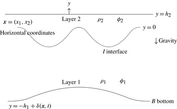
A two-layer model with a different, constant density in each layer is studied (figure 1). The interfacial motion is driven by gravity. Let
 $\boldsymbol{x}=(x_{1},x_{2})$
denote horizontal coordinates in the plane that coincides with the interface at rest,
 $y$
the vertical coordinate and
 $t$
the time. We denote the densities of the fluids by
 ${\it\rho}_{1}$
and
 ${\it\rho}_{2}$
, where index 1 refers to the lower layer and index 2 to the upper layer. Similarly, the layer depths at rest, far from any variation of the topography, are
 $h_{1}$
and
 $h_{2}$
, respectively. Let the position of the interface be determined by
 $y={\it\eta}(\boldsymbol{x},t)$
. Assuming incompressible and irrotational motion in each of the layers, the fluid motion is governed by the Laplacian potentials
 ${\it\phi}_{1}$
and
 ${\it\phi}_{2}$
. The values of the potentials along the interface are introduced as
 ${\it\phi}_{1I}(\boldsymbol{x},t)={\it\phi}_{1}(\boldsymbol{x},y={\it\eta},t)$
and
 ${\it\phi}_{2I}(\boldsymbol{x},t)={\it\phi}_{2}(\boldsymbol{x},y={\it\eta},t)$
, where indices
 $1I$
and
 $2I$
indicate that the potentials are evaluated on the lower and upper side of the interface, respectively, where
 $I$
denotes the interface. Using a set of differential equations, developed from the kinematic and dynamic boundary conditions at the interface, we integrate forward in time the interfacial elevation and the jump between the potentials at the interface, see § 3 below. Along the interface, the difference and sum of the potentials are introduced as
 $$\begin{eqnarray}{\it\Psi}(\boldsymbol{x},t)={\it\phi}_{1I}(\boldsymbol{x},t)-{\it\mu}{\it\phi}_{2I}(\boldsymbol{x},t),\quad {\it\Phi}(\boldsymbol{x},t)={\it\phi}_{1I}(\boldsymbol{x},t)+{\it\phi}_{2I}(\boldsymbol{x},t),\end{eqnarray}$$
where
 ${\it\mu}={\it\rho}_{2}/{\it\rho}_{1}$
denotes the density ratio of the fluids.
Sketch of the two-fluid model.

The upper boundary of fluid 2 is assumed to be horizontal, in the form of a rigid lid at
 $y=h_{2}$
. The lower fluid 1 has a bottom variation of
 $y=-h_{1}+{\it\delta}(\boldsymbol{x},t)$
. The function
 ${\it\delta}$
should be smooth, be of maximum (positive) height smaller than
 $h_{1}$
and decay to zero at infinity.
2.2. Integral equations
2.2.1. The potential in fluid 1
Solution of the Laplace equation is obtained using Green’s theorem. More specifically, for fluid 1, we apply Green’s theorem to the velocity potential
 ${\it\phi}_{1}(\boldsymbol{x},y)$
and a Green function. This is a three-dimensional source function given by
 $1/r$
, where
 $r=(R^{2}+(y^{\prime }-y)^{2})^{1/2}$
with
 $R=|(x_{1}^{\prime },x_{2}^{\prime })-(x_{1},x_{2})|$
denoting the horizontal distance. For convenience we apply
 $1/r+1/r_{1}$
as a Green function, where
 $1/r_{1}$
accounts for the image of
 $1/r$
with respect to
 $y=-h_{1}$
, i.e.
 $r_{1}=(R^{2}+(y^{\prime }+y+2h_{1})^{2})^{1/2}$
. Then
 $(\partial /\partial y)(1/r+1/r_{1})=0$
on
 $y=-h_{1}$
. Application of Green’s theorem to fluid 1 gives
 ${\it\phi}_{1}$
as
 $$\begin{eqnarray}\int _{S}\left[{\it\phi}_{1}^{\prime }\frac{\partial }{\partial n^{\prime }}\left(\frac{1}{r}+\frac{1}{r_{1}}\right)-\frac{\partial {\it\phi}_{1}^{\prime }}{\partial n^{\prime }}\left(\frac{1}{r}+\frac{1}{r_{1}}\right)\right]\!\text{d}S^{\prime }=-{\it\alpha}{\it\phi}_{1}(\boldsymbol{x},y),\end{eqnarray}$$
where the surface
 $S$
surrounds fluid 1, and where on the right-hand side
 ${\it\alpha}=2{\rm\pi}$
when the evaluation point
 $(\boldsymbol{x},y)$
is on the boundary
 $S$
and
 ${\it\alpha}=4{\rm\pi}$
when the evaluation point
 $(\boldsymbol{x},y)$
is inside fluid 1, see e.g. Newman (Reference Newman1977, p. 127). In (2.2)
 $n^{\prime }$
denotes the unit normal along the integration surface
 $S$
, pointing out of the fluid,
 $\text{d}S^{\prime }$
is a surface element, a prime indicates an integration variable and
 ${\it\phi}_{1}^{\prime }$
means
 ${\it\phi}_{1}(\boldsymbol{x}^{\prime },y^{\prime })$
, etc.
The surface
 $S$
surrounding fluid 1 includes the interface
 $I$
and bottom boundary
 $B$
, plus a vertical control surface
 $S_{c}$
in the far field. In our applications we assume that there is no motion at infinity, such that there is no contribution over
 $S_{c}$
in (2.2). It is possible to account for a constant background horizontal current where the integral over
 $S_{c}$
does not contribute. As a consequence, the surface integral in (2.2) is evaluated over the interface
 $I$
and bottom
 $B$
. For an evaluation point on the interface
 $I$
we obtain
 $$\begin{eqnarray}\int _{I+B}\left(\frac{1}{r}+\frac{1}{r_{1}}\right)\frac{\partial {\it\phi}_{1}^{\prime }}{\partial n^{\prime }}\text{d}S^{\prime }=2{\rm\pi}{\it\phi}_{1}+\int _{I+B}{\it\phi}_{1}^{\prime }\frac{\partial }{\partial n^{\prime }}\left(\frac{1}{r}+\frac{1}{r_{1}}\right)\!\text{d}S^{\prime },\quad (\boldsymbol{x},y={\it\eta})\text{ on }I.\end{eqnarray}$$
For an evaluation point on the bottom boundary
 $B$
an equation similar to (2.3) reads:
 $$\begin{eqnarray}2{\rm\pi}{\it\phi}_{1}=\int _{I+B}\left(\frac{1}{r}+\frac{1}{r_{1B}}\right)\frac{\partial {\it\phi}_{1}^{\prime }}{\partial n^{\prime }}\text{d}S^{\prime }-\int _{I+B}{\it\phi}_{1}^{\prime }\frac{\partial }{\partial n^{\prime }}\left(\frac{1}{r}+\frac{1}{r_{1B}}\right)\!\text{d}S^{\prime },\quad (\boldsymbol{x},y)\text{ on }B.\end{eqnarray}$$
In (2.4) the Green function is chosen as
 $1/r+1/r_{1B}$
, where
 $1/r_{1B}=(R^{2}+(y^{\prime }+y)^{2})^{-1/2}$
provides the image of
 $1/r$
with respect to
 $y=0$
such that
 $(\partial /\partial y)(1/r+1/r_{1B})=0$
on
 $y=0$
.
We employ
 ${\it\phi}_{1I}(\boldsymbol{x})={\it\phi}_{1}(\boldsymbol{x},y={\it\eta}(\boldsymbol{x}))$
along
 $I$
as introduced in the text above (2.1) and introduce
 ${\it\phi}_{1B}(\boldsymbol{x})={\it\phi}_{1}(\boldsymbol{x},y=-h_{1}+{\it\delta}(\boldsymbol{x}))$
along
 $B$
. Scaled normal velocities are introduced as
 $$\begin{eqnarray}V_{I}=\frac{\partial {\it\phi}_{1}}{\partial n}\sqrt{1+|\boldsymbol{{\rm\nabla}}_{H}{\it\eta}|^{2}}\quad \text{on }I,\quad V_{B}=\frac{\partial {\it\phi}_{1}}{\partial n}\sqrt{1+|\boldsymbol{{\rm\nabla}}_{H}{\it\delta}|^{2}}\quad \text{on }B.\end{eqnarray}$$
In (2.5)
 $\boldsymbol{{\rm\nabla}}_{H}=(\partial /\partial x_{1},\partial /\partial x_{2})$
denotes horizontal gradient;
 $\text{d}S=\sqrt{1+|\boldsymbol{{\rm\nabla}}_{H}{\it\eta}|^{2}}\text{d}x_{1}\text{d}x_{2}$
on
 $I$
and
 $\text{d}S=\sqrt{1+|\boldsymbol{{\rm\nabla}}_{H}{\it\delta}|^{2}}\text{d}x_{1}\text{d}x_{2}$
on
 $B$
.
2.2.2. Leading approximation of the integral equations for fluid 1
Successive approximations of the integral equations (2.3) and (2.4) are obtained by expanding the Green functions and their derivatives in
 ${\it\eta}$
and
 ${\it\delta}$
. For (2.3), using the expansions obtained in (A 1)–(A 4) in appendix A, the leading approximation of
 $1/r+1/r_{1}$
is given by
 $1/R+1/R_{1}$
in the integration over
 $I$
, and the leading approximation of
 $1/r+1/r_{1}$
is given by
 $2/R_{0}$
in the integration over
 $B$
. The leading approximation of the normal derivative of the Green function,
 $(\partial /\partial n^{\prime })(1/r+1/r_{1})$
, is given by
 $(\partial /\partial (2h_{1}))(1/R_{1})$
in the integration over
 $I$
, while this term is zero for the integration over
 $B$
. The leading approximation to (2.3) becomes
 $$\begin{eqnarray}\int \!\left(\frac{1}{R}+\frac{1}{R_{1}}\right)V_{I}^{\prime }\text{d}\boldsymbol{x}^{\prime }+\int \frac{2V_{B}^{\prime }}{R_{0}}\text{d}\boldsymbol{x}^{\prime }=2{\rm\pi}{\it\phi}_{1I}+\int {\it\phi}_{1I}^{\prime }\,\frac{\partial }{\partial (2h_{1})}\frac{1}{R_{1}}\text{d}\boldsymbol{x}^{\prime },\end{eqnarray}$$
where the integration is over the horizontal plane and
 $\text{d}\boldsymbol{x}^{\prime }=\text{d}x_{1}^{\prime }dx_{2}^{\prime }$
. The leading approximation to (2.4) is obtained similarly, using the expansions (A 5)–(A 8) in appendix A, giving
 $$\begin{eqnarray}2{\rm\pi}{\it\phi}_{1B}=\int \!\left(\frac{1}{R}+\frac{1}{R_{1}}\right)V_{B}^{\prime }\text{d}\boldsymbol{x}^{\prime }+\int \frac{2V_{I}^{\prime }}{R_{0}}\text{d}\boldsymbol{x}^{\prime }-\int {\it\phi}_{1B}^{\prime }\,\frac{\partial }{\partial (2h_{1})}\frac{1}{R_{1}}\text{d}\boldsymbol{x}^{\prime },\end{eqnarray}$$
where the integration is over the horizontal plane. Equations (2.6) and (2.7) are inverted by means of a Fourier transform. We employ the transform
 $(R^{2}+Y^{2})^{-1/2}=\mathscr{F}^{-1}[(2{\rm\pi}/k)\text{e}^{-\text{i}\boldsymbol{k}\boldsymbol{\cdot }\boldsymbol{x}^{\prime }-k|Y|}],|Y|\geqslant 0$
, where
 $\mathscr{F}$
denotes Fourier transform,
 $\mathscr{F}^{-1}$
inverse Fourier transform,
 $\boldsymbol{k}=(k_{1},k_{2})$
wavenumber and
 $k=|\boldsymbol{k}|$
. Taking the Fourier transform of (2.6) and (2.7) gives
 $$\begin{eqnarray}\displaystyle & \displaystyle \frac{1+\text{e}^{-2kh_{1}}}{k}\,\mathscr{F}(V_{I})+\frac{2\text{e}^{-kh_{1}}}{k}\,\mathscr{F}(V_{B})=\mathscr{F}({\it\phi}_{1I})-\text{e}^{-2kh_{1}}\mathscr{F}({\it\phi}_{1I}), & \displaystyle\end{eqnarray}$$
 $$\begin{eqnarray}\displaystyle & \displaystyle \mathscr{F}({\it\phi}_{1B})=\frac{1+\text{e}^{-2kh_{1}}}{k}\,\mathscr{F}(V_{B})+\frac{2\text{e}^{-kh_{1}}}{k}\,\mathscr{F}(V_{I})+\text{e}^{-2kh_{1}}\mathscr{F}({\it\phi}_{1B}). & \displaystyle\end{eqnarray}$$
 $V_{I}$
and
 ${\it\phi}_{1B}$
in terms of
 ${\it\phi}_{1I}$
and
 $V_{B}$
and are obtained in (2.10) and (2.12) below, respectively.
2.2.3. Successive approximations of
 $V_{I}$
and
${\it\phi}_{1B}$


The variable
 $V_{I}$
along
 $I$
and
 ${\it\phi}_{1B}$
along
 $B$
are obtained from the full integral equations (2.3) and (2.4) using the method of successive approximations (e.g. Mikhlin Reference Mikhlin1957). The variables are expanded as
 $V_{I}=V_{I}^{(1)}+V_{I}^{(2)}+V_{I}^{(3)}+\cdots \!\;$
and
 ${\it\phi}_{1B}={\it\phi}_{1B}^{(1)}+{\it\phi}_{1B}^{(2)}+{\it\phi}_{1B}^{(3)}+\cdots \,$
. The leading approximations to
 $V_{I}$
and
 ${\it\phi}_{1B}$
are given by
 $V_{I}^{(1)}$
and
 ${\it\phi}_{1B}^{(1)}$
, respectively, the quadratic approximations by
 $V_{I}^{(1)}+V_{I}^{(2)}$
and
 ${\it\phi}_{1B}^{(1)}+{\it\phi}_{1B}^{(2)}$
, and the cubic approximations by
 $V_{I}^{(1)}+V_{I}^{(2)}+V_{I}^{(3)}$
and
 ${\it\phi}_{1B}^{(1)}+{\it\phi}_{1B}^{(2)}+{\it\phi}_{1B}^{(3)}$
, etc. The contributions
 $V_{I}^{(1)},V_{I}^{(2)},V_{I}^{(3)},\dots$
and
 ${\it\phi}_{1B}^{(1)},{\it\phi}_{1B}^{(2)},\dots$
are obtained, respectively, from (2.3) with the Green function and its derivatives obtained from (A 1)–(A 4) in appendix A, and from (2.4) with the Green function and its derivatives obtained from (A 5)–(A 8), also in appendix A. After some algebra we obtain
 $$\begin{eqnarray}\displaystyle & \displaystyle \mathscr{F}(V_{I}^{(1)})=kT_{1}\mathscr{F}({\it\phi}_{1I})-\frac{\mathscr{F}(V_{B})}{C_{1}}, & \displaystyle\end{eqnarray}$$
 $$\begin{eqnarray}\displaystyle & \displaystyle \mathscr{F}(V_{I}^{(2)})=-kT_{1}\mathscr{F}({\it\eta}V_{I}^{(1)})-\text{i}\boldsymbol{k}\boldsymbol{\cdot }\mathscr{F}({\it\eta}\boldsymbol{{\rm\nabla}}_{H}{\it\phi}_{1I})+\frac{\text{i}\boldsymbol{k}\boldsymbol{\cdot }\mathscr{F}({\it\delta}\boldsymbol{{\rm\nabla}}_{H}{\it\phi}_{1B})}{C_{1}}, & \displaystyle\end{eqnarray}$$
 $T_{1}=\tanh (kh_{1})$
and
 $C_{1}=\cosh (kh_{1})$
are introduced. The contribution
 $V_{I}^{(3)}$
is obtained in (B 1)–(B 5) in appendix B.
For the potential
 ${\it\phi}_{1B}$
we obtain
 $$\begin{eqnarray}\displaystyle & \displaystyle \mathscr{F}({\it\phi}_{1B}^{(1)})=\frac{\mathscr{F}({\it\phi}_{1I})}{C_{1}}+\frac{T_{1}\,\mathscr{F}(V_{B})}{k}, & \displaystyle\end{eqnarray}$$
 $$\begin{eqnarray}\displaystyle & \displaystyle \mathscr{F}({\it\phi}_{1B}^{(2)})=-\frac{\mathscr{F}({\it\eta}V_{I}^{(1)})}{C_{1}}-\frac{T_{1}\,\text{i}\boldsymbol{k}}{k}\boldsymbol{\cdot }\mathscr{F}({\it\delta}\boldsymbol{{\rm\nabla}}_{H}{\it\phi}_{1B})-\mathscr{F}({\it\delta}V_{B}), & \displaystyle\end{eqnarray}$$
 ${\it\phi}_{1B}={\it\phi}_{1B}^{(1)}+{\it\phi}_{1B}^{(2)}$
.
2.2.4. The potential in fluid 2
The upper layer is bounded above by a rigid lid at
 $y=h_{2}$
. The motion in the upper layer is governed by the velocity potential
 ${\it\phi}_{2}(\boldsymbol{x},y)$
. A scaled normal velocity
 $W_{I}=(\partial {\it\phi}_{2}/\partial n)(1+|\boldsymbol{{\rm\nabla}}_{H}{\it\eta}|^{2})^{1/2}$
along
 $I$
, similar to
 $V_{I}$
in (2.5), is introduced, where the normal points into fluid 2. Expanding
 $W_{I}=W_{I}^{(1)}+W_{I}^{(2)}+W_{I}^{(3)}+\cdots \!\;$
we obtain
 $$\begin{eqnarray}\displaystyle & \mathscr{F}(W_{I}^{(1)})=-kT_{2}\mathscr{F}({\it\phi}_{2I}), & \displaystyle\end{eqnarray}$$
 $$\begin{eqnarray}\displaystyle & \mathscr{F}(W_{I}^{(2)})=kT_{2}({\it\eta}W_{I}^{(1)})-\text{i}\boldsymbol{k}\boldsymbol{\cdot }\mathscr{F}({\it\eta}\boldsymbol{{\rm\nabla}}_{H}{\it\phi}_{2I}), & \displaystyle\end{eqnarray}$$
 $T_{2}=\tanh (kh_{2})$
and
 ${\it\phi}_{2I}(\boldsymbol{x})={\it\phi}_{2}(\boldsymbol{x},y={\it\eta})$
along
 $I$
is used, as introduced in the text above (2.1). The variable
 $W_{I}^{(3)}$
is obtained in (B 6)–(B 9) (appendix B).
2.3. Evaluation of
${\it\Phi}={\it\phi}_{1I}+{\it\phi}_{2I}$
along the interface

While the difference potential
 ${\it\Psi}={\it\phi}_{1I}-{\it\mu}{\it\phi}_{2I}$
is integrated forward in time, see § 3 below, an equation for the sum potential
 ${\it\Phi}={\it\phi}_{1I}+{\it\phi}_{2I}$
is required in order to obtain
 ${\it\phi}_{1I}$
and
 ${\it\phi}_{2I}$
. Continuity of the normal velocity along the interface gives such an equation, i.e.
 $V_{I}=W_{I}$
. Using
 $V_{I}=V_{I}^{(1)}+V_{I}^{(2)}+V_{I}^{(3)}+\cdots \!\;$
and
 $W_{I}=W_{I}^{(1)}+W_{I}^{(2)}+W_{I}^{(3)}+\cdots \!\;$
we obtain
 $$\begin{eqnarray}\displaystyle 0 & = & \displaystyle \mathscr{F}(V_{I}-W_{I})=kT_{1}\mathscr{F}({\it\phi}_{1I})+kT_{2}\mathscr{F}({\it\phi}_{2I})-\frac{\mathscr{F}(V_{B})}{C_{1}}-\text{i}\boldsymbol{k}\boldsymbol{\cdot }\mathscr{F}({\it\eta}\boldsymbol{{\rm\nabla}}({\it\phi}_{1I}-{\it\phi}_{2I}))\nonumber\\ \displaystyle & & \displaystyle -\,kT_{1}\mathscr{F}\left[{\it\eta}\mathscr{F}^{-1}\left(kT_{1}\mathscr{F}({\it\phi}_{1I})-\frac{\mathscr{F}(V_{B})}{C_{1}}\right)\right]+\frac{\text{i}\boldsymbol{k}\boldsymbol{\cdot }\mathscr{F}({\it\delta}\boldsymbol{{\rm\nabla}}{\it\phi}_{1B})}{C_{1}}\nonumber\\ \displaystyle & & \displaystyle +\,kT_{2}\mathscr{F}[{\it\eta}\mathscr{F}^{-1}(kT_{2}\mathscr{F}({\it\phi}_{2I}))]+\mathscr{F}(V_{I}^{(3)}-W_{I}^{(3)})+\cdots \,.\end{eqnarray}$$
Introducing
 ${\it\phi}_{1I}=({\it\Psi}+{\it\mu}{\it\Phi})/(1+{\it\mu})$
and
 ${\it\phi}_{2I}=({\it\Phi}-{\it\Psi})/(1+{\it\mu})$
in (2.16) and multiplying the equation by
 $(1+{\it\mu})$
we obtain, successively,
 $$\begin{eqnarray}{\it\Phi}={\it\Phi}^{(1)}+{\it\Phi}^{(2)}+{\it\Phi}^{(3)}+\cdots \,,\end{eqnarray}$$
where the leading contribution is given by
 $$\begin{eqnarray}\mathscr{F}({\it\Phi}^{(1)})=\frac{T_{2}-T_{1}}{T_{2}+{\it\mu}T_{1}}\mathscr{F}({\it\Psi})+\frac{(1+{\it\mu})\,\mathscr{F}(V_{B})}{k(T_{2}+{\it\mu}T_{1})C_{1}},\end{eqnarray}$$
where
 $V_{B}$
is given in (2.5). An improved approximation is given by
 ${\it\Phi}^{(1)}+{\it\Phi}^{(2)}$
, where
 ${\it\Phi}^{(2)}$
accounts for quadratic coupling and is given by
 $$\begin{eqnarray}\mathscr{F}({\it\Phi}^{(2)})=\frac{\mathscr{F}(Q^{(2)})}{k(T_{2}+{\it\mu}T_{1})},\end{eqnarray}$$
where
 $$\begin{eqnarray}\displaystyle \mathscr{F}(Q^{(2)}) & = & \displaystyle kT_{1}\mathscr{F}[{\it\eta}\mathscr{F}^{-1}(kT_{1}\hat{{\it\Psi}})]+kT_{2}\mathscr{F}[{\it\eta}\mathscr{F}^{-1}(kT_{2}\hat{{\it\Psi}})]+2{\it\mu}\text{i}\boldsymbol{k}\boldsymbol{\cdot }\mathscr{F}({\it\eta}\boldsymbol{{\rm\nabla}}{\it\Psi})\nonumber\\ \displaystyle & & \displaystyle -\,\frac{\text{i}\boldsymbol{k}}{C_{1}}\boldsymbol{\cdot }\mathscr{F}\left[{\it\delta}\mathscr{F}^{-1}\left(\frac{\text{i}\boldsymbol{k}\hat{{\it\Psi}}}{C_{1}}\right)\right]-(1+{\it\mu})\left[kT_{1}\mathscr{F}\left[{\it\eta}\mathscr{F}^{-1}\left(\frac{\mathscr{F}(V_{B})}{C_{1}}\right)\right]\right.\nonumber\\ \displaystyle & & \displaystyle \left.+\,\frac{\text{i}\boldsymbol{k}}{C_{1}}\boldsymbol{\cdot }\mathscr{F}\left[{\it\delta}\mathscr{F}^{-1}\left(\frac{\text{i}\boldsymbol{k}}{k}T_{1}\mathscr{F}(V_{B})\right)\right]\right]\nonumber\\ \displaystyle & & \displaystyle +\,{\it\mu}kT_{1}\mathscr{F}[{\it\eta}\mathscr{F}^{-1}(kT_{1}\hat{{\it\Phi}})]-kT_{2}\mathscr{F}[{\it\eta}\mathscr{F}^{-1}(kT_{2}\hat{{\it\Phi}})]+({\it\mu}-1)\text{i}\boldsymbol{k}\boldsymbol{\cdot }\mathscr{F}({\it\eta}\boldsymbol{{\rm\nabla}}{\it\Phi})\nonumber\\ \displaystyle & & \displaystyle -\,\frac{{\it\mu}\text{i}\boldsymbol{k}}{C_{1}}\boldsymbol{\cdot }\mathscr{F}\left[{\it\delta}\mathscr{F}^{-1}\left(\frac{\text{i}\boldsymbol{k}\hat{{\it\Phi}}}{C_{1}}\right)\right],\end{eqnarray}$$
where on the right-hand side of (2.20)
 ${\it\Phi}={\it\Phi}^{(1)}+{\it\Phi}^{(2)}$
and the value of
 ${\it\Phi}^{(2)}$
is obtained iteratively. In (2.20) we have for simplicity set
 $\hat{{\it\Psi}}=\mathscr{F}({\it\Psi})$
and
 $\hat{{\it\Phi}}=\mathscr{F}({\it\Phi})$
. Terms including cubic couplings are obtained as
 $$\begin{eqnarray}\mathscr{F}({\it\Phi}^{(3)})=\frac{\mathscr{F}(Q^{(3)})}{k(T_{2}+{\it\mu}T_{1})},\end{eqnarray}$$
where
 $$\begin{eqnarray}\mathscr{F}(Q^{(3)})=-(1+{\it\mu})\left(\frac{\text{i}\boldsymbol{k}\boldsymbol{\cdot }\mathscr{F}({\it\delta}\boldsymbol{{\rm\nabla}}{\it\phi}_{1B}^{(2)})}{C_{1}}+\mathscr{F}(V_{I}^{(3)}-W_{I}^{(3)})\right)\!.\end{eqnarray}$$
The velocities
 $V_{I}^{(3)}$
and
 $W_{I}^{(3)}$
are given in (B 1) and (B 6) in appendix B, respectively, while
 ${\it\phi}_{1B}^{(2)}$
is given in (2.13).
3. Interfacial motion
3.1. Time integration
The kinematic boundary condition at the interface gives
 $$\begin{eqnarray}{\it\eta}_{t}-V_{I}=0\quad \text{at }I,\end{eqnarray}$$
where
 $V_{I}$
is given in (2.5). Alternatively,
 $W_{I}$
given in the text above (2.14) and (2.15) may be used. In the numerical implementation we use
 $(V_{I}+W_{I})/2$
in (3.1).
The pressure in each of the fluids is obtained from the Bernoulli equation, giving
 $p_{j}=-{\it\rho}_{j}[\partial {\it\phi}_{j}/\partial t+|\boldsymbol{v}_{j}|^{2}/2+gy]+\text{const.}$
, where
 $\boldsymbol{v}_{j}=\boldsymbol{{\rm\nabla}}{\it\phi}_{j}$
(
 $j=1,2$
) (note that we use
 $\boldsymbol{{\rm\nabla}}_{H}$
for the horizontal gradient). At the interface, the pressure is expressed in terms of
 ${\it\phi}_{jI}$
,
 $V_{I}$
and
 ${\it\eta}$
by (see Grue Reference Grue2002)
 $$\begin{eqnarray}p_{j}=-{\it\rho}_{j}\left[{\it\phi}_{jI,t}+g{\it\eta}+\frac{1}{2}\frac{|\boldsymbol{{\rm\nabla}}_{H}{\it\phi}_{jI}|^{2}-V_{I}^{2}-2V_{I}\boldsymbol{{\rm\nabla}}_{H}{\it\eta}\boldsymbol{\cdot }\boldsymbol{{\rm\nabla}}_{H}{\it\phi}_{jI}+|\boldsymbol{{\rm\nabla}}_{H}{\it\eta}\times \boldsymbol{{\rm\nabla}}_{H}{\it\phi}_{jI}|^{2}}{1+|\boldsymbol{{\rm\nabla}}_{H}{\it\eta}|^{2}}\right]+\text{const.},\end{eqnarray}$$
(
 $j=1,2$
). Continuity of the pressure at the interface gives, disregarding the effect of interface tension,
 $$\begin{eqnarray}\displaystyle ({\it\phi}_{1I}-{\it\mu}{\it\phi}_{2I})_{t}+g^{\prime }{\it\eta}=\mathscr{NL}_{2},\quad \text{at }I, & & \displaystyle\end{eqnarray}$$
 $$\begin{eqnarray}\displaystyle \mathscr{NL}_{2} & = & \displaystyle -\frac{|\boldsymbol{{\rm\nabla}}_{H}{\it\phi}_{1I}|^{2}-{\it\mu}|\boldsymbol{{\rm\nabla}}_{H}{\it\phi}_{2I}|^{2}-(1-{\it\mu})V_{I}^{2}}{2+2|\boldsymbol{{\rm\nabla}}_{H}{\it\eta}|^{2}}\nonumber\\ \displaystyle & & \displaystyle -\,\frac{-2V_{I}\boldsymbol{{\rm\nabla}}_{H}{\it\eta}\boldsymbol{\cdot }\boldsymbol{{\rm\nabla}}_{H}({\it\phi}_{1I}-{\it\mu}{\it\phi}_{2I})+|\boldsymbol{{\rm\nabla}}_{H}{\it\eta}\times \boldsymbol{{\rm\nabla}}_{H}{\it\phi}_{1I}|^{2}-{\it\mu}|\boldsymbol{{\rm\nabla}}_{H}{\it\eta}\times \boldsymbol{{\rm\nabla}}_{H}{\it\phi}_{2I}|^{2}}{2+2|\boldsymbol{{\rm\nabla}}_{H}{\it\eta}|^{2}},\nonumber\\ \displaystyle & & \displaystyle\end{eqnarray}$$
where in (3.3)
 $g^{\prime }=(1-{\it\mu})g$
denotes reduced gravity.
In the case of linear waves moving along a fluid of constant depth, i.e. the bottom of fluid 1 is located at
 $y=-h_{1}$
, the vertical velocities of the lower and upper fluid along the interface are given by
 $\mathscr{F}(V_{I}^{(1)})=kT_{1}\mathscr{F}({\it\phi}_{1I})$
and
 $\mathscr{F}(W_{I}^{(1)})=-kT_{2}\mathscr{F}({\it\phi}_{2I})$
, respectively, see the derivations in §§ 2.2.2–2.2.4; in particular (2.10) and (2.14), where in the former
 $V_{B}=0$
for a flat bottom. The sum gives
 $$\begin{eqnarray}\frac{\mathscr{F}(V_{I}^{(1)})}{kT_{1}}+\frac{{\it\mu}\mathscr{F}(W_{I}^{(1)})}{kT_{2}}=\mathscr{F}({\it\Psi})=\mathscr{F}({\it\phi}_{1I}-{\it\mu}{\it\phi}_{2I}),\end{eqnarray}$$
where the difference potential
 ${\it\Psi}$
is given in (2.1). A pseudo-vertical velocity
 $V_{I}^{(lin)}$
is defined, satisfying
 $$\begin{eqnarray}\left(\frac{1}{kT_{1}}+\frac{{\it\mu}}{kT_{2}}\right)\mathscr{F}(V_{I}^{(lin)})=\mathscr{F}({\it\Psi}),\end{eqnarray}$$
giving
 $\mathscr{F}(V_{I}^{(lin)})={\it\omega}^{2}\mathscr{F}({\it\Psi})/g^{\prime }$
, where
 ${\it\omega}^{2}$
is defined as
 $$\begin{eqnarray}{\it\omega}^{2}=\frac{g^{\prime }kT_{1}T_{2}}{T_{2}+{\it\mu}T_{1}}.\end{eqnarray}$$
Note that
 $V_{I}^{lin}$
differs from
 $V_{I}^{(1)}$
and
 $W_{I}^{(1)}$
, and further that
 ${\it\omega}^{2}$
appears through a definition from the analysis leading to (3.6). Equation (3.7) corresponds to the usual dispersion relation for linear interfacial waves in a two-layer fluid; this dispersion relation is real (no imaginary part). In the limit
 $kh_{1},kh_{2}\rightarrow 0$
we obtain
 $$\begin{eqnarray}c_{0}^{2}=\frac{{\it\omega}^{2}}{k^{2}}=\frac{g^{\prime }h_{1}h_{2}}{h_{2}+{\it\mu}h_{1}}.\end{eqnarray}$$
This defines the linear long-wave speed of the two-layer fluid.
The linear part of the prognostic equations is integrated analytically. This enhances the accuracy of the time integration such that a moderate time step can be used. Introducing dimensionless variables
 $\mathscr{F}({\it\Psi}^{\ast })=({\it\omega}/g^{\prime }h_{2})\mathscr{F}({\it\Psi})$
,
 ${\it\eta}^{\ast }={\it\eta}/h_{2}$
and
 $t^{\ast }=tc_{0}/h_{2}$
, the Fourier transforms of (3.1) and (3.3) become
 $$\begin{eqnarray}\displaystyle & \mathscr{F}({\it\eta}^{\ast })_{t^{\ast }}-{\it\omega}^{\ast }\mathscr{F}({\it\Psi}^{\ast })=\mathscr{F}(\mathscr{R}_{1}), & \displaystyle\end{eqnarray}$$
 $$\begin{eqnarray}\displaystyle & \mathscr{F}({\it\Psi}^{\ast })_{t^{\ast }}+{\it\omega}^{\ast }\mathscr{F}({\it\eta}^{\ast })=\mathscr{F}(\mathscr{R}_{2}), & \displaystyle\end{eqnarray}$$
 $\mathscr{F}(\mathscr{R}_{1})=\mathscr{F}(V_{I}-V_{I}^{(lin)})/c_{0}$
,
 $\mathscr{F}(\mathscr{R}_{2})=({\it\omega}c_{0}/g^{\prime })\mathscr{F}(\mathscr{NL}_{2}/c_{0}^{2})$
and
 $(\,)_{t^{\ast }}$
denotes time derivative.
 $V_{I},W_{I}$
are obtained successively from (2.10)–(2.11), (2.14)–(2.15) and (B 1), (B 6) in appendix B. The right-hand side
 $\mathscr{NL}_{2}$
is obtained from (3.4).
In
 $V_{I}^{(1)}$
, the contribution from
 $V_{B}$
, see (2.10), is obtained from the bottom boundary condition. In the case of a moving bottom we obtain
 $$\begin{eqnarray}{\it\delta}_{t}+V_{B}=0\quad \text{at }y=-h_{1}+{\it\delta}.\end{eqnarray}$$
In the special case when the bottom topography is moving with a horizontal velocity
 $\boldsymbol{U}(t)$
we obtain
 ${\it\delta}_{t}=-\boldsymbol{U}(t)\boldsymbol{\cdot }\boldsymbol{{\rm\nabla}}_{H}{\it\delta}$
, giving
 $V_{B}=\boldsymbol{U}(t)\boldsymbol{\cdot }\boldsymbol{{\rm\nabla}}_{H}{\it\delta}$
. For a rigid, non-moving bottom,
 $V_{B}=0$
.
Regarding initial conditions, the fluid and bottom velocities are zero at
 $t=0$
in the present applications, except for the time stepping of the solitary waves in § 4.2 below, where the wave motion and potentials in the constant depth case are specified at
 $t=0$
.
3.1.1. Other forcing mechanisms. Coriolis force
Forcing mechanisms other than moving the bottom geometry are possible, e.g. prescribing a pressure at the upper boundary. However, that would imply a reformulation of the kinematic (and dynamic) boundary conditions at the upper boundary.
Wave diffraction of a slowly rotating geometry, accounting for the effect of the non-Newtonian Coriolis force, has been formulated via potential theory by Grue & Palm (Reference Grue and Palm1996). The perturbation analysis developed in the frequency domain was performed for a single-layer fluid and may be extended to the two-layer case. The present time integration formulation may not be directly suitable for including the effect of the Coriolis force. A problem is connected to the periodic extensions at the boundaries of the horizontal computational domain.
Thus, the present model and simulations of a field experiment, see § 6, do not take into account rotational effects, which are present in any realistic oceanic setting, particularly at high latitudes. While the wave generation during a short time frame, using the present method, may be realistic, the subsequent wave evolution is modified by rotational effects, where an additional term appears in the dispersion relation (e.g. Grimshaw & Helfrich Reference Grimshaw and Helfrich2012, their equation (6)). See also Ostrovsky (Reference Ostrovsky1978). Such an additional rotational correction is not accounted for in the dispersion relation in the present model, see (3.7).
3.2. Numerical implementation
Equations (3.9)–(3.10) in matrix form read
 $\mathscr{F}(Y)_{t}+\unicode[STIX]{x1D63C}\mathscr{F}(Y)=\mathscr{F}(\mathscr{R})$
, where
 $Y=[{\it\eta},{\it\Psi}]^{\text{T}}$
,
 $\mathscr{R}=[\mathscr{R}_{1},\mathscr{R}_{2}]^{\text{T}}$
, with
 $[\,]^{\text{T}}$
denoting transpose. The symbols with stars are omitted in what follows. The matrix
 $\unicode[STIX]{x1D63C}$
and its variant
 $\text{e}^{\unicode[STIX]{x1D63C}(t-t_{0})}$
are given by
 $$\begin{eqnarray}\unicode[STIX]{x1D63C}=\left[\begin{array}{@{}cc@{}}0 & -{\it\omega}\\ {\it\omega} & 0\end{array}\right],\quad \text{e}^{\unicode[STIX]{x1D63C}(t-t_{0})}=\left[\begin{array}{@{}cc@{}}\cos {\it\omega}(t-t_{0}) & -\!\sin {\it\omega}(t-t_{0})\\ \sin {\it\omega}(t-t_{0}) & \cos {\it\omega}(t-t_{0})\end{array}\right].\end{eqnarray}$$
The equation
 $$\begin{eqnarray}\mathscr{F}(Z)_{t}=\text{e}^{\unicode[STIX]{x1D63C}(t-t_{0})}\mathscr{F}(\mathscr{R})\end{eqnarray}$$
is integrated forward in time using a fourth-order Runge–Kutta scheme with a constant time step, where
 $$\begin{eqnarray}\mathscr{F}(Y)=\text{e}^{-\unicode[STIX]{x1D63C}(t-t_{0})}\mathscr{F}(Z)\end{eqnarray}$$
provides the relation between the
 $Y$
-variable and the auxiliary
 $Z$
-variable, obtained by integrating (3.13). In (3.13) and (3.14)
 $t_{0}$
means the time of the previous time step, or the starting time of the time integration. At each time step the variables
 ${\it\eta}$
and
 ${\it\Psi}$
are used as input to obtain
 ${\it\Phi}$
, whereby the potentials
 ${\it\phi}_{1I}$
and
 ${\it\phi}_{2I}$
are evaluated. The velocities
 $V_{I}$
,
 $W_{I}$
and the right-hand side
 $\mathscr{R}=[\mathscr{R}_{1},\mathscr{R}_{2}]^{\text{T}}$
are then obtained. The time integration using (3.13) yields the linear part analytically, implying that the relatively small nonlinear terms on the right-hand side can be dealt with using a relatively moderate time step.
The method is used for two- and three-dimensional calculations. In the two-dimensional implementation, a wave tank of length
 $L_{1}$
has
 $N_{1}$
nodes, giving
 ${\rm\Delta}x_{1}=L_{1}/N_{1}$
. The wavenumber vector in spectral space reads
 $(\!0,{\rm\Delta}k_{1},2{\rm\Delta}k_{1},\dots ,$
 $(N_{1}/2-1){\rm\Delta}k_{1},-(N_{1}/2){\rm\Delta}k_{1},\dots ,-{\rm\Delta}k_{1}\! )$
, where
 ${\rm\Delta}k_{1}=2{\rm\pi}/L_{1}$
. A MATLAB script with MATLAB FFT routines is used in the two-dimensional calculations. The three-dimensional calculations, using a Fortran code (§§ 5 and 6 below), employ a rectangular wave tank of length
 $L_{1}$
and width
 $L_{2}$
, discretized with
 $N_{1}\times N_{2}$
nodes, with
 $({\rm\Delta}x_{1},{\rm\Delta}x_{2})=(L_{1}/N_{1},L_{2}/N_{2})$
and
 $({\rm\Delta}k_{1},{\rm\Delta}k_{2})=(2{\rm\pi}/L_{1},2{\rm\pi}/L_{2})$
. Each product between two physical variables is transformed to Fourier space, where the upper half of the spectrum is set to zero (zero-padding). The result is then transformed back into the physical space. No smoothing is applied. The number of operations in the method is governed by the number of FFT operations, which is
 $O(N_{0}\log N_{0})$
, where
 $N_{0}=N_{1}\times N_{2}$
is the number of nodes in the calculations. Further comments on the calculation procedures and efficiency are given in § 4.3 below.
4. Numerical experiments in two dimensions
4.1. Numerical calculations of
${\it\Phi}$

The accuracy and convergence of the successive approximations of the potential
 ${\it\Phi}$
obtained in (2.17) (see § 2.3) are investigated through numerical examples. First we perform a set of computations of interfacial solitary waves of finite, moderate and large amplitude. Available reference solutions using the fully nonlinear and dispersive method documented in Grue et al. (Reference Grue, Jensen, Rusås and Sveen1999) give
 ${\it\Psi}={\it\phi}_{1I}-{\it\mu}{\it\phi}_{2I}$
and the elevation
 ${\it\eta}$
. These are used as input to the calculations of the various approximations of
 ${\it\Phi}$
. The bottom of fluid 1 is at
 $y_{1}=-h_{1}$
.
Solitary depression waves of amplitude up to twice the upper layer depth for
 $h_{1}/h_{2}=6$
and
 $1-{\it\rho}_{2}/{\it\rho}_{1}\ll 1$
are obtained (
 $|x_{1}|<100h_{2},N_{1}=400$
). Calculations using the quadratic approximation
 ${\it\Phi}\simeq {\it\Phi}^{(1)}+{\it\Phi}^{(2)}$
, with
 ${\it\Phi}^{(1)}$
obtained from (2.18) and
 ${\it\Phi}^{(2)}$
from (2.19) and (2.20), fit to the fully nonlinear reference solution, within graphical accuracy, for the solitary wave amplitudes
 $a_{0}/h_{2}$
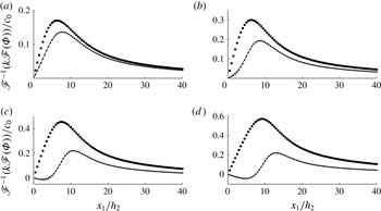
of 0.5, 1, 1.6 and 2. This illustrates the rapid convergence of the successive approximations employed in the calculations. The results in figure 2 are shown for
 $x_{1}$
-values between 0 and
 $40h_{2}$
, where
 $x_{1}=0$
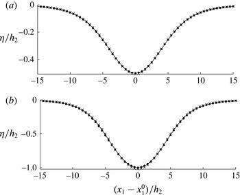
refers to the point of maximum amplitude of the solitary waves. Interfacial profiles are visualized in figure 4 for
 $a_{0}/h_{2}=0.5$
and 1. Calculations using only
 ${\it\Phi}^{(1)}$
, obtained from (2.18), give results quite far from the exact solution, even for the moderately small amplitude of
 $a_{0}/h_{2}=0.5$
. The difference between
 ${\it\Phi}^{(1)}$
and the numerically exact
 ${\it\Phi}$
increases with increasing amplitude, becoming very large when
 $a_{0}/h_{2}=2$
(figure 2
d).
Calculation of the potential
 $\mathscr{F}^{-1}(k\mathscr{F}({\it\Phi}))/c_{0}=\mathscr{F}^{-1}(k\mathscr{F}({\it\phi}_{1I}+{\it\phi}_{2I}))/c_{0}$
for solitary depression waves of amplitude
 $a_{0}$
. Elevation
 ${\it\eta}$
and
 ${\it\phi}_{1}-{\it\mu}{\it\phi}_{2}$
given as input.
 ${\it\Phi}^{(1)}$
obtained from (2.18) (⚫),
 ${\it\Phi}^{(1)}+{\it\Phi}^{(2)}$
with
 ${\it\Phi}^{(2)}$
obtained from (2.19) to (2.20) (●), fully nonlinear (exact) reference computation (——). (a)
 $a_{0}/h_{2}=0.5$
; (b)
 $a_{0}/h_{2}=1$
; (c)
 $a_{0}/h_{2}=1.6$
; (d)
 $a_{0}/h_{2}=2$
.
 $h_{1}/h_{2}=6$
,
 ${\it\mu}=1$
.
 ${\rm\Delta}x_{1}/h_{2}=0.5$
.

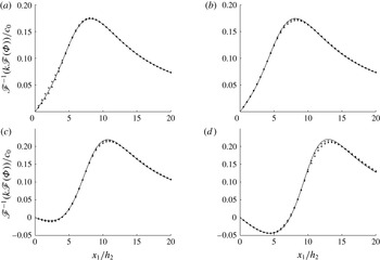
The convergence of the successive approximations is further explored by comparing numerical values of
 ${\it\Phi}^{(1)}+{\it\Phi}^{(2)}$
and
 ${\it\Phi}^{(1)}+{\it\Phi}^{(2)}+{\it\Phi}^{(3)}$
. In figure 3(a) the two approximations are compared for
 $a_{0}/h_{2}=0.8$
, which is a typical amplitude of the time simulations performed below. Both
 ${\it\Phi}^{(1)}+{\it\Phi}^{(2)}$
and
 ${\it\Phi}^{(1)}+{\it\Phi}^{(2)}+{\it\Phi}^{(3)}$
are very close to the reference solution, which means that
 ${\it\Phi}^{(3)}$
is very small. Only a small part of the computational domain, from the point of maximal depression at
 $x_{1}=0$
to
 $x_{1}/h_{2}=20$
, is visualized.
Same as figure 2. Quadratic (●), cubic (
 $+$
), fully nonlinear (exact) (——). (a)
 $a_{0}/h_{2}=0.8$
,
 $h_{0}=0$
; (b)
 $a_{0}/h_{2}=0.8$
,
 $h_{0}/h_{2}=1$
; (c)
 $a_{0}/h_{2}=1.6$
,
 $h_{0}/h_{2}=1$
;(d)
 $a_{0}/h_{2}=2$
,
 $h_{0}/h_{2}=1.5$
.
 $h_{1}/h_{2}=6$
,
 ${\it\mu}=1$
,
 ${\rm\Delta}x_{1}/h_{2}=0.5$
.

We also calculate the solitary waves with another reference depth of the layers, with a modified upper layer depth of
 $\tilde{h}_{2}=h_{2}+h_{0}$
, lower layer depth of
 $\tilde{h}_{1}=h_{1}-h_{0}$
and elevation of
 $\tilde{{\it\eta}}={\it\eta}+h_{0}$
. The calculations further illustrate the contributions from the quadratic and cubic approximations. The results for the same solitary wave amplitude of
 $a_{0}/h_{2}=0.8$
, with
 $h_{0}/h_{2}=1$
, show that
 ${\it\Phi}^{(1)}+{\it\Phi}^{(2)}+{\it\Phi}^{(3)}$
now compares somewhat better than
 ${\it\Phi}^{(1)}+{\it\Phi}^{(2)}$
to the reference at the peak value of
 $\mathscr{F}^{-1}(k\mathscr{F}({\it\Phi}))/c_{0}$
at
 $x_{1}/h_{2}\sim 7{-}8$
(figure 3
b) (where
 $c_{0}$
is defined in (3.8)). The difference between the approximations is extremely small for the other
 $x_{1}$
-values. The same convergence and small difference between the approximations and the reference solution are obtained also for the amplitudes of
 $a_{0}/h_{2}=1.6$
and 2, see figure 3(c,d). Calculations of solitary waves of very large amplitude, for a layer depth of
 $h_{1}/h_{2}=20.4$
, show that the quadratic approximation
 $V_{I}^{(1)}+V_{I}^{(2)}$
is excellent for amplitudes even as large as
 $a_{0}/h_{2}=5$
. Similar calculations of
 $W_{I}^{(1)}+W_{I}^{(2)}$
are also excellent (Grue Reference Grue2013b
).
Two important conclusions can be drawn from the calculations in this subsection:
-
(i)
${\it\Phi}$
obtained from the quadratic approximation
${\it\Phi}^{(1)}+{\it\Phi}^{(2)}$
provides a very accurate evaluation of the sum potential for solitary waves of amplitude
$a_{0}/h_{2}=O(1)$
, when compared to the fully nonlinear reference solution. This is the relevant range of amplitudes for the time simulations of waves generated at a three-dimensional topography. (For comparison to approximations using the KdV equation, see § 4.4.) -
(ii) Calculations including the cubic approximation show that
${\it\Phi}^{(3)}$
is much smaller than
${\it\Phi}^{(1)}+{\it\Phi}^{(2)}$
and illustrate the rapid convergence and usefulness of the successive approximations in the interfacial wave calculations.


4.2. Time simulations in two dimensions
Time integration of solitary wave propagation during
 $2\times 10^{4}$
time steps of
 ${\rm\Delta}tc_{0}/h_{2}=0.005$
shows that the quadratic and cubic approximations compare excellently to the fully nonlinear solution (Grue et al.
Reference Grue, Jensen, Rusås and Sveen1999), for amplitudes of
 $a_{0}/h_{2}=0.5$
and 1, depth ratio
 $h_{1}/h_{2}=6$
and density ratio
 $1-{\it\rho}_{2}/{\it\rho}_{1}\ll 1$
(table 1, figure 4).
Time stepping of solitary waves of amplitude
 $a_{0}/h_{2}=0.5$
and 1, using fully nonlinear (FNL) (Grue et al.
Reference Grue, Jensen, Rusås and Sveen1999), quadratic and cubic calculations with time step
 ${\rm\Delta}tc_{0}/h_{2}=0.005$
.

Solitary waves of depression integrated forward a distance
 $x_{0}$
. Quadratic approximation (
 $\times$
), cubic approximation (●), reference (——). (a) Amplitude
 $a_{0}/h_{2}=0.5$
,
 $x_{1}^{0}/h_{2}=117$
, number of time steps: 20 030 (quadratic); 20 036 (cubic). (b) Amplitude
 $a_{0}/h_{2}=1$
,
 $x_{1}^{0}/h_{2}=129$
, number of time steps: 20 054 (quadratic); 20 065 (cubic).
 ${\rm\Delta}x_{1}/h_{2}=0.5$
,
 ${\rm\Delta}tc_{0}/h_{2}=0.005$
,
 $h_{1}/h_{2}=6$
,
 ${\it\rho}_{2}/{\it\rho}_{1}=1$
.

The interfacial motion driven by an oscillating two-dimensional bump on the bottom is shown in figure 5. The bottom topography has shape
 ${\it\delta}(\boldsymbol{x},t)=d_{m}(1+\tanh ((x_{1}-x_{1}^{a})/3.5h_{2}))(1+\tanh ((x_{1}^{b}-x_{1})/3.5h_{2}))/4$
, where
 $d_{m}$
denotes the maximum height and
 $x_{1}^{b}-x_{1}^{a}=34h_{2}$
. The bottom topography is moved in a sinusoidal manner with a horizontal velocity of
 $U(t)=U_{m}\sin {\it\Omega}t$
, starting from rest. The figure shows the formation of interfacial waves after time
 ${\it\Omega}t=3{\rm\pi}/2$
, corresponding to three-quarters of a total period of oscillation. The value of
 ${\it\Omega}h_{2}/c_{0}$
is
 $1/70$
, relevant to the three-dimensional calculations in §§ 5 and 6 below. Two different topography heights
 $d_{m}$
, two different layer depths and two different Froude numbers (0.5 and 0.7) are tested. The interfacial wave trains attain a local wave height comparable to the upper layer depth
 $h_{2}$
. The results in figure 5 show that both the quadratic and cubic approximations give an excellent representation of the wave generation due to oscillatory motion of the topography. The rapid convergence and usefulness of the successive approximations are illustrated. In figure 5 we have also included calculations using the linear approximation, where no nonlinear coupling terms are included, giving numerical solutions with no wave formation.
Elevation
 ${\it\eta}$
at
 $t=(3{\rm\pi}/2)/{\it\Omega}$
with cubic (——), quadratic (●) and linear approximation (◼) driven by a moving bottom topography for (a)
 $U_{0}/c_{0}=0.7$
,
 $h_{1}=4h_{2}$
,
 $d_{m}/h_{2}=1$
; (b)
 $U_{0}/c_{0}=0.5$
,
 $h_{1}=6h_{2}$
,
 $d_{m}/h_{2}=2.5$
. Motion of bottom topography:
 $U(t)=U_{0}\sin {\it\Omega}t$
,
 ${\it\Omega}h_{2}/c_{0}=1/70$
,
 ${\it\rho}_{2}/{\it\rho}_{1}=1$
. RK4 with
 ${\rm\Delta}tc_{0}/h_{2}=0.0825$
, 4000 time steps,
 $L=600$
,
 $N=1000$
. Bottom shape:
 ${\it\delta}(x_{1},t)=d_{m}((1/2)+(\tanh ((x_{1}-x_{1}^{a})/3.5h_{2}))/2)((1/2)+(\tanh ((x_{1}^{b}-x_{1})/3.5h_{2}))/2)$
. Initially,
 $x_{1}^{a}=100h_{2}$
,
 $x_{1}^{b}=134h_{2}$
.

4.3. Comments on the calculation procedures and efficiency
The results illustrate the accuracy of the quadratic and cubic approximations in obtaining interfacial waves with amplitudes up to unity. Moreover, the differences between the quadratic and cubic calculations are very small. Use of the quadratic approximation requires fewer products and temporal variables than the cubic approximation. This is beneficial in the three-dimensional calculations, where the available RAM represents a practical limitation on the maximum number of variables. In the three-dimensional version of the method implemented in Fortran we employ the quadratic approximation using
 ${\it\Phi}\simeq {\it\Phi}^{(1)}+{\it\Phi}^{(2)}$
,
 $V_{I}\simeq V_{I}^{(1)}+V_{I}^{(2)}$
and
 $W_{I}\simeq W_{I}^{(1)}+W_{I}^{(2)}$
. With the streamlined Fortran code we employ
 $N_{0}=720\times 720\simeq 0.5\times 10^{6}$
calculation nodes in the horizontal plane on a Lenovo T430 Thinkpad. Calculations using
 $720\times 720$
and
 $500\times 500$
nodes take 6 and 2.2 s per time step, respectively, confirming the computational demands are
 $O(N_{0}\log N_{0})$
, as mentioned at the end of § 3.2.
We note that, for surface waves, Fructus et al. (Reference Fructus, Clamond, Grue and Kristiansen2005a
) have fully tested the numerical implementation of the cubic version, including the full representation of the remaining integrals appearing in the exact integral equation formulation, where the remaining integrals decay rapidly in space, implying only local integration of these integrals is required rather than evaluation over the entire horizontal plane. Moreover, Clamond, Fructus & Grue (Reference Clamond, Fructus and Grue2007) tested time integrators, varying the time step – with the accuracy depending on the local nonlinearity – also for surface waves. Three-dimensional surface wave patterns were obtained by Fructus et al. (Reference Fructus, Kharif, Francius, Kristiansen, Clamond and Grue2005b
) using up to
 $N_{0}=10^{4}$
nodes, much smaller than the present three-dimensional interfacial calculations using
 $N_{0}=0.5\times 10^{6}$
nodes.
4.4. Comparison to the KdV equation
The present method is fully dispersive, as it resolves the entire wavenumber spectrum up to the truncation. While the variables are represented along the exact position of the interface and bottom variation, accounting thus for an important part of the nonlinearity, the integral equations giving
 $V_{I}$
and
 $W_{I}$
along
 $I$
and
 ${\it\phi}_{1B}$
along
 $B$
are approximated, here retaining the quadratic and cubic approximations. The method differs fundamentally from the KdV equation or its extensions, where the KdV equation is valid in the long-wave range. Specifically, interfacial KdV solitons (
 $\text{sech}^{2}$
-profiles) differ fundamentally from the fully nonlinear interfacial waves when the amplitude exceeds 0.4 times the thinner layer depth, as visualized by Grue et al. (Reference Grue, Jensen, Rusås and Sveen1999). For surface waves, the present method and the KdV equation have been used to calculate fission of the 2004 Indian Ocean tsunami in the shallow Strait of Malacca, finding that the KdV equation has limited capacity in resolving dispersion in comparison with the fully dispersive method (Grue et al.
Reference Grue, Pelinovsky, Fructus, Kharif and Talipova2008). For interfacial solitary waves, the KdV equation is found to be valid up to a wave amplitude of
 $a/h_{2}=0.4$
(Grue et al.
Reference Grue, Jensen, Rusås and Sveen1999). The two-dimensional, fully nonlinear interfacial calculations of Grue et al. (Reference Grue, Friis, Palm and Rusås1997) obtained very good agreement with laboratory experiments on unsteady transcritical two-layer flow over a bottom topography, where bad agreement with weakly nonlinear interfacial KdV theories was reported (Melville & Helfrich Reference Melville and Helfrich1987).
4.5. Comments on the Kelvin–Helmholtz instability
Experiments on shear-induced breaking in strongly nonlinear solitary waves show that the most unstable wavelength is 6–8 times the thickness of a thin pycnocline, with depth ratio
 $h_{1}/h_{2}\simeq 5$
and
 ${\rm\Delta}h/h_{2}\simeq 1/4$
(Fructus et al.
Reference Fructus, Carr, Grue, Jensen and Davies2009, table 1). In the present interfacial calculations, where the most unstable wavelength is even shorter, values of
 ${\rm\Delta}x_{1}/h_{2}$
are in the range above 0.5. The maximum wavenumber of
 $2{\rm\pi}(N/4)/L_{1}$
(the energy for higher wavenumbers is padded to zero) corresponding to a shortest wavelength of
 $4{\rm\Delta}x_{1}>2h_{2}$
does not resolve the length scale of the Kelvin–Helmholtz instability in the present calculations. A different instability occurs during strong interfacial interactions with a shallow geometry, in the form of a collapse, overturning and subsequent mixing of the thin pycnocline, see Sveen et al. (Reference Sveen, Guo, Davies and Grue2002, figure 6). This kind of instability is observed in the three-dimensional calculations for very strong forcing, where the interface touches the top of the bottom geometry (results not shown).
5. Comparison to laboratory experiments
The three-dimensional method using the quadratic approximation is used to simulate a set of laboratory experiments carried out by Maxworthy (Reference Maxworthy1979). He investigated the generation of trains of solitary waves due to the barotropic tidal flow of a stratified fluid over a three-dimensional bottom topography. The experiments were performed in a square wave tank of side 245 cm filled with a fluid layer of depth 10 cm. The fluid layer had a stratification near the bottom, with a pycnocline centred around a level of approximately 0.6 cm above the bottom. We shall take the mid-level of the pycnocline at 0.6 cm as the reference depth and the length scale (
 $h_{2}$
) in the computations. Topography in the form of a ridge with a horizontal rectangular top, 16 cm wide and 60 cm long, was applied in the experiments. The ridge had constant slopes to the sides, forming another rectangle of
 $30~\text{cm}\times 76~\text{cm}$
at the base. The geometry was towed horizontally upside down in the top part of the fluid layer, driving the wave motion along the pycnocline. The time-varying speed
 $U(t)=U_{m}\sin {\it\Omega}t$
of the ridge was along the direction of its width (the
 $x_{1}$
-direction), where
 $U_{m}$
denotes the maximum speed and
 $2{\rm\pi}/{\it\Omega}$
the cyclic (tidal) period. Upstream wave formation was investigated varying the Froude number
 $\mathit{Fr}=U_{m}/c_{0}$
(
 $c_{0}$
defined in (3.8)) and the non-dimensional ridge height
 $d_{m}/H$
, where
 $H=h_{1}+h_{2}$
.
The layer depths of the two-fluid system, size of wave tank, shape and motion of the topography in the calculations are similar to those in the laboratory experiments. With
 $H=h_{1}+h_{2}=10$
cm and
 $h_{2}\simeq 0.6$
cm as reference depth, the depth ratio becomes
 $h_{1}/h_{2}=15.6$
. The length of the wave tank of 245 cm becomes
 $408h_{2}$
. The theoretical topography has width and length at the half-height of
 $20.4~\text{cm}\simeq 34h_{2}$
and
 $67~\text{cm}\simeq 112h_{2}$
, respectively. The shape of the topography used in the computations is given by
 ${\it\delta}(x_{1},x_{2})=d_{m}f_{1}(x_{1})f_{2}(x_{2})$
, where
 $d_{m}$
denotes the maximum height and
 $$\begin{eqnarray}\displaystyle & f_{1}(x_{1})={\textstyle \frac{1}{4}}[1+\tanh ((x_{1}-x_{1}^{a})/3.5h_{2})][1-\tanh ((x_{1}-x_{1}^{b})/3.5h_{2})], & \displaystyle\end{eqnarray}$$
 $$\begin{eqnarray}\displaystyle & f_{2}(x_{2})={\textstyle \frac{1}{4}}[1+\tanh ((x_{2}-x_{2}^{c})/3.5h_{2})][1-\tanh ((x_{2}-x_{2}^{d})/3.5h_{2})], & \displaystyle\end{eqnarray}$$
 $x_{1}^{b}-x_{1}^{a}=34h_{2}$
and
 $x_{2}^{d}-x_{2}^{c}=112h_{2}$
. The excursion of the ridge after a half-period, corresponding to
 $2U_{m}/{\it\Omega}$
, can be estimated from the experimental results. The velocity
 $U_{m}$
is obtained from the Froude number
 $\mathit{Fr}=U_{m}/c_{0}$
, which is given in the experiments. The experimental density stratification is used to estimate
 $c_{0}$
. In non-dimensional terms,
 ${\it\Omega}h_{2}/c_{0}\simeq 1/70$
can be estimated from the experiments and is used in the simulations. The numerical wave tank extends horizontally
 $400h_{2}$
by
 $400h_{2}$
, with 500 nodes in each direction (
 ${\rm\Delta}x_{1}={\rm\Delta}x_{2}=0.8h_{2}$
). The topography is moved according to
 $U(t)/c_{0}=\mathit{Fr}\sin {\it\Omega}t$
for
 ${\it\Omega}t$
between 0 and
 ${\rm\pi}$
, and is stopped for
 ${\it\Omega}t>{\rm\pi}$
. The time step is
 ${\rm\Delta}t=0.22h_{2}/c_{0}$
.
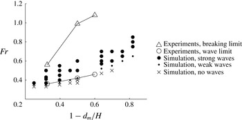
Maxworthy plotted his experimental results for the occurrence of the wave formation in the
 $(1-d_{m}/H,\mathit{Fr})$
-plane. Waves occurred when
 $\mathit{Fr}$
exceeded the straight line between the points
 $(1-d_{m}/H,\mathit{Fr})=(0.33,0.36)$
and
 $(1-d_{m}/H,\mathit{Fr})=(0.6,0.46)$
, with experimental error bars of
 $\mathit{Fr}=\pm 0.025$
(Maxworthy Reference Maxworthy1979, figure 6). The experimental transition line is indicated in the present figure 6. He also investigated the occurrence of wave breaking, also indicated in the figure.
Comparison between experiments carried out by Maxworthy (Reference Maxworthy1979) and numerical simulations using the present method, on the occurrence of internal waves in a layered fluid driven by a sinusoidally oscillating bottom topography as a function of the bottom topography height
 $d_{m}$
and Froude number
 $\mathit{Fr}=U_{0}/c_{0}$
. Depth ratio
 $h_{1}/h_{2}=15.6$
.
 ${\it\Omega}h_{2}/c_{0}=1/70$
.
 $H=h_{1}+h_{2}$
. Experimental wave limit (○) and breaking limit ( △ ). Computational strong waves with amplitude
 $O(h_{2})$
(⚫); weak waves with wave height
 ${\sim}0.2h_{2}$
(●; see the definition in the main text); no waves (
 $\times$
).

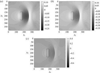
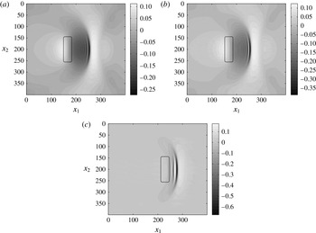
Weak wave formation appears in the computations when a certain value of the Froude number is exceeded, corresponding exactly to the experiments carried out by Maxworthy (figure 6). His transition line for the onset of wave formation is further explored and extended here. Two calculated examples of weak wave trains at half-period (
 ${\it\Omega}t={\rm\pi}$
), both with leading trough-to-crest height of
 $0.2h_{2}$
, for a small Froude number of
 $\mathit{Fr}=0.35$
in both cases, are shown in figures 7(a) and 8(a), for
 $1-d_{m}/H=0.32$
and 0.25, respectively. The leading trough-to-crest height almost doubles for the somewhat stronger
 $\mathit{Fr}=0.37$
(figures 7
b, 8
b) and becomes comparable to the layer depth
 $h_{2}$
for the even stronger
 $\mathit{Fr}=0.41$
(figure 7
c). Appreciable wave height occurs for the much larger Froude number of
 $\mathit{Fr}=0.8$
when the height
 $d_{m}/H$
is small (figure 8
c). Occurrences of weak wave trains (of wave height
 ${\sim}0.2h_{2}$
) for other values of
 $\mathit{Fr}$
and
 $d_{m}$
are indicated by the small dots in figure 6. Simulations with too small a Froude number or too small a topography height show no formation of a wave train, as indicated by the crosses in the figure. The present two-layer simulations with 40 different combinations of
 $0.25<1-d_{m}/H<0.82$
and
 $0.33<\mathit{Fr}<0.85$
confirm and extend the threshold of the wave formation as found experimentally by Maxworthy.
Interfacial elevation
 ${\it\eta}/h_{2}$
at
 ${\it\Omega}t={\rm\pi}$
(half-period) for
 $1-d_{m}/H=0.32$
. (a)
 $\mathit{Fr}=0.35$
, (b)
 $\mathit{Fr}=0.37$
, (c)
 $\mathit{Fr}=0.41$
.
 ${\it\Omega}h_{2}/c_{0}=1/70$
. Same resolution and shape of the geometry as in figure 6. Position of geometry, at half-height, at
 ${\it\Omega}t={\rm\pi}$
, indicated.

Interfacial elevation
 ${\it\eta}/h_{2}$
at
 ${\it\Omega}t={\rm\pi}$
(half-period). (a)
 $\mathit{Fr}=0.35$
,
 $1-d_{m}/H=0.25$
. (b)
 $\mathit{Fr}=0.37$
,
 $1-d_{m}/H=0.25$
. (c)
 $\mathit{Fr}=0.8$
,
 $1-d_{m}/H=0.82$
. Same resolution and shape of the geometry as in figure 6. Position of geometry, at half-height, at
 ${\it\Omega}t={\rm\pi}$
, indicated.

We have not investigated wave generation near the breaking limit in Maxworthy’s experiments, which would require calculation of the fully nonlinear integral equations (2.3) and (2.4).
Direct comparisons between experiment and calculation of the generated wave trains at time instants
 ${\it\Omega}t={\rm\pi}$
and
 $1.4{\rm\pi}$
, for
 $\mathit{Fr}=0.5$
and
 $d_{m}/H=0.5$
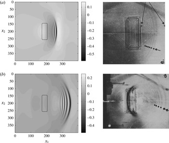
, are shown in figure 9. The leading wave trough is ahead of the topography by approximately half the length of the topography in figure 9(a). Six wave troughs are observed in the experiment, while the computation exhibits five troughs at
 ${\it\Omega}t={\rm\pi}$
, six troughs at
 ${\it\Omega}t=1.1{\rm\pi}$
and seven troughs at
 ${\it\Omega}t=1.2{\rm\pi}$
, see also figure 10(c,d). The leading wave trough is ahead of the topography by approximately the length of the topography at the later time
 ${\it\Omega}t=1.4{\rm\pi}$
(figure 9
b). The computation then exhibits 10 wave troughs with a trough-to-trough wavelength of
 $4.8h_{2}$
in the back part of the wave train, which is moving with the group velocity, see also figure 10(e). The number of waves indicated from the experiment is five (figure 9
b, right plot). (Note that the geometry is not moving for
 ${\it\Omega}t\geqslant {\rm\pi}$
.)
(a) Wave formation at (a)
 ${\it\Omega}t={\rm\pi}$
(half-cycle), computation (left), experiment by Maxworthy (Reference Maxworthy1979, figure 8e) (right), (b)
 ${\it\Omega}t=1.4{\rm\pi}$
, computation (left), experiment by Maxworthy (Reference Maxworthy1979, figure 9g) (right).
 $\mathit{Fr}=0.5$
,
 $d_{m}/H=0.5$
,
 ${\it\Omega}h_{2}/c_{0}=1/70$
.

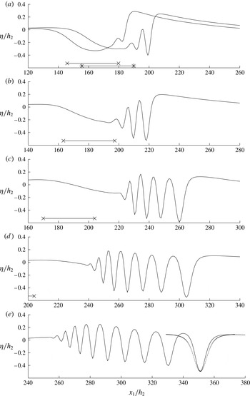
Elevation
 ${\it\eta}$
at mid-section versus
 $x_{1}$
for fixed
 $x_{2}=200h_{2}$
. (a)
 ${\it\Omega}t=0.6{\rm\pi}$
and
 $0.7{\rm\pi}$
, (b)
 ${\it\Omega}t=0.8{\rm\pi}$
, (c)
 ${\it\Omega}t={\rm\pi}$
, (d)
 ${\it\Omega}t=1.2{\rm\pi}$
, (e)
 ${\it\Omega}t=1.4{\rm\pi}$
. Positions of
 $x_{a}$
and
 $x_{b}$
of geometry indicated by
 $\times$
(
 ${\it\Omega}t=0.6{\rm\pi}$
,
 $0.8{\rm\pi}$
,
 ${\rm\pi}$
) and
 $\ast$
(
 $0.7{\rm\pi}$
).
 $\mathit{Fr}=0.5$
,
 $d_{m}/H=0.5$
. Dotted line in (e) shows a two-dimensional fully nonlinear solitary wave calculation with a reference level of
 $y_{0}=0.096h_{2}$
, depth ratio
 $(h_{1}+y_{0})/(h_{2}-y_{0})=17.36$
and amplitude
 $a/(h_{2}-y_{0})=0.6527$
.

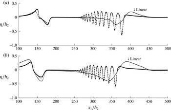
Figure 10 plots the calculated wave elevation along the mid-section of the tank (
 $x_{2}=200h_{2}$
) as function of
 $x_{1}$
at different times during the wave generation process,
 $0.6{\rm\pi}\leqslant {\it\Omega}t\leqslant 1.4{\rm\pi}$
. The location of the topography is indicated by the coordinates
 $x_{1}^{a}$
and
 $x_{1}^{b}$
, where
 $x_{1}^{b}-x_{1}^{a}=34h_{2}$
, see (5.1). The wave formation begins when the interface is sufficiently steep, at the leading face of the obstacle, for
 ${\it\Omega}t=0.6{\rm\pi}$
. Two troughs are formed at
 ${\it\Omega}t=0.7{\rm\pi}$
and three at
 ${\it\Omega}t=0.8{\rm\pi}$
. The number of waves behind the leading trough increases with time. So also does the trough-to-trough wavelength. The trough-to-crest height of the leading wave is
 $0.67h_{2}$
at
 ${\it\Omega}t={\rm\pi}$
and reduces to
 $0.59h_{2}$
at
 $1.4{\rm\pi}$
. The leading wave widens monotonically. However, the wave is far more narrow than a two-dimensional fully nonlinear solitary wave of corresponding amplitude (figure 10
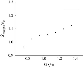
e). The speed of the leading depression is supercritical for
 ${\it\Omega}t>0.8{\rm\pi}$
, where the reference speed
 $\tilde{c}_{0}$
is calculated from the depth ratio at the positive elevation preceding the leading trough. At
 ${\it\Omega}t=1.4{\rm\pi}$
the excess speed of the leading depression,
 ${\dot{X}}_{trough}/\tilde{c}_{0}-1$
, is approximately half the perfect solitary wave excess speed, as illustrated in figure 11. The differences in the wave shape and propagation speed of the three-dimensional transient wave and the perfect solitary wave in two dimensions illustrate differences in the three- and two-dimensional wave generation processes. The lateral leakage of energy adds to the weakening of the leading trough in the three-dimensional case. The transient two-dimensional case is also slow in obtaining perfect solitary waves (Grue et al.
Reference Grue, Friis, Palm and Rusås1997, figure 9). The fully nonlinear solitary wave calculation has been performed using the method in Grue et al. (Reference Grue, Jensen, Rusås and Sveen1999) with a local reference level of
 $y_{0}=0.096h_{2}$
, local depth ratio
 $(h_{1}+y_{0})/(h_{2}-y_{0})=17.36$
and local amplitude
 $a/(h_{2}-y_{0})=0.6527$
. The soliton speed is 1.2399.


6. Simulations in relation to field measurements
Palmer et al. (Reference Palmer, Inall and Sharples2013) have measured strong internal waves generated along the seasonal thermocline at Jones Bank in the Celtic Sea. The spatio-temporal flow generated during the tidal cycle was in hydraulic control with supercritical velocity at the bank crest. A vertical depression of the thermocline, down to 40 m, corresponding to half the local water depth at the bank, was observed. In a complementary numerical study, Vlasenko et al. (Reference Vlasenko, Stashchuk, Palmer and Inall2013) used the MITgcm-code to simulate two different wave scenarios in the field experiments, obtaining three wave trains per tidal cycle in each of them. The wave trains were sketched in Vlasenko et al. (Reference Vlasenko, Stashchuk, Palmer and Inall2013, figures 6a, 11); no direct wave calculations were presented.
The observations by Palmer et al. (Reference Palmer, Inall and Sharples2013) and the simulations by Vlasenko et al. (Reference Vlasenko, Stashchuk, Palmer and Inall2013) have motivated the model calculations of the temporal three-dimensional flow features at the bank. We note that the present model does not take into account the rotational effects which are present in the oceanic setting. While the wave generation simulations during a short time frame may be realistic, the subsequent wave evolution is modified by rotational effects, see also the discussion in § 3.1.1 above.
The stratified sea has a thermocline with an average depth of approximately 40 m and is taken as the upper layer depth, i.e.
 $h_{2}=40~\text{m}$
. The value of
 $c_{0}\simeq 0.45~\text{m}~\text{s}^{-1}$
is obtained from the stratification (Vlasenko et al.
Reference Vlasenko, Stashchuk, Palmer and Inall2013, figure 3). The bank has a width at its half-height of approximately 4 km and length approximately three times the width. The non-dimensional width and length at the bank’s half-height become
 $w=100h_{2}$
and
 $l=300h_{2}$
, respectively. The model geometry of the bank is given by
 ${\it\delta}(x_{1},x_{2})=d_{m}\exp [-(|x_{1}-x_{10}|/(w/2))^{3}-(|x_{2}-x_{20}|/(l/2))^{3}]$
, where
 $d_{m}$
denotes the height of the bank. This is 50 m, and in the calculations is set to
 $1.2h_{2}$
. The horizontal location of the summit of the bank is determined by
 $(x_{10},x_{20})$
. In the present calculations we mimic the tidal flow by moving
 $(x_{10},x_{20})$
in an elliptical fashion. The depth outside the bank of 130 m gives
 $h_{1}/h_{2}=2.25$
.
The
 $M_{2}$
-tide has velocities of
 $(u_{1},u_{2})=(0.224,0.360)~\text{m}~\text{s}^{-1}$
along the (width, length)-directions of the bank, which in non-dimensional terms become
 $(u_{1},u_{2})/c_{0}\sim (0.5,0.8)$
(Palmer et al.
Reference Palmer, Inall and Sharples2013, figure 3 and table 1). Vlasenko et al. (Reference Vlasenko, Stashchuk, Palmer and Inall2013) have stressed the importance of an additional background current of
 $0.05~\text{m}~\text{s}^{-1}$
across the bank, corresponding to an increase in
 $u_{1}/c_{0}\simeq 0.1$
. The effect of the background current is accounted for by increasing
 $(u_{1},u_{2})/c_{0}$
from (0.5, 0.8) to (0.6, 0.8) in the calculations below, where the model geometry is moved according to
 $({\dot{x}}_{10},{\dot{x}}_{20})=(U_{M}\sin {\it\Omega}t,V_{M}\cos {\it\Omega}t)$
. Both topography and fluid are initially at rest. A smooth ramp-up of
 ${\dot{x}}_{20}$
is employed. The computational domain is
 $400h_{2}$
by
 $600h_{2}$
, with 720 nodes in each direction. The tidal frequency of
 ${\it\Omega}=2{\rm\pi}/12.4~\text{h}^{-1}$
becomes in non-dimensional terms
 ${\it\Omega}h_{2}/c_{0}\simeq 1/80$
.
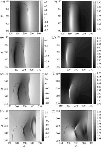
Simulations with
 $(u_{1},u_{2})/c_{0}=(0.6,0.8)$
show:
-
(i) For time
${\it\Omega}t=0.6{\rm\pi}$
,
$({\dot{x}}_{10},{\dot{x}}_{20})/c_{0}=(0.57,-0.25)$
, an elevation at
$x_{1}=240h_{2}$
extends for
$150h_{2}<x_{2}<350h_{2}$
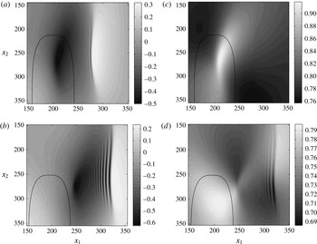
(figure 12
a). A depression and a large bottom velocity is formed above the bank for
$x_{1}=160h_{2}$
and
$150h_{2}<x_{2}<350h_{2}$
. The bottom velocity, obtained in the frame of reference fixed to the bank, i.e.
$\boldsymbol{v}_{b}=\boldsymbol{{\rm\nabla}}{\it\phi}_{1}-({\dot{x}}_{10},{\dot{x}}_{20})$
at
$B$
, is subcritical and up to
$0.9c_{0}$
(figure 12
e). -
(ii) For
${\it\Omega}t=0.8{\rm\pi}$
,
$({\dot{x}}_{10},{\dot{x}}_{20})/c_{0}=(0.35,-0.65)$
, the elevation at
$x_{1}=250h_{2}{-}260h_{2}$
and depression at
$x_{1}=180{-}190h_{2}$
and
$210h_{2}<x_{2}<320h_{2}$
have slightly positive curvature in the
$x_{1}$
-direction (figure 12
b). The bottom velocity is supercritical with a magnitude of up to
$1.15c_{0}$
for
$x_{1}=180h_{2}{-}190h_{2}$
and
$230h_{2}<x_{2}<320h_{2}$
(figure 12
f). The region of supercritical velocity above the bank has a slight positive curvature in the
$x_{1}$
-direction. -
(iii) For
${\it\Omega}t=0.95{\rm\pi}$
,
$({\dot{x}}_{10},{\dot{x}}_{20})/c_{0}=(0.09,-0.79)$
, a wave train appears behind the elevation at
$x_{1}=270h_{2}{-}280h_{2}$
. The curved depression over the bank at
$x_{1}=200{-}220h_{2}$
and
$230h_{2}<x_{2}<320h_{2}$
is more pronounced (figure 12
c). The three-dimensional region of supercritical bottom velocity (up to
$1.2c_{0}$
) is similarly curved (figure 12
g). -
(iv) For time
${\it\Omega}t=1.15{\rm\pi}$
,
$({\dot{x}}_{10},{\dot{x}}_{20})/c_{0}=(-0.27,-0.71)$
, the wave train behind the elevation at
$x_{1}=320h_{2}$
has height up to
$1.2h_{2}$
. The crests are straight. A second wave train develops behind the interfacial trough previously located above the bank, now at
$x_{1}\sim 240h_{2}$
. This wave train curves along the
$x_{1}$
-direction (figure 12
d,h).








(a–d) Interfacial elevation
 ${\it\eta}/h_{2}$
and (e–h) bottom velocity
 $|\boldsymbol{v}_{b}|/c_{0}$
, where
 $\boldsymbol{v}_{b}$
is the fluid velocity at the sea bottom, obtained in the frame of reference following the bank, for (a,e)
 ${\it\Omega}t=0.6{\rm\pi}$
, (b,f)
 ${\it\Omega}t=0.8{\rm\pi}$
, (c,g)
 ${\it\Omega}t=0.95{\rm\pi}$
, (d,h)
 ${\it\Omega}t=1.15{\rm\pi}$
. Current ellipse
 $(u_{1},u_{2})/c_{0}=(0.6,0.8)$
.
 $h_{1}/h_{2}=2.25$
,
 $d_{m}/h_{2}=1.2$
,
 ${\it\Omega}h_{2}/c_{0}=1/86$
. Position of topography indicated by the contour line at half-height. Velocity of topography
 $({\dot{x}}_{10},{\dot{x}}_{20})/c_{0}$
given in the main text.

Simulations with the weaker excitation of
 $(u_{1},u_{2})/c_{0}=(0.5,0.8)$
show that for
 ${\it\Omega}t=0.95{\rm\pi}$
,
 $({\dot{x}}_{10},{\dot{x}}_{20})/c_{0}=(0.08,-0.79)$
, a weak wave train develops behind the elevation at
 $x_{1}=270h_{2}{-}280h_{2}$
. The much weaker depression over the bank at
 $x_{1}=210h_{2}$
,
 $x_{2}=250h_{2}$
causes a subcritical bottom velocity (figure 13
a,c). For time
 ${\it\Omega}t=1.15{\rm\pi}$
only one wave train behind the elevation, at
 $x_{1}=320h_{2}$
with height up to
 $0.8h_{2}$
, is formed (figure 13
b,d).
Same as figure 12 for
 ${\it\Omega}t=0.95{\rm\pi}$
(a,c);
 ${\it\Omega}t=1.15{\rm\pi}$
(b,d); current ellipse
 $(u_{1},u_{2})/c_{0}=(0.5,0.8)$
.

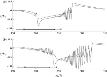
Sections of
 ${\it\eta}/h_{2}$
, for fixed
 $x_{2}/h_{2}=280$
, illustrate the two wave trains for the strong and weak excitations, obtained for
 ${\it\Omega}t=0.95{\rm\pi}$
and
 ${\it\Omega}t=1.15{\rm\pi}$
. The wavelength is in the range
 ${\it\lambda}\sim 7h_{2}{-}3h_{2}$
(figure 14). The upstream wave train is much stronger than the downstream wave train, in the strong excitation. Only the upstream wave train is visible for the weak excitation. The leading depression of the dominant wave train in figure 14(a,b) moves a distance of approximately
 $40h_{2}$
between
 ${\it\Omega}t=0.95{\rm\pi}$
and
 ${\it\Omega}t=1.15{\rm\pi}$
. The change in position is only slightly influenced by the topography. The other depression moves a distance of approximately
 $35h_{2}$
between
 ${\it\Omega}t=0.95{\rm\pi}$
and
 ${\it\Omega}t=1.15{\rm\pi}$
. The local depth of the topography somewhat influences the wave propagation.
Interfacial elevation
 ${\it\eta}/h_{2}$
. Section along
 $x_{2}=280h_{2}$
, for strong
 $(u_{1},u_{2})/c_{0}=(0.6,0.8)$
and weak
 $(u_{1},u_{2})/c_{0}=(0.5,0.8)$
excitation. (a)
 ${\it\Omega}t=0.95{\rm\pi}$
; (b)
 ${\it\Omega}t=1.15{\rm\pi}$
.
 $h_{1}/h_{2}=2.25$
,
 $d_{m}/h_{2}=1.2$
. Horizontal position of the geometry at its half-height indicated by
 $\ast$
—
 $\ast ~(u_{1},u_{2})/c_{0}=(0.6,0.8)$
,
 $\times$
—
 $\times$
 $(u_{1},u_{2})/c_{0}=(0.5,0.8)$
.

These model simulations show, for a time period somewhat longer than a half tidal cycle, i.e.
 $0<{\it\Omega}t<1.15{\rm\pi}$
, that two wave trains are generated for a tidal ellipse of strength
 $(u_{1},u_{2})/c_{0}=(0.6,0.8)$
, and one wave train for
 $(u_{1},u_{2})/c_{0}=(0.5,0.8)$
. The difference in
 $u_{1}/c_{0}$
between the two different scenarios corresponds to the small increase due to a background current of
 $0.05~\text{m}~\text{s}^{-1}$
in the observations by Palmer et al. (Reference Palmer, Inall and Sharples2013) and simulations by Vlasenko et al. (Reference Vlasenko, Stashchuk, Palmer and Inall2013). Thus, with a unidirectional background current across the bank, two wave trains are generated during the phase of strong excitation and one wave train during the phase of weak excitation – a total of three wave trains per tidal cycle.
7. Conclusion
We develop a two-layer mathematical interfacial wave model in three dimensions. The method is fully dispersive and strongly nonlinear and is here developed with complementary numerical implementation and testing. A set of integral equations couples the velocity potentials (tangential velocities) to the normal velocities along the lower and upper side of the interface. The interaction between the interfacial motion and a time-varying bottom topography is taken into account, where the bottom variation contributes to an additional coupled integral equation as well as integrals over the bottom variables.
The integral equations are at the onset fully nonlinear in the vertical excursions of the interface and bottom topography. The source and dipole terms appearing in the integral equations are developed in series expansions containing linear, quadratic, cubic and higher order terms. By means of successive approximations and application of the Fourier transform, explicit inversion of the integral equations is obtained in terms of series expansions. We find, for the applications in the present paper, calculating the formation of interfacial wave trains of non-dimensional amplitude up to unity, that the quadratic approximation contains the essential dynamics, while the additional cubic terms are very small. The quadratic and cubic approximations have been successfully compared to exact calculations of solitary waves over a flat bottom.
The three-dimensional method is used to calculate the curved wave train formation measured and visualized in experiments carried out by Maxworthy (Reference Maxworthy1979), where a topography was moved in an oscillatory manner mimicking a tidal oscillation. The computations confirm the transition observed in the experiments: wave trains are formed when the Froude number (
 $\mathit{Fr}$
) obtained from the maximum speed of the topography divided by the linear internal long-wave speed exceeds a certain value, depending on the height of the geometry relative to the fluid layer depth. The leading depression wave is found to be narrower than a fully developed two-dimensional solitary wave of comparable amplitude, while the excess speed is approximately half that of the solitary wave.
We also perform a set of calculations relevant to tidally driven highly nonlinear and three-dimensional internal wave formation at the Jones Bank in the Celtic Sea. The calculations are motivated by recent field observations (Palmer et al.
Reference Palmer, Inall and Sharples2013) and numerical ocean modelling calculations (Vlasenko et al.
Reference Vlasenko, Stashchuk, Palmer and Inall2013, Reference Vlasenko, Stashchuk, Inall and Hopkins2014). Using the linear long-wave speed
 $c_{0}$
as the velocity scale, the tidal ellipse observed in the field becomes in non-dimensional terms
 $(u_{1},u_{2})/c_{0}=(0.5,0.8)$
. The velocity components are across/along the bank. Simulations during a half tidal cycle, with two different tidal ellipses, of (0.6, 0.8) and (0.5, 0.8), show that two wave trains are formed in the former case and one wave train in the latter. One of the wave trains has forward curvature and is dictated by the curved strong depression over the bank. Rotational effects are not accounted for in the present model, see comments in § 3.1.1.
Appendix A. Expansions of the Green functions
The contributions from the Green function in (2.3) are expanded in power series of
 ${\it\eta}$
and
 ${\it\delta}$
as
 $$\begin{eqnarray}\displaystyle \frac{1}{r}+\frac{1}{r_{1}} & = & \displaystyle \frac{1}{R}+\frac{1}{R_{1}}+({\it\eta}+{\it\eta}^{\prime })\frac{\partial }{\partial (2h_{1})}\frac{1}{R_{1}}-\frac{1}{2}({\it\eta}-{\it\eta}^{\prime })^{2}\boldsymbol{{\rm\nabla}}_{H}^{^{\prime }2}\frac{1}{R}\nonumber\\ \displaystyle & & \displaystyle +\,\frac{1}{2}({\it\eta}+{\it\eta}^{\prime })^{2}\frac{\partial ^{2}}{\partial (2h_{1})^{2}}\frac{1}{R_{1}}+\cdots \,,\nonumber\\ \displaystyle & & \displaystyle \quad (\boldsymbol{x},y)\text{ on }I,(\boldsymbol{x}^{\prime },y^{\prime })\text{ on }I,\end{eqnarray}$$
 $$\begin{eqnarray}\displaystyle \frac{1}{r}+\frac{1}{r_{1}} & = & \displaystyle \frac{2}{R_{0}}+2{\it\eta}\frac{\partial }{\partial h_{1}}\frac{1}{R_{0}}+({\it\eta}^{2}+{\it\delta}^{\prime 2})\frac{\partial ^{2}}{\partial h_{1}^{2}}\frac{1}{R_{0}}+\cdots \,,\quad \nonumber\\ \displaystyle & & \displaystyle \quad (\boldsymbol{x},y)\text{ on }I,(\boldsymbol{x}^{\prime },y^{\prime })\text{ on }B,\end{eqnarray}$$
 $$\begin{eqnarray}\displaystyle \left(\frac{\partial }{\partial y^{\prime }}-\boldsymbol{{\rm\nabla}}_{H}^{\prime }{\it\eta}^{\prime }\boldsymbol{\cdot }\boldsymbol{{\rm\nabla}}_{H}^{\prime }\right)\left(\frac{1}{r}+\frac{1}{r_{1}}\right) & = & \displaystyle \frac{\partial }{\partial (2h_{1})}\frac{1}{R_{1}}-\boldsymbol{{\rm\nabla}}_{H}^{\prime }\boldsymbol{\cdot }\left(({\it\eta}^{\prime }-{\it\eta})\boldsymbol{{\rm\nabla}}_{H}^{\prime }\frac{1}{R}\right)\nonumber\\ \displaystyle & & \displaystyle -\,\boldsymbol{{\rm\nabla}}_{H}^{\prime }\boldsymbol{\cdot }\left(({\it\eta}^{\prime }+{\it\eta})\boldsymbol{{\rm\nabla}}_{H}^{\prime }\frac{1}{R_{1}}\right)\nonumber\\ \displaystyle & & \displaystyle -\,\boldsymbol{{\rm\nabla}}_{H}^{\prime }\boldsymbol{\cdot }\left(\frac{1}{2}({\it\eta}^{\prime }+{\it\eta})^{2}\boldsymbol{{\rm\nabla}}_{H}^{\prime }\frac{\partial }{\partial (2h_{1})}\frac{1}{R_{1}}\right)+\cdots \,,\quad \nonumber\\ \displaystyle & & \displaystyle \quad (\boldsymbol{x},y)\text{ on }I,(\boldsymbol{x}^{\prime },y^{\prime })\text{ on }I,\end{eqnarray}$$
 $$\begin{eqnarray}\displaystyle \left(-\frac{\partial }{\partial y^{\prime }}+\boldsymbol{{\rm\nabla}}_{H}^{\prime }{\it\delta}^{\prime }\boldsymbol{\cdot }\boldsymbol{{\rm\nabla}}_{H}^{\prime }\right)\left(\frac{1}{r}+\frac{1}{r_{1}}\right) & = & \displaystyle 2\boldsymbol{{\rm\nabla}}_{H}^{\prime }\boldsymbol{\cdot }\left({\it\delta}^{\prime }\boldsymbol{{\rm\nabla}}_{H}^{\prime }\frac{1}{R_{0}}\right)\nonumber\\ \displaystyle & & \displaystyle +\,2{\it\eta}\boldsymbol{{\rm\nabla}}_{H}^{\prime }\boldsymbol{\cdot }\left({\it\delta}^{\prime }\boldsymbol{{\rm\nabla}}_{H}^{\prime }\frac{\partial }{\partial h_{1}}\frac{1}{R_{0}}\right)+\cdots \,,\nonumber\\ \displaystyle & & \displaystyle \quad (\boldsymbol{x},y)\text{ on }I,(\boldsymbol{x}^{\prime },y^{\prime })\text{ on }B.\end{eqnarray}$$
In (A 1)–(A 4),
 $R_{1}=\sqrt{R^{2}+4h_{1}^{2}}$
and
 $R_{0}=\sqrt{R^{2}+h_{1}^{2}}$
.
 $\boldsymbol{{\rm\nabla}}_{H}$
denotes horizontal gradient.
The contributions from the Green function in (2.4) are expanded similarly in
 ${\it\eta}$
and
 ${\it\delta}$
as
 $$\begin{eqnarray}\displaystyle \frac{1}{r}+\frac{1}{r_{1B}} & = & \displaystyle \frac{1}{R}+\frac{1}{R_{1}}-({\it\delta}^{\prime }+{\it\delta})\frac{\partial }{\partial (2h_{1})}\frac{1}{R_{1}}\nonumber\\ \displaystyle & & \displaystyle -\,\frac{1}{2}({\it\delta}^{\prime }-{\it\delta})^{2}\boldsymbol{{\rm\nabla}}_{H}^{^{\prime }2}\frac{1}{R}+\frac{1}{2}({\it\delta}^{\prime }+{\it\delta})^{2}\frac{\partial ^{2}}{\partial (2h_{1})^{2}}\frac{1}{R_{1}}+\cdots \,,\quad \nonumber\\ \displaystyle & & \displaystyle \quad (\boldsymbol{x},y)\text{ on }B,(\boldsymbol{x}^{\prime },y^{\prime })\text{ on }B,\end{eqnarray}$$
 $$\begin{eqnarray}\displaystyle \frac{1}{r}+\frac{1}{r_{1B}} & = & \displaystyle \frac{2}{R_{0}}-2{\it\delta}\frac{\partial }{\partial h_{1}}\frac{1}{R_{0}}+({\it\delta}^{2}+{\it\eta}^{^{\prime }2})\frac{\partial ^{2}}{\partial h_{1}^{2}}\frac{1}{R_{0}}+\cdots \,,\quad \nonumber\\ \displaystyle & & \displaystyle \quad (\boldsymbol{x},y)\text{ on }B,(\boldsymbol{x}^{\prime },y^{\prime })\text{ on }I,\end{eqnarray}$$
 $$\begin{eqnarray}\displaystyle \left(-\frac{\partial }{\partial y^{\prime }}+\boldsymbol{{\rm\nabla}}_{H}^{\prime }{\it\delta}^{\prime }\boldsymbol{\cdot }\boldsymbol{{\rm\nabla}}_{H}^{\prime }\right)\left(\frac{1}{r}+\frac{1}{r_{1B}}\right) & = & \displaystyle \frac{\partial }{\partial (2h_{1})}\frac{1}{R_{1}}+\boldsymbol{{\rm\nabla}}_{H}^{\prime }\boldsymbol{\cdot }\left(({\it\delta}^{\prime }-{\it\delta})\boldsymbol{{\rm\nabla}}_{H}^{\prime }\frac{1}{R}\right)\nonumber\\ \displaystyle & & \displaystyle +\,\boldsymbol{{\rm\nabla}}_{H}^{\prime }\boldsymbol{\cdot }\left(({\it\delta}^{\prime }+{\it\delta})\boldsymbol{{\rm\nabla}}_{H}^{\prime }\frac{1}{R_{1}}\right)\nonumber\\ \displaystyle & & \displaystyle -\,\boldsymbol{{\rm\nabla}}_{H}^{\prime }\boldsymbol{\cdot }\left(\frac{1}{2}({\it\delta}^{\prime }+{\it\delta})^{2}\boldsymbol{{\rm\nabla}}_{H}^{\prime }\frac{\partial }{\partial (2h_{1})}\frac{1}{R_{1}}\right)+\cdots \quad \nonumber\\ \displaystyle & & \displaystyle \quad (\boldsymbol{x},y)\text{ on }B,(\boldsymbol{x}^{\prime },y^{\prime })\text{ on }B,\end{eqnarray}$$
 $$\begin{eqnarray}\displaystyle \left(\frac{\partial }{\partial y^{\prime }}-\boldsymbol{{\rm\nabla}}_{H}^{\prime }{\it\eta}^{\prime }\boldsymbol{\cdot }\boldsymbol{{\rm\nabla}}_{H}^{\prime }\right)\left(\frac{1}{r}+\frac{1}{r_{1B}}\right) & = & \displaystyle -2\boldsymbol{{\rm\nabla}}_{H}^{\prime }\boldsymbol{\cdot }\left({\it\eta}^{\prime }\boldsymbol{{\rm\nabla}}_{H}^{\prime }\frac{1}{R_{0}}\right)\nonumber\\ \displaystyle & & \displaystyle -\,2{\it\delta}\boldsymbol{{\rm\nabla}}_{H}^{\prime }\boldsymbol{\cdot }\left({\it\eta}^{\prime }\boldsymbol{{\rm\nabla}}_{H}^{\prime }\frac{\partial }{\partial h_{1}}\frac{1}{R_{0}}\right)+\cdots \nonumber\\ \displaystyle & & \displaystyle \quad (\boldsymbol{x},y)\text{ on }B,(\boldsymbol{x}^{\prime },y^{\prime })\text{ on }I.\end{eqnarray}$$
Appendix B. Expressions for
$V_{I}^{(3)}$
and
$W_{I}^{(3)}$


The normal velocity
 $V_{I}$
defined in (2.5) is obtained by the method of successive approximations, where
 $V_{I}=V_{I}^{(1)}+V_{I}^{(2)}+V_{I}^{(3)}+\cdots \,$
, see § 2.2.3.
 $V_{I}^{(1)}$
and
 $V_{I}^{(2)}$
are obtained in (2.10) and (2.11) and
 $V_{I}^{(3)}$
as
 $$\begin{eqnarray}\displaystyle \hat{V_{I}}^{(3)} & = & \displaystyle \frac{k}{1+e_{1}}(\hat{V_{I}}^{(3,1)}+\hat{V_{I}}^{(3,2)}+\hat{V_{I}}^{(3,3)}+\hat{V_{I}}^{(3,4)}),\end{eqnarray}$$
 $$\begin{eqnarray}\displaystyle \hat{V_{I}}^{(3,1)} & = & \displaystyle e_{1}\mathscr{F}[{\it\eta}(V_{I}-V_{I}^{(1)})]+\mathscr{F}\{{\it\eta}\mathscr{F}^{-1}[e_{1}(\hat{V_{I}}-\hat{V}_{I}^{(1)})]\},\end{eqnarray}$$
 $$\begin{eqnarray}\displaystyle \hat{V_{I}}^{(3,2)} & = & \displaystyle -{\textstyle \frac{1}{2}}k(1+e_{1})\mathscr{F}({\it\eta}^{2}V_{I})+\mathscr{F}\{{\it\eta}\mathscr{F}^{-1}[k(1-e_{1})\mathscr{F}({\it\eta}V_{I})]\}\nonumber\\ \displaystyle & & \displaystyle -\,{\textstyle \frac{1}{2}}\mathscr{F}\{{\it\eta}^{2}\mathscr{F}^{-1}[k(1+e_{1})\hat{V_{I}}]\},\end{eqnarray}$$
 $$\begin{eqnarray}\displaystyle \hat{V_{I}}^{(3,3)} & = & \displaystyle {\textstyle \frac{1}{2}}e_{1}\text{i}\boldsymbol{k}\boldsymbol{\cdot }\mathscr{F}({\it\eta}^{2}\boldsymbol{{\rm\nabla}}_{H}{\it\phi}_{1I})+\mathscr{F}\{{\it\eta}\mathscr{F}^{-1}[e_{1}\text{i}\boldsymbol{k}\boldsymbol{\cdot }\mathscr{F}({\it\eta}\boldsymbol{{\rm\nabla}}_{H}{\it\phi}_{1I})]\}\nonumber\\ \displaystyle & & \displaystyle -\,{\textstyle \frac{1}{2}}\mathscr{F}[{\it\eta}^{2}\mathscr{F}^{-1}(e_{1}k^{2}\hat{{\it\phi}}_{1I})],\end{eqnarray}$$
 $$\begin{eqnarray}\displaystyle \hat{V}^{(3,4)} & = & \displaystyle -\mathscr{F}({\it\eta}^{2}\mathscr{F}^{-1}[k\sqrt{e_{1}}\hat{V}_{B}])-k\sqrt{e_{1}}\mathscr{F}({\it\delta}^{2}V_{B})\nonumber\\ \displaystyle & & \displaystyle -\,\mathscr{F}({\it\eta}\mathscr{F}^{-1}[2\sqrt{e_{1}}\text{i}\boldsymbol{k}\boldsymbol{\cdot }\mathscr{F}({\it\delta}\boldsymbol{{\rm\nabla}}_{H}{\it\phi}_{1B})]),\end{eqnarray}$$
 $e_{1}=\text{e}^{-2kh_{1}}$
.
The normal velocity
 $W_{I}=W_{I}^{(1)}+W_{I}^{(2)}+W_{I}^{(3)}+\cdots \!\;$
defined in § 2.2.4 is obtained similarly, with
 $W_{I}^{(1)}$
and
 $W_{I}^{(2)}$
obtained in (2.14) and (2.15) and
 $W_{I}^{(3)}$
as
 $$\begin{eqnarray}\displaystyle {\hat{W}}_{I}^{(3)} & = & \displaystyle \frac{k}{1+e_{2}}\left({\hat{W}}_{I}^{(3,1)}+{\hat{W}}_{I}^{(3,2)}+{\hat{W}}_{I}^{(3,3)}\right),\end{eqnarray}$$
 $$\begin{eqnarray}\displaystyle {\hat{W}}_{I}^{(3,1)} & = & \displaystyle -e_{2}\mathscr{F}[{\it\eta}(W_{I}-W_{I}^{(1)})]-\mathscr{F}\{{\it\eta}\mathscr{F}^{-1}[e_{2}({\hat{W}}_{I}-{\hat{W}}_{I}^{(1)})]\},\end{eqnarray}$$
 $$\begin{eqnarray}\displaystyle {\hat{W}}_{I}^{(3,2)} & = & \displaystyle -{\textstyle \frac{1}{2}}k(1+e_{2})\mathscr{F}({\it\eta}^{2}W_{I})+\mathscr{F}\{{\it\eta}\mathscr{F}^{-1}[k(1-e_{2})\mathscr{F}({\it\eta}W_{I})]\}\nonumber\\ \displaystyle & & \displaystyle -\,{\textstyle \frac{1}{2}}\mathscr{F}\{{\it\eta}^{2}\mathscr{F}^{-1}[k(1+e_{2})\hat{W_{I}}]\},\end{eqnarray}$$
 $$\begin{eqnarray}\displaystyle {\textstyle \frac{1}{2}}W_{I}^{(3,3)} & = & \displaystyle -{\textstyle \frac{1}{2}}e_{2}\text{i}\boldsymbol{k}\boldsymbol{\cdot }\mathscr{F}({\it\eta}^{2}\boldsymbol{{\rm\nabla}}_{H}{\it\phi}_{2I})-\mathscr{F}\{{\it\eta}\mathscr{F}^{-1}[e_{2}\text{i}\boldsymbol{k}\boldsymbol{\cdot }\mathscr{F}({\it\eta}\boldsymbol{{\rm\nabla}}_{H}{\it\phi}_{2I})]\}\nonumber\\ \displaystyle & & \displaystyle +\,{\textstyle \frac{1}{2}}\mathscr{F}[{\it\eta}^{2}\mathscr{F}^{-1}(e_{2}k^{2}{\it\phi}_{2I})],\end{eqnarray}$$
 $e_{2}=\text{e}^{-2kh_{2}}$
.