1 Introduction
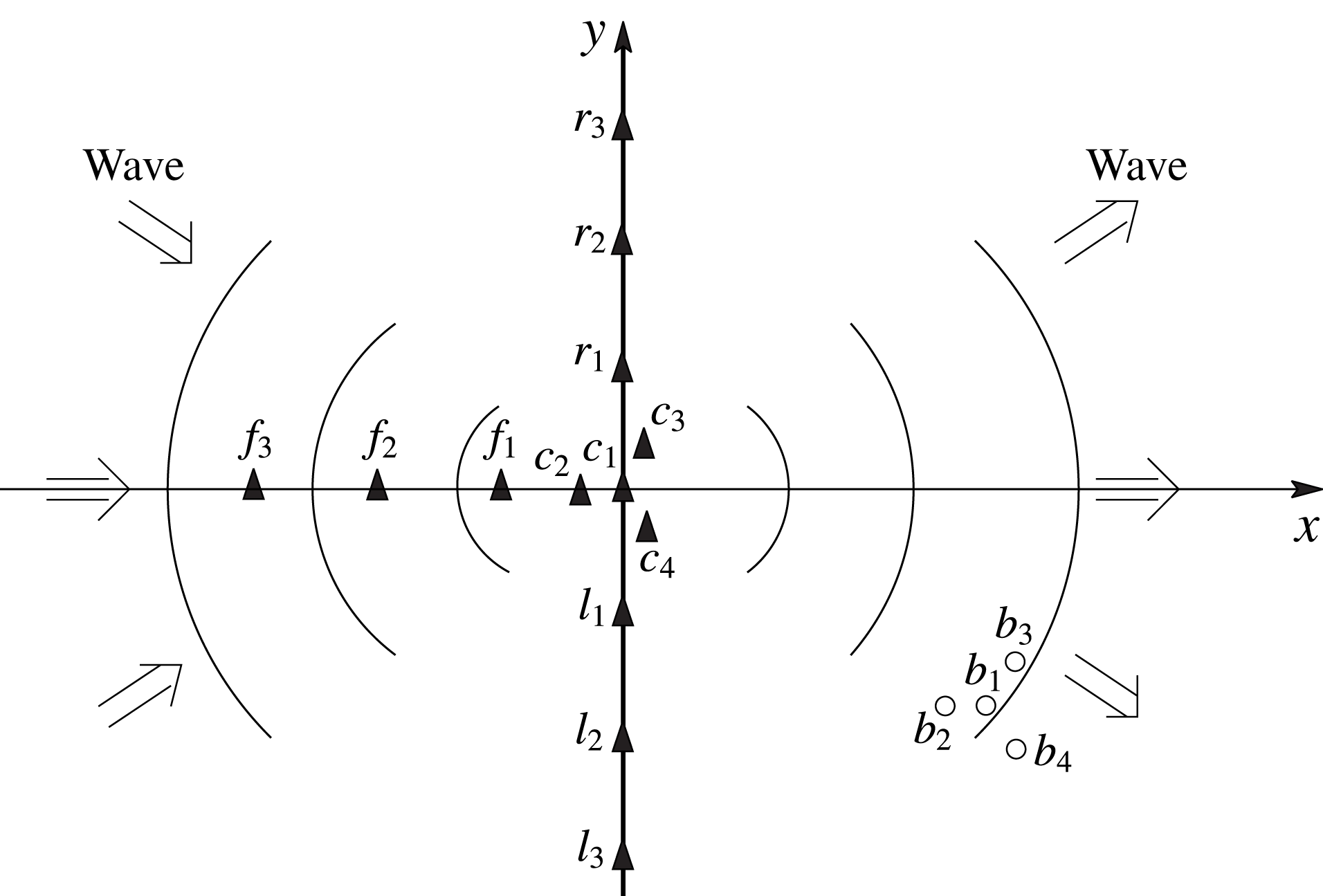
An important open problem in ocean engineering both in the field and in wave basins, is the ability to reconstruct the phase-resolved wave field that matches a given set of spatial/temporal measurements, in some space–time domain
 ${\mathcal{M}}$
, of an underlying, generally nonlinear, wave field. For an underlying wave field represented by, say, velocity potential
 $\tilde{\unicode[STIX]{x1D6F7}}(\boldsymbol{x},z,t)$
, the objective is to obtain the phase-resolved ‘reconstructed’ wave field
 $\unicode[STIX]{x1D6F7}(\boldsymbol{x},z,t)$
that predicts
 $\tilde{\unicode[STIX]{x1D6F7}}$
in some ‘predictable zone’
 ${\mathcal{P}}$
in space–time. Generally
 ${\mathcal{P}}$
is greater than
 ${\mathcal{M}}$
(
 ${\mathcal{P}}\supset {\mathcal{M}}$
), so that one is able to forecast into later times or larger domains beyond the measurements in
 ${\mathcal{M}}$
.
In a related work, Qi et al. (Reference Qi, Wu, Liu and Yue2018) developed a theoretical approach, valid for different measurements
 ${\mathcal{M}}$
, to obtain the linear predictable zone, hereafter referred to as
 ${\mathcal{P}}_{L}$
, in the context of linearized wave theory. However, they do not address how the reconstructed wave field can actually be obtained in the predictable zone. The main focus of this work is to develop and test an approach for the reconstruction of a general nonlinear wave field.
Assuming linearized theory, any set of measurements in a given
 ${\mathcal{M}}$
can in theory be matched by sufficiently large number of (independent) free wave modes. For example, if the wave elevation
 $\unicode[STIX]{x1D701}(t)$
of a unidirectional wave field is measured at some location
 $\boldsymbol{x}=\unicode[STIX]{x1D743}$
over a period of time
 $T$
, a Fourier series with sufficient terms could match
 $\unicode[STIX]{x1D701}(t\in T)$
to any precision in
 ${\mathcal{M}}$
, regardless of whether
 $\unicode[STIX]{x1D701}$
measures a linear or nonlinear wave. However, for waves with even relatively small steepnesses commonly encountered in practice, the wave field described by these components would not in general describe accurately other quantities such as velocity or pressure under this surface, nor even the surface elevation (far) outside of the measurement
 ${\mathcal{M}}$
. We illustrate this later by comparing linear versus nonlinear reconstructed wave fields against synthetic waves (cf. § 3.1.1) and tank measurements (cf. § 3.1.3).
A general nonlinear wave field contains free propagating wave components as well as ‘locked’ components due to nonlinear wave–wave interactions. A nonlinear reconstruction must account for all these components in matching the measurements. There are relatively small number of studies that include nonlinearity in reconstruction, for example, Stansberg (Reference Stansberg1993) and Zhang et al. (Reference Zhang, Chen, Ye and Randall1996, Reference Zhang, Yang, Wen, Prislin and Hong1999), which include up to second-order wave nonlinearity. Since the wave field can be represented in closed form up to second order, the reconstruction is still relatively simple. However, it is not straightforward to extend such approaches to higher order. In this study (§§ 3 and 2.5), we show that inclusion of the higher-order nonlinear effects is very important in the reconstruction of steeper wave fields. Recently, Simanesew et al. (Reference Simanesew, Trulsen, Krogstad and Nieto-Borge2017) considered reconstruction/prediction of sufficiently narrow-banded waves using a third-order modified nonlinear Schrödinger equation (MNLS) as the model equation. For long-crested narrow-banded waves, they obtain correct predictions over certain distances, which they show is strongly reduced for short-crested waves with increasing directional spread. The range of applicability of MNLS reconstruction for general broad-banded wave fields is difficult to assess due to the assumptions inherent in the MNLS. Significantly, none of the existing work provides the predictable zone
 ${\mathcal{P}}$
, for a given set of measurements
 ${\mathcal{M}}$
, within which the linear or nonlinear reconstructed wave-field prediction can be assumed correct without actual knowledge of the underlying wave field.
In this work, we address the problem of nonlinear phase-resolved reconstruction of general two- and three-dimensional wave fields. We assume that the measurements are of sufficient duration and resolution to resolve the frequencies and directions of the wave components in
 ${\mathcal{M}}$
. To make the problem well defined (and solvable), we assume that wave components that pass through
 ${\mathcal{M}}$
, and are measured, propagate unchanged from
 ${\mathcal{M}}$
, i.e. there are no (unknown) disturbances, forcing or dissipation of these measured wave components between
 ${\mathcal{M}}$
and the predicted zone
 ${\mathcal{P}}$
. The problem is non-trivial in that we do not assume the same anywhere else in the wave field, outside of
 ${\mathcal{M}}$
and the domain where the measured components propagate.
For a given set of measurements
 ${\mathcal{M}}$
, the reconstruction problem is a nonlinear inverse problem, in which we aim to reconstruct a (theoretically) continuous nonlinear system using a representation with a finite number of model parameters. Due to data insufficiency, it is strictly impossible to uniquely determine all the details of the original system. For linear inverse problems, however, it has been shown that certain properties, such as local estimation, of the original system can be obtained from the reconstructed model (Backus & Gilbert Reference Backus and Gilbert1968). For nonlinear inverse problems (Snieder Reference Snieder1998), the model reconstruction becomes much more difficult. For strongly nonlinear problems, there is no systematic way to reconstruct the model and the inverse Monte Carlo sampling method (Mosegaard Reference Mosegaard1998) is probably the only available way to estimate the model.
In this work, we restrict our attention to nonlinear waves which can be uniquely expressed as regular perturbation series of arbitrary high order in wave steepness. Under this restriction, it has been shown (Snieder Reference Snieder1991) that a high-order model can be reconstructed to obtain an optimal and unique local estimation of the original nonlinear system. Our objective is to develop this high-order phase-resolved reconstruction and to assess its feasibility, validity and efficacy by applying it to a broad ranges of wave-field conditions and measurements, including nonlinear wave fields generated numerically and in physical wave experiments. Specifically, we develop an iterative high-order reconstruction (HOR) method which accounts for nonlinear wave interactions up to some order
 $M$
in wave steepness. HOR optimizes the amplitude and phase of a number (
 $L$
) of free wave components, based on which all high-order locked wave components can be determined by solving the Euler equations. By iteratively increasing
 $M$
and
 $L$
, HOR obtains a wave field that minimizes the reconstruction error between the reconstructed field and given measurements. HOR provides the phase-resolved whole field description of the nonlinear waves including wave elevation, velocity and pressure, which we use to compare and evaluate against the larger underlying wave field from which the measurements are taken (beyond
 ${\mathcal{M}}$
).
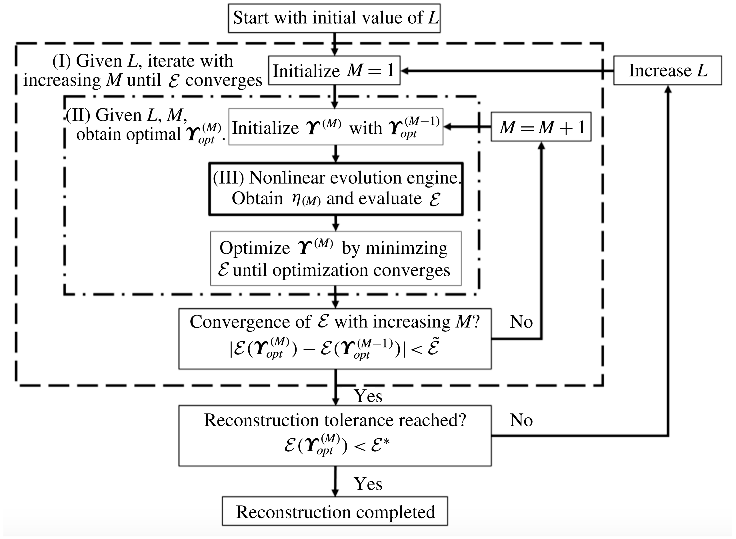
HOR requires a computationally efficient general phase-resolved ‘nonlinear evolution engine’ which is ‘evaluated’ repeatedly in minimizing the reconstruction error in
 ${\mathcal{M}}$
(cf. figure 1). To achieve this, we implement the high-order spectral (HOS) method (Dommermuth & Yue Reference Dommermuth and Yue1987) in HOR. Given an initial field defined by the HOR model parameters, HOS solves the Euler equations using
 $N$
spectral modes up to a specified nonlinear order
 $M$
in wave steepness. HOS obtains exponential convergence with
 $N$
and
 $M$
, and has operation count that scales linearly with
 $N$
and
 $M$
. In terms of the requirements of the present HOR scheme, HOS is, in many ways, an ideal evolution engine.
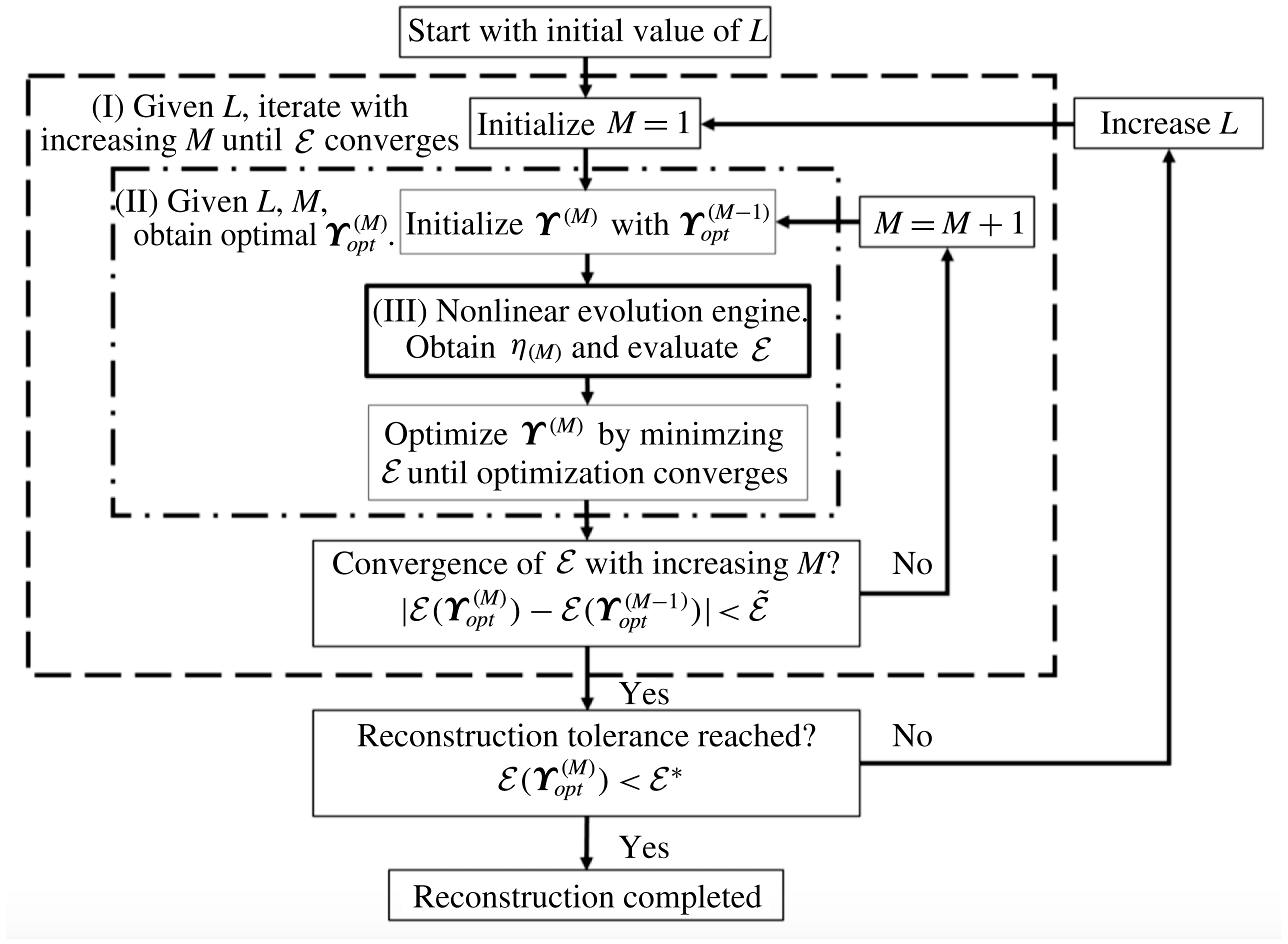
The flow chart for the nonlinear reconstruction scheme using HOR.
We evaluate the validity and performance of HOR. We also address a number of theoretical and practical issues associated with HOR which include: (i) convergence of the HOR scheme to a unique solution
 $\unicode[STIX]{x1D6F7}$
close to the underlying wave field
 $\tilde{\unicode[STIX]{x1D6F7}}$
in some nonlinear predictable zone
 ${\mathcal{P}}_{NL}$
beyond the measurements
 ${\mathcal{M}}$
; (ii) the space–time extent of
 ${\mathcal{P}}_{NL}$
and its relationship to the linear predictable zone
 ${\mathcal{P}}_{L}$
which can be theoretically obtained given
 ${\mathcal{M}}$
(Qi et al.
Reference Qi, Wu, Liu and Yue2018); (iii) importance of high-order nonlinear effects in the reconstruction in predicting
 $\tilde{\unicode[STIX]{x1D6F7}}$
; and (iv) the computational efficacy of HOR, related to the number of HOS ‘evaluations’
 $N_{eval}$
, which depends on the number of HOR wave-field model parameters
 $L$
, and the nonlinear order
 $M$
required. To address these, we apply HOR systematically to general two- and three-dimensional wave fields, including theoretical Stokes waves (§ 2.5), synthetic wave fields generated computationally (§§ 3.1.1–3.2.2), and measured uni- and multidirectional irregular wave fields in wave tank experiments we conduct (§§ 3.1.3 and 3.2.3).
We find that, under the conditions/assumptions of HOR, the reconstructed
 $\unicode[STIX]{x1D6F7}$
always converges to a unique wave field. Within some nonlinear predictable zone
 ${\mathcal{P}}_{NL}$
,
 $\unicode[STIX]{x1D6F7}$
approaches the underlying
 $\tilde{\unicode[STIX]{x1D6F7}}$
, bounded by tolerance
 ${\mathcal{E}}^{\ast }$
for the reconstruction error. Comparing
 ${\mathcal{P}}_{NL}$
with the theoretically obtained
 ${\mathcal{P}}_{L}$
for the given
 ${\mathcal{M}}$
, we find that for relatively small wave steepness,
 ${\mathcal{P}}_{L}$
is close to
 ${\mathcal{P}}_{NL}$
. As wave steepness increases,
 ${\mathcal{P}}_{NL}$
contains and is generally greater than
 ${\mathcal{P}}_{L}$
. For general applications where
 $\tilde{\unicode[STIX]{x1D6F7}}$
is unknown and thus
 ${\mathcal{P}}_{NL}$
cannot be obtained,
 ${\mathcal{P}}_{L}$
provides a generally conservative estimate for
 ${\mathcal{P}}_{NL}$
.
From extensive tests, we show that, even for relatively small wave nonlinearity, the linear reconstructed wave field
 $\unicode[STIX]{x1D6F7}_{(1)}$
, using wave elevation measurements, say, does not adequately predict underlying quantities such as velocities and pressure. This reflects the significance of locked waves not accounted for in the linear theory. Finally we show that even for somewhat complicated multidirectional wave field, the required
 $L$
is much less than the number of modes
 $N$
used in HOS. Since the number of wave evolution evaluations
 $N_{eval}$
is typically linearly proportional to
 $L$
(and
 $M$
), the computational efficiency of HOR is sufficient for realistic practical applications using high-performance computing.
2 Nonlinear reconstruction of irregular waves
2.1 Problem description
Our objective is to develop a general procedure for nonlinear reconstruction of a phase-resolved wave field
 $\unicode[STIX]{x1D6F7}(\boldsymbol{x},z,t)$
, given a set of wave measurements in space–time domain
 ${\mathcal{M}}$
of the original (unknown) wave field of velocity potential
 $\tilde{\unicode[STIX]{x1D6F7}}(\boldsymbol{x},z,t)$
. The reconstructed
 $\unicode[STIX]{x1D6F7}$
must satisfy the Euler equations with nonlinear boundary conditions, and is required to match
 $\tilde{\unicode[STIX]{x1D6F7}}$
for
 $(\boldsymbol{x},t)\in {\mathcal{M}}$
to within some specified small tolerance
 ${\mathcal{E}}^{\ast }$
.
Given an irregular wave field
 $\tilde{\unicode[STIX]{x1D6F7}}$
, we assume that we have measurements in specific space–time domain
 ${\mathcal{M}}=\cup _{j}{\mathcal{M}}_{j}$
,
 $j=1,2,\ldots ,J$
. In the context of linearized wave theory, Qi et al. (Reference Qi, Wu, Liu and Yue2018) find that, for any given set of measurements in
 ${\mathcal{M}}$
, there exists a (linear) predictable zone
 ${\mathcal{P}}_{L}$
, generally a superset of
 ${\mathcal{M}}$
, inside which the underlying wave field can be fully predicted. They develop a general theoretical procedure to obtain closed-form solutions of
 ${\mathcal{P}}_{L}$
, and provide examples of these for various measurement combinations including moving point probes, combinations of probes, and whole-area measurements. However, the actual method to reconstruct the wave field given
 ${\mathcal{M}}$
has not been discussed.
We consider the reconstruction of a general nonlinear wave field. Without loss of generality, we assume that the energy of the wave field is concentrated within some (finite) frequency band
 $\unicode[STIX]{x1D6FA}=[\unicode[STIX]{x1D714}_{a},\unicode[STIX]{x1D714}_{b}]$
(corresponding to wavenumber band [
 $k_{a},k_{b}$
]). For simplicity, we assume waves in deep water. Standing modes are excluded in this work to avoid the indeterminacy associated with all the measurements at the nodal points/lines (as discussed in appendix A). For the situation where waves of same frequency can incident from opposite directions, there is, in general, no predictability. We thus consider general propagating wave field with propagation direction within some range
 $\unicode[STIX]{x1D6E9}=[\unicode[STIX]{x1D703}_{a},\unicode[STIX]{x1D703}_{b}]\subset (-\unicode[STIX]{x03C0}/2,\unicode[STIX]{x03C0}/2)$
. We focus on nonlinear waves which can be represented as a regular perturbation series in wave steepness.
In terms of measurements used for the reconstruction, we assume that they are of sufficient duration and resolution to obtain the amplitudes and phases of the wave components of
 $\tilde{\unicode[STIX]{x1D6F7}}$
, in the assumed range of wave frequencies
 $\unicode[STIX]{x1D6FA}=[\unicode[STIX]{x1D714}_{a},\unicode[STIX]{x1D714}_{b}]$
, passing through the measurement zone
 ${\mathcal{M}}$
.
For definiteness and without loss of generality, we assume hereafter that the measured quantity are wave elevations measured at fixed locations over some (finite) durations, i.e.
 $\unicode[STIX]{x1D701}(\unicode[STIX]{x1D743}_{j},t)\equiv \tilde{\unicode[STIX]{x1D702}}(\boldsymbol{x}=\unicode[STIX]{x1D743}_{j},t)$
,
 $t\in {\mathcal{T}}_{j}$
,
 $j=1,\ldots ,J$
, where
 $\tilde{\unicode[STIX]{x1D702}}$
is the elevation of the underlying wave field, and
 $\unicode[STIX]{x1D743}_{j}$
and
 ${\mathcal{T}}_{j}$
are the measurement location and duration of each record. The measurement domain
 ${\mathcal{M}}$
is simply the union of all (
 $\boldsymbol{x}=\unicode[STIX]{x1D743}_{j}$
,
 $t\in {\mathcal{T}}_{j}$
),
 $j=1,\ldots ,J$
.
The analysis and approach can be easily extended to more complicated
 ${\mathcal{M}}$
, say involving moving probes, measurements over a whole area at specific time instants and/or combinations of such measurements (Qi et al.
Reference Qi, Wu, Liu and Yue2018). We remark here that biased/unbiased measurement errors are not considered in the present development. Using direct evaluations with Monte Carlo simulations, it is shown that the errors in wave reconstruction are generally bounded by the measurement errors, see Wu (Reference Wu2004). In the present work, we show satisfactory performance of reconstruction using physical tank data (§§ 3.1.3 and 3.2.3), which clearly also contain measurement errors.
We emphasize again that the objective of this paper is not to show that the full spectrum of the original wave field can be reconstructed (in which case, the entire original wave field is known everywhere in space–time), but rather that in some space–time predictable zone
 ${\mathcal{P}}$
only, based on the measurements, the underlying wave can be reconstructed to prescribed accuracy. We do not assume a uniform wave field in the whole domain wherein the amplitudes and phases of all wave components are not changing in space and time (say specified by some given spectrum). In particular, we do not preclude unknown (time-changing) disturbances, wind forcing and breaking dissipation on the overall field. To make the reconstruction problem meaningful (and feasible), however, we assume that the measured wave components propagate without change (unaffected by forcing or disturbances) after passing through
 ${\mathcal{M}}$
towards/through a region where the phase-resolved wave field can be reconstructed. To the extent that the underlying phase-resolved simulations account for nonlinear evolution, and other known effects such as bottom variation, wind forcing, breaking dissipation, currents etc. on the measured components, these effects could, in principle, also be included in the HOR reconstruction. In the present work, for simplicity, all of the latter effects (except nonlinear wave–wave interactions) are assumed absent. An example of this application would be in the context of predicting the wave field in a wave basin, with wave making on one end, where the paddles perform complex time-changing motions while the ‘transfer functions’ are unknown, say due to wave breaking near the wavemaker but upwave of the measurements.
2.2 An iterative high-order reconstruction (HOR) method
We consider irrotational gravity waves so that the flow can be described by a velocity potential
 $\unicode[STIX]{x1D6F7}(\boldsymbol{x},z,t)$
satisfying Laplace equation within the fluid. We assume that
 $\unicode[STIX]{x1D6F7}$
(and therefore all related quantities such as surface elevation
 $\unicode[STIX]{x1D702}(\boldsymbol{x},t)$
) can be represented as a (regular) perturbation series in some small parameter
 $\unicode[STIX]{x1D716}$
, which measures the wave steepness. Up to some (arbitrary) order
 $M$
, we have:
 $$\begin{eqnarray}\unicode[STIX]{x1D6F7}(\boldsymbol{x},z,t)=\unicode[STIX]{x1D6F7}_{(M)}(\boldsymbol{x},z,t)=\mathop{\sum }_{p=1}^{M}\unicode[STIX]{x1D6F7}^{(p)}(\boldsymbol{x},z,t),\end{eqnarray}$$
where
 $(\cdot )^{(p)}$
denotes a quantity of
 $O(\unicode[STIX]{x1D716}^{p})$
. We further represent each
 $\unicode[STIX]{x1D6F7}^{(p)}$
as an eigenfunction expansion which satisfies all but the nonlinear boundary conditions on the free surface. Thus we write
 $$\begin{eqnarray}\unicode[STIX]{x1D6F7}^{(p)}(\boldsymbol{x},z,t)=\mathop{\sum }_{q=1}^{\infty }\unicode[STIX]{x1D6F7}_{q}^{(p)}(t)\unicode[STIX]{x1D6F9}_{q}(\boldsymbol{x},z),\end{eqnarray}$$
where, in practice, we truncate (2.2) at a sufficiently large
 $N$
to represent all the free and locked modes in
 $\unicode[STIX]{x1D6F7}$
. For the purpose of reconstruction, we seek to determine model parameters given in terms of the amplitudes and phases of
 $L$
free wave components. A key issue is the number of free modes (
 $L$
) required to obtain satisfactory predictions for general wave-field reconstruction. As we show in the results, for a wide range of synthetic and physical uni- and multidirectional irregular wave fields,
 $L$
is typically much smaller than
 $N$
(see e.g. figures 2, 11 and 14). Hereafter we denote these 2
 $L$
model parameters as the vector
 $\unicode[STIX]{x1D730}$
.
Nonlinear wave-field reconstruction based on given measurement data is an optimization problem. The objective is to find a (reconstructed) wave field
 $\unicode[STIX]{x1D6F7}$
which satisfies the Euler equations with nonlinear free-surface boundary conditions and minimizes the reconstruction error
 ${\mathcal{E}}$
, i.e. the difference between
 $\unicode[STIX]{x1D6F7}$
and the measurements of the underlying wave field
 $\tilde{\unicode[STIX]{x1D6F7}}$
in
 ${\mathcal{M}}$
. The definition of the reconstruction error
 ${\mathcal{E}}$
depends on the measurement data provided which can be quite general. In the present context where the data are assumed to be point measurements of the wave elevation
 $\tilde{\unicode[STIX]{x1D702}}$
at fixed locations
 $\unicode[STIX]{x1D743}_{j}$
, over durations
 $t\in {\mathcal{T}}_{j}$
,
 $j=1,\ldots ,J$
, the reconstruction error for
 $\unicode[STIX]{x1D6F7}_{(M)}(\unicode[STIX]{x1D730})$
obtained with model parameters
 $\unicode[STIX]{x1D730}$
up to order
 $M$
is defined as:
 $$\begin{eqnarray}{\mathcal{E}}(\unicode[STIX]{x1D730};M)\equiv \left[\left.\mathop{\sum }_{j}\int _{{\mathcal{T}}_{j}}[\unicode[STIX]{x1D702}_{(M)}(\unicode[STIX]{x1D730})-\tilde{\unicode[STIX]{x1D702}}]^{2}\,\text{d}t\right/\mathop{\sum }_{j}\int _{{\mathcal{T}}_{j}}\tilde{\unicode[STIX]{x1D702}}^{2}\,\text{d}t\right]^{1/2}.\end{eqnarray}$$
Here we develop an iterative high-order reconstruction (HOR) method, which can properly determine
 $L$
and
 $M$
and obtain a reconstructed wave field with reconstruction error
 ${\mathcal{E}}$
satisfying a prescribed tolerance
 ${\mathcal{E}}^{\ast }$
(
 ${\mathcal{E}}<{\mathcal{E}}^{\ast }$
). Given a predetermined
 $N$
, we start with a small initial value for
 $L$
, e.g.
 $N/32$
, and iteratively increase
 $L$
until
 ${\mathcal{E}}<{\mathcal{E}}^{\ast }$
. The proceeding of HOR can be described by three main procedure blocks.
(I) Given
 $L$
, iterate with increasing
 $M$
until
 ${\mathcal{E}}$
converges. We always start with
 $M=1$
to proceed with procedure block (II) and iteratively increase
 $M$
until
 ${\mathcal{E}}$
converges with increasing
 $M$
, i.e.
 $\unicode[STIX]{x0394}{\mathcal{E}}(M)\equiv |{\mathcal{E}}(\unicode[STIX]{x1D730}_{opt}^{(M)})-{\mathcal{E}}(\unicode[STIX]{x1D730}_{opt}^{(M-1)})|<\tilde{{\mathcal{E}}}$
, where
 ${\mathcal{E}}(\unicode[STIX]{x1D730}_{opt}^{(M)})$
is the reconstruction error obtained by the optimized model parameters
 $\unicode[STIX]{x1D730}_{opt}^{(M)}$
at corresponding order
 $M$
and
 $\tilde{{\mathcal{E}}}$
is the prescribed tolerance.
(II) Given
 $L$
,
 $M$
, obtain optimal
 $\unicode[STIX]{x1D730}_{opt}^{(M)}$
. We initialize
 $\unicode[STIX]{x1D730}^{(M)}$
with
 $\unicode[STIX]{x1D730}_{opt}^{(M-1)}$
and proceed with procedure block (III), the nonlinear evolution engine, to obtain all high-order locked waves and thus the reconstructed wave field and evaluate
 ${\mathcal{E}}$
. Then we optimize
 $\unicode[STIX]{x1D730}^{(M)}$
using an efficient optimization scheme, such as the quasi-Newton optimization method (e.g. Broyden Reference Broyden1965; Gill, Murray & Wright Reference Gill, Murray and Wright1981), until the optimization converges and
 ${\mathcal{E}}$
is minimized. Specially,
 $\unicode[STIX]{x1D730}_{opt}^{(0)}$
is obtained directly from the Fourier transform of the measurement data.
(III) Nonlinear evolution engine. Given
 $L$
,
 $M$
and
 $\unicode[STIX]{x1D730}^{(M)}$
, we implement an efficient nonlinear evolution engine to solve the high-order evolution of the wave field, so that the wave elevation
 $\unicode[STIX]{x1D702}_{(M)}(\boldsymbol{x},t)$
for
 $(\boldsymbol{x},t)\in {\mathcal{M}}$
can be used to evaluate the reconstruction error using (2.3).
This entire process involving these procedures is illustrated in figure 1. Outside (II), we first check the convergence of
 ${\mathcal{E}}$
with increasing
 $M$
. If
 ${\mathcal{E}}$
is not converged, the nonlinear order of the wave model is not sufficient and thus we increase
 $M$
by 1 and repeat (II), otherwise further increasing
 $M$
is not effective and we proceed outside (I) to check if the reconstruction tolerance
 ${\mathcal{E}}^{\ast }$
is reached. If not, we increase
 $L$
by appropriate amount and repeat (I), otherwise the reconstruction is completed and we obtain a reconstructed wave field of nonlinear order
 $M$
. Because of the relatively large computational burden of
 $L$
compared to that associated with the total mode numbers
 $N$
in the nonlinear simulation (using an
 $O(N)$
code such as HOS), in practice, we always use
 $N$
much larger than
 $L$
(clearly
 $N\geqslant L$
). To ensure convergence, we generally also increase
 $N$
to make sure that the HOR final results are unaffected.
The final result of HOR is a nonlinear (up to order
 $M$
) wave field
 $\unicode[STIX]{x1D6F7}$
which minimizes the reconstruction error
 ${\mathcal{E}}$
against the given set of measurements in
 ${\mathcal{M}}$
. Although
 $\unicode[STIX]{x1D6F7}$
extends beyond
 ${\mathcal{M}}$
and can be used as the initial condition to forecast the evolution to later times, in principle, HOR does not provide the predictable zone
 ${\mathcal{P}}_{NL}$
.
 ${\mathcal{P}}_{NL}$
is the spatial-temporal domain within which
 $\unicode[STIX]{x1D6F7}$
can be expected to predict the underlying wave field
 $\tilde{\unicode[STIX]{x1D6F7}}$
from which the original measurements (in
 ${\mathcal{M}}$
) are obtained. As we shall show in this work, there is a (nonlinear) predictable zone
 ${\mathcal{P}}_{NL}$
, which depends on
 ${\mathcal{M}}$
, within which the difference between the prediction of
 $\unicode[STIX]{x1D6F7}$
and
 $\tilde{\unicode[STIX]{x1D6F7}}$
is bounded by
 ${\mathcal{E}}<{\mathcal{E}}^{\ast }$
. As might be expected heuristically,
 ${\mathcal{P}}_{NL}$
should be related to the linear predictable zone
 ${\mathcal{P}}_{L}$
that can be obtained theoretically from
 ${\mathcal{M}}$
(Qi et al.
Reference Qi, Wu, Liu and Yue2018). Significantly, we find that generally
 ${\mathcal{P}}_{NL}\supseteq {\mathcal{P}}_{L}$
so that
 ${\mathcal{P}}_{L}$
provides a conservative estimate of the space–time domain over which
 $\unicode[STIX]{x1D6F7}$
predicts or can forecast the underlying field
 $\tilde{\unicode[STIX]{x1D6F7}}$
.
2.3 Choice of number of model parameters
One of the key parameters in HOR is the number
 $L$
(and choice) of the free propagating wave components whose amplitude and phase are the model parameters in the optimization. Sufficient number of free wave components are needed in order to represent the underlying wave field
 $\tilde{\unicode[STIX]{x1D6F7}}$
as specified by the measurement. Strictly speaking,
 $L$
is related to the measurements and not necessarily related to, and could be much smaller than, the total number
 $N$
of free and locked modes used in the wave evolution model. In HOR, we start with a relatively small
 $L=L_{0}$
, which is iteratively increased. In this approach, it is useful to estimate an upper bound
 $L_{max}$
for
 $L$
.
We assume that the reconstructed wave field
 $\unicode[STIX]{x1D6F7}$
can be specified by
 $L=L_{\unicode[STIX]{x1D714}}L_{\unicode[STIX]{x1D703}}$
free propagating wave components, containing
 $L_{\unicode[STIX]{x1D714}}$
frequencies
 $\unicode[STIX]{x1D714}_{n}$
,
 $n=1,\ldots ,L_{\unicode[STIX]{x1D714}}$
and
 $L_{\unicode[STIX]{x1D703}}$
propagation directions,
 $\unicode[STIX]{x1D703}_{m}$
,
 $m=1,\ldots ,L_{\unicode[STIX]{x1D703}}$
. Given the
 $mn$
th free wave component with wave elevation amplitude
 $A_{mn}$
and phase
 $\unicode[STIX]{x1D713}_{mn}\equiv \boldsymbol{k}_{mn}\boldsymbol{\cdot }\boldsymbol{x}-\unicode[STIX]{x1D714}_{n}t+\unicode[STIX]{x1D6FC}_{mn}$
, the first-order wave elevation can be represented as:
 $$\begin{eqnarray}\unicode[STIX]{x1D702}^{(1)}(\boldsymbol{x},t)=\text{Re}\mathop{\sum }_{m=1}^{L_{\unicode[STIX]{x1D703}}}\mathop{\sum }_{n=1}^{L_{\unicode[STIX]{x1D714}}}A_{mn}\text{e}^{\text{i}\unicode[STIX]{x1D713}_{mn}}.\end{eqnarray}$$
At any order
 $M$
,
 $\unicode[STIX]{x1D702}^{(M)}$
, which contains both free and bound waves, is specified by the model parameters:
 $\unicode[STIX]{x1D714}_{n}$
,
 $\unicode[STIX]{x1D703}_{m}$
,
 $A_{mn}$
and
 $\unicode[STIX]{x1D6FC}_{mn}$
,
 $n=1,\ldots ,L_{\unicode[STIX]{x1D714}}$
,
 $m=1,\ldots ,L_{\unicode[STIX]{x1D703}}$
, which are to be optimized.
For simplicity, in HOR, we specify
 $\unicode[STIX]{x1D714}_{n}$
and
 $\unicode[STIX]{x1D703}_{m}$
to uniformly span respectively the frequency range,
 $[\unicode[STIX]{x1D714}_{a},\unicode[STIX]{x1D714}_{b}]$
, and directional spreading range,
 $[\unicode[STIX]{x1D703}_{a},\unicode[STIX]{x1D703}_{b}]$
, estimated from the given measurement data
 $\unicode[STIX]{x1D701}(\unicode[STIX]{x1D743}_{j},t)$
,
 $j=1,\ldots ,J$
. In general, these can be obtained using Fourier transform or maximum likelihood estimation (Young Reference Young1994). For measurements over total duration
 $T$
, the smallest frequency that can be resolved is
 $\unicode[STIX]{x0394}\unicode[STIX]{x1D714}^{\ast }=2\unicode[STIX]{x03C0}/T$
, and we specify the upper bound value of
 $L_{\unicode[STIX]{x1D714}}$
as
 ${L_{\unicode[STIX]{x1D714}}}_{max}=(\unicode[STIX]{x1D714}_{b}-\unicode[STIX]{x1D714}_{a})/\unicode[STIX]{x0394}\unicode[STIX]{x1D714}^{\ast }$
.
For
 $L_{\unicode[STIX]{x1D703}}$
, we set the upper bound number
 ${L_{\unicode[STIX]{x1D703}}}_{max}$
equal the number of (evenly spaced) directions
 $\unicode[STIX]{x1D703}_{m}$
that can be uniquely determined from the specified measurements. Given the measurement locations
 $\unicode[STIX]{x1D743}_{j}$
,
 $j=1,\ldots ,J$
, this can be obtained by considering the rank of phase function matrices (cf. (A 4)) involving the permissible wavenumbers
 $\boldsymbol{k}_{mn}$
(given
 $\unicode[STIX]{x1D703}_{m}$
and
 $\unicode[STIX]{x1D714}_{n}$
) and the measurement positions
 $\unicode[STIX]{x1D743}_{j}$
. Details are given in appendix A.
In HOR implementation, we generally start with relatively small values of
 $L_{\unicode[STIX]{x1D714}}$
and
 $L_{\unicode[STIX]{x1D703}}$
, and increase these iteratively until
 $L_{\unicode[STIX]{x1D714}}={L_{\unicode[STIX]{x1D714}}}_{max}$
,
 $L_{\unicode[STIX]{x1D703}}={L_{\unicode[STIX]{x1D703}}}_{max}$
or when the reconstruction tolerance is reached.
2.4 Nonlinear evolution engine
HOR requires a nonlinear evolution engine (procedure block (III) in figure 1) to solve the high-order evolution of a wave field
 $\unicode[STIX]{x1D6F7}_{(M)}$
for any given set of model parameters
 $\unicode[STIX]{x1D730}^{(M)}$
. As expected, the number of such ‘evaluation’
 $N_{eval}$
in the HOR procedure increases with
 $L$
(and
 $M$
), and a relatively large
 $N_{eval}$
is required for realistic applications.
In principle, any nonlinear phase-resolved evolution model can be used in HOR. Up to second order
 $M=2$
,
 $\unicode[STIX]{x1D6F7}_{(2)}$
is given in closed form (e.g. Zhang et al.
Reference Zhang, Chen, Ye and Randall1996), and a computational evolution model is not required. For general
 $M>2$
, we implement here a high-order spectral (HOS) method (Dommermuth & Yue Reference Dommermuth and Yue1987) as the evolution engine. HOS is a modal-decomposition pseudo-spectral method that solves the Euler equations up to arbitrary high order
 $M$
. HOS obtains exponential convergence with respect to the number of wave modes,
 $N$
, and order
 $M$
; and obtains an operation count that is nearly linearly proportional to
 $N$
and
 $M$
. In some regards, given the HOR requirements for efficiency and accuracy, HOS is perfectly suited.
In the HOR optimization procedure, HOS is evoked with initial conditions for the wave elevation
 $\unicode[STIX]{x1D702}(\boldsymbol{x},t=0)$
and velocity potential
 $\unicode[STIX]{x1D6F7}^{S}(\boldsymbol{x},t=0)\equiv \unicode[STIX]{x1D6F7}(\boldsymbol{x},z=\unicode[STIX]{x1D702},t=0)$
on the surface, given in terms of the optimization parameters
 $\unicode[STIX]{x1D730}$
consisting of the amplitude
 $A_{mn}$
and phase
 $\unicode[STIX]{x1D6FC}_{mn}$
of
 $L_{\unicode[STIX]{x1D714}}L_{\unicode[STIX]{x1D703}}$
free wave components. Specifically, the initial conditions
 $\unicode[STIX]{x1D702}(\boldsymbol{x},t=0)$
and
 $\unicode[STIX]{x1D6F7}^{S}(\boldsymbol{x},t=0)$
in HOS computations with
 $M>2$
are calculated from second-order Stokes formula for
 $L_{\unicode[STIX]{x1D714}}L_{\unicode[STIX]{x1D703}}$
free wave components. The computational domain
 ${\mathcal{A}}$
used by HOS must contain the measurements
 ${\mathcal{M}}$
, and is generally chosen to be much larger to cover the anticipated useful predictions in a larger domain and to mitigate the periodic computational boundary effects of HOS. The number of modes
 $N$
in HOS is likewise much greater than the number of HOR model modes
 $L$
to resolve the maximum wavenumber
 $k_{b}$
contained in the measurements, over the computational domain
 ${\mathcal{A}}$
. Finally when the HOR nonlinear reconstructed
 $\unicode[STIX]{x1D6F7}$
is obtained, HOS can be simply continued in time (beyond
 ${\mathcal{M}}$
), to predict in forecasting mode.
The computational effort of HOR using HOS can be estimated. For the reconstruction of an irregular wave field in a time interval
 $T$
, containing
 $N_{d}$
dominant wave period
 $T_{d}$
, we typically end up using
 $L_{\unicode[STIX]{x1D714}}=\unicode[STIX]{x1D705}N_{d}$
with
 $\unicode[STIX]{x1D705}=3\sim 5$
and
 $L_{\unicode[STIX]{x1D703}}\sim J$
after a few (
 $\unicode[STIX]{x1D708}\leqslant 10$
) iterations on
 $L_{\unicode[STIX]{x1D714}}$
and
 $L_{\unicode[STIX]{x1D703}}$
. In the HOS simulations, we use
 $N=\unicode[STIX]{x1D707}L_{\unicode[STIX]{x1D714}}$
or
 $N=(\unicode[STIX]{x1D707}L_{\unicode[STIX]{x1D714}})^{2}$
for two- or three-dimensional waves where
 $\unicode[STIX]{x1D707}\sim O(10)$
in order to cover the range of wave frequencies that we need to optimize. The computational effort per HOS simulation is
 $O(N_{d}NM)$
. Given the number of HOS evaluations
 $N_{h}$
at each
 $M$
and
 $L$
, the total number of HOS evaluations
 $N_{eval}=O(\unicode[STIX]{x1D708}MN_{h})$
and the total requisite effort in nonlinear wave-field reconstruction is
 $O(N_{eval}N_{d}NM)$
. In the present HOR using the quasi-Newton optimization scheme, we find that
 $N_{h}$
typically scales linearly with
 $L$
. Therefore in this case the total computational effort is
 $O(\unicode[STIX]{x1D708}N_{d}LNM^{2})$
.
2.5 Validation of HOR using Stokes waves
To validate the performance of HOR, we first perform tests to high order
 $M$
using a theoretical exact Stokes wave as the test wave, from which the elevation at a single spatial point is obtained over some sufficiently large duration
 $T$
. HOR does not assume this is a Stokes wave or any property of that wave. In particular, the fact that the underlying wave has a nonlinear fundamental wavelength is not assumed, nor any information about the value of that wavelength used.
For the solution of the deep-water Stokes wave, we follow the example used in Dommermuth & Yue (Reference Dommermuth and Yue1987) and solve the nonlinear equations associated with the mapping function (Schwartz’ equations (2.6) (Schwartz Reference Schwartz1974)) directly using Newton iteration rather than high-order perturbation. The final results are exact to 14 significant figures. Since the wave record is periodic in time, we simply set the measurement time
 $T$
as that period (ignoring additional/redundant data). Given this Stokes wave measurement, the theoretical predictable zone is the entire space–time domain as the Stokes wave is periodic and propagates with permanent form.
We define the wave steepness as
 $ka\equiv k(\unicode[STIX]{x1D702}_{max}-\unicode[STIX]{x1D702}_{min})/2$
and we conduct reconstruction for different values of
 $ka$
. We set the reconstruction tolerance
 ${\mathcal{E}}^{\ast }=10^{-3}$
and convergence tolerance with order
 $M$
,
 $\tilde{{\mathcal{E}}}={\mathcal{E}}^{\ast }/2$
(cf. figure 1). The wave frequencies for
 $L_{\unicode[STIX]{x1D714}}$
free wave components in HOR are set as
 $\unicode[STIX]{x1D714}_{n}=2\unicode[STIX]{x03C0}n/T$
,
 $n=1,2,\ldots ,L_{\unicode[STIX]{x1D714}}$
. We use a large HOS computational domain (say compared to the linear wavelength
 $\unicode[STIX]{x1D706}_{0}\equiv gT^{2}/(2\unicode[STIX]{x03C0})$
where
 $g$
is the gravitational acceleration), with sufficiently large number
 $N$
of spectral modes so that the numerical error associated with
 $N$
is negligibly small.
We define a prediction error
 ${\mathcal{E}}^{{\mathcal{D}}}$
, similar to (2.3) for the reconstruction error, except that the integration domain is changed from
 ${\mathcal{M}}$
to a general space–time domain
 ${\mathcal{D}}$
. Specifically if
 ${\mathcal{D}}$
is the predictable zone
 ${\mathcal{P}}$
, we obtain
 ${\mathcal{E}}^{{\mathcal{P}}}$
. For the present test, without loss of generality, we consider a space–time domain
 ${\mathcal{D}}$
:
 $\{x\in [0,\unicode[STIX]{x1D706}_{0}],t/T=2\}$
to examine the prediction accuracy and discuss the convergence of prediction.
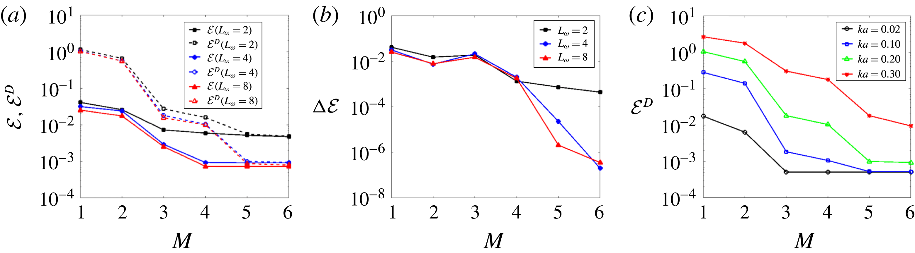
To illustrate the HOR procedure, figure 2(a,b) shows the results of
 ${\mathcal{E}}$
,
 $\unicode[STIX]{x0394}{\mathcal{E}}$
and
 ${\mathcal{E}}^{{\mathcal{D}}}$
as function of
 $L_{\unicode[STIX]{x1D714}}$
and
 $M$
for the reconstruction of Stokes wave with
 $ka=0.20$
. Note that in HOR for each
 $L_{\unicode[STIX]{x1D714}}$
and
 $M$
, once
 $\unicode[STIX]{x1D730}^{(M)}$
is optimized, HOS is simply continued in time to calculate
 ${\mathcal{E}}^{{\mathcal{D}}}$
. We see that for
 $L_{\unicode[STIX]{x1D714}}=2$
, as
 $M$
increases, both
 ${\mathcal{E}}$
and
 ${\mathcal{E}}^{{\mathcal{D}}}$
decrease and at
 $M=6$
,
 $\unicode[STIX]{x0394}{\mathcal{E}}$
is below
 $\tilde{{\mathcal{E}}}$
, but
 ${\mathcal{E}}$
is still larger than
 ${\mathcal{E}}^{\ast }$
, which means further increasing
 $M$
is not effective as the number of free wave components
 $L_{\unicode[STIX]{x1D714}}$
is too small. Thus we increase
 $L_{\unicode[STIX]{x1D714}}$
to 4 and repeat the iteration on
 $M$
. At
 $M=5$
, both
 $\unicode[STIX]{x0394}{\mathcal{E}}<\tilde{{\mathcal{E}}}$
and
 ${\mathcal{E}}<{\mathcal{E}}^{\ast }$
are satisfied and the reconstruction is regarded finished. The results of
 $M=6$
are shown just for comparison. The results of
 $L_{\unicode[STIX]{x1D714}}=8$
are used to confirm
 $L_{\unicode[STIX]{x1D714}}=4$
is sufficient for this case, as the results of
 ${\mathcal{E}}$
and
 ${\mathcal{E}}^{{\mathcal{D}}}$
are quite close for
 $L_{\unicode[STIX]{x1D714}}=4$
and 8. With sufficiently large
 $N$
which we use, convergence of HOR reconstruction is obtained with increasing
 $L_{\unicode[STIX]{x1D714}}$
and
 $M$
.
(a) Reconstruction error
 ${\mathcal{E}}$
, prediction error
 ${\mathcal{E}}^{{\mathcal{D}}}$
and (b)
 $\unicode[STIX]{x0394}{\mathcal{E}}$
as function of
 $M$
in HOR for the reconstruction of Stokes wave with steepness
 $ka=0.20$
using different
 $L_{\unicode[STIX]{x1D714}}$
, and (c)
 ${\mathcal{E}}^{{\mathcal{D}}}$
as function of
 $M$
in HOR for the reconstruction of Stokes waves of different steepness
 $ka$
using
 $L_{\unicode[STIX]{x1D714}}=4$
. For the results shown,
 ${\mathcal{E}}^{\ast }=10^{-3}$
and
 $\tilde{{\mathcal{E}}}={\mathcal{E}}^{\ast }/2$
,
 ${\mathcal{D}}=\{x\in [0,\unicode[STIX]{x1D706}_{0}],t/T=2\}$
and
 ${\mathcal{M}}=\{x=0,t/T\in [0,1]\}$
. For
 $M=1,2$
, analytic wave models are used while for
 $M\geqslant 3$
, HOS model with computational domain
 $x/\unicode[STIX]{x1D706}_{0}\in [-3.5,3,5]$
and
 $N=512$
(corresponding to 1024 data points in space) is used, where
 $\unicode[STIX]{x1D706}_{0}\equiv gT^{2}/(2\unicode[STIX]{x03C0})$
.

Figure 2(a) also shows the relationship between
 ${\mathcal{E}}$
and
 ${\mathcal{E}}^{{\mathcal{D}}}$
. We see that for
 $L_{\unicode[STIX]{x1D714}}=2$
,
 ${\mathcal{E}}$
decreases relatively slowly as
 $M$
increases until
 $\unicode[STIX]{x0394}{\mathcal{E}}$
is less than
 $\tilde{{\mathcal{E}}}$
, while for sufficient
 $L_{\unicode[STIX]{x1D714}}=4$
,
 ${\mathcal{E}}$
decreases rapidly as
 $M$
increases until
 ${\mathcal{E}}$
reaches the prescribed tolerance. It also shows that especially for small value of
 $M$
,
 ${\mathcal{E}}^{{\mathcal{D}}}$
is much larger than
 ${\mathcal{E}}$
. Thus nonlinear effects are especially important in order to forecast the wave field well. For
 $L_{\unicode[STIX]{x1D714}}=4$
,
 ${\mathcal{E}}^{{\mathcal{D}}}$
also decreases rapidly as
 $M$
increases until
 ${\mathcal{E}}<{\mathcal{E}}^{\ast }$
and
 ${\mathcal{E}}^{{\mathcal{D}}}$
is constrained by
 ${\mathcal{E}}$
.
To examine the behaviour of
 ${\mathcal{E}}^{{\mathcal{D}}}$
as
 $M$
increases for different
 $ka$
, figure 2(c) shows the detailed results of
 ${\mathcal{E}}^{{\mathcal{D}}}$
for each case. We see that for all cases with sufficiently large
 $L_{\unicode[STIX]{x1D714}}=4$
,
 ${\mathcal{E}}^{{\mathcal{D}}}$
decreases exponentially as
 $M$
increases until it is constrained by
 ${\mathcal{E}}$
. For given
 $M$
,
 ${\mathcal{E}}^{{\mathcal{D}}}$
grows rapidly as
 $ka$
increases. As the wave becomes steeper, higher order of nonlinearity is needed in order for
 ${\mathcal{E}}^{{\mathcal{D}}}$
to reach the same level of reconstruction accuracy. For example, for
 $ka=0.30$
, we need
 $M=7$
(not shown). Note that HOR can reconstruct Stokes wave with steepness up to the limit of HOS, which is close to 80 % of limited Stokes steepness. We remark again that the Stokes wavelength is unknown, and
 $L_{\unicode[STIX]{x1D714}}=1$
would not in general be sufficient in HOR reconstruction. This is different from classical Stokes expansion where a wave of given fundamental length is expanded to increasingly high order.
3 Results
We illustrate HOR using both synthetic wave fields and laboratory measurements. We consider uni- and multidirectional irregular waves without restrictions on frequency and directional band width. These tests demonstrate the performance of HOR, address the importance of including higher-order nonlinearity in the reconstruction, and assess the usefulness of such nonlinear reconstruction in terms of the space–time domain in which the underlying wave fields can be predicted.
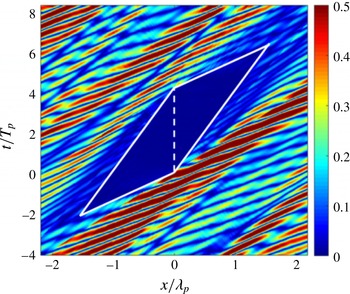
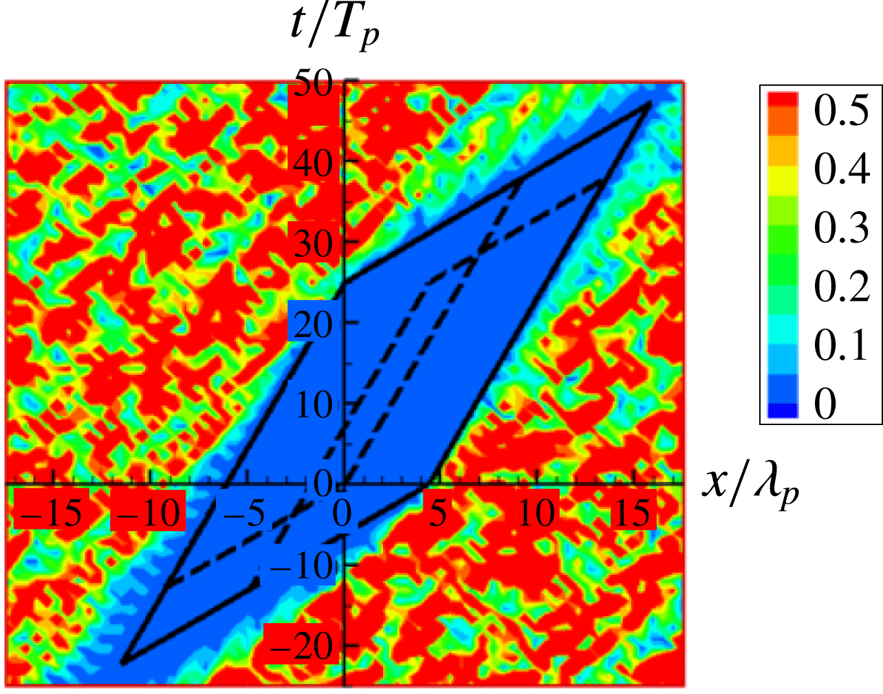
Point-to-point prediction error
 $e(x,t)$
for an unidirectional wave field reconstructed by HOR with
 $L_{\unicode[STIX]{x1D714}}=32$
,
 $M=1$
and
 $N=512$
based on a single point measurement,
 $\unicode[STIX]{x1D701}(x=0,t/T_{p}\in [0,4.17])$
(with peak period
 $T_{p}=12~\text{s}$
, peak wavelength
 $\unicode[STIX]{x1D706}_{p}=227.72~\text{m}$
and effective wave steepness
 $(ka)_{e}=0.04$
). The region enclosed by the white solid line is the linear predictable zone
 ${\mathcal{P}}_{L}$
with maximum
 $x$
–
 $t$
point given by
 $x/\unicode[STIX]{x1D706}_{p}=1.57$
and
 $t/T_{p}=6.42$
and the dashed line indicates the measurement duration and location.

3.1 Reconstruction of unidirectional waves
3.1.1 Synthetic waves with a single point measurement
We consider here reconstruction of unidirectional waves based on a single point measurement. The original wave elevation
 $\tilde{\unicode[STIX]{x1D702}}(x,t)$
is generated by HOS simulation (with
 $M=3$
) from a JONSWAP wave spectrum
 $S(\unicode[STIX]{x1D714})$
with peak-enhancement parameter
 $\unicode[STIX]{x1D6FE}=3.3$
and peak frequency
 $\unicode[STIX]{x1D714}_{p}=0.52~\text{rad}~\text{s}^{-1}$
, propagating in the
 $+x$
direction. We define the effective wave steepness of the irregular waves to be
 $(ka)_{e}\equiv 4\unicode[STIX]{x03C0}\unicode[STIX]{x1D70E}/\unicode[STIX]{x1D706}_{p}$
, where
 $\unicode[STIX]{x1D70E}$
is the root-mean-square of elevation and
 $\unicode[STIX]{x1D706}_{p}$
is the peak wave length. For this example, we choose the wave field with energy being within the frequency band
 $[\unicode[STIX]{x1D714}_{a}=0.7,\unicode[STIX]{x1D714}_{b}=2.0]\unicode[STIX]{x1D714}_{p}$
. Note that in this example, as well as later cases, with
 $\unicode[STIX]{x1D6FE}=3.3$
, the wave field is not narrow banded. We use
 $\unicode[STIX]{x1D701}(t)\equiv \tilde{\unicode[STIX]{x1D702}}(x=0,t)$
, for
 $t/T_{p}\in [0,4.17]$
as the measurement.
As an initial test, we consider a very small
 $(ka)_{e}=0.04$
. Figure 3 displays the point-to-point prediction error
 $e(x,t)\equiv |\unicode[STIX]{x1D702}(x,t)-\tilde{\unicode[STIX]{x1D702}}(x,t)|/\unicode[STIX]{x1D70E}$
in the
 $x$
–
 $t$
domain obtained with HOR which converges with
 $M=1$
,
 $L_{\unicode[STIX]{x1D714}}=32$
(with HOS
 $N=512$
). The contour of
 $e(x,t)$
, say defined by
 $e(x,t)\leqslant {\mathcal{E}}^{\ast }=0.01$
, indicates the region(s) of predictability
 ${\mathcal{P}}$
. In this case, the wave field is approximately linear, and
 ${\mathcal{P}}$
is close to the linear predictable zone
 ${\mathcal{P}}_{L}$
indicated by the parallelogram in figure 3. In this case,
 ${\mathcal{P}}_{L}$
is given by a simple closed-form formula in terms of measurement duration and the wave group velocities at frequencies
 $\unicode[STIX]{x1D714}_{a}$
and
 $\unicode[STIX]{x1D714}_{b}$
, which is presented in Qi et al. (Reference Qi, Wu, Liu and Yue2018). Outside
 ${\mathcal{P}}\approx {\mathcal{P}}_{L}$
, the point-to-point prediction error
 $e(x,t)$
is continuous but increases to
 $O(1)$
within a distance/time of
 $x/\unicode[STIX]{x1D706}_{p}$
,
 $t/T_{p}$
 ${\approx}O(1)$
from
 ${\mathcal{P}}_{L}$
.
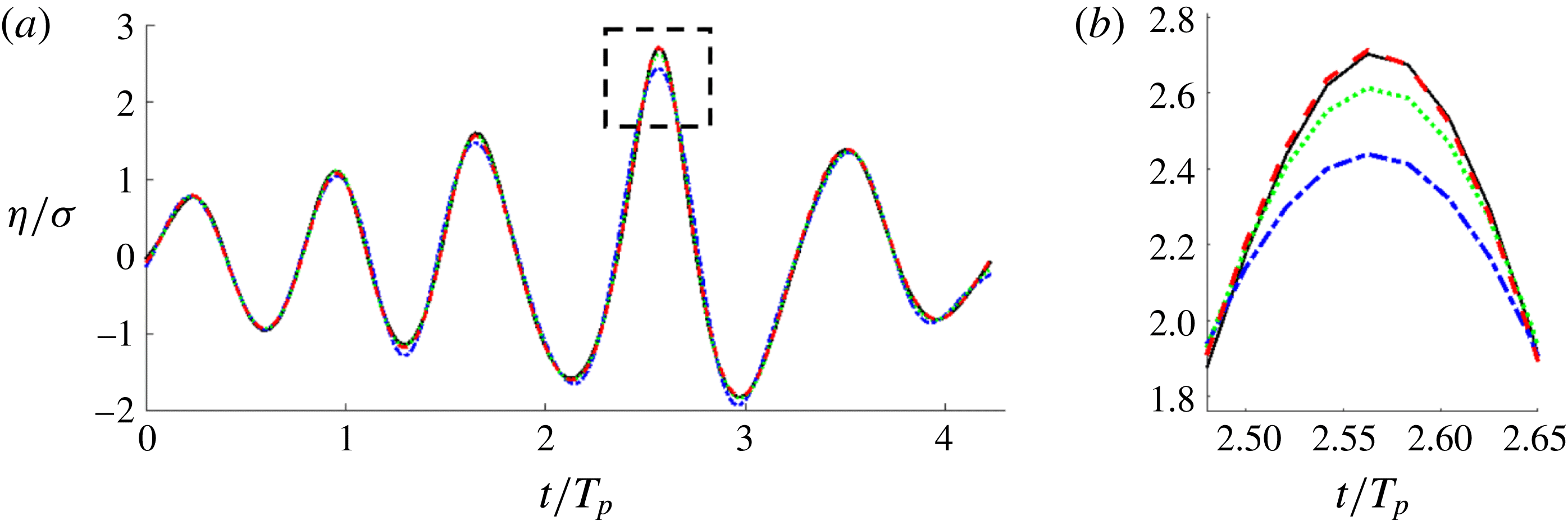
(a) Comparison of the wave elevation histories at the measurement location (
 $x=0$
) from the reconstructed wave fields using HOR with
 $M=1$
(— ⋅ — (blue)),
 $M=2$
(
 $\cdots \cdots$
(green)) and
 $M=3$
(– – – (red)) and the measurement data of the synthetic nonlinear wave field (——), where
 $\unicode[STIX]{x1D70E}$
is the root-mean-square of the measurement elevation. (b) Close up of the comparison around
 $t/T_{p}=2.55$
(enlarged view of the dashed square in (a)). (The effective wave steepness
 $(ka)_{e}=0.11$
).

Point-to-point prediction error
 $e_{(M)}(x,t)$
for the reconstructed wave fields using HOR with (a)
 $M=1$
, (b)
 $M=2$
and (c)
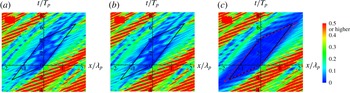
 $M=3$
. Parallelogram region enclosed by the solid line is the linear predictable zone
 ${\mathcal{P}}_{L}$
. The parallelogram region enclosed by the red dash line in (c) is the nonlinear predictable zone
 ${\mathcal{P}}_{S}$
obtained by use of the second-order wave group velocity.

We now consider a realistic case of moderate
 $(ka)_{e}=0.11$
. The JONSWAP spectrum used to generate the high-order (
 $M=3$
) HOS wave field is otherwise the same as before, and the location/duration of the single point elevation measurement
 ${\mathcal{M}}$
is the same as before.
We apply nonlinear HOR reconstruction with
 $N=512$
in HOS, obtaining convergent HOR parameters of
 $L_{\unicode[STIX]{x1D714}}=32$
and
 $M=3$
for specified reconstruction tolerance
 ${\mathcal{E}}^{\ast }=0.01$
. Figure 4 plots the direct comparison of the wave elevation history at the measurement location between the given data and those of the reconstructed wave fields with
 $M=1,2,3$
. Figure 5 shows the point-to-point prediction error
 $e_{(M)}(x,t)\equiv |\unicode[STIX]{x1D702}_{(M)}(x,t)-\tilde{\unicode[STIX]{x1D702}}(x,t)|/\unicode[STIX]{x1D70E}$
for
 $M=1,2,3$
in the
 $x$
–
 $t$
domain. As a reference, the linear predictable zone
 ${\mathcal{P}}_{L}$
is also indicated. Note that for this case HOR converges with
 $M=3$
. We confirm (not shown) that point-to-point prediction errors
 $e_{(3)}$
and
 $e_{(4)}$
are graphically indistinguishable.
From figure 4, we see that the reconstructed wave elevation with
 $M=1,2,3$
all recover the original data well for most of the measurement time except at wave crests and troughs, where reconstruction with
 $M=1$
and 2 have an error of up to 18 and 5 % respectively. Figure 5 further shows that point-to-point prediction error
 $e_{(3)}$
within
 ${\mathcal{P}}_{L}$
is much smaller than
 $e_{(1)}$
and
 $e_{(2)}$
. Specifically, for this example, the maximum
 $e_{(3)}$
inside
 ${\mathcal{P}}_{L}$
is less than 3 % while
 $e_{(1)}$
and
 $e_{(2)}$
can be as large as 20 %.
 ${\mathcal{E}}^{{\mathcal{P}}_{L}}$
for
 $M=1,2,3$
are 8.5, 7.9 and 1.3 %, respectively. These results indicate that inclusion of high-order wave effects is of importance in the reconstruction of the nonlinear wave field within the whole predictable zone.
Note that in figure 5(c) where the reconstruction converges, the actual (nonlinear) predictable zone
 ${\mathcal{P}}_{NL}$
, which corresponds to approximately the blue region where point-to-point prediction error
 $e(x,t)\leqslant e_{0}=0.01$
, is actually larger than
 ${\mathcal{P}}_{L}$
due to the nonlinear effects. Since there is no closed-form expression for the wave field based on fully nonlinear wave theory, it is hard to derive the closed-form expression for
 ${\mathcal{P}}_{NL}$
. We provide an estimate of
 ${\mathcal{P}}_{NL}$
by simply extending the linear predictable zone theory to include nonlinear wave effects on the wave group velocity. In nonlinear wave-field evolution, the wave dispersion relation can be affected by resonant wave–wave interactions, wave group interactions, and bound wave effects depending on the time/space scale of the problem considered. For short-time phase-resolved wave-field reconstruction, the second-order bound wave effects are of importance.
The group velocity of each wave component calculated from the second-order nonlinear dispersion relation (Longuet-Higgins Reference Longuet-Higgins1962; Hogan, Gruman & Stiassnie Reference Hogan, Gruman and Stiassnie1988) (see details in appendix B) is generally larger than the linear one. In this example, the linear dispersion relation gives the minimum (maximum) group velocity of
 $4.62~\text{m}~\text{s}^{-1}$
(
 $13.61~\text{m}~\text{s}^{-1}$
), while the second-order dispersion relation gives
 $5.15~\text{m}~\text{s}^{-1}$
(
 $13.93~\text{m}~\text{s}^{-1}$
). As a result, the size of predictable zone becomes larger when second-order effects are accounted for, as shown in figure 5(c) where a quantitative comparison between the linear and second-order predictable zones is made. Hereafter we use
 ${\mathcal{P}}_{S}$
to denote the nonlinear predictable zone considering the second-order effects. We can see that in this example
 ${\mathcal{P}}_{S}$
estimates
 ${\mathcal{P}}_{NL}$
better than
 ${\mathcal{P}}_{L}$
.
From the HOR reconstructed wave fields with different
 $(ka)_{e}$
, and by looking at the converged
 $e(x,t)$
we estimate that
 ${\mathcal{P}}_{NL}-{\mathcal{P}}_{L}$
increases approximately linearly with increasing
 $(ka)_{e}$
. This can be shown more clearly by using
 ${\mathcal{P}}_{S}$
to estimate
 ${\mathcal{P}}_{NL}$
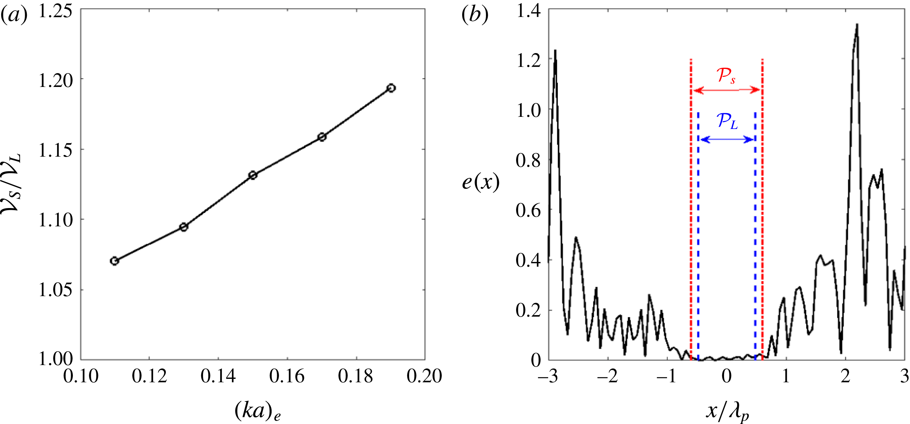
. Figure 6(a) plots the ratio of the volume of
 ${\mathcal{P}}_{S}$
and
 ${\mathcal{P}}_{L}$
, denoted as
 ${\mathcal{V}}_{S}$
and
 ${\mathcal{V}}_{L}$
respectively, as a function of
 $(ka)_{e}$
. It shows
 ${\mathcal{V}}_{S}/{\mathcal{V}}_{L}$
increases approximately linearly as
 $(ka)_{e}$
increases. We point out that for an irregular wave field with effective wave steepness of 0.19, the local wave steepness in the wave field can be as large as 1.0 in many places. In this case,
 ${\mathcal{V}}_{S}$
is greater than
 ${\mathcal{V}}_{L}$
by about 20 %. Figure 6(b) further shows the distribution of point-to-point prediction error
 $e(x,t)$
at time
 $t/T_{p}=2.08$
(the midpoint of measurement duration) for the case of
 $(ka)_{e}=0.19$
, when the reconstruction converges using HOR with
 $M=4$
. At this time,
 ${\mathcal{P}}_{S}$
is larger than
 ${\mathcal{P}}_{L}$
for approximately 14 %. This difference is most significant near the starting and ending time of the predictable zone, which leads to a total volume difference of 20 %.
Based on these results, we see that for (very) small wave steepness
 $(ka)_{e}\rightarrow 0$
,
 ${\mathcal{P}}_{NL}\rightarrow {\mathcal{P}}_{L}$
. As wave steepness increases,
 ${\mathcal{P}}_{NL}$
contains and is greater than
 ${\mathcal{P}}_{L}$
(
 ${\mathcal{P}}_{NL}\supseteq {\mathcal{P}}_{L}$
), with
 ${\mathcal{P}}_{NL}-{\mathcal{P}}_{L}$
increasing approximately linearly with increasing
 $(ka)_{e}$
. We note that
 $P_{NL}$
depends on the value of the acceptable error
 $e_{0}$
, within which the point-to-point error in the predicted wave field
 $e(x,t)\leqslant e_{0}$
. These are seen in the contour plots of
 $e(x,t)$
(figures 5 and 6
b). As
 $e_{0}$
(and reconstruction error
 ${\mathcal{E}}^{\ast }\leqslant e_{0}$
) decreases,
 $P_{NL}$
decreases as expected, but our results show that
 $P_{NL}$
remains greater than
 $P_{L}$
. This is partly due to the greater group velocity with increasing nonlinearity as discussed above.
(a) The ratio of the volume
 ${\mathcal{V}}_{S}/{\mathcal{V}}_{L}$
of second-order and linear predictable zones as a function of the effective wave steepness
 $(ka)_{e}$
(other spectrum parameters are kept the same in the generation of synthetic high-order (
 $M=5$
) HOS wave fields). (b) Distribution of point-to-point prediction error
 $e(x,t)$
at
 $t/T_{p}=2.08$
for wave field with
 $(ka)_{e}=0.19$
when the reconstruction converges using HOR with
 $M=4$
, where
 ${\mathcal{P}}_{L}$
and
 ${\mathcal{P}}_{S}$
indicate the linearized and nonlinear (considering second-order effects) predictable zones.

We note that HOR/HOS provides not only wave elevation for comparison to measurements, but all other wave kinematics such as velocities. We will discuss the importance of including higher-order effects in the reconstruction of wave kinematics in § 3.1.3.
As further illustration, we use synthetic high-order (
 $M=5$
) HOS wave fields of different wave steepness, which are generated by the same JONSWAP spectrum as above, to validate HOR and examine the convergence of reconstruction. The location/duration of the single point elevation measurement
 ${\mathcal{M}}$
is the same as before. Table 1 shows the prediction error
 ${\mathcal{E}}^{{\mathcal{P}}}$
as a function of
 $M$
in HOR for different wave steepness, where
 ${\mathcal{P}}_{S}$
is used as an estimate for actual
 ${\mathcal{P}}$
. It further confirms that as the wave steepness increases, higher order of reconstruction is needed in order for the prediction error to reach the same level of reconstruction tolerance. Based on our tests, the reconstructed wave field always converges to the underlying wave field within the predictable zone for wave steepness up to the limit of HOS simulation.
Point-to-point prediction error
 $e(x,t)$
for a unidirectional wave field (
 $(ka)_{e}=0.03$
) reconstructed by HOR with
 $L_{\unicode[STIX]{x1D714}}=32$
,
 $M=1$
, and
 $N=512$
based on two point measurements (at
 $\unicode[STIX]{x1D709}_{1}/\unicode[STIX]{x1D706}_{p}=0$
and
 $\unicode[STIX]{x1D709}_{2}/\unicode[STIX]{x1D706}_{p}=4.39$
with time duration
 $t/T_{p}\in [0,25]$
). Parallelogram region enclosed by the white solid lines is the linear predictable zone
 ${\mathcal{P}}_{L}$
based on the combination of two measurements. Parallelogram regions enclosed by dashed line and dotted line are the linear predictable zones associated with each individual measurement.

Prediction error
 ${\mathcal{E}}^{{\mathcal{P}}}$
as function of
 $M$
in HOR for the reconstruction of the synthetic unidirectional high-order (
 $M=5$
) HOS wave fields with different
 $(ka)_{e}$
based on a single point measurement.
 $L_{\unicode[STIX]{x1D714}}=32$
,
 $N=512$
,
 ${\mathcal{E}}^{\ast }=0.01$
and
 $\tilde{{\mathcal{E}}}={\mathcal{E}}^{\ast }/2$
are used in HOR. The symbol ‘—’ means
 ${\mathcal{E}}^{{\mathcal{P}}}(M)\simeq {\mathcal{E}}^{{\mathcal{P}}}(M-1)$
.

3.1.2 Synthetic waves with multiple point measurements
We now consider reconstruction of synthetic unidirectional wave fields based on multiple point measurements. The wave fields with
 $(ka)_{e}=0.03$
and 0.12 are generated from a JONSWAP spectrum
 $S(\unicode[STIX]{x1D714})$
using the same parameters as in § 3.1.1 by HOS simulations with
 $M=3$
. Without loss of generality, we consider two point measurements at
 $\unicode[STIX]{x1D709}_{1}/\unicode[STIX]{x1D706}_{p}=0$
and
 $\unicode[STIX]{x1D709}_{2}/\unicode[STIX]{x1D706}_{p}=4.39$
. The data for both measurements are taken in the duration of
 $t/T_{p}\in [0,25]$
.
For the wave field of small wave steepness
 $(ka)_{e}=0.03$
, the HOR reconstruction with
 $L_{\unicode[STIX]{x1D714}}=32$
,
 $M=1$
, and
 $N=512$
converges. Figure 7 shows
 $e(x,t)$
in
 $x$
–
 $t$
, where
 ${\mathcal{P}}_{L}$
is indicated. In this multiple measurements case,
 ${\mathcal{P}}_{L}$
is obtained by first calculating the union of predictable zones from each measurement for each wave frequency component in the wave field, then determining the intersection of the predictable zones of all wave frequency components in the wave field (Qi et al.
Reference Qi, Wu, Liu and Yue2018). It confirms again that for very small wave steepness,
 ${\mathcal{P}}_{L}$
estimates the actual predictable zone accurately, which corresponds to the dark blue region where
 $e(x,t)\leqslant 0.01$
. We see that outside
 ${\mathcal{P}}_{L}$
,
 $e(x,t)$
is continuous but increases to
 $O(1)$
within a distance/time of
 $x/\unicode[STIX]{x1D706}_{p}$
,
 $t/T_{p}$
 ${\approx}O(1)$
from
 ${\mathcal{P}}_{L}$
.
For the wave field of large wave steepness
 $(ka)_{e}=0.12$
, we use
 $N=1024$
and obtain
 $L_{\unicode[STIX]{x1D714}}=60$
and
 $M=3$
in order for
 ${\mathcal{E}}<{\mathcal{E}}^{\ast }=0.01$
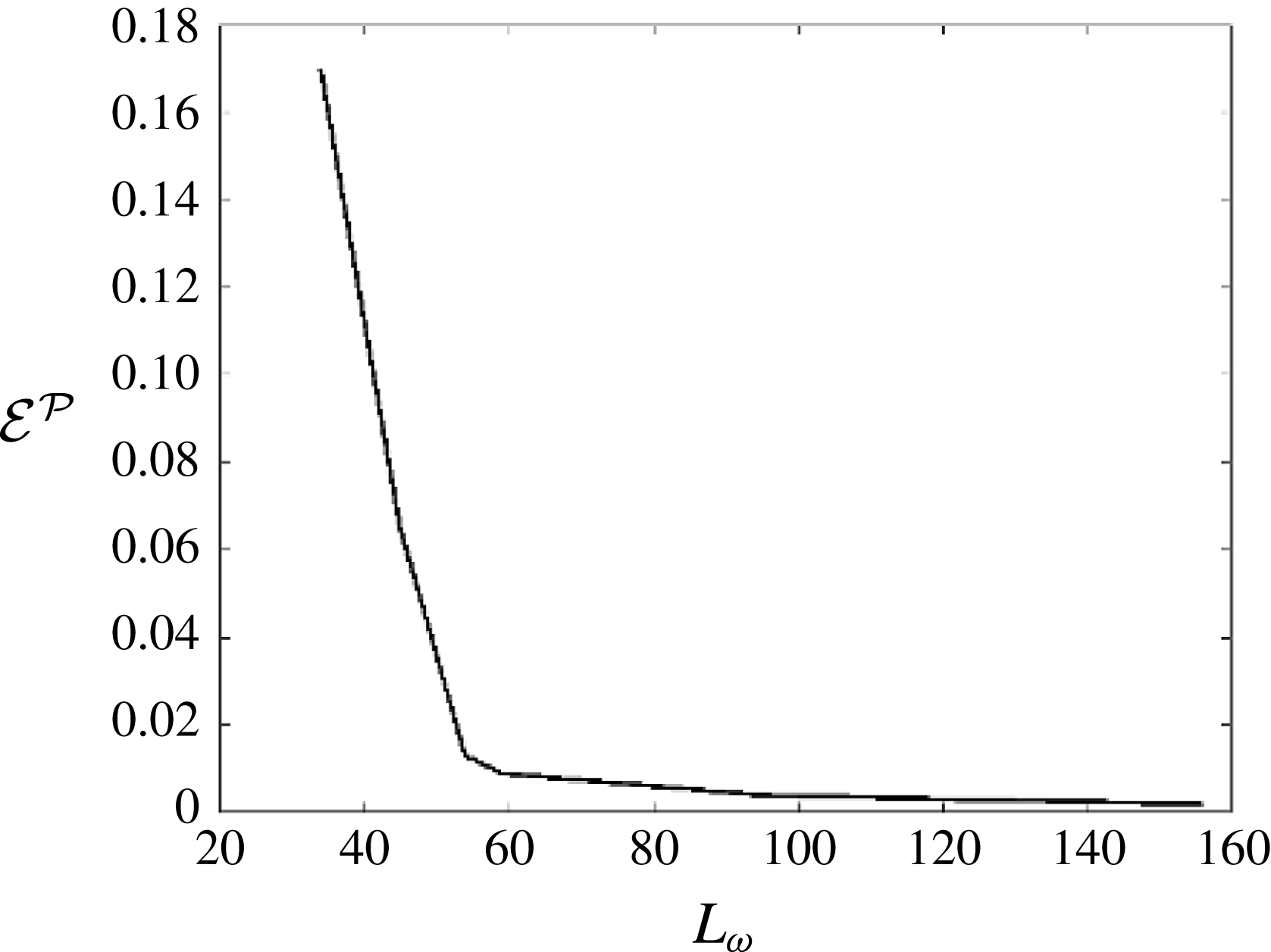
. To illustrate the effect of
 $L_{\unicode[STIX]{x1D714}}$
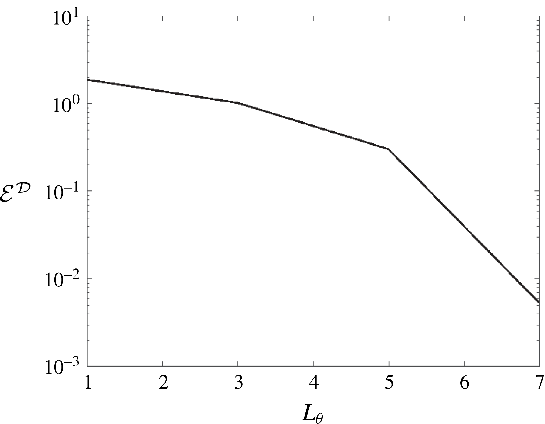
on the prediction, figure 8 shows the prediction error
 ${\mathcal{E}}^{{\mathcal{P}}}$
using fixed
 $M=3$
as a function of
 $L_{\unicode[STIX]{x1D714}}$
, where
 ${\mathcal{P}}_{S}$
is used to estimate the actual
 ${\mathcal{P}}$
. As
 $L_{\unicode[STIX]{x1D714}}$
increases,
 ${\mathcal{E}}^{{\mathcal{P}}}$
first decreases abruptly, and then after a turning point
 ${L_{\unicode[STIX]{x1D714}}}^{c}\sim 60$
,
 ${\mathcal{E}}^{{\mathcal{P}}}$
decreases slowly and converges. In this case,
 ${\mathcal{E}}^{{\mathcal{P}}}$
is approximately
 $1\,\%$
for
 $L_{\unicode[STIX]{x1D714}}=60$
which is the same level as the reconstruction tolerance, and
 $L_{\unicode[STIX]{x1D714}}=60$
is selected as the optimal
 $L_{\unicode[STIX]{x1D714}}$
by HOR.
The prediction error (
 ${\mathcal{E}}^{{\mathcal{P}}}$
) as a function of
 $L_{\unicode[STIX]{x1D714}}$
used in HOR with fixed
 $M=3$
for the reconstruction of synthetic nonlinear wave field (
 $(ka)_{e}=0.12$
) based on two point measurements.

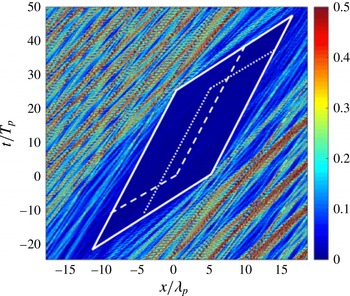
Figure 9 displays point-to-point prediction error
 $e(x,t)$
in
 $x$
–
 $t$
for the nonlinear reconstruction.
 ${\mathcal{P}}_{S}$
is also indicated to estimate the actual predictable zone, which corresponds to the blue region where
 $e(x,t)\leqslant 0.01$
. Outside
 ${\mathcal{P}}_{S}$
,
 $e(x,t)$
increases to
 $O(1)$
within a distance/time of
 $x/\unicode[STIX]{x1D706}_{p}$
,
 $t/T_{p}$
 ${\approx}O(1)$
from
 ${\mathcal{P}}_{S}$
. The results in figures 7 and 9 both confirm the theoretical result that the predictable zone based on the combination of two point measurements (within a certain distance) is larger than the simple union of the predictable zones associated with each individual measurement.
Point-to-point prediction error
 $e(x,t)$
in the numerically reconstructed nonlinear wave field (
 $(ka)_{e}=0.12$
) based on two point measurements (at
 $\unicode[STIX]{x1D709}_{1}/\unicode[STIX]{x1D706}_{p}=0$
and
 $\unicode[STIX]{x1D709}_{2}/\unicode[STIX]{x1D706}_{p}=4.39$
with time duration
 $t/T_{p}\in [0,25]$
). Parallelogram region enclosed by solid lines is the nonlinear predictable zone (considering second-order group velocities)
 ${\mathcal{P}}_{S}$
based on the combination of two measurements. Parallelogram regions by dashed lines are the predictable zones associated with each individual measurement.

3.1.3 Comparison to two-dimensional wave tank experiments
So far, we have considered theoretical Stokes waves and synthetic wave fields. It is important to demonstrate HOR and verify the predictable zone theory for realistic physical wave field which contains measurement errors. Here we first consider two-dimensional experiments conducted in the narrow wave tank at Texas A&M University. Later in § 3.2.3 we discuss a three-dimensional wave-basin experiment.
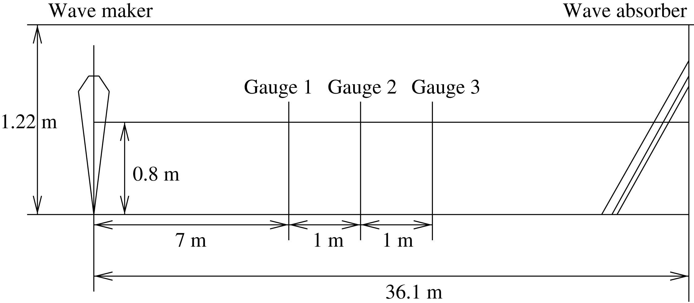
(i) Set-up of experiment. The glass-walled flume has a length of 36.1 m, a width of 0.91 m and a height of 1.22 m and is equipped with a permeable wave absorbing beach at downstream. Wave generation is provided by a dry-back, hinged flap wavemaker capable of producing regular and irregular waves with period ranging from 0.25 to 4.0 s and maximum height of 0.254 m. The set-up is shown schematically in figure 10, where
 $x$
is the horizontal coordinate positive in the direction of wave propagation with
 $x=0$
at the wavemaker and
 $z$
positive upwards.
Experimental set-up in the narrow wave tank at Texas A&M University.

A JONSWAP spectrum with
 $\unicode[STIX]{x1D6FE}=1$
(Pierson–Moskowitz spectrum) and peak wavelength
 $\unicode[STIX]{x1D706}_{p}=1.25~\text{m}$
is used for the generation of irregular waves. The water depth in the tank is
 $h=0.80~\text{m}$
. To investigate the importance of nonlinear effects, two irregular wave trains with significant wave heights of
 $H_{s}=0.04~\text{m}$
and 0.09 m are generated. The free-surface elevation is recorded using resistant-type surface-piercing wave gauges at three locations
 $x=7.0$
, 8.0, and 9.0 m. The wave kinematics are measured using a laser Doppler velocimeter (LDV) system at the location
 $x=8.0~\text{m}$
for seven vertical positions below the still water level (SWL) and two vertical positions above the SWL. The optic cable LDV measures the three velocity components simultaneously with high spatial resolution. As a non-intrusive measurement, the LDV measurement has been proved to be of high accuracy in other experiments (e.g. Skjelbreia Reference Skjelbreia1987; Agrawal & Aubrey Reference Agrawal and Aubrey1992). For both tests, the time series of wave elevation and velocity are recorded for about 250 s.
(ii) Wave elevation comparison. For the two irregular wave trains tested, the effective wave steepness are
 $(ka)_{e}=0.10$
and 0.23. To reconstruct these wave fields, we choose partial records at
 $x=8.0~\text{m}$
which contain the steepest local waves. Specifically, for the case of
 $(ka)_{e}=0.10$
, we use the elevation record in the duration of
 $112.24~\text{s}\leqslant t\leqslant 118.20~\text{s}$
as the given measurement. For the case of
 $(ka)_{e}=0.23$
, the record in the duration of
 $116.75~\text{s}\leqslant t\leqslant 124.88~\text{s}$
is used. In both cases, the record contains 7–8 dominant wave periods. In wave reconstruction, we finally obtain
 $L_{\unicode[STIX]{x1D714}}=22$
, and
 $M=3$
for
 ${\mathcal{E}}<{\mathcal{E}}^{\ast }=0.01$
. For the HOS simulation, we use
 $N=512$
. The computation domain contains about 50 dominant waves and about 500 shortest waves.
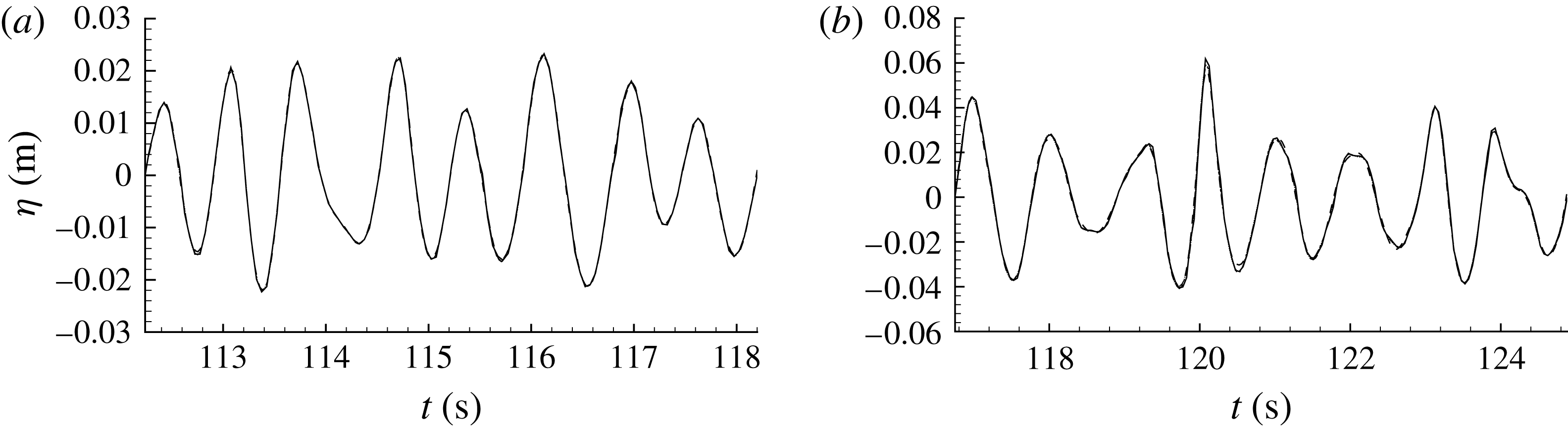
Comparison of reconstructed versus experimental free-surface elevation at the measurement location as a function of time for irregular wave trains with (a)
 $(ka)_{e}=0.10$
; and (b)
 $(ka)_{e}=0.23$
. Plotted are the experimental record (——), linear reconstruction (— ⋅ —), second-order reconstruction (
 $\cdots \cdots$
), and third-order reconstruction (– – –) based on HOS simulations (with
 $N=512$
).

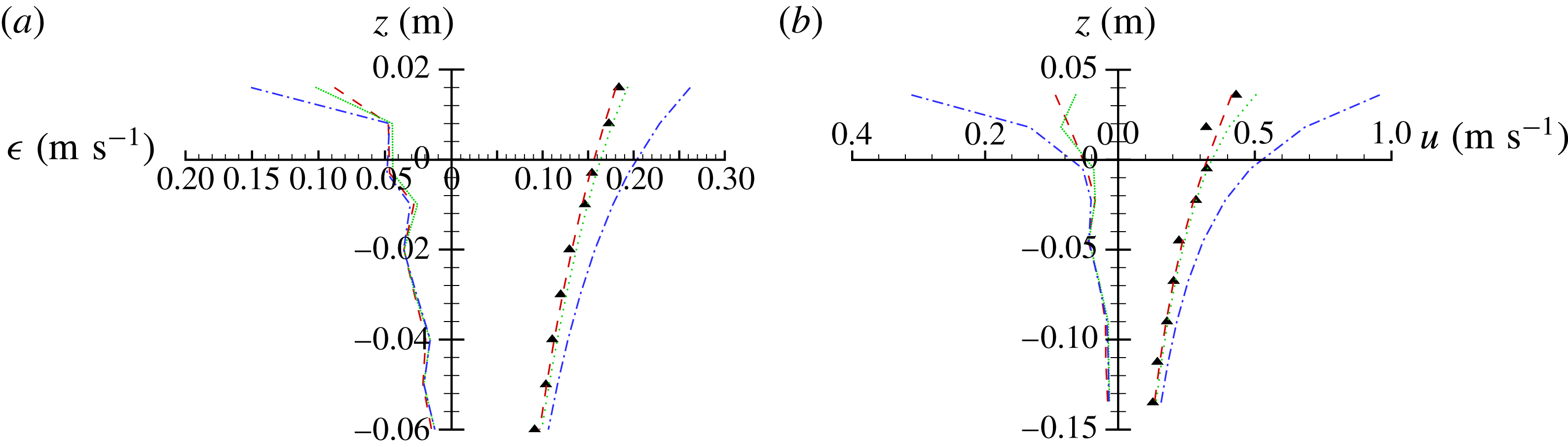
Comparison of reconstructed versus experimental horizontal velocity along the depth under wave crest at measurement location (
 $x=8.0~\text{m}$
): experimental measurement (▴),
 $M=1$
prediction (— ⋅ — (blue)),
 $M=2$
prediction (
 $\cdots \cdots$
(green)) and
 $M=3$
prediction (– – – (red)) based on HOS simulation with
 $N=512$
spectral modes. (a) Plots the time averaged errors of reconstructed velocity with different nonlinear wave models. (b) Shows the result for the horizontal velocity profile at (a) time
 $t=114.725~\text{s}$
for
 $(ka)_{e}=0.10$
, and (b)
 $t=120.075~\text{s}$
for
 $(ka)_{e}=0.23$
.

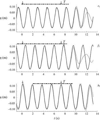
Figure 11 shows the comparison of the wave elevation history at the measurement location between the measurement and the reconstruction obtained using the linear, second- and third-order wave models. It is seen that the reconstructed wave records all agree well with the experimental data.
(iii) Wave kinematics comparison. Although the reconstructed wave fields with the use of linear, second- and third-order wave models all match the wave elevation record at the measurement location, the spatial wave profiles and detailed wave kinematics in these wave fields should differ owing to the effects of wave nonlinearity. We here investigate the importance of the inclusion of wave nonlinearity in the reconstruction of wave kinematics.
Figure 12 shows the comparison of the horizontal velocity between the reconstruction and experimental data. Plotted are the instantaneous vertical variation of the horizontal velocity at measurement location (
 $x=8.0~\text{m}$
) under the wave crest for two different wave steepness
 $(ka)_{e}=0.10$
and
 $(ka)_{e}=0.23$
. Note that, consistent with HOS, the nonlinear velocities near the mean free surface are evaluated using Taylor series expansions up to order
 $M$
(for details, see Wu Reference Wu2004). It is seen that the third-order nonlinear reconstruction (
 $M=3$
) agrees well with the measurement for both cases while the linear and second-order reconstructions largely overestimate the velocity especially in the region near the free surface. The fourth-order reconstruction is also obtained but not shown in the figure since they are very close to the third-order results. Specifically, for the small wave steepness case (
 $(ka)_{e}=0.10$
), the second-order theory provides a proper reconstruction while the linear theory over-predicts the velocity by approximately 40 % near the free surface. As the wave steepness increases to
 $(ka)_{e}=0.23$
, the second-order theory over-predicts the velocity by approximately 25 % and the over-prediction by the linear theory increases to approximately 150 % near the free surface. Note that the plots do not show the velocity profiles up to the exact free surface because the experimental measurement at the free surface cannot be reliably obtained. For
 $(ka)_{e}=0.23$
(or 0.10), the crest wave elevation reaches 0.061 m (or 0.022 m) at time
 $t=120.075~\text{s}$
(or 114.725 s) (cf. figure 11). From the trend of the velocity profiles, it is seen that the linear and second-order theories will overestimate the horizontal velocity even more at the free surface.
The overestimation of the velocity by the low-order theories depends on the time. To account for this, we define an averaged error of the horizontal velocity as
 $$\begin{eqnarray}\unicode[STIX]{x1D716}_{u}(z)=\left\{\frac{1}{T}\int _{0}^{T}[u(\unicode[STIX]{x1D743}_{j},z,t)-\tilde{u} (\unicode[STIX]{x1D743}_{j},z,t)]^{2}\,\text{d}t\right\}^{1/2},\end{eqnarray}$$
where
 $u$
is the horizontal velocity computed in wave reconstruction and
 $\tilde{u}$
is the experimental measurement. This is also shown in figure 12 as a function of the vertical coordinate
 $z$
. It indicates that in general the linear wave model overestimates the horizontal velocity above the mean water level although below the mean water level the difference is small for three different wave models.
Based on these comparisons, we see that although all three wave models can reconstruct the wave elevation record very well, other kinematics of the reconstructed wave fields may differ significantly depending on the wave steepness. The first- and second-order theories obtain an appropriate reconstruction of a wave field when the steepness is small. For moderately steep waves, the higher-order nonlinear wave modelling needs to be applied in order to properly reconstruct both the wave elevation and other kinematics of the wave field. One consequence of the velocity reconstruction is for the determination of the wave dynamics that is of significance in practical applications such as the determination of the hydrodynamic wave force on an object.
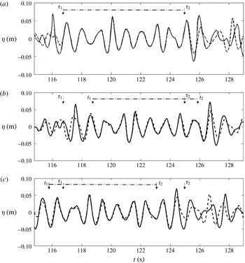
Comparison of the wave elevation histories in the reconstructed wave field (with
 $(ka)_{e}=0.23$
) with experimental measurements at locations of (a)
 $x=8.0~\text{m}$
, (b)
 $x=9.0~\text{m}$
and (c)
 $x=7.0~\text{m}$
. Plotted are the experimental measurements (——) and nonlinear (
 $M=3$
) wave reconstruction (– – –). The dashdot line (— ⋅ —) indicates the predictable time duration at each location, predicted by the linear predictable zone theory.
 $[\unicode[STIX]{x1D70F}_{1},\unicode[STIX]{x1D70F}_{2}]$
represents the measurement time duration at
 $x=8.0~\text{m}$
, where
 $\unicode[STIX]{x1D70F}_{1}=116.75~\text{s}$
and
 $\unicode[STIX]{x1D70F}_{2}=124.88~\text{s}$
. In (a),
 $[\unicode[STIX]{x1D70F}_{1},\unicode[STIX]{x1D70F}_{2}]$
is also the predictable time duration. In (b), wave forecast for
 $t\in [\unicode[STIX]{x1D70F}_{2},t_{2}]$
is obtained, and the prediction error
 ${\mathcal{E}}^{{\mathcal{D}}}=10.29\,\%$
, where
 ${\mathcal{D}}$
corresponds to the predictable time duration
 $[t_{1},t_{2}]$
at this location, with
 $t_{1}=118.79~\text{s}$
and
 $t_{2}=125.90~\text{s}$
. In (c), wave hindcast for
 $t\in [t_{1},\unicode[STIX]{x1D70F}_{1}]$
is obtained, and the prediction error
 ${\mathcal{E}}^{{\mathcal{D}}}=10.95\,\%$
, where
 ${\mathcal{D}}$
corresponds to
 $[t_{1},t_{2}]$
with
 $t_{1}=115.73~\text{s}$
and
 $t_{2}=122.84~\text{s}$
.

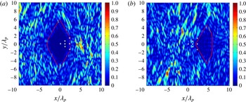
Point-to-point prediction error
 $e(\boldsymbol{x},t)$
for the reconstruction of the multidirectional nonlinear wave field based on seven point measurements at time (a)
 $t/T_{p}=0$
and (b)
 $t/T_{p}=11$
. The measurements are located at
 $(x/\unicode[STIX]{x1D706}_{p},y/\unicode[STIX]{x1D706}_{p})=(0,0)$
,
 $(1.2,0)$
,
 $(1.2,0.8)$
,
 $(1.2,-0.8)$
,
 $(2.4,0)$
,
 $(2.4,1.6)$
,
 $(2.4,-1.6)$
with the same measurement time duration
 $t/T_{p}\in [0,10]$
, where
 $\unicode[STIX]{x1D706}_{p}=25~\text{m}$
and
 $T_{p}=4~\text{s}$
. The regions encircled by red lines are the linear predictable zones
 ${\mathcal{P}}_{L}$
. The bullets denote the measurement locations.

The above results indicate that although all three wave models (
 $M=1,2,3$
) reconstruct the wave elevation record very well, the third-order nonlinear reconstruction regenerates the wave kinematics much better than the lower-order results, especially for steep waves. To understand why the lower-order reconstructions cannot properly regenerate the wave kinematics, we consider a nonlinear Stokes wave of frequency
 $\unicode[STIX]{x1D714}$
. From the Fourier transform of time record of elevation, we shall obtain non-zero amplitudes for all harmonics with frequencies
 $\unicode[STIX]{x1D714},2\unicode[STIX]{x1D714},\ldots ,$
due to the presence of locked waves. In linear wave reconstruction, all high harmonic components are treated as free waves. Unlike free waves, wavenumbers and associated frequencies of the locked waves do not satisfy the dispersion relation. Thus, the resulting reconstructed wave kinematics are incorrect. The wave kinematics, particularly near the free surface, are overestimated since the wavenumbers of the locked waves are amplified when they are incorrectly treated as free waves. The second-order reconstruction improves the accuracy of the reconstructed wave kinematics as it takes into account the second-order locked waves. This is consistent with the findings of Fedele et al. (Reference Fedele, Brennan, De León, Dudley and Dias2016) for ocean waves. As wave steepness increases, however, the second-order reconstruction may not be sufficiently effective. In this case, higher-order reconstruction is needed.
(iv) Forecast of the reconstructed wave field. The predictable zone theory in Qi et al. (Reference Qi, Wu, Liu and Yue2018) indicates that the wave field at downstream (upstream) of the probe can be forecasted (hindcasted). To verify this theory, the wave elevations at both downstream and upstream of the measurement used in wave reconstruction,
 $x=9.0$
and 7.0 m are also measured in the experiment. We compare these measurements with the predictions based on the single point measurement at
 $x=8.0~\text{m}$
. Figure 13 shows the comparisons of the wave elevations at
 $x=8.0$
, 9.0 and 7.0 m for the case of
 $(ka)_{e}=0.23$
.
We apply Fourier analysis on the measurement data and find that the wave energy is mainly contained in the frequency range
 $\unicode[STIX]{x1D714}\in [5,10]~\text{rad}~\text{s}^{-1}$
. Note that for this physical experiment, the underlying wave field is unknown and thus the actual nonlinear predictable zone
 ${\mathcal{P}}_{NL}$
cannot be obtained by comparing the converged reconstructed field with the underlying one. In this case,
 ${\mathcal{P}}_{L}$
provides a conservative estimate for
 ${\mathcal{P}}_{NL}$
. From the linear predictable zone theory, we derive that at
 $x=8.0~\text{m}$
, the predictable time duration is the same as the measurement duration (
 $t\in [116.75,124.88]~\text{s}$
). At
 $x=9.0~\text{m}$
, the wave motion can be predicted for
 $t\in [118.79,125.90]~\text{s}$
, in which
 $t\in [124.88,125.90]~\text{s}$
corresponds to forecast. Figure 13(b) shows that the prediction agrees well with the measurement for a duration a little longer than [118.79, 125.90] s, as
 ${\mathcal{P}}_{NL}$
is a little larger than
 ${\mathcal{P}}_{L}$
. Outside the predictable time duration, the error increases rapidly with evolution time. These confirm the theoretical linear predictable zone based on a single point measurement.
The linear predictable zone theory also indicates that at
 $x=7.0~\text{m}$
, the wave motion can be predicted for
 $t\in [115.73,122.84]~\text{s}$
, in which
 $t\in [115.73,116.75]~\text{s}$
corresponds to hindcast. The satisfactory comparison between the measurement and prediction for a duration of a little larger than [115.73, 122.84] s, shown in figure 13(c) further confirms the predictable zone theory.
3.2 Reconstruction of multidirectional waves
3.2.1 Synthetic waves with multiple point measurements
We consider reconstruction of a synthetic multidirectional nonlinear wave field based on multiple point measurements. The wave field is generated by the HOS simulation (with
 $M=3$
) from a directional JONSWAP spectrum
 $S(\unicode[STIX]{x1D714},\unicode[STIX]{x1D703})=S(\unicode[STIX]{x1D714})D(\unicode[STIX]{x1D703})$
with
 $\unicode[STIX]{x1D6FE}=3.3$
,
 $\unicode[STIX]{x1D714}_{p}=1.57~\text{rad}~\text{s}^{-1}$
,
 $(ka)_{e}=0.13$
,
 $\unicode[STIX]{x1D6FA}=[0.32,1.6]\unicode[STIX]{x1D714}_{p}$
and directional spreading angle
 $\unicode[STIX]{x1D703}\in [-\unicode[STIX]{x03C0}/6,\unicode[STIX]{x03C0}/6]$
. The angular spreading function takes a form of
 $D(\unicode[STIX]{x1D703})=\cos (\unicode[STIX]{x03C0}\unicode[STIX]{x1D703}/(2\unicode[STIX]{x1D6E9}_{0}))^{2}/\unicode[STIX]{x1D6E9}_{0}$
, where
 $\unicode[STIX]{x1D6E9}_{0}=\unicode[STIX]{x03C0}/6$
. Seven point measurements are placed at fixed locations (see figure 14) with same measurement time duration
 $t/T_{p}\in [0,10]$
. In the reconstruction, we use
 $N=1024\times 1024$
(the final results are unaffected varying these) for HOS simulations and we obtain
 $L_{\unicode[STIX]{x1D714}}=40$
,
 $L_{\unicode[STIX]{x1D703}}=7$
and
 $M=3$
for
 ${\mathcal{E}}<{\mathcal{E}}^{\ast }=0.01$
. Figure 14 shows point-to-point prediction error
 $e(\boldsymbol{x},t)$
at two representative time
 $t/T_{p}=0$
(reconstruction) and 11 (forecast). For simplicity,
 ${\mathcal{P}}_{L}$
is also indicated as an estimate of
 ${\mathcal{P}}_{NL}$
. In this multidirectional wave case,
 ${\mathcal{P}}_{L}$
is the intersection of the predictable zones in each wave propagation direction in the wave field (Qi et al.
Reference Qi, Wu, Liu and Yue2018). Excellent agreement between the reconstructed and the underlying wave field is obtained inside
 ${\mathcal{P}}_{L}$
, which validates the predictable zone theory developed in Qi et al. (Reference Qi, Wu, Liu and Yue2018), while outside
 ${\mathcal{P}}_{L}$
,
 $e(\boldsymbol{x},t)$
increases to
 $O(1)$
within a distance of
 $O(1)\unicode[STIX]{x1D706}_{p}$
from
 ${\mathcal{P}}_{L}$
.
As an example to illustrate the effect of
 $L_{\unicode[STIX]{x1D703}}$
on the prediction, figure 15 shows the change of prediction error
 ${\mathcal{E}}^{{\mathcal{D}}}$
with
 $M=3$
as
 $L_{\unicode[STIX]{x1D703}}$
increases from 1 to 7, where
 ${\mathcal{D}}$
is chosen as the predictable area at
 $t/T_{p}=0$
shown in figure 14(a). It shows that
 ${\mathcal{E}}^{{\mathcal{D}}}$
decreases rapidly as we increase
 $L_{\unicode[STIX]{x1D703}}$
as expected. In this example, there are only 7 measurement locations. Further increasing
 $L_{\unicode[STIX]{x1D703}}$
will cause non-uniqueness of the reconstruction and thus we finally choose
 $L_{\unicode[STIX]{x1D703}}=7$
.
The change of prediction error
 ${\mathcal{E}}^{{\mathcal{D}}}$
with respect to
 $L_{\unicode[STIX]{x1D703}}$
for the reconstruction of multidirectional nonlinear wave field based on seven point measurements, where
 ${\mathcal{D}}$
represents the predictable area at
 $t/T_{p}$
=0 shown in figure 14(a).

3.2.2 Synthetic waves with whole-area measurements
In practice, whole-area wave measurements such as remote sensing technology-based wave elevation measurements (Nieto-Borge et al.
Reference Nieto-Borge, Rodrguez, Hessner and Izquierdo2004; Qi, Xiao & Yue Reference Qi, Xiao and Yue2016) are also commonly used. Here we consider reconstruction of a synthetic multidirectional nonlinear wave field based on whole-area measurements. The wave field is generated from the same directional JONSWAP spectrum as in § 3.2.1. We assume the wave elevation in a square region
 ${\mathcal{A}}$
:
 $\{15.4\leqslant x/\unicode[STIX]{x1D706}_{p}\leqslant 25.6,15.4\leqslant y/\unicode[STIX]{x1D706}_{p}\leqslant 25.6\}$
with
 $256\times 256$
uniform data points at time
 $t=0$
is given as the whole-area measurement.
(a,b) Point-to-point prediction error
 $e(\boldsymbol{x},t)$
between the reconstructed wave field using HOR with
 $M=3$
and the original wave field at (a)
 $t/T_{p}=0$
and (b)
 $t/T_{p}=3$
. The wave reconstruction is based on elevation data (in the region marked by dashed lines) at
 $t=0$
. The region encircled by solid lines is the linear predictable zone
 ${\mathcal{P}}_{L}$
. (c) Point-to-point prediction error
 $e(\boldsymbol{x},t)$
between the linear (
 $M=1$
) reconstructed wave field and the original wave field at
 $t/T_{p}=3$
.

Figure 16(a,b) presents the nonlinear HOR reconstruction results showing point-to-point prediction error
 $e(\boldsymbol{x},t)$
at time
 $t/T_{p}=0$
(reconstruction) and
 $t/T_{p}=3$
(forecast) respectively. These HOR results are obtained for
 ${\mathcal{E}}<{\mathcal{E}}^{\ast }=0.01$
which required
 $L_{\unicode[STIX]{x1D714}}=40$
,
 $L_{\unicode[STIX]{x1D703}}=11$
and
 $M=3$
. Also shown are the linear predictable zones
 ${\mathcal{P}}_{L}$
at the corresponding times. For comparison, we plot the same results obtained using first-order (
 $M=1$
) reconstruction. These results illustrate the efficacy of HOR application for whole-area measurements and highlight the importance of higher-order effects in the reconstruction.
3.2.3 Comparison to three-dimensional wave-basin experiment
Layout of wave probes used in Bull’s Eye wave experiment: 13 probes whose data are used for wave reconstruction (▴) and 4 probes whose data are used for wave forecast validation (○). Wavemakers are on the left and the main wave direction is from left to right.

To further validate HOR for three-dimensional wave fields, we apply HOR to reconstruct a steep Bull’s Eye wave field that is created in a wave basin. Bull’s Eye wave field is formed by a group of waves, coming from different directions and focusing at one spatial location. It is often used to study steep-wave interactions with structures in laboratory experiments (Rainey Reference Rainey1995). The measurements used here are from the experiments conducted in the Offshore Technology Research Center (OTRC) wave basin (Liagre Reference Liagre1999). In the experiment, time series of wave elevation at 17 locations around the wave-focusing centre are measured. The layout of the measurement positions is sketched in figure 17. The specific positions of the measurements are given in table 2. The waves generated in the experiment have a peak period of 1.79 s (corresponding to a wavelength of 5.0 m) and a wave height of 0.211 m at the focusing point (corresponding to a wave steepness of 0.13). For detailed set-up information of the experiments, see Liagre (Reference Liagre1999).
Coordinates of the measurement locations in the Bull’s Eye wave experiment (Liagre Reference Liagre1999).

Predictable time range
 $[t_{1},t_{2}]$
at each measurement location determined by the linear predictable zone theory.

Measurements at 13 out of 17 locations are used for wave reconstruction. The other 4 measurements (at downstream) are used for comparisons to verify the reconstruction scheme. For wave-field reconstruction, we use wave records of same time duration
 $T=7.14~\text{s}$
that is about 4 dominant wave periods and we set the record starting time as
 $t=0$
. The estimated frequency and direction bands are
 $[\unicode[STIX]{x1D714}_{a},\unicode[STIX]{x1D714}_{b}]=[2.650,4.417]~\text{rad}~\text{s}^{-1}$
and
 $[\unicode[STIX]{x1D703}_{a},\unicode[STIX]{x1D703}_{b}]=[-\unicode[STIX]{x03C0}/4,\unicode[STIX]{x03C0}/4]$
. The optimized model parameters in HOR are:
 $L_{\unicode[STIX]{x1D714}}=12$
,
 $L_{\unicode[STIX]{x1D703}}=11$
and
 $M=3$
for
 ${\mathcal{E}}<{\mathcal{E}}^{\ast }=0.01$
. In the HOS simulation, we use
 $N=256\times 256$
(determined from convergence tests on
 $N$
). The linear predictable time range
 $[t_{1},t_{2}]$
at each measurement location can be obtained according to the predictable zone theory in Qi et al. (Reference Qi, Wu, Liu and Yue2018). They are shown in table 3. Note that
 $t<0$
corresponds to hindcast while
 $t>T$
corresponds to forecast. It can be seen that at position
 $b_{3}$
, the wave field can be forecasted up to
 $t=9.51~\text{s}$
, which corresponds to a forecast of about 1.32 dominant wave period.
Comparisons of the reconstructed wave elevation (
 $\cdots \cdots$
) using HOR with
 $M=3$
with wave-basin measurement (——) at measurement locations:
 $r_{1}$
,
 $f_{2}$
,
 $b_{3}$
. The linear predictable time range is indicated by — ⋅ —. The measurement duration
 $[0,T]$
in the 13 measurements used for reconstruction is indicated by the arrows.

Figure 18 shows the comparison of the reconstructed wave elevation (
 $M=3$
) with the experimental data at representative measurement locations. Excellent agreement between the predictions and the experimental data in the linear predictable zones is obtained for all measurements used and not used in wave-field reconstruction. In this example, the differences between
 $M=3$
and lower-order predictions are relatively small.
Finally we remark that for all the tests we perform, we find that the number of HOS evaluations
 $N_{eval}$
is linearly proportional to
 $L$
and
 $M$
. For this three-dimensional case with 13 point measurements each containing
 $N_{d}\sim 4$
dominant wave periods, HOR uses
 $L_{\unicode[STIX]{x1D714}}=12$
,
 $L_{\unicode[STIX]{x1D703}}=11$
,
 $M=3$
and
 $N=256\times 256$
. The entire process requires
 $O(1)$
hours using 16 processor cores on a Microway NumberSmasher computing cluster (Microway 2017).
4 Conclusion
We develop an iterative high-order reconstruction (HOR) method for nonlinear phase-resolved reconstruction of two- and three-dimensional irregular wave fields. For a given set of measurements in space–time domain
 ${\mathcal{M}}$
of the wave field
 $\tilde{\unicode[STIX]{x1D6F7}}$
, HOR obtains a reconstructed field
 $\unicode[STIX]{x1D6F7}$
which minimizes the reconstruction error defined as the difference between
 $\unicode[STIX]{x1D6F7}$
and
 $\tilde{\unicode[STIX]{x1D6F7}}$
within
 ${\mathcal{M}}$
. HOR can, in practice, be implemented with any nonlinear evolution engine. Here we implement a high-order spectral (HOS) method (Dommermuth & Yue Reference Dommermuth and Yue1987), which accounts for nonlinear wave interactions up to an arbitrary order
 $M$
, with computational effort nearly linearly proportional to
 $M$
and the total number of spectral modes
 $N$
required.
We show that, under general conditions for
 $\unicode[STIX]{x1D6F7}$
which can be represented by perturbation series in wave steepness, HOR converges to a unique
 $\unicode[STIX]{x1D6F7}$
with increasing numbers
 $L$
of free wave mode optimization parameters and nonlinear order
 $M$
, which HOR iteratively determines for a given reconstruction tolerance. In some space–time domain
 ${\mathcal{P}}_{NL}$
(beyond
 ${\mathcal{M}}$
), the converged
 $\unicode[STIX]{x1D6F7}$
approaches the underlying field
 $\tilde{\unicode[STIX]{x1D6F7}}$
with error bounded by the reconstruction tolerance. We find that
 ${\mathcal{P}}_{NL}$
always contains and generally extends beyond the linear predictable zone
 ${\mathcal{P}}_{L}$
developed in Qi et al. (Reference Qi, Wu, Liu and Yue2018). The importance of high-order nonlinear effects in reconstruction is shown by comparing the reconstructed wave fields using different order
 $M$
. It is found that, even for relatively small wave nonlinearity, linear reconstruction is generally inadequate to predict underlying quantities such as velocities and pressure not in the measurements. The number of optimized free wave components
 $L$
in HOR is generally much less than the number of modes
 $N$
required in HOS; while the number of HOS evaluations is typically linearly proportional to
 $L$
and
 $M$
. With fast evaluation engine such as HOS using modern high-performance computing, HOR is practical for many realistic applications. These are illustrated in extensive tests including theoretical Stokes waves with steepness up to the limit of HOS, synthetic uni- and multidirectional irregular wave fields generated by numerical simulations, and physical (nonlinear) wave fields we measure in two- and three-dimensional wave tanks.
In all of the examples above, information of the underlying wave field
 $\tilde{\unicode[STIX]{x1D6F7}}$
outside of the measurement domain
 ${\mathcal{M}}$
is used to evaluate the predictive ability of the nonlinear HOR reconstruction and the domain
 ${\mathcal{P}}_{NL}$
in which this prediction can be obtained. In actual application,
 $\tilde{\unicode[STIX]{x1D6F7}}$
is generally not known outside of
 ${\mathcal{M}}$
, and
 ${\mathcal{P}}_{NL}$
must be obtained independent of
 $\unicode[STIX]{x1D6F7}$
. In this case,
 ${\mathcal{P}}_{L}$
(given in terms of
 ${\mathcal{M}}$
) provides a (conservative) estimate of
 ${\mathcal{P}}_{NL}$
. This highlights the importance of the linear predictable zone theory developed in Qi et al. (Reference Qi, Wu, Liu and Yue2018).
We have considered general nonlinear wave fields in deep water. To the extent that the underlying nonlinear phase-resolved simulations can account for known effects/disturbances, these can be directly incorporated into the HOR framework. In the specific case of HOS, these can include, for example, constant and/or variable finite depth, and internal waves (Liu & Yue Reference Liu and Yue1998; Alam, Liu & Yue Reference Alam, Liu and Yue2009). Unknown effects such as wind forcing or breaking dissipation can in general be present, but we assume that these have negligible effect on the measured wave components as they propagate to/through the predictable zone. To the extent that adequate models of these are available and can be incorporated into the underlying simulations, these effects could in principle also be included.
Finally we remark that, we have not considered effects of noise and uncertainties in measurements. From limited Monte Carlo numerical simulations (Wu Reference Wu2004) and from the present comparisons using physical wave tank data, the error in
 $\unicode[STIX]{x1D6F7}$
is generally expected to be bounded in terms of the measurement error.
Acknowledgement
This research is supported financially by grants from the Office of Naval Research (N000141512460, N000141310447, N000140810610).
Appendix A. Determination of
 ${L_{\unicode[STIX]{x1D703}}}_{max}$

Consider the determination of
 ${L_{\unicode[STIX]{x1D703}}}_{max}$
in the reconstruction of a multidirectional wave field with given
 $J$
measurement locations. To address this question, we consider the linear reconstruction of a three-dimensional wave field with
 $L_{\unicode[STIX]{x1D703}}$
wave directions based on
 $J$
measurements, since the uniqueness of the nonlinear solution is assured by the uniqueness of the linear solution.
We can write the linear solution of free-surface elevation as
 $$\begin{eqnarray}\unicode[STIX]{x1D702}^{(1)}(\boldsymbol{x},t)=\text{Re}\mathop{\sum }_{n=1}^{L_{\unicode[STIX]{x1D714}}}\mathop{\sum }_{m=1}^{L_{\unicode[STIX]{x1D703}}}a_{mn}\text{e}^{\text{i}(\boldsymbol{k}_{mn}\boldsymbol{\cdot }\boldsymbol{x}-\unicode[STIX]{x1D714}_{n}t)},\end{eqnarray}$$
where
 $a_{mn}=A_{mn}\text{e}^{\text{i}\unicode[STIX]{x1D6FC}_{mn}}$
is the complex amplitude. Assume two different solutions of
 $a_{mn}$
exist, say
 $a_{mn}$
and
 $a_{mn}^{\prime }$
. Let
 $b_{mn}=a_{mn}-a_{mn}^{\prime }$
. At the measurement location
 $\unicode[STIX]{x1D743}_{j}$
, we must obtain:
 $$\begin{eqnarray}\text{Re}\mathop{\sum }_{n=1}^{L_{\unicode[STIX]{x1D714}}}\mathop{\sum }_{m=1}^{L_{\unicode[STIX]{x1D703}}}b_{mn}\text{e}^{\text{i}(\boldsymbol{k}_{mn}\boldsymbol{\cdot }\unicode[STIX]{x1D743}_{j}-\unicode[STIX]{x1D714}_{n}t)}=0,\quad j=1,\ldots ,J\text{ for }t\in {\mathcal{T}}_{j}.\end{eqnarray}$$
From (A 2), it follows that
 $$\begin{eqnarray}\mathop{\sum }_{m=1}^{L_{\unicode[STIX]{x1D703}}}b_{mn}\text{e}^{\text{i}\boldsymbol{k}_{mn}\boldsymbol{\cdot }\unicode[STIX]{x1D743}_{j}}=0,\quad j=1,\ldots ,J\end{eqnarray}$$
for
 $n=1,\ldots ,L_{\unicode[STIX]{x1D714}}$
. If any of these homogeneous systems, corresponding to
 $n=1,\ldots ,L_{\unicode[STIX]{x1D714}}$
, possesses a non-trivial solution for
 $b_{mn}$
, the wave reconstruction using (A 1) is non-unique.
Therefore, in order for the solution of reconstruction to be unique, we require that non-trivial solution of
 $b_{mn}$
does not exist. The existence of non-trivial solution of
 $b_{mn}$
depends on the rank of the (
 $J\times L_{\unicode[STIX]{x1D703}}$
) phase function coefficient matrices:
 $$\begin{eqnarray}[\unicode[STIX]{x1D63E}]_{n}=\left(\begin{array}{@{}cccc@{}}\text{e}^{\text{i}\boldsymbol{k}_{1n}\boldsymbol{\cdot }\unicode[STIX]{x1D743}_{1}} & \text{e}^{\text{i}\boldsymbol{k}_{2n}\boldsymbol{\cdot }\unicode[STIX]{x1D743}_{1}} & \ldots & \text{e}^{\text{i}\boldsymbol{k}_{L_{\unicode[STIX]{x1D703}}n}\boldsymbol{\cdot }\unicode[STIX]{x1D743}_{1}}\\ \vdots & \vdots & \vdots & \vdots \\ \text{e}^{\text{i}\boldsymbol{k}_{1n}\boldsymbol{\cdot }\unicode[STIX]{x1D743}_{J}} & \text{e}^{\text{i}\boldsymbol{k}_{2n}\boldsymbol{\cdot }\unicode[STIX]{x1D743}_{J}} & \ldots & \text{e}^{\text{i}\boldsymbol{k}_{L_{\unicode[STIX]{x1D703}}n}\boldsymbol{\cdot }\unicode[STIX]{x1D743}_{J}}\end{array}\right)\quad \text{for }n=1,\ldots ,L_{\unicode[STIX]{x1D714}}.\end{eqnarray}$$
A necessary and sufficient condition for (A 3) to have only trivial or no solution is
 $[\unicode[STIX]{x1D63E}]_{n}$
has full column rank, which requires that
 $J\geqslant L_{\unicode[STIX]{x1D703}}$
. This implies that for given
 $J$
, the maximum number of wave directions that can be resolved in wave reconstruction is at most
 $J$
, i.e.
 ${L_{\unicode[STIX]{x1D703}}}_{max}=J$
.
In addition, the condition that
 $[\unicode[STIX]{x1D63E}]_{n}$
has full column rank imposes a requirement on the spatial locations of wave probes. As an example, we consider a two-direction wave-field reconstruction with
 $L_{\unicode[STIX]{x1D703}}=2$
and
 $J=2$
. It requires that:
 $$\begin{eqnarray}\left|\begin{array}{@{}cc@{}}\text{e}^{\text{i}\boldsymbol{k}_{1n}\cdot \unicode[STIX]{x1D743}_{1}} & \text{e}^{\text{i}\boldsymbol{k}_{2n}\cdot \unicode[STIX]{x1D743}_{1}}\\ \text{e}^{\text{i}\boldsymbol{k}_{1n}\cdot \unicode[STIX]{x1D743}_{2}} & \text{e}^{\text{i}\boldsymbol{k}_{2n}\cdot \unicode[STIX]{x1D743}_{2}}\end{array}\right|\neq 0,\quad \forall n,n=1,\ldots ,L_{\unicode[STIX]{x1D714}},\end{eqnarray}$$
which leads to the condition:
 $$\begin{eqnarray}(\boldsymbol{k}_{1n}-\boldsymbol{k}_{2n})\boldsymbol{\cdot }(\unicode[STIX]{x1D743}_{1}-\unicode[STIX]{x1D743}_{2})\neq q2\unicode[STIX]{x03C0},\quad q=0,\pm 1,\pm 2,\ldots ,\;\forall n,n=1,\ldots ,L_{\unicode[STIX]{x1D714}}.\end{eqnarray}$$
Physically, it requires that
 $\unicode[STIX]{x1D743}_{1}$
and
 $\unicode[STIX]{x1D743}_{2}$
cannot simultaneously be the node points of the standing wave formed by
 $\boldsymbol{k}_{1n}$
and
 $\boldsymbol{k}_{2n}$
,
 $n=1,\ldots ,L_{\unicode[STIX]{x1D714}}$
. For
 $L_{\unicode[STIX]{x1D703}}\geqslant 3$
, no simple solution can be written out from the condition that
 $[\unicode[STIX]{x1D63E}]_{n}$
has full column rank. But the general requirement still holds: for all value of
 $n$
,
 $n=1,\ldots ,L_{\unicode[STIX]{x1D714}}$
, there should be at least
 $L_{\unicode[STIX]{x1D703}}$
measurements that are not simultaneously located at the node points of any standing waves that are formed by the wave components
 $\boldsymbol{k}_{1n},\ldots ,\boldsymbol{k}_{L_{\unicode[STIX]{x1D703}}n}$
.
Appendix B. Second-order dispersion relation for deep-water waves
For a deep-water unidirectional wave field with
 $L_{\unicode[STIX]{x1D714}}$
free wave components, the second-order dispersion relation takes the form (Longuet-Higgins Reference Longuet-Higgins1962; Hogan et al.
Reference Hogan, Gruman and Stiassnie1988):
 $$\begin{eqnarray}\unicode[STIX]{x1D714}_{n}=\sqrt{gk_{n}}\left[1+\frac{1}{2}(k_{n}A_{n})^{2}+\mathop{\sum }_{\ell =1}^{n-1}\left(\frac{k_{n}}{k_{\ell }}\right)^{1/2}(k_{\ell }A_{\ell })^{2}+\mathop{\sum }_{\ell =n+1}^{L_{\unicode[STIX]{x1D714}}}\left(\frac{k_{n}}{k_{\ell }}\right)^{3/2}(k_{\ell }A_{\ell })^{2}\right],\end{eqnarray}$$
where
 $\unicode[STIX]{x1D714}_{n}$
,
 $k_{n}$
and
 $A_{n}$
are wave frequency, wavenumber and wave amplitude respectively for wave component
 $n$
and
 $k_{i}<k_{i+1}$
is assumed. The corresponding wave group velocity
 $C_{n}$
is derived as:
 $$\begin{eqnarray}C_{n}=\frac{1}{2}\left(\frac{g}{k_{n}}\right)^{1/2}\left[1+\frac{5}{2}(k_{n}A_{n})^{2}+2\mathop{\sum }_{\ell =1}^{n-1}\left(\frac{k_{n}}{k_{\ell }}\right)^{1/2}(k_{\ell }A_{\ell })^{2}+4\mathop{\sum }_{\ell =n+1}^{L_{\unicode[STIX]{x1D714}}}\left(\frac{k_{n}}{k_{\ell }}\right)^{3/2}(k_{\ell }A_{\ell })^{2}\right].\end{eqnarray}$$