1 Introduction
When a plane internal gravity wave impinges on topography, energy transfer to small scales occurs even in a linear regime, as accounted for by a simple geometrical argument proposed by Phillips (Reference Phillips1966). In a stratified rotating fluid, the dispersion relation of internal gravity waves is,
 $$\begin{eqnarray}\unicode[STIX]{x1D714}^{2}=N^{2}\sin ^{2}\unicode[STIX]{x1D6FD}+f^{2}\cos ^{2}\unicode[STIX]{x1D6FD},\end{eqnarray}$$
where  $\unicode[STIX]{x1D714}$ is the wave frequency,
 $N$ is the Brunt–Väisälä frequency of the fluid, assumed to be constant,
 $\unicode[STIX]{x1D6FD}$ is the angle that the group velocity makes with the horizontal and
 $f$ is the Coriolis parameter (cf. Gill Reference Gill1982). For an incident plane wave propagating against the slope, conservation of frequency upon reflection implies that the reflected wave is focused whatever the slope angle
 $\unicode[STIX]{x1D6FC}$ of the topography at the reflection location. Conservation of along-slope wavenumber and energy at reflection imply that the wavenumber and amplitude of the reflected wave are larger than those of the incident wave, by a factor
 $\sin (\unicode[STIX]{x1D6FD}+\unicode[STIX]{x1D6FC})/\text{sin}|\unicode[STIX]{x1D6FD}-\unicode[STIX]{x1D6FC}|$. If
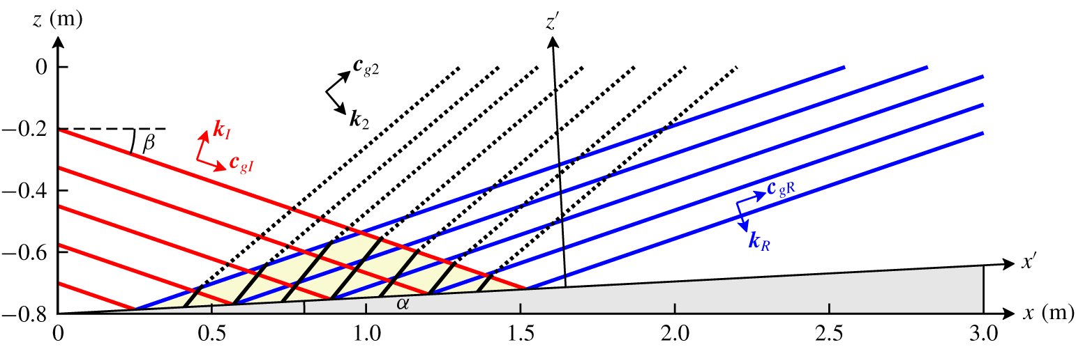
 $\unicode[STIX]{x1D6FD}>\unicode[STIX]{x1D6FC}$, the reflected wave propagates (away from and) against the slope and reflection is said to be sub-critical (see figure 1); for
 $\unicode[STIX]{x1D6FD}<\unicode[STIX]{x1D6FC}$, the reflected wave propagates along the slope and the reflection is super-critical. For
 $\unicode[STIX]{x1D6FD}$ close to
 $\unicode[STIX]{x1D6FC}$, referred to as critical incidence, focusing leads to strongly nonlinear processes close to the boundary (cf. McPhee-Shaw & Kunze Reference McPhee-Shaw and Kunze2002; Chalamalla et al. Reference Chalamalla, Vamsi, Gayen, Scotti and Sarkar2013) and organized vortex structures sometimes called bores are then observed (cf. Hosegood & van Haren Reference Hosegood and van Haren2004).
Sketch of the interaction between the incident and reflected waves in the  $(x,z)$ plane. The coordinates
 $(x^{\prime },z^{\prime })$ refer to the rotated frame of reference such that
 $x^{\prime }$ lies along the slope. The incident wave propagates in a vertical plane and has a finite width in the direction normal to propagation. This finite width contains four wavelengths in the sketch. The wave vector and group velocity of the incident wave are denoted
 $\boldsymbol{k}_{I}=(k,n_{I}k)$ and
 $\boldsymbol{c}_{gI}$; those for the reflected wave are
 $\boldsymbol{k}_{R}=(k,n_{R}k)$ and
 $\boldsymbol{c}_{gR}$, the components of
 $\boldsymbol{k}_{I}$ and
 $\boldsymbol{k}_{R}$ being expressed in the rotated reference frame. The red and blue solid lines represent phase lines of the incident and the reflected waves, respectively, and the interaction area between these waves is highlighted by a yellow triangle. The black solid lines in the interaction area represent phase lines of the second-harmonic ‘forced wave’
 $(2k,(n_{I}+n_{R})k,2\unicode[STIX]{x1D714})$ and black dashed lines correspond to the second-harmonic ‘free wave’
 $(2k,m_{2}\,k,2\unicode[STIX]{x1D714})$ able to propagate outside the interaction area (at resonance the black solid and dashed lines coincide, namely the forced wave becomes a free wave). The slope angle is
 $\unicode[STIX]{x1D6FC}$ and
 $\unicode[STIX]{x1D6FD}$ is the angle of incidence. The domain dimensions, expressed in metres, are those used in the numerical simulations.

Away from critical incidence, the interaction between the incident and the reflected waves leads to the generation of higher-harmonic motions of frequencies  $n\unicode[STIX]{x1D714}$ such that
 $2\leqslant n<\unicode[STIX]{x1D714}/N$ and amplitude
 $A^{n}$, where
 $A$ is the incident wave amplitude, with a much weaker impact on the fluid. However, as Thorpe (Reference Thorpe1987) (hereafter referred to as TH87) showed theoretically, the incident and the reflected plane waves can form a resonant triad with a second-harmonic wave resulting from their interaction, opening the possibility of breaking and mixing away from the slope. This result is valid only when the slope is inclined (
 $\unicode[STIX]{x1D6FC}\neq 0$) as no harmonic motion is produced when the incident plane wave reflects on a flat surface (Thorpe Reference Thorpe1968). In Thorpe (Reference Thorpe1997), the computation of the resonance condition is extended to a rotating fluid.
However, in natural flows, internal gravity waves do not propagate as pure plane waves. This is the case for the internal tide, which propagates as beams from a submarine mountain or a continental shelf. (The internal tide is the internal wave field resulting from the interaction of the barotropic tide with submarine topography.) This is also the case, to some extent, for lee waves, which propagate in the lee of a mountain and, most often, above it. In laboratory experiments as well, the generation of internal gravity waves always leads to wave packets of finite widths. Even the wave generator originally designed by Gostiaux et al. (Reference Gostiaux, Didelle, Mercier and Dauxois2007) to model pure plane waves produces a wave packet containing a finite number of wavelengths in the vertical plane, in the direction normal to the propagation of the packet. For a large number of wavelengths, say four and above, and a transverse width of the generator much larger than the wavelength, the incident wave structure may be assumed to be close to that of a pure plane wave, at least away from the boundaries of the packet; when the packet contains one wavelength, the wave structure is closer to that of a plane-wave beam. The wave packet produced by this wave generator will be referred to as a finite-width plane wave hereafter.
When a plane-wave beam incident on a surface interacts with the reflected beam, harmonic motions are produced, whether the surface is flat or not (Tabaei, Akylas & Lamb Reference Tabaei, Akylas and Lamb2005). A single beam is indeed a solution of the inviscid Boussinesq equations (Tabaei & Akylas Reference Tabaei and Akylas2003) while the superposition of two beams is not. This accounts for harmonics to be generated close to the boundary, where the beams interact, and this result holds for finite-width plane waves. The generation of higher harmonics by plane-wave beams (or by finite-width plane waves) reflecting either on a flat surface or on an inclined boundary has been addressed in several numerical and experimental works performed in a two-dimensional (or quasi-two-dimensional) vertical geometry. Gostiaux et al. (Reference Gostiaux, Dauxois, Didelle, Sommeria and Viboux2006) studied from laboratory experiments the structure of the higher harmonics resulting from the reflection of a finite-width plane wave on a flat surface. In Pairaud et al. (Reference Pairaud, Staquet, Sommeria and Mahdizadeh2010), the structure and evolution of an internal tide beam emitted from a two-dimensional topography is analysed from laboratory experiments and numerical simulations. It is shown that the reflection of the wave beam on the flat boundary at the foot of the slope leads to the generation of harmonic beams, consisting of free and trapped waves. Rodenborn et al. (Reference Rodenborn, Kiefer, Zhang and Swinney2011) considered a beam reflecting on a simple slope and investigated empirically the conditions that lead to the largest amplitude of the second-harmonic wave.
The purpose of the present paper is to examine the validity of the theory by TH87 when the conditions of a resonant triad involving an incident and a reflected wave of finite width and their second-harmonic wave are satisfied. In the first part, we revisit TH87 theory for the case of a pure plane wave reflecting on a uniform slope. It is indeed unclear whether this theory predicts a finite amplitude of the second-harmonic wave at resonance because the expression for this amplitude involves an indeterminacy (the numerator and denominator both vanish), which leads to the common inference in the literature that this amplitude diverges at resonance. In the second part, predictions of the theory of TH87 are determined for the case of an incident plane wave of finite width. The theoretical predictions are compared to the results of numerical simulations in a vertical plane, consistent with the resonant triad geometry, for parameters of laboratory experiments.
The plan of the paper is as follows. In § 2, the inviscid theory of TH87 for a pure plane wave incident on a uniform slope is presented and extended; we show that, at resonance, the amplitude of the second-harmonic plane wave actually grows linearly with distance from the slope. The predictions of the theory when the incident plane wave is of finite width are presented in § 3. We performed numerical simulations to estimate the validity of these predictions and the results are discussed in § 4. In § 5, the theoretical model is used again, in which viscous effects are introduced in order to compare the power transferred to the second-harmonic wave from the incident and reflected waves with the dissipated power of the latter waves. A summary and conclusions are given in § 6.
2 Nonlinear reflection of a pure plane wave
2.1 Governing equations
The governing equations are the Navier–Stokes equations in the Boussinesq approximation for a rotating fluid with uniform stratification,
 $$\begin{eqnarray}\displaystyle & \displaystyle \frac{\unicode[STIX]{x2202}^{}}{\unicode[STIX]{x2202}t^{}}\boldsymbol{u}+(\boldsymbol{u}\boldsymbol{\cdot }\unicode[STIX]{x1D735})\boldsymbol{u}=-\frac{1}{\unicode[STIX]{x1D70C}_{0}}\unicode[STIX]{x1D735}p-f\boldsymbol{e}_{z}\times \boldsymbol{u}+b\,\boldsymbol{e}_{z}, & \displaystyle\end{eqnarray}$$
 $$\begin{eqnarray}\displaystyle & \displaystyle \frac{\unicode[STIX]{x2202}^{}}{\unicode[STIX]{x2202}t^{}}b+\boldsymbol{u}\boldsymbol{\cdot }\unicode[STIX]{x1D735}b+N^{2}w=0, & \displaystyle\end{eqnarray}$$
 $$\begin{eqnarray}\displaystyle & \displaystyle \unicode[STIX]{x1D735}\boldsymbol{\cdot }\boldsymbol{u}=0, & \displaystyle\end{eqnarray}$$
 $$\begin{eqnarray}\displaystyle & \displaystyle \left.\boldsymbol{u}\boldsymbol{\cdot }\boldsymbol{n}\right|_{slope}=0. & \displaystyle\end{eqnarray}$$
 $\boldsymbol{u}=(u,v,w)$ is the velocity vector,
 $w$ being the vertical velocity component,
 $p$ is the non-hydrostatic pressure and
 $b$ is the buoyancy;
 $\unicode[STIX]{x1D70C}_{0}$ is a reference density and
 $\boldsymbol{e}_{z}$ and
 $\boldsymbol{n}$ are unit vectors along the vertical axis pointing upward and normal to the slope, respectively. The parameters
 $f$ and
 $N$ were defined in the Introduction. The last equation expresses the impermeability condition at the boundary.
We shall assume that wave propagation occurs in the vertical  $(x,z)$ plane and that the problem is invariant in the
 $y$-direction. Therefore all three velocity components depend on
 $x$ and
 $z$ (and on time) only and the incompressibility condition (2.1c) reduces to
 $\unicode[STIX]{x2202}u/\unicode[STIX]{x2202}x+\unicode[STIX]{x2202}w/\unicode[STIX]{x2202}z=0$. As usual, this condition is automatically satisfied if a streamfunction
 $\unicode[STIX]{x1D713}$ is introduced. Expressing the velocity vector as
 $\boldsymbol{u}=(\unicode[STIX]{x2202}\unicode[STIX]{x1D713}/\unicode[STIX]{x2202}z,v,-\unicode[STIX]{x2202}\unicode[STIX]{x1D713}/\unicode[STIX]{x2202}x)$ and combining the equations for
 $u$ and
 $w$ into a single equation for the vorticity
 $\unicode[STIX]{x2202}w/\unicode[STIX]{x2202}x-\unicode[STIX]{x2202}u/\unicode[STIX]{x2202}z=-\unicode[STIX]{x1D6FB}^{2}\unicode[STIX]{x1D713}$, equations (2.1) become
 $$\begin{eqnarray}\displaystyle & \displaystyle \frac{\unicode[STIX]{x2202}^{}}{\unicode[STIX]{x2202}t^{}}\unicode[STIX]{x1D6FB}^{2}\unicode[STIX]{x1D713}+\frac{\unicode[STIX]{x2202}^{}}{\unicode[STIX]{x2202}x^{}}b-f\frac{\unicode[STIX]{x2202}^{}}{\unicode[STIX]{x2202}z^{}}v=J(\unicode[STIX]{x1D713},\unicode[STIX]{x1D6FB}^{2}\unicode[STIX]{x1D713}), & \displaystyle\end{eqnarray}$$
 $$\begin{eqnarray}\displaystyle & \displaystyle \frac{\unicode[STIX]{x2202}^{}}{\unicode[STIX]{x2202}t^{}}v+f\frac{\unicode[STIX]{x2202}^{}}{\unicode[STIX]{x2202}z^{}}\unicode[STIX]{x1D713}=J(\unicode[STIX]{x1D713},v), & \displaystyle\end{eqnarray}$$
 $$\begin{eqnarray}\displaystyle & \displaystyle \frac{\unicode[STIX]{x2202}^{}}{\unicode[STIX]{x2202}t^{}}b-N^{2}\frac{\unicode[STIX]{x2202}^{}}{\unicode[STIX]{x2202}x^{}}\unicode[STIX]{x1D713}=J(\unicode[STIX]{x1D713},b), & \displaystyle\end{eqnarray}$$
 $$\begin{eqnarray}\displaystyle & \displaystyle \left.\boldsymbol{u}\boldsymbol{\cdot }\boldsymbol{n}\right|_{slope}=0, & \displaystyle\end{eqnarray}$$
 $J$ designates the Jacobian operator. Equation (2.2a) is rewritten by taking the time derivative and by replacing the fields
 $\unicode[STIX]{x2202}v/\unicode[STIX]{x2202}t$ and
 $\unicode[STIX]{x2202}b/\unicode[STIX]{x2202}t$ by their expressions from equations (2.2b) and (2.2c), respectively. This yields
 $$\begin{eqnarray}\frac{\unicode[STIX]{x2202}^{2}}{\unicode[STIX]{x2202}t^{2}}\unicode[STIX]{x1D6FB}^{2}\unicode[STIX]{x1D713}+N^{2}\frac{\unicode[STIX]{x2202}^{2}}{\unicode[STIX]{x2202}x^{2}}\unicode[STIX]{x1D713}+f^{2}\frac{\unicode[STIX]{x2202}^{2}}{\unicode[STIX]{x2202}z^{2}}\unicode[STIX]{x1D713}=\frac{\unicode[STIX]{x2202}^{}}{\unicode[STIX]{x2202}t^{}}J(\unicode[STIX]{x1D713},\unicode[STIX]{x1D6FB}^{2}\unicode[STIX]{x1D713})-\frac{\unicode[STIX]{x2202}^{}}{\unicode[STIX]{x2202}x^{}}J(\unicode[STIX]{x1D713},b)+f\frac{\unicode[STIX]{x2202}^{}}{\unicode[STIX]{x2202}z^{}}J(\unicode[STIX]{x1D713},v).\end{eqnarray}$$
The set of equations (2.2b), (2.2c), (2.2d) and (2.3) will be referred to as equations ( ${\mathcal{E}}$) hereafter.
Let us rewrite this set of equations in a rotated coordinate system ( $x^{\prime },z^{\prime }$) with
 $x^{\prime }$ and
 $z^{\prime }$ being the along- and normal-slope coordinates respectively. Following TH87, we use the convenient abbreviations
 $c_{\unicode[STIX]{x1D6FC}}$,
 $s_{\unicode[STIX]{x1D6FC}}$,
 $c_{\unicode[STIX]{x1D6FD}}$ and
 $s_{\unicode[STIX]{x1D6FD}}$, standing for
 $\cos \unicode[STIX]{x1D6FC}$,
 $\sin \unicode[STIX]{x1D6FC}$,
 $\cos \unicode[STIX]{x1D6FD}$ and
 $\sin \unicode[STIX]{x1D6FD}$, respectively. Thus
 $(x^{\prime },z^{\prime })=(xc_{\unicode[STIX]{x1D6FC}}+zs_{\unicode[STIX]{x1D6FC}},zc_{\unicode[STIX]{x1D6FC}}-xs_{\unicode[STIX]{x1D6FC}})$,
 $\unicode[STIX]{x1D6FC}$ being the slope angle. In this coordinate system, for a pure plane wave with frequency
 $\unicode[STIX]{x1D714}$ and along- and normal-slope wavenumbers
 $k$ and
 $nk$, respectively, the dispersion relation (1.1) becomes
 $$\begin{eqnarray}\unicode[STIX]{x1D714}^{2}=N^{2}s_{\unicode[STIX]{x1D6FD}}^{2}+f^{2}c_{\unicode[STIX]{x1D6FD}}^{2}=N^{2}\frac{\left(ns_{\unicode[STIX]{x1D6FC}}-c_{\unicode[STIX]{x1D6FC}}\right)^{2}}{1+n^{2}}+f^{2}\frac{\left(s_{\unicode[STIX]{x1D6FC}}+nc_{\unicode[STIX]{x1D6FC}}\right)^{2}}{1+n^{2}}.\end{eqnarray}$$
Solving this equation for  $n$ yields two roots
 $$\begin{eqnarray}\quad n_{I}=\frac{s_{\unicode[STIX]{x1D6FD}}c_{\unicode[STIX]{x1D6FD}}-s_{\unicode[STIX]{x1D6FC}}c_{\unicode[STIX]{x1D6FC}}}{s_{\unicode[STIX]{x1D6FD}}^{2}-s_{\unicode[STIX]{x1D6FC}}^{2}},\quad \text{and}\quad n_{R}=-\frac{s_{\unicode[STIX]{x1D6FD}}c_{\unicode[STIX]{x1D6FD}}+s_{\unicode[STIX]{x1D6FC}}c_{\unicode[STIX]{x1D6FC}}}{s_{\unicode[STIX]{x1D6FD}}^{2}-s_{\unicode[STIX]{x1D6FC}}^{2}},\end{eqnarray}$$
which are associated with the incident and reflected wave, respectively. Note that these roots are no longer defined as in TH87 as we have chosen to scale the normal-slope wavenumber by the along-slope wavenumber  $k$. This turns out to be more convenient for some further calculations as
 $k$ is conserved through the reflection process.
Equations ( ${\mathcal{E}}$) are made non-dimensional using the horizontal velocity amplitude of the incident wave, denoted
 $U$, as a velocity scale, its wavelength
 $\unicode[STIX]{x1D706}$ as a length scale and
 $1/N$ as a time scale. These scales come into play in the non-dimensional equations of motions through a Froude number
 $Fr=U/\unicode[STIX]{x1D706}N$ and through the parameter
 $f/N$. The Froude number can be interpreted as a non-dimensional amplitude of the incident wave field. When rotation effects can be ignored, this Froude number can be rewritten as
 $Fr=s/2\unicode[STIX]{x03C0}$, where
 $s=U/c_{x}$ is the wave steepness (
 $c_{x}$ is the phase velocity in the
 $x$-direction).
When expressed in the rotated coordinate system and made non-dimensional, equations ( ${\mathcal{E}}$) become, keeping the same notations for the non-dimensional variables as well as for the non-dimensional parameters
 $N$ and
 $f$ to keep track of the Brunt–Väisälä frequency (otherwise equal to
 $1$) in the equations,
 $$\begin{eqnarray}\displaystyle & & \displaystyle \frac{\unicode[STIX]{x2202}^{2}}{\unicode[STIX]{x2202}t^{2}}\unicode[STIX]{x1D6FB}^{2}\unicode[STIX]{x1D713}+N^{2}\left(c_{\unicode[STIX]{x1D6FC}}\frac{\unicode[STIX]{x2202}^{}}{\unicode[STIX]{x2202}{x^{\prime }}^{}}-s_{\unicode[STIX]{x1D6FC}}\frac{\unicode[STIX]{x2202}^{}}{\unicode[STIX]{x2202}{z^{\prime }}^{}}\right)^{2}\unicode[STIX]{x1D713}+f^{2}\left(s_{\unicode[STIX]{x1D6FC}}\frac{\unicode[STIX]{x2202}^{}}{\unicode[STIX]{x2202}{x^{\prime }}^{}}+c_{\unicode[STIX]{x1D6FC}}\frac{\unicode[STIX]{x2202}^{}}{\unicode[STIX]{x2202}{z^{\prime }}^{}}\right)^{2}\unicode[STIX]{x1D713}\nonumber\\ \displaystyle & & \displaystyle \qquad =Fr\left[\frac{\unicode[STIX]{x2202}^{}}{\unicode[STIX]{x2202}t^{}}J(\unicode[STIX]{x1D713},\unicode[STIX]{x1D6FB}^{2}\unicode[STIX]{x1D713})-\left(c_{\unicode[STIX]{x1D6FC}}\frac{\unicode[STIX]{x2202}^{}}{\unicode[STIX]{x2202}{x^{\prime }}^{}}-s_{\unicode[STIX]{x1D6FC}}\frac{\unicode[STIX]{x2202}^{}}{\unicode[STIX]{x2202}{z^{\prime }}^{}}\right)J(\unicode[STIX]{x1D713},b)\right.\nonumber\\ \displaystyle & & \displaystyle \qquad \quad \left.+\,f\left(s_{\unicode[STIX]{x1D6FC}}\frac{\unicode[STIX]{x2202}^{}}{\unicode[STIX]{x2202}{x^{\prime }}^{}}+c_{\unicode[STIX]{x1D6FC}}\frac{\unicode[STIX]{x2202}^{}}{\unicode[STIX]{x2202}{z^{\prime }}^{}}\right)J(\unicode[STIX]{x1D713},v)\right],\end{eqnarray}$$
 $$\begin{eqnarray}\displaystyle & \displaystyle \frac{\unicode[STIX]{x2202}^{}}{\unicode[STIX]{x2202}t^{}}v+f\left(s_{\unicode[STIX]{x1D6FC}}\frac{\unicode[STIX]{x2202}^{}}{\unicode[STIX]{x2202}{x^{\prime }}^{}}+c_{\unicode[STIX]{x1D6FC}}\frac{\unicode[STIX]{x2202}^{}}{\unicode[STIX]{x2202}{z^{\prime }}^{}}\right)\unicode[STIX]{x1D713}=Fr\,J(\unicode[STIX]{x1D713},v), & \displaystyle\end{eqnarray}$$
 $$\begin{eqnarray}\displaystyle & \displaystyle \frac{\unicode[STIX]{x2202}^{}}{\unicode[STIX]{x2202}t^{}}b-N^{2}\left(c_{\unicode[STIX]{x1D6FC}}\frac{\unicode[STIX]{x2202}^{}}{\unicode[STIX]{x2202}{x^{\prime }}^{}}-s_{\unicode[STIX]{x1D6FC}}\frac{\unicode[STIX]{x2202}^{}}{\unicode[STIX]{x2202}{z^{\prime }}^{}}\right)\unicode[STIX]{x1D713}=Fr\,J(\unicode[STIX]{x1D713},b), & \displaystyle\end{eqnarray}$$
 $$\begin{eqnarray}\displaystyle & \displaystyle \left.\frac{\unicode[STIX]{x2202}^{}\unicode[STIX]{x1D713}}{\unicode[STIX]{x2202}{x^{\prime }}^{}}\right|_{z^{\prime }=0}=0. & \displaystyle\end{eqnarray}$$
In the following,  $Fr$ is considered as a small parameter (i.e.
 $Fr\ll 1$), namely the wave dynamics is weakly nonlinear. The
 $\unicode[STIX]{x1D713}$,
 $b$ and
 $v$ fields can thus be decomposed into a multiple scale expansion as
 $\unicode[STIX]{x1D713}=\unicode[STIX]{x1D713}_{1}+Fr\,\unicode[STIX]{x1D713}_{2}+o(Fr^{2})$,
 $b=b_{1}+Fr\,b_{2}+o(Fr^{2})$ and
 $v=v_{1}+Fr\,v_{2}+o(Fr^{2})$. Introducing these expansions in the equations of motion (2.6), the resulting equations can be solved order by order, by matching terms multiplied by the same power of
 $Fr$. At each order the solution satisfies the same linear operator with a right-hand side determined by lower-order nonlinear terms. Identifying terms multiplied by
 $Fr^{0}$, the first-order fields
 $\unicode[STIX]{x1D713}_{1}$,
 $v_{1}$ and
 $b_{1}$ are thus found to satisfy the homogeneous linear wave equations. Matching terms multiplied by
 $Fr^{1}$ shows that the second-order fields
 $\unicode[STIX]{x1D713}_{2}$,
 $v_{2}$ and
 $b_{2}$ are solutions of the same linear operator forced by nonlinear terms solely involving the first-order fields. The detailed calculations associated with this general principle are now presented.
2.2 First-order solution
The linear equation satisfied by  $\unicode[STIX]{x1D713}_{1}$ is given by
 $$\begin{eqnarray}\frac{\unicode[STIX]{x2202}^{2}}{\unicode[STIX]{x2202}t^{2}}\unicode[STIX]{x1D6FB}^{2}\unicode[STIX]{x1D713}_{1}+N^{2}\left(c_{\unicode[STIX]{x1D6FC}}\frac{\unicode[STIX]{x2202}^{}}{\unicode[STIX]{x2202}{x^{\prime }}^{}}-s_{\unicode[STIX]{x1D6FC}}\frac{\unicode[STIX]{x2202}^{}}{\unicode[STIX]{x2202}{z^{\prime }}^{}}\right)^{2}\unicode[STIX]{x1D713}_{1}+f^{2}\left(s_{\unicode[STIX]{x1D6FC}}\frac{\unicode[STIX]{x2202}^{}}{\unicode[STIX]{x2202}{x^{\prime }}^{}}+c_{\unicode[STIX]{x1D6FC}}\frac{\unicode[STIX]{x2202}^{}}{\unicode[STIX]{x2202}{z^{\prime }}^{}}\right)^{2}\unicode[STIX]{x1D713}_{1}=0\end{eqnarray}$$
with the boundary condition
 $$\begin{eqnarray}\left.\frac{\unicode[STIX]{x2202}^{}\unicode[STIX]{x1D713}_{1}}{\unicode[STIX]{x2202}{x^{\prime }}^{}}\right|_{z^{\prime }=0}=0.\end{eqnarray}$$
Looking for a pure plane-wave solution with wavenumbers  $(k,nk)$ and frequency
 $\unicode[STIX]{x1D714}$, the wave parameters are found to satisfy the dispersion relation (2.4), implying that the solution
 $\unicode[STIX]{x1D713}_{1}$ is a linear superposition of waves with wavenumbers
 $(k,n_{R}k)$ and
 $(k,n_{I}k)$, with
 $n_{I}$ and
 $n_{R}$ given by (2.5). Imposing the boundary condition (2.7b) yields (Phillips Reference Phillips1966):
 $$\begin{eqnarray}\unicode[STIX]{x1D713}_{1}=a_{1}\left[\sin \left(kx^{\prime }+n_{I}kz^{\prime }-\unicode[STIX]{x1D714}t\right)-\sin \left(kx^{\prime }+n_{R}kz^{\prime }-\unicode[STIX]{x1D714}t\right)\right].\end{eqnarray}$$
The first-order streamfunction is therefore the sum of a wave incident on the slope, which we denote for simplicity as  $(k,n_{I}k,\unicode[STIX]{x1D714})$, and of its reflected counterpart
 $(k,n_{R}k,\unicode[STIX]{x1D714})$. The wave amplitude
 $a_{1}$ is arbitrary. The streamfunction
 $\unicode[STIX]{x1D713}_{1}$ is also defined up to a constant additional phase, chosen to be
 $0$ in the present case, which does not imply any loss of generality.
Once  $\unicode[STIX]{x1D713}_{1}$ is known,
 $v_{1}$ and
 $b_{1}$ are inferred from the equations
 $$\begin{eqnarray}\frac{\unicode[STIX]{x2202}^{}}{\unicode[STIX]{x2202}t^{}}v_{1}+f\left(s_{\unicode[STIX]{x1D6FC}}\frac{\unicode[STIX]{x2202}^{}}{\unicode[STIX]{x2202}{x^{\prime }}^{}}+c_{\unicode[STIX]{x1D6FC}}\frac{\unicode[STIX]{x2202}^{}}{\unicode[STIX]{x2202}{z^{\prime }}^{}}\right)\unicode[STIX]{x1D713}_{1}=0\end{eqnarray}$$
and
 $$\begin{eqnarray}\frac{\unicode[STIX]{x2202}^{}}{\unicode[STIX]{x2202}t^{}}b_{1}-N^{2}\left(c_{\unicode[STIX]{x1D6FC}}\frac{\unicode[STIX]{x2202}^{}}{\unicode[STIX]{x2202}{x^{\prime }}^{}}-s_{\unicode[STIX]{x1D6FC}}\frac{\unicode[STIX]{x2202}^{}}{\unicode[STIX]{x2202}{z^{\prime }}^{}}\right)\unicode[STIX]{x1D713}_{1}=0,\end{eqnarray}$$
which yields
 $$\begin{eqnarray}v_{1}=\frac{a_{1}fk}{\unicode[STIX]{x1D714}}\left[(s_{\unicode[STIX]{x1D6FC}}+c_{\unicode[STIX]{x1D6FC}}n_{I})\sin \left(kx^{\prime }+n_{I}kz^{\prime }-\unicode[STIX]{x1D714}t\right)-(s_{\unicode[STIX]{x1D6FC}}+c_{\unicode[STIX]{x1D6FC}}n_{R})\sin \left(kx^{\prime }+n_{R}kz^{\prime }-\unicode[STIX]{x1D714}t\right)\right]\end{eqnarray}$$
and
 $$\begin{eqnarray}b_{1}=\frac{a_{1}N^{2}k}{\unicode[STIX]{x1D714}}\left[(c_{\unicode[STIX]{x1D6FC}}-s_{\unicode[STIX]{x1D6FC}}n_{R})\sin \left(kx^{\prime }+n_{R}kz^{\prime }-\unicode[STIX]{x1D714}t\right)-(c_{\unicode[STIX]{x1D6FC}}-s_{\unicode[STIX]{x1D6FC}}n_{I})\sin \left(kx^{\prime }+n_{I}kz^{\prime }-\unicode[STIX]{x1D714}t\right)\right].\end{eqnarray}$$
2.3 Second-order solution
Matching terms proportional to  $Fr$ in (2.6) gives the equations for the second-order component. The equation for
 $\unicode[STIX]{x1D713}_{2}$ is
 $$\begin{eqnarray}\displaystyle & & \displaystyle \frac{\unicode[STIX]{x2202}^{2}}{\unicode[STIX]{x2202}t^{2}}\unicode[STIX]{x1D6FB}^{2}\unicode[STIX]{x1D713}_{2}+N^{2}\left(c_{\unicode[STIX]{x1D6FC}}\frac{\unicode[STIX]{x2202}^{}}{\unicode[STIX]{x2202}{x^{\prime }}^{}}-s_{\unicode[STIX]{x1D6FC}}\frac{\unicode[STIX]{x2202}^{}}{\unicode[STIX]{x2202}{z^{\prime }}^{}}\right)^{2}\unicode[STIX]{x1D713}_{2}+f^{2}\left(s_{\unicode[STIX]{x1D6FC}}\frac{\unicode[STIX]{x2202}^{}}{\unicode[STIX]{x2202}{x^{\prime }}^{}}+c_{\unicode[STIX]{x1D6FC}}\frac{\unicode[STIX]{x2202}^{}}{\unicode[STIX]{x2202}{z^{\prime }}^{}}\right)^{2}\unicode[STIX]{x1D713}_{2}\nonumber\\ \displaystyle & & \displaystyle \qquad =\frac{\unicode[STIX]{x2202}^{}}{\unicode[STIX]{x2202}t^{}}J(\unicode[STIX]{x1D713}_{1},\unicode[STIX]{x1D6FB}^{2}\unicode[STIX]{x1D713}_{1})-\left(c_{\unicode[STIX]{x1D6FC}}\frac{\unicode[STIX]{x2202}^{}}{\unicode[STIX]{x2202}{x^{\prime }}^{}}-s_{\unicode[STIX]{x1D6FC}}\frac{\unicode[STIX]{x2202}^{}}{\unicode[STIX]{x2202}{z^{\prime }}^{}}\right)J(\unicode[STIX]{x1D713}_{1},b_{1})\nonumber\\ \displaystyle & & \displaystyle \qquad \quad +\,f\left(s_{\unicode[STIX]{x1D6FC}}\frac{\unicode[STIX]{x2202}^{}}{\unicode[STIX]{x2202}{x^{\prime }}^{}}+c_{\unicode[STIX]{x1D6FC}}\frac{\unicode[STIX]{x2202}^{}}{\unicode[STIX]{x2202}{z^{\prime }}^{}}\right)J(\unicode[STIX]{x1D713}_{1},v_{1})\end{eqnarray}$$
with the boundary condition
 $$\begin{eqnarray}\left.\frac{\unicode[STIX]{x2202}^{}\unicode[STIX]{x1D713}_{2}}{\unicode[STIX]{x2202}{x^{\prime }}^{}}\right|_{z^{\prime }=0}=0.\end{eqnarray}$$
The solution of equations (2.13), which generalizes TH87 solution to a rotating fluid, is,
 $$\begin{eqnarray}\displaystyle \unicode[STIX]{x1D713}_{2} & = & \displaystyle 3a_{1}^{2}k^{2}\unicode[STIX]{x1D714}\frac{s_{\unicode[STIX]{x1D6FD}}^{2}c_{\unicode[STIX]{x1D6FD}}^{2}s_{\unicode[STIX]{x1D6FC}}c_{\unicode[STIX]{x1D6FC}}}{(s_{\unicode[STIX]{x1D6FD}}^{2}-s_{\unicode[STIX]{x1D6FC}}^{2})D}[\sin (2kx^{\prime }+m_{2}kz^{\prime }-2\unicode[STIX]{x1D714}t)-\sin (2kx^{\prime }+(n_{I}+n_{R})kz^{\prime }-2\unicode[STIX]{x1D714}t)]\nonumber\\ \displaystyle & & \displaystyle -\,\frac{a_{1}^{2}k^{2}}{\unicode[STIX]{x1D714}}\frac{s_{\unicode[STIX]{x1D6FD}}c_{\unicode[STIX]{x1D6FD}}}{s_{\unicode[STIX]{x1D6FD}}^{2}-s_{\unicode[STIX]{x1D6FC}}^{2}}\sin ((n_{I}-n_{R})kz^{\prime })\end{eqnarray}$$
with
 $$\begin{eqnarray}D=N^{2}s_{\unicode[STIX]{x1D6FD}}^{2}\left(4s_{\unicode[STIX]{x1D6FD}}^{4}-7s_{\unicode[STIX]{x1D6FD}}^{2}s_{\unicode[STIX]{x1D6FC}}^{2}+4s_{\unicode[STIX]{x1D6FC}}^{2}-s_{\unicode[STIX]{x1D6FD}}^{2}\right)+f^{2}c_{\unicode[STIX]{x1D6FD}}^{2}\left(4s_{\unicode[STIX]{x1D6FD}}^{4}-7s_{\unicode[STIX]{x1D6FD}}^{2}s_{\unicode[STIX]{x1D6FC}}^{2}+3s_{\unicode[STIX]{x1D6FC}}^{2}\right)\end{eqnarray}$$
and
 $$\begin{eqnarray}m_{2}=\frac{-2s_{\unicode[STIX]{x1D6FC}}c_{\unicode[STIX]{x1D6FC}}(N^{2}-f^{2})+2\sqrt{4s_{\unicode[STIX]{x1D6FD}}^{2}N^{4}(1-4s_{\unicode[STIX]{x1D6FD}}^{2})+4c_{\unicode[STIX]{x1D6FD}}^{2}f^{4}(1-4c_{\unicode[STIX]{x1D6FD}}^{2})+N^{2}f^{2}(3-32s_{\unicode[STIX]{x1D6FD}}^{2}c_{\unicode[STIX]{x1D6FD}}^{2})}}{N^{2}(4s_{\unicode[STIX]{x1D6FD}}^{2}-s_{\unicode[STIX]{x1D6FC}}^{2})+f^{2}(4c_{\unicode[STIX]{x1D6FD}}^{2}-c_{\unicode[STIX]{x1D6FC}}^{2})}.\end{eqnarray}$$
Details of this calculation can be found in § A.1 where the full second-order solution is derived.
The second-order streamfunction (2.14) is the sum of an oscillatory component (for  $\unicode[STIX]{x1D6FC}\neq 0$) and a steady component. The oscillatory component, referred to as the second-harmonic wave in the Introduction, is made of two terms, associated with the waves
 $(2k,m_{2}k,2\unicode[STIX]{x1D714})$ and
 $(2k,(n_{I}+n_{R})k,2\unicode[STIX]{x1D714})$. The former term is the solution of the homogeneous equation associated with (2.13a) so that the wave
 $(2k,m_{2}k,2\unicode[STIX]{x1D714})$ satisfies the dispersion relation and radiates energy away from the boundary. This term is called a ‘free wave’ by TH87. As detailed in § A.1, equation (2.14) is obtained by adding to this homogeneous solution a particular solution of the complete equation, referred to as a ‘forced’ wave by TH87, and by prescribing the homogeneous solution parameters through the boundary condition (2.13b). The forced wave becomes a free wave when
 $(2k,(n_{I}+n_{R})k,2\unicode[STIX]{x1D714})$ satisfies the dispersion relation, namely when
 $n_{I}+n_{R}=m_{2}$; in this case, the incident, reflected and second-harmonic waves form a resonant triad. A sketch of the interaction between the incident and reflected waves for conditions away from resonance is displayed in figure 1.
The steady component of (2.14) is an Eulerian mean current opposing the Stokes drift associated with the first-order solution ((2.8), (2.11), (2.12)), as stated by TH87 and Thorpe (Reference Thorpe1997). Hence, the total Lagrangian mean flow, which is the sum of the Eulerian mean flow and of the Stokes drift (Longuet-Higgins Reference Longuet-Higgins1969), is zero (see § A.3). Indeed, because of the sloping boundary, there cannot be any horizontal mass transport in the present two-dimensional configuration, implying that the Lagrangian mean flow must vanish.
We now consider the oscillatory component, denoted  $\unicode[STIX]{x1D713}_{2}^{h}$. The denominator of its amplitude goes to
 $0$ for values of
 $(\unicode[STIX]{x1D6FC},\unicode[STIX]{x1D6FD})$ satisfying
 $D=0$. For
 $f=0$, these values span the intervals
 $[0,8.21^{\circ }]$ for
 $\unicode[STIX]{x1D6FC}$ and
 $[0,30^{\circ }]$ for
 $\unicode[STIX]{x1D6FD}$, these ranges shrinking to empty intervals as
 $f/N$ increases and reaches
 $0.5$. As stated in TH87 and detailed in § A.2, the condition
 $D=0$ corresponds to the case of a resonant triad between the incident and reflected waves and the second-harmonic free wave. Since
 $m_{2}=n_{I}+n_{R}$ in this case, as just discussed, the oscillatory component in (2.14) is an indeterminate form
 $0/0$ as
 $D\rightarrow 0$. One aim of the present paper is to remove this indeterminacy to clarify the behaviour of the oscillatory component at resonance. For this purpose, we rewrite the oscillatory component of
 $\unicode[STIX]{x1D713}_{2}$ as
 $$\begin{eqnarray}\unicode[STIX]{x1D713}_{2}^{h}=6a_{1}^{2}k^{2}\unicode[STIX]{x1D714}\,\frac{s_{\unicode[STIX]{x1D6FD}}^{2}c_{\unicode[STIX]{x1D6FD}}^{2}s_{\unicode[STIX]{x1D6FC}}c_{\unicode[STIX]{x1D6FC}}}{s_{\unicode[STIX]{x1D6FD}}^{2}-s_{\unicode[STIX]{x1D6FC}}^{2}}\frac{\sin (\unicode[STIX]{x1D6FF}kz^{\prime })}{D}\,\cos (2kx^{\prime }+(m_{2}-\unicode[STIX]{x1D6FF})kz^{\prime }-2\unicode[STIX]{x1D714}t),\end{eqnarray}$$
where  $\unicode[STIX]{x1D6FF}=\frac{1}{2}(m_{2}-(n_{I}+n_{R}))$. For
 $\unicode[STIX]{x1D6FC}\neq 0$, one can show that
 $$\begin{eqnarray}\unicode[STIX]{x1D6FF}\underset{D\rightarrow 0}{{\sim}}\frac{D}{6s_{\unicode[STIX]{x1D6FC}}c_{\unicode[STIX]{x1D6FC}}\left(s_{\unicode[STIX]{x1D6FD}}^{2}-s_{\unicode[STIX]{x1D6FC}}^{2}\right)\unicode[STIX]{x1D714}^{2}},\end{eqnarray}$$
so that
 $$\begin{eqnarray}\frac{\sin (\unicode[STIX]{x1D6FF}kz^{\prime })}{D}\underset{D\rightarrow 0}{\rightarrow }\frac{kz^{\prime }}{6s_{\unicode[STIX]{x1D6FC}}c_{\unicode[STIX]{x1D6FC}}\left(s_{\unicode[STIX]{x1D6FD}}^{2}-s_{\unicode[STIX]{x1D6FC}}^{2}\right)\unicode[STIX]{x1D714}^{2}}\end{eqnarray}$$
(see § A.2 for details). Hence, as  $D\rightarrow 0$, the second-harmonic wave becomes
 $$\begin{eqnarray}\unicode[STIX]{x1D713}_{2}^{h}=\frac{a_{1}^{2}k^{2}}{\unicode[STIX]{x1D714}}\frac{s_{\unicode[STIX]{x1D6FD}}^{2}c_{\unicode[STIX]{x1D6FD}}^{2}}{(s_{\unicode[STIX]{x1D6FD}}^{2}-s_{\unicode[STIX]{x1D6FC}}^{2})^{2}}\,kz^{\prime }\cos (2kx^{\prime }+(n_{I}+n_{R})kz^{\prime }-2\unicode[STIX]{x1D714}t).\end{eqnarray}$$
The amplitude of the second-harmonic wave is thus a periodic function of the distance from the slope  $z^{\prime }$ whose period
 $2\unicode[STIX]{x03C0}/\unicode[STIX]{x1D6FF}k$ goes to infinity as
 $(\unicode[STIX]{x1D6FC},\unicode[STIX]{x1D6FD})$ approaches the resonance condition
 $D=0$. At resonance, this amplitude grows linearly from the slope. The linear growth with distance from the slope is consistent with the response of a resonant forcing; it is well known for instance that the amplitude of a resonantly forced harmonic oscillator grows linearly with time. This linear growth being predicted by a weakly nonlinear theory, it is theoretically valid for a distance
 $z^{\prime }$ from the slope such that the second-harmonic wave amplitude remains small compared to the first-order wave amplitude, namely
 $Fr\,|\unicode[STIX]{x1D713}_{2}^{h}|\ll |\unicode[STIX]{x1D713}_{1}|$.
3 Nonlinear reflection of a plane wave of finite width
The results presented in § 2.3 have been obtained for a pure plane wave. As discussed in the Introduction, this type of wave is commonly modelled in laboratory experiments by a wave generator, which creates in practice a wave packet containing a finite number of wavelengths in the direction normal to the propagation of the packet. The interaction area between the incident and the reflected waves is now spatially bounded and is represented by the yellow triangle in figure 1. In the present section, we compute the amplitude of the second-harmonic wave amplitude when resonant conditions are met for this generation method. The incident wave field is modelled theoretically as a plane wave with a finite number of wavelengths in the direction normal to wave propagation, with no envelope. In § 4, we compare the theoretical predictions with numerical simulations for an incident wave with various widths.
We recall that, to be valid, the theory requires the amplitude of  $Fr\,\unicode[STIX]{x1D713}_{2}$ to stay small with respect to the amplitude of
 $\unicode[STIX]{x1D713}_{1}$. Since we focus on the oscillatory component of
 $\unicode[STIX]{x1D713}_{2}$, namely
 $\unicode[STIX]{x1D713}_{2}^{h}$, we scale the amplitude of
 $Fr\,\unicode[STIX]{x1D713}_{2}^{h}$ with that of
 $\unicode[STIX]{x1D713}_{1}$. More precisely, we scale
 $Fr\Vert \unicode[STIX]{x1D713}_{2}^{h}\Vert$ by
 $\Vert \unicode[STIX]{x1D713}_{1}\Vert$ where the norm
 $\Vert \cdot \Vert$ is the infinity norm in space and time. This norm is defined by
 $\Vert \unicode[STIX]{x1D713}\Vert =\max _{(\boldsymbol{x},t)\in \unicode[STIX]{x1D6FA}\times \mathbb{R}^{+}}|\unicode[STIX]{x1D713}|$, where
 $\unicode[STIX]{x1D6FA}$ is the interaction area between the incident and reflected waves. We thus compute the ratio
 $$\begin{eqnarray}R^{th}=\frac{Fr\Vert \unicode[STIX]{x1D713}_{2}^{h}\Vert }{\Vert \unicode[STIX]{x1D713}_{1}\Vert },\end{eqnarray}$$
the  $th$ superscript standing for theoretical. At resonance, the amplitude of
 $\unicode[STIX]{x1D713}_{2}^{h}$ should reach a maximum value at the largest distance from the slope in the interaction area, which coincides with the top of the yellow triangle. Our purpose here is (i) to compute
 $R^{th}$ as a function of the parameters of the incident wave and (ii) to investigate the conditions under which the theory is strictly valid (namely
 $R^{th}\ll 1$).
Let us compute  $\Vert \unicode[STIX]{x1D713}_{1}\Vert$ and
 $\Vert \unicode[STIX]{x1D713}_{2}^{h}\Vert$. If one rewrites
 $\unicode[STIX]{x1D713}_{1}$ in the same way as
 $\unicode[STIX]{x1D713}_{2}^{h}$, i.e.
 $$\begin{eqnarray}\unicode[STIX]{x1D713}_{1}=2a_{1}\sin \left(\frac{n_{I}-n_{R}}{2}kz^{\prime }\right)\cos \left(kx^{\prime }+\frac{n_{I}+n_{R}}{2}kz^{\prime }-\unicode[STIX]{x1D714}t\right),\end{eqnarray}$$
the expressions of  $\Vert \unicode[STIX]{x1D713}_{1}\Vert$ and
 $\Vert \unicode[STIX]{x1D713}_{2}^{h}\Vert$ are given by
 $$\begin{eqnarray}\Vert \unicode[STIX]{x1D713}_{1}\Vert =2a_{1}\max _{0\leqslant kz^{\prime }\leqslant kh}\left\{\sin \left(\frac{n_{I}-n_{R}}{2}kz^{\prime }\right)\right\}\end{eqnarray}$$
and
 $$\begin{eqnarray}\Vert \unicode[STIX]{x1D713}_{2}^{h}\Vert =6a_{1}^{2}k^{2}\unicode[STIX]{x1D714}\frac{s_{\unicode[STIX]{x1D6FD}}^{2}c_{\unicode[STIX]{x1D6FD}}^{2}s_{\unicode[STIX]{x1D6FC}}c_{\unicode[STIX]{x1D6FC}}}{s_{\unicode[STIX]{x1D6FD}}^{2}-s_{\unicode[STIX]{x1D6FC}}^{2}}\max _{0\leqslant kz^{\prime }\leqslant kh}\left\{\frac{\sin (\unicode[STIX]{x1D6FF}kz^{\prime })}{D}\right\},\end{eqnarray}$$
where  $h$ is the height of the interaction triangle normal to the slope. Introducing
 $n_{\unicode[STIX]{x1D706}}$, the number of wavelengths contained in the incident wave, and thanks to simple trigonometric calculations, one can show that
 $$\begin{eqnarray}kh=2\unicode[STIX]{x03C0}\frac{\sin (\unicode[STIX]{x1D6FD}-\unicode[STIX]{x1D6FC})\sin (\unicode[STIX]{x1D6FD}+\unicode[STIX]{x1D6FC})}{\sin (2\unicode[STIX]{x1D6FD})}n_{\unicode[STIX]{x1D706}}=2\unicode[STIX]{x03C0}\frac{(s_{\unicode[STIX]{x1D6FD}}^{2}-s_{\unicode[STIX]{x1D6FC}}^{2})}{\sin (2\unicode[STIX]{x1D6FD})}n_{\unicode[STIX]{x1D706}}=\frac{2\unicode[STIX]{x03C0}}{n_{I}-n_{R}}n_{\unicode[STIX]{x1D706}}.\end{eqnarray}$$
This result implies that  $0.5\,(n_{I}-n_{R})\,kz^{\prime }\leqslant \unicode[STIX]{x03C0}n_{\unicode[STIX]{x1D706}}$ for
 $0\leqslant kz^{\prime }\leqslant kh$. Since
 $n_{\unicode[STIX]{x1D706}}\geqslant 1$, it ensures that
 $\text{max}_{0\leqslant kz^{\prime }\leqslant kh}\,\text{sin}\,(0.5\,(n_{I}-n_{R})\,kz^{\prime })=1$ and leads to
 $\Vert \unicode[STIX]{x1D713}_{1}\Vert =2a_{1}$. Note that the first equality of (3.4) is in agreement with Thorpe (Reference Thorpe2001).
The expression of  $\Vert \unicode[STIX]{x1D713}_{2}^{h}\Vert$ cannot be simplified in the same way, especially when considering the situation of
 $(\unicode[STIX]{x1D6FC},\unicode[STIX]{x1D6FD})$ close to the resonant triad case where
 $\unicode[STIX]{x1D6FF}\rightarrow 0$. For simplicity, we introduce
 $$\begin{eqnarray}M=\max _{0\leqslant kz^{\prime }\leqslant kh}\left\{\frac{\sin (\unicode[STIX]{x1D6FF}kz^{\prime })}{D}\right\}=\left\{\begin{array}{@{}ll@{}}kh/(6s_{\unicode[STIX]{x1D6FC}}c_{\unicode[STIX]{x1D6FC}}(s_{\unicode[STIX]{x1D6FD}}^{2}-s_{\unicode[STIX]{x1D6FC}}^{2})\,\unicode[STIX]{x1D714}^{2})\quad & \text{if }D=0,\\ 1/D\quad & \text{if }D\neq 0\text{ and }\unicode[STIX]{x1D6FF}kh>\unicode[STIX]{x03C0}/2,\\ \sin (\unicode[STIX]{x1D6FF}kh)/D\quad & \text{if }D\neq 0\text{ and }\unicode[STIX]{x1D6FF}kh\leqslant \unicode[STIX]{x03C0}/2,\end{array}\right.\end{eqnarray}$$
assuming  $\unicode[STIX]{x1D6FC}\neq 0$. A measure of the ratio between the second-harmonic wave and the first-order solution is thus given by
 $$\begin{eqnarray}R^{th}=3Fr\,a_{1}k^{2}\unicode[STIX]{x1D714}\frac{s_{\unicode[STIX]{x1D6FD}}^{2}c_{\unicode[STIX]{x1D6FD}}^{2}s_{\unicode[STIX]{x1D6FC}}c_{\unicode[STIX]{x1D6FC}}}{s_{\unicode[STIX]{x1D6FD}}^{2}-s_{\unicode[STIX]{x1D6FC}}^{2}}M.\end{eqnarray}$$
For the sake of completeness, we provide the expressions for the non-dimensional quantities  $a_{1}$,
 $k$ and
 $\unicode[STIX]{x1D714}$ with the scaling defined in § 2.1,
 $$\begin{eqnarray}a_{1}=1/2\unicode[STIX]{x03C0},\quad k=2\unicode[STIX]{x03C0}\sin (\unicode[STIX]{x1D6FC}+\unicode[STIX]{x1D6FD}),\quad \unicode[STIX]{x1D714}=\sqrt{s_{\unicode[STIX]{x1D6FD}}^{2}+(f/N)^{2}c_{\unicode[STIX]{x1D6FD}}^{2}},\end{eqnarray}$$
while  $N$ and
 $f$ become equal to
 $1$ and
 $f/N$, respectively. In the following, the parameter
 $f/N$ is denoted as
 $\unicode[STIX]{x1D6FE}$. With this scaling, the expression of
 $R^{th}$ becomes,
 $$\begin{eqnarray}R^{th}=6\unicode[STIX]{x03C0}Fr\frac{\sqrt{s_{\unicode[STIX]{x1D6FD}}^{2}+\unicode[STIX]{x1D6FE}^{2}c_{\unicode[STIX]{x1D6FD}}^{2}}\sin \left(\unicode[STIX]{x1D6FD}+\unicode[STIX]{x1D6FC}\right)s_{\unicode[STIX]{x1D6FD}}^{2}c_{\unicode[STIX]{x1D6FD}}^{2}s_{\unicode[STIX]{x1D6FC}}c_{\unicode[STIX]{x1D6FC}}}{\sin \left(\unicode[STIX]{x1D6FD}-\unicode[STIX]{x1D6FC}\right)}\,M.\end{eqnarray}$$
Here,  $R^{th}$ is proportional to
 $Fr$ and, at resonance (
 $D=0$), to the number of wavelengths
 $n_{\unicode[STIX]{x1D706}}$ as well (through
 $M$ and equation (3.4)). This implies that, as
 $n_{\unicode[STIX]{x1D706}}$ increases, this ratio may well become much larger than
 $1$ since
 $Fr$ and
 $n_{\unicode[STIX]{x1D706}}$ are independent parameters. Hence the internal wave reflection problem becomes highly nonlinear at resonance, which figures 2 and 3 below attest.
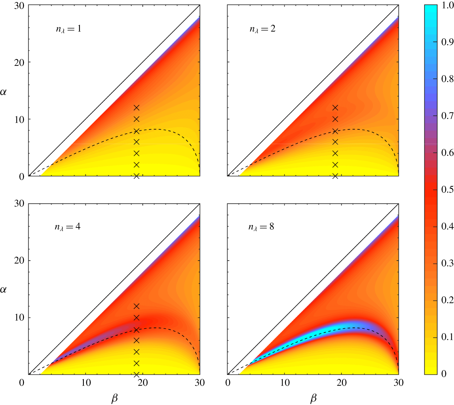
Figure 2 displays  $R^{th}$ in a
 $(\unicode[STIX]{x1D6FC},\unicode[STIX]{x1D6FD})$ diagram for
 $\unicode[STIX]{x1D6FE}=0$ (no rotation),
 $Fr=0.005$ and for four different values of
 $n_{\unicode[STIX]{x1D706}}$ equal to 1, 2, 4 and 8. These values, except for
 $n_{\unicode[STIX]{x1D706}}=8$, are those of the numerical simulations reported in § 4. The location of resonant triads, given by
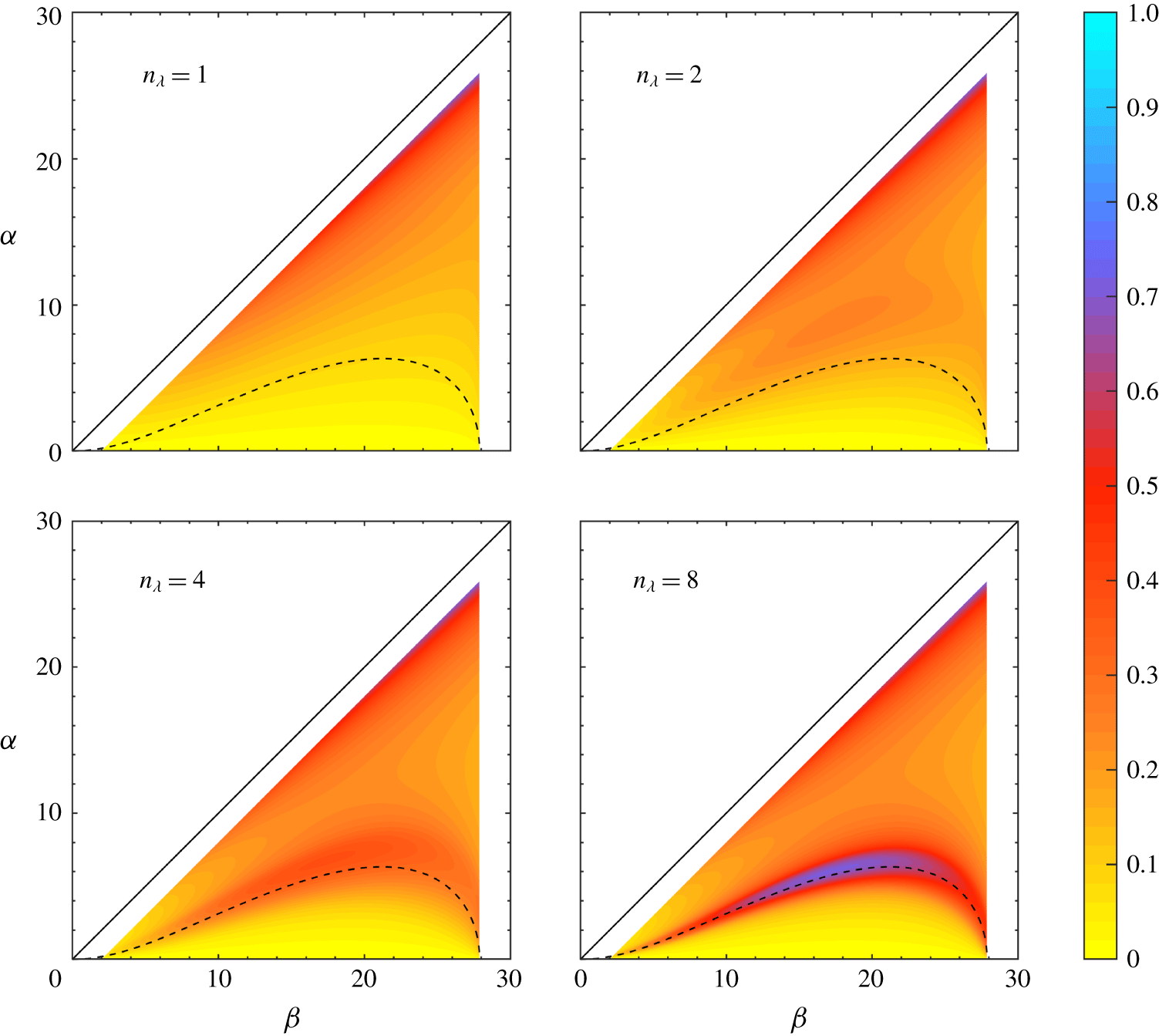
 $D=0$, is marked with a dashed curve. The counterpart diagram for
 $\unicode[STIX]{x1D6FE}=0.2$ is displayed in figure 3. Both figures show that, even if the Froude number is quite low and
 $n_{\unicode[STIX]{x1D706}}$ is at most equal to
 $8$,
 $R^{th}$ reaches values close to unity at resonance. Figure 2 also shows that, for small values of
 $n_{\unicode[STIX]{x1D706}}$, the location of resonant triads differs from the location where
 $R^{th}$ reaches a maximum value, the latter location superimposing on the former as
 $n_{\unicode[STIX]{x1D706}}$ grows. In other words, we recover TH87 prediction in the limit of pure plane waves. This result is confirmed in figure 8, further discussed in § 4, where
 $R^{th}$ (blue curve) is plotted versus
 $\unicode[STIX]{x1D6FC}$ for
 $n_{\unicode[STIX]{x1D706}}=1,2$ and 4 and for
 $\unicode[STIX]{x1D6FD}=18.9^{\circ }$: for
 $n_{\unicode[STIX]{x1D706}}\geqslant 2$,
 $R^{th}$ displays a maximum value which is all the more pronounced
 $n_{\unicode[STIX]{x1D706}}$ is larger; when
 $n_{\unicode[STIX]{x1D706}}$ increases, this maximum is reached for a value of
 $\unicode[STIX]{x1D6FC}$ that approaches the theoretical value at which resonance occurs for a pure plane wave.
Figure 3 shows that rotation does not qualitatively modify the resonance process, only making this maximum lower than in the non-rotating case. This behaviour can be explained with equation (2.20): the influence of rotation effects in the second-harmonic streamfunction amplitude at resonance only comes into play through the frequency  $\unicode[STIX]{x1D714}$ in the denominator of the expression of
 $\unicode[STIX]{x1D713}_{2}^{h}$. All parameters being kept the same, adding rotation increases
 $\unicode[STIX]{x1D714}$ and therefore lowers the second-harmonic amplitude.
Second-harmonic to first-order streamfunction norms  $R^{th}$, defined by (3.8), as a function of the slope angle
 $\unicode[STIX]{x1D6FC}$ and incidence angle
 $\unicode[STIX]{x1D6FD}$, for increasing width of the incident wave defined by the number of wavelengths
 $n_{\unicode[STIX]{x1D706}}$ it contains. For all panels, the Froude number
 $Fr=0.005$ and
 $f=0$ (no rotation). The dashed curve corresponds to the resonance condition
 $D=0$ for a pure plane wave (
 $n_{\unicode[STIX]{x1D706}}\rightarrow +\infty$), with
 $D$ defined by (2.15). The crosses refer to numerical simulations reported in § 4. The domain is limited to
 $\unicode[STIX]{x1D6FD}\leqslant 30^{\circ }$ because the second-harmonic free wave becomes evanescent above this range. Values of
 $R^{th}$ are also not plotted when approaching the critical case
 $\unicode[STIX]{x1D6FC}=\unicode[STIX]{x1D6FD}$ which is beyond the scope of this article.

Same as figure 2, for a ratio of the Coriolis frequency to the Brunt–Väisälä frequency equal to  $0.2$.

4 Comparison with numerical simulations
In order to estimate the validity of the theoretical predictions exposed in the previous section, two-dimensional numerical simulations in a vertical plane have been performed. As just discussed, including rotation does not qualitatively change the results so that the non-rotating case is considered in the present section. All quantities below are dimensional but we keep the same notation as before for the variables and parameters, for simplicity. In the following, the first-order solution, namely the superposition of the incident and reflected waves, will also be referred to as the first-harmonic wave.
4.1 Numerical configuration
The simulations were performed with the numerical model ‘Non-hydrostatic Ocean model for Earth Simulator’ (NHOES) which solves the free-surface non-hydrostatic Boussinesq equations in a Cartesian coordinate system (Aiki & Yamagata Reference Aiki and Yamagata2004). For the present study, equations (2.1) were solved with a viscous term  $\unicode[STIX]{x1D708}\unicode[STIX]{x1D6FB}^{2}\boldsymbol{u}$ added to the right-hand side of (2.1a) and a diffusive term
 $\unicode[STIX]{x1D705}\unicode[STIX]{x1D6FB}^{2}b$ to that of equation (2.1b);
 $\unicode[STIX]{x1D708}$ and
 $\unicode[STIX]{x1D705}$ are the kinematic viscosity and the diffusivity of buoyancy, respectively. The equation of state is linear and only depends on salinity. The choice of salinity rather than temperature is dictated by laboratory experiments conducted in parallel to the present study on the Coriolis platform at Grenoble in which density variations are created by a vertical profile of salt concentration. The viscosity is thus equal to
 $\unicode[STIX]{x1D708}=10^{-6}~\text{m}~\text{s}^{-1}$, namely that of water, while the diffusivity is set to
 $1.49\times 10^{-9}~\text{m}^{2}~\text{s}^{-1}$ since the Prandtl number of salt dissolved in water is approximately
 $700$. No sub-grid scale parametrization is used. The background stratification is linear, with a value of the Brunt–Väisälä frequency equal to
 $0.46~\text{s}^{-1}$ and, as said above, the Coriolis frequency
 $f$ is set to 0. These values and all values of the physical and geometrical parameters below are those of the laboratory experiments.
The numerical set-up is sketched in figure 1. The domain dimensions are 3 m in the horizontal direction and 0.8 m in the vertical direction. The bottom boundary condition is of the free-slip type and an implicit free-surface boundary condition is imposed at the top of the domain. The origin of the vertical axis, oriented positively upwards, is taken at the free surface.
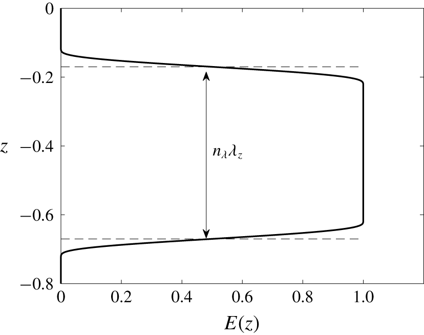
An internal gravity wave of finite vertical width is continuously forced at the left boundary of the numerical domain ( $x=0$) by adding a forcing function to the right-hand side of the momentum equation for the
 $u$-component (see figure 4),
 $$\begin{eqnarray}F_{x}(0,z,t)=UE(z)\left((1-\text{e}^{-5t/T})\,\unicode[STIX]{x1D714}\sin (k_{z}z-\unicode[STIX]{x1D714}t)+\left(\frac{5t}{T}\right)\text{e}^{-5t/T}\cos (k_{z}z-\unicode[STIX]{x1D714}t)\right)\end{eqnarray}$$
with
 $$\begin{eqnarray}E(z)=\frac{1}{2}\left(1+\tanh \left(\frac{3}{2}\tan \left(-\frac{\unicode[STIX]{x03C0}}{2}+\frac{1}{2}\min (2\unicode[STIX]{x03C0},\max (0,\unicode[STIX]{x03C0}(n_{\unicode[STIX]{x1D706}}+1)-k_{z}|z-z_{0}|))\right)\right)\right),\end{eqnarray}$$
where  $U$ is the velocity amplitude of the forcing,
 $\unicode[STIX]{x1D714}$ the wave frequency (and
 $T$ the wave period) and
 $k_{z}$ is the vertical wavenumber. This forcing generates the
 $u$-component of the incident plane wave. The smooth envelope in the
 $z$-direction
 $E(z)$ is centred at
 $z_{0}=-0.42~\text{m}$. The value of the frequency is equal to
 $0.149~\text{rad}~\text{s}^{-1}$, implying that the propagation angle of the incident wave
 $\unicode[STIX]{x1D6FD}=18.9^{\circ }$. The value of the vertical wavelength
 $\unicode[STIX]{x1D706}_{z}$ is 0.125 m, implying that the wavelength
 $\unicode[STIX]{x1D706}$ is equal to 0.118 m; four wavelengths are therefore permitted at most in the incident wave. The slope angle
 $\unicode[STIX]{x1D6FC}$ varies from
 $0^{\circ }$ to
 $12^{\circ }$. The value of
 $\unicode[STIX]{x1D6FC}$ at which resonance theoretically occurs in this case, referred to as
 $\unicode[STIX]{x1D6FC}_{\text{res}}$, is equal to
 $7.848^{\circ }$. The horizontal velocity amplitude is set to
 $U=3\times 10^{-4}~\text{m}~\text{s}^{-1}$. With these values, the Froude number of the incident wave
 $Fr=5\times 10^{-3}\ll 1$, which satisfies the condition for resonant interaction to occur. The corresponding value of the wave steepness is
 $s=0.034$.
A sponge layer of width 0.5 m is added at the right boundary in order to prevent wave reflection. The horizontal and vertical resolutions are equal to  $1.25\times 10^{-3}~\text{m}$ and
 $0.625\times 10^{-3}~\text{m}$, respectively. The latter value has been chosen so that the height
 $h$ of the interaction triangle between the incident and reflected waves, which decreases as
 $\unicode[STIX]{x1D6FC}$ increases, contains approximately 20 grid points for the largest value of
 $\unicode[STIX]{x1D6FC}$ we consider (equal to
 $12^{\circ }$). This vertical resolution implies that the vertical wavelength
 $\unicode[STIX]{x1D706}_{z}$ is described by 200 grid points.
Envelope function  $E(z)$ given by (4.1b). The vertical width of the incident wave is equal to
 $n_{\unicode[STIX]{x1D706}}\unicode[STIX]{x1D706}_{z}$ where
 $\unicode[STIX]{x1D706}_{z}$ is the vertical wavelength. The width of the wave is defined by the number of wavelengths
 $n_{\unicode[STIX]{x1D706}}$ contained in the envelope.

4.2 Results of the numerical simulations
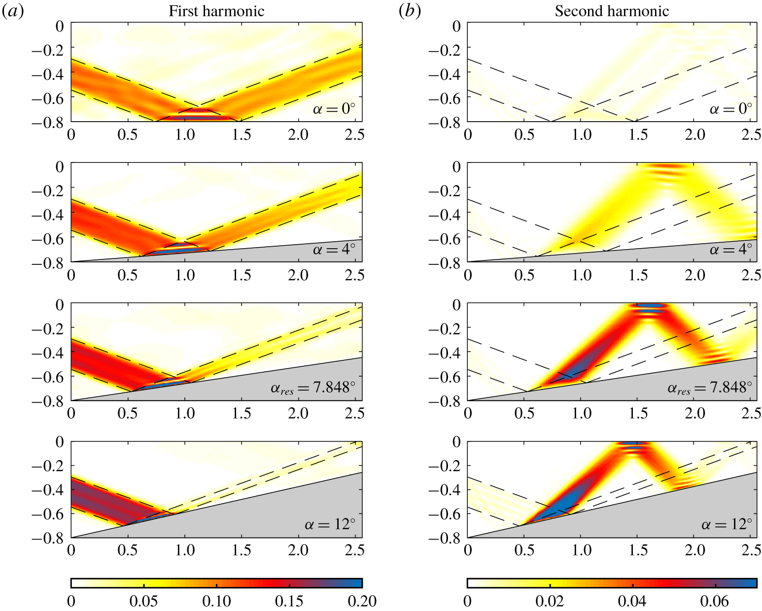
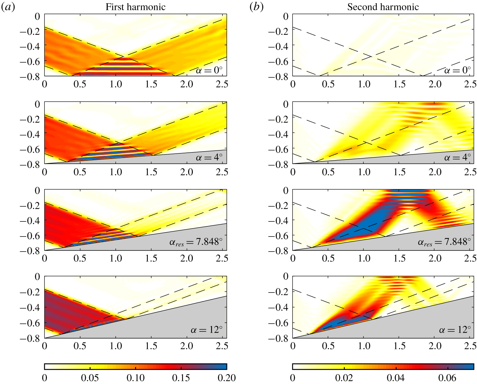
As indicated by the crosses in figure 2, numerical simulations have been performed for three different widths of the incident wave ( $n_{\unicode[STIX]{x1D706}}=1$, 2 and 4) and seven slope angles, equal to
 $0^{\circ }$,
 $2^{\circ }$,
 $4^{\circ }$,
 $6^{\circ }$,
 ${\unicode[STIX]{x1D6FC}_{res}=7.848}^{\circ }$,
 $10^{\circ }$ and
 $12^{\circ }$. Each simulation has been carried out over 40 wave periods.
The off-slope velocity (normal to the slope)  $w^{\prime }=-\unicode[STIX]{x2202}\unicode[STIX]{x1D713}/\unicode[STIX]{x2202}x^{\prime }$, filtered at either the incident wave frequency, denoted
 $w_{1}^{\prime }$, or twice this frequency, denoted
 $w_{2}^{\prime }$, is displayed for
 $n_{\unicode[STIX]{x1D706}}=2$ and
 $n_{\unicode[STIX]{x1D706}}=4$ in figures 5 and 6, respectively. The harmonic filtering has been performed over the last
 $8$ periods of the simulations. The choice of the
 $w^{\prime }$ variable is dictated by the forthcoming comparison with the theoretical predictions presented in the previous section.
Amplitude of the off-slope velocity component in  $\text{mm}~\text{s}^{-1}$ in the (
 $x$,
 $z$) plane, filtered at the first-harmonic frequency
 $\unicode[STIX]{x1D714}$ (left column) and at the second-harmonic frequency
 $2\,\unicode[STIX]{x1D714}$ (right column) for four different slope angles
 $\unicode[STIX]{x1D6FC}$;
 $\unicode[STIX]{x1D6FC}_{res}=7.848^{\circ }$ is the angle at which resonance occurs. The angle of incidence
 $\unicode[STIX]{x1D6FD}$ is constant and equal to
 $18.9^{\circ }$. The incident and reflected waves are delineated with dashed lines. The unit of the horizontal and vertical axes is in m. The envelope of the incident wave contains two wavelengths (
 $n_{\unicode[STIX]{x1D706}}=2$).

Same as figure 5 for an incident wave envelope containing four wavelengths ( $n_{\unicode[STIX]{x1D706}}=4$).

4.2.1 First-harmonic wave
We first consider the incident wave component  $w_{1}^{\prime }$ displayed in figures 5(a) and 6(a). Note that
 $w_{1}^{\prime }$ is proportional to
 $k$ by definition, namely to
 $|\boldsymbol{k}|\sin (\unicode[STIX]{x1D6FC}+\unicode[STIX]{x1D6FD})$.
Before entering the interaction area, the amplitude of  $w_{1}^{\prime }$ grows with
 $\unicode[STIX]{x1D6FC}$, since
 $|\boldsymbol{k}|$ and
 $\unicode[STIX]{x1D6FD}$ are kept fixed in all simulations. Figures 5(b) and 6(b) show that very weak amplitude second-harmonic waves are radiated from the forcing boundary of the incident wave due to the modulation of this wave by the envelope function (4.1b).
The incident and reflected waves superpose in the interaction area and the resulting streamfunction is given by (3.2). This equation implies that the  $\unicode[STIX]{x1D714}$-filtered interaction pattern does not vary along
 $x^{\prime }$ and has a sinusoidal dependency in
 $z^{\prime }$, as confirmed by figures 5(a) and 6(a), with wavenumber
 $k(n_{I}-n_{R})/2$.
Figures 5(a) and 6(a) however display a major feature, which is not accounted for in the theory. The theory assumes indeed that the off-slope velocity amplitude of the reflected wave is uniform and equal to that of the incident wave to satisfy the impermeability condition at the sloping boundary. While this is the case in the interaction area, at least close to the sloping boundary, the figures actually show that this amplitude is much weaker than that of the incident wave outside the interaction area, all the more so the slope angle is larger.
This behaviour has two origins. The first one is related to the focusing of the reflected wave and is due to molecular effects. The wavelength of the reflected wave, equal to  $\unicode[STIX]{x1D706}\sin (\unicode[STIX]{x1D6FD}-\unicode[STIX]{x1D6FC})/\sin (\unicode[STIX]{x1D6FD}+\unicode[STIX]{x1D6FC})$, is indeed smaller than the incident wavelength
 $\unicode[STIX]{x1D706}$ so that the viscous (or diffusive) time scale is smaller for the reflected wave as well. When scaled by the incident wave period, the viscous time scale decays from 16.8 to 0.9 as
 $\unicode[STIX]{x1D6FC}$ increases from
 $0^{\circ }$ to
 $12^{\circ }$. Dissipation thus becomes an important effect in the dynamics of the reflected wave as
 $\unicode[STIX]{x1D6FC}$ increases. The second effect is due to energy transfer to higher-harmonic waves. Figures 5(b) and 6(b) show that, as
 $\unicode[STIX]{x1D6FC}$ increases, the amplitude of the second-harmonic wave becomes no longer small compared to the amplitude of the incident wave. There is therefore a significant energy flux from the first-harmonic wave to the second-harmonic one which also reduces the amplitude of the reflected wave. Theoretical estimates of the power of the first-harmonic wave lost by dissipation and transferred to the second-harmonic wave are provided in § 5.
4.2.2 Second-harmonic wave
As discussed in the Introduction, when a finite-width plane wave incident on a flat surface interacts with the reflected wave, harmonic waves of frequency  $n\,\unicode[STIX]{x1D714}<N$ are generated. Figures 5(b) and 6(b) show indeed that a (weak amplitude) second-harmonic wave propagates from the interaction area for
 $\unicode[STIX]{x1D6FC}=0$. In the present case, only harmonics 2 and 3 can be generated with
 $3\,\unicode[STIX]{x1D714}=0.447$ very close to
 $N$, so that energy is dominantly transferred to the second-harmonic wave.
When  $\unicode[STIX]{x1D6FC}$ is non-zero, the second-harmonic wave field
 $\unicode[STIX]{x1D713}_{2}^{h}$ is the sum of a forced and a free wave, as discussed in § 2.3. The forced wave exists only in the interaction area between the incident and reflected waves. While being also generated inside the interaction area, the free wave can radiate away from this area. At resonance, the forced and free waves coincide (namely
 $m_{2}=n_{I}+n_{R}$, see (2.14)) and the amplitude of
 $\unicode[STIX]{x1D713}_{2}^{h}$ grows linearly with the normal to the slope
 $z^{\prime }$, the maximum value being reached at the top of the interaction area, for
 $z^{\prime }=h$.
Figures 5(b) and 6(b) show that, for  $\unicode[STIX]{x1D6FC}\neq 0$, the second-harmonic free wave is clearly visible outside the interaction area, with amplitude close to that area equal to that at the boundary of this area. This amplitude is largest for
 $\unicode[STIX]{x1D6FC}=\unicode[STIX]{x1D6FC}_{res}$, as expected. It is damped by dissipative effects as the free wave travels to the upper boundary where it reflects. Focusing now on the interaction area, figures 5(b) and 6(b) show that the amplitude of
 $w_{2}^{\prime }$ does not vary along the slope, as predicted by (2.17). This is visible for
 $\unicode[STIX]{x1D6FC}=\unicode[STIX]{x1D6FC}_{res}$ and
 $\unicode[STIX]{x1D6FC}=12^{\circ }$, and not so clearly for
 $\unicode[STIX]{x1D6FC}=4^{\circ }$, consistent with figure 2 showing that the second-harmonic amplitude is much weaker for
 $\unicode[STIX]{x1D6FC}=4^{\circ }$ than for the former angles. The behaviour of
 $w_{2}^{\prime }$ normal to the slope at resonance is analysed in the next section.
4.3 Comparison with the theoretical predictions
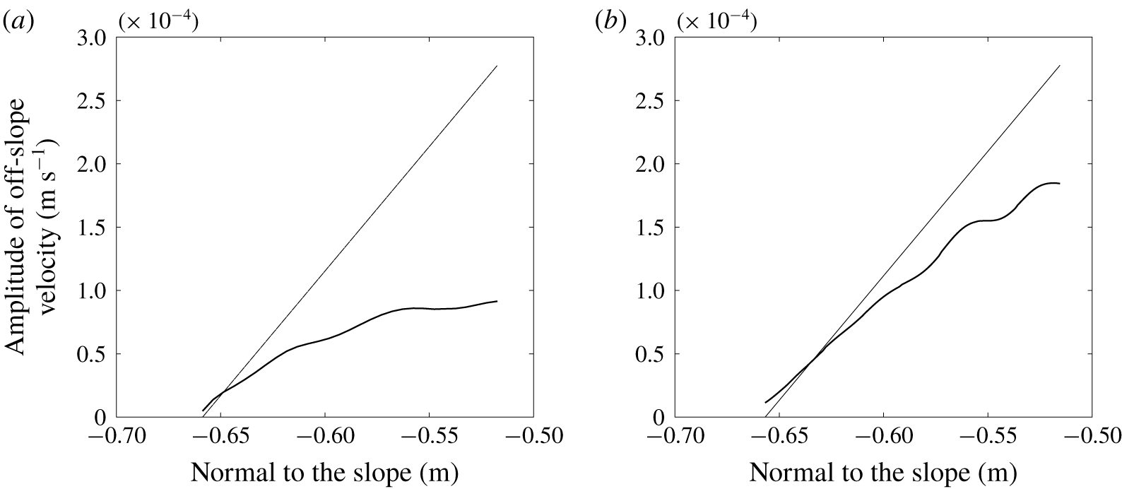
According to (2.20), in the absence of fluid viscosity, the amplitude of  $\unicode[STIX]{x1D713}_{2}^{h}$ evolves linearly with
 $z^{\prime }$ at resonance. To assess the validity of this theoretical prediction, this linear law is compared to the behaviour normal to the slope of the amplitude of
 $w_{2}^{\prime }$ inside the interaction area (
 $0\leqslant z^{\prime }\leqslant h$) for the simulation with
 $\unicode[STIX]{x1D6FC}=\unicode[STIX]{x1D6FC}_{res}$ and
 $n_{\unicode[STIX]{x1D706}}=4$ (see figure 7a). A poor agreement is obtained. Since the height
 $h$ is fairly well resolved in the numerical simulation (by more than 100 grid points), this discrepancy should be due to the assumption that the first-harmonic wave amplitude is constant in the theory, while dissipation and energy transfer decrease that amplitude in the simulation. As shown in § 5, dissipation is much larger than energy transfer in this simulation. The numerical simulation was therefore rerun with a ten times lower viscosity, namely
 $\unicode[STIX]{x1D708}=10^{-7}~\text{m}^{2}~\text{s}^{-1}$. The comparison is displayed in figure 7(b): the agreement has improved as the amplitude now grows linearly. The growth rate is still smaller than predicted, by approximately 30 %, a discrepancy mainly attributable to the decay of the first-harmonic wave amplitude through energy transfer to the second-harmonic wave (see § 5).
Amplitude of the second-harmonic off-slope velocity component at resonance computed by the numerical simulations, as a function of the coordinate normal to the slope ( $z^{\prime }$) in the interaction area for
 $n_{\unicode[STIX]{x1D706}}=4$,
 $\unicode[STIX]{x1D6FC}=\unicode[STIX]{x1D6FC}_{res}$, for two different values of fluid viscosity (a)
 $\unicode[STIX]{x1D708}=10^{-6}~\text{m}^{2}~\text{s}^{2}$, and (b)
 $\unicode[STIX]{x1D708}=10^{-7}~\text{m}^{2}~\text{s}^{2}$. The straight solid line is the theoretical prediction based on (2.20).

To further compare the numerical results with the theoretical predictions, the ratio  $R^{th}$ defined by (3.1) is compared with its numerical counterpart, denoted
 $R^{num}$. Rewriting
 $R^{th}$ as
 $$\begin{eqnarray}R^{th}=\frac{Fr}{2}\frac{2k\Vert \unicode[STIX]{x1D713}_{2}^{h}\Vert }{k\Vert \unicode[STIX]{x1D713}_{1}\Vert }=\frac{Fr}{2}\frac{\Vert \unicode[STIX]{x2202}_{{x^{\prime }}^{}}\unicode[STIX]{x1D713}_{2}^{h}\Vert }{\Vert \unicode[STIX]{x2202}_{{x^{\prime }}^{}}\unicode[STIX]{x1D713}_{1}\Vert },\end{eqnarray}$$
 $R^{num}$ can be defined as, in dimensional form,
 $$\begin{eqnarray}R^{num}=\frac{1}{2}\frac{\Vert w_{2}^{\prime }\Vert }{\Vert w_{1}^{\prime }\Vert }.\end{eqnarray}$$
The norm of the first- and second-harmonic off-slope velocities  $\Vert w_{1}^{\prime }\Vert$ and
 $\Vert w_{2}^{\prime }\Vert$ are defined by the maximum of their respective amplitude over the interaction area.
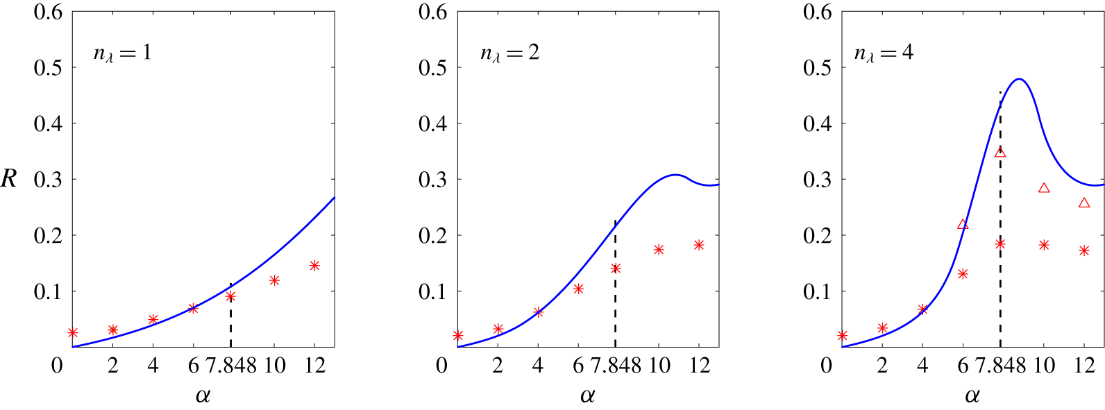
The ratio  $R^{th}$ is displayed in figure 8 for
 $n_{\unicode[STIX]{x1D706}}=1$, 2 and 4. As discussed in § 3,
 $R^{th}$ displays a maximum for
 $n_{\unicode[STIX]{x1D706}}\geqslant 2$, which grows with
 $n_{\unicode[STIX]{x1D706}}$ and is reached for a value of
 $\unicode[STIX]{x1D6FC}$ approaching
 $\unicode[STIX]{x1D6FC}_{res}$ as
 $n_{\unicode[STIX]{x1D706}}$ increases.
The ratio  $R^{num}$ is compared to
 $R^{th}$ in figure 8 (star symbols). For
 $\unicode[STIX]{x1D6FC}=0$, as expected, their values do not match since no harmonic wave is produced by the interaction of pure plane incident and reflected waves (so that
 $R^{th}=0$) while a harmonic wave is generated when these plane waves are of finite thickness (implying that
 $R^{num}\neq 0$). When
 $\unicode[STIX]{x1D6FC}$ has a non-zero value, figure 8 shows that the simulations are in good agreement with the theory for the lowest angles only, up to
 $\unicode[STIX]{x1D6FC}=\unicode[STIX]{x1D6FC}_{res}$ for
 $n_{\unicode[STIX]{x1D706}}=1$ and up to
 $\unicode[STIX]{x1D6FC}=4^{\circ }$ for
 $n_{\unicode[STIX]{x1D706}}=2$ and
 $n_{\unicode[STIX]{x1D706}}=4$. This can be explained as follows. The maximum theoretical amplitude of the first-harmonic wave is always reached in the simulations, but in the bottom part of the interaction area where the reflected wave has not been damped yet. The agreement with the theory (namely with
 $R^{th}$) therefore requires the theoretical maximum for the second-harmonic wave to be reached in the simulation. This theoretical maximum occurs at the top of the interaction area. In the simulation,
 $\Vert w_{2}^{\prime }\Vert$ will also be reached at that location if the amplitude of the reflected wave has hardly decayed in the interaction area. This occurs for small slope angles. For larger slope angles, the amplitude of the reflected wave has already weakened when reaching the top of the interaction area (mainly because of dissipation due to the strong focusing), leading to a weaker amplitude of the second-harmonic wave at that location than predicted.
The major role of viscosity in damping the reflected wave inside the interaction area is attested again by comparing the results of the theoretical predictions with those of the simulation with  $\unicode[STIX]{x1D708}=10^{-7}~\text{m}^{2}~\text{s}^{-1}$, for
 $n_{\unicode[STIX]{x1D706}}=4$ and
 $\unicode[STIX]{x1D6FC}\geqslant 6^{\circ }$. Results are plotted in figure 8 (triangle symbols) and show that the agreement with the theory has strongly improved. The departure from the theoretical predictions is mainly attributable to energy transfer to the second-harmonic wave, as noted above.
Comparison of the weakly nonlinear theory presented in § 3 with numerical simulations. The Froude number of the incident wave is  $Fr=5\times 10^{-3}$, the angle of incidence is
 $\unicode[STIX]{x1D6FD}=18.9^{\circ }$ and an incident wave with three different widths is considered:
 $n_{\unicode[STIX]{x1D706}}=1$, 2 and 4. The solid blue line is the theoretical ratio
 $R^{th}$ defined by (3.1) (expression (3.8) is plotted here). Its numerical counterpart
 $R^{num}$ defined by (4.3) is represented with symbols: stars for simulations with
 $\unicode[STIX]{x1D708}=10^{-6}~\text{m}^{2}~\text{s}^{-1}$ and triangles for
 $\unicode[STIX]{x1D708}=10^{-7}~\text{m}^{2}~\text{s}^{-1}$. The dashed line indicates the value of
 $\unicode[STIX]{x1D6FC}$ for which resonance is predicted by the theory of TH87.

5 Theoretical estimate of the energy budget
In order to estimate the relative importance of the damping processes of the first-harmonic wave, we determine in this section the power lost in the interaction area  $\unicode[STIX]{x1D6FA}$ by that wave due either to energy transfer to the second-harmonic wave or to dissipation and compare both powers to the incident energy flux. All results are obtained from the weakly nonlinear theory presented in § 2 in which dissipative effects are now introduced, with the first-order and second-order solutions derived in § 3.
We start from the general governing equations (2.1a) and (2.1b), which we write in non-dimensional form (keeping again the same notation for the parameters  $f$ and
 $N$, otherwise equal to
 $f/N$ and 1),
 $$\begin{eqnarray}\displaystyle & \displaystyle \frac{\unicode[STIX]{x2202}^{}}{\unicode[STIX]{x2202}t^{}}\boldsymbol{u}+\unicode[STIX]{x1D735}p+f\boldsymbol{e}_{z}\times \boldsymbol{u}-b\,\boldsymbol{e}_{z}=-Fr\,(\boldsymbol{u}\boldsymbol{\cdot }\unicode[STIX]{x1D735})\boldsymbol{u}, & \displaystyle\end{eqnarray}$$
 $$\begin{eqnarray}\displaystyle & \displaystyle \frac{\unicode[STIX]{x2202}^{}}{\unicode[STIX]{x2202}t^{}}b+N^{2}w=-Fr\,\boldsymbol{u}\boldsymbol{\cdot }\unicode[STIX]{x1D735}b. & \displaystyle\end{eqnarray}$$
 $$\begin{eqnarray}\displaystyle & \displaystyle \frac{\unicode[STIX]{x2202}^{}}{\unicode[STIX]{x2202}t^{}}\boldsymbol{u}_{1}+\unicode[STIX]{x1D735}p_{1}+f\boldsymbol{e}_{z}\times \boldsymbol{u}_{1}-b_{1}\,\boldsymbol{e}_{z}=0, & \displaystyle\end{eqnarray}$$
 $$\begin{eqnarray}\displaystyle & \displaystyle \frac{\unicode[STIX]{x2202}^{}}{\unicode[STIX]{x2202}t^{}}b_{1}+N^{2}w_{1}=0. & \displaystyle\end{eqnarray}$$
The usual operation  $\boldsymbol{u}_{1}\boldsymbol{\cdot }(5.2a)+(b_{1}/N^{2})(5.2b)$ yields the conservation equation for the total energy of the first-harmonic wave,
 $$\begin{eqnarray}\frac{\unicode[STIX]{x2202}^{}}{\unicode[STIX]{x2202}t^{}}E_{1}+\unicode[STIX]{x1D735}\boldsymbol{\cdot }\left(p_{1}\boldsymbol{u}_{1}\right)=0,\end{eqnarray}$$
with  $E_{1}=\frac{1}{2}(\boldsymbol{u}_{1}^{2}+b_{1}^{2}/N^{2})$.
Following the same steps at second order yields the energy equation
 $$\begin{eqnarray}\frac{\unicode[STIX]{x2202}^{}}{\unicode[STIX]{x2202}t^{}}E_{2}+\unicode[STIX]{x1D735}\boldsymbol{\cdot }\left(p_{2}\boldsymbol{u}_{2}\right)=-Fr^{2}\left[((\boldsymbol{u}_{1}\boldsymbol{\cdot }\unicode[STIX]{x1D735})\boldsymbol{u}_{1})\boldsymbol{\cdot }\boldsymbol{u}_{2}+\frac{1}{N^{2}}(\boldsymbol{u}_{1}\boldsymbol{\cdot }\unicode[STIX]{x1D735}b_{1})b_{2}\right].\end{eqnarray}$$
The right-hand side of the equation is the transfer term from the first-harmonic wave to the second-order solution. This second-order solution contains the second-harmonic wave plus an Eulerian mean flow. This mean flow does not radiate any wave so that, when the transfer term from the first-harmonic to the second-harmonic wave power density is sought, it does not come into play in this term. The latter term, denoted  $tp_{12}$, can therefore be written as
 $$\begin{eqnarray}tp_{12}=-Fr^{2}\left[((\boldsymbol{u}_{1}\boldsymbol{\cdot }\unicode[STIX]{x1D735})\boldsymbol{u}_{1})^{h}\boldsymbol{\cdot }\boldsymbol{u}_{2}^{h}+\frac{1}{N^{2}}(\boldsymbol{u}_{1}\boldsymbol{\cdot }\unicode[STIX]{x1D735}b_{1})^{h}\,b_{2}^{h}\right],\end{eqnarray}$$
where the superscript  $h$ stands for the harmonic part. Note that for consistency, the nonlinear term involving the first-harmonic wave is also written with the superscript
 $h$ (despite it contains only wave components).
The transfer term of power involved in the energy budget of the second-harmonic wave over the interaction area  $\unicode[STIX]{x1D6FA}$ is
 $$\begin{eqnarray}TP_{12}=\iint _{\unicode[STIX]{x1D6FA}}\langle tp_{12}\rangle \,\text{d}x^{\prime }\,\text{d}z^{\prime },\end{eqnarray}$$
where  $\langle \cdot \rangle$ designates the average operator over one wave period. We refer the reader to appendix B for the expression of this term and detailed calculations.
This transfer term has been determined with the assumption that the first-harmonic wave is not influenced by the second-harmonic generation. In the same way, one can determine an estimate of the power of the first-harmonic wave lost by viscous dissipation (diffusive effects being very small) by adding a viscous term to the right-hand side of (5.2a) and assuming that the inviscid first-order solution still holds. In this framework, the first-harmonic power density lost by dissipation is given by
 $$\begin{eqnarray}dp_{1}=\frac{Fr}{Re}\,\unicode[STIX]{x1D735}\boldsymbol{u}_{1}:\unicode[STIX]{x1D735}\boldsymbol{u}_{1}=\frac{Fr}{Re}\,\Bigl[|{\unicode[STIX]{x1D735}u_{1}}^{2}|+|{\unicode[STIX]{x1D735}v_{1}}^{2}|+|{\unicode[STIX]{x1D735}w_{1}}^{2}|\Bigr],\end{eqnarray}$$
where  $Re=U\unicode[STIX]{x1D706}/\unicode[STIX]{x1D708}$ is the Reynolds number. As above, when the energy budget of the first-harmonic wave over
 $\unicode[STIX]{x1D6FA}$ is considered, an average operator over the wave period and over
 $\unicode[STIX]{x1D6FA}$ should be applied to
 $dp_{1}$ leading to
 $$\begin{eqnarray}DP_{1}=\iint _{\unicode[STIX]{x1D6FA}}\langle dp_{1}\rangle \,\text{d}x^{\prime }\,\text{d}z^{\prime }\end{eqnarray}$$
(see appendix B for the expression of this term and detailed calculations).
We finally need to compare the power of the first-harmonic wave lost into nonlinear transfer  $TP_{12}$ and dissipation
 $DP_{1}$ to the incident energy flux
 $$\begin{eqnarray}P_{I}=\int _{\unicode[STIX]{x2202}\unicode[STIX]{x1D6FA}}p_{I}\boldsymbol{u}_{I}\boldsymbol{\cdot }\text{d}\boldsymbol{n}=\int _{\unicode[STIX]{x2202}\unicode[STIX]{x1D6FA}}E_{I}\boldsymbol{c}_{gI}\boldsymbol{\cdot }\text{d}\boldsymbol{n},\end{eqnarray}$$
where the  $I$ subscript indicates the incident part of the first-harmonic wave,
 $\boldsymbol{c}_{g}$ is the group velocity,
 $\unicode[STIX]{x2202}\unicode[STIX]{x1D6FA}$ designates the boundary of the interaction area and
 $\text{d}\boldsymbol{n}$ the outgoing unit normal vector on
 $\unicode[STIX]{x2202}\unicode[STIX]{x1D6FA}$. The second equality in (5.9) holds only for a pure plane monochromatic wave. The reader is again referred to appendix A for its expression.
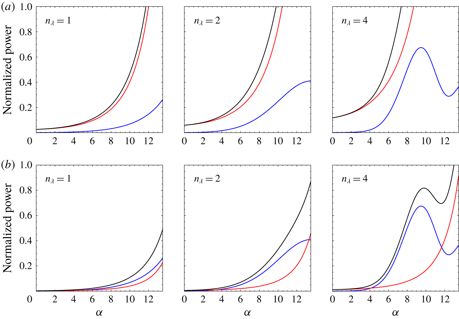
Energy budget for the first-harmonic wave in the interaction area  $\unicode[STIX]{x1D6FA}$ (yellow triangle in figure 1) as obtained from the weakly nonlinear theory in which dissipative effects have been added. The molecular viscosity is equal to
 $\unicode[STIX]{x1D708}=10^{-6}~\text{m}^{2}~\text{s}^{-1}$ in the first row and to
 $\unicode[STIX]{x1D708}=10^{-7}~\text{m}^{2}~\text{s}^{-1}$ in the second row. The blue and red curves represent the power averaged over one period transferred to the second-harmonic wave and dissipated by viscous effects, respectively, as a function of the slope angle
 $\unicode[STIX]{x1D6FC}$; each power is scaled by the incident energy flux in
 $\unicode[STIX]{x1D6FA}$. The black curve is the sum of the scaled powers. The fixed parameters are the incidence angle
 $\unicode[STIX]{x1D6FD}=18.9^{\circ }$ and the Froude number
 $Fr$ and Reynolds number
 $Re$ of the incident wave used in the numerical simulations;
 $Fr=5\times 10^{-3}$ and
 $Re$ is equal to 35 in the first row and to 350 in the second row.

The scaled powers  $TP_{12}/P_{I}$,
 $DP_{1}/P_{I}$ and their sum are shown in figure 9 for two different values of fluid viscosity,
 $\unicode[STIX]{x1D708}=10^{-6}~\text{m}^{2}~\text{s}^{-1}$ and
 $\unicode[STIX]{x1D708}=10^{-7}~\text{m}^{2}~\text{s}^{-1}$. It should first be noted that both
 $TP_{12}$ and
 $DP_{1}$ are overestimated as their expressions have been derived under the assumption that the first-harmonic wave is not influenced by second-harmonic transfer and dissipation (in particular, the lower amplitude of the reflected wave is not taken into account). The first-harmonic wave therefore behaves as an infinite energy source for the transfer and dissipation terms so that the scaled power ratios can exceed
 $1$. Figure 9 shows that, whatever the value of
 $\unicode[STIX]{x1D708}$, the dissipated power of the first-harmonic wave increases with
 $\unicode[STIX]{x1D6FC}$ because of the focusing of the reflected wave. For
 $\unicode[STIX]{x1D708}=10^{-6}~\text{m}^{2}~\text{s}^{-1}$ (figure 9a), the power lost by the first-harmonic wave is dominated by dissipation whatever
 $n_{\unicode[STIX]{x1D706}}$, even when resonance occurs (associated with a maximum of the transfer term). By contrast, when the value of fluid viscosity is lowered to
 $\unicode[STIX]{x1D708}=10^{-7}~\text{m}^{2}~\text{s}^{-1}$ (figure 9b), transfers to the second-harmonic wave are much higher than power lost by dissipation, up to
 $\unicode[STIX]{x1D6FC}\simeq 12^{\circ }$ or so. For a larger angle, the transfer term decreases while the impact of focusing on the reflected first-harmonic wave increases, promoting dissipation.
These power estimates confirm the previous statements that dissipation of the first-harmonic wave is the main process accounting for the discrepancy between  $R^{th}$ and
 $R^{num}$ for
 $\unicode[STIX]{x1D708}=10^{-6}~\text{m}^{2}~\text{s}^{-1}$, due to the focusing of the reflected wave. For a 10 times smaller viscosity, the departure from
 $R^{th}$ is mainly attributable to energy transfer to the second-harmonic wave.
These results imply that two-dimensional laboratory experiments (with water) cannot evaluate the validity of the TH87 theory, for a finite-width incident plane wave with the set of parameters we consider. The reason is that the Reynolds number of the incident wave  $Re=U\unicode[STIX]{x1D706}/\unicode[STIX]{x1D708}$, equal to 35, is too low. Decreasing
 $\unicode[STIX]{x1D708}$ by a factor 10 in the Reynolds number, as done in the simulations, is equivalent to increasing
 $U$ by a factor 10, suggesting that favourable conditions to test the TH87 theory could be achieved in the laboratory experiments. However, with
 $Fr$ increasing by a factor 10 as well, the regime is no longer weakly nonlinear since the incident wave steepness becomes equal to 0.34. The conditions to test the TH87 theory are therefore not met either. (Increasing the wavelength by a factor 10 would ensure both a higher Reynolds number and a lower Froude number but is not feasible in practice.)
6 Summary and conclusion
The purpose of this paper is to address the nonlinear reflection of a finite-width internal gravity wave incident on a uniform slope, away from critical incidence, in a two-dimensional vertical plane. The incident wave propagates against the slope, leading to focusing of the reflected wave. The paper has three objectives: (i) to revisit the inviscid and weakly nonlinear theory of TH87 when resonant conditions between an incident pure plane wave, the reflected wave and the second-harmonic wave, are met; at resonance indeed, the amplitude of the second-harmonic streamfunction is expressed as an indeterminate form leading to the common inference in the literature that this amplitude diverges; (ii) to apply this theory to an incident plane wave of finite width in the direction normal to wave propagation, as produced by the wave generator device commonly used in laboratory experiments to model plane-wave dynamics; (iii) to compare the latter theoretical predictions with results of two-dimensional numerical simulations of an incident plane wave of finite width.
We show that the indeterminacy at resonance can be waived and that the amplitude of the second-harmonic streamfunction is a linear function of the distance from the slope, consistent with a resonant forcing.
For an incident plane wave of finite width, which we model theoretically as a pure plane wave in a vertical plane with a finite number of wavelengths, the generation of second-harmonic waves is limited to the area where the incident and reflected waves superpose. The amplitude of the second-harmonic streamfunction is therefore now bounded. At resonance, its maximum value scaled by that of the first-harmonic wave increases with the number of wavelengths  $n_{\unicode[STIX]{x1D706}}$ and becomes close to
 $1$ for
 $n_{\unicode[STIX]{x1D706}}\geqslant 4$ even for a Froude number of the incident wave as small as 0.005. This implies that the reflection problem at resonance is highly nonlinear. We also showed that rotation does not qualitatively change the results, the second-harmonic wave amplitude being weaker when rotation is imposed. Numerical simulations of an incident plane wave of finite width were thus performed in the non-rotating case to estimate the validity of the theoretical predictions, for parameters of laboratory experiments performed in parallel to the present study. Slope angles up to
 $12^{\circ }$, still well below critical incidence (equal to
 $18.9^{\circ }$), and various incident wave widths were considered in the numerical simulations.
These simulations show that the amplitude of the reflected wave is damped for a sloping boundary, and more so when the slope angle is larger. For the highest angle we consider, almost no reflected wave leaves the interaction region. The main reason lies in the focusing of that wave, which enhances viscous dissipation. Because the first-harmonic wave amplitude is assumed to be constant in the theory, the numerical results differ from the theoretical predictions (for slope angles greater than a few degrees), a discrepancy mainly contributed by this damping process. Rerunning the numerical simulation with a 10 times smaller viscosity shows indeed that the amplitude of the second-harmonic wave agrees with the theoretical prediction to better than 20 %, the discrepancy being now attributable to the decay of the first-harmonic amplitude due to energy transfer. At resonance, the theoretical linear growth rate is recovered with an error of approximately 30 % with the 10 times smaller viscosity. These results can be made more precise by introducing dissipative effects in the weakly nonlinear theory. We show that, whatever the slope angle, the dissipated power of the primary wave is larger than the power transferred to the second-harmonic wave, accounting for the main discrepancy with the theory; when the viscosity is divided by a factor 10, the power lost by energy transfer dominates over the dissipated power.
These results imply that the validity of the theoretical predictions cannot be assessed by (quasi-) two-dimensional laboratory experiments in a vertical plane, because of the too low value of the incident wave Reynolds number (equal to 35 in the numerical simulations). Decreasing the value of the viscosity by a factor 10 in the simulations is equivalent to increasing the wave amplitude by the same factor in the laboratory experiments to keep the same Reynolds number. However the now 10 times larger Froude number implies that the incident wave would no longer be of weak amplitude in the experiments (its steepness being equal to 0.34) so that the assumptions of the TH87 theory are no longer satisfied.
The three-dimensional laboratory experiments conducted in parallel to the present two-dimensional numerical simulations are also not appropriate to test the theoretical predictions. Indeed a Lagrangian mean flow is induced in the interaction area as a result of nonlinear and dissipative effects, whose amplitude can be as large as that of the incident wave due to cumulative dissipative effect (Grisouard et al. Reference Grisouard, Leclair, Gostiaux and Staquet2013). As a result, the incident wave frequency is shifted through Doppler effect by the mean flow and refracted (with the phase lines bending toward the horizontal), which deeply modifies the incident wave geometry. This mean flow does not occur in a two-dimensional vertical plane because of the topography, which breaks the horizontal homogeneity required for the mean flow to develop. (This mean flow results from the same generation process as that induced by a single wave beam, as observed by Bordes et al. (Reference Bordes, Venaille, Joubaud and Odier2012) in their laboratory experiments, and theoretically modelled by Kataoka & Akylas (Reference Kataoka and Akylas2015).) Three-dimensional numerical simulations should therefore be performed for any comparison to be possible with the laboratory experiments. This joint approach has been carried out by the authors of the present paper and the analysis of the resulting nonlinear wave–slope interaction will be reported in a subsequent paper.
Acknowledgements
We thank N. Grisouard, L. Gostiaux, M.-P. Lelong and J. Sommeria for useful discussions and H. Aiki for his help in using the NHOES code. M.L. was supported by the ANR program and computations were performed at the French supercomputer centre of CINES.
Declaration of interests
The authors report no conflict of interest.
Appendix A. Weakly nonlinear second-order calculations
A.1 Computing the second-order solution
In this section we solve the linear partial differential equation (2.13). Using (2.8), (2.11) and (2.12), the right-hand side of (2.13a) becomes
 $$\begin{eqnarray}-12a_{1}^{2}k^{4}\unicode[STIX]{x1D714}\frac{s_{\unicode[STIX]{x1D6FD}}^{2}c_{\unicode[STIX]{x1D6FD}}^{2}s_{\unicode[STIX]{x1D6FC}}c_{\unicode[STIX]{x1D6FC}}}{\left(s_{\unicode[STIX]{x1D6FD}}^{2}-s_{\unicode[STIX]{x1D6FC}}^{2}\right)^{3}}\sin (\unicode[STIX]{x1D711}_{I}+\unicode[STIX]{x1D711}_{R})+4a_{1}^{2}k^{4}\frac{N^{2}s_{\unicode[STIX]{x1D6FC}}^{2}+f^{2}c_{\unicode[STIX]{x1D6FC}}^{2}}{\unicode[STIX]{x1D714}}\frac{s_{\unicode[STIX]{x1D6FD}}^{3}c_{\unicode[STIX]{x1D6FD}}^{3}}{\left(s_{\unicode[STIX]{x1D6FD}}^{2}-s_{\unicode[STIX]{x1D6FC}}^{2}\right)^{3}}\sin (\unicode[STIX]{x1D711}_{I}-\unicode[STIX]{x1D711}_{R}),\end{eqnarray}$$
where the simplified notations  $\unicode[STIX]{x1D711}_{I}=(kx^{\prime }+n_{I}kz^{\prime }-\unicode[STIX]{x1D714}t)$ and
 $\unicode[STIX]{x1D711}_{R}=(kx^{\prime }+n_{R}kz^{\prime }-\unicode[STIX]{x1D714}t)$ have been introduced. As expected, nonlinear terms computed for the first-order solution result in an oscillatory term of frequency
 $2\unicode[STIX]{x1D714}$ and a steady term. A particular solution of (2.13a) is therefore sought in the form
 $$\begin{eqnarray}\unicode[STIX]{x1D713}_{2}^{part}=a_{2}^{h}\sin (\unicode[STIX]{x1D711}_{I}+\unicode[STIX]{x1D711}_{R})+a_{2}^{s}\sin (\unicode[STIX]{x1D711}_{I}-\unicode[STIX]{x1D711}_{R}),\end{eqnarray}$$
the  $h$ and
 $s$ superscripts standing for harmonic and steady, respectively. The first term in (A 2) corresponds to the forced wave in TH87. Substituting expression (A 2) in (2.13a) yields
 $$\begin{eqnarray}a_{2}^{h}=\frac{3a_{1}^{2}k^{2}\unicode[STIX]{x1D714}}{D}\frac{s_{\unicode[STIX]{x1D6FD}}^{2}c_{\unicode[STIX]{x1D6FD}}^{2}s_{\unicode[STIX]{x1D6FC}}c_{\unicode[STIX]{x1D6FC}}}{s_{\unicode[STIX]{x1D6FD}}^{2}-s_{\unicode[STIX]{x1D6FC}}^{2}}\quad \text{and}\quad a_{2}^{s}=-\frac{a_{1}^{2}k^{2}}{\unicode[STIX]{x1D714}}\frac{s_{\unicode[STIX]{x1D6FD}}c_{\unicode[STIX]{x1D6FD}}}{s_{\unicode[STIX]{x1D6FD}}^{2}-s_{\unicode[STIX]{x1D6FC}}^{2}},\end{eqnarray}$$
where
 $$\begin{eqnarray}D=N^{2}s_{\unicode[STIX]{x1D6FD}}^{2}\left(4s_{\unicode[STIX]{x1D6FD}}^{4}-7s_{\unicode[STIX]{x1D6FD}}^{2}s_{\unicode[STIX]{x1D6FC}}^{2}+4s_{\unicode[STIX]{x1D6FC}}^{2}-s_{\unicode[STIX]{x1D6FD}}^{2}\right)+f^{2}c_{\unicode[STIX]{x1D6FD}}^{2}\left(4s_{\unicode[STIX]{x1D6FD}}^{4}-7s_{\unicode[STIX]{x1D6FD}}^{2}s_{\unicode[STIX]{x1D6FC}}^{2}+3s_{\unicode[STIX]{x1D6FC}}^{2}\right).\end{eqnarray}$$
This expression is in agreement with Thorpe (Reference Thorpe1997) (equation (7)).
Since the frequency and along-slope wavenumber of the second-harmonic motions are  $2\unicode[STIX]{x1D714}$ and
 $2k$, respectively, the solution of the homogeneous equation must be of the form
 $$\begin{eqnarray}\unicode[STIX]{x1D713}_{2}^{0}=a_{2}^{0}\sin \left(2kx^{\prime }+m_{2}kz^{\prime }-2\unicode[STIX]{x1D714}t+\unicode[STIX]{x1D711}_{2}^{0}\right),\end{eqnarray}$$
called the free wave in TH87. To ensure that this wave satisfies the dispersion relation and radiates energy away from the boundary,  $m_{2}$ must be defined by
 $$\begin{eqnarray}m_{2}=\frac{-2s_{\unicode[STIX]{x1D6FC}}c_{\unicode[STIX]{x1D6FC}}(N^{2}-f^{2})+2s_{\unicode[STIX]{x1D6FD}}\sqrt{4s_{\unicode[STIX]{x1D6FD}}^{4}N^{4}(1-4s_{\unicode[STIX]{x1D6FD}}^{2})+4c_{\unicode[STIX]{x1D6FD}}^{4}N^{4}(1-4c_{\unicode[STIX]{x1D6FD}}^{2})+N^{2}f^{2}(3-32s_{\unicode[STIX]{x1D6FD}}^{2}c_{\unicode[STIX]{x1D6FD}}^{2})}}{N^{2}(4s_{\unicode[STIX]{x1D6FD}}^{2}-s_{\unicode[STIX]{x1D6FC}}^{2})+f^{2}(4c_{\unicode[STIX]{x1D6FD}}^{2}-c_{\unicode[STIX]{x1D6FC}}^{2})}.\end{eqnarray}$$
Combining the particular and homogeneous solutions (A 2) and (A 5), the final solution of (2.13) is given by
 $$\begin{eqnarray}\displaystyle \unicode[STIX]{x1D713}_{2} & = & \displaystyle 3a_{1}^{2}k^{2}\unicode[STIX]{x1D714}\frac{s_{\unicode[STIX]{x1D6FD}}^{2}c_{\unicode[STIX]{x1D6FD}}^{2}s_{\unicode[STIX]{x1D6FC}}c_{\unicode[STIX]{x1D6FC}}}{(s_{\unicode[STIX]{x1D6FD}}^{2}-s_{\unicode[STIX]{x1D6FC}}^{2})D}[\sin (2kx^{\prime }+m_{2}kz^{\prime }-2\unicode[STIX]{x1D714}t)-\sin (2kx^{\prime }+(n_{I}+n_{R})kz^{\prime }-2\unicode[STIX]{x1D714}t)]\nonumber\\ \displaystyle & & \displaystyle -\,\frac{a_{1}^{2}k^{2}}{\unicode[STIX]{x1D714}}\frac{s_{\unicode[STIX]{x1D6FD}}c_{\unicode[STIX]{x1D6FD}}}{s_{\unicode[STIX]{x1D6FD}}^{2}-s_{\unicode[STIX]{x1D6FC}}^{2}}\sin ((n_{I}-n_{R})kz^{\prime }),\end{eqnarray}$$
where the constant parameters  $a_{2}^{0}=-a_{2}^{h}$ and
 $\unicode[STIX]{x1D711}_{2}^{0}=0$ have been determined through the boundary condition (2.13b).
Using (2.2b) and (2.2c), one can then derive the expressions of the harmonic parts of  $b_{2}$ and
 $v_{2}$, namely
 $$\begin{eqnarray}\displaystyle v_{2}^{h} & = & \displaystyle \frac{a_{1}^{2}fk^{3}s_{\unicode[STIX]{x1D6FD}}^{2}c_{\unicode[STIX]{x1D6FD}}^{2}c_{\unicode[STIX]{x1D6FC}}}{\left(s_{\unicode[STIX]{x1D6FD}}^{2}-s_{\unicode[STIX]{x1D6FC}}^{2}\right)^{2}(N^{2}s_{\unicode[STIX]{x1D6FD}}^{2}+f^{2}c_{\unicode[STIX]{x1D6FD}}^{2})}\sin (2kx^{\prime }+(n_{I}+n_{R})kz^{\prime }-2\unicode[STIX]{x1D714}t)\nonumber\\ \displaystyle & & \displaystyle -\,\frac{3a_{1}^{2}fk^{3}s_{\unicode[STIX]{x1D6FD}}^{2}c_{\unicode[STIX]{x1D6FD}}^{2}s_{\unicode[STIX]{x1D6FC}}^{2}c_{\unicode[STIX]{x1D6FC}}}{\left(s_{\unicode[STIX]{x1D6FD}}^{2}-s_{\unicode[STIX]{x1D6FC}}^{2}\right)D}[\sin (2kx^{\prime }+(n_{I}+n_{R})kz^{\prime }-2\unicode[STIX]{x1D714}t)-\sin (2kx^{\prime }+m_{2}kz^{\prime }-2\unicode[STIX]{x1D714}t)]\nonumber\\ \displaystyle & & \displaystyle -\,\frac{3a_{1}^{2}fk^{3}s_{\unicode[STIX]{x1D6FD}}^{2}c_{\unicode[STIX]{x1D6FD}}^{2}s_{\unicode[STIX]{x1D6FC}}c_{\unicode[STIX]{x1D6FC}}^{2}}{2\left(s_{\unicode[STIX]{x1D6FD}}^{2}-s_{\unicode[STIX]{x1D6FC}}^{2}\right)D}\left[(n_{I}+n_{R})\sin (2kx^{\prime }+(n_{I}+n_{R})kz^{\prime }-2\unicode[STIX]{x1D714}t)\right.\nonumber\\ \displaystyle & & \displaystyle \left.-\,m_{2}\sin (2kx^{\prime }+m_{2}kz^{\prime }-2\unicode[STIX]{x1D714}t)\right]\end{eqnarray}$$
and
 $$\begin{eqnarray}\displaystyle b_{2}^{h} & = & \displaystyle \frac{a_{1}^{2}N^{2}k^{3}s_{\unicode[STIX]{x1D6FD}}^{2}c_{\unicode[STIX]{x1D6FD}}^{2}s_{\unicode[STIX]{x1D6FC}}}{\left(s_{\unicode[STIX]{x1D6FD}}^{2}-s_{\unicode[STIX]{x1D6FC}}^{2}\right)^{2}(N^{2}s_{\unicode[STIX]{x1D6FD}}^{2}+f^{2}c_{\unicode[STIX]{x1D6FD}}^{2})}\sin (2kx^{\prime }+(n_{I}+n_{R})kz^{\prime }-2\unicode[STIX]{x1D714}t)\nonumber\\ \displaystyle & & \displaystyle -\,\frac{3a_{1}^{2}N^{2}k^{3}s_{\unicode[STIX]{x1D6FD}}^{2}c_{\unicode[STIX]{x1D6FD}}^{2}s_{\unicode[STIX]{x1D6FC}}c_{\unicode[STIX]{x1D6FC}}^{2}}{\left(s_{\unicode[STIX]{x1D6FD}}^{2}-s_{\unicode[STIX]{x1D6FC}}^{2}\right)D}[\sin (2kx^{\prime }+(n_{I}+n_{R})kz^{\prime }-2\unicode[STIX]{x1D714}t)-\sin (2kx^{\prime }+m_{2}kz^{\prime }-2\unicode[STIX]{x1D714}t)]\nonumber\\ \displaystyle & & \displaystyle -\,\frac{3a_{1}^{2}N^{2}k^{3}s_{\unicode[STIX]{x1D6FD}}^{2}c_{\unicode[STIX]{x1D6FD}}^{2}s_{\unicode[STIX]{x1D6FC}}^{2}c_{\unicode[STIX]{x1D6FC}}}{2\left(s_{\unicode[STIX]{x1D6FD}}^{2}-s_{\unicode[STIX]{x1D6FC}}^{2}\right)D}\left[(n_{I}+n_{R})\sin (2kx^{\prime }+(n_{I}+n_{R})kz^{\prime }-2\unicode[STIX]{x1D714}t)\right.\nonumber\\ \displaystyle & & \displaystyle \left.-\,m_{2}\sin (2kx^{\prime }+m_{2}kz^{\prime }-2\unicode[STIX]{x1D714}t)\right].\end{eqnarray}$$
Interestingly, as noted by Wunsch (Reference Wunsch1971) in a similar weakly nonlinear study of internal waves encountering a shoaling region, the system becomes degenerate when considering the steady problem in the presence of background rotation. The fields  $v_{2}^{s}$ and
 $b_{2}^{s}$ are indeed linked through the equation
 $$\begin{eqnarray}\frac{\unicode[STIX]{x2202}^{}}{\unicode[STIX]{x2202}x^{}}b_{2}^{s}-f\frac{\unicode[STIX]{x2202}^{}}{\unicode[STIX]{x2202}z^{}}v_{2}^{s}=J(\unicode[STIX]{x1D713}_{1},\unicode[STIX]{x1D6FB}^{2}\unicode[STIX]{x1D713}_{1})^{s},\end{eqnarray}$$
where the subscript  $s$ on the right-hand side refers to the steady component, but remain undetermined.
A.2 Determining the behaviour at resonance
In this section, we analyse the behaviour of  $\unicode[STIX]{x1D713}_{2}$ as
 $D\rightarrow 0$. The point is that
 $D$ appears in the denominator of (2.14) and the numerator also vanishes when
 $D\rightarrow 0$. One can indeed show that
 $$\begin{eqnarray}m_{2}=n_{I}+n_{R}\Leftrightarrow \left[N^{2}(4s_{\unicode[STIX]{x1D6FD}}^{2}-s_{\unicode[STIX]{x1D6FC}}^{2})+f^{2}(4c_{\unicode[STIX]{x1D6FD}}^{2}-c_{\unicode[STIX]{x1D6FC}}^{2})\right]D=0,\end{eqnarray}$$
so that  $D=0$ implies that the incident
 $(k,n_{I}k,\unicode[STIX]{x1D714})$, reflected
 $(k,n_{R}k,\unicode[STIX]{x1D714})$ waves and the second-harmonic free wave
 $(2k,m_{2}k,2\unicode[STIX]{x1D714})$ form a resonant triad.
A way to remove this indeterminacy is to reformulate the expression of  $\unicode[STIX]{x1D713}_{2}$ as (2.17). The following expression of
 $\unicode[STIX]{x1D6FF}=\frac{1}{2}(m_{2}-(n_{I}+n_{R}))$ is then obtained (from where (A 11) is inferred),
 $$\begin{eqnarray}\unicode[STIX]{x1D6FF}=\frac{3s_{\unicode[STIX]{x1D6FD}}^{2}s_{\unicode[STIX]{x1D6FC}}c_{\unicode[STIX]{x1D6FC}}}{(4s_{\unicode[STIX]{x1D6FD}}^{2}-s_{\unicode[STIX]{x1D6FC}}^{2})(s_{\unicode[STIX]{x1D6FD}}^{2}-s_{\unicode[STIX]{x1D6FC}}^{2})}\left[1-\sqrt{1-\frac{4s_{\unicode[STIX]{x1D6FD}}^{2}-s_{\unicode[STIX]{x1D6FC}}^{2}}{(3s_{\unicode[STIX]{x1D6FD}}s_{\unicode[STIX]{x1D6FC}}c_{\unicode[STIX]{x1D6FC}})^{2}}D}\right].\end{eqnarray}$$
This expression enables us to find the behaviour of  $\unicode[STIX]{x1D6FF}$ as
 $D\rightarrow 0$
 $$\begin{eqnarray}\unicode[STIX]{x1D6FF}\underset{D\rightarrow 0}{{\sim}}\frac{D}{6s_{\unicode[STIX]{x1D6FC}}c_{\unicode[STIX]{x1D6FC}}\left(s_{\unicode[STIX]{x1D6FD}}^{2}-s_{\unicode[STIX]{x1D6FC}}^{2}\right)}\end{eqnarray}$$
and the expression for the second-harmonic wave at resonance
 $$\begin{eqnarray}\unicode[STIX]{x1D713}_{2}^{h}=\frac{a_{1}^{2}k^{2}}{\unicode[STIX]{x1D714}}\frac{s_{\unicode[STIX]{x1D6FD}}^{2}c_{\unicode[STIX]{x1D6FD}}^{2}}{\left(s_{\unicode[STIX]{x1D6FD}}^{2}-s_{\unicode[STIX]{x1D6FC}}^{2}\right)^{2}}\,kz^{\prime }\,\cos \big(2kx^{\prime }+(m_{2}-\unicode[STIX]{x1D6FF})kz^{\prime }-2\unicode[STIX]{x1D714}t\big).\end{eqnarray}$$
A.3 Lagrangian and Eulerian mean flows
In this section, we quickly demonstrate a statement of TH87, namely that there is no mass transport associated with the along-slope steady current
 $$\begin{eqnarray}u_{2}^{s}=\frac{\unicode[STIX]{x2202}^{}\unicode[STIX]{x1D713}_{2}^{s}}{\unicode[STIX]{x2202}{z^{\prime }}^{}}=-\frac{2a_{1}^{2}k^{3}}{\unicode[STIX]{x1D714}}\frac{s_{\unicode[STIX]{x1D6FD}}^{2}c_{\unicode[STIX]{x1D6FD}}^{2}}{\left(s_{\unicode[STIX]{x1D6FD}}^{2}-s_{\unicode[STIX]{x1D6FC}}^{2}\right)^{2}}\cos ((n_{I}-n_{R})kz^{\prime })\end{eqnarray}$$
appearing in (2.14). This Eulerian current is indeed found to be compensated by the Stokes drift associated with the first-harmonic wave (where the incident and reflected waves superpose).
Let  $\boldsymbol{u}_{1}=(u_{1},w_{1})=(\unicode[STIX]{x2202}\unicode[STIX]{x1D713}_{1}/\unicode[STIX]{x2202}z^{\prime },-\unicode[STIX]{x2202}\unicode[STIX]{x1D713}_{1}/\unicode[STIX]{x2202}x^{\prime })$ be the velocity field of this first-harmonic wave. Assuming that fluid parcel displacements are small compared with the length scale over which
 $\boldsymbol{u}_{1}$ varies, the Stokes drift is defined by (Longuet-Higgins Reference Longuet-Higgins1969)
 $$\begin{eqnarray}u_{2}^{sd}=\overline{\left(\int _{t_{0}}^{t}u_{1}(s)\text{d}s\right)\frac{\unicode[STIX]{x2202}^{}u_{1}}{\unicode[STIX]{x2202}{x^{\prime }}^{}}}+\overline{\left(\int _{t_{0}}^{t}w_{1}(s)\text{d}s\right)\frac{\unicode[STIX]{x2202}^{}u_{1}}{\unicode[STIX]{x2202}{z^{\prime }}^{}}}\end{eqnarray}$$
and
 $$\begin{eqnarray}w_{2}^{sd}=\overline{\left(\int _{t_{0}}^{t}u_{1}(s)\text{d}s\right)\frac{\unicode[STIX]{x2202}^{}w_{1}}{\unicode[STIX]{x2202}{x^{\prime }}^{}}}+\overline{\left(\int _{t_{0}}^{t}w_{1}(s)\text{d}s\right)\frac{\unicode[STIX]{x2202}^{}w_{1}}{\unicode[STIX]{x2202}{z^{\prime }}^{}}},\end{eqnarray}$$
where the overbar designates the time average over one wave period. Using the expression for  $\unicode[STIX]{x1D713}_{1}$ given by (2.8) yields
 $$\begin{eqnarray}u_{2}^{sd}=-u_{2}^{s}\quad \text{and}\quad w_{2}^{sd}=0.\end{eqnarray}$$
Appendix B. Energy budget in the interaction area
In this appendix we establish the expressions of the different quantities used in the energy budget in the interaction area presented in § 5.
As explained in that section, the power density transferred from the first-harmonic wave to the second-harmonic one is given by
 $$\begin{eqnarray}pt_{12}=Fr^{2}\left[((\boldsymbol{u}_{1}\boldsymbol{\cdot }\unicode[STIX]{x1D735})\boldsymbol{u}_{1})^{h}\boldsymbol{\cdot }\boldsymbol{u}_{2}^{h}+\frac{1}{N^{2}}(\boldsymbol{u}_{1}\boldsymbol{\cdot }\unicode[STIX]{x1D735}b_{1})^{h}b_{2}^{h}\right],\end{eqnarray}$$
where the  $h$ superscript stands for the harmonic component of the corresponding term as opposed to its constant one. This can be rewritten as
 $$\begin{eqnarray}pt_{12}=Fr^{2}\left[J(\unicode[STIX]{x1D713}_{1},\unicode[STIX]{x2202}_{z^{}}\unicode[STIX]{x1D713}_{1})^{h}\unicode[STIX]{x2202}_{z^{}}\unicode[STIX]{x1D713}_{2}^{h}+J(\unicode[STIX]{x1D713}_{1},v_{1})^{h}v_{2}^{h}+J(\unicode[STIX]{x1D713}_{1},\unicode[STIX]{x2202}_{x^{}}\unicode[STIX]{x1D713}_{1})^{h}\unicode[STIX]{x2202}_{x^{}}\unicode[STIX]{x1D713}_{2}^{h}+\frac{1}{N^{2}}J(\unicode[STIX]{x1D713}_{1},b_{1})^{h}b_{2}^{h}\right].\end{eqnarray}$$
Using the expressions of the first- and second-harmonic solutions determined in § A.1, one can show that the time averaged transfer power density is given by
 $$\begin{eqnarray}\displaystyle \langle pt_{12}\rangle & = & \displaystyle \frac{3Fr^{2}a_{1}^{4}k^{6}}{2\unicode[STIX]{x1D714}}\frac{s_{\unicode[STIX]{x1D6FD}}^{4}c_{\unicode[STIX]{x1D6FD}}^{4}s_{\unicode[STIX]{x1D6FC}}c_{\unicode[STIX]{x1D6FC}}}{(s_{\unicode[STIX]{x1D6FD}}^{2}-s_{\unicode[STIX]{x1D6FC}}^{2})D}\nonumber\\ \displaystyle & & \displaystyle \quad [2s_{\unicode[STIX]{x1D6FC}}c_{\unicode[STIX]{x1D6FC}}(N^{2}-f^{2})-(N^{2}(2s_{\unicode[STIX]{x1D6FD}}^{2}+s_{\unicode[STIX]{x1D6FC}}^{2})+f^{2}(2c_{\unicode[STIX]{x1D6FD}}^{2}+c_{\unicode[STIX]{x1D6FC}}^{2}))m_{2}]\sin (2\unicode[STIX]{x1D6FF}kz^{\prime }).\end{eqnarray}$$
The transfer power density has been determined in the weakly nonlinear framework, hence with the implied hypothesis that the first-harmonic wave is negligibly influenced by the second-harmonic generation. In the same way, one can determine an estimate of the power density by viscous effects (diffusive ones being very small) by adding a viscous term to the right-hand side of (5.2a) but assuming that the inviscid first-harmonic solution (2.8), (2.11) and (2.12) still holds. Equation (5.2a) thus takes the form
 $$\begin{eqnarray}\frac{\unicode[STIX]{x2202}^{}}{\unicode[STIX]{x2202}t^{}}\boldsymbol{u}_{1}=\text{RHS}+\frac{Fr}{Re}\,\unicode[STIX]{x1D6FB}^{2}\boldsymbol{u}_{1},\end{eqnarray}$$
where RHS is the right-hand side of equation (5.2a). Taking the dot product of (B 4) by  $\boldsymbol{u}_{1}$ the viscous term can be rewritten as the sum of an energy diffusion term and an energy dissipation one using the identity
 $$\begin{eqnarray}\unicode[STIX]{x1D6FB}^{2}\boldsymbol{u}_{1}\boldsymbol{\cdot }\boldsymbol{u}_{1}={\textstyle \frac{1}{2}}\unicode[STIX]{x1D6FB}^{2}\Vert \boldsymbol{u}_{1}\Vert -\unicode[STIX]{x1D735}\boldsymbol{u}_{1}:\unicode[STIX]{x1D735}\boldsymbol{u}_{1},\end{eqnarray}$$
so that the dissipated power density is
 $$\begin{eqnarray}pd_{1}=\frac{Fr}{Re}\,\unicode[STIX]{x1D735}\boldsymbol{u}_{1}:\unicode[STIX]{x1D735}\boldsymbol{u}_{1}=\frac{Fr}{Re}\,\left[\Vert \unicode[STIX]{x1D735}u_{1}\Vert ^{2}+\Vert \unicode[STIX]{x1D735}v_{1}\Vert ^{2}+\Vert \unicode[STIX]{x1D735}w_{1}\Vert ^{2}\right].\end{eqnarray}$$
Finally, using the original first-harmonic solution yields the time averaged dissipated power density
 $$\begin{eqnarray}\displaystyle \langle pd_{1}\rangle & = & \displaystyle \frac{Fr}{Re}\frac{a_{1}^{2}k^{4}}{2}\left[\left(1+\frac{f^{2}}{\unicode[STIX]{x1D714}^{2}}c_{\unicode[STIX]{x1D6FD}}^{2}\right)\left(\frac{\sin ^{2}(\unicode[STIX]{x1D6FD}+\unicode[STIX]{x1D6FC})}{\sin ^{2}(\unicode[STIX]{x1D6FD}-\unicode[STIX]{x1D6FC})}+\frac{\sin ^{2}(\unicode[STIX]{x1D6FD}-\unicode[STIX]{x1D6FC})}{\sin ^{2}(\unicode[STIX]{x1D6FD}+\unicode[STIX]{x1D6FC})}\right)\right.\nonumber\\ \displaystyle & & \displaystyle \left.-\,2(s_{\unicode[STIX]{x1D6FD}}^{2}-c_{\unicode[STIX]{x1D6FD}}^{2})\left(s_{\unicode[STIX]{x1D6FD}}^{2}-\left(1+\frac{f^{2}}{\unicode[STIX]{x1D714}^{2}}\right)c_{\unicode[STIX]{x1D6FD}}^{2}\right)\cos \left((n_{I}-n_{R})kz^{\prime }\right)\right].\end{eqnarray}$$
Having determined an expression for these power densities and in order to build the energy budget, we now need to integrate them over the interaction area. Thanks to simple geometric considerations in the interaction triangle, one can calculate the integrals, namely
 $$\begin{eqnarray}\left.\begin{array}{@{}c@{}}\displaystyle \iint _{\unicode[STIX]{x1D6FA}}\text{d}x^{\prime }\,\text{d}z^{\prime }=\frac{n_{\unicode[STIX]{x1D706}}^{2}\unicode[STIX]{x03C0}^{2}}{(n_{I}-n_{R})k^{2}},\\ \displaystyle \iint _{\unicode[STIX]{x1D6FA}}\sin (2\unicode[STIX]{x1D6FF}kz^{\prime })\,\text{d}x^{\prime }\,\text{d}z^{\prime }=\frac{n_{\unicode[STIX]{x1D706}}\unicode[STIX]{x03C0}}{\unicode[STIX]{x1D6FF}k^{2}}\left(1-\operatorname{sinc}\left(4n_{\unicode[STIX]{x1D706}}\unicode[STIX]{x03C0}\frac{\unicode[STIX]{x1D6FF}}{n_{I}-n_{R}}\right)\right)\quad \text{and}\\ \displaystyle \iint _{\unicode[STIX]{x1D6FA}}\cos ((n_{I}-n_{R})kz^{\prime })\,\text{d}x^{\prime }\text{d}z^{\prime }=\frac{1-\cos (n_{\unicode[STIX]{x1D706}}\unicode[STIX]{x03C0})}{(n_{I}-n_{R})k^{2}}.\end{array}\right\}\end{eqnarray}$$
Using these expressions and the non-dimensional parameters given by (3.7), one can express the transfer and dissipated powers in  $\unicode[STIX]{x1D6FA}$ as a function of the angles
 $\unicode[STIX]{x1D6FC}$ and
 $\unicode[STIX]{x1D6FD}$ and the non-dimensional parameters Fr, Re,
 $\unicode[STIX]{x1D6FE}$ (equal to
 $f/N$) and
 $n_{\unicode[STIX]{x1D706}}$,
 $$\begin{eqnarray}\displaystyle PT_{12} & = & \displaystyle \iint _{\unicode[STIX]{x1D6FA}}\langle pt_{12}\rangle \,\text{d}x^{\prime }\,\text{d}z^{\prime }\nonumber\\ \displaystyle & = & \displaystyle \frac{3Fr^{2}n_{\unicode[STIX]{x1D706}}\unicode[STIX]{x03C0}}{2\unicode[STIX]{x1D6FF}}\frac{s_{\unicode[STIX]{x1D6FD}}^{4}c_{\unicode[STIX]{x1D6FD}}^{4}s_{\unicode[STIX]{x1D6FC}}c_{\unicode[STIX]{x1D6FC}}\sin (\unicode[STIX]{x1D6FD}+\unicode[STIX]{x1D6FC})}{\sqrt{s_{\unicode[STIX]{x1D6FD}}^{2}+\unicode[STIX]{x1D6FE}^{2}c_{\unicode[STIX]{x1D6FD}}^{2}}\sin ^{3}(\unicode[STIX]{x1D6FD}-\unicode[STIX]{x1D6FC})}\nonumber\\ \displaystyle & & \displaystyle \frac{2s_{\unicode[STIX]{x1D6FC}}c_{\unicode[STIX]{x1D6FC}}(1-\unicode[STIX]{x1D6FE}^{2})-(2s_{\unicode[STIX]{x1D6FD}}^{2}+s_{\unicode[STIX]{x1D6FC}}^{2}+\unicode[STIX]{x1D6FE}^{2}(2c_{\unicode[STIX]{x1D6FD}}^{2}+c_{\unicode[STIX]{x1D6FC}}^{2}))m_{2}}{D}\left(1-\operatorname{sinc}\left(4n_{\unicode[STIX]{x1D706}}\unicode[STIX]{x03C0}\frac{\unicode[STIX]{x1D6FF}}{n_{I}-n_{R}}\right)\right)\nonumber\\ \displaystyle & & \displaystyle\end{eqnarray}$$
and
 $$\begin{eqnarray}\displaystyle PD_{1} & = & \displaystyle \iint _{\unicode[STIX]{x1D6FA}}\langle pd_{1}\rangle \,\text{d}x^{\prime }\,\text{d}z^{\prime }\nonumber\\ \displaystyle & = & \displaystyle \frac{Fr}{Re}\,\frac{\sin (\unicode[STIX]{x1D6FD}+\unicode[STIX]{x1D6FC})}{4s_{\unicode[STIX]{x1D6FD}}c_{\unicode[STIX]{x1D6FD}}\sin (\unicode[STIX]{x1D6FD}-\unicode[STIX]{x1D6FC})}\left[\unicode[STIX]{x03C0}^{2}n_{\unicode[STIX]{x1D706}}^{2}\left(1+\frac{\unicode[STIX]{x1D6FE}^{2}}{\unicode[STIX]{x1D6FE}^{2}+t_{\unicode[STIX]{x1D6FD}}^{2}}\right)\left(\frac{\sin ^{2}(\unicode[STIX]{x1D6FD}+\unicode[STIX]{x1D6FC})}{\sin ^{2}(\unicode[STIX]{x1D6FD}-\unicode[STIX]{x1D6FC})}+\frac{\sin ^{2}(\unicode[STIX]{x1D6FD}-\unicode[STIX]{x1D6FC})}{\sin ^{2}(\unicode[STIX]{x1D6FD}+\unicode[STIX]{x1D6FC})}\right)\right.\nonumber\\ \displaystyle & & \displaystyle \left.-\,2(1-\cos (n_{\unicode[STIX]{x1D706}}\unicode[STIX]{x03C0}))(s_{\unicode[STIX]{x1D6FD}}^{2}-c_{\unicode[STIX]{x1D6FD}}^{2})\left(s_{\unicode[STIX]{x1D6FD}}^{2}-c_{\unicode[STIX]{x1D6FD}}^{2}-\frac{\unicode[STIX]{x1D6FE}^{2}}{\unicode[STIX]{x1D6FE}^{2}+t_{\unicode[STIX]{x1D6FD}}^{2}}\right)\right].\end{eqnarray}$$
The transfer and dissipated powers within the interaction area need finally to be compared to the incident energy flux. A well-known result of the linear internal wave theory is that the energy flux can be expressed as  $P\boldsymbol{u}=E\boldsymbol{c}_{g}$;
 $E$ and
 $\boldsymbol{c}_{g}$ are respectively the mechanical energy density and group velocity whose expressions for the incident wave are
 $$\begin{eqnarray}E_{I}=\frac{a_{1}^{2}\Vert \boldsymbol{k}\Vert }{2}\quad \text{and}\quad \boldsymbol{c}_{gI}=\frac{(N^{2}-f^{2})s_{\unicode[STIX]{x1D6FD}}^{2}c_{\unicode[STIX]{x1D6FD}}^{2}}{\unicode[STIX]{x1D714}\Vert \boldsymbol{k}\Vert }\left(\begin{array}{@{}c@{}}c_{\unicode[STIX]{x1D6FD}}^{2}\\ -s_{\unicode[STIX]{x1D6FD}}^{2}\end{array}\right).\end{eqnarray}$$
Using the non-dimensional parameters given by (3.7), the incident energy flux in  $\unicode[STIX]{x1D6FA}$ is thus
 $$\begin{eqnarray}\displaystyle P_{I} & = & \displaystyle \int _{\unicode[STIX]{x2202}\unicode[STIX]{x1D6FA}}E_{I}\boldsymbol{c}_{gI}\boldsymbol{\cdot }\text{d}\boldsymbol{n}=E_{I}\Vert \boldsymbol{c}_{gI}\Vert n_{\unicode[STIX]{x1D706}}\unicode[STIX]{x1D706}\nonumber\\ \displaystyle & = & \displaystyle \frac{(1-\unicode[STIX]{x1D6FE}^{2})s_{\unicode[STIX]{x1D6FD}}c_{\unicode[STIX]{x1D6FD}}}{4\unicode[STIX]{x03C0}\sqrt{s_{\unicode[STIX]{x1D6FD}}^{2}+\unicode[STIX]{x1D6FE}^{2}c_{\unicode[STIX]{x1D6FD}}^{2}}}n_{\unicode[STIX]{x1D706}}.\end{eqnarray}$$