


1. Introduction
With the development of micromanufacturing technology, microelectromechanical systems (MEMS) are attracting much attention due to their various advantages over conventional devices. MEMS refers to devices that have characteristic lengths  $1\ \mathrm {\mu }{\rm m}$ to 1 mm that are finding increased applications in a variety of areas, such as electronics, biochemistry, medicine and aerospace. Microchannels are the fundamental part of MEMS. Due to microsize effects, gas flows in a microchannel can fall into the continuum regime (
 $Kn \leq 0.001$), the slip regime (
 $0.001 < Kn \leq 0.1$), and even the transition regime (
 $0.1 < Kn \leq 10$) (Ho & Tai Reference Ho and Tai1998), where
 $Kn$ is the Knudsen number, which is defined as the ratio of the molecular mean free path to the characteristic length of the flow. Therefore, the rarefaction effects cannot be ignored in understanding the flow physics of microchannel flow. Although many studies have investigated the flow physics of microchannel flow (Rostami, Mujumdar & Saniei Reference Rostami, Mujumdar and Saniei2002; Guo & Li Reference Guo and Li2003; Squires & Quake Reference Squires and Quake2005), the flow stability of microchannel flow considering rarefaction effects remains largely unexplored. The flow stability characteristics at the microscale are quite different from those at the macroscale. Understanding the flow stability characteristics of microchannel flow is critical for the control of microfluidics and the performance improvement of MEMS.
In the continuum flow regime, the flows can be simulated using the Navier–Stokes (NS) equations, and the linear stability theory based on the NS equations, which is used to study how perturbations develop in the linear stage of transition, is mature. In the slip regime, an important feature of these flows is that velocity slip appears at the solid wall. To capture the slip velocity, slip boundary conditions are usually applied. A brief introduction and review of the slip models can be found in the literature (Dongari, Agrawal & Agrawala Reference Dongari, Agrawal and Agrawala2007; Cao et al. Reference Cao, Sun, Chen and Guo2009; Zhang, Meng & Wei Reference Zhang, Meng and Wei2012). For flows in the transition and free molecular regimes, the NS equations are invalid because the continuum assumption breaks down; instead, the Boltzmann (model) equation can be used. The methods for investigating rarefied gas flows based on the Boltzmann (model) equation are generally divided into statistical and deterministic methods. The direct simulation Monte Carlo (DSMC) method (Bird Reference Bird1994) is a widely used statistical method, but it usually suffers from a high computational cost and high statistical noise, especially in simulating low-speed flows. Recently, some deterministic methods based on the discrete velocity method (Broadwell Reference Broadwell1964), such as the gas-kinetic unified algorithm (Li & Zhang Reference Li and Zhang2004; Li et al. Reference Li, Peng, Zhang and Yang2015), unified gas-kinetic scheme (UGKS) (Xu & Huang Reference Xu and Huang2010; Huang, Xu & Yu Reference Huang, Xu and Yu2012), discrete unified gas-kinetic scheme (DUGKS) (Guo, Xu & Wang Reference Guo, Xu and Wang2013; Guo, Wang & Xu Reference Guo, Wang and Xu2015) and conserved discrete unified gas kinetic scheme (CDUGKS) (Liu et al. Reference Liu, Cao, Chen, Kong and Zheng2018; Chen et al. Reference Chen, Liu, Wang and Zhong2019), have been proposed. These deterministic methods have been proven to simulate accurately the gas flow in various flow regimes from rarefied to continuum, and have been applied successfully to a variety of flow problems in different flow regimes, such as turbulent flows (Wang, Wang & Guo Reference Wang, Wang and Guo2016; Bo et al. Reference Bo, Wang, Guo and Wang2017; Zhang et al. Reference Zhang, Zhong, Liu and Zhuo2020), microflows (Liu, Bai & Zhong Reference Liu, Bai and Zhong2015; Zhu & Guo Reference Zhu and Guo2017), compressible flows (Peng et al. Reference Peng, Li, Wu and Jiang2016; Chen et al. Reference Chen, Wen, Wang, Guo and Chen2020) and multiphase flows (Zhang, Yan & Guo Reference Zhang, Yan and Guo2018; Yang, Zhong & Zhuo Reference Yang, Zhong and Zhuo2019), providing a reliable numerical scheme for the accurate calculation of base flow in the stability analysis of rarefied flow.
The problems relating to the instability of rarefied gas flows and their transition to turbulence were investigated using the DSMC method. The results for Bénard flow (Cercignani & Stefanov Reference Cercignani and Stefanov1992; Stefanov & Cercignani Reference Stefanov and Cercignani1992), Taylor–Couette flow between two cylinders (Riechelmann & Nanbu Reference Riechelmann and Nanbu1993; Stefanov & Cercignani Reference Stefanov and Cercignani1993) and microchannel flow (Stefanov & Cercignani Reference Stefanov and Cercignani1994), focusing on Knudsen numbers of order  $10^{-2}$, show that the flow is unstable under certain parameters, and rarefaction effects seem to increase the critical value of the instability. In addition to two-dimensional flow, the propagation of disturbances in the three-dimensional channel flow of a rarefied gas was investigated by Stefanov & Cercignani (Reference Stefanov and Cercignani1998), who observed some typical phenomena of transition. It can be concluded that there is still flow instability even with a certain degree of rarefaction. Therefore, it is necessary to carry out flow stability research considering rarefaction effects.
Confined flows, such as in channels and pipes, are common in MEMS. The influences of the slip velocity (length) on the flow stability have been widely studied based on NS linear stability equations (NS-LSEs) with slip boundary conditions (Gersting & John Reference Gersting and John1974; Vinogradova Reference Vinogradova1999; Spille, Rauh & BüHring Reference Spille, Rauh and BüHring2000; Chu Reference Chu2001, Reference Chu2003, Reference Chu2004; Lauga & Cossu Reference Lauga and Cossu2005; Min & Kim Reference Min and Kim2005; He & Wang Reference He and Wang2008; Průša Reference Průša2009; Straughan & Harfash Reference Straughan and Harfash2013; Seo & Mani Reference Seo and Mani2016; Pralits, Alinovi & Bottaro Reference Pralits, Alinovi and Bottaro2017; Chai & Song Reference Chai and Song2019; Xiong & Tao Reference Xiong and Tao2020; Chen & Song Reference Chen and Song2021). However, it should be noted that the slip velocity considered here is caused not by rarefaction effects but by hydrophobic surfaces (Vinogradova Reference Vinogradova1999; Min & Kim Reference Min and Kim2005; Seo & Mani Reference Seo and Mani2016; Pralits et al. Reference Pralits, Alinovi and Bottaro2017; Xiong & Tao Reference Xiong and Tao2020; Chen & Song Reference Chen and Song2021), polymers (Spille et al. Reference Spille, Rauh and BüHring2000) and porous media (Gersting & John Reference Gersting and John1974; Straughan & Harfash Reference Straughan and Harfash2013). To our knowledge, the stability of low-speed microchannel flow considering rarefaction effects has not been studied by the NS-LSEs with slip models.
The NS equations with slip boundary conditions become invalid for highly rarefied gas flows. Yoshida & Aoki (Reference Yoshida and Aoki2006) analysed the linear stability of the cylindrical Couette flow of a rarefied gas for the first time based on the Bhatnagar–Gross–Krook (BGK) model of the Boltzmann equation (Boltzmann–BGK) (Bhatnagar, Gross & Krook Reference Bhatnagar, Gross and Krook1954). The solution is rather complicated since the eigenvalue problem based on the Boltzmann–BGK model involves many independent variables and integral and differential operators. Yoshida & Aoki (Reference Yoshida and Aoki2006) avoided solving the generalized eigenvalue problem directly by solving the initial and boundary value problem through the finite difference method, obtaining the time evolution of the disturbance variables, and further obtaining the maximum growth rate of the disturbance. Finally, the parameter range where the cylindrical Couette flow is unstable was clarified.
To conclude, the stability analysis methods and analyses considering the rarefaction effects mentioned above have played a vital role in understanding the influence of rarefaction effects on flow stability. However, these methods and analyses still have some limitations. The DSMC method is efficient for flows at high Mach numbers with high degrees of rarefaction. However, recent studies suggest that the instability of the flow may occur only in the near-continuum flow regime. Moreover, Sone, Handa & Sugimoto (Reference Sone, Handa and Sugimoto2002) showed that the DSMC method inevitably introduces disturbances, which limit its application in flow stability analyses. Quite a few studies based on the NS equations with slip boundary conditions have been devoted to the stability analysis of incompressible flows. However, the slip velocity considered is caused not by rarefaction effects but by porous media, hydrophobic surfaces, etc. The influence of the velocity slip caused by the rarefaction effects on the stability of incompressible flows remains to be studied. Moreover, according to the review article of slip models by Zhang et al. (Reference Zhang, Meng and Wei2012), there are various slip models and many empirical parameters, so the results may be affected by the slip model and empirical parameters selected. In addition, Gan & Wu (Reference Gan and Wu2006) noted that the slip model instability is also important. If the instability is purely a model instability, then caution should be exercised in performing a stability analysis using the slip model. Therefore, the above-mentioned factors affect the application of a slip model in the stability analysis of slip flow. On the other hand, the correctness or accuracy of the slip model used for stability analysis considering rarefaction effects needs further study. Finally, the method based on the NS equations with slip boundary conditions is applicable only to the slip flow regime, but the critical Knudsen number of the instability may not be determined by this method. It is widely accepted that the Boltzmann (model) equation is applicable to all Knudsen number flows. Therefore, the stability analysis method based on the Boltzmann (model) equation provides a new way to study flow stability problems. However, the current research based on the Boltzmann (model) equation can obtain only the most unstable mode. From the perspective of predicting transitions, the most unstable mode is supposed to be the most important mode, but from the perspective of transition control, studying the behaviour of different modes may provide some theoretical support. For example, the stability analysis of a compressible flow shows that synchronization between the first two acoustic modes is observed when their phase speeds are comparable. Such synchronizations can result in high growth rates, which often lead to dominant instabilities in the flow (Fedorov & Tumin Reference Fedorov and Tumin2011; Ramachandran et al. Reference Ramachandran, Saikia, Sinha and Govindarajan2016). Therefore, analysing the synchronization between different modes may provide some theoretical support for flow control. In addition, for some instability problems, particularly the instability in shear flows, the modal stability analysis fails to match most experimental results because it describes only the asymptotic fate of the perturbations and fails to capture short-term characteristics (Schmid Reference Schmid2007). At this time, the non-modal linear stability approach is introduced, which needs to consider multiple modes. Therefore, the accurate calculation of multiple modes is a prerequisite for non-modal analysis.
In the present work, to overcome the limitations of the stability analysis methods discussed above and provide a reliable means for the stability analysis of rarefied gas flows, a novel multiscale approach based on kinetic theory is developed for low-speed isothermal flows by using the Boltzmann–BGK equation. To illuminate the influences of the rarefaction effect on the stability of low-speed isothermal microchannel flows, and verify the correctness and accuracy of the NS equations with the slip boundary conditions for the stability analysis of slip flows, the newly developed approach and NS-LSEs with slip model are used to carry out a stability analysis. Since the two-dimensional plane Couette flow is a simple and archetypal wall-bounded flow, we use it as the physical model for the modal stability analysis. To our knowledge, corresponding research has not been reported in the literature.
The rest of the paper is organized as follows. In § 2, the Boltzmann–BGK equation is described. The updating rule of the base flow solver CDUGKS and boundary conditions for continuum and rarefied flows are given in § 3. The linear stability equations (LSEs), including the NS and BGK equations, are presented in § 4. The numerical method and the linear stability equations in discrete form are described in § 5. The numerical results and discussion are presented in § 6. Finally, conclusions are drawn in § 7.
2. Boltzmann–BGK equation
Consider a flow bounded by two infinite parallel plates moving in opposite directions at the same speed  $U_{w}^{*}$ at
 $y^*=\pm {H}/{2}$, where
 $H$ is the distance between the two parallel plates, as shown in figure 1. Let
 $x^*$ denote the longitudinal direction along the channel centreline, and let
 $y^*$ denote the normal direction perpendicular to the wall. Under fully developed flow conditions, the velocity component in the
 $y^*$-direction (denoted by
 $v^*$) vanishes, and the velocity component in the
 $x^*$-direction (denoted by
 $u^*$) is dependent solely upon
 $y^*$. The velocity vector of the steady base flow is denoted by
 $\bar {\boldsymbol {u}}^*(y^*)=[\bar {u}^*(y^*), 0]$. The Boltzmann–BGK equation used for base flow simulation and stability analysis is given by
 \begin{equation} \frac{\partial f^*}{\partial t^*}+\boldsymbol{\xi}^* \boldsymbol{\cdot}\frac{\partial f^*}{\partial \boldsymbol{r}^*}=\varOmega^* \equiv{-}\frac{1}{\tau^*}\left[f^*-f^{{e*}}\right], \end{equation}
where  $f(\boldsymbol {r}^*, \boldsymbol {\xi }^*, t^*)$ is the velocity distribution function for particles moving in
 $D$-dimensional velocity space with velocity
 $\boldsymbol {\xi }^*=(\xi ^*_{1},\ldots, \xi ^*_{D})$ at position
 $\boldsymbol {r}^*$ and time
 $t^*$. Here,
 $\varOmega ^*$ is the collision term,
 $\tau ^{*}=\mu ^{*} / p^{*}$ is the relaxation time,
 $\mu ^{*}$ is the dynamic viscosity,
 $p^{*}=\rho ^{*}RT^{*}$ is static pressure,
 $T^{*}$ is the temperature,
 $\rho ^{*}$ is the density,
 $R$ is the gas constant, and
 $f^{e*}$ is the equilibrium distribution function. We compute
 $f^{e*}$ as
 \begin{equation} f^{{e*}}=\frac{\rho^*}{(2 {\rm \pi}R T^*)^{D / 2}} \exp \left(-\frac{|\boldsymbol{\xi}^*-\boldsymbol{u}^*|^{2}}{2 R T^*}\right). \end{equation}
Schematic of the plane Couette flow.

The conservative flow variables are computed by the moments of the velocity distribution function:
 $$\begin{gather} \rho^*=\int f^* \,{\rm d} \boldsymbol{\xi}^*, \end{gather}$$
 $$\begin{gather}\rho^* \boldsymbol{u}^*=\int \boldsymbol{\xi}^* f^* \,{\rm d} \boldsymbol{\xi}^*. \end{gather}$$
In the present paper, the power law for the dynamic viscosity  $\mu ^{*}$ is used:
 \begin{equation} \mu^*=\mu_{{\infty}}\left(\frac{T^*}{T_{{\infty}}}\right)^\omega, \end{equation}
where  $\mu _{{\infty}}$ is the viscosity at the reference temperature
 $T_{{\infty}}$, and
 $\omega$ is an index related to the hard sphere or variable hard sphere model. We consider a hard sphere model. For this model,
 $\omega =0.5$.
Dimensionless variables are used in the present paper. The density and temperature under standard conditions are used as reference variables, i.e.
 \begin{equation}
{\rho _{{ref}}} = {\rho
_\infty },\quad{T_{{ref}}} = {T_\infty }.
\end{equation}
The length is scaled by  $L_{{ref}}=H / 2$. Velocities are scaled by
 $U_{{ref}}=\sqrt {2 R T_{{ref}}}$, time by
 $t_{{ref}}=L_{{ref}} / U_{{ref}}$, pressure by
 $p_{{ref}}=\rho _{{ref}} U_{{ref}}^{2}$, dynamic viscosity by
 $\mu_{{ref}}=\rho _{{ref}} U_{{ref}} L_{ref}$, and the velocity distribution function by
 $f_{{ref}}=\rho _{{ref}} / U_{{ref}}^{2}$.
The dimensionless Boltzmann–BGK equation can be rewritten as
 \begin{equation} \frac{\partial f}{\partial t}+\boldsymbol{\xi} \boldsymbol{\cdot}\frac{\partial f}{\partial \boldsymbol{r}}=\varOmega={-}\frac{f-f^{e}}{\tau}, \end{equation}
where  $\tau ={15\,Kn\,\sqrt {{\rm \pi} }}/({(5-2 \omega )(7-2 \omega ) \rho T^{1-\omega }})$.
The equilibrium distribution function is
 \begin{equation} f^{e}=\frac{\rho}{{\rm \pi} T} \exp \left(-\frac{(\boldsymbol{\xi}-\boldsymbol{u})^{2}}{T}\right). \end{equation}
The relevant dimensionless parameters are the Mach number  $Ma$, Reynolds number
 $Re$, and Knudsen number
 $Kn$:
 \begin{equation} M
a=\frac{U_{w}^{*}}{\sqrt{\gamma R T_{{ref}}}},\quad R
e=\frac{\rho_{{ref}} U_{w}^{*}
L_{{ref}}}{\mu_{{\infty}}},\quad K
n=\frac{\lambda_{{ref}}}{L_{{ref}}},
\end{equation}
where  $\gamma$ is the ratio of the specific heats, and
 $\lambda _{{ref}}$ is the mean path of the gas molecules. In addition,
 $\lambda _{{ref}}$ is related to the reference density and the reference dynamic viscosity (Shen Reference Shen2006):
 \begin{equation} \lambda_{{{ref}}}=\frac{2 \mu_{{\infty}}(5-2 \omega)(7-2 \omega)}{15 \rho_{{ref}}(2 {\rm \pi}R T_{{ref}})^{1 / 2}}. \end{equation}
The relationship between  $Ma$,
 $Re$ and
 $Kn$ can be derived from (2.8a–c) and (2.9):
 \begin{equation} Kn=\frac{2(5-2 \omega)(7-2 \omega)\,Ma}{15\,Re}\,\sqrt{\frac{\gamma}{2 {\rm \pi}}}. \end{equation}
3. Base flow solver for rarefied gas flows: CDUGKS
CDUGKS (Liu et al. Reference Liu, Cao, Chen, Kong and Zheng2018; Chen et al. Reference Chen, Liu, Wang and Zhong2019), a successful numerical method for rarefied gas flows, is used to obtain the macroscopic flow variables and the velocity distribution function of the base flow. To ensure that the solution is rigorous, the evolution procedure of CDUGKS is introduced as follows.
3.1. Updating rule of CDUGKS
Integrating (2.6) on a control volume  $V_{j}$ centred at
 $x_{j}$ from time
 $t_{n}$ to
 $t_{n+1}$, one can obtain
 \begin{equation} f_{j}^{n+1}(\boldsymbol{\xi})-f_{j}^{n}(\boldsymbol{\xi})+\frac{\Delta t}{\left|V_{j}\right|}\, F^{n+1 / 2}(\boldsymbol{\xi})=\frac{\Delta t}{2}\left[\varOmega_{j}^{n+1}(\boldsymbol{\xi})+\varOmega_{j}^{n}(\boldsymbol{\xi})\right], \end{equation}
where  $\Delta t=t^{n+1}-t^{n}$ is the time step, and
 $F^{n+1 / 2}(\boldsymbol {\xi })$ is the microflux across the cell interface given by
 \begin{equation} F^{n+1 / 2}(\boldsymbol{\xi})=\int_{\partial V_{j}}(\xi \boldsymbol{\cdot} \boldsymbol{n})\, f(\boldsymbol{r}, \boldsymbol{\xi}, t^{n+1 / 2}) {\rm d} S, \end{equation}
where  $\partial V_{j}$ represents the surface enclosing
 $V_{j}$, and
 $n$ is the unit vector orthogonal to
 $\partial V_{j}$.
Equation (3.1) can be written as an explicit scheme:
 \begin{align} f_{j}^{n+1}&=\left(1+\frac{\Delta t}{2}\,\frac{8 \rho_{j}^{n+1}}{5\,Kn\, \sqrt{\rm \pi}}\right)^{{-}1}\nonumber\\ &\quad \times\left[f_{j}^{n}-\frac{\Delta t}{V_{j}}\, F_{j}^{n+{1}/{2}}+\frac{\Delta t}{2}\left(\frac{8 \rho_{j}^{n+1}}{5\,Kn\,\sqrt{\rm \pi}}\, f_{j}^{e, n+1}+\frac{8 \rho_{j}^{n}}{5\,Kn\,\sqrt{\rm \pi}}(f_{j}^{e, n}-f_{j}^{n})\right)\right]. \end{align}
Taking the conservation moment  $(1, \boldsymbol {\xi })^{\text {T}}$ into (3.1), and given the conservative properties of the collision operators, the unknown conservative variables on the right-hand side of (3.3) can be obtained from
 \begin{equation}
\left(\begin{array}{@{}c@{}} \rho_{j}^{n+1} \\ (\rho
\boldsymbol{u})_{j}^{n+1}
\end{array}\right)=\left(\begin{array}{@{}c@{}} \rho_{j}^{n} \\
(\rho \boldsymbol{u})_{j}^{n} \end{array}\right)-\\
\frac{\Delta t}{\left|V_{j}\right|} \int_{\partial
V_{j}}(\boldsymbol{\xi} \boldsymbol{\cdot}
\boldsymbol{n})\left(\begin{array}{@{}c@{}}
f(\boldsymbol{r}, \boldsymbol{\xi}, t_{n+1 / 2})
\\ \boldsymbol{\xi}\,f(\boldsymbol{r},
\boldsymbol{\xi}, t_{n+1 / 2}) \end{array}\right)
{\rm d} S\,{\rm d} \boldsymbol{\xi}.
\end{equation}
To evaluate  $F^{n+1 / 2}$, the distribution function
 $f(\boldsymbol {r}, \boldsymbol {\xi }, t^{n+1 / 2})$ on the interface of the cell needs to be obtained, and then (3.3) can be updated.
To obtain  $f(\boldsymbol {r}, \boldsymbol {\xi }, t^{n+1 / 2})$, (2.6) is integrated within a half time step
 $h=\Delta t/2$ along the characteristic line from
 $t^{n}$ to
 $t^{n+1 / 2}$ that ends at the interface centre
 $\boldsymbol {r}_{b}$:
 \begin{equation} f\left(\boldsymbol{r}_{b}, \boldsymbol{\xi}, t_{n}+h\right)-f\left(\boldsymbol{r}_{b}-\boldsymbol{\xi} h, \boldsymbol{\xi}, t_{n}\right)= \frac{h}{2}\left[\varOmega(\boldsymbol{r}_{b}, \boldsymbol{\xi}, t_{n}+h)+\varOmega(\boldsymbol{r}_{b}-\boldsymbol{\xi} h, \boldsymbol{\xi}, t_{n})\right]. \end{equation}
To remove the implicit term on the right-hand side of (3.5), two new distribution functions are introduced and defined as
 $$\begin{gather} \bar{f}=f-\frac{h}{2}\,\varOmega=\frac{5\,Kn\,\sqrt{\rm \pi}+4 h \rho}{5\,Kn\,\sqrt{\rm \pi}}\,f-\frac{4 h \rho}{5\,Kn\,\sqrt{\rm \pi}}\,f^{e}, \end{gather}$$
 $$\begin{gather}\bar{f}^{+}=f+\frac{h}{2}\,\varOmega=\frac{5\,Kn\,\sqrt{\rm \pi}-4 h \rho}{5\,Kn\,\sqrt{\rm \pi}}\,f+\frac{4 h \rho}{5\,Kn\,\sqrt{\rm \pi}}\,f^{e}. \end{gather}$$
Then (3.5) can be written as
 \begin{equation} \bar{f}\left(\boldsymbol{r}_{b}, \boldsymbol{\xi}, t_{n}+h\right)=\bar{f}^{+}\left(\boldsymbol{r}_{b}-\boldsymbol{\xi} h, \boldsymbol{\xi}, t_{n}\right). \end{equation}
The right-hand side of (3.7) is approximated as
 \begin{equation} \bar{f}^{+}\left(\boldsymbol{r}_{b}-\boldsymbol{\xi} h, \boldsymbol{\xi}, t_{n}\right)=\bar{f}^{+}\left(\boldsymbol{r}_{c}, \boldsymbol{\xi}, t_{n}\right)+ \boldsymbol{\nabla} \bar{f}^{+}\left(\boldsymbol{r}_{c}, \boldsymbol{\xi}, t_{n}\right) \boldsymbol{\cdot}\left(\boldsymbol{r}_{b}-\boldsymbol{\xi} h-\boldsymbol{x}_{c}\right),\quad \boldsymbol{r}_{b}-\boldsymbol{\xi} h \in V_{j}, \end{equation}
where  $\boldsymbol {r}_{c}$ denotes the cell centre.
From (3.6a), (3.7) and (3.8),  $f(\boldsymbol {r}, \boldsymbol {\xi }, t^{n+1 / 2})$ can be obtained:
 \begin{align}
f&=\frac{5\,Kn\,\sqrt{\rm \pi}}{5\,Kn\,\sqrt{\rm \pi}+4
h \rho}\left[\bar{f}^{+}\left(\boldsymbol{r}_{c},
\boldsymbol{\xi}, t_{n}\right)+\boldsymbol{\nabla}
\bar{f}^{+}\left(\boldsymbol{r}_{c}, \boldsymbol{\xi},
t_{n}\right)
\boldsymbol{\cdot}\left(\boldsymbol{r}_{b}-\boldsymbol{\xi}
h-\boldsymbol{x}_{c}\right)\right]\nonumber\\
&\quad +\frac{4 h
\rho}{5\,Kn\,\sqrt{\rm \pi}+4 h \rho}\,f^{e}.
\end{align}
Finally,  $F^{n+1 / 2}$ can be evaluated according to (3.2) and (3.9).
Numerical integration is used in the computation. Gauss–Hermite (Galant Reference Galant1969; Shizgal Reference Shizgal1981) and Newton–Cotes quadratures are used commonly. The Gauss–Hermite quadrature has a relatively high accuracy compared with the Newton–Cotes quadrature (Yang et al. Reference Yang, Shu, Wu and Wang2016; Wang et al. Reference Wang, Su, Zhu and Zhang2019). It is suitable for the case in which the distribution function is close to the local equilibrium state. However, for high Mach number and highly non-equilibrium flows, the discrete velocities determined in this way may not be appropriate because the distribution function deviates from equilibrium. In such cases, the Newton–Cotes quadrature with a relatively large number of discrete nodes is preferred. However, the computational cost will also increase. According to Guo et al. (Reference Guo, Xu and Wang2013), the Gauss–Hermite quadrature provides satisfactory predictions for low-speed isothermal flow. Therefore, to avoid unnecessary computational costs, the Gauss–Hermite quadrature is used to determine the discrete velocities and weights in the present paper. However, it should be noted that whether they are used to obtain the base flow or solve the stability equation, the numerical integration methods do not affect the analysis framework and need only to replace the abscissas and associated quadrature weights. Therefore, for highly non-equilibrium flows where the distribution function deviates from the local equilibrium state, the method that we developed combined with the Newton–Cotes rule is still applicable.
3.2. Boundary conditions
In the continuum flow regime, the Knudsen number is very small, and the slip velocity can be ignored. Wu et al. (Reference Wu, Shi, Chai and Wang2016) introduced a non-equilibrium extrapolation scheme into CDUGKS to realize the boundary no-slip condition. In the present paper, this boundary condition is used for the continuum flow. The distribution function reflected from the wall located at the interface  $\boldsymbol {r}_{w}$ can be determined by
 \begin{align} f(\boldsymbol{r}_{w}, \boldsymbol{\xi}, t+h)=f^{e q}(\boldsymbol{\xi} ; \rho_{w}, \boldsymbol{u}_{w})+f(\boldsymbol{r}_{n c}, \boldsymbol{\xi}, t+h) -f^{e q}(\boldsymbol{\xi} ; \rho_{n c}, \boldsymbol{u}_{n c}), \quad \boldsymbol{\xi} \boldsymbol{\cdot} \boldsymbol{n}_{w}>0, \end{align}
where  $\boldsymbol {n}_{w}$ is the unit vector normal to the wall pointing to the cell, and
 $nc$ denotes the neighbouring cell of
 $\boldsymbol {r}_{w}$.
The diffuse-scattering scheme (Guo et al. Reference Guo, Xu and Wang2013) is used in rarefied cases. The distribution function reflected from the wall becomes
 \begin{equation} f\left(\boldsymbol{r}_{w}, \boldsymbol{\xi}, t+h\right)=f^{e q}(\boldsymbol{\xi} ; \rho_{w}, \boldsymbol{u}_{w}), \quad \boldsymbol{\xi} \boldsymbol{\cdot} \boldsymbol{n}_{w}>0, \end{equation}
where  $\rho _{w}$ is determined by the condition that no particles can pass through the wall,
 \begin{equation} \rho_{w}={-}\int_{\boldsymbol{\xi} \boldsymbol{\cdot} n<0}(\boldsymbol{\xi} \boldsymbol{\cdot} \boldsymbol{n})\, f(\boldsymbol{r}_{w}, \boldsymbol{\xi}, t+h) \times\left[\int_{\boldsymbol{\xi} \boldsymbol{\cdot} n>0}(\boldsymbol{\xi} \boldsymbol{\cdot} \boldsymbol{n})\,f^{e}(\boldsymbol{\xi} ; 1, \boldsymbol{u}_{w})\right]^{{-}1}. \end{equation}
4. LSEs based on the NS and BGK equations
In the present paper, the perturbed fluid is not assumed to be incompressible. Before we derive the LSE based on the BGK equation (BGK-LSE), we first introduce the NS-LSEs with a non-zero disturbance density.
4.1. NS-LSEs
Using (2.9) of the viscosity with  $\omega =0.5$ for the NS equations, the dimensionless form of the two-dimensional isothermal NS equations and the equation of state are given by
 $$\begin{gather} \frac{\partial \rho}{\partial t}+\boldsymbol{\nabla}\boldsymbol{\cdot}(\rho \boldsymbol{u})=0, \end{gather}$$
 $$\begin{gather}\frac{\partial(\rho u)}{\partial t}+\boldsymbol{\nabla}\boldsymbol{\cdot}(\rho u \boldsymbol{u})={-}\frac{\partial P}{\partial x}+\frac{5\,Kn\,\sqrt{\rm \pi}}{16}\left(\frac{\partial \tau_{x x}}{\partial x}+\frac{\partial \tau_{y x}}{\partial y}\right), \end{gather}$$
 $$\begin{gather}\frac{\partial(\rho v)}{\partial t}+\boldsymbol{\nabla}\boldsymbol{\cdot}(\rho v \boldsymbol{u})={-}\frac{\partial P}{\partial y}+\frac{5\,Kn\,\sqrt{\rm \pi}}{16}\left(\frac{\partial \tau_{x y}}{\partial x}+\frac{\partial \tau_{y y}}{\partial y}\right), \end{gather}$$
 $$\begin{gather}P=\tfrac{1}{2} \rho. \end{gather}$$
In the continuum flow regime, the no-slip boundary conditions, which have been employed extensively in classic fluid dynamics, are
 \begin{equation} u({\pm} 1)={\pm} U_{w}, \quad v({\pm} 1)=0. \end{equation}
However, in the slip flow regime, velocity slip might exist at the wall. The first-order velocity slip boundary condition (Sone Reference Sone2007) is commonly used to model such rarefaction effects in the slip flow regime as
 \begin{equation} u({\pm} 1)={\pm}\left. U_{w} \mp \chi\,\frac{\partial u}{\partial y}\right|_{y={\pm} 1},\quad v({\pm} 1)=0, \end{equation}
where  $\chi =1.254 \sqrt {{\rm \pi} }\,Kn / 2$ is the first-order coefficient of the velocity slip for a hard sphere gas (Sone Reference Sone2007).
The base flow denoted by the overbar is assumed to be steady and unidirectional, and  $\bar {\rho }(y)=1$,
 $\bar {P}(y)=\frac {1}{2}$. This leads to zero solutions for the continuity equations. The
 $x$-momentum can be simplified to
 \begin{equation} \frac{{\rm d} \bar{u}}{{\rm d} y}=\text{const.} \end{equation}
For the continuum flow case, by making use of the no-slip boundary conditions (4.2a,b), the solution of (4.4) yields
 \begin{equation} {\bar{u}(y)={\pm} U_{w} y.} \end{equation}
For the slip flow case, considering the first-order velocity slip boundary conditions (4.3a,b), the base flow solution is given by
 \begin{equation} {\bar{u}(y)=\frac{U_{w}}{1+\chi}\,y.} \end{equation}
Assume that the two-dimensional disturbances are superimposed on the base flow. The instantaneous flow variables  $u$,
 $v$,
 $\rho$ and
 $P$ can be decomposed into base flows and unsteady perturbation as
 \begin{equation} \left.\begin{gathered} u=\bar{u}(y)+\tilde{u}(x, y, t), \quad v=\tilde{v}(x, y, t), \\ \rho=\bar{\rho}(y)+\tilde{\rho}(x, y, t), \quad P=\bar{P}(y)+\tilde{P}(x, y, t), \end{gathered}\right\} \end{equation}
where the  $\sim$ denotes the perturbation variable.
Here,  $\tilde {p}$ and
 $\tilde {\rho }$ have the relation
 \begin{equation} {\tilde{P}=\frac{\tilde{\rho}}{2}.} \end{equation}
Substituting (4.7) and (4.8) into (4.1), and dropping the nonlinear terms, one can obtain the non-dimensional linearized perturbation equations (after dropping the overbar from the base flow variables)
 $$\begin{gather} {2\,\frac{\partial \tilde{P}}{\partial t}+\rho\,\frac{\partial \tilde{u}}{\partial x}+2 u\, \frac{\partial \tilde{P}}{\partial x}+\frac{\partial \rho}{\partial y}\,\tilde{v}+\rho\, \frac{\partial \tilde{v}}{\partial y}=0,} \end{gather}$$
 $$\begin{gather}{\rho\left[\frac{\partial \tilde{u}}{\partial t}+u\,\frac{\partial \tilde{u}}{\partial x}+\tilde{v}\, \frac{\partial u}{\partial y}\right]={-}\frac{\partial \tilde{P}}{\partial x}+\frac{5\,Kn\,\sqrt{\rm \pi}}{16}\left(l_{2}\, \frac{\partial^{2} \tilde{u}}{\partial x^{2}}+l_{1}\,\frac{\partial^{2} \tilde{v}}{\partial x y}+\frac{\partial^{2} \tilde{u}}{\partial y^{2}}\right),} \end{gather}$$
 $$\begin{gather}{\rho\left[\frac{\partial \tilde{v}}{\partial t}+u\,\frac{\partial \tilde{v}}{\partial x}\right]={-}\frac{\partial \tilde{P}}{\partial y}+\frac{5\,Kn\,\sqrt{\rm \pi}}{16}\left(\frac{\partial^{2} \tilde{v}}{\partial x^{2}}+l_{1}\,\frac{\partial^{2} \tilde{u}}{\partial x y}+l_{2}\,\frac{\partial^{2} \tilde{v}}{\partial y^{2}}\right),} \end{gather}$$
where  $l_{i}=i-\frac {2}{3}$.
In the normal mode analysis, the perturbation quantities are assumed to be represented by harmonic waves of the form
 $$\begin{gather} (\tilde{u}, \tilde{v})=[\hat{u}(y), \hat{v}(y)] \exp({\text{i}(\alpha x-\varpi t)}), \end{gather}$$
 $$\begin{gather}{\tilde{P}=\hat{P}(y) \exp({\text{i}(\alpha x-\varpi t)}),} \end{gather}$$
where  $\alpha$ is the wavenumber in the
 $x$-direction, and
 $\varpi$ is the frequency of the disturbance waves (and
 $\textrm {i}=\sqrt {-1}$). These two parameters are generally complex numbers. In temporal stability theory, the wavenumber is real and the frequency is complex, while the converse is true in spatial stability theory. Temporal stability is considered in the present paper.
The complex phase speed is defined as
 \begin{equation} c=\varpi / \alpha=c_{r}+\text{i} c_{i}. \end{equation}
In temporal stability theory, the imaginary part of the complex phase speed represents the growth rate. If  $c_{i}<0$, then the perturbations decay in time, and if
 $c_{i}>0$, then the perturbations grow exponentially. If
 $c_{i}=0$, then the perturbation is said to be neutrally stable. The real part of the complex phase speed represents the phase speed of the disturbance wave.
Substituting (4.10) into (4.9), the LSEs are obtained as
 $$\begin{gather}
\rho(\text{i} \alpha)\,\hat{u}+\frac{\partial
\rho}{\partial y}\,\hat{v}+\rho\,\frac{\partial
\hat{v}}{\partial y}+(2 u \text{i} \alpha-2 \text{i}
\varpi) \hat{p}=0,
\end{gather}$$
 $$\begin{gather}
\left[\rho(-\text{i} \varpi+\text{i} \alpha
u)-\frac{5\,Kn\,\sqrt{\rm \pi}}{16}\,(\text{i}
\alpha)^{2} l_{2}\right] \hat{u}+\rho\,\frac{\partial
u}{\partial y}\,\hat{v}-\frac{5\,Kn\,\sqrt{\rm \pi}}{16}\,
\frac{\partial^{2} \hat{u}}{\partial y^{2}}\nonumber\\
-\frac{5\,Kn\,\sqrt{\rm \pi}}{16}\,l_{1} \text{i}
\alpha\, \frac{\partial \hat{v}}{\partial y}+\text{i} \alpha \hat{P}=0,
\end{gather}$$
 $$\begin{gather}\left[\rho(-\text{i}
\varpi+\text{i} \alpha u)-\frac{5\,Kn\,\sqrt{\rm \pi}}{16}\,(\text{i}
\alpha)^{2}\right] \hat{v}-\frac{5\,Kn\,\sqrt{\rm \pi}}{16}\,l_{1}(\text{i}
\alpha)\,\frac{\partial \hat{u}}{\partial y}\nonumber\\
-\frac{5\,Kn\,\sqrt{\rm \pi}}{16}\,l_{2}\,\frac{\partial^{2}
\hat{v}}{\partial y^{2}}+\frac{\partial \hat{P}}{\partial
y}=0.
\end{gather}$$
The LSE in (4.12) is in the form described by  $Kn$. According to (2.10), it can also be written in the form described by
 $Ma$ and
 $Re$. It is different from the classic incompressible Orr–Sommerfeld equation (Lin Reference Lin1955), which does not include
 $Ma$ and the disturbance density, and cannot be used to analyse the influence of
 $Kn$.
The no-slip boundary conditions for (4.12) are
 \begin{equation} {\hat{u}({\pm} 1)=\hat{v}({\pm} 1)=\left.\frac{\partial \hat{P}}{\partial y}\right|_{y={\pm} 1}=0.} \end{equation}
For slip flow, (4.12) are supplemented by first-order velocity slip boundary conditions
 \begin{equation} {\hat{u}({\pm} 1)=\left.\mp \chi\,\frac{\partial \hat{u}}{\partial y}\right|_{y_{-{\pm} 1}},\quad v({\pm} 1)=\left.\frac{\partial \hat{P}}{\partial y}\right|_{y={\pm} 1}=0.} \end{equation}
Equations (4.12) with boundary conditions (4.13) or (4.14a,b) constitute an eigenvalue problem, which is described by the dispersion relation
 \begin{equation} {\varpi=(\alpha; Kn).} \end{equation}
4.2. BGK-LSE
The two-dimensional isothermal BGK equation reads
 \begin{equation} \frac{\partial f}{\partial t}+\xi_{x}\,\frac{\partial f}{\partial x}+\xi_{y}\,\frac{\partial f}{\partial y}=\frac{8 \rho}{5\,Kn\,\sqrt{\rm \pi}}(f^{e}-f). \end{equation}
By introducing the reduced distribution function to remove the dependence of the distribution function on  $\xi _{z}$, one can obtain
 \begin{equation} g(x, y, \xi_{x}, \xi_{y})=\int_{-\infty}^{\infty} f(x, y, \xi_{x}, \xi_{y}, \xi_{z})\,{\rm d} \xi_{z}. \end{equation}
From (4.17), (4.16) can be expressed as
 \begin{equation} \frac{\partial g}{\partial t}+\xi_{x}\,\frac{\partial g}{\partial x}+\xi_{y}\,\frac{\partial g}{\partial y}=\frac{8 \rho}{5\,Kn\,\sqrt{\rm \pi}}(g^{e}-g), \end{equation}
where  $g^{e}=({\rho }/{{\rm \pi} } )\exp (-(\boldsymbol {\xi }-\boldsymbol {u})^{2})$.
The base flow  $\bar {\rho }$ and
 $\boldsymbol {\bar {u}}$ are the moments of the distribution function
 $\bar {g}$, and
 $\bar {P}$ can be obtained from the equations of state:
 $$\begin{gather} {\bar{\rho}=\int \bar{g} \,{\rm d} \boldsymbol{\xi}}, \end{gather}$$
 $$\begin{gather}{\boldsymbol{\bar{u}}=\frac{1}{\bar{\rho}} \int \boldsymbol{\xi} \bar{g} \,{\rm d} \boldsymbol{\xi}}, \end{gather}$$
 $$\begin{gather}{\bar{P}=\tfrac{1}{2} \bar{\rho}.} \end{gather}$$
Also,  $\overline {g^{e}}$ can be obtained by
 $\bar {\rho }$ and
 $\bar {\boldsymbol {u}}$:
 \begin{equation} {\overline{g^{e}}=\frac{\bar{\rho}}{\rm \pi} \exp \left[-\left(\boldsymbol{\xi}-\bar{\boldsymbol{u}}\right)^{2}\right].} \end{equation}
The instantaneous distribution function can be written as
 $$\begin{gather} g=\bar{g}({y}, \xi_{x}, \xi_{y})+\tilde{g}(t, x, y, \xi_{x}, \xi_{y}), \end{gather}$$
 $$\begin{gather}g^{e}=\overline{g^{e}}(y, \xi_{x}, \xi_{y})+\widetilde{g^{e}}(t, x, y, \xi_{x}, \xi_{y}). \end{gather}$$
Substituting (4.7) and (4.21) into (4.18), we obtain
 \begin{align} &\left(\frac{\partial \bar{g}}{\partial t}+\xi_{x}\,\frac{\partial \bar{g}}{\partial x}+\xi_{y}\, \frac{\partial \bar{g}}{\partial y}\right)+\frac{\partial \tilde{g}}{\partial t}+\xi_{x}\, \frac{\partial \tilde{g}}{\partial x}+\xi_{y}\,\frac{\partial \tilde{g}}{\partial y}\nonumber\\ &\quad =\frac{8 \bar{\rho}\left(\overline{g^{e}}-\bar{g}\right)}{5\,Kn\,\sqrt{\rm \pi}}+ \frac{8}{5\,Kn\,\sqrt{\rm \pi}}\left[\bar{\rho}\left(\widetilde{g^{e}}-\tilde{g}\right)+\tilde{\rho}\left(\overline{g^{e}}-\bar{g}\right)+\tilde{\rho} \widetilde{g^{e}}-\tilde{\rho} \tilde{g}\right]. \end{align}
Because the base flow satisfies (4.18), the first term on the left- and right-hand sides of (4.22) is dropped. After dropping the nonlinear terms, one can obtain the non-dimensional linearized perturbation equations
 \begin{equation} {\frac{\partial {\tilde{g}}}{\partial t}+\xi_{x}\,\frac{\partial {\tilde{g}}}{\partial x}+\xi_{y}\, \frac{\partial {\tilde{g}}}{\partial y}=\frac{8}{5\,Kn\,\sqrt{\rm \pi}}\left[\tilde{\rho}\left(\overline{g^{e}}-\bar{g}\right)+\bar{\rho}\left(\widetilde{g^{e}}-\tilde{g}\right)\right],} \end{equation}
where  $\widetilde {g^{e}}$ can be obtained from
 \begin{equation} {\widetilde{g^{e}}=\frac{\partial \overline{g^{e}}}{\partial \bar{\rho}}\, \tilde{\rho}+\frac{\partial \overline{g^{e}}}{\partial \bar{u}}\,\tilde{u}+\frac{\partial \overline{g^{e}}}{\partial \bar{v}}\,\tilde{v}.} \end{equation}
Furthermore, (4.24) can be written as
 \begin{equation} \widetilde{g^{e}}=\overline{g^{e}}\left(\frac{\tilde{\rho}}{\bar{\rho}}+2((\xi_{x}-\bar{u}) \tilde{u}+\xi_{y} \tilde{v})\right). \end{equation}
The perturbation flow variables  $\tilde {\rho }$,
 $\tilde {u}$ and
 $\tilde {v}$ can be computed from
 $$\begin{gather} {\tilde{\rho}=\int g \,{\rm d} \boldsymbol{\xi}-\int \bar{g} \,{\rm d} \boldsymbol{\xi},} \end{gather}$$
 $$\begin{gather}{\tilde{u}=\frac{1}{\rho} \int \xi_{x} g \,{\rm d} \boldsymbol{\xi}-\frac{1}{\bar{\rho}} \int \xi_{x} \bar{g} \,{\rm d} \boldsymbol{\xi},} \end{gather}$$
 $$\begin{gather}{\tilde{v}=\frac{1}{\rho} \int \xi_{y} g \,{\rm d} \boldsymbol{\xi}-\frac{1}{\bar{\rho}} \int \xi_{y} \bar{g} \,{\rm d} \boldsymbol{\xi}.} \end{gather}$$
Finally, (4.26) can be simplified to
 $$\begin{gather} {\tilde{\rho}=\int \tilde{g} \,{\rm d} \boldsymbol{\xi},} \end{gather}$$
 $$\begin{gather}{\tilde{u}=\frac{1}{\bar{\rho}} {\int (\xi_{x} - \bar{u})}\tilde{g} \,{\rm d} \boldsymbol{\xi},} \end{gather}$$
 $$\begin{gather}{\tilde{v}=\frac{1}{\bar{\rho}} \int \xi_{y} \tilde{g} \,{\rm d} \boldsymbol{\xi}.} \end{gather}$$
The perturbation density and perturbation distribution function can be written in the form of normal modes:
 $$\begin{gather} \tilde{\rho}=\hat{\rho}\left(y\right) \exp({\text{i}(\alpha x-\varpi t)}), \end{gather}$$
 $$\begin{gather}\tilde{g}=\hat{g}(y, \xi_{x}, \xi_{y}) \exp({\text{i}(\alpha x-\varpi t)}), \end{gather}$$
 $$\begin{gather}\widetilde{g^{e}}=\hat{g}^{e}(y, \xi_{x}, \xi_{y}) \exp({\text{i}(\alpha x-\varpi t)}). \end{gather}$$
Substituting (4.28) into (4.23), we obtain the linearized stability equation (after dropping the overbar from the base flow variables)
 \begin{equation} {-}\text{i} \varpi \hat{g}+{\rm i} \alpha \xi_{x} \hat{g}+\xi_{y}\,\frac{\partial \hat{g}}{\partial y}=\frac{8 \rho}{5\,Kn\,\sqrt{\rm \pi}}(\hat{g}^{e}-\hat{g})+\frac{8({g^{e}}-\bar{g})}{5\,Kn\,\sqrt{\rm \pi}}\, \hat{\rho}, \end{equation}
where  $\hat {g}^{e}$ is the equilibrium distribution function, defined as
 \begin{equation} \hat{g}^{e}={g^{e}}\left(\frac{\hat{\rho}}{\rho}+2((\xi_{x}-{u}) \hat{u}+\xi_{y} \hat{v})\right). \end{equation}
The macro perturbation quantities can be computed from the perturbation distribution function and the base flow variable:
 $$\begin{gather} \hat{\rho}=\int \hat{g} \,{\rm d} \boldsymbol{\xi}, \end{gather}$$
 $$\begin{gather}\hat{u}=\frac{1}{\rho} \int\left(\xi_{x}-{u}\right) \hat{g} \,{\rm d} \boldsymbol{\xi}, \end{gather}$$
 $$\begin{gather}\hat{v}=\frac{1}{\rho} \int \xi_{y} \hat{g} \,{\rm d} \boldsymbol{\xi}. \end{gather}$$
The boundary conditions for (4.29) are the same as those of (3.10) and (3.11).
Similarly, (4.29) and the boundary conditions also constitute an eigenvalue problem described by the dispersion relation (4.15).
5. Numerical method for the LSEs
The global method is used to solve the discrete systems of the BGK-LSE and NS-LSEs, and the Chebyshev spectral collocation method (Malik Reference Malik1990) is used to discretize the equations.
5.1. Discrete form of the NS-LSEs
By using the Chebyshev spectral collocation method, (4.12) can be written at the collocation points as
 \begin{align} &\rho(\zeta_{j})\,(\text{i} \alpha)\,\hat{u}(\zeta_{j})+\frac{\partial \rho(\zeta_{j})}{\partial y}\,\hat{v}(\zeta_{j})+\rho(\zeta_{j})\, \sum_{k=0}^{N} E_{j k}\,\hat{v}(\zeta_{k})+(2 u(\zeta_{j})\,\text{i} \alpha-2 \text{i} \varpi)\,\hat{p}(\zeta_{j})=0, \end{align}
 \begin{align} &{\left[\rho(\zeta_{j})\,(-\text{i} \varpi+\text{i} \alpha\, u(\zeta_{j}))-\frac{5\,Kn\,\sqrt{\rm \pi}}{16}\,(\text{i} \alpha)^{2} l_{2}\right] \hat{u}(\zeta_{j})+\rho(\zeta_{j})\,\frac{\partial u(\zeta_{j})}{\partial y}\,\hat{v}(\zeta_{j})}\nonumber\\ &\quad -\frac{5\,Kn\,\sqrt{\rm \pi}}{16}\,\sum_{k=0}^{N} E_{j k}^{\prime \prime}\, \hat{u}(\zeta_{k})-\frac{5\,Kn\,\sqrt{\rm \pi}}{16}\,l_{1} \text{i} \alpha \sum_{k=0}^{N} E_{j k}\,\hat{v}(\zeta_{k})+\text{i} \alpha\,\hat{P}(\zeta_{j})=0, \end{align}
 \begin{align} &{\left[\rho(\zeta_{j})\,(-\text{i} \varpi+\text{i} \alpha u)-\frac{5\,Kn\,\sqrt{\rm \pi}}{16}\,(\text{i} \alpha)^{2}\right] \hat{v}(\zeta_{j})-\frac{5\,Kn\,\sqrt{\rm \pi}}{16}\,l_{1}(\text{i} \alpha) \sum_{k=0}^{N} E_{j k}\,\hat{u}(\zeta_{k})} \nonumber\\ &\quad -\frac{5\,Kn\,\sqrt{\rm \pi}}{16}\,l_{2} \sum_{k=0}^{N} E_{j k}^{\prime \prime}\, \hat{v}(\zeta_{k})+\sum_{k=0}^{N} E_{j k}\,\hat{P}(\zeta_{k})=0. \end{align}
The no-slip boundary conditions at the wall  $\zeta _{w}$ are enforced as
 \begin{equation} \hat{u}(\zeta_{w})=\hat{v}(\zeta_{w})=\sum_{k=0}^{N} E_{j k}(\,j=\zeta_{w})\, \hat{p}(\zeta_{k})=0. \end{equation}
The slip boundary conditions at the wall  $\zeta _{w}$ are given by
 \begin{equation} \hat{u}(\zeta_{w}={\pm} 1)={\mp} \chi \sum_{k=0}^{N} E_{j k}(\,j=\zeta_{w})\, \hat{u}(\zeta_{k}), \quad\hat{v}(\zeta_{w})=\sum_{k=0}^{N} E_{j k}(\,j=\zeta_{w})\,\hat{p}(\zeta_{k})=0. \end{equation}
5.2. Discrete form of the BGK-LSE
Equation (4.29) can be written at the collocation points as
 \begin{align} &\left(\text{i} \alpha \xi_{x, k}+\frac{8 \rho(\zeta_{j})}{5\,Kn\,\sqrt{\rm \pi}}\right) \hat{g}_{k}(\zeta_{j})-\left(\frac{8(g_{k}^{e}(\zeta_{j})-g(\zeta_{j}))}{5\,Kn\,\sqrt{\rm \pi}}+\frac{8 g_{k}^{e}(\zeta_{j})}{5\,Kn\,\sqrt{\rm \pi}}\right) \sum_{p=0}^{Q} W_{p}\,\hat{g}_{p}(\zeta_{j})\nonumber\\ &\quad +\xi_{y, k} \sum_{{m}=0}^{N} E_{j m}\,\hat{g}_{k}(\zeta_{m})-\frac{16}{5\,Kn\,\sqrt{\rm \pi}}\, g_{k}^{e}(\zeta_{j})(\xi_{x, k}-u(\zeta_{j})) \sum_{p=0}^{Q} W_{p}(\xi_{x, p}-u(\zeta_{j})) \hat{g}_{p}(\zeta_{j})\nonumber\\ &\quad -\frac{16}{5\,Kn\,\sqrt{\rm \pi}}\,g_{k}^{e}(\zeta_{j})\,\xi_{y, k} \sum_{p=0}^{Q} W_{p} \xi_{y, p}\,\hat{g}_{p}(\zeta_{j})=\varpi \text{i}\,\hat{g}_{k}(\zeta_{j}), \end{align}
where  $W_{p}$ are the weights of the Gauss–Hermite quadrature.
The non-equilibrium extrapolation scheme (3.10) can be written as
 \begin{align} &\hat{g}_{k}(\zeta_{w})-A_{k}(\zeta_{w}) \sum_{p=0}^{Q} W_{p}\, \hat{g}_{p}(\zeta_{w})+A_{k}(\zeta_{nc}) \sum_{p=0}^{Q} W_{p}\, \hat{g}_{p}(\zeta_{nc})\nonumber\\ &\quad +B_{k}(\zeta_{nc}) \sum_{p=0}^{Q} W_{p}(\xi_{x, p}-u(\zeta_{nc})) \hat{g}_{p}(\zeta_{nc})+C_{k}(\zeta_{nc})\,\sum_{p=0}^{Q} W_{p} \xi_{y, p}\,\hat{g}_{p}(\zeta_{nc})-\hat{g}_{k}(\zeta_{nc})=0. \end{align}
The diffuse-scattering scheme (3.11) can be written as
 \begin{align} &\hat{g}_{k}(\zeta_{w})-A_{k}(\zeta_{w})\,\sum_{p=0}^{Q} W_{p}\, \hat{g}_{p}(\zeta_{w})-B_{k}(\zeta_{w})\,\sum_{p=0}^{Q} W_{p}(\xi_{x, p}-u(\zeta_{w})) \hat{g}_{p}(\zeta_{w})\nonumber\\ &\quad -C_{k}(\zeta_{w})\,\sum_{p=0}^{Q} W_{p} \xi_{y, p}\, \hat{g}_{p}(\zeta_{w})=0, \end{align}
where  $A$,
 $B$ and
 $C$ in (5.5) and (5.6) are
 \begin{equation} A=\frac{f^{e}}{\rho},\quad B=2 f^{e}(\xi_{x}-u),\quad C=2 f^{e} \xi_{y}. \end{equation}
The eigenvalues and eigenfunctions of the discretized system are solved using the QZ eigenvalue algorithm.
6. Results and discussion
In this section, the stability results of low-speed isothermal plane Couette flow are presented. The no-slip base flow solution of the NS equations with no-slip perturbation boundary conditions (termed N–N), the slip base flow solution of the NS equations with slip perturbation boundary conditions (termed S–S), and the base flow numerical solution of the BGK equation with non-equilibrium extrapolation and diffuse-scattering schemes, are used to study the flow stability.
The complex phase speed  $c_{r}$ is scaled by the plate velocity. Because the modes are symmetric about the real axis
 $c_{r} = 0$, only the modes with
 $-1< c_{r} \leq 0$ are analysed. In addition, unless otherwise specified, the moving speed of the plate is
 $Ma = 0.1$.
6.1. Validation
6.1.1. Validation of the base flows
The base flows of plane Couette flow obtained by the BGK equation in different flow regimes are in good agreement with the reference solutions (Sone, Takata & Ohwada Reference Sone, Takata and Ohwada1990; Park, Bahukudumbi & Beskok Reference Park, Bahukudumbi and Beskok2004), which are not presented here. The velocity profiles for continuum and slip base flows ( $Kn =1\times 10^{-2}, 2\times 10^{-2}, 4\times 10^{-2}$) are shown comparatively in figure 2, in which the continuum base flow is an analytical solution of the NS equations with no-slip boundary conditions, and slip base flows are obtained by the BGK equation with the diffuse-scattering scheme and NS equations with slip boundary conditions. For the slip base flows, the non-uniform mesh (Guo et al. Reference Guo, Xu and Wang2013) is used for discrete physical space, which can better improve the prediction of the local flow field, such as the structure of the Knudsen layer near the wall. The discrete nodes
 $({x}_{i}, {y}_{j})$ are generated by
 $x_{i}=(\eta _{x, i}+\eta _{x, i+1}) / 2$,
 $y_{j}=(\eta _{y, j}+\eta _{y, j+1})-1.0$ for
 $0 \leq i \leq N x-1$,
 $0 \leq {j} \leq N y-1$, where
 $\eta _{x, i}$ and
 $\eta _{y, j}$ are defined by
 \begin{align}
\eta_{x, i}=2 i / N y, i=0,1, \ldots, N x, \quad \eta_{y, j}=\frac{1}{2}+\frac{\tanh
[\theta(\,j/N y-0.5)]}{2 \tanh (\theta / 2)}, j=0,1,
\ldots, N y,
\end{align}
in which  $\theta$ is a constant that determines the distribution of the grid. A large value of
 $\theta$ leads to a dense distribution of the mesh near the walls. In the present paper,
 $\theta$ is set to 3.5, and
 $Nx \times Ny=5\times 100$. With Knudsen layer thickness 1.5
 $\lambda$ (Ohwada, Sone & Aoki Reference Ohwada, Sone and Aoki1989), in the case
 $Kn =4\times 10^{-2}$, there are 10 grid nodes in the Knudsen layer. The velocity space discrete nodes and weight coefficients are determined by the Gauss–Hermite quadrature with
 $24\times 24$ velocity nodes. As shown in figure 2, the slip base flow velocity profiles obtained by the BGK equation show similar variations but exhibit quantitative differences. The overall solution gradually deviates from the solution of continuum flow with the increase in the Knudsen number. There are nonlinear flow characteristics within the Knudsen layer, and velocity slip occurs at the wall; the proportions of the Knudsen layer in the whole flow and the slip velocity increase with the Knudsen number. The continuum base flow velocity profile is merely a straight line. In addition, comparing the slip base flow velocity profiles obtained by the BGK and NS equations, it can be seen that applying the slip boundary conditions does provide an accurate solution outside the Knudsen layer but still fails to capture the structure of the Knudsen layer. Lockerby, Reese & Gallis (Reference Lockerby, Reese and Gallis2005) noted that the error at the boundary is not from the slip model but from within the NS equations themselves (i.e. from the linearity of these constitutive relations). In addition, the velocity slip is overestimated by the NS equations with slip boundary conditions. Compared with the continuum base flow velocity profile, the nonlinear and boundary velocity slip characteristics of the slip base flow velocity profiles have the potential to affect the flow stability.
Velocity profiles of the plane Couette flow at different Knudsen numbers ( $Kn =1\times 10^{-2}, 2\times 10^{-2}, 4\times 10^{-2}$). The black dashed line denotes the solution in continuum flow, and the solid line and dash-dotted line denote the solutions of the BGK equation with the diffuse-scattering scheme, and NS equations with slip boundary conditions in the slip regime, respectively. The arrow indicates the direction of increasing
 $Kn$.

6.1.2. Validation of the eigenvalues in the continuum and rarefied flow regimes
One of the motivations for introducing NS-LSEs in this paper is to verify the developed new method based on the BGK equation. However, a difference between the NS-LSEs and the classic incompressible Orr–Sommerfeld equation is that the perturbed fluid is not assumed to be incompressible. In other words, the NS-LSEs include the influence of  $Ma$. Before verifying the BGK-LSE, the NS-LSEs are first verified. Table 1 shows the eigenvalues corresponding to the first ten modes under different
 $Ma$, with
 $Re =800$ and
 $\alpha =1.0$, together with the classic incompressible Orr–Sommerfeld equation solution (Schmid & Henningson Reference Schmid and Henningson2001). In the calculation,
 $Ny=120$. With the decrease in
 $Ma$, the eigenvalue gradually converges to the reference result. In addition, when
 $Ma$ is large, the influence of its change on the eigenvalue is prominent. With the decrease in
 $Ma$, the impact caused by its change can be ignored. In summary, when
 $Ma$ is small enough, the results obtained from the NS-LSEs can converge to the results of the classic incompressible Orr–Sommerfeld equation, so the NS-LSEs and code are verified.
Eigenvalues corresponding to the first ten modes under different  $Ma$, with
 $Re =800$ and
 $\alpha =1.0$, obtained from the NS-LSEs, together with the classic incompressible Orr–Sommerfeld equation solution (Lin Reference Lin1955).

In the continuum flow regime, the BGK-LSE and its solution method are verified by comparing the obtained eigenvalues with those of the NS-LSEs with N–N. Table 2 shows the convergence test of the least stable eigenvalues for the plane Couette flow in the case  $Kn =1\times 10^{-4}$ and
 $\alpha =0.1$ and 0.5 obtained from the NS-LSEs and BGK-LSE with the non-equilibrium extrapolation scheme. When
 $Kn =1\times 10^{-4}$, the molecular mean free paths are very small, therefore the thickness of the Knudsen layer can be ignored. On the other hand, the gas flow in the whole flow field is close to the equilibrium state, and few discrete nodes are required to discretize the velocity space (Wang et al. Reference Wang, Su, Zhu and Zhang2019). When solving the BGK-LSE, the Gauss–Hermite quadrature with
 $5\times 5$,
 $8\times 8$ and
 $12\times 12$ velocity nodes is used to determine the discrete velocities and weights. From the convergence test, the results based on the NS-LSEs and BGK-LSE gradually converge with the increasing physical space and velocity space nodes, and the maximum deviation is of the order of
 $10^{-3}$. The deviation is inevitable because the matrix elements must change with changes in the equation.
Eigenvalue solutions of the least stable mode for the plane Couette flow at  $Kn =1\times 10^{-4}$ using the NS-LSEs and BGK-LSE with different physical space and velocity space nodes.

Figure 3 shows the phase velocity spectra corresponding to the finest grid case in table 2. In addition to the least stable mode, the other modes are also in good agreement. The comparisons presented above validate the capability of the BGK-LSE for continuum flow stability analysis.
Phase velocity spectra at  $Kn =1\times 10^{-4}$, for (a)
 $\alpha =0.1$, and (b)
 $\alpha =0.5$.

In the slip flow regime, the influence of the number of discrete nodes in physical and velocity space on the eigenvalues of the least stable mode for the plane Couette flow in the case  $Kn =4\times 10^{-2}$ is presented in table 3. Both the travelling wave (
 $\alpha =5.5$) and standing wave (
 $\alpha =3.5$) are considered. In this case, the Knudsen layer needs to be taken into account. To capture the Knudsen layer structure in the base flow, the Gauss–Hermite quadrature with
 $12\times 12$,
 $16\times 16$,
 $20\times 20$ and
 $24\times 24$ velocity nodes is used to discretize the velocity space, and a non-uniform mesh is used to refine the mesh near the two walls in physical space. For
 $Ny=40$, 60, 80 and 100, there are 4, 6, 8 and 10 nodes in the Knudsen layer, respectively. As shown in table 3, as the number of discrete nodes in the physical and velocity spaces increases, the eigenvalues converge to four decimal places. When the number of discrete nodes is the same in physical space and different in velocity space, it can be seen that the maximum relative error of the eigenvalues does not exceed the order of
 $10^{-4}$; that is, when the number of velocity nodes is greater than
 $12\times 12$, changing the number of velocity nodes has little effect on the eigenvalues. When the number of velocity nodes is the same, the maximum relative error of the eigenvalues corresponding to the
 $Ny=100$ and 80 cases also does not exceed the order of
 $10^{-4}$. We can conclude that continuing to refine the nodes has little effect on the results.
Eigenvalue of the least stable mode for the plane Couette flow at  $Kn=4\times 10^{-2}$ using the BGK-LSE with different numbers of physical space and velocity space nodes.

6.2. Effects of gas rarefaction
In this subsection, the effects of gas rarefaction on the flow stability are investigated based on the BGK-LSE.
6.2.1. When do the NS-LSEs fail?
The classification of the flow regime according to the Knudsen number is empirical and therefore only approximate for a particular flow geometry. To determine when the NS–LSEs fail in the stability analysis of the plane Couette flow in the near continuum flow regime, the eigenvalues of the least stable mode are computed based on the NS–LSEs and BGK–LSE for a slightly rarefied gas flow ( $Kn =1\times 10^{-3}$,
 $5\times 10^{-3}$,
 $1\times 10^{-2}$,
 $4\times 10^{-2}$), as shown in table 4. Both a travelling wave (
 $\alpha =5.5$) and a standing wave (
 $\alpha =0.1$) are considered. When conducting a stability analysis based on the NS–LSEs, cases N–N and S–S are both used. When the Knudsen number is small (
 $Kn =1\times 10^{-3}$), the deviation (
 $\varepsilon _c=c_{{BGK}-{LSE}}-c_{{NS}-{LSEs}}$) of the predicted eigenvalues is very small, and the maximum deviation is of the order of
 $10^{-3}$; but with the increase of the Knudsen number, the deviation also gradually increases. In the case
 $Kn =5\times 10^{-3}$, when N–N is used, the maximum deviation is of the order of
 $10^{-2}$. When S–S is used, the maximum deviation can be reduced to the order of
 $10^{-3}$. On the whole, the prediction results of S–S are closer to those of BGK-LSE than those of N–N; that is, the slip boundary conditions further improve the accuracy of the NS–LSEs in predicting the stability of rarefied flow. However, for the case
 $Kn =1\times 10^{-2}$, even if the slip boundary conditions are used, the deviation is still of the order of
 $10^{-2}$. From § 6.1.2, for the continuum flow case, the maximum deviation of the eigenvalues based on the NS–LSEs and BGK–LSE is of the order of
 $10^{-3}$. Therefore, the NS equations can accurately predict the eigenvalues of the least stable mode only for
 $Kn <1\times 10^{-2}$, regardless of whether or not the Knudsen layer correction is used.
Eigenvalues of the least stable mode obtained from the BGK-LSE and the NS-LSEs with N–N and S–S.

6.2.2. What are the results of using the NS-LSEs to study the stability of rarefied flow?
When rarefaction effects need to be considered, what happens when NS-LSEs are still used?
To answer this question, we consider nine test cases with different Knudsen numbers ( $Kn =5\times 10^{-3}, 1\times 10^{-2}, 2\times 10^{-2}$) and wavenumbers (
 $\alpha =1, 3, 6$). Figure 4 shows the deviations (
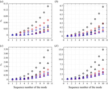
 $\varepsilon =c_{i, {BGK}-{LSE}}-c_{i, {NS}-{LSEs}}$) of the growth rate (the first ten modes) predicted by the NS-LSEs (circles denote that N–N is used, triangles denote that S–S is used) and BGK-LSE, where the horizontal coordinate axis represents the sequence number of the different modes. For the least stable mode, the deviations may be negative or positive, but in most cases, they are positive. For other modes, the values of all deviations are positive. For all cases, the deviation of the least stable modes in the first ten modes is always the smallest, but the deviation increases gradually as the Knudsen number increases, as shown in table 5, showing the relative error (
 $\delta =\varepsilon / c_{i, {B G K-L S E}}$) of the growth rate of the least stable mode. Therefore, if the NS-LSEs are used to analyse the flow with rarefaction effects, then the transition cannot be predicted accurately, and the growth rate of the least stable mode is underestimated in most cases. Comparing the deviations obtained from N–N and S–S, it can be seen that the deviation obtained from S–S is smaller than that calculated by N–N in all cases for all modes; that is, the slip boundary conditions significantly improve the stability prediction accuracy of the plane Couette flow in the slip flow regime. In addition, for a fixed
 $\alpha$, a comparison of the deviation under different Knudsen numbers indicates that the deviation increases with the Knudsen number.
Deviations ( $\varepsilon =c_{i, {BGK}-{LSE}}-c_{i, {NS}-{LSEs}}$) of the growth rate (the first ten modes) at
 $\alpha =1, 3, 6$ for (a)
 $Kn =5\times 10^{-3}$, (b)
 $Kn =1\times 10^{-2}$, (c)
 $Kn =2\times 10^{-2}$, and (d)
 $Kn =4\times 10^{-2}$. Circles denote that N–N is used, and triangles denote that S–S is used. The black line denotes
 $\alpha =1$, the red line denotes
 $\alpha =3$, and the blue line denotes
 $\alpha =6$.

The relative error ( $\delta =\varepsilon / c_{i, {B G K-L S E}}$) of the least stable mode.

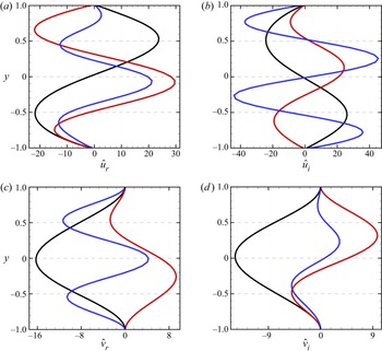
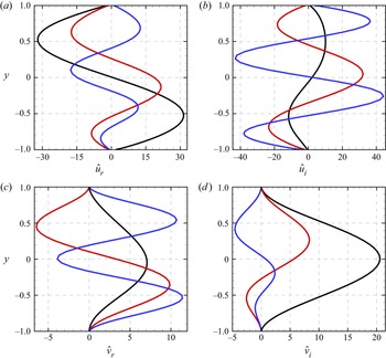
Note that under the same Knudsen number, the deviation between different modes is also different, and the deviation increases with the sequence number, as shown in figure 4. To illustrate a possible reason for this phenomenon, the imaginary and real parts of the eigenfunctions  $\hat {u}$ and
 $\hat {v}$ of the first three modes are plotted in figures 5 and 6 for
 $Kn =5\times 10^{-3}$ and
 $Kn =2\times 10^{-2}$ with
 $\alpha =1$. These figures show that the characteristic lengths of the eigenfunctions decrease with the increasing sequence number. Therefore, the Knudsen number based on the characteristic length increases with the increasing sequence number. This phenomenon is related to the Knudsen number. To further confirm this point, we plot the curves of the deviation of the least stable mode with the Knudsen number under different wavenumbers, as shown in figure 7. The variation trend of the deviation with the Knudsen number is similar to that of figure 4, which further verifies the above analysis. This also means that multiple modes constitute a multiscale problem, which needs a multiscale method to study it. As seen from figure 4, the stability analysis method in classic fluid dynamics cannot predict multiple modes accurately even when combined with Knudsen layer correction, even for flow with
 $Kn <1\times 10^{-2}$ (as shown in figure 4a). Only the mode whose characteristic scale is equivalent to the base flow characteristic scale can be predicted accurately for near-continuum flow because it is a single-scale method based on the continuum assumption. Therefore, the stability analysis method based on the NS equations should be used carefully when multiple modes are considered, such as in non-modal linear stability analysis. In addition, the failure threshold (critical
 $Kn$) of the NS-LSEs determined in § 6.2.1 is based on the base flow characteristic scale, so it does not apply to other modes; that is, the critical
 $Kn$ values within which the NS-LSEs can be used to accurately predict each mode are different, and the threshold should be determined based on the characteristic length of each mode.
Eigenfunctions of (a,b)  $\hat {u}$ and (c,d)
 $\hat {v}$ corresponding to the first three modes for the case
 ${Kn =5\times 10^{-3}}$ and
 $\alpha =1$. The black line denotes the first mode, the red line denotes the second mode, and the blue line denotes the third mode.

Eigenfunctions of (a,b)  $\hat {u}$ and (c,d)
 $\hat {v}$ corresponding to the first three modes for the case
 ${Kn =2\times 10^{-2}}$ and
 $\alpha =1$. The black line denotes the first mode, the red line denotes the second mode, and the blue line denotes the third mode.

Deviations ( $\varepsilon =c_{i, {BGK}-{LSE}}-c_{i, {NS}-{LSEs}}$) of the growth rate of the least stable mode at
 $\alpha =1, 6$ for different Knudsen numbers.

6.2.3. Effects of rarefaction on spectrum, phase speed and growth rate
The phase velocity spectra for  $Kn =1\times 10^{-4}, 5\times 10^{-3}, 1\times 10^{-2}, 2\times 10^{-2}$ and
 $\alpha =3$ are shown in figure 8. When
 $Kn =1\times 10^{-4}$, there are two more branches on the left and right branches, with
 $c_{r}=0$ as the axis of symmetry, while at larger Knudsen numbers, only one branch exists on the left and right branches, and the number of modes on these branches gradually decreases with increasing Knudsen number, and disappears when the Knudsen number is greater than a certain value. In addition, for the case
 $Kn =1\times 10^{-4}$, the eigenvalues near the junction point of the branches are very sensitive to the number of discrete nodes and will never converge. The reason for this sensitive triangle region of the spectrum is the presence of non-orthogonal eigenfunctions. In this case, a large transient growth of the energy is possible even if all eigenvalues are confined to the stable half-plane. At this time, this should be studied with the help of the non-modal stability analysis approach.
Phase velocity spectra for the plane Couette flow at  $\alpha =3$ for (a)
 $Kn =1\times 10^{-4}$, and(b)
 $Kn =5\times 10^{-3}, 1\times 10^{-2}, 2\times 10^{-2}$.

Figure 9 shows the phase velocity that corresponds to the least stable mode versus the wavenumber at different Knudsen numbers. When the phase velocity is negative, the phase velocity decreases as the Knudsen number increases, and gradually tends to  $-1$ for all Knudsen number cases. For
 $Kn =1\times 10^{-4}$, the eigenvalues all appear in pairs over the entire range of
 $\alpha$ studied. For a large Knudsen number and relatively small wavenumber, the phase velocity of the least stable mode is zero (standing wave), and with the increase in the Knudsen number, the standing wave can appear in a broader range of wavenumbers.
Phase velocity of the least stable mode as a function of the wavenumber.

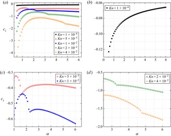
Figure 10 shows the variation in the growth rate corresponding to the least stable mode with  $\alpha$ from 0.5 to 6.0 at different Knudsen numbers. Figures 10(b–d) show magnified views of figure 10(a) for different Knudsen numbers. For a fixed
 $\alpha$, as the Knudsen number increases, if the least stable mode presents in the same pattern (travelling wave or standing wave), then the growth rate decreases; otherwise, the growth rate does not necessarily decrease. For example, from figure 9, it is seen that for the case of
 $\alpha =1.6$, when
 $Kn =5\times 10^{-3}$, the least stable mode is a travelling wave (the phase velocity is
 $-0.06619$), and when
 $Kn =1\times 10^{-2}$, the least stable mode is a standing wave (the phase velocity is
 $5.17\times 10^{-13}$). Figure 10(c) shows that when
 $Kn =5\times 10^{-3}$, the growth rate of the least stable mode is
 $-0.4433$, and when
 $Kn =1\times 10^{-2}$, the growth rate is
 $-0.4400$; that is, the growth rate at
 $Kn =1\times 10^{-2}$ is greater than that at
 $Kn =5\times 10^{-3}$.
(a) Variation in the growth rate of the least stable mode with  $\alpha$ for various Knudsen numbers.(b) Magnified view of
 $Kn =1\times 10^{-4}$. (c) Magnified view of
 $Kn =5\times 10^{-3}$ and
 $Kn =1\times 10^{-2}$.(d) Magnified view of
 $Kn =2\times 10^{-2}$ and
 $Kn =4\times 10^{-2}$.

Figure 10(b) shows that for  $Kn =1\times 10^{-4}$, the growth rate increases monotonically with the wavenumber, and the change is relatively gentle. However, for moderate to large Knudsen numbers, as figures 10(c,d) show, the variation in the growth rate with the wavenumber is non-monotonic and changes sharply at the first minimal value point, which corresponds to the wavenumber when the phase velocity changes from zero to negative, as shown in figure 9. From figure 10, for all cases except the continuum one (
 $Kn =1\times 10^{-4}$), when
 $c_{r} = 0$, the trend of change of the growth rate at different Knudsen numbers is consistent, i.e. increasing first and then decreasing; when
 $c_{r} \neq 0$, at moderate Knudsen numbers, as shown in figure 10(c), the growth rate increases and then decreases. However, at large Knudsen numbers, as shown in figure 10(d), the growth rate decreases monotonically.
Figure 11 shows the variation in the growth rate of the least stable mode with the Knudsen number for different wavenumbers ( $\alpha =0.5, 1.0, 5.5, 6.0$). Figure 9 shows that under different Knudsen numbers (
 $Kn$ from
 $5\times 10^{-3}$ to
 $4\times 10^{-2}$), for the cases
 $\alpha =0.5$ and
 $\alpha =1.0$, the least stable modes are standing waves. For the cases
 $\alpha =5.5$ and
 $\alpha =6.0$, the least stable modes are travelling waves; that is, for a fixed wavenumber, the least stable mode under different Knudsen numbers presents the same pattern (travelling or standing wave). In this case, as seen from figure 11, the growth rate decreases almost linearly with the increasing Knudsen number.
Growth rate of the least stable mode trends with the Knudsen number for different  $\alpha$.

6.2.4. Effects of rarefaction on the eigenfunctions
In this subsubsection, the effects of the Knudsen number on the eigenfunctions of the least stable mode are analysed.
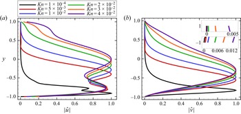
Figure 12 shows the eigenfunctions in the cases  $Kn =5\times 10^{-3}, 1\times 10^{-2}, 2\times 10^{-2}, 3\times 10^{-2}, 4\times 10^{-2}$ and
 $\alpha =1.0$. For these cases, the least stable mode is a standing wave. For different Knudsen numbers, except for the difference in the peak values of
 $\hat {u}$ at
 $y = 0.0$, the rarefaction effects have little influence on the eigenfunctions
 $\hat {u}$ and
 $\hat {v}$. While the least stable mode corresponds to a travelling wave with a negative phase velocity (
 $Kn =1\times 10^{-4}, 5\times 10^{-3}, 1\times 10^{-2}, 2\times 10^{-2}, 3\times 10^{-2}, 4\times 10^{-2}$ and
 $\alpha =6.0$), the influence of the rarefaction on the eigenfunctions is significant, as shown in figure 13. The amplitude peaks of
 $\hat {u}$ and
 $\hat {v}$ gradually shift upwards with the increasing Knudsen number. For
 $Kn =1\times 10^{-4}$, the continuum flow case, the magnitudes of
 $\hat {u}$ and
 $\hat {v}$ vanish at
 $y = 0.0$. For
 $Kn =5\times 10^{-3}$ and
 $Kn =1\times 10^{-2}$, the magnitudes of
 $\hat {u}$ and
 $\hat {v}$ vanish in the fluid domain near the upper wall. However, for a larger Knudsen number, there is still a large disturbance in the fluid domain near the upper wall. Figures 12 and 13 show that the slip velocity increases as the Knudsen number increases.
Effects of Knudsen numbers  $Kn =5\times 10^{-3}, 1\times 10^{-2}, 2\times 10^{-2}, 3\times 10^{-2}, 4\times 10^{-2}$ on the eigenfunctions (a)
 $\hat {u}$ and (b)
 $\hat {v}$ of the least stable mode for
 $\alpha =1$.

Effects of Knudsen numbers  $Kn =1\times 10^{-4}, 5\times 10^{-3}, 1\times 10^{-2}, 2\times 10^{-2}, 3\times 10^{-2}, 4\times 10^{-2}$ on the eigenfunctions (a)
 $\hat {u}$ and (b)
 $\hat {v}$ of the least stable mode for
 $\alpha =6$.

We wish to know whether the influence law of the wavenumber on the eigenfunctions is consistent in the continuum and rarefied flow regimes.
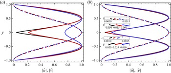
Figure 14 shows the eigenfunctions at  $Kn =5\times 10^{-3}$ and
 $2\times 10^{-2}$ under different wavenumbers
 $\alpha =0.5, 1.0, 1.5$. For these cases, the least stable mode is a standing wave. The wavenumber has little influence on the eigenfunctions
 $\hat {u}$ and
 $\hat {v}$, only causing the peak values of
 $\hat {u}$ to change at
 $y = 0.0$, and the influence law of the wavenumber on the eigenfunctions is the same in the continuum and rarefied flow regimes; that is, with the increasing wavenumber, the peak value of
 $\hat {u}$ at
 $y = 0.0$ gradually increases. Figure 14(b) shows that the slip velocity at the upper and lower walls increases as the wavenumber increases.
Effects of wavenumbers  $\alpha =0.5, 1.0, 1.5$ on the eigenfunctions
 $\hat {u}$ and
 $\hat {v}$ of the least stable mode for (a)
 $Kn =5\times 10^{-3}$ and (b)
 $Kn =2\times 10^{-2}$. The black line denotes
 $\alpha =0.5$, the red line
 $\alpha =1.0$, and the blue line
 $\alpha =1.5$. The solid and dashed lines denote
 $\hat {u}$ and
 $\hat {v}$, respectively.

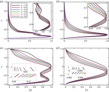
For the case of the least stable mode being the travelling wave,  $Kn =1\times 10^{-4}$ and
 $2\times 10^{-2}$ with
 $\alpha =3.5, 4.0, 5.5, 5.5, 6.0$ are considered, as shown in figure 15. As the wavenumber increases, similar to the continuum flow cases, the amplitude peaks of
 $\hat {u}$ and
 $\hat {v}$ gradually shift downwards in the rarefied flow cases. For these cases, with the increasing wavenumber, the slip velocity increases on the upper wall and decreases on the lower wall.
Effects of wavenumbers  $\alpha =3.5, 4.0, 4.5, 5.0, 5.5, 6.0$ on the eigenfunctions (a,c)
 $\hat {u}$ and (b,d)
 $\hat {v}$ of the least stable mode, for (a,b)
 $Kn =1\times 10^{-4}$ and (c,d)
 $Kn =2\times 10^{-2}$.

6.3. Non-modal stability
It is well known that if the linearized evolution operator is non-normal, then even if all eigenvalues are confined to the stable half-plane, transient energy growth can still occur. Therefore, it may be inappropriate to analyse the behaviour of a non-normal operator using its spectrum alone. In this subsection, we use the singular value decomposition method to analyse the potential for transient growth of the plane Couette flow considering the rarefaction effects.
The maximum possible amplification  $G(t)$ (Schmid & Henningson Reference Schmid and Henningson1994) of the initial perturbation energy is defined as
 \begin{equation} G(t)=\max_{q_0} \frac{E(\boldsymbol{q}(t))}{E(\boldsymbol{q}_0)}, \end{equation}
where  $E(\boldsymbol {q})$ denotes the kinetic energy of the perturbation. Under the NS analysis framework,
 $\boldsymbol {q}=(\hat {u}, \hat {v}, \hat {\rho })$. When analysing the transient energy growth based on the modal results of the BGK-LSE, the eigenfunction composed of the velocity distribution function is first converted into a macro quantity, and then the non-modal analysis is carried out using the analysis method under the NS analysis framework. For a more detailed process of calculating the transient energy growth, the reader is referred to Schmid & Henningson (Reference Schmid and Henningson1994) and Hanifi, Schmid & Henningson (Reference Hanifi, Schmid and Henningson1996).
Before we analyse the influence of the rarefaction effect on transient growth, by comparing the results based on the NS equations, the transient energy growth calculated by the BGK equation is first verified. Figure 16 shows the transient growth plots for the case  $Ma=0.1$,
 $Re=1000$,
 $\alpha =1.0$. They are in good agreement with each other.
Transient energy growth for the plane Couette flow with  $Ma=0.1$,
 $Re=1000.0$ and
 $\alpha =1.0$.

From the analysis in figure 4, we know that the NS-equations-based stability analysis method cannot predict multiple modes accurately with different characteristic lengths at the same time, while the information of multiple modes is used in the non-modal analysis, so there may be some differences between the transient energy growth based on NS and BGK equations. For this reason, the maximum transient energy growth ( $G_{max }=\max _{t>0} G(t)$) and the time (
 $t_{max }$) at which this maximum is achieved were calculated for two continuum flow cases (
 $Kn=1\times 10^{-4}, 5\times 10^{-4}$) based on the NS and BGK equations, respectively, and the relative errors of
 $G_{max }$ (
 $\delta _{G_{max }}=(G_{max , {NS}}-G_{max , {BGK}}) / G_{max , {BGK}}$) and
 $t_{max }$ (
 $\delta _{t_{max }}=(t_{max , {NS}}-t_{max , {BGK}}) / t_{max , {BGK}}$) are also analysed. The results are shown in table 6. It can be seen that the deviation is very small. However, the analysis in figure 4 does show that with the increase in sequence number, the deviation of the NS-equations-based stability analysis method in predicting growth rate increases gradually. To explain this phenomenon, we analysed the contribution of different parts of the eigenvalue spectrum to the energy growth in the case
 $Kn=5\times 10^{-4}$ and
 $\alpha =1.0$. The eigenvalue spectrum and the transient growth calculated according to different parts of the eigenvalue spectrum are given in figure 17. It can be seen that the mode with a growth rate less than a certain value has no contribution to the transient growth. Therefore, for the problems studied in the present paper, although the NS-equations-based stability analysis method cannot predict accurately multiple modes at the same time, it has little impact on transient growth in the case of continuum flow.
The maximum transient energy growth ( $G_{max }$) and the corresponding time (
 $t_{max }$) obtained from the NS and BGK equations, and the relative errors of
 $G_{max }$ (
 $\delta _{G_{max }}=(G_{max , {NS}}-G_{max , {BGK}}) / G_{max , {BGK}}$) and
 $t_{max }$ (
 $\delta _{t_{max }}=(t_{max , {NS}}-t_{max , {BGK}}) / t_{max ,{BGK}}$).

Effects of (a) different parts of the spectrum on (b) transient growth for  $Kn=5\times 10^{-4}$,
 $\alpha =1.0$. The dashed line, the solid line and the circles denote the selected portion with
 $\varpi _i>-0.6$,
 $\varpi _i>-1.5$ and
 $\varpi _i>-3.5$, respectively.

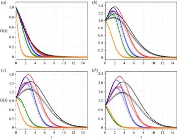
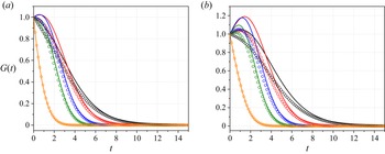
Figure 18 shows the transient energy growth at  $Kn=5\times 10^{-3}$ for different
 $Ma$ (
 $0.1, 0.2, 0.25, 0.3$) and
 $\alpha$ (
 $1.0, 1.5, 2.0, 2.5, 3.0$) values obtained by the NS and BGK equations. It can be seen that when
 $Ma$ is small, energy decays exponentially with a rate that is given by its corresponding eigenvalue. When
 $Ma$ is large, transient growth occurs in some wavenumber ranges. When the wavenumber is small, with the increase in
 $Ma$, transient growth occurs, and
 $G_{max }$ gradually increases. When
 $\alpha =2.5$, with the increase in
 $Ma$, the energy undergoes a process from exponential decay to algebraic growth and then to exponential decay. When
 $\alpha =3.0$, there is no algebraic growth in the wavenumber under consideration. In addition, by comparing the results of the NS and BGK equations, it can be seen that when transient energy growth occurs, the NS-equations-based method always overestimates
 $G_{max }$.
Transient energy growth at  $Kn=5\times 10^{-3}$ for (a)
 $Ma=0.1$, (b)
 $Ma=0.2$, (c)
 $Ma=0.25$, and (d)
 $Ma=0.3$. The lines and circles represent the results obtained by the NS equations with slip boundary conditions and the BGK equation, respectively. Black, red, blue, green and orange represent
 $\alpha =1.0$, 1.5, 2.0, 2.5 and 3.0, respectively.

Furthermore, the variation of  $G(t)$ with time at
 $Kn =0.01$ for different
 $Ma$ (
 $0.25, 0.3$) and
 $\alpha$ (
 $1.0, 1.5, 2.0, 2.5, 3.0$) values is computed, and the results are shown in figure 19. The NS-equations-based method still overestimates
 $G_{max }$. From the BGK results, we can see that when
 $Ma=0.25$, there is no transient growth. When
 $Ma=0.3$, there is a small transient growth for medium wavenumbers. In addition, by comparing
 $G_{max }$ under the same
 $Ma$ and
 $\alpha$ in figures 18 and 19, it can be seen that the higher the rarefaction degree, the smaller the
 $G_{max }$ value, and even no transient growth is possible. Therefore, we can conclude that with a higher degree of rarefaction, the transient growth may occur only in the case of a large
 $Ma$ value, and the rarefaction effect has a stabilizing effect on transient energy growth.
Transient energy growth at  $Kn={0.01}$ for (a)
 $Ma=0.25$, and (b)
 $Ma=0.3$. The lines and circles represent the results obtained by the NS equations with slip boundary conditions and the BGK equation, respectively. Black, red, blue, green and orange represent
 $\alpha =1.0$, 1.5, 2.0, 2.5 and 3.0, respectively.

7. Conclusions
We develop a novel linear stability analysis method to describe the stability of rarefied gas flows based on the BGK model equation. Different from the previous stability analysis method (Yoshida & Aoki Reference Yoshida and Aoki2006) based on kinetic theory, we solve eigenvalue problems numerically, which can solve multiple modes accurately. The validity of the novel approach is verified by the continuum flow stability results from the NS-LSEs. Furthermore, the linear stability characteristics and the non-modal transient energy growth in the plane Couette flow have been investigated using the novel approach (only the modes with  $-1< c_{r} \leq 0$ are considered). When conducting the stability analysis of rarefied flow, the method based on the NS equations with slip boundary conditions is also used. The correctness and accuracy of applying slip boundary conditions to analyse the stability of slip flow are verified. The main findings are as follows.
(1) In the near-continuum flow regime, for plane Couette flow, the NS-LSEs can accurately predict only the eigenvalues of the least stable mode for  $Kn<1\times 10^{-2}$, regardless of whether or not slip boundary conditions are used. When
 $Kn\geq 1\times 10^{-2}$, the NS-LSEs underestimate the growth rate of the least stable mode in most cases. In the slip flow regime, although the slip boundary conditions cannot capture the structure of the Knudsen layer near the wall, compared with the no-slip boundary conditions, it greatly improves the prediction accuracy of the slip flow disturbance growth rate.
(2) The characteristic length of the different modes is different, that is, the multiple mode analysis is a multiscale problem. However, the stability analysis method based on the NS equations is a single-scale method that cannot predict multiple modes accurately, even when combined with the Knudsen layer correction and even for continuum flow. Only the mode whose characteristic scale is equivalent to the base flow characteristic scale can be predicted accurately for the near-continuum flow. Therefore, the stability analysis method based on the NS equations should be used carefully when multiple modes are considered. However, for the continuum flow, the non-modal analysis shows that the error has little effect on the transient growth because the modes with small growth rates do not contribute to the transient energy growth.
(3) A change in the Knudsen number will change the pattern of the disturbance wave (standing or travelling wave). For a fixed wavenumber, only when the least stable mode presents the same pattern does the growth rate decrease almost linearly with the increasing Knudsen number. However, when the least stable mode under different Knudsen numbers appears in different patterns, the growth rate at large Knudsen numbers may be greater than that at small Knudsen numbers for some wavenumbers.
(4) When the wavenumber is small, the least stable mode is a standing wave. With the increase in the Knudsen number, the standing wave can appear in a broader range of wavenumbers. When the least stable mode is the travelling wave, with the increasing wavenumber, the growth rate increases monotonically for a small  $Kn$, first increases and then decreases for a medium
 $Kn$, and decreases monotonically for a large
 $Kn$. However, the variation law of the phase velocity with the wavenumber is not affected by the Knudsen number.
(5) For the least stable mode with a negative phase velocity, the amplitude peak of the eigenfunctions gradually moves towards the upper wall with the increase in the Knudsen number. However, the rarefaction effects have little influence on the eigenfunctions of the least stable standing mode. The influence of the wavenumber on the eigenfunctions in a rarefied flow is consistent with that in a continuum flow; that is, the amplitude peak of the eigenfunctions gradually moves towards the lower wall with the increasing wavenumber. For the least stable standing mode, the slip velocity increases with the increasing wavenumber, but for the least stable mode with a negative phase velocity, the slip velocity at the lower (upper) wall increases (decreases) with the increasing wavenumber.
(6) For the non-modal transient growth analysis, it is shown that there will still be transient growth in a rarefied flow, and the rarefaction effect plays a stabilizing role in the transient growth. The higher the  $Ma$ value, the more likely transient growth will occur in the flow with a higher rarefaction degree. For a given
 $Kn$, the trend of
 $G_{max }$ with
 $Ma$ depends on the wavenumber. When
 $\alpha$ is small,
 $G_{max }$ gradually increases with increasing
 $Ma$. In addition, when the NS-equations-based method is used to calculate the transient growth of rarefied flow, compared with the results of the BGK equation, it always overestimates the maximum transient growth.
The novel stability analysis method developed in this paper is targeted towards two-dimensional low-speed flows. For high Mach number flow, the velocity distribution function deviates from the local equilibrium state, and the temperature changes significantly. However, the Gauss–Hermite quadrature is used in our method, and the influence of temperature is not considered, so the method is limited to low-speed flow. If the newly developed stability analysis approach is used for hypersonic flow, then first, the influence of temperature needs to be considered. Additionally, the Gauss–Hermite quadrature needs to be replaced by the Newton–Cotes quadrature, but this will not affect the overall analysis framework. For three-dimensional flow, because the method developed in the present paper needs to discretize both physical space and velocity space, the computer storage and CPU requirements are far greater than those of classic stability analysis methods. For high-speed flow, the matrix dimension is more considerable. However, for three-dimensional supersonic Couette flow, there are unstable modes, and three-dimensional modes could be more unstable than their two-dimensional counterparts for some values of streamwise wavenumbers (Malik, Dey & Alam Reference Malik, Dey and Alam2008). Therefore, it is meaningful to further develop stability analysis methods suitable for high-speed three-dimensional flow and analyse the influence of the rarefaction effect on unstable modes and transient energy growth. At the same time, it is necessary to develop a matrix algorithm that can quickly solve for the eigenvalues and eigenvectors of super-large matrices. In the future, we will carry out further work in these two areas.
Acknowledgements
The authors thank X. Chen for useful discussions.
Funding
This work was supported by the National Key R&D Programme of China (2019YFA040520X), the National Numerical Wind Tunnel Project, the National Natural Science Foundation of China (nos 11902266, 11902264, 12072283), and the 111 Project of China (no. B17037).
Declaration of interests
The authors report no conflict of interest.
Data availability statement
The data that support the findings of this study are available from the corresponding author upon reasonable request.