1. Introduction
U-space facilitates the integration of drones into European airspace, leading to a surge in urban drone flights. However, the noise radiated by drones is a significant source of pollution, and hampers their widespread adoption in urban areas (Dbouk & Drikakis Reference Dbouk and Drikakis2021). Indeed, a Cherney (Reference Cherney2018), points out that drone noise is an issue for public acceptance.
The scientific community is working extensively to mitigate drone noise emissions. Consequently, this surge in research activity on isolated rotor noise has been intensified in the last few years, underscoring the current extraordinary interest in this topic. A recent review of noise control strategies has been presented by Candeloro et al. (Reference Candeloro, Martellini, Nederlof, Sinnige and Pagliaroli2022b ). However, drones are commonly multi-rotor systems. Consequently, rotor noise should be studied by considering multiple rotors to investigate the noise sources and their interplay. Indeed, the literature includes several studies focused on multi-rotor aeroacoustics. (Intaratep et al. Reference Intaratep, Alexander, Devenport, Grace and Dropkin2016; Tinney & Sirohi Reference Tinney and Sirohi2018; Dbouk & Drikakis Reference Dbouk and Drikakis2021).
In recent years, both active and passive rotor noise control techniques have been extensively studied to address this issue. Specifically, passive methods include strategies such as trailing- and leading-edge serrations on propeller blades (Turhan et al. Reference Turhan, Jawahar, Gautam, Syed, Vakil, Rezgui and Azarpeyvand2024). However, these methods can adversely affect the rotors’ aerodynamic performance, thereby diminishing their potential benefits. Consequently, recent studies have explored active noise cancellation, which reduces noise by introducing secondary sound sources, such as loudspeakers. Nevertheless, implementing this approach on multi-rotors is challenging, as it adds weight and complexity to the system (Chengyi, Yafeng & Geng Reference Chengyi, Yafeng and Geng2014).
A promising active noise control strategy for multi-rotor systems and distributed propulsion configurations, apparently free of drawbacks, involves rotor phase synchronisation. Unlike other noise mitigation strategies, this method does not require modifications to the blade shape or aerodynamic performance (Chengyi et al. Reference Chengyi, Yafeng and Geng2014). Notably, flight tests conducted on the OV-10A aircraft in 1993 demonstrated that this method could reduce cabin noise by
 $10{-}15$
dB. Furthermore, rotor synchronisation has been adopted in both military and civilian propeller aircraft (Blunt & Rebbechi Reference Blunt and Rebbechi2007). In addition, it has been successfully implemented in multi-propeller-driven unmanned aerial vehicle (Cao et al. Reference Cao, Huang, Sheng and Wang2018). The rotors of a multi-rotor aircraft act as independent noise sources; however, adjusting the relative phase angles can tune the acoustic sound field to interfere either constructively or destructively. Specifically, the phase synchronisation method leverages similar sound waves produced by the aircraft’s rotors. As a result, these waves can cancel each other out, leading to noise reduction. The main effects of synchronisation are threefold: (i) noise amplitude reduction, (ii) noise directivity modification, and (iii) noise modulation.
Indeed, several studies have reinforced the effectiveness of phase synchronisation for noise amplitude reduction. Patterson et al. (Reference Patterson, Schiller, Ackerman, Gahlawat, Gregory and Hovakimyan2020) developed a propeller phase control system that creates sound-destructive interference or generates high coherence between the two propeller sources. Consequently, this approach results in rotor noise reduction of up to
 $17$
dB at the blade passage frequency and a given observer location. Furthermore, Guan et al. (Reference Guan, Lu, Su and Xu2021) showed that phase synchronisation is highly effective for noise attenuation in quadrotors. Additionally, Hertzman, Fligelman & Stalnov (Reference Hertzman, Fligelman and Stalnov2022) underlined that phase control affects the coherent acoustic source field in a propeller system. In the same vein, Zhong et al. (Reference Zhong, Zhou, Chen, Jiang, Wu and Zhang2023) reported considerable noise reduction through phase control. In another study, Turhan et al. (Reference Turhan, Jawahar, Gautam, Syed, Vakil, Rezgui and Azarpeyvand2024) observed an approximate
 $24$
dB reduction at the first blade passage frequency, and a
 $6$
dB reduction in overall sound pressure level. Shao et al. (Reference Shao, Lu, Xu, Guan and Lu2022) concluded that phase synchronisation is more effective for co-rotating rotors than for counter-rotating ones, reducing noise by 1–5 dB and 1–11 dB, respectively.
Other studies have highlighted variations in noise directivity. Pascioni, Rizzi & Schiller (Reference Pascioni, Rizzi and Schiller2019) demonstrated that a synchrophaser can significantly alter overall noise directivity. For instance, when the rotor phase difference is
 $0^\circ$
, the rotors synchronise, resulting in a monopole directivity pattern. Conversely, for rotor phase difference
 $90^\circ$
, the directivity pattern changes to a dipole shape, with lobes rotated by
 $180^\circ$
for co-rotating rotors, and a four-leaf clover pattern for counter-rotating rotors. Moreover, Celik et al. (Reference Celik, Jamaluddin, Baskaran, Meloni, Rezgui and Azarpeyvand2024) found that the directivity patterns of the overall sound pressure level depends on the separation distance and advance ratio of the tandem propeller. Furthermore, their findings emphasised that the effectiveness of active phase control for noise reduction critically depends on precise control of both rotational speeds and blade phase angles. Finally, they hypothesised that the mechanism driving this noise reduction is attributed to destructive wave interference, a phenomenon stemming from the relative angular positioning of the propeller blades. Pandey et al. (Reference Pandey, Valdez, Beaman and Tinney2024) studied the noise produced by side-by-side synchrophased rotors, and found notable changes in the first few rotor harmonics as constructive or destructive interference occurred at different observer locations. Rotor synchronisation also has significant effects on noise modulation. Zhong et al. (Reference Zhong, Zhou, Chen, Jiang, Wu and Zhang2023) observed that random fluctuations in rotation speed led to the formation of intermittent sound wave packets. Additionally, Celik et al. (Reference Celik, Jamaluddin, Baskaran, Meloni, Rezgui and Azarpeyvand2024) highlighted that the noise emitted at the first and second blade passage frequencies is highly intermittent with amplitude modulation.
Since the interference affects the tonal component, a decomposition technique has been proposed in this paper as a first step. This technique is based on the principle that this component is coherent in space and time. Therefore, the proposed method for component separation is based on a space–time formulation of proper orthogonal decomposition. Building on this, we further investigated the interference, and developed a predictive model to determine the phase at which it occurs. An experimental validation of the model proposed is provided in the paper. Finally, a wavelet analysis was applied to the data for characterising the interference and its intermittency.
The paper is organised as follows. A description of the novel data decomposition technique is provided in § 2. Next, the experimental set-up, instrumentation and operating conditions are detailed in § 3. Then the results obtained by applying the data decomposition technique to an isolated rotor are presented in § 4.1. Subsequently, an analytical model is formulated and validated to predict the phase angles at which aeroacoustic interference occurs in §§ 4.2 and 4.3. Furthermore, the intermittent behaviour of the second harmonic is analysed through a wavelet transform in § 4.4. Finally, the conclusions are presented in § 5.
2. The space–time proper orthogonal decomposition formulation
The mathematical formulation outlined in this paper corresponds to the classical problem of space–time proper orthogonal decomposition (POD) initially proposed by Lumley (Reference Lumley1970). Although historically significant, this approach was largely overshadowed by the more widely recognised form that combines harmonic analysis methods, exercised earlier by Payne & Lumley (Reference Payne and Lumley1967) and Leib, Glauser & George (Reference Leib, Glauser and George1984) (and many other authors throughout the 1980s, 1990s and 2000s); this form was revisited by Towne, Schmidt & Colonius (Reference Towne, Schmidt and Colonius2018), where they dubbed it spectral POD. Other forms of the POD technique that have received considerable attention are the snapshot POD of Sirovich (Reference Sirovich1987) and the bi-orthogonal decomposition of Aubry (Reference Aubry1991) for space–time symmetric fields. Moreover, Schmidt & Schmid (Reference Schmidt and Schmid2019) offer a conditional space–time POD formulation aimed at constructing modes coherent in both time and space. Applications of the POD technique to problems in rotorcraft acoustics are limited, though some demonstrations can be found in the work of Tinney et al. (Reference Tinney, Zhao-Dubuc and Valdez2023, Reference Tinney, Valdez and Zhao-Dubuc2024), Bonomo et al. (Reference Bonomo, Cordioli, Colaciti, Fonseca and Simões2024) and Candeloro et al. (Reference Candeloro, Martellini, Nederlof, Sinnige and Pagliaroli2022a ).
The following mathematical formulation pertains to a one-dimensional pressure fluctuation field acquired with an array of microphones or provided by numerical simulation, but it can be extended naturally to a three-dimensional field or another variable. In this paragraph, the prime, typically used elsewhere in the paper to denote fluctuations, will be understood. A Hilbert space
 ${\mathcal{H}}$
is an inner product space that is complete in the Hilbert norm topology. We start by defining the space–time inner product over a finite time domain
 ${\mathcal{T}}$
and a finite one-dimensional space
 ${\mathcal{L}}$
:
 \begin{equation} \langle p_i, p_j\rangle =\int _{\mathcal{T}} \int _{\mathcal{L}} p_i(x,t)\,p_j^*(x,t)\,{\textrm d}x\,{\textrm d}t. \end{equation}
For clarity, we specify that in this paper, we use an asterisk superscript to denote both the complex conjugate of a scalar and the Hermitian transpose of a vector or tensor. Moreover, the domains
 ${\mathcal{T}}$
and
 ${\mathcal{L}}$
are bounded and defined as follows:
 \begin{equation} {\mathcal{T}} = \Bigl \{ t \mid t \in [0, T] \Bigr \}, \quad {\mathcal{L}} = \Bigl \{ x \mid x \in [0, L] \Bigr \}. \end{equation}
We now define a generic subdomain of
 ${\mathcal{T}}$
, namely the
 $i$
th time window, that can slide along the time axis:
 \begin{equation} {\mathcal{W}_i} = \left \{ t \mid t \in \left [ \frac {w}{2} (i-1), \frac {w}{2} (i+1) \right ] \right \}, \end{equation}
where
 $w$
is the interrogation window. Here,
 $p_i$
and
 $p_j$
represent two bounded pressure fluctuation space–time fields, defined as
 \begin{equation} p_i(x,t) = p(x,t) \ \forall t \in {\mathcal{W}_i},\forall x\in {\mathcal{L}} \quad \text{and} \quad p_j(x,t) = p(x,t) \ \forall t \in {\mathcal{W}_j}, \forall x\in {\mathcal{L}}, \end{equation}
where
 $i,j \in {\mathbb{N}}^+$
. The related norm
 $\lVert p_i \rVert$
reads
 \begin{equation} \lVert p_i \rVert = \langle p_i, p_i\rangle ^{1/2}. \end{equation}
Given the scalar product
 $\langle \cdot ,\cdot \rangle$
and an expectation operator
 $E\{\cdot \}$
, commonly defined as the ensemble average
 $\langle \cdot \rangle$
(Berkooz, Holmes & Lumley Reference Berkooz, Holmes and Lumley1993), we embed
 $p(x, t)$
into a Hilbert space
 ${\mathcal{H}}$
to identify the spatio-temporal structure
 $\phi (x, t)\in {\mathcal{H}}$
that maximises (variational approach)
 \begin{equation} \lambda =\frac {E\{ \vert \langle p,\phi \rangle \vert ^2\}}{\langle \phi , \phi \rangle }. \end{equation}
The
 $\phi (x, t)$
and
 $\lambda$
that satisfy (2.6) can be found as solutions to the Fredholm eigenvalue problem
 \begin{equation} \langle \boldsymbol{\mathcal{C}}(x,x',t,t')\,\phi (x',t')\rangle =\lambda\, \phi (x,t), \end{equation}
where
 $\boldsymbol{\mathcal{C}}(x,x',t,t')$
is the two-point space–time correlation tensor, defined as (Schmidt & Schmid Reference Schmidt and Schmid2019)
 \begin{equation} \boldsymbol{\mathcal{C}}(x,x',t,t')=E\{ p(x,t)\,p^*(x',t')\}. \end{equation}
Note that the eigenfunctions
 $\phi (x,t)$
of the space–time correlation tensor that constitutes the conditional space–time POD modes are functions of two variables, i.e. space and time. Conversely, classical and spectral POD modes are functions of only one independent variable, which is often space. Therefore, by construction, space–time POD modes are coherent in both space and time. The solution to (2.7) produces an infinite number of modes
 $(\phi _i,\lambda _i)$
, which are ranked according to their eigenvalues in descending order, such that
 $\lambda _1 \geqslant \lambda _2 \geqslant 0$
. The eigenvectors are orthogonal,
 \begin{equation} \langle \phi _i, \phi _j \rangle = \delta _{ij}, \end{equation}
and provide a complete basis for
 $p(x,t)$
. Accordingly, the space–time pressure field can be expanded as
 \begin{equation} p(x,t)=\sum ^\infty _{i=1} a_i\,\phi _i(x,t), \end{equation}
with
 \begin{equation} a_i = \langle p(x, t), \phi _i(x,t)\rangle, \end{equation}
where
 $a_i$
is the dimensionless POD coefficient.
This expansion is optimal because of its ability to capture the energy of the pressure field. Finally, the diagonal representation of the two-point correlation tensor
 $\boldsymbol{\mathcal{C}}$
insures that the modal amplitudes are uncorrelated (Berkooz et al. Reference Berkooz, Holmes and Lumley1993):
 \begin{equation} E\{ a_ia_j \}=\lambda _i\delta _{ij}. \end{equation}
2.1. Eigenvalues physical interpretation
The application of POD to problems in turbulence often alludes to it being an energy decomposition technique since the kernel comprises the turbulence stresses that make up the turbulence kinetic energy. Indeed, when the POD is applied to the fluctuating velocity field
 $\boldsymbol{V}'$
, the eigenvalues
 $\lambda _i$
represent twice the amount of fluctuating kinetic energy associated with the
 $i$
th mode (Knight & Sirovich Reference Knight and Sirovich1990; Oberleithner et al. Reference Oberleithner, Sieber, Nayeri, Paschereit, Petz, Hege, Noack and Wygnanski2011; Towne et al. Reference Towne, Schmidt and Colonius2018):
 \begin{equation} K_i=\frac {\langle \langle \boldsymbol{V}',\boldsymbol{\phi _i}\rangle ^2\rangle }{2}=\frac {\lambda _i}{2}. \end{equation}
Hence the turbulent kinetic energy can be defined as the sum of the modal contributions:
 \begin{equation} K=\tfrac {1}{2} \langle \lVert \boldsymbol{V}'\rVert ^2\rangle =\sum _{i=1}^N K_i=\tfrac {1}{2}\sum _{i=1}^N \lambda _i. \end{equation}
Certainly, there is less clarity regarding the concept of energy when POD eigenvalues are derived from pressure fields, albeit numerous applications of POD to pressure and density fields are found throughout the open literature; see, for example, Arndt, Long & Glauser (Reference Arndt, Long and Glauser1997), Tinney & Jordan (Reference Tinney and Jordan2008), Baars & Tinney (Reference Baars and Tinney2014) and Berry et al. (Reference Berry, Ali, Magstadt and Glauser2017). However, since a new definition will be useful in establishing a criterion for separating the components of the pressure signal, a simple physical interpretation has been formulated in the following.
From (2.6), it follows that the expected value of the squared pressure fluctuation associated with the
 $i$
th mode is exactly equal to the
 $i$
th eigenvalue. We build on this result using the definition of the overall sound pressure level (OASPL),
 \begin{equation} \text{OASPL}=10\log _{10}\left (\frac {\langle p^2 \rangle }{p_0^2}\right ), \end{equation}
where
 $p_0$
is the reference pressure, conventionally set to
 $20\, \mu \textrm{Pa}$
. The OASPL is a logarithmic measure of the effective sound pressure relative to a reference value. We can define the sound pressure modal level (SPML) as
 \begin{equation} \text{SPML}_i=10\log _{10}\left (\frac {\langle \langle p, \phi _i\rangle ^2\rangle }{\sum ^N_{i=1}\langle \langle p, \phi _i\rangle ^2\rangle } \frac {\langle p^2 \rangle }{p_0^2}\right )= 10\log _{10}\left (\frac {\lambda _i}{\sum ^N_{i=1}\lambda _i}\frac {\langle p^2 \rangle }{p_0^2}\right ), \end{equation}
i.e.
 \begin{equation} \text{SPML}_i=\text{OASPL}-\left | 10\log _{10}\left (\frac {\lambda _i}{\sum ^N_{i=1}\lambda _i}\right )\right |. \end{equation}
This expression quantifies the contribution of each mode to the total sound pressure level, using the eigenvalues
 $\lambda _i$
as weighting factors. Hence the
 $\text{SPML}_i$
represents the logarithmic measure of the effective sound pressure associated with the
 $i$
th mode.
It is important to emphasise that while OASPL is a point-in-time measure,
 $\text{SPML}_i$
instead provides a global characterisation of the spatio-temporal field. Moreover, it will be shown that the values of
 $\text{SPML}_i$
closely approximate those of the sound pressure spectral level (SPSL), despite being derived from spatio-temporal fields in the former case and time series in the latter. This shows that
 $\text{SPML}_i$
serves as a bridge between the Fourier space
 ${\mathcal{F}}$
and Hilbert space
 ${\mathcal{H}}$
. A similar approach, in the context of jet aeroacoustics, has previously been proposed by Tinney & Jordan (Reference Tinney and Jordan2008).
The mode expansion can be used for separating the coherent component from the stochastic one. Commonly, this result is achieved by applying an appropriate relative energy threshold:
 \begin{equation} {\mathcal{E}}_{\textit{th}}=\frac {\lambda _i}{\sum ^N_{i=1} \lambda _i}, \end{equation}
where
 ${\mathcal{E}}_{\textit{th}}$
represents the relative energy boundary between coherent and incoherent components. The energy criterion, by using the
 $\text{SPML}_i$
, becomes
 \begin{equation} \text{SPML}_{i}=\text{OASPL}-T_h. \end{equation}
In this study, the threshold was kept constant at
 $T_h=20\ \textrm{dB}$
. It will be shown that variations of this threshold around the value
 $20\ \textrm{dB}$
do not have a significant impact on the outcome. It is interesting to note that the criterion (2.19) for separating the components is a function of the OASPL. Furthermore, the variable
 $\text{SPML}_i$
is a relative value, as it represents a fraction of the total energy of the signal
 $\langle p^2 \rangle$
. Therefore, the threshold is universal for any type of signal that includes a coherent component.
2.2. A space–time POD separation technique
The aerodynamic noise of propellers can be split into two components in the Fourier domain: tonal (or narrowband) and broadband (Farassat & Succi Reference Farassat and Succi1980; Sinibaldi & Marino Reference Sinibaldi and Marino2013; Candeloro et al. Reference Candeloro, Martellini, Nederlof, Sinnige and Pagliaroli2022b ). Tonal components are directly related to the periodic motion of the blade in the surrounding fluid. Therefore, their frequencies and magnitude are related to the rotational velocity. The physical mechanism responsible for the generation of tonal contributions is associated with blade thickness and aerodynamic loading. On the other hand, broadband noise is radiated by turbulent structures or by their interaction with the blade edges (leading/trailing edge or blade tip).
Due to the distinct nature of the noise sources, tones exhibit deterministic and persistent characteristics (or global coherence), whereas the broadband counterpart exhibits random behaviour (incoherent component) (Meloni et al. Reference Meloni, de Paola, Grande, Ragni, Stoica, Di Marco and Camussi2023; Bonomo et al. Reference Bonomo, Cordioli, Colaciti, Fonseca and Simões2024). Furthermore, tonal components are coherent in both time and space, whereas the broadband component in aeroacoustics (e.g. jet, rotor and airframe noise) is incoherent in both time and space. Furthermore, the analogy can be expressed as
 \begin{equation} p' = p'_{\textit{TN}} + p'_{\textit{BB}}=p'_{c}+p'_{s}, \end{equation}
where
 $p'_{\textit{TN}}$
is the tonal component of the pressure fluctuations, and
 $p'_{\textit{BB}}$
is the broadband counterpart, whereas
 $p'_{c}$
and
 $p'_{s}$
are the coherent and stochastic (or incoherent) components, respectively.
The separation of components is essential for experimenters, as it provides valuable insights into different noise sources. Additionally, it plays a crucial role in validating simulations performed using the Ffowcs Williams–Hawkings equation. For this reason, several recent studies have focused on separating pressure fluctuations. Sree (Reference Sree2013) highlighted the difficulty of accurately distinguishing tonal and broadband noise components, particularly when two rotors operate independently without synchronisation. Meloni et al. (Reference Meloni, de Paola, Grande, Ragni, Stoica, Di Marco and Camussi2023) developed a novel wavelet-based method capable of isolating the noise emitted by a low-Reynolds-number propeller into its tonal and broadband components. Similarly, Candeloro et al. (Reference Candeloro, Martellini, Nederlof, Sinnige and Pagliaroli2022a ) proposed a separation technique based on POD application to a single time series.
Bonomo et al. (Reference Bonomo, Cordioli, Colaciti, Fonseca and Simões2024) and Malkki et al. (Reference Malkki, Yauwenas, Doolan and Moreau2024) conducted a comparative analysis of various methods available in the literature for decomposing propeller noise signals, including phase-averaging techniques. Their study found that both the wavelet transform and POD methods effectively reconstruct time series associated with both deterministic and random components. However, further research is needed to refine the separation of POD modes, as the wavelet-based approach exhibited unexpected trends (Bonomo et al. Reference Bonomo, Cordioli, Colaciti, Fonseca and Simões2024). More recently, Tinney et al. (Reference Tinney, Zhao-Dubuc and Valdez2023, Reference Tinney, Valdez and Zhao-Dubuc2024) proposed a novel method for identifying the tonal component of propeller noise. Their approach integrates POD with the Vold–Kalman order tracking filter (VKF), allowing for the isolation of signal structures in both the spatial domain (using POD) and the temporal domain (using the VKF).
Unlike the previously mentioned data-reduction methods, space–time POD does not independently decompose the spatial and temporal components of the signal. Instead, it generates modes that are mutual in both space and time. This approach is particularly well suited for problems involving a large number of time-resolved sensors, as seen in many recent experimental studies that employ microphone arrays to characterise rotor noise.
From a practical viewpoint, the proposed technique involves structuring the time series collected from microphone arrays into multiple space–time fields of limited duration. These space–time fields are then arranged as column vectors of a matrix
 $X$
, which is used to compute
 $\boldsymbol{\mathcal{C}}$
and apply the POD. As a result, the modes, eigenvalues and coefficients are computed, enabling the POD expansion, which is expressed as
 \begin{equation} p'(x,t)\approx \sum _{i=1}^N a_i\,\phi _i(x,t). \end{equation}
It is important to note that POD has been applied in a non-conventional manner: time and space separation is not performed, meaning that the modes depend on both space and time. This approach allows for the identification of space–time coherent structures. This characteristic makes the technique highly robust in separating the tonal component, ensuring coherence in both space and time.
Indeed, by properly truncating the POD expansion at the
 $j$
th mode such that
 \begin{equation} \text{SPML}_{j+1}\leqslant \text{OASPL}-20\ \text{dB}, \end{equation}
it is possible to decompose the signal into two contributions:
 \begin{equation} p'(x,t)\approx \sum _{i=1}^j a_i\,\phi _i(x,t)+\sum _{i=j+1}^N a_i\,\phi _i(x,t)=p'_{c}(x,t)+p'_{s}(x,t), \end{equation}
where
 $p'_{c}(x,t)$
represents the coherent component of the signal, and
 $p'_{s}(x,t)$
corresponds to the stochastic component.
Since this technique is based on POD, it can identify only coherence associated with dominant components, such as the sound generated by the first harmonics. However, other sources (motor, shaft) or higher-order rotor harmonics are not captured by the first modes. The advantages of using space–time POD, as well as any of the aforementioned data-reduction techniques, for problems in rotor acoustics, where signals exhibit coherence in both space and time, are as follows.
-
(i) It is simple to implement.
-
(ii) The threshold can be kept constant, and its variation has minimal impact on the results.
-
(iii) The technique is not highly sensitive to the size of the time window
 ${\mathcal{T}}$
.
-
(iv) Satisfactory results can be achieved even with a small number of microphones, in line with the configurations commonly used in aeroacoustic experiments.

3. Experimental set-up
3.1. Anechoic chamber and pressure fluctuations measurements
The investigations were conducted in the Acoustic Wind Tunnel Braunschweig (AWB), the German Aerospace Centre (DLR) small-size, high-quality anechoic test facility. This open-jet (Göttingen-type) wind tunnel is capable of operating at speeds up to
 $65\, \textrm{m}\, \textrm{s}^{-1}$
and is optimised for noise measurements at frequencies above
 $250\, \textrm{Hz}$
. The nozzle dimensions are
 $1.2\, \textrm{m}$
height and
 $0.8\, \textrm{m}$
width. During the test campaign, the wind tunnel was turned off to simulate hovering conditions.
A total of 37 microphones were used for sampling the acoustic field, arranged in four non-equidistant linear arrays. Among these, only arrays 1 and 4 are employed in the analysis presented in this paper. The microphone layout is illustrated in figure 1. The acoustic signals were sampled at
 $f_s=102\, \textrm{k}\textrm{Hz}$
using a GMB Viper GmbH 48-channel data acquisition unit for
 $30\ \text{s}$
per operating point.
Microphones layout.

3.2. Test rig description
Three-bladed propellers of type KDE-CF155-TP (
 $15.5''\times 5.3''$
) were mounted on vertical supports capable of adjusting their mutual distance (denoted as
 $d$
). The rotors have diameter
 $393.7\ \textrm{mm}$
(
 $D$
) and mean aerodynamic chord
 $28.5\, \textrm{mm}$
. The propellers were driven by KDE4012XF-400 motors and controlled by a KDEXF-UAS55 electronic speed controller. The two microphone arrays were positioned at distance
 $3.3D$
from the
 $x$
-axis, sufficiently far from the rotors to ensure that the pressure amplitudes are purely acoustic (
 $p' \propto 1/r$
).
3.3. Synchrophaser description and characterisation
A custom-made synchrophaser was implemented to control the phase delay
 $\psi (t) = \theta _2 - \theta _1$
between two co-rotating rotors operating at rotational speed
 $\omega (t)$
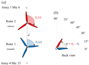
. The convention used for rotor phases and phase delay is illustrated in figure 2. The rotational speed and phase delay were measured using a Kübler 05.2400 incremental encoder with resolution 500 pulses per revolution.
(a) Graphical representation of the azimuthal rotor positions
 $\theta _1(t)$
and
 $\theta _2(t)$
; (b) relative angular position of the rotors (also referred to as phase shift or phase delay).

The synchrophaser was developed using National Instruments hardware, specifically: (i) an NI PXI-1031 chassis, (ii) an NI PXI-7350 motion controller, and (iii) an NI PXI-6259 multifunction DAQ.
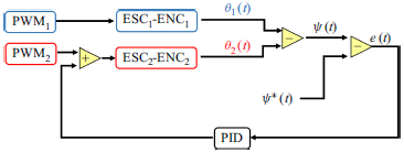
The phase shift between the rotors is controlled over time by a PID controller. It acquires the azimuthal position of both the master and slave rotors. The controller calculates the error with respect to a setpoint (
 $\psi ^*$
), and generates a pulse width modulation (PWM) control signal for the slave motor. The block diagram of the PID active control system used for propeller synchronisation is given in figure 3. Rotor 1 acted as the master, while rotor 2 operated as the slave. Considering rotor revolution time
 $11\, \textrm{ms}$
at 5200 rpm, the PID control refresh time was set to
 $5\, \textrm{ms}$
. In other words, during each half-rotation, the position of the slave rotor relative to the master was adjusted as needed.
Synchrophaser block diagram.

During the tests, the phase difference was sampled at
 $10\ \textrm{Hz}$
for
 $30\ \text{s}$
to statistically characterise the control system’s performance. Figure 4 presents the mean and standard deviation of the phase difference between the propellers at various rotational speeds for a phase setpoint of zero (
 $\psi ^*=0$
). The standard deviation of the phase difference is represented as an error bar overlaid on all markers. The typical standard deviation of the instantaneous phase relative to the setpoint was found to be less than
 $1.2^\circ$
at 5200 rpm. The synchroniser demonstrated highly satisfactory performance, as evidenced by the stable rotational speeds and consistent relative phase differences between the propellers during characterisation.
Mean phase delay values at different rotational speeds, with phase shift setpoint zero. Error bars indicate the standard deviation of the phase delay.

3.4. Test matrix
The experiments were conducted with the wind tunnel deactivated to simulate hovering conditions. The phase difference between the propellers was varied systematically in increments of
 $15^\circ$
. Three different centre-to-centre distances between the rotor hubs were tested:
 $d/D = 1.02$
,
 $d/D = 1.10$
and
 $d/D = 1.20$
. The rotational speed of the rotors was kept constant at 5200 rpm, equivalent to 86.66 rps.
In total, 22 different test cases were analysed, including a reference test with an isolated rotor for comparative purposes. The detailed test matrix is provided in table 1.The test conditions correspond to blade tip Mach number
 $M_{\textit{tip}}=\omega R/c_\infty =0.31$
and Reynolds number
 $Re_{c75}=1.51\times 10^5$
. The Reynolds number at
 $75\, \%$
of the propeller radius is calculated as
 \begin{equation} Re_{c75}=\frac {0.75\omega\, R c_{75} }{\nu }, \end{equation}
where
 $\omega$
is the rotational speed in
 $\text{rad s}^{-1}$
,
 $c_{75}$
is the chord calculated at
 $75\, \%$
of the propeller radius, and
 $\nu$
is the kinematic viscosity of the air, assumed to be
 $1.51\times 10^{-5}\ \textrm{m}^2\ \textrm{s}^{-1}$
.
Test matrix. Test case no. 0 refers to an isolated rotor.

4. Results
4.1. Space–time POD of the pressure fluctuation
The pressure fluctuations, denoted as
 $p'$
, sampled by a linear array of microphones, are plotted in a dimensionless space–time domain. Time and space are normalised using the blade passing frequency
 $f^*$
and the corresponding wavelength
 $\lambda ^*=c/f^*$
, where
 $c$
is the speed of sound at temperature
 $293.15\,\textrm K$
. The pressure fluctuations generated by an isolated rotor are shown in figure 5 over a dimensionless time interval equivalent to four times the period of a blade passage. The figure reveals a distinct pattern consisting of four alternating curved black-and-white streaks, corresponding to expansion fronts followed by compression waves. In the spatial sub-domains
 $x/\lambda ^*\lt 0$
and
 $x/\lambda ^*\gt 1$
, a reduction in wavefront intensity is observed due to the directivity of tonal noise and the increasing distance between the microphones and the source. The wavefronts are perfectly equispaced in time, an effect associated with the stability of the active control system regulating the rotational speed. Additionally, the field appears to be highly noisy, with irregular horizontal streaks that characterise the stochastic component of the sound.
Pressure fluctuations generated by the isolated rotor with the wind tunnel turned off (
 $U_\infty =0\, \textrm{m}\, \textrm{s}^{-1}$
). Dimensionless representation of the pressure fluctuations in space and time, as recorded by microphone array 4. The red-and-white circles indicate the positions of the microphones along the
 $x$
-axis.

By applying a windowing process to the acquired time series, 1020 fields were generated, from which the correlation tensor
 $\boldsymbol{\mathcal{C}}(x,x',t,t')$
was constructed. The size of the correlation tensor
 $\boldsymbol{\mathcal{C}}$
is
 $1020 \times 1020$
, and its rank is 1020. This indicates that the tensor is of full rank, meaning that all its modes contribute to the data representation. The eigenvalues, modes and coefficients were then computed.
(a) Spectrum of eigenvalues for an isolated rotor obtained by analysing microphone array 4. (b) The SPML on modal order
 $n$
. The dashed blue line represents
 $\text{OASPL}-20\ \textrm{dB}$
, while the blue dash-dotted line represents the value assumed by the OASPL.

In figure 6(a), the obtained eigenvalue spectrum is shown on a logarithmic scale. The first six dominant modes have relative energy greater than
 $1\, \%$
. These eigenvalues appear in pairs with similar values, suggesting a coupling between modes. In addition, figure 6(b) provides the same information as in figure 6(a) in terms of identifying coupled and dominant modes. However, figure 6(b) also provides additional information that is particularly valuable in acoustics and aeroacoustics, namely the amount of noise associated with each mode, measured in decibels (dB). This information in dB complements the relative energy information, offering a more comprehensive view of the modal dynamics and their acoustic implications. In figure 6(b), a blue band represents the new criterion for selecting coherent modes. It is noteworthy that all the coherent modes selected, following a conventional criterion, fall within this coherence band. The comparison between
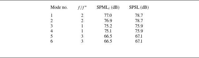
 $\text{SPML}_i$
and the conventional SPSL is reported in table 2 . It is observed that the SPSL consistently appears higher than
 $\text{SMPL}_i$
. This discrepancy is explained by the fact that the SPSL is computed by using microphone 33, located closer to the noise source and on the rotor plane, where pressure fluctuations are higher. In contrast,
 $\text{SPML}_i$
represents the measurement of the entire microphone array.
Comparison between the values assumed by
 $\text{SPML}_i$
and SPLS for the first six modes.

Figure 7 shows the first six space-time modes that turn out to be very similar pairwise. Degenerate modes occur when two or more eigenvalues coincide. The most prevalent type of degeneracy is termed double modes, as in this case, where only two eigenvalues are identical. According to Hasan & Sanghi (Reference Hasan and Sanghi2007), the translational symmetry in both space and time of these degenerate modes confirms the presence of travelling waves. Moreover, all three pairs exhibit directivity effects.
First six modes for an isolated propeller calculated using time history acquired by linear array of microphones 4.

Figure 8 shows the auto-power spectrum of the modes at a specific position
 $x/\lambda \approx 0.5$
(i.e. at microphone 33). The results indicate that the modes are perfectly harmonic over time. In particular, the modes are characterised by regular oscillations at distinct frequencies: (i) modes 1–2,
 $f/f^* = 2$
; (ii) modes 3–4,
 $f/f^* = 1$
; (iii) modes 5–6,
 $f/f^* = 3$
. The POD has effectively selected the Fourier basis as its kernel. As noted by Lumley (Reference Lumley1981) and Tinney & Jordan (Reference Tinney and Jordan2008), POD simplifies to harmonic orthogonal decomposition when the analysed field is homogeneous, periodic, or stationary in a given direction. This latest result confirms that the inequality
 $\text{SPML} \lt \text{SPSL}$
is related to directivity. Indeed, the signal energy outside the rotor plane reduces SPML, which accounts for this effect. In contrast, SPSL is computed only on the rotor plane and remains higher.
Power spectrum of the first three modes calculated at specific position
 $x/\lambda \approx 0.5$
(i.e. for microphone 33) and reported in dimensionless form.

Phase portraits of the first six POD coefficients.

Lissajous patterns are observed in the phase portraits of the POD coefficients
 $a_i$
and
 $a_j$
, as shown in figure 9. The shapes of the Lissajous curves are determined by the amplitude, frequency and phase of the two series of values. Observing them allows for the assessment of the frequency ratio between
 $a_i$
and
 $a_j$
(Oberleithner et al. Reference Oberleithner, Sieber, Nayeri, Paschereit, Petz, Hege, Noack and Wygnanski2011). Some useful information for interpreting the phase portraits is provided in Appendix A. In figure 9(a,b,c), circular patterns are observed, indicating a phase difference
 $\pi /2$
between the coefficients, and the same frequency. Conversely, in figure 9(d), an eight-like pattern is observed, corresponding to frequency ratio
 $f_i/f_j = 2$
and phase difference
 $\pi /2$
. Furthermore, in figure 9(e), an
 $\alpha$
-shaped pattern is observed, indicating frequency ratio
 $f_i/f_j = 2/3$
and phase difference
 $\pi /2$
. Finally, in figure 9(f), the curve exhibits a candy-like shape, which corresponds to frequency ratio
 $f_i/f_j = 1/3$
and phase difference
 $\pi /2$
. This result aligns with the nature of the phenomenon, as pure travelling waves will have orthogonal components of the same magnitude (Feeny Reference Feeny2008). The presence of these Lissajous curves indicates that the first six modes are regular waves propagating over time.
Representation of the input–output of the separation technique: (a,d) the raw data, (b,e) the tonal component, and (c,f) the broadband component, for (a,b,c) the space–time fields, and (d,e,f) a single time series extracted at
 $x/\lambda ^* = 0.45$
, located in the rotor plane.

4.1.1. Pressure fluctuation separation
By applying the data decomposition technique to the raw data
 $p'(x/\lambda ^*,tf^*)$
shown in figure 10(a), the pressure fields were separated into the tonal component
 $p_{c}(x/\lambda ^*,tf^*)$
, depicted in figure 10(b), and the broadband component
 $p'_{s}(x/\lambda ^*,tf^*)$
, shown in figure 10(c). Figure 10(d,e,f) show the results of the decomposition for a single time series extracted at
 $x/\lambda ^* = 0.45$
, located in the rotor plane. The signal in figure 10(e) is much smoother, and perfectly in phase with the raw signal.
Furthermore, the separation technique was computed with
 $T_h=20\,\text{dB}$
and interrogation window
 $w=4/f^*$
. These values were selected by performing a sensitivity analysis. More specifically, figure 11 displays how the coherent component varies with the threshold. In particular, for threshold values
 $T_h\lt 17\,\text{dB}$
, there is a loss of signal energy, whereas for
 $T_h\gt 23\,\text{dB}$
, the stochastic component of the signal becomes noticeable. Therefore, threshold
 $T_h=20\,\text{dB}$
was selected, representing an intermediate value within the
 $[17,23]\ \text{dB}$
interval and corresponding to
 $\lambda _i/\sum \lambda _i=0.01$
.
Pressure fluctuation associated with the coherent component calculated for different values of
 $T_h$
.

According to Pierce (Reference Pierce1981) and Mancinelli et al. (Reference Mancinelli, Pagliaroli, Di Marco, Camussi and Castelain2017), the SPSL of the data is computed as
 \begin{equation} \textit{SPSL}=10\log _{10}\frac {\textit{PSD}\,\Delta f_{0}}{p_{0}^2}, \end{equation}
where PSD stands for power spectral density, and
 $\Delta f_{0}=5\,\textrm{Hz}$
and
 $p_{0}=20\, \mu \rm{Pa}$
are, respectively, the frequency resolution and the reference pressure.
In figure 12, the spectrum of the raw signal is compared with those of the coherent and incoherent components. Furthermore, the frequencies are represented in a dimensionless form by normalising them with the blade passage frequency (
 $f^*$
). In this figure, the coherent component,
 $p'_c$
, exhibits an almost flat trend over the range
 $f/f^*\in [0.1,\, 1)$
. Furthermore, the first three harmonics of this component match those of the raw signal. Conversely, beyond the third harmonic, the spectrum gradually decays. Moreover, minor peaks present between the first three harmonics in the raw signal’s spectrum are cancelled by the separation technique. This characteristic is particularly intriguing, as it significantly distinguishes the technique from a standard band-pass filter. Notably, the spectrum of the coherent component exhibits its highest peak at the second harmonic rather than the first. This behaviour is attributed to the installation effect, which amplifies the second harmonic. Such a phenomenon aligns with findings reported in the literature (Whelchel, Alexander & Intaratep Reference Whelchel, Alexander and Intaratep2020; Zarri et al. Reference Zarri, Dell’Erba, Munters and Schram2022).
Commonly, the installation effect refers to the influence of surrounding structures (e.g. wings, fuselage, or ground surfaces) on the generation and propagation of aerodynamic noise. These structures can reflect, scatter or amplify acoustic waves, causing constructive or destructive interference that modifies the perceived noise intensity. In this study, the term installation effect specifically denotes pylon–rotor interaction noise.
The SPSL calculated at
 $x/\lambda ^*=0.45$
for the raw data, tonal and broadband components.

In figure 13, the probability density function (PDF) of the incoherent signal follows a Gaussian distribution up to
 $3\sigma$
, suggesting that this component can be considered stochastic (Mancinelli et al. Reference Mancinelli, Pagliaroli, Di Marco, Camussi and Castelain2017). However, beyond
 $3\sigma$
, a departure from the standard Gaussian distribution is evident, with the PDF tails exceeding those of the reference Gaussian distribution. This discrepancy in the tails is commonly attributed to intermittent pressure events (Mancinelli et al. Reference Mancinelli, Pagliaroli, Di Marco, Camussi and Castelain2017; Pagliaroli et al. Reference Pagliaroli, Mancinelli, Troiani, Iemma and Camussi2018; Candeloro, Ragni & Pagliaroli Reference Candeloro, Ragni and Pagliaroli2024).
By contrast, the PDF of the coherent component exhibits a quadri-modal shape with four peaks of similar probability. The outer peaks, located at
 $p'/\langle p'^2 \rangle ^{1/2} \approx \pm 2$
, represent the main signature generated by the blade passage. The inner peaks are linked to additional fluctuations caused by installation effects, which increase the second harmonic in the spectrum. Each blade passage produces a pair of strong positive and negative peaks, followed by a weaker secondary pair. In conclusion, the Gaussian shape of the PDFs for the incoherent component and the quadri-modal shape for the coherent component indicate that the proposed decomposition technique is effective in separating the
 $p_c'$
and
 $p_s'$
components.
The PDFs of the tonal and stochastic components of the pressure fluctuation.

4.2. Interference function: one-dimensional formulation
The overall tonal aeroacoustic field produced by two rotors is obtained by summing their individual, non-interacting sound fields. According to Tam, Salikuddin & Hanson (Reference Tam, Salikuddin and Hanson1988), rotor noise fields with the same number of blades and angular frequency either cancel or reinforce each other. This effect, known as acoustic interference, depends on the relative phase at the observation point, and determines whether the resulting interaction leads to constructive or destructive interference. A mathematical model for predicting acoustic interference between rotors is highly valuable and can be utilised to minimise tonal noise. For engineering applications, such a model can support the design of quieter distributed electric propulsion systems or even be integrated into active noise control systems.
An analytical model, hereafter referred to as the interference function, is introduced in this paper to predict the acoustic interference between propellers. For modelling purposes, the rotors are assumed to have the same number of blades, rotate with the same angular frequency, and maintain a constant phase shift. The mathematical formulation is carried out in a coordinate reference frame located at the midpoint between the propellers, as illustrated in figure 14(a).
(a) Sketch of the two rotors labelled for identification, with corresponding angular positions and a half-distance between them. It includes reference microphones and a reference frame. (b) Pressure fluctuations generated by the passage of the propellers, specifically sampled by microphone 6. (c) Similarly, pressure fluctuations sampled by microphone 33. Time delays are depicted, taking into account both distance and phase delays, with their respective signs. The time location
 $t_0$
serves as a reference point used to define all delays.

Moreover, the mathematical formulation of the interference function is based on three characteristic time delays: (i) distance half time delay
 $\tau _d$
; (ii) phase time delay
 $\tau _\psi$
; (iii) coherent noise (or tonal) half time scale
 $\tau _{c}$
.
These time delays depend on the separation distance between the rotors, the rotational regime and the observer’s position.
More specifically, the half time delay due to the separation distance between rotors can be defined as
 \begin{equation} \tau _d=\frac {d}{2c}, \end{equation}
while the time delay resulting from the phase shift between rotors is investigated by Dobrzynski (Reference Dobrzynski1993) and Tinney & Valdez (Reference Tinney and Valdez2020), and can be defined as
 \begin{equation} \tau _\psi =\frac {\psi B}{2\pi f^*}, \end{equation}
where
 $B$
is the number of blades. Finally, the half time scale of the signature associated with the blade passage is defined as
 \begin{equation} \tau _c:\,\rho _{\textit{pp}}(\tau _c)\leqslant \rho _{\textit{pp}}(\tau )\quad \forall \tau \in [0, +\infty ), \end{equation}
where
 $\rho _{\textit{pp}}(\tau _c)$
represents the absolute minimum of the autocorrelation coefficient of
 $p'(t)$
.
Although the model can be extended easily to predict the phenomenon at a generic point in space, the following formulation is limited to a sub-domain along the
 $z$
-axis defined as
 \begin{equation} \mathcal{Z} = \left\{(y,z) \in \mathbb{R}^2 \mid y=0 \text{ and } z \in \left(-\infty , -\frac {d+D}{2}\right] \cup \left[\frac {d+D}{2}, +\infty \right)\right\}, \end{equation}
where the tonal component reaches maximum intensity.
In the interference function formulation, time delays must be considered with the appropriate signs. To this aim, figure 14 depicts two scenarios, illustrating the effects of time delays at microphones 6 and 33, both positioned on the rotor plane. Regarding microphone 6, as shown in figure 14(b), an increase in separation distance or phase shift leads to a greater delay between the signatures produced by the corresponding blades of the two rotors. In contrast, for microphone 33, an increase in phase shift leads to a reduction in the delay between the red and blue signals, as illustrated in figure 14(c). The function
 $\text{sgn}(z)$
takes into account the sign of
 $\tau _\psi$
, and it is defined as
 \begin{equation} \text{sgn}(z) = \left \{ \begin{array}{rl} 1, & \text{if } z \gt 0, \\ 0, & \text{if } z = 0, \\ -1, & \text{if } z \lt 0, \end{array} \right . \end{equation}
with
 $n\in \mathbb{N}$
.
The mathematical model is based on the fundamental principle that constructive interference occurs when the sum of the delays is zero or an integer multiple of the blade pass period, i.e.
 \begin{equation} \tau =2\tau _d+\text{sgn}(z)\,\tau _\psi =\frac {n}{f^*}. \end{equation}
By substituting the expressions for
 $\tau _d$
and
 $\tau _\psi$
into (4.7), we obtain
 \begin{equation} \frac {d}{c}+\text{sgn}(z)\,\frac {\psi B}{2\pi f^*}=\frac {n}{f^*}. \end{equation}
In practical applications, only two cases are relevant:
 $n=0$
and
 $n=1$
. For
 $n=0$
, the pressure fluctuations generated by the corresponding blades of the two rotors are perfectly synchronised. For
 $n=1$
, the fluctuation generated by the
 $i$
th blade of one rotor is synchronous with the pressure fluctuation generated by the
 $(i-1)$
th blade of the other rotor.
Consequently, starting from (4.8), it is possible to define the interference function as
 \begin{equation} \mathcal{I}_n(d,\psi ,f^*,B)= \left\{ \begin{array}{c@{\quad}l} \text{sgn}(z)\,\dfrac {d2\pi f^*}{c\psi B}, & \text{if } n=0,\\[8pt] \dfrac {df^*}{c}+\text{sgn}(z)\,\dfrac {\psi B}{2\pi }, & \text{if } n=1. \end{array} \right. \end{equation}
The interference function
 $\mathcal{I}_n$
depends on the rotational regime, number of blades, phase shift and separation distance between the rotors. When
 $\mathcal{I}_n$
assumes the unitary value, constructive interference occurs.
Two scenarios are described below to provide an example of the mathematical tool’s application. With reference to the scenario depicted in figure 14(c), for
 $n=0$
and
 $z\lt 0$
, the condition for constructive interference is given by
 \begin{equation} \mathcal{I}_0(d,\psi ,f^*,B)=\frac {d2\pi f^*}{c\psi B}=1. \end{equation}
Physically, this means that the signature generated by blade 2 of rotor 2 overlaps in time and space with that generated by the corresponding blade of rotor 1. The second scenario proposed corresponds to constructive interference for
 $n=1$
and
 $z\gt 0$
(see figure 14
b). In this case, a wavefront emitted by blade 2 of rotor 2 coincides with that generated by the preceding blade of rotor 1 (blade 1). The condition governing this scenario can be expressed as
 \begin{equation} \mathcal{I}_1(d,\psi ,f^*,B)=\frac {df^*}{c}+\frac {\psi B}{2\pi }=1. \end{equation}
Starting from the acoustic synchronisation conditions of the two rotors, (4.7), it is possible to define the phase opposition condition using
 $\tau _c$
:
 \begin{equation} \tau =2\tau _d+\text{sgn}(z)\,\tau _\psi =\frac {n}{f^*}\pm \tau _c. \end{equation}
Thus destructive interference occurs when
 \begin{equation} \mathcal{I}_1(d,\psi ,f^*,B)=1\pm \tau _c f^* \end{equation}
or
 \begin{equation} \mathcal{I}_0(d,\psi ,f^*,B)=-\text{sgn}(z)\pm \frac {\tau _c 2\pi f^*}{\psi B}. \end{equation}
In figure 15(a,b), the black dashed quarter-circle of radius 1 indicates the constructive interference condition, and the black solid lines denote destructive conditions. The blue, red and green curves depict interference functions at three distances for
 $n=0$
and
 $n=1$
. In figure 15(a),
 $\mathcal{I}_1$
is computed for the three distances
 $d/D = 1.02$
,
 $1.10$
and
 $1.20$
, which were also tested experimentally. The interference functions intersect only two interference conditions: one corresponding to destructive interference, and the other to constructive interference. Moreover, the phase shifts at which these intersections occur depend on the distance between the rotors. In figure 15(b),
 $\mathcal{I}_0$
is displayed for the same three distances. Three intersections with the black curves are observed, indicating that by varying the phase between
 $0^\circ$
and
 $90^\circ$
, two conditions of destructive interference and one condition of constructive interference can be achieved.
Plot of the destructive interference conditions (black solid lines), constructive interference condition (black dashed line), and interference functions for
 $d/D=1.02$
(blue solid line),
 $d/D=1.10$
(red dash-dotted line), and
 $d/D=1.20$
(green dashed line). Here,
 $\mathcal{I}_n$
is computed for (a)
 $n=1$
,
 $z\gt 0$
, and (b)
 $n=0$
,
 $z\lt 0$
.

4.3. Comparison between experimental results and interference function
The pressure fluctuation time histories from microphones 6 and 33 were decomposed into tonal and broadband components, as described in § 2.2, to focus the analysis solely on the coherent signal. This decomposition is applied specifically because the interference phenomenon pertains exclusively to the tonal component. Subsequently, the
 $\text{OASPL}_c$
, the SPSL for the first and second harmonics, and the autocorrelation at
 $\tau =1/2f^*$
were computed and are presented in figures 16 and 17. These figures depict the relationship between the previously listed acoustic quantities, the phase difference, and the distance ratio
 $d/D$
. They also include dashed black circles, representing the isolated rotor values, as a reference.
The
 $\text{OASPL}_c$
, SPSL and autocorrelation coefficient as functions of phase shift calculated from the time histories sampled by microphone 6, for (a,b,c,d)
 $d/D=1.02$
, (e,f,g,h)
 $d/D=1.10$
, and (i,j,k,l)
 $d/D=1.20$
.

In figure 16(a,e,i), the
 $\text{OASPL}_c$
is shown as a function of
 $\psi$
, calculated for three different distances. The first observation is that the
 $\text{OASPL}_c$
associated with the tandem rotor is generally higher than that of the isolated rotor. For
 $d/D = 1.02$
, the maximum
 $\text{OASPL}_c$
occurs at
 $\psi _M = 90^\circ$
(constructive interference), while two minima are visible at
 $\psi _m=0^\circ$
and
 $\psi _m=60^\circ$
, corresponding to destructive interference conditions. As the rotor distance increases from
 $d/D = 1.02$
to
 $d/D = 1.20$
, the maximum shifts to
 $\psi _M = 75^\circ$
. More generally, the entire curve shifts by
 $\Delta \psi = -15^\circ$
as the distance between the rotors increases (see figure 16
a,i).
The OASPL, SPSL and autocorrelation coefficient as functions of phase shift, calculated from the time histories sampled by microphone 33, for (a,b,c,d)
 $d/D=1.02$
, (e,f,g,h)
 $d/D=1.10$
, and (i,j,k,l)
 $d/D=1.20$
.

This effect influences both the first and second harmonics, as is evident from the comparison between figures 16(b,f,j) and 16(c,g,k). While the impact of distance and phase is noticeable for both harmonics, it is particularly pronounced for the second harmonic. The presence of the second rotor significantly alters the dynamic system, with the signal’s energy and its dependence on phase and distance being more pronounced in the second harmonic. The signal closely resembles that emitted by a single rotor with six blades. Therefore, to better investigate this phenomenon, it is useful to define a new frequency as an alternative to the conventional blade pass frequency
 $\hat {f}=f^*N$
, where
 $N$
is the number of rotor.
Finally, in figure 16(d,h,l), the correlation coefficient at
 $\tau =1/2f^*$
shows the same trend as
 $\text{SPSL}_2$
, as expected. Specifically, for the phase angles where destructive interference occurs, the autocorrelation coefficient tends towards −1. Since this parameter is constantly bounded between 1 and −1, with −1 representing the condition of maximum noise mitigation, it could be used as the objective function in an active noise-cancellation control system.
Figure 17 displays a single constructive interference at
 $\psi _M=45^\circ$
, and two destructive interferences at
 $\psi _m=15^\circ, 75^\circ$
. The effect of varying the rotor’s separation distance is not visible, which is related to the time delay signs depicted in figure 14. This is a particularly interesting finding, as it indicates a lack of symmetry in the directivity of tandem rotor noise, in contrast to the behaviour observed with an isolated rotor. At this position, stronger effects of destructive interference are observed, reducing the sound level below that of the isolated rotor. This outcome highlights the potential of noise cancellation techniques for multi-rotor noise mitigation by appropriately selecting the phase shift and separation distance between propulsion systems.
Figure 18 compares the phase delays at which interference occurs, as detected experimentally, with those predicted using the interference function proposed in § 4.2. For the experimental data, a vertical error bar, corresponding to the discretisation step of the phase shift, represents the uncertainty in identifying the interference condition. Additionally, for destructive interference only, a horizontal error bar of
 $\varepsilon _\psi = 240f^*/f_s$
has been introduced to account for the uncertainty in determining the time scale of the signature associated with the blade passage.
Comparison between experimentally measured phase delays corresponding to the occurrence of the interference phenomenon and those predicted by the interference function.

Although the experimental phase discretisation is relatively coarse, resulting in a significant margin of uncertainty in identifying interference conditions, the comparison between the data points and the bisector of the first and third quadrants demonstrates a satisfactory agreement between the experimental results and the formulated mathematical model.
4.4. Noise intermittency
The phenomenon of intermittency and the chaotic behaviour of pressure fluctuations has been systematically addressed within the context of thermoacoustic instability (Kabiraj & Sujith Reference Kabiraj and Sujith2012; Kashinath, Li & Juniper Reference Kashinath, Li and Juniper2018; Guan, Gupta & Li Reference Guan, Gupta and Li2020) through the use of time–frequency representations and recurrence quantification analysis. However, there are no studies that thoroughly investigate the phenomenon of rotor noise intermittency. Intermittency is one of the common routes to chaos and occurs when a dynamical system switches between irregularly spaced alternating intervals of chaotic/burst and steady/periodic states (Klimaszewska & Żebrowski Reference Klimaszewska and Żebrowski2009; Pagliaroli & Troiani Reference Pagliaroli and Troiani2020). In fluid dynamics, the term intermittency was introduced to describe signals that alternate between flat and bursting behaviour, interpreted, respectively, as laminar and turbulent states (Platt, Spiegel & Tresser Reference Platt, Spiegel and Tresser1993).
The current literature provides several criteria for the classification of intermittency. One of the most common classification systems is introduced by Bergé et al. (Reference Bergé, Dubois, Mannevillel and Pomeau1980) and Pomeau & Manneville (Reference Pomeau and Manneville1980), who categorise intermittency into three classes associated with a different bifurcation scenario: (i) type I, intermittency related to a saddle-node bifurcation; (ii) type II, intermittency due to a Hopf bifurcation, identified by the appearance of a quasi-periodic state; (iii) type III, intermittency related to a reverse period doubling bifurcation.
The following analysis focuses on four specific operating conditions, using microphone 33 (
 $z\lt 0$
) and rotor distance ratio
 $d/D=1.20$
:
-
(i)
$\psi _m=15^\circ$
, destructive interference; -
(ii)
$\psi _i=60^\circ$
, transition between constructive and destructive interference; -
(iii)
$\psi _M=45^\circ$
, constructive interference.


In these three conditions, the nature of the signal changes completely; in particular, for one specific condition, the signal becomes strongly time-dependent. The time–frequency analysis of the noise enables a qualitative investigation of the time-dependent nature of the pressure fluctuations that is crucial for identifying transient or intermittent phenomena in propeller aeroacoustics.
This study employs the continuous wavelet transform to analyse localised time–frequency fluctuations in microphone signals. Similar to the Fourier transform, the energy density can be derived from wavelet coefficients as shown in Tinney & Sirohi (Reference Tinney and Sirohi2018):
 \begin{equation} E(s,\tau )=\frac {\vert w(s,\tau )\vert ^2}{\Delta s}, \end{equation}
where
 $w(s,\tau )$
are the wavelet coefficients. Finally, sound pressure wavelet level (SPWL) can be calculated as
 \begin{equation} \text{SPWL}(f,\tau )=20\log _{10}\frac {\vert w(f,\tau )\vert }{p_0}. \end{equation}
In particular, the present analysis was performed by selecting a complex Morlet wavelet, which is a solution of the wave equation (Visser Reference Visser2003) and fits the nature of the problem. For interested readers, further details on the wavelet transform can be found in Pagliaroli et al. (Reference Pagliaroli, Pagliaro, Patane, Tatí and Peng2020).
In figure 19 , the space–time pressure fluctuation field, the tonal component of the time series, and its wavelet transform in the normalised time–frequency domain are computed and presented for the three different conditions.
(a,d,g) Pressure fluctuations represented in the space–time domain. (b,e,h) Time histories sampled by microphone 33. (c,f,i) The SPWL in the time–frequency domain. (a,b,c) Destructive interference (
 $\psi _m=15^\circ$
). (d,e,f) The transition condition between constructive and destructive interference (
 $\psi _i=60^\circ$
). (g,h,i) Constructive interference (
 $\psi _M=45^\circ$
).

In figure 19(b), only one dominant oscillation per blade passage period is observed, with a significantly smaller amplitude compared to the other cases (see figure 19 e,h). Destructive interference occurs, leading to substantial noise cancellation. For this condition, figure 19(c) shows that the signal energy is primarily concentrated in the first harmonic, as expected, although its intensity remains low. The second harmonic is completely cancelled. This reduction in energy at the second harmonic, associated with destructive interference, was recently observed and explained by Del Duchetto et al. (Reference Del Duchetto, Pagliaroli, Candeloro, Rossignol and Yin2025).
In figure 19(d–f), an intermediate case between constructive and destructive interference is observed. The energy associated with the second harmonic becomes intermittent, exhibiting amplitude modulation and forming irregular wave packets. This phenomenon has also been reported by Tinney & Sirohi (Reference Tinney and Sirohi2018), Zhong et al. (Reference Zhong, Zhou, Chen, Jiang, Wu and Zhang2023) and Celik et al. (Reference Celik, Jamaluddin, Baskaran, Meloni, Rezgui and Azarpeyvand2024). In this circumstance, the phenomenon becomes chaotic, and the observed intermittency in the second harmonic is of type II. In figure 19(i), the intermittency of the second harmonic fully transitions into periodic dominant radiation.
Zhong et al. (Reference Zhong, Zhou, Chen, Jiang, Wu and Zhang2023) associate the intermittency of sound with fluctuations in rotational speed. The results indicate that intermittency is linked to proximity to constructive interference conditions, where small variations produce significant effects. This local emergence or disappearance of a periodic oscillation is characteristic of subcritical Hopf bifurcations. The influence of proximity to constructive interference has not been emphasised previously, yet we believe that it is crucial for understanding this recently studied phenomenon. A deviation from destructive interference conditions leads to modulation of the tonal component, which, in turn, enhances the perception of annoyance (Celik et al. Reference Celik, Jamaluddin, Baskaran, Meloni, Rezgui and Azarpeyvand2024).
5. Conclusions
This paper examines noise generation by side-by-side co-rotating propellers for different phase shifts and separation distances, focusing on the rotor’s aeroacoustic interference. Additionally, aeroacoustic installation effects have been addressed.
A technique for separating tonal and broadband noise components, based on the space–time coherence of pressure waves, is formulated and discussed. Within this mathematical framework, a sound pressure modal level has been defined, providing valuable insight into the entire spatio-temporal pressure field in terms of effective acoustic pressure. This metric is used to establish a component separation criterion.
Furthermore, a mathematical model referred to as the interference function has been formulated. This model is based on the time delay introduced by the phase shift and rotor separation distance. The interference function predicts the phase delays at which different types of interference occur at a given location, rotational regime and blade number. The model has been validated experimentally, showing excellent agreement with the experimental data. These results can inform the development of active noise control systems and the design of quieter distributed propulsion systems. In future work, this model will be generalised to predict interference phenomena across the entire far field.
Furthermore, it has been observed that destructive interference primarily affects the second harmonic, and the autocorrelation value has been identified as a useful indicator of noise cancellation. Specifically, destructive interference cancels the second harmonic and weakens the first, while constructive interference amplifies both harmonics. Additionally, for phase shift values close to constructive interference, an intermittent and aperiodic phenomenon has been observed. This suggests a transition to chaos via subcritical Hopf bifurcations. This aspect is currently being further investigated using advanced chaotic analysis techniques.
Acknowledgements
We are indebted to the anonymous referees whose valuable comments have contributed to the improvement of the quality of this paper. Research activities described in the paper are part of the work carried out by the GARTEUR AG-26 consortium, which has promoted the collaboration between the German Aerospace Center (DLR) and University Niccolò Cusano.
Declaration of interests
The authors report no conflict of interest.
Author contributions
T.P.: conceptualisation, methodology, software development, formal analysis, investigation, writing original draft, writing review & editing, visualisation. P.C.: data acquisition, writing review & editing, visualisation. F.D.D.: conceptualisation, data acquisition, data pre-processing, experimental design. K.-S.R.: conceptualisation, methodology, software development, data acquisition, investigation. J.Y.: conceptualisation, supervision, project administration, funding acquisition, investigation.
Appendix A. Lissajous curves
Lissajous or Bowditch curves emerge as the superposition of a horizontal with a vertical harmonic motion. They are named after the french physicist Jules Antoine Lissajous, who studied them intensively. Lissajous patterns are shapes related to the amplitude, frequency, phase and distortion/clipping of the two series
 $x = \sin (\omega _x t)$
and
 $y = \sin (\omega _y t + \theta )$
. By observing them, it is also possible to evaluate the frequency ratio
 $f_r = \omega _x/\omega _y$
, as sketched in figure 20.
Lissajous curves.