2.1. Problem definition

First, we extend Moore's solution for the evolution of a spatially periodic vortex sheet with a family of initial perturbations. Evolution of the vortex sheet in two-dimensional potential flow is described by a parameterized complex curve

(2.1)\begin{equation} z(\varGamma,t) = x(\varGamma,t)+{\rm i}y(\varGamma,t), \end{equation}

where $t$ is time and $\varGamma$ measures the circulation in the sheet between an arbitrary point with coordinate $z$ and a reference fluid particle chosen as $\varGamma =0$. The sheet shape evolution in time is governed by the BR equation

(2.2)\begin{equation} \frac{\partial {\bar{z}}(\varGamma,t)}{\partial t}=\frac{1}{2{\rm \pi} {\rm i}}{\int\hskip -1,05em -\,}_{-\infty}^{\infty}\frac{{\rm d}\hat{\varGamma}}{z(\varGamma,t)-z(\hat{\varGamma},t)}, \end{equation}

where ${\bar {z}}$ is the complex conjugate of $z$ and the right-hand side is understood as a Cauchy principal-value (CPV) integral. We will assume that $z(\varGamma,t)$ satisfies two conditions

(2.3)\begin{equation} z(\varGamma+2{\rm \pi},t) = 2{\rm \pi} + z(\varGamma,t),\quad z(-\varGamma,t) ={-}z (\varGamma,t). \end{equation}

Using the second condition, (2.2) can be written in the form

(2.4)\begin{equation} \frac{\partial {\bar{z}}(\varGamma,t)}{\partial t}=\frac{1}{2{\rm \pi} {\rm i}}{\int\hskip -1,05em -\,}_0^{\infty}\left(\frac{1}{z(\varGamma,t)-z(\hat{\varGamma},t)} +\frac{1}{z(\varGamma,t)+z(\hat{\varGamma},t)}\right)\,{\rm d}\hat{\varGamma}. \end{equation}

We consider an initial-value problem that uses a general initial sinusoidal perturbation of the form

(2.5)\begin{equation} z(\varGamma,0)=\varGamma+ {\rm e}^{{\rm i}\phi} \epsilon \sin(\varGamma), \end{equation}

with initial amplitude $0<\epsilon \ll 1$ and phase $\phi \in [0,2{\rm \pi} )$. The real component $\epsilon \cos \phi$ stretches the circulation distribution while the imaginary component $\epsilon \sin \phi$ perturbs the sheet shape. Moore (Reference Moore1979) studied the particular case where $\phi ={\rm \pi} /2$. See Krasny (Reference Krasny1986b), Cowley et al. (Reference Cowley, Baker and Tanveer1999) and Shelley (Reference Shelley1992) for discussion of and results for alternative initial conditions. The unperturbed sheet with $\epsilon =0$ corresponds to the uniform shear flow with velocity field given by

(2.6)\begin{equation} \boldsymbol{u}(x,y)=\left\{ \begin{array}{@{}ll@{}} \displaystyle\left(-\frac{1}{2},0\right), & y>0,\\ \displaystyle\left(\frac{1}{2},0\right), & y<0. \end{array} \right. \end{equation}

2.2. Fourier expansion

For $t>0$, Moore (Reference Moore1979) expresses the sheet function in a Fourier series

(2.7)\begin{equation} z(\varGamma,t)=\varGamma+\sum_{n={-}\infty}^{\infty}\mathcal{A}_n(t) {\rm e}^{{\rm i}n\varGamma}, \end{equation}

here with initial conditions according to (2.5)

(2.8)\begin{equation} \mathcal{A}_{{\pm} 1}(0)={\mp} \frac{{\rm i}\,{\rm e}^{{\rm i}\phi} \epsilon}{2},\quad \mathcal{A}_n(0)=0,\quad (n\neq{\pm} 1). \end{equation}

It immediately follows from symmetry that

(2.9)\begin{equation} \mathcal{A}_0(t)=0,\quad \mathcal{A}_{{-}n}(t)={-}\mathcal{A}_n(t). \end{equation}

Substituting (2.7) into (2.2) leads to a system of ordinary differential equations (ODEs) for the Fourier coefficients $\mathcal {A}_n$

(2.10)\begin{equation} \frac{{\rm d}\bar{\mathcal{A}}_{{-}n}}{{\rm d}t}=\frac{{\rm i}}{2{\rm \pi}}\left[\mathcal{A}_nI_1+\sum_{r_1+r_2=n}\mathcal{A}_{r_1}\mathcal{A}_{r_2}I_2+\cdots+ \sum_{r_1+r_2+\cdots+r_K=n}\left(\prod_{p=1}^{K}\mathcal{A}_{r_p} I_K\right)+\cdots\right], \end{equation}

where $I_K$ is the principal-value integral with respect to $\xi =\hat {\varGamma }-\varGamma$

(2.11)\begin{equation} I_K={\int\hskip -1,05em -\,}_\infty^\infty \prod_{p=1}^K(1-{\rm e}^{{\rm i}r_p \xi})\xi^{{-}K-1}\,{\rm d}\xi, \end{equation}

where $r_p=1,2,3,\ldots$ are indices of $\mathcal {A}$, and $p=1,2,3,\ldots$ are sub-indices for $r$.

To estimate $\mathcal {A}_n$, the system of (2.10) can be further partitioned by the power series expansion

(2.12)\begin{equation} \mathcal{A}_n(t)=\sum_{j=0}^\infty \epsilon^{|n+2j|}\mathcal{A}_{n,{2j}}(t), \end{equation}

giving subsystems of ODEs for each $\mathcal {A}_{n,0}$, $\mathcal {A}_{n,2}$, $\mathcal {A}_{n,4}$,…. In particular, at leading order, $O(\epsilon ^{|n|})$, the corresponding integral defined in (2.11) can be calculated using residues as

(2.13)\begin{equation} I_K={\rm \pi} {{\rm i}^{K+1}} ({-}1)^{K} \prod_{p=1}^Kr_p,\quad (r_p\geq 1), \end{equation}

leading to the following evolution equations for $\mathcal {A}_{n,0}$:

(2.14)\begin{align} \frac{{\rm d}\bar{\mathcal{A}}_{n,0}}{{\rm d}t}=\frac{1}{2}\left[\!\mathcal{A}_{n,0}(-{\rm i})n+\cdots+\left(\!\sum_{\substack{r_1+r_2+\cdots+r_K=n\\r_1,r_2,\ldots,r_K\geq 1}}(-{\rm i})^K\prod_{p=1}^K \mathcal{A}_{r_{p},0}\,r_p\!\right)+\cdots+\mathcal{A}_{1,0}^n(-{\rm i})^n\!\right]\!. \end{align}

The first two equations read explicitly as

(2.15a,b)\begin{equation} \frac{{\rm d}\bar{\mathcal{A}}_{1,0}}{{\rm d}t}={-}\frac{{\rm i}}{2}\mathcal{A}_{1,0},\quad \frac{{\rm d}\bar{\mathcal{A}}_{2,0}}{{\rm d}t}={-}{\rm i}\mathcal{A}_{2,0}-\frac{1}{2}\mathcal{A}_{1,0}^2. \end{equation}

2.2.1. Asymptotic coefficients

The ODE system (2.14) and (2.8) can be solved recursively to give, for example, the asymptotic ${\mathcal {A}}_{1,0}$ and ${\mathcal {A}}_{2,0}$ for large $t$ as follows:

(2.16)\begin{equation} \left. \begin{gathered} \mathcal{A}_{1,0}=\frac{(1+{\rm i}){\rm e}^{t/2}}{4}\lambda_{1,0}+O({\rm e}^{{-}t/2}),\\ \mathcal{A}_{2,0}=\frac{(1+{\rm i}){\rm e}^{t}}{16}(\lambda_{2,0}\,t+\lambda_{2,1})+O({\rm e}^{{-}t}), \end{gathered} \right\} \end{equation}

where

(2.17)\begin{equation} \left. \begin{gathered} \lambda_{1,0} \equiv \lambda_1= \sin\phi-\cos\phi,\\ \lambda_{2,0}=\frac{\lambda_1^2}{2}=\frac{1-\sin 2\phi}{2},\quad\lambda_{2,1}=\frac{4 \cos 2 \phi -\sin 2 \phi -1+(1-\sin 2 \phi ){\rm i}}{4}. \end{gathered} \right\} \end{equation}

Here, we require $\lambda _1\neq 0$, i.e. $\phi \neq {\rm \pi}/4, 5{\rm \pi} /4$, to retain the leading-order behaviour. Special cases with $\lambda _1=0$ are not considered in this study.

Moore (Reference Moore1979) showed by induction that the solution for the leading-order $\mathcal {A}_{n,0}$ takes the form

(2.18)\begin{equation} \mathcal{A}_{n,0}\sim \frac{(1+{\rm i}){\rm e}^{nt/2} }{4^n}[\lambda_{n,0}t^{n-1}+\lambda_{n,1}t^{n-2}+\cdots], \end{equation}

where, by abbreviating $\lambda _{n} \equiv \lambda _{n,0}$, the leading-order coefficient $\lambda _n$ for $n\geq 2$ is given by the following recursion:

(2.19)\begin{equation} \lambda_n=\frac{1}{2(n-1)}[(n-1)\lambda_1 \lambda_{n-1}+2(n-2)\lambda_2\lambda_{n-2}+\cdots+(n-1)\lambda_{n-1}\lambda_1]. \end{equation}

To determine the large $n$ behaviour of $\lambda _n$, Moore (Reference Moore1979) proposed a generating function $g(x)$ defined for $x\in \mathbb {R}$ as

(2.20)\begin{equation} g(x)=\sum_{n\geq 1} \lambda_n x^n, \end{equation}

with

(2.21)\begin{equation} g'(0) = \lambda_1, \end{equation}

given by (2.17). The recursion (2.19) thus implies

(2.22)\begin{equation} g'(x) = \frac{1-\sqrt{1-2g(x)}}{x}. \end{equation}

Equations (2.22) and (2.21) can be solved in closed form as

(2.23)\begin{equation} g(x)={-}\tfrac{1}{2} W_0(-\lambda_1 x) \left[W_0(-\lambda_1 x)+2\right], \end{equation}

where $W_0$ is the Lambert W function. Taylor expanding (2.23) around $x=0$ yields

(2.24)\begin{equation} g(x)=\sum_{n\geq 1}c_n\lambda_1^n x^n =\lambda_1 x+\frac{\lambda_1^2 x^2}{2}+\frac{\lambda_1^3 x^3}{2}+\frac{2\lambda_1^4 x^4}{3}+\cdots.\end{equation}

Therefore, comparing (2.20) and (2.24) shows

(2.25)\begin{equation} \lambda_n =c_n \lambda_1^n. \end{equation}

Here, $c_n>0$ given in (2.24) also corresponds to the special case $\lambda _1=1$ (i.e. $\phi ={\rm \pi} /2$) studied by Moore (Reference Moore1979), where it is shown that

(2.26)\begin{equation} c_n\sim \frac{e^n}{\sqrt{2{\rm \pi}}n^{5/2}}, \end{equation}

as $n\to \infty$. Finally, substituting (2.26), (2.25) and (2.18) into (2.12) completes the following asymptotic Fourier coefficients $\mathcal {A}_n$ for $t\gg 1$, $n\gg 1$ and $t\gg n$:

(2.27)\begin{equation} \mathcal{A}_n(t)\sim \frac{(1+{\rm i})[\text{sign}(\lambda_1)]^n}{\sqrt{2{\rm \pi}}n^{5/2} t}\exp\left\{n\left[1+\frac{t}{2}+\ln \left(\frac{|\lambda_1|\epsilon t}{4}\right)\right]\right\}. \end{equation}

Compared with the special case of $\lambda _1=1$, it is seen that a general $\lambda _1\neq 0$ simply rescales the initial perturbation size $\epsilon$ to $|\lambda _1|\epsilon$ for the coefficients $|\mathcal {A}_n(t)|$.

2.2.2. Critical time of singularity formation

Owing to correction terms contained in (2.18), the leading-order $\mathcal {A}_{n,0}$ given by (2.27), as an approximation of $\mathcal {A}_{n}$, deteriorates in accuracy as $n\to \infty$ for fixed $t$. Moore (Reference Moore1979) resolved this non-uniformity by introducing a strained time $s$, and consequently obtained

(2.28)\begin{align} \mathcal{A}_{n,0}(t)=\frac{1}{\sqrt{2{\rm \pi}}}n^{-({5}/{2})}\left(\frac{\lambda_{1}}{4}s {\rm e}^{{s}/{2}+1}\right)^n\left[\frac{1+{\rm i}}{s}+O\left(\frac{1}{s^2}\right)\right],\quad s=t+\frac{\alpha_1}{t}+O(t^{{-}2}), \end{align}

where $\lambda _{1}=1$ and $\alpha _1=2$. In Appendix A, we show that (2.28) also holds for the general case of $\lambda _{1}\neq 1$, where the constant $\alpha _1=\alpha _1(\phi )$ as a function of $\phi$ is given by (A13).

Equations (2.12) and (2.28) imply that, in contrast to (2.27), the uniformly convergent Fourier coefficients are expressed in terms of $s$ as follows:

(2.29)\begin{equation} \mathcal{A}_n(t(s))\sim \frac{(1+{\rm i})[\text{sign}(\lambda_1)]^n}{\sqrt{2{\rm \pi}}n^{5/2} s}\exp\left\{n\left[1+\frac{s}{2}+\ln \left(\frac{|\lambda_1|\epsilon s}{4}\right)\right]\right\}. \end{equation}

Therefore, at a critical time $t_c(\epsilon )$ defined by

(2.30)\begin{equation} 1+\frac{s_c}{2}+\ln s_c=\ln\left(\frac{4}{|\lambda_1|\epsilon}\right), \quad t_c=s_c+O(s_c^{{-}1}), \end{equation}

the $\mathcal {A}_n$ values for the Fourier series (2.7) given by (2.29) lose their exponential decay for $t\ge t_c$, and transition to algebraic decay as $O(n^{-5/2})$. Consequently, the initially smooth vortex sheet spontaneously loses analyticity of its shape function $z$ at $t_c$, when a singularity develops. This singularity is of the same form as that exhibited in (2.27), but occurs at a slightly different time. For small perturbation size $\epsilon$, and consequently large critical time, $t_c$ can be well approximated by solving (2.30) at leading order to give

(2.31)\begin{equation} t_c=2W_0\left(\frac{2}{e|\lambda_1 |\epsilon}\right), \end{equation}

where $W_0$ is again the Lambert W function.

2.3. Sheet structure at critical time

Using (2.7), (2.8) and (2.12), the series describing the vortex-sheet shape can be asymptotically summed for small $\epsilon$ as

(2.32)\begin{equation} z(\varGamma,t)=\varGamma+2{\rm i}\sum_{n=1}^\infty \mathcal{A}_n(t) \sin(n\varGamma)\simeq \varGamma+2{\rm i}\sum_{n=1}^\infty \mathcal{A}_{n,0}(t)\epsilon^n \sin(n\varGamma). \end{equation}

With $\mathcal {A}_{n,0}$ given by (2.28), the Fourier series (2.32) converges uniformly to

(2.33)\begin{gather} z(\varGamma,t) \simeq \varGamma-\frac{\begin{array}{l}\left(1+{\rm i}\right) \left[\text{Li}_{{5}/{2}}\left(\frac{\text{sign}(\lambda_1)t|\lambda_1|\epsilon}{4} {\rm e}^{-{\rm i} \varGamma+1+({t}/{2})}\right) -\text{Li}_{{5}/{2}}\left(\frac{\text{sign}(\lambda_1)t|\lambda_1|\epsilon}{4} {\rm e}^{{\rm i} \varGamma+1+({t}/{2})}\right)\right]\end{array}}{\sqrt{2 {\rm \pi}} t}, \end{gather}

for all $t\leq t_c$ up to the critical time $t_c$ given by (2.31), where $\textrm {Li}_n(s)\equiv \sum _{p=1}^\infty s^p/p^n$ is the polylogarithm function. Evaluating (2.33) at $t=t_c$ yields the critical sheet shape, ${z_c=z(\varGamma,t_c)}$, as follows:

(2.34)\begin{equation} z_c(\varGamma) \simeq \varGamma-\frac{\left(1+{\rm i}\right) \left[\text{Li}_{{5}/{2}}\left(\text{sign}(\lambda_1) {\rm e}^{-{\rm i} \varGamma}\right)-\text{Li}_{{5}/{2}}\left(\text{sign}(\lambda_1) {\rm e}^{{\rm i} \varGamma}\right)\right]}{\sqrt{2 {\rm \pi}} t_c}. \end{equation}

Equation (2.28) is valid for $n$ large, and the addition of low-mode corrections would modify (2.34). This is expected to be analytic and so will not change the nature of the singularity.

If $\lambda _1>0$ then, near the origin, where $0 \le \varGamma \ll 1$, (2.34) takes the asymptotic form

(2.35)\begin{equation} z_c({\varGamma}) \sim b(\varGamma+A \varGamma^{3/2} )+O(\varGamma^2), \end{equation}

where

(2.36a,b) \begin{align} b(\lambda_1\epsilon) = 1 - \frac{(1-{\rm i})\,\zeta\left(\frac{3}{2} \right)} {\sqrt{2{\rm \pi}}\,W_0\left( \frac{2}{{\rm e}\,\lambda_1\epsilon} \right)} ,\quad A(\lambda_1\epsilon) = \frac{1} {\frac{3}{4}\, (1+{\rm i})\,W_0\left(\frac{2}{ {\rm e}\,\lambda_1\epsilon} \right) - \frac{3\zeta\left( \frac{3}{2} \right) }{2\,\sqrt{2{\rm \pi}}}} , \end{align}

and $\zeta (3/2)\approx 2.61238$ is a constant following the Riemann zeta function $\zeta ({\cdot })$. Both (2.33) and (2.34) satisfy $z(-\varGamma,\tau ) = -z(\varGamma,\tau )$ as required but (2.35) does not because the complex constants are tailored to $\varGamma \ge 0^+$. This will not affect the subsequent analysis. An expression for the sheet shape at $t=t_c$, $\varGamma <0$ which satisfies the proper symmetry can be obtained but is not needed. Equation (2.35) agrees with a similar result at $t=t_c$ obtained by Cowley et al. (Reference Cowley, Baker and Tanveer1999), although estimates of constants differ.

Similarly, if $\lambda _1<0$, (2.34) can be expanded around $\varGamma ={\rm \pi}$ to show the same power series as (2.35). Since the role of $\lambda _1\neq 1$ in both cases is to rescale $\epsilon$ while preserving the same sheet shape near the singularity, we subsequently commit to the Moore (Reference Moore1979) initial value with $\lambda _1=1$, i.e. $\phi ={\rm \pi} /2$, without loss of generality. The variation of both the real and imaginary parts of $b(\epsilon )$ and $A(\epsilon )$ ($\lambda _1=1$) are displayed in figure 1. For $\epsilon \le 0.0439064$, the argument of $A$ lies in the fourth quadrant, crossing to the third quadrant for larger values. Later the special case $\mathrm {Re}[A]=\mathrm {Im}[A]$ or $\arg [A] = 5{\rm \pi} /4$ will arise. This occurs with $\epsilon = 0.248985,A = -0.639680 - 0.639680\textrm {i}, b=i$ which is nominally out of range of the present discussion. Calculations will generally use $\epsilon = 10^{-3}$ for which $b = 0.791266 + 0.208734\textrm {i}$, $A = 0.116149 - 0.199386\textrm {i}$. Asymptotic results with $\epsilon \to 0$ will also be presented.

Figure 1.

(a) Real (solid) and imaginary (dashed) parts of $b(\epsilon )$ vs $\epsilon$. (b) Real (solid) and negative imaginary (dashed) parts of $A(\epsilon )$ vs $\epsilon$.

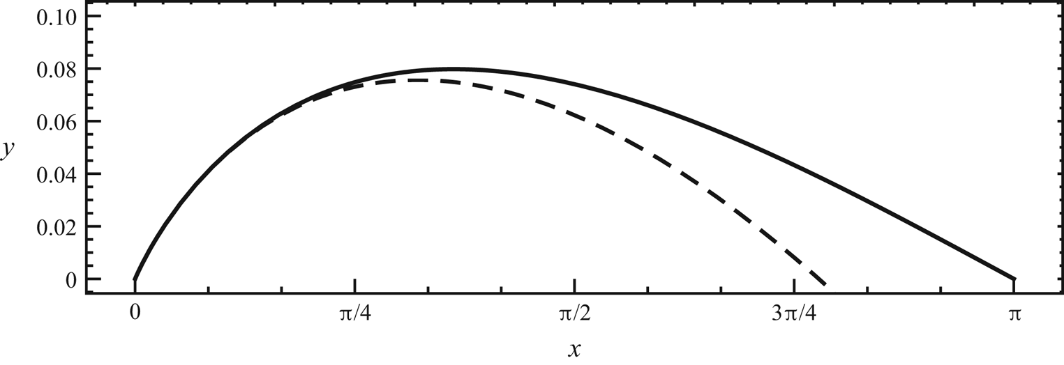
Figure 2 shows the sheet shape in $0\le x \le {\rm \pi}$ for $\epsilon = 10^{-3}$ given by both (2.34) and the leading-order approximation (2.35). With $\epsilon = 10^{-3}$, the sheet angle at the origin at $t=t_c$ is $\arg [b(10^{-3})] = 0.257922$ radians or $14.7779^\circ$. The vortex-sheet strength, $\gamma \equiv |\partial z/\partial \varGamma |^{-1}$, which measures the jump in tangential velocity across the sheet, can be calculated from (2.34) at $t=t_c$ as

(2.37)\begin{equation} \gamma_c= \left| \frac{(1+{\rm i}) \sqrt{{\rm \pi} } {t_c}}{(1+{\rm i}) \sqrt{{\rm \pi} } {t_c}-\sqrt{2} [\text{Li}_{{3}/{2}}({\rm e}^{-{\rm i} \varGamma})+\text{Li}_{{3}/{2}} ({\rm e}^{{\rm i} \varGamma})]}\right|,\end{equation}

which is continuous for all $\varGamma \in [0,2{\rm \pi} ]$. From (2.37) or using (2.35)–(2.36a,b) it can be shown that, with $t=t_c$, as $\epsilon$ increases and $A$ crosses the imaginary axis at $\epsilon = 0.0439064$, then $\gamma _c$ changes from a local maximum, with negative singular gradient at $\varGamma \to 0^+$, to a local minimum while the sheet angle at the singular point passes through $\arg [b] = 45^\circ$. Since $\epsilon <<1$ for the Moore solution we will generally consider $\mathrm {Re}[A]>0$.

Figure 2.

Vortex-sheet geometry at $t=t_c$. Here, $\epsilon = 10^{-3}$. Solid black: (2.34). Dashed: first two terms on the right-hand side of (2.35).

Using (2.35), the sheet curvature $\kappa$ for small $\varGamma$ follows as

(2.38)\begin{equation} \kappa\sim \frac{t_c^2}{\left(2 \alpha ^2-2 \alpha t_c+t_c^2\right){}^{3/2} \sqrt{\varGamma}}=O\left(\frac{1}{\sqrt{\varGamma}}\right), \end{equation}

with $\alpha =\sqrt {2/{\rm \pi} }\zeta (3/2)\approx 2.084$, which is singular when $\varGamma \to 0^+$.

2.4. Continued solution beyond critical time

We now address the motion of the sheet near $\varGamma \to 0$ for small times after $t_c$, $t>t_c$ where $\tau \equiv t-t_c\ll 1$. This is first explored by analytically continuing the Fourier series solution for the sheet shape $z$ obtained in (2.32) and (2.33) outside its domain of uniform convergence. Indeed, for $t< t_c$, the polylogarithm function $\textrm {Li}_{{5}/{2}}(w)$ contained in the summed form (2.33) with varying $\varGamma \in [0,2{\rm \pi} ]$ is evaluated inside the complex unit disk $\{w\in \mathbb {C},\,|w|<1\}$, where $\textrm {Li}_{{5}/{2}}({\cdot })$ remains a holomorphic function of $\varGamma$. When $t=t_c$, $\textrm {Li}_{{5}/{2}}({\cdot })$ is accessed along the unit circle, and its branch point $w=1$ is approached from both sides as $\varGamma \to 0$ in (2.33). As a result, the critical sheet shape $z_c$ loses analyticity at $\varGamma =0$, but remains continuous. For $t > t_c$, i.e. $\tau >0$, the asymptotic Fourier coefficients $\mathcal {A}_{n,0}$ given in (2.28) diverge as $n\to \infty$, and therefore the series solution breaks down. The summed form (2.33), originally obtained for $t < t_c$ can nonetheless be evaluated when $t>t_c$ as an analytic continuation because $\textrm {Li}_{{5}/{2}}(w)$ is in fact holomorphic for all $w\in \mathbb {C}\backslash (1,\infty )$. With $\lambda =1$ and $t= t_c+\tau$, this gives

(2.39) \begin{equation} z_{AC}(\varGamma,\tau) = z(\varGamma,t_c+\tau) \simeq \varGamma-\frac{\left(1+{\rm i}\right) [\text{Li}_{{5}/{2}}(J {\rm e}^{-{\rm i} \varGamma})-\text{Li}_{{5}/{2}}(J {\rm e}^{{\rm i} \varGamma})]}{\sqrt{2 {\rm \pi}} \left[2 W_0\left(\frac{2}{e \epsilon }\right)+\tau\right]}, \end{equation}

where (2.31) is used, and

(2.40)\begin{equation} J=J(\tau)= {\rm e}^{\tau /2} \left(\frac{\tau }{2W_0\left(\frac{2}{e \epsilon }\right)}+1\right). \end{equation}

At the origin $z_{AC}(\varGamma \to 0^+,0)=0$ but since $J>1$ when $\tau >0$ the branch cut discontinuity along $w\in (1,\infty )$ of $\textrm {Li}_{{5}/{2}}(w)$ is crossed as $\varGamma \to 0^+$ in (2.39), leading to a discontinuous jump of the vortex-sheet profile at the origin. Specifically, this discontinuity at $\tau =0^+$ is given by $z_{AC}(0^+,0)=0$ when $\tau =0$ and

(2.41) \begin{equation} z_{AC}(0^+,\tau)=\lim_{\varGamma\to 0^+}\left[ z_{AC}(\varGamma,\tau)\right]=\frac{\sqrt{2}(1-{\rm i})\mathrm{Im}[\text{Li}_{{5}/{2}}(J(\tau))]}{\sqrt{\rm \pi}\left[2 W_0\left(\frac{2}{e \epsilon }\right)+\tau\right]}, \end{equation}

when $\tau >0$. Immediately after the critical time $t_c$, (2.41) is expanded for $\tau \ll 1$ as

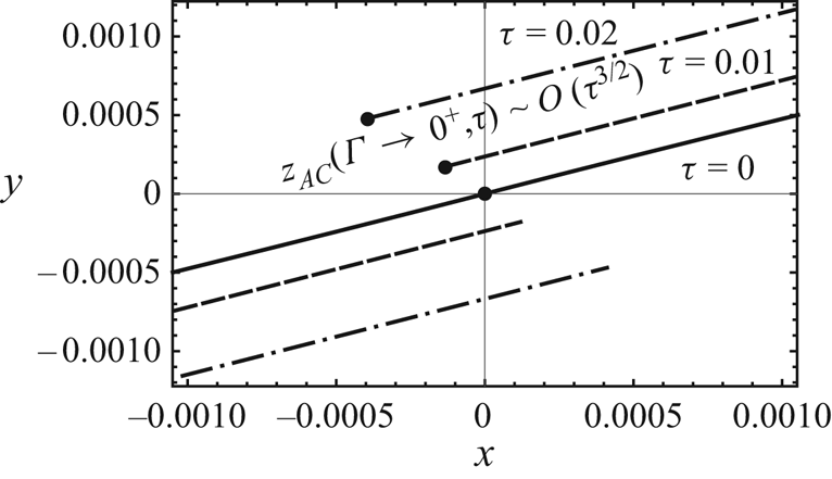
(2.42)\begin{equation} z_{AC}(0^+,\tau)\sim \frac{({-}1+{\rm i})\left(\frac{1}{W_0\left(\frac{2}{e \epsilon }\right)}+1\right)^{3/2} \tau ^{3/2}}{3W_0\left(\frac{2}{e \epsilon }\right)}+O(\tau^2), \end{equation}

suggesting that, when $\tau > 0$, the vortex sheet, which passes through the coordinate origin at $\tau = 0$, separates into two distinct branches (sheet tearing) whose ends or tips separate as $\tau ^ {3/2}$. This is shown in figure 3, where the analytically continued sheet shape is shown near the origin for two values of $\tau$.

Figure 3.

Vortex-sheet geometry near endpoints given by the analytic continuation (2.39), with ${\tau = 0,0.01,0.02}$ and $\epsilon =0.01$. Endpoint positions with $\varGamma \to 0^+$ shown as large dots for the right-hand sheet branch as given by (2.42).

In the following we put $b = |b|\exp (\textrm {i}\,\theta )$, $A = |A|\exp (\textrm {i}\,\chi )$, where $|b|$, $|A|$, $\theta$ and $\chi$ are known functions of $\epsilon$. We will refer interchangeably to variable sets $(\varGamma,\tau )$ and $(\eta,\tau )$ where

(2.43)\begin{equation} \tau = t - t_c,\quad \tau\ll1,\quad \eta = \frac{\varGamma\,|b|^2}{\tau}. \end{equation}

For clarity, we will refer to three regions defined for now by

1. (i) $\textrm {I}\quad \textrm {Outer:} \quad \eta \gg 1,\quad 2{\rm \pi} >\varGamma >0,\quad \varGamma \gg \tau$;

2. (ii) $\textrm {II}\quad \textrm {Intermediate:}\quad \eta = {O}(1),\quad \varGamma = {O}(\tau )$;

3. (iii) $\textrm {III}\quad \textrm {Inner:} \quad 0\le \eta <1,\quad 0\le \varGamma <\tau$.

Region I may be considered as one full spatial period of the infinite vortex sheet. The Moore approximation outlined above gives the region-I solution at $\tau =0^-$. Region II can be taken here as described by the initial condition (2.35) but more accurately as the region of validity of the region-II solution to be developed in § 5. There, it will be shown that analytic continuation of the region-II solution also exhibits sheet tearing. In Appendix B it is shown that sheet tearing noted above for the Moore solution and that for the region-II solution are somewhat different but agree in the limit $\epsilon \to 0$. Region III is to be discussed in § 6.

3.1. Expansion as a Taylor series

Since the integration domain is fixed and the integral is well defined in the Cauchy sense, the time derivative and the integral commute. We can then form the $n$th time derivative of (2.4) evaluated at $\tau =0$ as

(3.1)\begin{equation} \frac{\partial^n {\bar{z}}(\varGamma,\tau)}{\partial \tau^n}=\frac{1}{2{\rm \pi} {\rm i}}{\int\hskip -1,05em -\,}_0^{\infty} \frac{\partial^n}{\partial \tau^n} \left( \frac{1}{z(\varGamma,\tau)-z(\hat{\varGamma},\tau)} +\frac{1}{z(\varGamma,\tau)+z(\hat{\varGamma},\tau)} \right)|_{\tau=0}\,{\rm d}\hat{\varGamma}. \end{equation}

The time derivative inside the integral can be expressed by making use of the Faà di Bruno (Johnson Reference Johnson2002) formula for the time derivative of the composite function $f(Z(t))$

(3.2)\begin{equation} \frac{{\rm d}^m}{{\rm d}\tau^m}\,f(Z(t))= \sum_{k=0}^m f^{(k)}(Z(\tau))B_{m,k}(Z^{(1)}(\tau),Z^{(2)}(\tau),\ldots,Z^{(m-k+1)}(\tau)),\end{equation}

where $f,Z$ are functions for which all derivatives are defined, the superscript written as $(k)$ denotes the $k$th time derivative and

(3.3)\begin{equation} B_{m,k}\left(x_1,x_2,\ldots\ldots x_{m-k+1}\right)= \frac{1}{k!}\sum_{j_1+\cdots\cdots+j_k=m; j_i\ge1}\binom{m}{\,j_1,\ldots,j_k}\,x_{j1}\ldots x_{jk} , \end{equation}

are the partial Bell polynomials (Bell Reference Bell1927).

We apply (3.3) to evaluate the $n$th time derivative inside the integral in (3.1) by identifying $f=1/Z(t)$, where $Z(\tau ) \to z(\varGamma,\tau )\pm z(\hat {\varGamma },\tau )$ separately for each of the two terms, followed by summation. Use of (3.2) in (3.1) then gives an explicit expression

(3.4)\begin{align} \left.\frac{\partial^n {\bar{z}}(\varGamma,\tau)}{\partial \tau^n}\right|_{\tau=0}&=\frac{1}{2{\rm \pi} {\rm i}}{\int\hskip -1,05em -\,}_0^{\infty}\sum_{k=1}^m \frac{({-}1)^k\,k!}{(z(\varGamma,0)-z(\hat{\varGamma},0))^k}\nonumber\\ &\quad \times B_{m,k}(z^{(1)}(\varGamma,0)-z^{(1)}(\hat{\varGamma},0),\ldots\ldots z^{(m-k+1)}(\varGamma,0)\nonumber\\ &\quad -z^{(m-k+1)}(\hat{\varGamma},0))\,{\rm d}\hat{\varGamma} + (\cdots\cdots+\cdots) , \end{align}

where $(\cdots \cdots +\cdots )$ denotes a second term with $z(\varGamma,0)-z(\hat {\varGamma },0)$ and associated time derivatives replaced by $z(\varGamma,0)+z(\hat {\varGamma },0)$, as per the second term in (2.4).

The first four time derivatives can be written as

(3.5)$$\begin{gather} \frac{\partial {\bar{z}}(\varGamma,0)}{\partial \tau}=\frac{1}{2{\rm \pi} {\rm i}}{\int\hskip -1,05em -\,}_0^{\infty}\left(\frac{1}{z-\hat{z}} +[\cdots + \cdots]\right)\,{\rm d}\hat{\varGamma}, \end{gather}$$

(3.6)$$\begin{gather}\frac{\partial^2 {\bar{z}}(\varGamma,0)}{\partial \tau^2}=\frac{1}{2{\rm \pi} {\rm i}}{\int\hskip -1,05em -\,}_0^{\infty}\left(\frac{z^{(1)}-\hat{z}^{(1)}}{(z-\hat{z})^2} +[\cdots + \cdots]\right)\,{\rm d}\hat{\varGamma}, \end{gather}$$

(3.7)$$\begin{gather}\frac{\partial^3 {\bar{z}}(\varGamma,0)}{\partial \tau^3}=\frac{1}{2{\rm \pi} {\rm i}}{\int\hskip -1,05em -\,}_0^{\infty}\left(\frac{2\,(z^{(1)}-\hat{z}^{(1)})^2}{(z-\hat{z})^3} +[\cdots + \cdots] -\frac{z^{(2)}-\hat{z}^{(2)}}{(z-\hat{z})^2}-[\cdots + \cdots] \right)\,{\rm d}\hat{\varGamma}, \end{gather}$$

(3.8)$$\begin{gather}\frac{\partial^4 {\bar{z}}(\varGamma,0)}{\partial \tau^4}=\frac{1}{2{\rm \pi} {\rm i}}{\int\hskip -1,05em -\,}_0^{\infty}\left(\frac{6\,(z^{(1)}-\hat{z}^{(1)})^3}{(z-\hat{z})^4} +[\cdots +\cdots] -\frac{6\,(z^{(1)}-\hat{z}^{(1)})(z^{(2)}-\hat{z}^{(2)} )}{(z-\hat{z})^3} \right. \nonumber\\ \left. +[\cdots + \cdots] -\frac{z^{(3)}-\hat{z}^{(3)}}{(z-\hat{z})^2}-[\cdots + \cdots] \right)\,{\rm d}\hat{\varGamma}, \end{gather}$$

where all are understood to be evaluated at $\tau =0$ with $z\to z(\varGamma,0)$, $\hat {z}\to z(\hat {\varGamma },0)$ and where the notation $[\cdots + \cdots ]$ indicates an addition of the preceding term with the minus sign replaced by plus. In principle, all derivatives can be evaluated sequentially. The first two terms of (2.35) are used in the kernel on the right-hand side of (3.5) and the integral evaluated to give $z^{(1)}(\varGamma,0)$. This can then be used in (3.6) to evaluate $z^{(2)}(\varGamma,0)$ and the process repeated. Each successive stage leads to increased complexity and, additionally, we cannot prove that all integrals converge.

3.2. Sheet velocity at $\tau =0$

Substituting (2.35) into the right-hand side of (3.5) and using the change of variables $\hat {\varGamma }=x\varGamma$ and ${\zeta } = A\sqrt {\varGamma }$ gives the complex velocity $u-\textrm {i}\,v$ at $\tau =0$ as

(3.9)\begin{align} u-{\rm i}\,v = \left.\frac{\partial {\bar{z}}}{\partial \tau}\right|_{\tau=0}= \frac{1}{2{\rm \pi} {\rm i} b }{\int\hskip -1,05em -\,}_0^\infty \left(\frac{1}{1-x+\zeta\left(1-x^{3/2}\right)}+\frac{1}{1+x+\zeta\left(1+x^{3/2}\right)}\right)\,{{\rm d}\,x}. \end{align}

Expanding the integrand for small $|\zeta |$ gives

(3.10)\begin{equation} \left.\frac{\partial {\bar{z}}}{\partial \tau}\right|_{\tau=0} = \frac{1}{2{\rm \pi} {\rm i} b }{\int\hskip -1,05em -\,}_0^\infty \left(\frac{2}{1-x^2}+\zeta\left(-\frac{1-x^{3/2}}{(1-x)^2}-\frac{1+x^{3/2}}{(1+x)^2}\right)\right)\,{{\rm d}\,x}+O\left(\zeta^2\right). \end{equation}

Using

(3.11)\begin{equation} {\int\hskip -1,05em -\,}_0^{\infty}\frac{{\rm d}\kern0.05em x}{1-x^2}=0,\quad {\int\hskip -1,05em -\,}_0^{\infty}\left(\frac{1-x^{3/2}}{(1-x)^2}+\frac{1+x^{3/2}}{(1+x)^2}\right)\,{{\rm d}\,x}={-}\frac{3{\rm \pi}}{2}, \end{equation}

then gives

(3.12)\begin{equation} \bar{z}^{(1)}(\varGamma,0) = \left.\frac{\partial {\bar{z}}}{\partial \tau}\right|_{\tau=0} ={-}\frac{3{\rm i} A}{4{b}}\sqrt{\varGamma}+O(\varGamma). \end{equation}

The sheet velocity vanishes at the origin as $\varGamma \to 0$ at the critical time, but its angular velocity of order $z^{(1)}/\varGamma$ diverges as $O(1/\sqrt {\varGamma })$. So, for sufficiently small $0<\varGamma \ll 1$ and $\tau$, the vortex sheet admits the form

(3.13)\begin{equation} z(\varGamma,\tau)={b}(\varGamma+{A} \varGamma^{3/2}+ A_1 \varGamma^{1/2}\tau),\quad A_1 = \frac{3\,{\rm i}{\bar{A}}}{4|b|^2}. \end{equation}

3.3. Sheet acceleration at $\tau =0$

Equation (3.6) can be written in full as

(3.14) \begin{equation} \left.\frac{\partial^2 \bar{z}}{\partial \tau^2}\right|_{\tau=0}={-}\frac{1}{2{\rm \pi} {\rm i}}{\int\hskip -1,05em -\,}_0^\infty \left(\frac{z^{(1)}(\varGamma,0)-z^{(1)}(\hat{\varGamma},0)}{(z(\varGamma,0)- z(\hat{\varGamma},0))^2}+\frac{z^{(1)}(\varGamma,0)+z^{(1)}(\hat{\varGamma},0)}{(z(\varGamma,0) +z(\hat{\varGamma},t))^2}\right)\,{\rm d}\hat{\varGamma}. \end{equation}

Using (3.13) at $\tau =0$ in (3.14) gives

(3.15) \begin{align} \left.\frac{\partial^2 \bar{z}}{\partial \tau^2}\right|_{\tau =0} ={-} \frac{A A_1}{2{\rm \pi} {\rm i}b\zeta}{\int\hskip -1,05em -\,}_0^\infty\left(\frac{1-x^{1/2}}{(1-x-\zeta(1-x^{3/2}))^2}+\frac{1+x^{1/2}}{(1+x+\zeta(1+x^{3/2}))^2} \right)\,{{\rm d}\,x}. \end{align}

Again expanding the integrand for $|\zeta | \ll 1$ and evaluating the CPV integrals gives, after some algebra,

(3.16)\begin{equation} \left.\frac{\partial^2 \bar{z}}{\partial \tau^2}\right|_{\tau=0}=\frac{{\rm i} A}{4{b}\sqrt{\varGamma}}-\frac{{\rm i} {A}{A}_1}{2{b}}+O(\zeta). \end{equation}

Retaining only the leading-order term in (3.16), we can then extend (3.13) as

(3.17)\begin{equation} z(\varGamma,t)={b}\left(\varGamma+ A \varGamma^{3/2}+ \frac{3\,{\rm i}\bar{A}}{4\,|b|^2} \varGamma^{1/2}\tau -\frac{3A}{32|b|^4\,\varGamma^{1/2}}\tau^2 +\cdots \right) . \end{equation}

When the ordered expansions in $\tau \ll 1$, $\varGamma \ll 1$ are taken in (2.39), and then the $\epsilon \to 0$ asymptotes of both the resulting expression and (3.17) obtained, then asymptotic matching at least up to $O(\tau ^2)$ is found. A numerical example is discussed in Appendix B.

4.1. Periodic parametrization

The accuracy of (3.12) and (3.16) is tested by high-precision numerical evaluation of the BR integral (2.2). We periodically parameterize the interface shape $z(a)=x(a)+\textrm {i}y(a)$ and circulation $\varGamma (a)$ using ‘Lagrangian markers’, $a\in [0,2{\rm \pi} ]$, such that $x(a+2{\rm \pi} )=x(a)+2{\rm \pi}$, $y(a+2{\rm \pi} )=y(a)$ and $\varGamma (a+2{\rm \pi} )=\varGamma (a)+2{\rm \pi}$. The integral (2.2) can then be reduced to the finite domain

(4.1)\begin{equation} \left.\frac{\partial {\bar{z}}}{\partial \tau}\right|_{\tau=0} =\frac{1}{4 {\rm \pi}{\rm i}}{\int\hskip -1,05em -\,} _0^{2{\rm \pi} }\sigma(\hat{a})\cot\left(\frac{z(a,t)-z(\hat{a},t)}{2}\right)\,{\rm d}\hat{a}, \end{equation}

where $\sigma (a)=\textrm {d}\varGamma /\textrm {d}a$. Similarly, the acceleration integral becomes

(4.2)\begin{equation} \left.\frac{\partial^2 {\bar{z}}}{\partial \tau^2}\right|_{\tau=0}={-}\frac{1}{8{\rm \pi} {\rm i}}{\int\hskip -1,05em -\,}_0^{2{\rm \pi}} \frac{\hat{\sigma}(\hat{a})(z^{(1)}-\hat{z}^{(1)})}{\sin^2 [(z-\hat{z})/2]}\,{\rm d}\hat{a}, \end{equation}

where $z = z(a,t)$, $\hat {z}=z(\hat {a},t)$, $z^{(1)} = \partial z/\partial \tau$, $\hat {z}^{(1)} = \partial \hat {z}/\partial \tau$ and $\hat {\sigma }=\sigma (\hat {a})$. For numerical purposes, the introduction of interface markers $a$ allows discretized $\varGamma$ values to be distributed using a nonlinear monotonic stretching function of $a$, such as

(4.3)\begin{equation} \varGamma(a)=a-\beta\sin(\textit{a}), \quad \beta\in[0, 1]. \end{equation}

4.2. Complex velocity near $\varGamma =0$

To evaluate the vortex-sheet velocity at the critical time $t = t_c (\tau =0)$, $z=z_c$ given by (2.34) is substituted into (4.1). With the choice of $\beta =0$, the principal-value integral can be evaluated directly for all $0\leq \varGamma \leq 2{\rm \pi}$ to arbitrary precision in a symbolic environment powered by mathematica^®. A comparison between numerical evaluation of (4.1), denoted by $z^{(1)}_{num}$ and the intermediate-problem asymptotic approximation given by (3.12), and denoted presently by $z^{(1)}_{asy}$, is shown in figure 4(a), using $\epsilon =0.001, 0.01, 0.1$, where the $O(\sqrt {\varGamma })$ convergence of $z^{(1)}$ is clearly seen. Accuracy of the analytical estimate can be established for small $\varGamma$ in figure 4(b,c), where the relative error against $z^{(1)}_{num}$ decreases for both velocity components as $\varGamma \to 0$. For a given $\varGamma$, $z^{(1)}_{asy}$ associated with smaller initial perturbation $\epsilon$ has lower relative error dominated by the imaginary part.

Figure 4.

Vortex-sheet velocity (in a–c) and acceleration (in d–f) at the critical time for small $\varGamma$, obtained using $\epsilon =0.1, 0.01, 0.001$. Comparison is made between the asymptotic approximations found in (3.12), (3.16) and numerical integration of (4.1), (4.5) for velocity and acceleration, respectively. Relative error for both real and imaginary components of the asymptotic estimates is assessed against the numerical results.

4.3. Acceleration

The acceleration requires more care. An efficient numerical scheme to compute (4.2) was developed by first removing the singularity at $a= \hat {a}$ using the identity

(4.4)\begin{equation} {\int\hskip -1,05em -\,}_0^{2{\rm \pi}}\cot\left(\frac{a-\hat{a}}{2}\right)\,{\rm d}\hat{a}=0. \end{equation}

Equation (4.2) can then be written as

(4.5)\begin{equation} \left.\frac{\partial^2 {\bar{z}}}{\partial \tau^2}\right|_{\tau=0}=\frac{{\rm i}}{8{\rm \pi}}\int_0^{2{\rm \pi}}\left\{\frac{\hat{\sigma}(z^{(1)} -\hat{z}^{(1)})}{\sin^2[(z-\hat{z})/2]}-\frac{2(\partial z^{(1)}/\partial a)}{\sigma(\partial z/\partial a)^2}\cot\left(\frac{a-\hat{a}}{2}\right)\right\}\,{\rm d}\hat{a}, \end{equation}

where the integrand is continuous at $\hat {a}=a$ and takes the limit

(4.6)\begin{equation} -\left[4\frac{{\rm d}\sigma}{{\rm d}a}\frac{\partial z}{\partial a}\frac{\partial z^{(1)}}{\partial a}+2\sigma\left(\frac{\partial z}{\partial a}\frac{\partial^2 z^{(1)}}{\partial a^2}-2\frac{\partial z^{(1)}}{\partial a}\frac{\partial^2 z}{\partial a^2}\right)\right]{\left(\frac{\partial z}{\partial a}\right)^{{-}3}}. \end{equation}

Next, a uniform grid $\{a_k=2k{\rm \pi} /N\mid k=0,1,\ldots,N-1\}$ is formed, over which $z$ and $z^{(1)}$ at the critical time can be calculated with high precision using (2.34) and (4.1), respectively, as discussed in §4.2. This leads to the discrete sets $\{z_k\}$ and $\{z^{(1)}_k\}$, from which the $a$-derivatives of $z$ and $z^{(1)}$ are obtained using a Fourier method. Finally, (4.5) is summed with spectral convergence using the trapezoidal rule.

The difficulty with integrating (4.5) for small $\varGamma$ is that the desingularized kernel still exhibits sharp boundary layers near $\hat {a}=a$ and $\hat {a}=2{\rm \pi} -a$ when $a\ll 1$, which increase the truncation error. This is not surprising since $z^{(2)}$ is expected to be asymptotically divergent when $\varGamma \to 0$. The desingularized kernel, however, shows increasingly smooth behaviour for points $a_k$ further away from the origin. Therefore, the truncation error is mollified by choosing aggressive stretching $\beta =1$ in (4.3) and a large grid size $N=10^5$. The minimum $\varGamma$ obtained at $a=a_1$ is found at order $O(10^{-14})$, ensuring convergence of results obtained for the range of interest, e.g. $\sigma \gtrsim O(10^{-9})$. The comparison made between the analytic acceleration given by (3.16) and its numerical counterpart in figure 4(d–f) shows satisfactory agreement between the two for small $\varGamma$. Relative errors comparable to those seen for the asymptotic velocities are also observed here, where the accuracy of the analytic estimate suffers significantly when $\epsilon$ and $\varGamma$ are increased.

5.1. Recurrence relations

From (5.2) we can write

(5.4)\begin{equation} \left.\frac{\partial^n \bar{z}}{\partial \tau^n}\right|_{\tau=0} = n! \bar{b}\bar{C}_n\varGamma^{3/2-n}.\end{equation}

In the following, we make the further approximation that, in the denominator of (5.3), we can write $z(\varGamma,0)- z(\hat {\varGamma },0) \approx b(\varGamma -\hat {\varGamma })$. This can be justified by observing that the additional $\varGamma ^{3/2}$ term in the initial condition (2.35) will, for small $\varGamma$, produce a first correction consisting of an additional power $\varGamma ^{1/2}$, as was seen in the earlier calculation of the initial velocity and acceleration terms. At the time derivative of $o(n)$, this will not affect the most singular contribution proportional to $\varGamma ^{3/2-n}$, but will contribute to less singular powers of $\varGamma$.

Using (5.4) on the left-hand side of (5.3) and its complex conjugate with $n\to n-1$ in the integrand on the right-hand side, leads to cancellation on both sides of factors $\varGamma ^{3/2-n}$ and, after some algebra, to the recurrence relation

(5.5)\begin{equation} \bar{C}_n ={-} \frac{1}{2{\rm \pi} {\rm i}|b|^2}\frac{I(n)}{n}\,C_{n-1},\quad I(n) = {\int\hskip -1,05em -\,}_0^\infty \left(\frac{1-x^{5/2-n} }{(1-x)^2} +\frac{1+x^{5/2-n} }{(1+x)^2} \right)\,{{\rm d}\,x}.\end{equation}

The integral exists as an CPV integral for ${\tfrac {1}{2}} < n < {\tfrac {9}{2}}$. Presently, we consider only the finite part, taken as its analytic continuation for $n>{\tfrac {9}{2}}$. For real integer $n$ this is

(5.6)\begin{equation} I(n) =({-}1)^n\, {\rm \pi}\left(\frac{5}{2}-n \right). \end{equation}

Now make the change of variables

(5.7)\begin{equation} C_n = \frac{K_n}{|b|^{2n}},\quad K_0 = A,\quad K_1 = \frac{3{\rm i}}{4}\bar{A}, \end{equation}

so that (5.2) can be written as

(5.8)\begin{equation} z(\varGamma,\tau) = b\left( \varGamma + \varGamma^{3/2} \sum_{n=0}^\infty K_n\eta^{{-}n}\right) ,\quad \eta = \frac{|b|^2 \varGamma}{\tau}. \end{equation}

The similarity variable $\eta$ will be used throughout the sequel. Using (5.5) and $n\to n+1$, the recurrence relation for $K_n$ is

(5.9)\begin{equation} \bar{K}_{n+2} = {\rm i}({-}1)^n\frac{(n-3/2)}{2(n+1)}\,K_{n+1} , \end{equation}

which, with iteration, can be written as

(5.10)\begin{equation} K_{n+2} ={-} \frac{\left(n-{\frac{1}{2}} \right)\left(n- {\frac{3}{2}} \right)}{4(n+1)(n+2)}K_n,\quad n = 2,3,\ldots\ldots, \end{equation}

where we note that the recursion coefficient is real.

The above suggests splitting (5.8) into two series as

(5.11)$$\begin{gather} z(\varGamma,\tau) = b( \varGamma + \varGamma^{3/2} (AS_1 + {\rm i}\,\bar{A}S_2 )), \end{gather}$$

(5.12a,b)$$\begin{gather}S_1 = \sum_{n=0}^\infty \hat{K}_{2n}\eta^{{-}2n}, \quad S_2 = \sum_{n=0}^\infty \hat{K}_{2n+1}\eta^{-(2n+1)} , \end{gather}$$

with $\hat {K}_0=1$, $\hat {K}_1=3/4$ and the $\hat {K}_n$ satisfy the same recurrence relation as do the $K_n$, namely (5.10). Solution of (5.10) gives for $n$ even and odd, respectively,

(5.13a,b)\begin{equation} \hat{K}_n = \frac{3\,{\rm i}^n\,2^{-(n+2)}{\hat{\varGamma}}\left(- {\frac{3}{2}}+n\right)}{{\rm \pi}^{1/2}{\hat{\varGamma}}(1+n)},\quad \hat{K}_n = \frac{3\,{\rm i}^{n+1}2^{-(n+2)}{\hat{\varGamma}}\left(- {\frac{3}{2}}+n\right)}{{\rm \pi}^{1/2}{\hat{\varGamma}}(1+n)}, \end{equation}

where ${\hat {\varGamma }}$ here denotes the complete gamma function, to be distinguished from the circulation variable $\varGamma$. Substitution of (5.13a,b) into (5.12a,b) shows that both series converge for $\eta >1/2$ or for $\varGamma > \tau /(2\,|b|^2)$. Hence, $\eta =1/2$ is now defined as the inner boundary of region II. For finite $\tau >0$ (5.11) cannot be extended to $\varGamma \to 0$.

5.2. Closed-form solution

The two series (5.12a,b) with $\hat {K}_n$ given by (5.13a,b) can be summed analytically, and when multiplied by $\eta ^{3/2}$ as suggested by (5.11), can be expressed as

(5.14)$$\begin{gather} Q_1(\eta) \equiv \eta^{3/2}\,S_1 = \frac{1}{2\,\sqrt{2}}\,( 4 \eta^2+1 )^{3/4}\,\cos\left[ {\frac{3}{2}}\operatorname{ArcCot}\left(2\,\eta \right) \right] , \end{gather}$$

(5.15)$$\begin{gather}Q_2(\eta) \equiv \eta^{3/2}\,S_2 =\frac{1}{2\,\sqrt{2}}\,( 4 \eta^2 +1 )^{3/4}\,\sin\left[ {\frac{3}{2}}\operatorname{ArcCot}\left(2\,\eta \right) \right] . \end{gather}$$

The functions $Q_1(\eta ),\,Q_2(\eta )$ have fractional-power branch-point singularities in the complex $\eta$-plane at $\eta = \pm \textrm {i}/2$ and at $\eta =0$, confirming the radius of convergence of the series (5.12a,b). When used in (5.11), this gives

(5.16)\begin{equation} z_{II}(\varGamma,\tau) = b\varGamma +b \frac{\tau^{3/2}}{|b|^3} \left[AQ_1\left(\frac{|b|^2 \varGamma}{ \tau }\right) + {\rm i}\bar{A}\,Q_2\,\left(\frac{|b|^2\,\varGamma}{ \tau } \right) \right] . \end{equation}

In the complex $\varGamma$ plane, with $\tau$ considered a real, positive parameter, the right-hand side of (5.16) has fractional-power branch points at $\varGamma = \pm \textrm {i}\tau /(2\,|b|^2)$ and at $\varGamma \to \infty$. When $\tau$ increases from $\tau =0^+$, the branch point at $\varGamma =0$ at $\tau =0$ splits into two points, each moving away from $\varGamma =0$ along the positive and negative imaginary axes, respectively, and $z(\varGamma,\tau )$ given by (5.16) is analytic at $\varGamma =0$.

5.3. Analytic continuation

We take (5.16) as the region-II solution for $\eta \ge {\tfrac {1}{2}}$, which corresponds to $\varGamma \ge \tau /(2\,|b|^2)$. This equation can nonetheless can be evaluated inside the circle $|\eta | < {\tfrac {1}{2}}$ in the complex $\eta$-plane or $|\varGamma |< \tau /(2|b|^2)$, and therefore gives the analytic continuation of (5.12a,b)–(5.13a,b) in this region. This function is finite valued and analytic on the real line in $0 \le \varGamma <\infty$. Its properties and relation to (2.39) when $\varGamma \to 0$ at fixed $\tau$ are discussed Appendix B where it is shown that this solution gives sheet rupture and separation into two branches at $\varGamma = 0^+$ for $\tau >0$.

In $(\eta,\tau )$ variables we write (5.16) as

(5.17a,b)$$\begin{gather} z_{II}(\eta,\tau) = \frac{\tau}{|b|}\varOmega_{II}(\eta,\tau)\quad \varOmega_{II}(\eta,\tau) = {\rm e}^{{\rm i}\theta}\left(w_0(\eta) +\frac{ \tau^{{1}/{2}}}{|b|}\,w_1(\eta) \right) , \end{gather}$$

(5.18a,b)$$\begin{gather}w_0(\eta) = \eta,\quad w_1(\eta) = A\,Q_1(\eta) + {\rm i}\,\bar{A}Q_2(\eta), \end{gather}$$

where, for convenience, the $\exp ({\textrm {i}\,\theta })$ term is included in the definition of $\varOmega _{II}$ to denote rotation to the sheet tangent at $z=0$, allowing for clarity in the discussion of the $w_0(\eta )$ and $w_1(\eta )$ functions. Expressing the first few terms of the series ((5.12a,b)–(5.13a,b)) gives in $(\varGamma -\tau )$ variables

(5.19) $$\begin{align} z_{II}(\varGamma,t)&=b\varGamma + b \varGamma^{3/2}\Bigg({A}+ \frac{3\,{\rm i}\bar{A}}{4} \left(\frac{\tau}{|b|^2\varGamma} \right) -\frac{3A}{32}\left(\frac{\tau}{|b|^2\varGamma} \right)^2 + \frac{{\rm i} \bar{A}}{128}\left(\frac{\tau}{|b|^2\varGamma} \right)^3 \nonumber\\ &\quad+ \frac{3A }{2048}\left(\frac{\tau}{|b|^2\varGamma} \right)^4 - \frac{3\,{\rm i} \bar{A}}{8192}\left(\frac{\tau}{|b|^2\,\varGamma} \right)^5 - \frac{7A}{65\,536}\left(\frac{\tau}{|b|^2\,\varGamma} \right)^6 \quad \cdots\cdots\Bigg) , \end{align}$$

the first four terms of which agree with (3.17). In terms of $(\eta -\tau )$ variables, the first few terms of $w_1(\eta )$ are

(5.20)\begin{align} w_1(\eta) = \eta^{{3}/{2}}\left( A+ \frac{3\,{\rm i}\bar{A}}{4} \eta^{{-}1} -\frac{3A}{32} \eta^{{-}2} + \frac{{\rm i} \bar{A}}{128}\eta^{{-}3} + \frac{3A }{2048}\eta^{{-}4} - \frac{3\,{\rm i} \bar{A}}{8192}\,\eta^{{-}5} + \ldots \right). \end{align}

6.1. Separated algebraic-spiral structure

Here, we discuss an inner region III defined presently by $0 \le \varGamma < O( \tau /(2\,|b|^2))$, which exists only for $\tau >0$. The analytic behaviour of (5.16) when $\eta \to 0$ at fixed $\tau$, equivalent to $\varGamma \to 0$, is discussed in Appendix B, where it is shown that, provided $A_r \ne A_i$ (recall $A= A_r + \textrm {i}\,A_i$), this shows sheet end separation at $\tau = 0^+$ into two distinct branches whose endpoints move away from the origin as $\tau ^{3/2}$. This is non-physical because a vortex sheet with a free-end point is expected to roll up. Further, in Appendix C, it is shown that (5.18a,b) is an accurate approximate solution of a linearized BR equation for $\eta >1/2$ but generally fails when $\eta < 1/2$. An exceptional case is an initial condition (2.35) with $A_r = A_i$, where (5.16) then joins the origin smoothly. An alternative structure is required for the general case $A_r \ne A_i$, which is now discussed.

Equation (5.17a,b) suggests a general ansatz for an inner solution of the form

(6.1)$$\begin{gather} z_{III}(\eta,t) = \frac{\tau}{|b|}\,\varOmega_{III}(\eta,\tau), \end{gather}$$

(6.2)$$\begin{gather}\varOmega_{III}(\eta,\tau)= {\rm e}^{{\rm i}\,\theta} \left(\omega_0(\eta)+ \frac{\tau^{{1}/{2}}}{|b|}\omega_1(\eta)+ \frac{\tau}{|b|^2} \,\omega_2(\eta) + \cdots\right). \end{gather}$$

Truncating (6.2) at $\tau ^{1/2}$ inside the outer brackets and substituting into (2.4) gives

(6.3) $$\begin{gather} \bar{\omega}_0 - \eta \frac{{\rm d} \bar{\omega}_0}{{\rm d} \eta} +\frac{ \tau^{{1}/{2}}}{|b|}\left( \frac{3}{2}\,\bar{\omega}_1-\eta \frac{{\rm d}\bar{\omega}_1}{{\rm d} \eta} \right)\nonumber\\ =\frac{1}{2{\rm \pi} {\rm i}}{\int\hskip -1,05em -\,}_0^{\infty}\left(\frac{1}{\omega_0-\omega_0' +\frac{ \tau^{{1}/{2}}}{|b|}(\omega_1-\omega_1' ) } +\frac{1}{\omega_0+\omega_0' +\frac{ \tau^{{1}/{2}}}{|b|}( \omega_1+\omega_1' )}\right)\,{\rm d}\eta' , \end{gather}$$

where $\omega _0 = \omega _0(\eta ),\omega _1 =\omega _1(\eta ),\omega _0' = \omega _0(\eta '),\omega _1' = \omega _1(\eta ')$. Equation (6.3) is a single equation for two functions $\omega _0(\eta ),\omega _1(\eta )$. For $\tau \ll 1$ (6.2) is considered as the leading order in an expansion of an inner solution in the small parameter $\tau ^{{1}/{2}}/|b|$. Further terms $\tau /|b|^2\,\omega _2(\eta ), \tau ^{{3}/{2}}/|b|^3 \omega _3(\eta )\,\ldots$ can be added but are not considered presently.

Expanding the integrand of the right-hand side of (6.3) and equating powers in $\tau ^{{1}/{2}}/|b|$ gives, to order one and $\tau ^{{1}/{2}}/|b|$, respectively,

(6.4)$$\begin{gather} \bar{\omega}_0 - \eta \frac{{\rm d} \bar{\omega}_0}{{\rm d} \eta} =\frac{1}{2{\rm \pi} {\rm i}}{\int\hskip -1,05em -\,}_0^{\infty}\left(\frac{1}{\omega_0-\omega_0' } +\frac{1}{\omega_0+\omega_0' }\right)\,{\rm d}\eta' , \end{gather}$$

(6.5)$$\begin{gather}\frac{3}{2} \bar{\omega}_1-\eta \frac{{\rm d}\bar{\omega}_1}{{\rm d} \eta}={-}\frac{1}{2{\rm \pi} {\rm i}}{\int\hskip -1,05em -\,}_0^{\infty}\left(\frac{\omega_1-\omega_1'}{(\omega_0-\omega_0')^2 } + \frac{\omega_1+\omega_1'}{(\omega_0+\omega_0')^2 } \right)\,{\rm d}\eta' . \end{gather}$$

Equations (6.4) and (6.5) are nonlinear and linear singular integral-differential equations for $\omega _0(\eta )$, $\omega _1(\eta )$, respectively. Equation (6.4) is a special case with $p=1$ of a more general similarity integro-differential equation with dimensionless parameter $p$ such that $\omega _0(\eta )\sim \eta ^{1/p}$, $\eta \to \infty$ (Pullin & Phillips Reference Pullin and Phillips1981; Pullin Reference Pullin1989). Boundary conditions with $p=1$ for $\eta \to \infty$ are given by matching to the intermediate solution in region II giving $\omega _0\sim \eta$ (first of (5.18a,b)), $\omega _1 \sim A \eta ^{{3}/{2}}$ (5.20). Equation (6.4) has the exact solution $\omega _0= \eta$ matching (5.18a,b). This corresponds to a uniform, flat vortex sheet. The status of (5.18a,b) as an approximate solution to (6.5) in region II but with $(\omega _0,\omega _1)$ replaced by $(w_0, w_1)$, respectively, is discussed in Appendix C. It is concluded that, with $\omega _0= \eta$, smooth solutions of (6.5) that match the region-II solution and that are bounded when $\eta \to 0$, do not exist. Hence, $\omega _0=\eta$ cannot provide a basis for an admissible region-III solution.

6.2. Numerical solution: zeroth order

Pullin (Reference Pullin1989) reported numerical evidence that an alternative solution to (6.4) exists, satisfying $\omega _0\sim \eta$, and taking the form of two distinct and separated vortex cores, each with centres of counter-clockwise roll-up removed from the origin. We denote these roll-up points in the $\eta$ plane as $\omega _{0,c} = \omega _0(\eta =0)$ and $-\omega _0(\eta =0)$ for the right-hand ($\mathrm {Re}(\omega _{0,c})>0$) and left-hand ($\mathrm {Re}(\omega _{0,c})<0$) sheet sections, respectively, consistent with the required symmetry of the overall solution. Evidence was also provided (Pullin & Phillips Reference Pullin and Phillips1981; Pullin Reference Pullin1989) that solutions with $\omega _{0,c}=0$, and satisfying the same far-field boundary condition, which corresponds to spiral roll up about the origin, do not exist.

Non-existence was inferred in the sense that, with fixed $\omega _{0,c}=0$, while double-spiral solutions were found for $p<1$, in the limit $p\to 1^-$ from below their spatial scale in the $\omega$ plane shrunk to zero. In contrast, numerical solutions on a different branch showed smooth variation as $p$ passed through unity from above ($p \to 1^+$), giving a particular solution with $p=1$ consisting of separated algebraic spirals of finite scale and with $\omega _{0,c}\ne 0$. This vortex structure is consistent with end-sheet separation of the $\eta \to 0$ continuation of the region-II solution, while exhibiting free-end roll up expected on physical grounds. The above does not rule out that a double-spiral solution to (6.4) may exist either in isolation or on an undiscovered solution branch, but, despite searching, none has been found. We will interpret the separated-sheet solution as the only available and admissible zeroth-order, region-III solution that allows matching to the region-II solution.

6.2.1. Numerical method

The calculations of Pullin (Reference Pullin1989) have been reproduced to give a solution for $\omega _0$. The original code and specific results are no longer available, and so independent coding was implemented using the same method. This is now summarized briefly. The real line $\eta \ge 0$, $(0,\infty )$ is divided into three contiguous sections $(0,\eta _N),(\eta _N,\eta _0)$ and $(\eta _0,\infty )$. The vortex sheet in these sub-domains is represented by three parts: (i) an inner section in $0\le \eta \le \eta _N$ modelled by a point vortex of strength $\eta _N$ located at $\omega _{0,c}=\omega _{0,N+1}$, (ii) an intermediate, continuous section in $\eta _N\le \eta \le \eta _0$ represented by $N$ straight segments, $(\omega _{0,j}-\omega _{0,j-1}), j = 1,\ldots,N$ and (iii) an outer section $\eta _0\le \eta \le \infty$ modelled by $\omega _0(\eta ) = \eta$. In part (i), $\omega _{0,N}$ is joined to $\omega _{0,N+1}$ by a cut in the $\omega$-plane in order to define a single-valued complex velocity potential. The unknowns are the $2N+2$ quantities given by the real and imaginary parts of $\omega _{0,j}$, $j=1\ldots N+1$.

In (ii), a finite-difference form of (6.4) is satisfied at the midpoint of each segment using a two-point rule for derivatives on the left-hand side, a trapezoidal rule for the Cauchy principal-value integral contributed from (ii), and a point-vortex contribution from (i). The contribution from (iii) can be evaluated analytically. This gives $2 N$ nonlinear equations. The trapezoidal rule incurs error owing to neglected logarithmic corrections arising from proximity of a point on the sheet to nearby segments on adjacent spiral turns. This is somewhat relieved by cancellation since, as will be seen, most points lie inside a tightly wound spiral with many individual turns on either side. In (i), pointwise representation of (6.4) is replaced by an integrated approximation over $0 \le \eta \le \eta _N$, giving two additional equations. The $2(N+1)$ equations are solved by a Newton–Raphson method with analytical calculation of the Jacobian.

Numerical solutions produce a tightly wound, algebraic spiral with many turns. Related BR solutions driven by singularity formation have been reported by Pullin & Phillips (Reference Pullin and Phillips1981), Pullin (Reference Pullin1989) and Pullin & Sader (Reference Pullin and Sader2021), using a similar numerical method. Convergence with respect to $N$ and the number of spiral turns captured was documented by Pullin & Sader (Reference Pullin and Sader2021). Present solutions use $N=1016$ to $N= 2816$ with $\eta _0 = 12.5$ chosen to be remote from where the solution shows significant deviation from $\omega _0 = \eta$. Testing with different values of $\eta _0$ showed negligible difference provided $\eta _0 \ge 2$. With $\eta _0=12.5$ numerical solutions near this value agree with the asymptotic form $\omega _0=\eta$ to order $10^{-6}$ for $\mathrm {Re}[\omega _0]$ and order $10^{-4}$ for $\mathrm {Im}[\omega _0]$. Some parameters for numerical solutions are listed in table 1. The portrait of the parametric solution in the $\omega _0$ plane is shown in figure 5 for $N = 2816$. Solutions with $N = 1916-2216$ are indistinguishable to plotting accuracy. The shape closely resembles the same flow as in Pullin (Reference Pullin1989), who used $N= 170$ with a few turns. In the present scaling his solutions show $\omega _{0,N+1} \approx (0.22+ 0.075\,\textrm {i})$ compared with the more accurate values listed in table 1. The non-zero value $\omega _{0,N+1}$ for the right-hand sheet branch can be interpreted as a balance between the Biot–Savart induction of the far-field circulation distribution and that of the compact, left-hand vortex core.

Table 1.

Calculated numerical values of parameters in numerical solutions of (6.4). Here, $N$, number of points on the sheet; $\eta = \eta _N$ on the last, inner point on the sheet; $\omega _{0,N+1}$, position of the roll-up centre of the right-hand vortex. All solutions obtained with $\eta _0=12.5$.

Figure 5.

Portrait of geometrical shape of $\omega _0(\eta )$. Here, $N =2816$.

6.2.2. Inner structure of zeroth-order solution

An image of the inner portion of the sheet geometry of the right-hand core is shown by the solid line in figure 6, which indicates a tightly wound, almost circular spiral with structure strongly dominated by the Biot–Savart induction at a point $\omega _0(\eta )$, provided by the cumulative sheet circulation ($\eta$) that lies inside a circle that passes through $\omega _0(\eta )$ and is centred on $\omega _{0,c}=\omega _{0,N+1}$. This model approximation goes back to Kaden (Reference Kaden1931). It does not include the induction effects of the remainder of the spatial circulation distribution that lies outside this circle and that includes the left-hand rolled-up vortex. The inner portion can then be analysed by replacing (6.4) by the model equation

(6.6)\begin{equation} \tilde{\omega}_0 - \eta \frac{{\rm d} \bar{\tilde{\omega}}_0}{{\rm d} \eta} =\frac{1}{2{\rm \pi} {\rm i}}\frac{\eta}{\widetilde{\omega_0}}, \end{equation}

where $\tilde {\omega }_0 = \omega _0 - \omega _{0,N+1}$, with exact solution for $\tilde {\omega }_0(\eta )$ and corresponding zeroth-order $\tilde {z}_{III}(\varGamma,\tau )$ given by

(6.7)$$\begin{gather} \tilde{\omega}_0(\eta) = \alpha \eta \exp\left({{\rm i}\left(\frac{1}{2{\rm \pi}\alpha^2\eta}+\phi_0\right)}\right), \end{gather}$$

(6.8)$$\begin{gather}\tilde{z}_{III}(\varGamma,\tau) = \alpha b\varGamma \exp\left({{\rm i}\left(\frac{\tau}{2{\rm \pi}\alpha^2|b|^2\varGamma}+\phi_0\right)}\right) , \end{gather}$$

where $\alpha,\,\phi _0$ are arbitrary, real parameters. Sohn (Reference Sohn2016) shows that (6.7) satisfies (6.4) to a good approximation. Here, we patch (6.7) to an arbitrary point on the inner part of our numerical solution for $\omega _0$. We use $\eta = 0.02389, \omega _0= 0.2197-0.07855\textrm {i}$, which is well inside the rolled-up sheet. Other choices show numerically similar results. This gives two equations for $\alpha,\phi _0$ with numerical solution $\alpha =0.2397\,,\phi _0 = 0.7886$. In figure 6, the patch point is marked by a black dot. The numerical solution with $N=2816$ contains $15$ sheet turns inside the black dot. Equation (6.7) is plotted as a dashed line in the range $0.008\le \eta \le 0.023886$. The agreement with the numerical solution is satisfactory with systematic differences attributable to a slight ellipticity in the numerical solution produced by the combined straining effect of the vorticity structure that lies outside the inner portion, and that includes the other vortex core.

Figure 6.

Inner portion of sheet shape $\omega _0(\eta )$ with $N = 2816$. Solid line: numerical solution. Dashed line: equation (6.7) patched to the numerical solution at the point shown by the black dot. Dashed line solution plotted in $0.008\le \eta \le 0.023886$.

The inner structure of the vortex core in the $\omega$ plane can be estimated using (6.7) where the radius of the spiral decreases as $|\omega _0|\sim \alpha \eta$ while its angle relative to an arbitrary datum increases as $\theta _s \sim 1/(2\,{\rm \pi} \alpha ^2 \eta )$. Hence, the ratio of local spiral turn spacing to local radius decreases as $\delta |\widetilde {\omega _0}|/|\widetilde {\omega _0}| \sim \theta _s^{-1}$, which decreases rapidly as $\theta _s$ increases. This variation, a result of the essential-singularity (in a complex $\eta$ plane) character of the $\eta \to 0$ limit solution, suggests potential difficulties in time-domain numerical solutions of the BR initial-value problem from $\tau = 0^- \to \tau =0^+$. In the $z$-plane, (6.8) shows that the smoothed azimuthal velocity distribution is $u_\theta =1/(2\,{\rm \pi} \alpha |b|)$ (with jumps across each sheet turn) and is independent of radius and $\tau$ while the smoothed vorticity distribution is singular as $u_\theta /r$, where $r$ is the radius to the roll-up centre. If one considers a finite portion of the right side ($x>0$), almost flat vortex sheet bounded at $\tau =0$ by the origin (singular point) and an arclength $x=S$ along the sheet, then this will contain circulation $\varGamma (S) \approx S/|b|$. This portion will roll up to constant radius $r(S) =\alpha \,S$. The quantity $\beta = 1/(2\alpha )$ is known as the Betz constant (see Moore & Saffman Reference Moore and Saffman1973) with value $\beta \approx 2.08$.

6.3. Numerical solution: linearized first-order equation

The numerical solution for $\omega _0(\eta )$ can now be substituted into (6.5) to give an equation for $\omega _1(\eta )$. This was solved presently with essentially the same numerical method described above for $\omega _0$, except that Newton iteration is not required owing to linearity. At $\eta =\eta _0$, the boundary condition is $\omega _1(\eta ) = w_1(\eta )$ given by the second of (5.18a,b), allowing effective matching of the region-III solution with that in region II. The $\eta \to 0$ limit for each solution is represented by the isolated point $\omega _{1,N+1}$ which is determined as part of the solution. Because the constant $A$ is a function of $\lambda _1\epsilon$, then solutions to the linearized equation will be a one-parameter family. An asymptotic limit solution will be discussed subsequently. Testing of the numerical method for the solution of (6.5) is described in Appendix C where it is shown that only first-order convergence is achieved. With $N$ large, this is considered satisfactory.

Solution portraits in the $\omega _1$ plane are shown in figure 7(a–c). These panels show self-intersection, which would be unacceptable for the full-sheet shape but not for the linearized solution in the form shown. Figure 8 gives the variation of both $\mathrm {Re}[\omega _1(\eta )]$ and $\mathrm {Im}[\omega _1(\eta )]$ for several values of $\epsilon$ in the range $10^{-2}-10^{-10}$, with $\lambda _1=1$. Dashed lines are the region-II solutions given by the second of (5.18a,b). Numerical solutions show oscillation about $\omega _{1,N+1}$. In fact the plots in figure 8 suggest that, as $\epsilon$ is reduced, $\omega _{1,N+1}$ appears to approach close to the limit of the region-II solution for $w_1(\eta \to 0)$. In turn this suggests the existence of an $\epsilon \to 0$, asymptotic solution.

Figure 7.

Shape portrait of numerical solutions to (6.5) in the $\omega _1$ plane; (a) $\epsilon =10^{-2}$, (b) $\epsilon =10^{-3}$, (c) $\epsilon =10^{-6}$. (d) Limit solution in $\hat {\omega }_1$ plane.

Figure 8.

(a) Value of $\mathrm {Re}[\omega _1(\eta )]$ obtained with decreasing $\epsilon =10^{-3},10^{-6},10^{-10}$; (b) $\mathrm {Im}[\omega _1(\eta )]$ with $\epsilon =10^{-3},10^{-6},10^{-10}$. Solid lines: numerical solutions. Dashed lines: region-II linear solution, second of (5.18a,b).

This can be explored by taking the limit $\epsilon \to 0$ of $(b(\epsilon ),A(\epsilon ))$ defined by (2.36a,b), giving

(6.9a–c)\begin{equation} b = 1 + O({\hat{\varepsilon}}),\quad A = \frac{2}{3}(1- {\rm i}){\hat{\varepsilon}} + O({\hat{\varepsilon}})^2,\quad {\hat{\varepsilon}} = \frac{1}{W_0\left( \frac{2}{ {{\rm e}}\lambda_1\epsilon} \right)}. \end{equation}

The $\epsilon \to 0$ asymptotic form of (5.18a,b) then becomes

(6.10a,b)\begin{equation} w_1(\eta) = \frac{2}{3}{\hat{\varepsilon}}\hat{w}_1(\eta), \quad \hat{w}_1(\eta) = (1-{\rm i})(Q_1(\eta)-Q_2(\eta)). \end{equation}

This gives the ${\hat {\varepsilon }}\to 0$ limit solution $\omega _1(\eta ) = 2{\hat {\varepsilon }}\hat {\omega }_1(\eta )/3$ which scales $\epsilon$ out of the linear problem. Equation (6.5), (with $\omega _0(\eta )$ given by the numerical zeroth-order solution) was solved numerically for $\hat {\omega }_1(\eta )$ with boundary condition given by $\hat {\omega }_1(\eta _0) = \hat {w}_1(\eta =\eta _0)$. The portrait of the solution in the $\hat {\omega }_1$ plane, obtained with $N= 2816$, $\eta _0= 12.5$, is shown in figure 7(d). The calculated value of the end or centre point is $\hat {\omega }_{(1,N+1)} = -0.5607+ 0.5278\textrm {i}$ compared with $\hat {w}_1(\eta \to 0) = -0.5+ 0.5\textrm {i}$, giving limit ratios $\mathrm {Re}[\hat {\omega }_{(1,N+1)}]/\mathrm {Re}[ \hat {w}_1(0)] = 1.121$ and $\mathrm {Im}[\hat {\omega }_{(1,N+1)}]/\mathrm {Im}[ \hat {w}_1(0)] = 1.056$. Figure 9 shows the ratios $\mathrm {Re}[\omega _{(1,N+1)}]/\mathrm {Re}[ w_1(0,\epsilon )]$ and $\mathrm {Im}[\omega _{(1,N+1)}]/\mathrm {Im}[ w_1(0,\epsilon )]$ obtained from numerical solutions for finite $\epsilon$. The latter shows rapid convergence towards the asymptotic limit, while the convergence of the ratio of the real components is much slower.

Figure 9.

Open squares: ratio $\mathrm {Re}[\omega _{(1,N+1)}]/\mathrm {Re}[ w_1(0,\epsilon )]$ vs $\epsilon$. Dashed line: limit ratio $R= 1.121$. Filled squares: ratio $\mathrm {Im}[\omega _{(1,N+1)}]/\mathrm {Im}[ w_1(0,\epsilon )]$ vs $\epsilon$. Dash-dotted line: limit ratio $R= 1.055$. All solutions with $N=2816$.

6.4. Composite solutions

We illustrate the composite solutions for $\tau >0$ with $\epsilon = 10^{-3},\lambda _1=1$. These are calculated using (6.1) with (6.2) truncated at order $\tau ^{1/2}$. It is noted that the basic solutions $\omega _0,\omega _1$ described earlier were obtained, for convenience, in a reference frame where the zeroth order is $w_0=\eta$. In order to properly match the region-II solution given in (5.18a,b), (6.2) shows that these must be rotated anticlockwise by $\theta (\epsilon )= \arg (b(\epsilon ))$

Figure 10 shows two images of the sheet evolution at in the $\varOmega$ plane at $\tau = 0.001, 0.01$. The dashed line shows the zeroth-order sheet shape represented by $\omega _0$. The order $\tau ^{1/2}$ correction by the outer flow appears to shift the sheet profile, relative to its zeroth-order position, towards the origin. Since this will be active for both sheet branches, the overall effect is to convect the two sheets towards each other. Successively expanded views of the double-sheet structure are shown in figures 11 and 12 at $\tau = 0.01$, where the intermediate sheet profile $\varOmega _{II}(\eta )$, defined in (5.18a,b), is also shown as dashed lines. Figure 11 displays the scale of the separated spirals and also the matching of the inner region-III solution onto the region-II solution. Figure 12 illustrates the spatial scale of the rolled-up spiral in comparison with the large radius of curvature of the region-II solution. Time-domain images can be obtained by multiplying the $\varOmega$ solutions by $\tau /|b|$. These are shown in figure 13 for $\tau = 0.0005 ,0.001,0.0025 ,0.005,0.0075,0.01,0.0125$. The effect of the region-II correction is discernable but is small.

Figure 10.

Inner composite sheet shape in $\varOmega$-plane at (a) $\tau = 0.001$ and (b) $\tau = 0.01$ (see (6.2)). Here, ${\epsilon =10^{-3}}$. Solid line: sheet shape profile at given $\tau$. Dashed line: zeroth-order solution $\omega _0$ rotated by angle $\theta = \arg (b(\epsilon ))$.

Figure 11.

Two branches of sheet geometry for $\epsilon =10^{-3},\tau = 0.01$. Solid: inner sheet shape $\varOmega _{III}$. Dashed: $\varOmega _{II}$ continued to $\eta \to 0$. Note separated sheet end at $\eta =0$.

Figure 12.

Two branches of sheet geometry for $\epsilon =10^{-3},\tau = 0.01$. Solid: inner sheet shape $\varOmega _{III}$. Dashed: $\varOmega _{II}$ continued to $\eta \to 0$.

Figure 13.

Time-domain evolution. Here, $\epsilon = 10^{-3}$. Centre to outer; $\tau = 0.0005,0.001,0.0025,0.005,0.0075,0.01,0.0125$.