1 Introduction
Tidal current energy could emerge as a significant source of energy, particularly in coastal regions with narrow channels and fast currents. The biggest advantage of tidal energy over other renewable energy sources is its predictability and regularity. This is because it is governed by the motion of the sun and moon relative to the Earth, which are regular and indefinitely predictable. Commercially successful extraction of tidal energy, however, requires the power extraction per device to be optimised in order to reduce costs. This means that the total area occupied by an array of turbines, their arrangement within the array and the drag imposed by the devices on the flow must all be optimised. From an environmental perspective, it is also important to understand the effect of tidal array on the overall channel flow, in order to assess the impact on sediment transport and the local marine ecosystem. The work presented here mainly deals with the challenge of designing tidal arrays for optimal power extraction. It also includes the effect of the installation of a tidal array on the flow velocity at the channel inlet, which is a first step towards determining the environmental impact.
The theoretical limit on the power extracted by an isolated turbine in a large channel has been shown to be
 $16/27$
of the total upstream energy flux through the swept area of the turbine (Lanchester Reference Lanchester1915; Betz Reference Betz1920). This theoretical limit is reached when the turbine is tuned such that flow velocity at the device location is
 $2/3$
of the upstream velocity. In narrow channels, however, this limit can be exceeded. This is because the confining influence of the channel boundaries increases the pressure drop across the turbines, and thus allows more power to be generated (Garrett & Cummins Reference Garrett and Cummins2007). A simple analytical model developed by Garrett & Cummins (Reference Garrett and Cummins2007) shows that as the turbines occupy a higher proportion of the channel area, the power extraction per turbine can be increased by tuning the turbines such that they have a higher resistance. This means that power extraction per turbine is maximised when the flow is slowed down by a factor of more than
 $2/3$
of the upstream velocity.
The model of Garrett & Cummins (Reference Garrett and Cummins2007), however, ignores the fact that turbines add to the total drag of the channel. They have, therefore, neglected the reduction in the upstream channel flow velocity caused by the additional drag from the turbines. Garrett & Cummins (Reference Garrett and Cummins2005) and Bryden & Couch (Reference Bryden and Couch2007) have designed simple analytical models to account for this additional drag from the turbines in order to obtain estimates for the maximum power available for extraction. Vennell (Reference Vennell2010) developed another analytical model that combines the two models of Garrett & Cummins (Reference Garrett and Cummins2005, Reference Garrett and Cummins2007) to find the optimal flow blockage by the turbines and their tuning for extracting the maximum fraction of the available power in a given channel. Vennell (Reference Vennell2011) then extended his model for tuning the turbines when they are arranged in several rows downstream of each other.
One effect that is not explored in any of the above models is the effect of local blockage on the power extracted by a tidal array. The models of Vennell (Reference Vennell2010, Reference Vennell2011) consider the effect of the gap between turbines, but the turbines must be uniformly arranged across the whole channel width (as opposed to a ‘partial fence’ arrangement where only a fraction of the channel is occupied by the array). Their models also do not consider the effect of the proximity of one turbine on the performance of neighbouring devices (i.e. the local blockage effect). This local blockage effect was first modelled by Nishino & Willden (Reference Nishino and Willden2012b
). They developed a quasi-two-scale model, including both the device and the array scale, and used it to explore the efficiency of a long array with infinitely many turbines in a channel. They showed that, for a wide channel (where turbines occupy only a small fraction of the total area), the fraction of available power extracted by each turbine can be increased from the Lanchester–Betz limit of 0.593 (or
 $16/27$
) to 0.798 by optimising the local blockage. Nishino & Willden (Reference Nishino and Willden2013) then extended their model for a finite number of devices and found similar conclusions. Draper & Nishino (Reference Draper and Nishino2013) have further extended the model to optimise the power extraction per turbine when the devices are arranged in multiple rows, while Vogel, Houlsby & Willden (Reference Vogel, Houlsby and Willden2016) have included surface deformation effects in their model.
Another model for optimising power extraction which is of particular note here is that of Funke, Farrell & Piggott (Reference Funke, Farrell and Piggott2014). They modelled turbines as areas of increased bottom friction, solved the shallow water equations for the whole channel (as in Divett, Vennell & Stevens Reference Divett, Vennell and Stevens2011), and optimised the arrangement of the turbines using an adjoint-based method. As pointed out in Adcock, Draper & Nishino (Reference Adcock, Draper and Nishino2015), the drawback of Funke et al.’s (Reference Funke, Farrell and Piggott2014) work is that they fixed the turbines’ bottom friction based on the optimal value calculated for a single turbine in isolation, instead of calculating the optimal value based on the actual array arrangement.
In principle, the adjoint-based approach could be extended to include optimal tuning of the turbines based on a specific array arrangement and many more practical constraints. Such a formulation, however, is a long way off (Vennell et al. Reference Vennell, Funke, Draper, Stevens and Divett2015). This is because we have neither the physical understanding required to model many of the relevant effects, nor the computational resources to simulate them. Further to this, the results of Funke et al.’s (Reference Funke, Farrell and Piggott2014) work are site specific and therefore cannot be used for drawing general conclusions.
In summary, apart from the models of Nishino & Willden (Reference Nishino and Willden2012b , Reference Nishino and Willden2013), the models developed to date have not explored the effect of local blockage on the power extraction per turbine. The models of Nishino & Willden (Reference Nishino and Willden2012b , Reference Nishino and Willden2013), however, do not account for the effect of added drag due to the installation of a tidal array. Further to this, very few models include the effect of surface deformation. The deformation of the free surface in a channel is proportional to the Froude number and, therefore, is higher in shallow water channels (Whelan, Graham & Peiró Reference Whelan, Graham and Peiró2009; Draper et al. Reference Draper, Houlsby, Oldfield and Borthwick2010; Vogel et al. Reference Vogel, Houlsby and Willden2016).
The purpose of this paper is to develop an analytical model that includes all three of the effects mentioned above. Firstly, the effect of local blockage is included based on the model given by Nishino & Willden (Reference Nishino and Willden2013). Secondly, the effect of added drag due to the installation of a tidal array is included based on the model given by Bryden & Couch (Reference Bryden and Couch2007). Thirdly, the effect of surface deformation is included based on the model given by Whelan et al. (Reference Whelan, Graham and Peiró2009). To the best of our knowledge, there is no paper in the literature that has yet combined the above three effects in a single analytical model. The model will be used to explore how these three effects together influence the design of tidal array for maximum power generation per turbine, and how treating the effects independently can lead to suboptimal design decisions.
This paper is divided into five sections. Section 2 presents the model derivation. Section 3 presents the results obtained for the optimal resistance of turbines, local blockage and total channel blockage to achieve maximum power extraction per turbine as functions of different channel parameters. Section 4 presents a discussion of the results, a comparison with results from other models in the literature and proposes further improvements to the model. Section 5 concludes the paper.
2 Model description
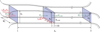
We consider a simple channel of length
 $L_{c}$
with a flat bottom and constant width
 $W_{c}$
, as shown in the schematic in figure 1. Tidal head is the only driving force considered, as in Bryden & Couch (Reference Bryden and Couch2007), and is given as the difference between the water column heights at the channel inlet and outlet (
 $\unicode[STIX]{x0394}h=h_{1}-h_{5}$
). It is assumed that the tidal head is unaffected by the presence of turbines in the channel. The upstream channel flow velocity is assumed to be uniform in the vertical direction, and is given by
 $U_{1}$
when no turbines are present. The Froude number of the flow is defined as
 $Fr=U_{1}/\sqrt{gh_{1}}$
, where
 $g$
is acceleration due to gravity. We only consider the quasi-steady case, i.e. time variation of the tidal head is not modelled. Furthermore, we assume that on both sides of the channel (before the inlet and after the outlet) there are large basins of water.
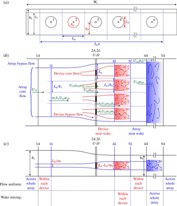
The turbines are modelled as actuator discs, each with diameter
 $L_{d}$
and area
 $A_{d}$
, and are placed with intra-turbine spacing
 $L_{a}$
as shown in figure 2(a). They are tuned by adjusting the local induction factor ‘
 $a$
’ (defined in (2.31)), which is a measure of the flow resistance of each turbine. The fraction of the channel inlet area occupied by the turbines is called the global blockage (
 $B_{g}=nA_{d}/W_{c}h_{1}$
), where
 $n$
is the number of turbines in the array. The fraction of the channel inlet area occupied by the whole array is called the array blockage (
 $B_{a}=nL_{a}L_{d}/W_{c}h_{1}$
). The fraction of each turbine’s local flow passage area that is occupied by the turbine is called the local blockage (
 $B_{l}=A_{d}/L_{a}L_{d}=B_{g}/B_{a}$
).
The power extracted per turbine (
 $P_{D}$
) is non-dimensionalised by the kinetic energy that would pass through the area occupied by each turbine if the turbines were not present (
 $(1/2)\unicode[STIX]{x1D70C}U_{1}^{3}A_{d}$
). The fraction of this available power extracted per turbine is called the global power coefficient and is given as:
 $$\begin{eqnarray}C_{PG}=\frac{P_{D}}{{\textstyle \frac{1}{2}}\unicode[STIX]{x1D70C}U_{1}^{3}A_{d}}=\frac{nP_{D}}{{\textstyle \frac{1}{2}}\unicode[STIX]{x1D70C}U_{1}^{3}nA_{d}}.\end{eqnarray}$$
An analytical model for a tidal array in the channel described above is obtained by conserving mass, momentum and energy in the axial direction at the channel, array and device scales. In order to close the model, additional equations are obtained from empirical correlations. The hydrostatic approximation, i.e. that the pressure at any point can be expressed in terms of the water column height above that point plus the atmospheric pressure (
 $p_{a}$
), is used for obtaining the local pressure at different points in the domain. This approximation is valid as long as there is no significant flow in the vertical direction.
A three-dimensional view of the whole channel showing key parameters. The tidal head (
 $\unicode[STIX]{x0394}h=h_{1}-h_{5}$
) is assumed to be the only driving term in the channel.

The (a) front, (b) top and (c) side views of the tidal array with velocity and length scales shown at key locations. (a) Shows that
 $n$
equi-spaced turbines are arranged in the centre of the channel. (b) Shows the array-scale and device-scale core and bypass flows. (c) Shows the free surface deformation along the channel.

2.1 Channel-scale conservation equations
In the absence of turbines, the axial velocity profile is assumed to be uniform in the vertical and cross-span directions. The mass and momentum conservation equations across the small axial element of length
 $\text{d}x$
shown in figure 1, which must be satisfied under all conditions, are:
 $$\begin{eqnarray}\displaystyle & \displaystyle W_{c}h(x)U(x)=W_{c}h(x+\text{d}x)U(x+\text{d}x)\;\Longrightarrow \;h(x)\frac{\text{d}U}{\text{d}x}=-U(x)\frac{\text{d}h}{\text{d}x}, & \displaystyle\end{eqnarray}$$
 $$\begin{eqnarray}\displaystyle & & \displaystyle W_{c}\int _{0}^{h(x)}[p_{a}+\unicode[STIX]{x1D70C}g(h(x)-y)]\,\text{d}y-W_{c}\int _{0}^{h(x+\text{d}x)}[p_{a}+\unicode[STIX]{x1D70C}g(h(x+\text{d}x)-y)]\,\text{d}y\nonumber\\ \displaystyle & & \displaystyle \qquad -\,W_{c}p_{a}(h(x)-h(x+\text{d}x))-W_{c}E_{\unicode[STIX]{x0394}h}\unicode[STIX]{x1D6FF}_{xe}\,\text{d}x-W_{c}\unicode[STIX]{x1D70F}_{w}\,\text{d}x\nonumber\\ \displaystyle & & \displaystyle \quad =W_{c}\unicode[STIX]{x1D70C}U(x+\text{d}x)^{2}h(x+\text{d}x)-W_{c}\unicode[STIX]{x1D70C}U(x)^{2}h(x).\end{eqnarray}$$
In the momentum equation, the first three terms are the pressure force terms,
 $E_{\unicode[STIX]{x0394}h}\unicode[STIX]{x1D6FF}_{xe}$
is the kinetic energy loss term,
 $\unicode[STIX]{x1D70F}_{w}$
is the seabed friction force per unit area and the two terms on the right-hand side are the inertial terms. The kinetic energy loss term (
 $E_{\unicode[STIX]{x0394}h}\unicode[STIX]{x1D6FF}_{xe}$
) and seabed friction (
 $\unicode[STIX]{x1D70F}_{w}$
) are also included in the models given by Garrett & Cummins (Reference Garrett and Cummins2005) and Bryden & Couch (Reference Bryden and Couch2007) and together they make up the inherent channel drag.
To understand the origin of the kinetic energy loss term, consider the fact that flow enters the channel from a very large basin. It, therefore, has a very small velocity before the inlet. The flow then gains kinetic energy, which is proportional to the square of the channel flow velocity at inlet (
 $U_{1}$
). This gain, which is given as
 $W_{c}\int _{x_{1}}^{x_{5}}E_{\unicode[STIX]{x0394}h}\unicode[STIX]{x1D6FF}_{xe}\,\text{d}x\approx W_{c}(h_{1}/2)\unicode[STIX]{x1D70C}U_{1}^{2}$
, must come at the cost of tidal head. Here, the delta function,
 $\unicode[STIX]{x1D6FF}_{xe}$
, signifies that we account for this term at the channel exit (location 5).
The seabed friction term is commonly taken to be proportional to the square of the flow velocity as
 $\unicode[STIX]{x1D70F}_{w}=\unicode[STIX]{x1D70C}f_{1}U(x)^{2}$
, where
 $f_{1}$
is a non-dimensional friction coefficient which is assumed to be constant throughout the channel. The channel modelled here has a constant width and the tidal head drop (
 $\unicode[STIX]{x0394}h$
) is usually small. Consequently,
 $U(x)$
does not change much throughout the channel (see (2.3)). So we further simplify the seabed friction to
 $\unicode[STIX]{x1D70F}_{w}=\unicode[STIX]{x1D70C}f_{1}U_{1}^{2}$
.
The models for the two terms of the inherent channel drag are inserted into (2.3) along with (2.2). The resulting equation is then integrated to give a relationship between the undisturbed channel flow velocity (
 $U_{1}$
), the tidal head term (
 $\unicode[STIX]{x0394}h$
) and the drag terms (
 $f=f_{1}L_{c}+h_{1}/2$
):
 $$\begin{eqnarray}U_{1}^{2}=\frac{g\unicode[STIX]{x0394}h{\displaystyle \frac{h_{1}+h_{5}}{2}}}{{\displaystyle \frac{h_{1}}{h_{5}}}\unicode[STIX]{x0394}h+f}\;\Longrightarrow \;Fr^{2}=\frac{U_{1}^{2}}{gh_{1}}=\frac{\unicode[STIX]{x0394}H(1+H_{5})}{C_{f}},\end{eqnarray}$$
where
 $C_{f}=2[\unicode[STIX]{x0394}h/h_{5}+f/h_{1}]$
is the inherent channel drag coefficient and
 $\unicode[STIX]{x0394}H=\unicode[STIX]{x0394}h/h_{1}$
and
 $H_{5}=h_{5}/h_{1}$
are the non-dimensional tidal head drop and channel outlet water column height, respectively.
In the presence of a turbine array at one location (say
 $x_{T}$
) in the channel, the momentum equation (2.3) is modified such that the thrust imparted by turbines (
 $T_{A}$
) is added to the equation as shown by the bold term below:
 $$\begin{eqnarray}\displaystyle & & \displaystyle W_{c}\int _{0}^{h(x)}[p_{a}+\unicode[STIX]{x1D70C}g(h(x)-y)]\,\text{d}y-W_{c}\int _{0}^{h(x+\text{d}x)}[p_{a}+\unicode[STIX]{x1D70C}g(h(x+\text{d}x)-y)]\,\text{d}y\nonumber\\ \displaystyle & & \displaystyle \qquad -\,W_{c}p_{a}(h(x)-h(x+\text{d}x))-W_{c}E_{\unicode[STIX]{x0394}h}\unicode[STIX]{x1D6FF}_{xe}\,\text{d}x-W_{c}\unicode[STIX]{x1D70F}_{w}\,\text{d}x-\boldsymbol{T}_{\boldsymbol{A}}\unicode[STIX]{x1D6FF}(\boldsymbol{x}-\boldsymbol{x}_{\boldsymbol{T}})\,\mathbf{d}\boldsymbol{x}\nonumber\\ \displaystyle & & \displaystyle \quad =W_{c}\unicode[STIX]{x1D70C}U(x+\text{d}x)^{2}h(x+\text{d}x)-W_{c}\unicode[STIX]{x1D70C}U(x)^{2}h(x).\end{eqnarray}$$
The cross-stream variation in the axial flow velocity caused by the array will affect the friction term in the channel
 $W_{c}\unicode[STIX]{x1D70F}_{w}\,\text{d}x$
. This effect is ignored here for now, but it will be considered in § 2.3, after the array-scale dynamics is introduced. Integrating this modified momentum equation along the length of the channel gives:
 $$\begin{eqnarray}U_{1nd}^{2}=\frac{U_{1d}^{2}}{U_{1}^{2}}=1-\frac{T_{A}}{{\textstyle \frac{1}{2}}\unicode[STIX]{x1D70C}U_{1}^{2}nA_{d}}\frac{nA_{d}}{W_{c}h_{1}}\frac{1}{C_{f}},\end{eqnarray}$$
where
 $U_{1d}$
is the reduced upstream channel flow velocity and
 $U_{1nd}$
is its non-dimensional form. The term
 $T_{A}/((\unicode[STIX]{x1D70C}U_{1}^{2}nA_{d})/2)$
is a non-dimensional form of the thrust imparted by the turbines and will be referred to as the global thrust coefficient (
 $C_{TG}$
). Equation (2.6) can then be rewritten as:
 $$\begin{eqnarray}U_{1nd}^{2}=1-C_{TG}B_{g}/C_{f}.\end{eqnarray}$$
This equation shows that the channel flow velocity at the inlet reduces as the thrust imparted by the turbines,
 $C_{TG}$
, increases. The channel-scale conservation equation (2.7) is our first model equation and contains two unknown variables:
 $U_{1nd}$
and
 $C_{TG}$
.
2.1.1 Estimation of
 $C_{f}$

The inherent channel drag coefficient (
 $C_{f}$
) is a channel parameter which governs the effect of added drag from the turbines. In our model, we vary
 $C_{f}$
continuously, but here we give a brief discussion of its physical meaning and of its magnitude in typical marine flows. By assuming that the non-dimensional tidal head drop is small (
 $\unicode[STIX]{x0394}H\ll 1$
– this will be true even in shallow channels), the inherent channel drag coefficient is approximated as:
 $$\begin{eqnarray}C_{f}=2\frac{\unicode[STIX]{x0394}H}{H_{5}}+2\frac{f_{1}L_{c}+h_{1}/2}{h_{1}}\approx 1+2\,\frac{f_{1}L_{c}}{h_{1}},\end{eqnarray}$$
where
 $f_{1}$
depends up on the roughness of the seabed. This estimation of
 $C_{f}$
is similar to that of Bryden & Couch (Reference Bryden and Couch2007), who use a different friction model. They give the coefficient as
 $C_{f}=1+2gn_{m}^{2}L_{c}/R_{d}^{(4/3)}$
, where
 $R_{d}$
is the hydraulic radius of the channel and
 $n_{m}$
is the Manning seabed friction coefficient. For the channel considered in Bryden & Couch (Reference Bryden and Couch2007) (where
 $L_{c}=4000~\text{m}$
,
 $W_{c}=500~\text{m}$
,
 $h_{1}=40~\text{m}$
and
 $n_{m}=0.025~\text{sm}^{-1/3}$
), the value of
 $C_{f}$
is approximately 1.44 (or
 $1/C_{f}\approx 0.70$
).
Equation (2.7) shows that small values of
 $C_{f}$
are desirable, because smaller
 $C_{f}$
means larger
 $U_{1}$
for a given
 $\unicode[STIX]{x0394}H$
and therefore greater available kinetic energy for a given tidal head. For channels with small
 $C_{f}$
, the drag added by the turbines is comparable to the inherent channel drag. This implies that the added drag reduces the channel flow velocity at inlet, i.e.
 $U_{1nd}<1$
. For those channels with large
 $C_{f}$
, the drag added by the turbines is negligible compared to the inherent channel drag. This implies that the added drag has no effect on the upstream channel flow velocity, i.e.
 $U_{1nd}\approx 1$
.
2.2 Array-scale conservation equations
Figure 2 shows the (a) front, (b) top and (c) side views of the turbine array. The front view shows that
 $n$
turbines are arranged symmetrically in the centre of the channel. They are regularly spaced with distance
 $L_{a}$
between each other, and each turbine is represented as an actuator disc of diameter
 $L_{d}$
(area
 $A_{d}=\unicode[STIX]{x03C0}L_{d}^{2}/4$
). The height of the centre of turbines from the bottom of the channel is
 $h_{T}$
, but this term will not appear in the final equations because the upstream velocity profile is assumed to be uniform in the vertical direction. The array inlet and outlet are marked as
 $1A$
and
 $5A$
, respectively. We assume that the tidal array is close to the channel inlet such that axial locations 1 in figure 1 and
 $1A$
in figure 2 coincide. We also assume that the channel is long enough that location
 $5A$
is upstream of location 5, which means that all the wake mixing behind the array is completed before the channel outlet.
The flow that passes through each turbine is called the device-scale core flow and the flow that passes between the turbines is called the device-scale bypass flow. Similarly, the flow that passes through the array is called the array-scale core flow (this flow includes the device-scale core and bypass flows) and the flow that passes between the array and the channel boundaries is called the array-scale bypass flow. The wake mixing regions between
 $4L$
and
 $5L$
(device-scale far-wake mixing) and between
 $4A$
and
 $5A$
(array-scale far-wake mixing) are shaded in the figure. It is assumed in the model that wake mixing is limited to the shaded regions and that the device-scale and array-scale wake mixing processes happen in separate regions. In reality, however, much of the array-scale wake mixing in the vertical direction is likely to happen between
 $4L$
and
 $5L$
(array-scale near-wake region) as opposed to between
 $4A$
and
 $5A$
. These assumptions, of separate regions of wake mixing for the device and array scales and of the absence of wake mixing in the near-wake region, are limitations of the present model and their implications are discussed in § 4.
At
 $1A$
, both the velocity (
 $U_{1nd}$
) and channel height (
 $h_{1}$
) are uniform across the whole channel width. The locations immediately upstream and downstream of the turbines are marked as
 $U$
and
 $D$
, respectively. Neither the velocity nor the channel height are uniform at these locations. The average values of the array-scale dynamical variables between
 $U$
and
 $D$
are denoted by the subscript
 $2A$
. The location downstream of turbines where the channel height (
 $h_{4}$
) is uniform across the channel width but the flow velocity is still varying is marked as
 $4A$
. The location far downstream where the channel height (
 $h_{5}$
) and flow velocity are both uniform is marked as
 $5A$
.
At first, we neglect seabed friction at the array scale and derive the conservation equations. Mass conservation between
 $1A$
and
 $4A$
gives:
 $$\begin{eqnarray}\displaystyle U_{1d}h_{1}W_{c} & = & \displaystyle U_{1d}\unicode[STIX]{x1D6FD}_{4A}(h_{4}W_{c}-A_{4Ac})+U_{1d}\unicode[STIX]{x1D6FC}_{4A}A_{4Ac}\nonumber\\ \displaystyle & & \displaystyle \;\Longrightarrow \;1=H_{4}\unicode[STIX]{x1D6FD}_{4A}+\unicode[STIX]{x1D6FC}_{2A}B_{a}\left(1-\frac{\unicode[STIX]{x1D6FD}_{4A}}{\unicode[STIX]{x1D6FC}_{4A}}\right),\end{eqnarray}$$
where
 $\unicode[STIX]{x1D6FC}_{2A}$
is the ratio of the core flow velocity at
 $2A$
to the upstream flow velocity at
 $1A$
,
 $\unicode[STIX]{x1D6FC}_{4A}$
and
 $\unicode[STIX]{x1D6FD}_{4A}$
are the ratios of the core and bypass flow velocities, respectively, at
 $4A$
to the upstream flow velocity at
 $1A$
. Finally,
 $A_{4Ac}=nL_{a}L_{d}(\unicode[STIX]{x1D6FC}_{2A}/\unicode[STIX]{x1D6FC}_{4A})$
is the array core flow area at
 $4A$
, and
 $H_{4}=h_{4}/h_{1}$
.
Considering energy conservation in the array core flow region between
 $1A$
and
 $4A$
gives:
 $$\begin{eqnarray}\displaystyle & & \displaystyle \frac{1}{2}\unicode[STIX]{x1D70C}U_{1d}^{3}\unicode[STIX]{x1D6FC}_{4A}^{3}A_{4Ac}+U_{1d}\unicode[STIX]{x1D6FC}_{4A}\frac{A_{4Ac}}{L_{d4}}\int _{h_{T}-L_{d4}/2}^{h_{T}+L_{d4}/2}[p_{a}+\unicode[STIX]{x1D70C}g(h_{4}-y)]\,\text{d}y+P_{A}\nonumber\\ \displaystyle & & \displaystyle \quad =\frac{1}{2}\unicode[STIX]{x1D70C}U_{1d}^{3}A_{1Ac}+U_{1d}\frac{A_{1Ac}}{L_{d1}}\int _{h_{T}-L_{d1}/2}^{h_{T}+L_{d1}/2}[p_{a}+\unicode[STIX]{x1D70C}g(h_{1}-y)]\,\text{d}y\nonumber\\ \displaystyle & & \displaystyle \qquad \;\Longrightarrow \;U_{1nd}^{2}(1-\unicode[STIX]{x1D6FC}_{4A}^{2})+\frac{2}{Fr^{2}}(1-H_{4})=B_{l}C_{TG},\end{eqnarray}$$
where
 $A_{1Ac}=nL_{a}L_{d}\unicode[STIX]{x1D6FC}_{2A}$
is the array core flow area at
 $1A$
,
 $L_{d1}$
and
 $L_{d4}$
are the vertical extents of the array core flow regions at
 $1A$
and
 $4A$
, respectively, and
 $P_{A}$
is the power extracted from the flow by the array of turbines (given by
 $T_{A}U_{1d}\unicode[STIX]{x1D6FC}_{2A}$
). Note that
 $P_{A}$
is the sum of the useful power extracted by the turbines (
 $nP_{D}=T_{A}U_{1d}\unicode[STIX]{x1D6FC}_{2A}\unicode[STIX]{x1D6FC}_{2L}$
, see § 2.4) and the power dissipated in all the wake mixing regions between
 $4L$
and
 $5L$
.
Energy conservation for the bypass flow can be satisfied by using Bernoulli’s equation, which gives:
 $$\begin{eqnarray}1-H_{4}=\frac{Fr^{2}}{2}U_{1nd}^{2}(\unicode[STIX]{x1D6FD}_{4A}^{2}-1).\end{eqnarray}$$
The momentum conservation equation for the array-scale flow between
 $1A$
and
 $4A$
is given by the relation:
 $$\begin{eqnarray}\displaystyle & & \displaystyle \unicode[STIX]{x1D70C}U_{1d}^{2}h_{1}W_{c}-\unicode[STIX]{x1D70C}U_{1d}^{2}\unicode[STIX]{x1D6FD}_{4A}^{2}(h_{4}W_{c}-A_{4Ac})-\unicode[STIX]{x1D70C}U_{1d}^{2}\unicode[STIX]{x1D6FC}_{4A}^{2}A_{4Ac}=p_{a}(h_{1}-h_{4})W_{c}\nonumber\\ \displaystyle & & \displaystyle \quad +\,T_{A}+W_{c}\int _{0}^{h_{4}}[p_{a}+\unicode[STIX]{x1D70C}gy]\,\text{d}y-W_{c}\int _{0}^{h_{1}}[p_{a}+\unicode[STIX]{x1D70C}gy]\,\text{d}y\nonumber\\ \displaystyle & & \displaystyle \quad \;\Longrightarrow \;2U_{1nd}^{2}[1-\unicode[STIX]{x1D6FD}_{4A}+\unicode[STIX]{x1D6FC}_{2A}B_{a}(\unicode[STIX]{x1D6FD}_{4A}-\unicode[STIX]{x1D6FC}_{4A})]=C_{TG}B_{g}-\frac{1}{Fr^{2}}(1-H_{4}^{2}).\end{eqnarray}$$
The array-scale conservation equations, therefore, give us four additional equations, ((2.9)–(2.12)), and four additional unknown variables, which are
 $H_{4}$
,
 $\unicode[STIX]{x1D6FC}_{2A}$
,
 $\unicode[STIX]{x1D6FC}_{4A}$
and
 $\unicode[STIX]{x1D6FD}_{4A}$
. Together with the equation from the channel scale (2.7), there are now five equations and six unknown variables.
2.3 Channel and array-scale friction terms
The installation of a tidal array in a channel causes an increase in the total channel drag, which is referred to as added drag in this paper. This added drag comes from two sources. The first is directly, from the drag imparted by the turbines on the flow, its effect appears as
 $C_{TG}$
in (2.7). The second is indirectly, from the cross-stream axial flow variations caused by the tidal array. The friction force in a channel depends on the flow velocity and here it is modelled to be proportional to the square of the velocity as explained in § 2.1. Consequently, the cross-stream axial flow variations, if significant, cause an increase in the friction force in the channel. This second source of added drag is non-negligible only when the array length is comparable to the channel length because only then the cross-stream axial flow variations persist for a significant proportion of the channel length to affect the total friction force. When the array length is long, such that it is comparable to the channel length, then another effect that can come into play is the friction at the array scale. In this subsection, we will include the effects of (i) the tidal array-induced axial flow variations on the friction force in the channel and (ii) the friction force on the array-scale dynamics.
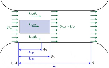
Figure 3 shows a top view schematic of the channel-scale flow with the tidal array represented as a box with blockage area ratio
 $B_{a}$
and length
 $L_{15A}$
. As mentioned before, the change in the water column height along the axial direction is usually small, so we assume that the average velocity remains constant at every axial location and take it to be
 $U_{1d}$
everywhere for the purpose of estimating the friction force. We make a further approximation by using average array bypass and core flow velocities throughout the array length (
 $L_{15A}$
). The maximum array bypass flow velocity factor is
 $\unicode[STIX]{x1D6FD}_{4A}$
, which is achieved at location
 $4A$
, and the minimum is 1, which is achieved at locations
 $1A$
and
 $5A$
. The average array bypass flow from
 $1A$
to
 $5A$
(
 $\unicode[STIX]{x1D6FD}_{b}$
), therefore, is modelled approximately as:
 $\unicode[STIX]{x1D6FD}_{b}=0.5(1+\unicode[STIX]{x1D6FD}_{4A})$
. In order to satisfy the conservation of mass, the average core flow from
 $1A$
to
 $5A$
(
 $\unicode[STIX]{x1D6FC}_{c}$
) is given by the relation below.
 $$\begin{eqnarray}\unicode[STIX]{x1D6FC}_{c}B_{a}+0.5(\unicode[STIX]{x1D6FD}_{4A}+1)(1-B_{a})=1.\end{eqnarray}$$
Top view schematic of the channel-scale flow with the tidal array represented as a box with blockage area ratio
 $B_{a}$
.

The array length (
 $L_{15A}$
) varies with the local turbine arrangement (
 $B_{l}$
). On the one hand, for
 $B_{l}\approx 0$
, i.e. when devices are very far apart from each other, there is very little interaction between the devices and the array-scale wake length will be close to the wake length for a single device. On the other hand, for
 $B_{l}\approx 1$
, i.e. when devices are almost touching, the flow will see the devices as one large device and the array-scale wake length will be scaled accordingly. We assume a simple linear relation for
 $L_{15A}$
at intermediate values of
 $B_{l}$
as:
 $$\begin{eqnarray}L_{15A}=L_{Array}\left(\frac{(n-1)B_{l}+1}{n}\right),\end{eqnarray}$$
where
 $L_{Array}$
is the maximum length of the array that is achieved when
 $B_{l}=1$
and
 $L_{Array}$
itself depends on the global blockage. It will increase monotonically with
 $B_{g}$
for a given channel, and we assume this increase will also be linear. In this paper, the channel length is always given in terms of the ratio
 $L_{A/C}=L_{Array}/L_{c}$
at a given
 $B_{g}$
, and this ratio (
 $L_{A/C}$
) changes linearly with
 $B_{g}$
. For example, if the channel length is given as
 $L_{A/C}=0.5$
at
 $B_{g}=0.2$
, then for this channel
 $L_{A/C}=0.25$
at
 $B_{g}=0.1$
.
Based on the above assumptions, the friction force across the channel is given as:
 $$\begin{eqnarray}\displaystyle W_{c}\int _{0}^{L_{c}}\unicode[STIX]{x1D70F}_{w}\,\text{d}x & = & \displaystyle W_{c}\unicode[STIX]{x1D70C}f_{1}U_{1d}^{2}(L_{c}-L_{15A})+W_{c}B_{a}\unicode[STIX]{x1D70C}f_{1}U_{1d}^{2}\unicode[STIX]{x1D6FC}_{c}^{2}L_{15A}\nonumber\\ \displaystyle & & \displaystyle +\,W_{c}(1-B_{a})\unicode[STIX]{x1D70C}f_{1}U_{1d}^{2}\left(\frac{1+\unicode[STIX]{x1D6FD}_{4A}}{2}\right)^{2}L_{15A}\nonumber\\ \displaystyle & = & \displaystyle W_{c}\unicode[STIX]{x1D70C}f_{1}U_{1d}^{2}\left[L_{c}+L_{15A}\left(B_{a}\unicode[STIX]{x1D6FC}_{c}^{2}+(1-B_{a})\left(\frac{1+\unicode[STIX]{x1D6FD}_{4A}}{2}\right)^{2}-1\right)\right].\qquad\end{eqnarray}$$
This friction term is then inserted in (2.5), and the resulting equation after integration and non-dimensionalisation is given as:
 $$\begin{eqnarray}U_{1nd}^{2}=\frac{C_{f}}{C_{f}+C_{fm}}-\frac{C_{TG}B_{g}}{C_{f}+C_{fm}},\end{eqnarray}$$
where
 $C_{fm}=(2f_{1}L_{15A}/h_{1})(B_{a}\unicode[STIX]{x1D6FC}_{c}^{2}+(1-B_{a})((1+\unicode[STIX]{x1D6FD}_{4A})/2)^{2}-1)$
is the non-dimensional tidal array-induced increase in the channel friction force. A higher value of
 $C_{fm}$
means a higher reduction in the incoming flow velocity
 $U_{1nd}$
. It can be seen that
 $C_{fm}$
is higher when the bypass flow coefficient
 $\unicode[STIX]{x1D6FD}_{4A}$
and the array length
 $L_{15A}$
are higher; both of these terms increase with
 $B_{l}$
and
 $B_{g}$
.
In order to include the friction terms in the array-scale conservation equations, we also need an estimation of the length from
 $1A$
to
 $4A$
(
 $L_{14A}$
) as a fraction of
 $L_{15A}$
. The length from
 $2A$
to
 $4A$
, which is the near-wake length, is known to be 2–4 times the turbine diameter (Mehta et al.
Reference Mehta, van Zuijlen, Koren, Holierhoek and Bijl2014), and the length from
 $2A$
to
 $5A$
, which includes the near as well as the far-wake lengths, is known to be 6–10 times the turbine diameter (Mehta et al.
Reference Mehta, van Zuijlen, Koren, Holierhoek and Bijl2014). The length from
 $1A$
to
 $2A$
is usually taken to be twice the turbine diameter (Porté-Agel et al.
Reference Porté-Agel, Wu, Lu and Conzemius2011). Based on these numbers,
 $L_{14A}$
is 0.5–0.75 times
 $L_{15A}$
. In this paper, we assume
 $L_{14A}=0.7L_{15A}$
. The friction force from
 $1A$
to
 $4A$
is then given as:
 $$\begin{eqnarray}W_{c}\int _{0}^{L_{14A}}\unicode[STIX]{x1D70F}_{w}\,\text{d}x=W_{c}\unicode[STIX]{x1D70C}f_{1}U_{1d}^{2}L_{14A}\left(B_{a}\unicode[STIX]{x1D6FC}_{c}^{2}+(1-B_{a})\left(\frac{1+\unicode[STIX]{x1D6FD}_{4A}}{2}\right)^{2}\right).\end{eqnarray}$$
This term is substituted into (2.12) (momentum conservation between
 $1A$
and
 $4A$
), which becomes:
 $$\begin{eqnarray}2U_{1nd}^{2}[1-\unicode[STIX]{x1D6FD}_{4A}+\unicode[STIX]{x1D6FC}_{2A}B_{a}(\unicode[STIX]{x1D6FD}_{4A}-\unicode[STIX]{x1D6FC}_{4A})]=U_{1nd}^{2}C_{fm2}+C_{TG}B_{g}-\frac{1}{Fr^{2}}(1-H_{4}^{2}),\end{eqnarray}$$
where
 $C_{fm2}=(2f_{1}L_{14A}/h_{1})(B_{a}\unicode[STIX]{x1D6FC}_{c}^{2}+(1-B_{a})((1+\unicode[STIX]{x1D6FD}_{4A})/2)^{2})$
is the non-dimensional friction force at the array scale. This term increases with
 $\unicode[STIX]{x1D6FD}_{4A}$
,
 $L_{14A}$
and
 $f_{1}$
.
This second additional friction term (
 $C_{fm2}$
) also affects the array-scale core and bypass flow energy equations. The effect of friction is to create shear in the entire flow such that energy gets dissipated everywhere. This dissipation is given as the friction force multiplied by the velocity flux. This means that the dissipation in the array-scale core and bypass flow will be given by multiplying the friction force,
 $C_{fm2}$
, by
 $U_{1d}\unicode[STIX]{x1D6FC}_{2A}B_{a}W_{c}h_{1}$
and
 $U_{1d}W_{c}h_{1}(1-\unicode[STIX]{x1D6FC}_{2A}B_{a})$
, respectively. The energy equations in the array-scale core and bypass flows between
 $1A$
and
 $4A$
, which were given by (2.10) and (2.11), respectively, are now given as:
 $$\begin{eqnarray}\displaystyle & \displaystyle U_{1nd}^{2}(1-\unicode[STIX]{x1D6FC}_{4A}^{2})+\frac{2}{Fr^{2}}(1-H_{4})=B_{l}C_{TG}+U_{1nd}^{2}C_{fm2}, & \displaystyle\end{eqnarray}$$
 $$\begin{eqnarray}\displaystyle & \displaystyle 1-H_{4}=\frac{Fr^{2}}{2}U_{1nd}^{2}[(\unicode[STIX]{x1D6FD}_{4A}^{2}-1)+C_{fm2}], & \displaystyle\end{eqnarray}$$
where (2.20) is equivalent to the Darcy–Weisbach equation, which is a phenomenological equation used for estimating head loss in a pipe or a channel with wall friction. This equation also shows that
 $C_{fm2}$
causes a reduction in
 $H_{4}$
, and therefore makes the flow through the turbines faster and thus increases the power generation. It seems counter-intuitive that friction is causing an increase in power generation. However, it must be noted that for a given tidal head, the increase in channel friction will also cause a reduction in the incoming flow velocity (2.16) and so the overall effect will be a reduction in power generation.
Lastly, we modify the definition of the global power coefficient (
 $C_{PG}$
), given in (2.1), to:
 $$\begin{eqnarray}C_{PG}=\frac{P_{D}}{{\textstyle \frac{1}{2}}\unicode[STIX]{x1D70C}U_{5A}^{3}A_{d}}=\frac{nP_{D}}{{\textstyle \frac{1}{2}}\unicode[STIX]{x1D70C}U_{5A}^{3}nA_{d}},\end{eqnarray}$$
where
 $U_{5A}$
is the flow velocity through location
 $5A$
when turbines are not present in the channel. This change is to account for the increase in the flow through the turbines because of their placement in the channel.
The introduction of these two effects – the tidal array-induced increase in the channel friction and the friction at the array scale – therefore gives us an additional variable
 $\unicode[STIX]{x1D6FC}_{c}$
and an additional equation (2.13). Further to this, the channel and array-scale momentum equations, and the array-scale core and bypass flow energy equations are replaced by (2.16), (2.18), (2.19) and (2.20), respectively.
2.4 Device-scale conservation equations
The device scale is between locations
 $1L$
and
 $5L$
as marked in figure 2. We assume that the length of the device-scale region is small enough for the effects of friction to be ignored. The flow through the individual devices is separated by the dashed lines and comprises of the device-scale core and bypass flows (shown in figure 2
b). The dimensions of the device-scale flow width and vertical height at locations
 $1L$
and
 $4L$
are given in terms of the array-scale area factors (
 $m_{1},k_{1},m_{4}$
and
 $k_{4}$
) (shown in figure 2
b,c). These factors are modelled empirically in § 2.5. At the upstream location,
 $1L$
, the velocity (
 $U_{1L}=m_{1}k_{1}U_{1d}\unicode[STIX]{x1D6FC}_{2A}$
) and channel height (
 $h_{1L}$
) are both uniform across the local passage. Locations
 $U$
and
 $D$
are the positions immediately upstream and downstream of the turbines, respectively. The average values of the device-scale variables at the turbine location have subscript
 $2L$
. The location downstream of the turbines where the channel height (
 $h_{4L}$
) is uniform across the local passage width (
 $L_{d}/k_{4}$
) but the flow velocity is still varying is marked
 $4L$
. Location
 $5L$
is further downstream in the channel after the device-scale wake mixing is completed. The channel height and flow velocity are both uniform across the local passage width at this location.
Mass conservation between
 $1L$
and
 $4L$
gives:
 $$\begin{eqnarray}\unicode[STIX]{x1D6FD}_{4L}=\frac{1-\unicode[STIX]{x1D6FC}_{2L}B_{l}}{1-{\displaystyle \frac{\unicode[STIX]{x1D6FC}_{2L}}{\unicode[STIX]{x1D6FC}_{4L}}}B_{l}},\end{eqnarray}$$
where
 $\unicode[STIX]{x1D6FC}_{2L}$
is the local core flow velocity coefficient at the array location and
 $\unicode[STIX]{x1D6FC}_{4L}$
and
 $\unicode[STIX]{x1D6FD}_{4L}$
are the local core and bypass flow velocity coefficients at
 $4L$
, respectively.
Energy conservation in the local core flow between
 $1L$
and
 $4L$
gives:
 $$\begin{eqnarray}\displaystyle & & \displaystyle \frac{1}{2}\unicode[STIX]{x1D70C}(m_{4}k_{4}U_{1d}\unicode[STIX]{x1D6FC}_{2A}\unicode[STIX]{x1D6FC}_{4L})^{3}A_{4Lc}-\frac{1}{2}\unicode[STIX]{x1D70C}(m_{1}k_{1}U_{1d}\unicode[STIX]{x1D6FC}_{2A})^{3}A_{1Lc}+P_{D}\nonumber\\ \displaystyle & & \displaystyle \quad =m_{1}k_{1}U_{1d}\unicode[STIX]{x1D6FC}_{2A}A_{1Lc}p_{avg1L}-m_{4}k_{4}U_{1d}\unicode[STIX]{x1D6FC}_{2A}\unicode[STIX]{x1D6FC}_{4L}A_{4Lc}p_{avg4L}\nonumber\\ \displaystyle & & \displaystyle \qquad \;\Longrightarrow \;U_{1nd}^{2}\unicode[STIX]{x1D6FC}_{2A}^{2}[(m_{1}k_{1})^{2}-(m_{4}k_{4})^{2}\unicode[STIX]{x1D6FC}_{4L}^{2}]+\frac{2}{Fr^{2}}(H_{1L}-H_{4L})=C_{TG},\end{eqnarray}$$
where
 $P_{D}$
is the useful power extracted from the flow by a single turbine and
 $H_{1L}=h_{1L}/h_{1}$
and
 $H_{4L}=h_{4L}/h_{1}$
are the non-dimensional heights across the device scale at
 $1L$
and
 $4L$
, respectively.
 $A_{1Lc}$
and
 $A_{4Lc}$
are local core flow areas at
 $1L$
and
 $4L$
, respectively, and are given as:
 $$\begin{eqnarray}A_{1Lc}=\frac{A_{d}}{m_{1}k_{1}}\unicode[STIX]{x1D6FC}_{2L},\quad A_{4Lc}=\frac{A_{d}}{m_{4}k_{4}}\frac{\unicode[STIX]{x1D6FC}_{2L}}{\unicode[STIX]{x1D6FC}_{4L}}.\end{eqnarray}$$
The terms
 $p_{avg1L}$
and
 $p_{avg4L}$
are the average pressures in the local flow passage at
 $1L$
and
 $4L$
, respectively, and are approximated by the hydrostatic pressure at the midpoint of the core flow at
 $1L$
and
 $4L$
as:
 $$\begin{eqnarray}p_{avg1L}=[p_{a}+\unicode[STIX]{x1D70C}g(h_{1L}-h_{T})],\quad p_{avg4L}=[p_{a}+\unicode[STIX]{x1D70C}g(h_{4L}-h_{T})].\end{eqnarray}$$
Energy conservation in the local bypass flow between
 $1L$
and
 $4L$
gives:
 $$\begin{eqnarray}\displaystyle & & \displaystyle \frac{1}{2}\unicode[STIX]{x1D70C}(m_{4}k_{4}U_{1d}\unicode[STIX]{x1D6FC}_{2A}\unicode[STIX]{x1D6FD}_{4L})^{3}\left(\frac{A_{l}}{m_{4}k_{4}}-A_{4Lc}\right)-\frac{1}{2}\unicode[STIX]{x1D70C}(m_{1}k_{1}U_{1d}\unicode[STIX]{x1D6FC}_{2A})^{3}\left(\frac{A_{l}}{m_{1}k_{1}}-A_{1Lc}\right)\nonumber\\ \displaystyle & & \displaystyle \quad =U_{1d}\unicode[STIX]{x1D6FC}_{2A}\left[m_{1}k_{1}\left(\frac{A_{l}}{m_{1}k_{1}}-A_{1Lc}\right)p_{avg1L}-m_{4}k_{4}\unicode[STIX]{x1D6FC}_{4L}\left(\frac{A_{l}}{m_{4}k_{4}}-A_{4Lc}\right)p_{avg4L}\right]\nonumber\\ \displaystyle & & \displaystyle \qquad \;\Longrightarrow \;\frac{2}{Fr^{2}}(H_{1L}-H_{4L})=U_{1nd}^{2}\unicode[STIX]{x1D6FC}_{2A}^{2}[(m_{4}k_{4}\unicode[STIX]{x1D6FD}_{4L})^{2}-(m_{1}k_{1})^{2}].\end{eqnarray}$$
The term
 $H_{1L}-H_{4L}$
is eliminated by combining the device-scale core flow and bypass flow energy equations ((2.23) and (2.26)). The resulting equation is:
 $$\begin{eqnarray}U_{1nd}^{2}\unicode[STIX]{x1D6FC}_{2A}^{2}(m_{4}k_{4})^{2}[\unicode[STIX]{x1D6FD}_{4L}^{2}-\unicode[STIX]{x1D6FC}_{4L}^{2}]=C_{TG}.\end{eqnarray}$$
Momentum conservation for the local passage between
 $1L$
and
 $4L$
gives:
 $$\begin{eqnarray}\displaystyle T_{D} & = & \displaystyle p_{avg1L}\frac{A_{l}}{m_{1}k_{1}}-p_{avg4L}\frac{A_{l}}{m_{4}k_{4}}+p^{\ast }A_{14L}^{\ast }+\unicode[STIX]{x1D70C}(m_{1}k_{1}U_{1d}\unicode[STIX]{x1D6FC}_{2A})^{2}\frac{A_{l}}{m_{1}k_{1}}\nonumber\\ \displaystyle & & \displaystyle -\,\unicode[STIX]{x1D70C}(m_{4}k_{4}U_{1d}\unicode[STIX]{x1D6FC}_{2A}\unicode[STIX]{x1D6FC}_{4L})^{2}A_{4Lc}-\unicode[STIX]{x1D70C}(m_{4}k_{4}U_{1d}\unicode[STIX]{x1D6FC}_{2A}\unicode[STIX]{x1D6FD}_{4L})^{2}\left(\frac{A_{l}}{m_{4}k_{4}}-A_{4Lc}\right)\nonumber\\ \displaystyle & & \displaystyle \;\Longrightarrow \;\frac{(m_{4}k_{4})^{2}}{2}(\unicode[STIX]{x1D6FD}_{4L}^{2}-\unicode[STIX]{x1D6FC}_{4L}^{2})=\frac{m_{1}k_{1}}{Bl}-m_{4}k_{4}\unicode[STIX]{x1D6FC}_{4L}\unicode[STIX]{x1D6FC}_{2L}-\frac{m_{4}k_{4}\unicode[STIX]{x1D6FD}_{4L}^{2}}{Bl}\nonumber\\ \displaystyle & & \displaystyle +\,m_{4}k_{4}\unicode[STIX]{x1D6FD}_{4L}^{2}\frac{\unicode[STIX]{x1D6FC}_{2L}}{\unicode[STIX]{x1D6FC}_{4L}}+\frac{1}{2Blm_{4}k_{4}}[(m_{4}k_{4}\unicode[STIX]{x1D6FD}_{4L})^{2}-(m_{1}k_{1})^{2}].\end{eqnarray}$$
The term
 $p^{\ast }A_{14L}^{\ast }$
is the pressure force term arising from the non-zero axial projection of the lateral surface area between
 $1L$
and
 $4L$
. This term is modelled in the same way as in Nishino & Willden (Reference Nishino and Willden2013):
 $$\begin{eqnarray}p_{avg1L}\frac{A_{l}}{m_{1}k_{1}}+p^{\ast }A_{14L}^{\ast }=p_{avg1L}\frac{A_{l}}{m_{4}k_{4}}.\end{eqnarray}$$
The resulting equation then is written as:
 $$\begin{eqnarray}\displaystyle \frac{(m_{4}k_{4})^{2}}{2}(\unicode[STIX]{x1D6FD}_{4L}^{2}-\unicode[STIX]{x1D6FC}_{4L}^{2}) & = & \displaystyle \frac{m_{1}k_{1}}{B_{l}}-m_{4}k_{4}\unicode[STIX]{x1D6FC}_{4L}\unicode[STIX]{x1D6FC}_{2L}-\frac{m_{4}k_{4}\unicode[STIX]{x1D6FD}_{4L}^{2}}{B_{l}}+m_{4}k_{4}\unicode[STIX]{x1D6FD}_{4L}^{2}\frac{\unicode[STIX]{x1D6FC}_{2L}}{\unicode[STIX]{x1D6FC}_{4L}}\nonumber\\ \displaystyle & & \displaystyle +\,\frac{1}{2B_{l}m_{4}k_{4}}[(m_{4}k_{4}\unicode[STIX]{x1D6FD}_{4L})^{2}-(m_{1}k_{1})^{2}].\end{eqnarray}$$
The device-scale conservation equations therefore give us 3 additional model equations, these are (2.22), (2.27) and (2.30). The new variables introduced are
 $\unicode[STIX]{x1D6FC}_{2L}$
,
 $\unicode[STIX]{x1D6FC}_{4L}$
and
 $\unicode[STIX]{x1D6FD}_{4L}$
, as well as the products
 $m_{1}k_{1}$
and
 $m_{4}k_{4}$
which are the array-scale area factors.
Having considered the conservation equations over the channel, array and device scales, we have nine equations and twelve unknown variables. In order to close the equations, we now derive three additional equations based on empirical models. These equations govern the drag of the turbines and the array-scale area factors.
2.5 Empirically modelled equations necessary for closure
The turbines are modelled empirically in terms of a local induction factor (
 $a$
), which is defined as the ratio of the deceleration in the local core flow velocity between
 $1L$
and
 $2L$
to the local core flow velocity at
 $1L$
:
 $$\begin{eqnarray}a=\frac{m_{1}k_{1}\unicode[STIX]{x1D6FC}_{2A}U_{1d}-\unicode[STIX]{x1D6FC}_{2A}\unicode[STIX]{x1D6FC}_{2L}U_{1d}}{m_{1}k_{1}\unicode[STIX]{x1D6FC}_{2A}U_{1d}}=1-\frac{\unicode[STIX]{x1D6FC}_{2L}}{m_{1}k_{1}}.\end{eqnarray}$$
A higher value of induction factor implies that more drag is imparted on the flow by the turbines. This parameter will be used as the turbine tuning parameter in this paper.
The other empirically modelled quantities are the array-scale area factors
 $m_{1}$
,
 $k_{1}$
,
 $m_{4}$
and
 $k_{4}$
. These factors quantify the expansion in the array core flow between
 $1L$
and
 $4L$
. Because these factors only appear as products,
 $m_{1}k_{1}$
and
 $m_{4}k_{4}$
, in the equations, they are modelled together as:
 $$\begin{eqnarray}\left.\begin{array}{@{}c@{}}\displaystyle m_{1}k_{1}=\left[1+\left(\frac{1}{n}\right)(\unicode[STIX]{x1D6FC}_{2A}-1)\right]^{-1},\\ \displaystyle m_{4}k_{4}=\left[1+\left(\frac{1}{n}\right)\left(\frac{\unicode[STIX]{x1D6FC}_{2A}}{\unicode[STIX]{x1D6FC}_{4A}}-1\right)\right]^{-1}.\end{array}\right\}\end{eqnarray}$$
This model for the array-scale expansion factors is given by Nishino & Willden (Reference Nishino and Willden2013). For
 $n\rightarrow \infty$
, the array scale is much bigger than the device scale, and therefore,
 $m_{1}k_{1}$
and
 $m_{4}k_{4}$
both approach 1. For
 $n=1$
, the array scale and device scale are the same, and therefore,
 $m_{1}k_{1}=1/\unicode[STIX]{x1D6FC}_{2A}$
and
 $m_{4}k_{4}=\unicode[STIX]{x1D6FC}_{4A}/\unicode[STIX]{x1D6FC}_{2A}$
. For intermediate values of
 $n$
, equation (2.32) gives empirical power laws for these area factors.
The final list of 12 equations in terms of 12 unknown variables is given in appendix A. The channel parameters – the inherent drag coefficient (
 $C_{f}$
), the channel length (
 $L_{c}$
) and the Froude number (
 $Fr$
) – are constant for a given tidal channel. The design parameters – the global blockage (
 $B_{g}$
), the local blockage (
 $B_{l}$
) and the induction factor (
 $a$
) – can be varied in order to maximise the power extracted per turbine (
 $C_{PG}$
). This final set of equations is solved using a Newton–Raphson method. Python is used for the numerical calculations.
3 Results
As mentioned before, the present model combines three effects: the effect of local blockage, the effect of surface deformation and the effect of added drag. In this section, we present these three effects separately for arrays of
 $n=16$
turbines. The choice of the number of turbines is fixed and arbitrary. The effect of
 $n$
is modelled empirically in exactly the same manner as in Nishino & Willden (Reference Nishino and Willden2013) using (2.32). In § 4, the importance of considering the three effects in combination will be discussed.
3.1 The effect of local blockage
The results in this section are equivalent to those in Nishino & Willden (Reference Nishino and Willden2012b
, Reference Nishino and Willden2013), and show the same trends as they observed. These results are included here as a baseline against which the effects of surface deformation and added drag can be assessed. The channel parameters are set to
 $Fr=0$
,
 $1/C_{f}=0$
and
 $L_{A/C}=0$
, so that surface deformation and added drag effects are absent. The focus here is on maximising the power extraction per turbine (
 $C_{PG}$
) by adjusting the arrangement of the turbines (through
 $B_{l}$
) and the turbine resistance (through
 $a$
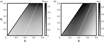
). Figure 4 presents (a)
 $C_{PGmax}$
and (b)
 $a_{max}$
as functions of
 $B_{l}$
and
 $B_{g}$
for the modelled array. Here,
 $C_{PGmax}$
refers to the maximum
 $C_{PG}$
for a given
 $B_{l}$
and
 $B_{g}$
. The tuned value of
 $a$
required to achieve
 $C_{PGmax}$
is referred to as
 $a_{max}$
. The thin white lines in the plots correspond to the optimal local blockage (
 $B_{l}^{opt}$
), which is the value of local blockage required for maximum power extraction at a given global blockage (
 $C_{PGmax}^{opt}$
). The value of
 $a_{max}$
at
 $B_{l}^{opt}$
is referred as
 $a_{max}^{opt}$
.
(a)
 $C_{PGmax}$
and (b)
 $a_{max}$
as functions of
 $B_{l}$
and
 $B_{g}$
for
 $Fr=0$
,
 $1/C_{f}=0$
and
 $L_{A/C}=0$
.
 $C_{PGmax}$
is the maximum global power coefficient for given values of
 $B_{l}$
and
 $B_{g}$
.
 $a_{max}$
is the tuned value of
 $a$
required to achieve
 $C_{PGmax}$
.

(a)
 $C_{PGmax}^{opt}$
, (b)
 $B_{l}^{opt}$
and
 $B_{ln}^{opt}$
and (c)
 $a_{max}^{opt}$
against
 $B_{g}$
for
 $Fr=0$
,
 $1/C_{f}=0$
and
 $L_{A/C}=0$
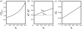
. It can be seen that the power extraction per turbine and the turbine resistance required to achieve it both increase with the global blockage, while the normalised optimal local blockage remains nearly unchanged.

Figure 5 shows the variation of (a)
 $C_{PGmax}^{opt}$
, (b)
 $B_{l}^{opt}$
and
 $B_{ln}^{opt}$
and (c)
 $a_{max}^{opt}$
against
 $B_{g}$
. Here,
 $B_{ln}=(B_{l}-B_{g})/(1-B_{g})$
is a normalised local blockage such that it varies from 0 to 1 when
 $B_{l}$
varies from
 $B_{g}$
to 1 and
 $B_{ln}^{opt}=(B_{l}^{opt}-B_{g})/(1-B_{g})$
. Figure 5(a) shows that
 $C_{PGmax}^{opt}$
increases with
 $B_{g}$
; this is because of the blockage effect which causes
 $C_{PG}$
to cross the Lanchester–Betz limit. A consequence of this phenomenon is that higher global blockage is desirable for increasing the power extraction per turbine. In addition, figure 5(b,c) shows that both
 $B_{l}^{opt}$
and
 $a_{max}^{opt}$
increase with increasing
 $B_{g}$
. This implies that more densely packed turbines with higher resistance are desirable in higher blockage cases.
The most important observation from these results is that the internal arrangement of turbines can be adjusted to an optimal value (
 $B_{l}^{opt}$
) to increase the power extraction per turbine. Nishino & Willden (Reference Nishino and Willden2012b
) explained this in terms of two competing effects. The first is that as the turbines are moved closer together, the increase in local blockage increases
 $\unicode[STIX]{x1D6FD}_{4L}$
and hence increases
 $C_{PG}$
. This is similar to the way in which the global blockage effect increases
 $\unicode[STIX]{x1D6FD}_{4A}$
and hence increases
 $C_{PG}$
. The second is that as the turbines are moved closer together, they start to block the flow through the array, i.e. the turbines cause a reduction in
 $\unicode[STIX]{x1D6FC}_{2A}$
, which decreases
 $C_{PG}$
. In between these two competing effects there is an optimum value of local blockage (
 $B_{l}^{opt}$
) which will give the maximum power extraction per turbine at a given global blockage (
 $C_{PGmax}^{opt}$
).
In this paper, we observe that this optimal local blockage, when normalised as
 $B_{ln}^{opt}$
, is a very weak function of
 $B_{g}$
as it remains almost constant at
 $B_{ln}^{opt}=0.37{-}0.39$
when
 $B_{g}$
is varied from 0.005 to 0.5. This means that regardless of the global blockage, the optimum local arrangement of turbines within the array remains the same. In other words, the optimal free area in a tidal array (
 $1-B_{l}^{opt}$
) is always approximately 60 % of the maximum free area allowed in the channel (
 $1-B_{g}$
). It is to be noted, however, that the existence of a nearly constant value of
 $B_{ln}^{opt}$
is true only in the present model in which there is no near-wake mixing (between
 $2L$
and
 $4L$
) regardless of the amount of shear created by the devices (i.e. the difference between
 $\unicode[STIX]{x1D6FD}_{4L}$
and
 $\unicode[STIX]{x1D6FC}_{4L}$
). This assumption will begin to break down in marine flows with high turbulence intensity.
3.2 The effect of surface deformation
When the flow passes through an array of turbines, they extract power from the flow. Consequently, the potential energy of the flow decreases downstream of the turbines. This reduction in the potential energy causes the water column height to drop, and this drop (or surface deformation) is proportional to the square of the Froude number as shown in (2.11). The effect of surface deformation is explored here by varying the Froude number of the incoming flow. The inherent channel drag coefficient is set to
 $1/C_{f}=0$
and the ratio of array length to channel length is set to
 $L_{A/C}=0$
to exclude the effect of added drag. Figure 6 shows the variation of (a)
 $C_{PGmax}^{opt}$
, (b)
 $B_{l}^{opt}$
and (c)
 $a_{max}^{opt}$
with
 $Fr$
, which is the Froude number of the undisturbed flow, for several values of
 $B_{g}$
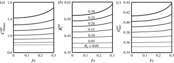
. Figure 6(a) shows that the surface deformation increases the power extraction per turbine. In addition, figures 6(b) and 6(c), respectively, show that the surface deformation also increases the local blockage and turbine resistance required to achieve the maximum power extraction per turbine.
Variation of (a)
 $C_{PGmax}^{opt}$
, (b)
 $B_{l}^{opt}$
and (c)
 $a_{max}^{opt}$
with
 $Fr$
and
 $B_{g}$
(
 $1/C_{f}=0$
and
 $L_{A/C}=0$
). The surface deformation, which is proportional to
 $Fr^{2}$
, increases the blockage effect slightly. Consequently, all three quantities increase slightly with
 $Fr$
.

The reason for this increase in
 $C_{PGmax}^{opt}$
,
 $B_{l}^{opt}$
and
 $a_{max}^{opt}$
with the surface deformation is that the drop in the water column height amplifies the blockage effect. The effect of surface deformation is higher with higher
 $B_{g}$
and the slope of variation is steeper with higher
 $Fr$
. For the case with the highest variation (
 $B_{g}=0.3$
), the changes in
 $B_{l}^{opt}$
and
 $a_{max}^{opt}$
associated with an increase in
 $Fr$
from 0 to 0.3 are approximately 10 % and 5 %, respectively.
In summary, like Whelan et al.’s (Reference Whelan, Graham and Peiró2009) model, this paper shows (i) that power extraction increases with Froude number and (ii) that higher turbine resistance is desirable in higher Froude number cases. We additionally show that a higher local blockage is desirable in the higher Froude number cases. All these changes, however, are small over the range of Froude numbers found in typical marine flows (
 $Fr\approx 0.1{-}0.2$
).
3.3 The effect of added drag from the installation of the tidal array
Figure 5(a) shows that the power extraction per turbine always increases when the fraction of the channel covered by turbines (
 $B_{g}$
) increases, and that the variation is faster than a linear variation. This, however, is not the case in realistic channels because of the effect of added drag from the array itself. The added drag decreases the incoming flow velocity (
 $U_{1d}$
), as shown in (2.7) and (2.16), and therefore has the effect of reducing the power extraction. As explained in § 2.3, the added drag comes from two sources – directly, from the drag imparted by turbines on the flow (
 $C_{TG}$
) and indirectly, from the tidal array-induced axial flow variations that increase the channel friction (
 $C_{fm}$
). The first term (
 $C_{TG}$
) is the main contributor to the added drag, and the second term (
 $C_{fm}$
) is relatively small and comes into play only when
 $L_{A/C}$
is large. When
 $L_{A/C}$
is large, a third effect comes into play: the friction force at the array scale (
 $C_{fm2}$
).
In order to investigate these effects, we fix the Froude number at
 $Fr=0.1$
and vary the value of
 $1/C_{f}$
from 0.15 to 0.95. The lower limit of
 $1/C_{f}$
as 0.15 is set to keep
 $\unicode[STIX]{x0394}H$
smaller than 0.05 (the model assumes that
 $\unicode[STIX]{x0394}H$
is small – § 2.1) and the upper limit is set as 0.95 to keep the seabed friction term (
 $f_{1}L_{c}/h_{1}$
) small. At first, we also set the channel length to be much higher than the array length (
 $L_{A/C}=0$
). This means that the effects of
 $C_{fm}$
and
 $C_{fm2}$
are both negligible. Figure 7 shows the variation of (a)
 $C_{PGmax}^{opt}$
, (b)
 $B_{l}^{opt}$
and (c)
 $a_{max}^{opt}$
with
 $1/C_{f}$
for several values of
 $B_{g}$
. The variation is more significant with higher
 $B_{g}$
and the slope of variation is steeper with smaller values of
 $1/C_{f}$
.
Variation of (a)
 $C_{PGmax}^{opt}$
, (b)
 $B_{l}^{opt}$
and (c)
 $a_{max}^{opt}$
with
 $1/C_{f}$
and
 $B_{g}$
for
 $Fr=0.1$
and
 $L_{A/C}=0$
. The effect of added drag from the turbines is small at
 $1/C_{f}=0.15$
and increases monotonically with
 $1/C_{f}$
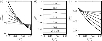
. It can be seen that both the power extraction and the turbine resistance required to achieve it reduce because of the effect of added drag. The optimal local blockage, however, is not affected by the effect of added drag when
 $L_{A/C}=0$
.

In the absence of the added drag effect (when
 $1/C_{f}$
is small), the blockage effect always increases the power extraction per turbine. Figure 7(a) shows that this blockage effect diminishes as
 $1/C_{f}$
increases. With higher values of
 $1/C_{f}$
, the advantage of increasing
 $B_{g}$
is partially nullified by the increase in the relative contribution of the turbines towards the total channel drag. Beyond a certain value of
 $1/C_{f}$
– approximately 0.8 for the channel modelled here – the power extraction per turbine actually starts to decrease with increasing
 $B_{g}$
.
Figure 7(b) shows that
 $B_{l}^{opt}$
is almost independent of
 $1/C_{f}$
, although there is a very small increase with increasing
 $1/C_{f}$
. Later we will see that this is true only when
 $L_{A/C}\approx 0$
. When the array length is comparable to the channel length then the size of the array (and hence
 $B_{l}$
) becomes important as explained in § 2.3, i.e. the effect of
 $C_{fm}$
and
 $C_{fm2}$
will change
 $B_{l}^{opt}$
. This finding could be inferred from the results in Garrett & Cummins (Reference Garrett and Cummins2013) where they show the effect of the size of a tidal array on power extraction.
Figure 7(c) shows that the optimal turbine resistance (
 $a_{max}^{opt}$
) decreases with increasing
 $1/C_{f}$
. This is because as
 $1/C_{f}$
increases, the contribution of turbines to the total channel drag is no longer negligible, and this additional drag therefore starts to reduce the power extracted by the array. It can also be seen that, at small values of
 $1/C_{f}$
, higher turbine resistance is desirable when the global blockage is higher. Beyond a certain value of
 $1/C_{f}$
– 0.3 for the channel modelled here – however,
 $a_{max}^{opt}$
actually decreases with increasing global blockage.
When the channel length is comparable to the array length, i.e.
 $L_{A/C}$
can no longer be taken to be approximately 0, the effects of
 $C_{fm}$
(added channel friction due to the array) and
 $C_{fm2}$
(friction at the array scale) come into play. The effects of both
 $C_{fm}$
and
 $C_{fm2}$
increase with friction (
 $C_{f}$
) and the length of the array (
 $L_{15A}$
), and for a given
 $L_{A/C}$
the length of the array increases with the local blockage (
 $B_{l}$
) as explained in § 2.3. On the one hand,
 $C_{fm}$
adds to the channel drag, which reduces the incoming flow velocity and hence adversely affects the power generation. Its effect, therefore, brings the optimal local blockage (
 $B_{l}^{opt}$
) to a lower value than that of the
 $L_{A/C}=0$
case. On the other hand,
 $C_{fm2}$
causes higher surface deformation at the array scale, which increases the flow through the turbines, and hence favourably affects the power generation. Its effect, therefore, brings the optimal local blockage (
 $B_{l}^{opt}$
) to a higher value than that of the
 $L_{A/C}=0$
case. The result of these two competing effects on
 $B_{l}^{opt}$
then depends upon whether the
 $C_{fm}$
or
 $C_{fm2}$
term dominates.
In order to investigate the effect of
 $C_{fm}$
and
 $C_{fm2}$
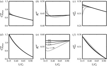
, figure 8 presents the variation of (a,d)
 $C_{PGmax}^{opt}$
, (b,e)
 $B_{l}^{opt}$
and (c,f)
 $a_{max}^{opt}$
with
 $1/C_{f}$
for various values of
 $L_{A/C}$
with
 $B_{g}=0.1$
(a–c) and
 $B_{g}=0.3$
(d–f). It can be seen from the trends in
 $B_{l}^{opt}$
in figures 8(b) and 8(e) that the effects of
 $C_{fm}$
and
 $C_{fm2}$
increase with decreasing
 $1/C_{f}$
and increasing
 $L_{A/C}$
. It can also be seen from figures 8(b) and 8(e) that
 $B_{l}^{opt}$
first decreases with decreasing
 $1/C_{f}$
(i.e. the effect of
 $C_{fm}$
is dominant in between
 $1/C_{f}=0.95$
and 0.3), and then increases if
 $1/C_{f}$
further reduces (i.e. the effect of
 $C_{fm2}$
is dominant in between
 $1/C_{f}\approx 0.3$
and 0.15).
Variation of (a,d)
 $C_{PGmax}^{opt}$
, (b,e)
 $B_{l}^{opt}$
and (c,f)
 $a_{max}^{opt}$
with
 $1/C_{f}$
and
 $L_{A/C}$
for
 $Fr=0.1$
and
 $B_{g}=0.1$
(a–c) and
 $B_{g}=0.3$
(d–f). Except at very small values of
 $1/C_{f}$
in the
 $B_{g}=0.1$
case,
 $B_{l}^{opt}$
decreases with
 $L_{A/C}$
. The effect of
 $L_{A/C}$
on
 $C_{PGmax}^{opt}$
and
 $a_{max}^{opt}$
is relatively small.

In the region where the effect of
 $C_{fm}$
is dominant (i.e.
 $1/C_{f}$
from 0.95 to approximately 0.3), it can be noted from figures 8(a,d) and 8(c,f) that the effect of
 $C_{fm}$
on
 $C_{PGmax}^{opt}$
and
 $a_{max}^{opt}$
, respectively, is relatively small. This is because the variation in both
 $C_{PGmax}^{opt}$
and
 $a_{max}^{opt}$
with
 $1/C_{f}$
is large because of the added drag effect from the turbines (
 $C_{TG}$
), as shown in figure 7. The slight changes caused by the effect of
 $C_{fm}$
are therefore negligible in this region. The effect of
 $C_{fm}$
, therefore, is important only in determining the optimal local blockage (
 $B_{l}^{opt}$
). Its effect is significant when
 $B_{g}$
is high, the channel length is short enough to be comparable to the array length (
 $L_{A/C}$
is close to 1), and the seabed friction coefficient is large (
 $1/C_{f}$
is small).
In the region where the effect of
 $C_{fm2}$
is dominant (i.e.
 $1/C_{f}$
from approximately 0.3 to 0.15), it can be noted from figures 8(b) and 8(e) that the effect of
 $C_{fm2}$
is much more pronounced in the
 $B_{g}=0.1$
case than in the
 $B_{g}=0.3$
case. This is because in the higher
 $B_{g}$
cases,
 $C_{fm}$
is relatively larger and partially nullifies the effect of
 $C_{fm2}$
; while in the lower
 $B_{g}$
cases,
 $C_{fm}$
is small. The steep increase in
 $B_{l}^{opt}$
between
 $1/C_{f}=0.15$
and 0.3 in the
 $B_{g}=0.1$
case also causes
 $C_{PGmax}^{opt}$
to increase (figure 8
a) and
 $a_{max}^{opt}$
to decrease (figure 8
c) noticeably. The effect of
 $C_{fm2}$
is important when
 $B_{g}$
is small, the channel length is short enough to be comparable to the array length (i.e.
 $L_{A/C}$
is close to 1 even at small
 $B_{g}$
), and the seabed friction coefficient is very large (i.e. large
 $C_{f}$
even when
 $L_{c}$
is small). This effect, therefore, is more likely to be important when turbines are arranged in multiple rows, where the array length could well be comparable to the channel length even when
 $B_{g}$
is small.
In summary, the effect of added drag is crucial in determining the turbine resistance required to maximise
 $C_{PG}$
. A model which neglects the turbine drag will over-predict the induction factor required to maximise the power extracted (see figure 7
c). Moreover, the added drag has to be considered in order to estimate the optimum global blockage correctly, i.e. the fraction of the channel area that should be occupied by turbines for maximum power extraction per turbine (see figure 7
a). The installation of a tidal array causes a further increase in the channel friction by creating cross-stream variations in the axial velocity, and this effect leads to a lower optimal local blockage than would otherwise be expected (see figure 8
b,e). This is true except when the effect of friction at the array scale becomes important, i.e. very large
 $C_{f}$
,
 $L_{A/C}\approx 1$
and small
 $B_{g}$
. In such cases, a much higher optimal local blockage is desirable than in the case where
 $L_{A/C}$
is negligible (see figure 8
b). The effect of seabed friction at the array scale also reduces the optimal turbine induction factor (see figure 8
c).
4 Discussion
As explained in § 1, it is the consideration of the effects of local blockage, surface deformation and added drag from the tidal array simultaneously in one model that sets our model apart from those in the literature. The individual effects are discussed in § 3, and are comparable to those given by the previously verified models of Whelan et al. (Reference Whelan, Graham and Peiró2009), Vennell (Reference Vennell2010) and Nishino & Willden (Reference Nishino and Willden2013). In this section, we focus on the importance of considering the various effects simultaneously before discussing the limitations of the present model and suggesting potential improvements.
4.1 Combined effect
Nishino & Willden’s (Reference Nishino and Willden2013) model shows that the local blockage in a tidal array can be adjusted to optimise the power extraction per turbine. Their model can, therefore, be used to obtain the optimum local blockage (
 $B_{l}^{opt}$
) and the corresponding optimum turbine resistance (
 $a_{max}^{opt}$
) in a tidal array. A major limitation in their model, however, is that they ignore the channel parameters, including the Froude number and the channel drag coefficient. Such a model, therefore, cannot account for the effects of surface deformation or of the added drag from the tidal array.
The model presented in this paper has shown that the surface deformation effect is small, but that the added drag effect can be significant. We have shown that neglecting the added drag can give significantly higher values of turbine tuning and slightly higher local blockage than that required to achieve the optimum performance (see figures 7
c and 8
b,e). We have also shown that when the channel length is short enough to be comparable to the array length, then the effect of friction at the array scale also comes into play. In some extreme cases, when
 $C_{f}$
is very large,
 $L_{A/C}$
is close to 1, and
 $B_{g}$
is small (i.e. very high channel friction coefficient
 $f_{1}$
), this effect leads to a sharp increase in the optimal local blockage (see figure 8
b) and a decrease in the optimal turbine resistance (see figure 8
c). As mentioned before, this effect is more likely to be important when multiple rows are considered and hence the array length is large even when
 $B_{g}$
is small.
More importantly, because Nishino & Willden’s (Reference Nishino and Willden2013) model does not account for the added drag effect, it gives a monotonic increase in power extraction per turbine with global blockage. Consequently, it cannot be used to predict up to what limit a channel should be occupied by turbines for maximum power extraction per turbine. In the present model, we include the effect of added drag caused by the installation of a tidal array in a channel. This effect of added drag is more pronounced in channels with lower inherent drag, i.e. in channels with higher
 $1/C_{f}$
values. It was shown in figure 7(a) that
 $C_{PGmax}^{opt}$
decreases with increasing
 $1/C_{f}$
. This decrease is more marked in cases with higher global blockage. Consequently, beyond
 $1/C_{f}=0.8$
in the present model,
 $C_{PGmax}^{opt}$
starts to decrease with
 $B_{g}$
.
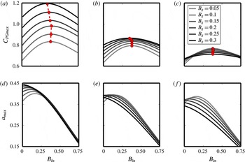
In order to investigate the combined effect of the local blockage and added drag, figure 9(a–c) shows the variation of
 $C_{PGmax}$
with
 $B_{ln}$
and
 $B_{g}$
for
 $1/C_{f}=0.15$
, 0.50 and 0.80, respectively, at
 $Fr=0.1$
and for a channel such that
 $L_{A/C}=1$
when
 $B_{g}=0.3$
(i.e.
 $L_{A/C}=1/6$
when
 $B_{g}=0.05$
,
 $L_{A/C}=1/3$
when
 $B_{g}=0.1$
, and so on for the other
 $B_{g}$
values using the linear relationship explained in § 2.3). These plots show that the optimum global blockage, i.e. the value of
 $B_{g}$
at which the power extraction per turbine is maximised, is determined by the combined effect of the added drag and the local blockage. The optimum global blockages required in the three cases are (a)
 $B_{g}\approx 1.00$
, (b)
 $B_{g}\approx 0.55$
(results not shown here for such high
 $B_{g}$
values) and (c)
 $B_{g}<0.05$
. If the effect of added drag alone is considered without exploring the effect of local blockage, as in the model given by Vennell (Reference Vennell2010), then the resultant optimum
 $B_{g}$
would be much higher. Those results will correspond to
 $B_{ln}=0$
in these plots, for which the optimum
 $B_{g}$
in the three cases are (a)
 $B_{g}=1.00$
, (b)
 $B_{g}=1.00$
and (c)
 $B_{g}\approx 0.25$
.
The dots in the plots show the optimal local blockage required for
 $C_{PGmax}^{opt}$
. It can be seen that
 $B_{ln}^{opt}$
decreases with
 $B_{g}$
instead of slightly increasing as was shown in figure 5, when the effect of local blockage was considered in isolation. This reduction in
 $B_{ln}^{opt}$
with
 $B_{g}$
is because of the effect of the tidal array-induced increase in channel friction (
 $C_{fm}$
).
Variation of (a–c)
 $C_{PGmax}$
and (d–f)
 $a_{max}$
against
 $B_{ln}$
and
 $B_{g}$
at
 $Fr=0.1$
and (a,d)
 $1/C_{f}=0.15$
, (b,e)
 $1/C_{f}=0.5$
and (c,f)
 $1/C_{f}=0.8$
for the channel length such that
 $L_{A/C}=1$
when
 $B_{g}=0.3$
. Vennell’s (Reference Vennell2010) model is approximately equivalent to
 $B_{ln}=0$
, i.e.
 $B_{l}=B_{g}$
.

Figure 9(d–f) shows the variation of
 $a_{max}$
with
 $B_{ln}$
for different values of
 $1/C_{f}$
(with the same values of
 $B_{g}$
,
 $1/C_{f}$
and
 $L_{A/C}$
as in figure 9(a–c)). These plots show that for any global blockage value, the turbine tuning (
 $a_{max}$
) required to achieve
 $C_{PGmax}$
is always lower at the optimum local blockage (
 $B_{ln}\approx 0.38$
) than at
 $B_{ln}=0$
. To understand the significance of this result, consider that the power wasted by the array is the difference between the power extracted by the array (
 $P_{A}=T_{A}U_{1d}\unicode[STIX]{x1D6FC}_{2A}$
) and the power extracted by the turbines (
 $nP_{D}=nT_{d}U_{1d}\unicode[STIX]{x1D6FC}_{2A}\unicode[STIX]{x1D6FC}_{2L}=T_{A}U_{1d}\unicode[STIX]{x1D6FC}_{2A}\unicode[STIX]{x1D6FC}_{2L}$
). The relative power wastage, therefore is
 $(P_{A}-nP_{D})/P_{A}=1-\unicode[STIX]{x1D6FC}_{2L}$
, which is approximately equal to the value of
 $a$
(
 $1-\unicode[STIX]{x1D6FC}_{2L}/m_{1}k_{1}$
). This means that exploring the local blockage effect not only increases the power extraction per turbine but also reduces the proportion of the power wasted by the array arrangement.
In summary, figure 9 shows that considering the added drag alone and not exploring the effect of local blockage leads to over-predictions of both the global blockage (
 $B_{g}$
) and the turbine resistance (
 $a$
) for maximum power extraction per turbine. Figure 9(a–c) shows that the value of
 $B_{g}$
for optimum
 $C_{PGmax}$
is higher at
 $B_{ln}=0$
than at
 $B_{lnopt}$
(i.e. at
 $B_{ln}\approx 0.38$
). Similarly, figure 9(d–f) shows that the value of
 $a_{max}$
required to achieve
 $C_{PGmax}$
is also higher at
 $B_{ln}=0$
than at
 $B_{lnopt}$
. We have already seen from figure 7 that not considering the effect of added drag, i.e. assuming large
 $C_{f}$
or small
 $1/C_{f}$
, also leads to a higher value of
 $a$
than that required for maximum power extraction per turbine and shows, incorrectly, a monotonic increase in
 $C_{PG}$
with
 $B_{g}$
. This means that ignoring either of the two effects – added drag or local blockage – leads to higher
 $B_{g}$
and
 $a$
than the optimum, which in turn leads to unnecessary addition of extra turbines and higher power wastage.
Surface deformation effects are not considered in this section and the Froude number is kept fixed at 0.1. This is because the surface deformation effects are small over the range of Froude numbers applicable to most tidal energy sites (
 $Fr=0.1-0.2$
). Moreover, the surface deformation effect simply means that slightly higher
 $B_{g}$
,
 $B_{l}$
, and
 $a$
values are required for optimal performance in higher Froude number cases. This means that Froude number can be considered independently of the other parameters without any adverse effect on the optimised array design.
4.2 Model limitations and future improvements
Although our model considers the above mentioned three effects simultaneously, there are a number of other effects that are not considered here. The main limitation of our model is that we have ignored the effect of several flow parameters, such as Reynolds number, turbulence intensity and velocity and density profiles. Further to this, our turbine tuning parameter does not capture the complexity of a real turbine’s operations. There is, for example, no consideration of the swirl imparted on the flow by each turbine. These flow parameters and the amount of swirl in the flow will have a major impact on the wake mixing process.
Wake mixing plays an important role in the functioning of turbines – Reynolds-averaged Navier–Stokes (RANS) simulations undertaken by Nishino & Willden (Reference Nishino and Willden2012a
) showed that mixing increased the power extraction. To understand its role, consider that as the turbines come closer together, our model predicts that the speed of the local bypass flow between the turbines increases relative to that of the local core flow. This local blockage effect then increases the power extraction by the turbines. The creation of this velocity difference in the flow at the turbine location is dependent upon the wake mixing in the downstream region. In the present model (as in Nishino & Willden’s (Reference Nishino and Willden2013) model) it is assumed that (i) there is no near-wake mixing (between locations
 $2L$
and
 $4L$
) and (ii) the far-wake mixing is completed before location
 $4A$
regardless of the amount of velocity difference created at the turbine location.
These assumptions are not completely satisfied in a real flow. Additionally, as mentioned in § 2.2, the array-scale and device-scale vertical mixing processes are likely to happen in the same region rather than separately as assumed in the present model. Nishino & Willden (Reference Nishino and Willden2013) also found that many of the discrepancies between their model and RANS simulations are caused by discrepancies in the wake mixing. Further work is therefore required to understand how different flow features affect the wake mixing process and hence the power extraction by the turbines.
Turbines are modelled as porous discs in the present model. They, however, are far more complex in reality. The most important difference is that a real turbine consists of blades which rotate such that the flow at the upstream face has a higher pressure than the flow at the downstream face of the blades. This pressure difference, which creates the power, depends up on the lift and drag coefficients of the blades. The lift and drag coefficients, in turn, depend upon the blade angle of attack, which is found from the relative magnitudes of the upstream flow velocity and the turbine rotational speed. The lift and drag coefficients will also be strongly dependent on the flow Reynolds number. One way to include these effects would be via empirical models for the effect of different flow parameters on turbine performance based on available data from numerical simulations or experimental results.
For the sake of brevity, other effects neglected in the present model are flow acceleration and drag from the support structures. The flow acceleration term arises from the time dependence of the tides and is included in Garrett & Cummins (Reference Garrett and Cummins2005). We have assumed that the time scale of the variation of the tide is much larger than the time it takes the flow to pass through the channel. Consequently, a quasi-steady approximation is valid. This time acceleration term could be added to the momentum equations (2.3) and (2.5), where it would have the same effect as channel bottom friction. Including it would, therefore, not lead to a qualitative change in the results presented in this paper. It should be noted, however, that unlike Vennell (Reference Vennell2016), we do not consider the maximisation of tidal energy generation over a tidal cycle, where the variation in tidal head with time should be considered. The drag from support structures also increases the friction in channel, similar to the flow acceleration explained above. This term can cause significant power loss in channels with several rows of turbines as shown in Vennell (Reference Vennell2012).
Lastly, we have not considered the optimisation of an array with several rows of turbines placed downstream of one another. This is partially done in Draper & Nishino (Reference Draper and Nishino2013), who show the complexity of this issue as many combinations of row arrangement are possible. This shows the significance of an automated way of optimising turbine arrangement, such as the method of Funke et al. (Reference Funke, Farrell and Piggott2014), in place of manual methods for arranging the turbines.
5 Conclusions
A major challenge to the commercial extraction of tidal energy is the cost of power generation. One of the ways to bring the cost down is to optimise tidal arrays for maximum power extraction per turbine. There are several factors which affect the power extraction of turbines in an array. Some of the key factors are: inherent friction in the channel, the resistance of turbines, the intra-turbine spacing in the array, the number of rows of turbines and the wake mixing caused by turbulence and swirl. There are several models in the literature that account for one or more of those key factors and show their influence on the performance of tidal arrays. However, different effects are typically considered in isolation.
In this paper, we have developed an analytical model that simultaneously considers the effects of (i) the local blockage, (ii) the free surface deformation and (iii) the added drag due to the tidal array. We show that exploring the effect of local blockage (by adjusting
 $B_{l}$
) can significantly increase the power extraction per turbine. We find that the surface deformation effect, which is higher at higher Froude numbers, leads to the requirement of slightly higher turbine resistance and slightly more closely packed turbines to achieve the maximum possible power extraction per turbine. We find that the effect of added drag, which is higher in channels with smaller inherent drag coefficient (
 $C_{f}$
), partially or completely nullifies the supposed advantage of increasing the global blockage
 $B_{g}$
. The effect of added drag is found to be crucial in determining the turbine resistance required to achieve maximum
 $C_{PG}$
and also reduces the optimal local blockage (
 $B_{l}^{opt}$
) slightly. In very short channels with very high seabed friction coefficient, the effect of the friction at the array scale is also found to be important. It increases the optimal local blockage and decreases the optimal turbine resistance noticeably.
Most importantly, we find that the effects of local blockage and added drag must be considered simultaneously in order to determine the optimal channel blockage and the required turbine resistance for a tidal array with maximum power extraction per turbine. In isolation, both effects will lead to over-estimates of both the global blockage and the turbine resistance required for optimum array design. We, therefore, conclude that considering one of the two effects alone will lead to the addition of unnecessary turbines and the higher wastage of power through dissipation.
Finally, the importance has been shown of including all the factors that affect the power extraction of an array in one model. This is because the optimal design is a result of an interplay between different effects. The present model includes three important effects: the local blockage, the added drag due to the tidal array and the surface deformation. In future, the influence of other factors, such as the flow Reynolds number, turbulence intensity, velocity and density profiles as well as the swirling flow imparted by the turbines, should be analysed and those factors that are found to be important should be incorporated along with the three factors already present in the model here.
Acknowledgements
The authors wish to thank R. Willden, T. Nishino, C. Vogel and others for the very helpful discussions at the Oxford Tidal Energy workshop. The work was mainly funded by the Newton Fund through EPSRC, UK (EP/M019896/1). The first author was supported by NSFC, China (grant no. 11672123) during the later stages of this research.
Appendix A. Final set of equations
The final set of 12 equations are given below in terms of 12 unknown variables (
 $U_{1nd}$
,
 $C_{TG}$
,
 $\unicode[STIX]{x1D6FC}_{c}$
,
 $\unicode[STIX]{x1D6FC}_{2A}$
,
 $\unicode[STIX]{x1D6FC}_{4A}$
,
 $\unicode[STIX]{x1D6FD}_{4A}$
,
 $H_{4}$
,
 $\unicode[STIX]{x1D6FC}_{2L}$
,
 $\unicode[STIX]{x1D6FC}_{4L}$
,
 $\unicode[STIX]{x1D6FD}_{4L}$
,
 $m_{1}k_{1}$
and
 $m_{4}k_{4}$
), five design parameters (
 $B_{g}$
,
 $B_{a}$
,
 $B_{l}$
,
 $n$
and
 $a$
) and three channel parameters (
 $C_{f}$
,
 $L_{c}$
and
 $Fr$
). These equations are numerically solved in Python using a Newton–Raphson method.
 $$\begin{eqnarray}\displaystyle & \displaystyle \unicode[STIX]{x1D6FC}_{c}B_{a}+0.5(\unicode[STIX]{x1D6FD}_{4A}+1)(1-B_{a})=1, & \displaystyle\end{eqnarray}$$
 $$\begin{eqnarray}\displaystyle & \displaystyle U_{1nd}^{2}=\frac{C_{f}}{C_{f}+C_{fm}}-\frac{C_{TG}B_{g}}{C_{f}+C_{fm}}, & \displaystyle\end{eqnarray}$$
 $$\begin{eqnarray}\displaystyle & \displaystyle \unicode[STIX]{x1D6FD}_{4A}\left(H_{4}-B_{a}\frac{\unicode[STIX]{x1D6FC}_{2A}}{\unicode[STIX]{x1D6FC}_{4A}}\right)=1-\unicode[STIX]{x1D6FC}_{2A}B_{a}, & \displaystyle\end{eqnarray}$$
 $$\begin{eqnarray}\displaystyle & \displaystyle B_{l}C_{TG}=U_{1nd}^{2}(\unicode[STIX]{x1D6FD}_{4A}^{2}-\unicode[STIX]{x1D6FC}_{4A}^{2}), & \displaystyle\end{eqnarray}$$
 $$\begin{eqnarray}\displaystyle & \displaystyle H_{4}=1-\frac{Fr^{2}}{2}U_{1nd}^{2}[(\unicode[STIX]{x1D6FD}_{4A}^{2}-1)+C_{fm2}], & \displaystyle\end{eqnarray}$$
 $$\begin{eqnarray}\displaystyle & \displaystyle 2U_{1nd}^{2}[1-\unicode[STIX]{x1D6FD}_{4A}+\unicode[STIX]{x1D6FC}_{2A}B_{a}(\unicode[STIX]{x1D6FD}_{4A}-\unicode[STIX]{x1D6FC}_{4A})]=C_{TG}B_{g}+U_{1nd}^{2}C_{fm2}-\frac{1}{Fr^{2}}(1-H_{4}^{2}), & \displaystyle\end{eqnarray}$$
 $$\begin{eqnarray}\displaystyle & \displaystyle \unicode[STIX]{x1D6FD}_{4L}=\frac{1-\unicode[STIX]{x1D6FC}_{2L}B_{l}}{1-{\displaystyle \frac{\unicode[STIX]{x1D6FC}_{2L}}{\unicode[STIX]{x1D6FC}_{4L}}}B_{l}}, & \displaystyle\end{eqnarray}$$
 $$\begin{eqnarray}\displaystyle & \displaystyle C_{TG}=U_{1nd}^{2}\unicode[STIX]{x1D6FC}_{2A}^{2}(m_{4}k_{4})^{2}[\unicode[STIX]{x1D6FD}_{4L}^{2}-\unicode[STIX]{x1D6FC}_{4L}^{2}], & \displaystyle\end{eqnarray}$$
 $$\begin{eqnarray}\displaystyle \frac{(m_{4}k_{4})^{2}}{2}(\unicode[STIX]{x1D6FD}_{4L}^{2}-\unicode[STIX]{x1D6FC}_{4L}^{2}) & = & \displaystyle \frac{m_{1}k_{1}}{B_{l}}-m_{4}k_{4}\unicode[STIX]{x1D6FC}_{4L}\unicode[STIX]{x1D6FC}_{2L}-\frac{m_{4}k_{4}\unicode[STIX]{x1D6FD}_{4L}^{2}}{B_{l}}+m_{4}k_{4}\unicode[STIX]{x1D6FD}_{4L}^{2}\frac{\unicode[STIX]{x1D6FC}_{2L}}{\unicode[STIX]{x1D6FC}_{4L}}\nonumber\\ \displaystyle & & \displaystyle +\,\frac{1}{2B_{l}m_{4}k_{4}}[(m_{4}k_{4}\unicode[STIX]{x1D6FD}_{4L})^{2}-(m_{1}k_{1})^{2}],\end{eqnarray}$$
 $$\begin{eqnarray}\displaystyle & \displaystyle \unicode[STIX]{x1D6FC}_{2L}=m_{1}k_{1}(1-a), & \displaystyle\end{eqnarray}$$
 $$\begin{eqnarray}\displaystyle & \displaystyle m_{1}k_{1}=\left[1+\left(\frac{1}{n}\right)(\unicode[STIX]{x1D6FC}_{2A}-1)\right]^{-1}, & \displaystyle\end{eqnarray}$$
 $$\begin{eqnarray}\displaystyle & \displaystyle m_{4}k_{4}=\left[1+\left(\frac{1}{n}\right)\left(\frac{\unicode[STIX]{x1D6FC}_{2A}}{\unicode[STIX]{x1D6FC}_{4A}}-1\right)\right]^{-1}. & \displaystyle\end{eqnarray}$$
Where
 $C_{fm}=(2f_{1}L_{15A}/h_{1})(B_{a}\unicode[STIX]{x1D6FC}_{c}^{2}+(1-B_{a})((1+\unicode[STIX]{x1D6FD}_{4A})/2)^{2}-1)$
and
 $C_{fm2}=(2f_{1}L_{14A}/h_{1})(B_{a}\unicode[STIX]{x1D6FC}_{c}^{2}+(1-B_{a})((1+\unicode[STIX]{x1D6FD}_{4A})/2)^{2})$
are friction terms due to the array-induced axial flow speed variations and drag at the array scale, respectively.
The length parameters are
 $L_{14A}=0.7L_{15A}$
and
 $L_{15A}=L_{Array}(((n-1)B_{l}+1)/n)$
and
 $L_{Array}$
is linearly proportional to
 $B_{g}$
in a given channel.