

1. Introduction
Bubbles transported by turbulent flows in nature and industrial applications are constantly deformed by the surrounding turbulent stresses. The question of how the deformation affects the bubble's orientation and translational motion constitutes one of the fundamental and practically important two-phase flow problems. Significant effort has been devoted to simpler rigid particles, including both spherical (Balachandar & Eaton Reference Balachandar and Eaton2010) and non-spherical particles (Voth & Soldati Reference Voth and Soldati2017), which has helped to advance both the physical understanding of turbulent two-phase flows and different numerical and experimental techniques. Adding particle deformation to these already complicated problems introduces new challenges and opportunities.
One challenge is related to the deformation and orientation dynamics of deformable bubbles/drops, which are crucial to their experienced hydrodynamic forces. For instance, the added mass (Lamb Reference Lamb1924; Brennen Reference Brennen1982, Reference Brennen2005; Magnaudet & Eames Reference Magnaudet and Eames2000), lift (Mathai, Lohse & Sun Reference Mathai, Lohse and Sun2020) and drag all depend on the relative orientation of the bubbles with their surrounding flows and on the bubble aspect ratio. The direct numerical simulation has made significant progress in addressing this problem (Elghobashi Reference Elghobashi2019); however, it is often quite expensive to resolve the complex deformation of finite-sized bubbles/droplets in turbulence. As a result, only the deformation of small, sub-Kolmogorov-scale, neutrally buoyant droplets has been studied using phenomenological models (Maffettone & Minale Reference Maffettone and Minale1998; Biferale, Meneveau & Verzicco Reference Biferale, Meneveau and Verzicco2014). However, most deformable bubbles in turbulence are much larger and likely to be in the inertial range. In this paper, our focus is on finite-sized deformable bubbles with volume-equivalent sphere diameter ( $D$) in the inertial range (
 $\eta \ll D\ll L$), where
 $\eta$ is the Kolmogorov scale and
 $L$ is the integral length scale. Therefore, their deformation is driven by the gradient of dynamic pressure acting on the bubble interface, rather than by viscous stresses.
Most prior investigations on the orientation of deformable bubbles are limited to simple flow configurations, e.g. viscous shear flows (in which the orientation of bubbles was measured as a function of the capillary number), size (Rust & Manga Reference Rust and Manga2002; Kameda, Katsumata & Ichihara Reference Kameda, Katsumata and Ichihara2008), or the viscosity ratio (Müller-Fischer et al. Reference Müller-Fischer, Tobler, Dressler, Fischer and Windhab2008). In these cases, the flows were in a quasi-steady state, and the flow inertia could be neglected. A final steady state for the bubble orientation that solely depends on the balance between the flow shear and the capillary stress hence can be reached (Huber et al. Reference Huber, Su, Nguyen, Parmigiani, Gonnermann and Dufek2014). Furthermore, significant attention has been paid to the deformation and orientation of oil droplets in steady shear flows (Guido & Greco Reference Guido and Greco2001; Megías-Alguacil, Fischer & Windhab Reference Megías-Alguacil, Fischer and Windhab2006; Feigl et al. Reference Feigl, Megias-Alguacil, Fischer and Windhab2007; Armandoost, Bayareh & Nadooshan Reference Armandoost, Bayareh and Nadooshan2018).
The study of bubbles/droplets deformed by viscous flows has also been extended to turbulence, although limited solely to sub-Kolmogorov-scale neutrally buoyant droplets, because droplets at this scale remain subject to viscous deformation even in turbulence. For this problem, the background turbulence is simulated first, and the orientation and deformation of droplets can be calculated by employing the same phenomenological model used by Maffettone & Minale (Reference Maffettone and Minale1998); inputs being the local turbulent vorticity and strain rates (Biferale et al. Reference Biferale, Meneveau and Verzicco2014). In this work, unlike small rigid non-spherical particles, e.g. rods and fibres (Shin & Koch Reference Shin and Koch2005; Parsa et al. Reference Parsa, Calzavarini, Toschi and Voth2012; Chevillard & Meneveau Reference Chevillard and Meneveau2013; Ni et al. Reference Ni, Kramel, Ouellette and Voth2015), the semi-major axis of the deformed droplets show stronger alignment with the maximum stretching direction of turbulent strain rate than with the vorticity vector, but the degree of this alignment decreases with an increasing capillary number. A similar method was also applied to sub-Kolmogorov neutrally buoyant droplets (Spandan, Lohse & Verzicco Reference Spandan, Lohse and Verzicco2016) and bubbles (Spandan, Verzicco & Lohse Reference Spandan, Verzicco and Lohse2017) in turbulent Taylor–Couette flows. The semi-major axis of these droplets also preferentially aligns with the maximum stretching direction, with a stronger alignment near the wall than in bulk region where the flow is more isotropic.
Finite-sized bubbles deforming in intense turbulence are in the opposite limit, where the viscous effect becomes negligible (the capillary number is much smaller than one). Owing to the limited studies in this regime, we examine another case of a bubble rising in an otherwise quiescent medium following a non-rectilinear path, where the bubble is deformed by the pressure gradient induced by buoyancy, and the bubble-size-based Reynolds number is sufficiently large. The semi-minor axis of the bubble typically aligns with its velocity (Lunde & Perkins Reference Lunde and Perkins1998; Ellingsen & Risso Reference Ellingsen and Risso2001; Riboux, Risso & Legendre Reference Riboux, Risso and Legendre2010; Legendre, Zenit & Velez-Cordero Reference Legendre, Zenit and Velez-Cordero2012) within less than  $2^\circ$ (Mougin & Magnaudet Reference Mougin and Magnaudet2001; Ern et al. Reference Ern, Risso, Fabre and Magnaudet2012), whereas both directions oscillate about the vertical axis within
 $30^{\circ }$ (Riboux et al. Reference Riboux, Risso and Legendre2010; Ellingsen & Risso Reference Ellingsen and Risso2001; Ern et al. Reference Ern, Risso, Fabre and Magnaudet2012) for a wide range of bubble sizes (Luewisutthichat, Tsutsumi & Yoshida Reference Luewisutthichat, Tsutsumi and Yoshida1997). For this regime, the orientational dynamics are therefore periodic, and the oscillation of the bubble orientation is more closely related to its wake oscillation rather than to its deformation (Tayler et al. Reference Tayler, Holland, Sederman and Gladden2012).
In high-Reynolds-number turbulent flows, bubbles were also observed to oscillate periodically within around  $45^{\circ }$ about the vertical axis (Ravelet, Colin & Risso Reference Ravelet, Colin and Risso2011), which is consistent with that reported in a quiescent medium but with a slightly larger amplitude. One plausible explanation for such a similar bubble behaviour in both quiescent and turbulent media is that, in the experiment by Ravelet et al. (Reference Ravelet, Colin and Risso2011), turbulence was relatively weak compared with buoyancy. As a result, bubbles were still preferentially deformed by buoyancy, thereby aligning with the vertical direction. If the pressure gradient induced by turbulent stresses is stronger than that due to buoyancy, new phenomena may emerge. A recent work showed that finite-sized bubbles rising in intense turbulence experience different lift and drag forces due to the turbulence-induced deformation (Salibindla et al. Reference Salibindla, Masuk, Tan and Ni2020).
In the current study, we experimentally measure the bubble orientational dynamics in intense turbulence, where turbulent stresses become more important than buoyancy. The three-dimensional (3-D) shape and surrounding turbulent flows are measured simultaneously. The experimental set-up and measurement techniques used are introduced in § 2.1, whereas the measurable quantities and their calculations are summarized in § 2.2. The acquired unique data set helps us to investigate the preferential alignment of the bubble semi-major ( $\hat {{\boldsymbol {r}}}_1$) and semi-minor axes (
 $\hat {{\boldsymbol {r}}}_3$) with the representative directions of two deformation mechanisms, i.e. the slip velocity and turbulent strain rate, which are discussed in § 3.1. Finally, the evolution of the relative orientation of the bubble with the surrounding turbulence as it approaches the moment of breakup is introduced and explained in § 3.2.
2. Experimental set-up and measurements
2.1. Experimental set-up
In this study, a vertical water tunnel named V-ONSET was utilized to measure the interaction between deforming air bubbles and surrounding turbulence. V-ONSET was designed to generate intense turbulence with a large mean energy dissipation rate  $\langle \epsilon \rangle$ of
 $O(0.1)\ \textrm {m}^{2}\ \textrm {s}^{-3}$ while maintaining a nearly homogeneous and isotropic environment over a measurement volume of
 $6\ \textrm {cm}\times 6\ \textrm {cm}\times 5\ \textrm {cm}$. At this
 $\langle \epsilon \rangle$, the Kolmogorov length and time scales were determined to be
 $\eta \approx 50\ \mathrm {\mu }\textrm {m}$ and
 $\tau _\eta \approx 2.5\ \textrm {ms}$, respectively. Key facility features are briefly summarized below. Additional details concerning the experimental rig and its flow characteristics can be found in Masuk et al. (Reference Masuk, Salibindla, Tan and Ni2019b).
In the test section of V-ONSET, intense turbulence was generated by firing high-speed momentum jets (up to  $12\ \textrm {m}\ \textrm {s}^{-1}$) into the test section through randomly selected nozzles (the nozzle diameter
 $d$ is 5 mm) from a jet array. On average, 12.5 % of the total 88 jets were kept activated since this was found to maximize the turbulence intensity, and their firing pattern was randomized following a Gaussian distribution. This firing scheme follows the work by Variano, Bodenschatz & Cowen (Reference Variano, Bodenschatz and Cowen2004), to ensure that no secondary flow structure would develop in the test section (De Silva & Fernando Reference De Silva and Fernando1994; Srdic, Fernando & Montenegro Reference Srdic, Fernando and Montenegro1996; Variano et al. Reference Variano, Bodenschatz and Cowen2004). The jet array was located approximately 80
 $d$ above the measurement location to allow jets to be fully mixed before reaching the interrogation volume. In addition, a uniform downward mean flow, with magnitude similar to the bubble rise velocity, was introduced to keep bubbles within the measurement volume for an extended time. Moreover, bubbles were generated through four groups of hypodermic needles of two sizes, which are located at the bottom of the test section. Once a bubble reached the test section, its 3-D shape was reconstructed from the virtual-camera visual-hull method (Masuk, Salibindla & Ni Reference Masuk, Salibindla and Ni2019a). The probability density function (p.d.f.) of the volume-equivalent sphere size
 $D$ of the bubbles is shown in figure 1. The typical bubble size range in the test section is approximately 2–7 mm in diameter, with most around 3–4 mm.
The distribution of the volume-equivalent sphere diameter  $D$ of all bubbles in our experiments.

Six high-speed cameras were distributed all around the tunnel's octagonal test section to simultaneously acquire images of both phases from different directions. Six LED panels, one for each camera, were used to provide diffused back-lighting, which results in a white background. The dark silhouettes of large dispersed bubbles and tracer particles can be identified, segmented and eventually separated based on their contrasts from the background and their size differences (the diameter of the tracer particle is  $50 \ \mathrm {\mu }\textrm {m}$). After image segmentation, large bubble silhouettes were input into the 3-D shape reconstruction method, whereas the tracer locations were tracked using our in-house Shake-The-Box method (Schanz, Gesemann & Schröder Reference Schanz, Gesemann and Schröder2016; Tan et al. Reference Tan, Salibindla, Masuk and Ni2020) (the code is available online @JHU-Ni-Lab on GitHub). Flow information, such as velocity and acceleration, can be calculated from these 3-D trajectories. A high concentration of tracer particles could potentially contaminate the bubble interface and modulate its boundary condition; however, this effect is less important for finite-sized bubbles because their deformation is primarily driven by inertia (or, more specifically, the gradient of dynamic pressure) rather than by viscous stresses. Therefore, the contamination is not expected to affect the deformation statistics reported in this paper.
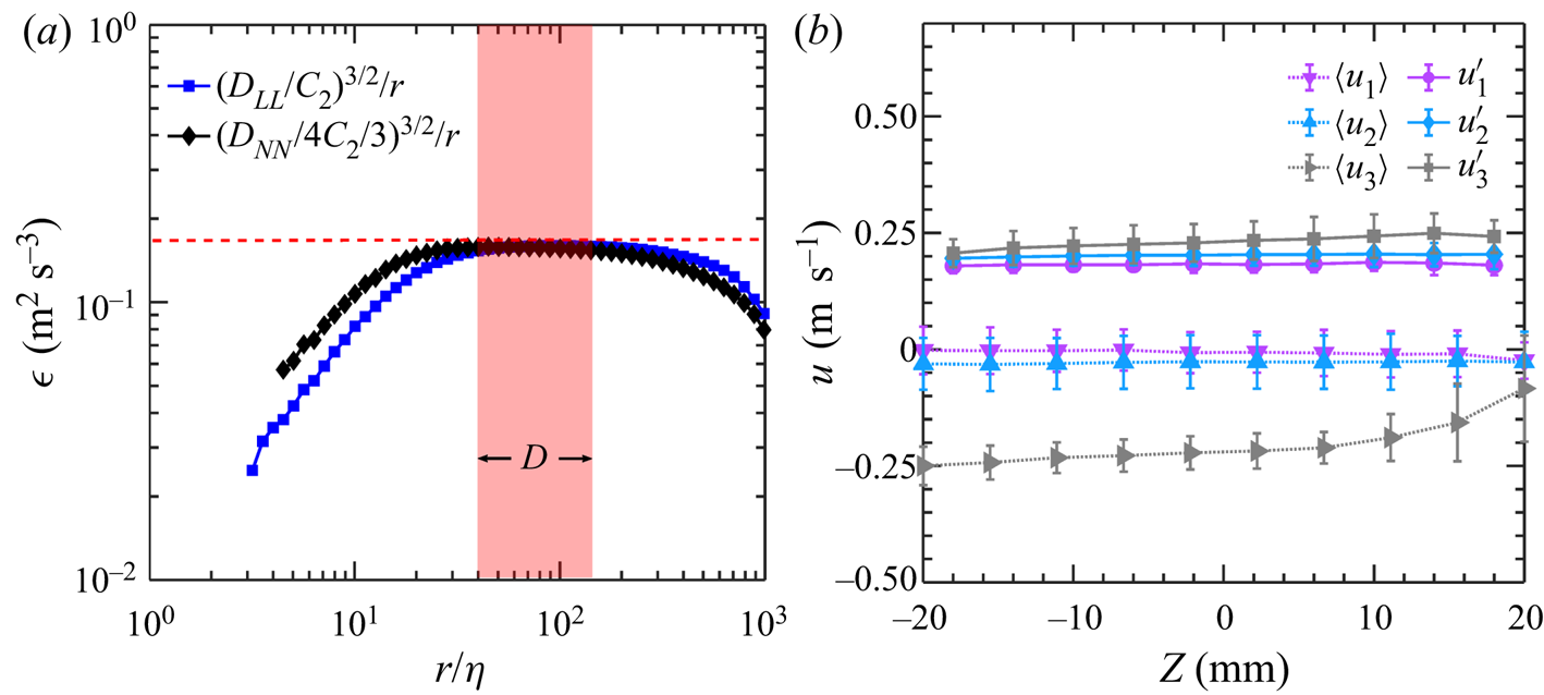
To confirm that the flow is indeed homogeneous and isotropic as designed, single-phase turbulence without initial bubble injection was measured by tracking tracer particles in three dimensions, whose trajectories can be used to acquire the Eulerian turbulence statistics. The results are shown here in figure 2. We first discuss the second-order Eulerian structure functions, including both the longitudinal ( $D_{LL}(r)=\langle [u_{\parallel }(\pmb {x}+\pmb {r})-u_{\parallel }(\pmb {x})]^2\rangle$) and transverse (
 $D_{NN}(r)=\langle [u_{\bot }(\pmb {x}+\pmb {r})-u_{\bot }(\pmb {x})]^2\rangle$) components, where
 $\langle \cdots \rangle$ represents an ensemble average over many pairs of particles with separation
 $r$. Here
 $u_{\parallel }$ and
 $u_{\bot }$ represent the tracer velocities projected to directions that are parallel and perpendicular to the separation direction
 $\pmb {r}$ between a pair of particles located at
 $\pmb {x}+\pmb {r}$ and
 $\pmb {x}$, respectively. Based on the Kolmogorov theory (Kolmogorov Reference Kolmogorov1941), in the inertial range (
 $\eta \ll r \ll L$),
 $D_{LL}(r)=C_2(\langle \epsilon \rangle r)^{2/3}$ and
 $D_{NN}(r)=(4/3)C_2(\langle \epsilon \rangle r)^{2/3}$, with
 $C_2$ being the Kolmogorov constant and
 $D_{LL}$ and
 $D_{NN}$ differing by a factor of 4/3, calculated based on the assumption that the flow is homogeneous and isotropic. To test whether the background turbulence agrees with this well-known inertial range scaling,
 $D_{LL}$ and
 $D_{NN}$ are compensated by the inertial range scalings and converted into the mean energy dissipation rate following
 $\langle \epsilon \rangle =(D_{LL}/C_2)^{3/2}/r$ and
 $\langle \epsilon \rangle =(D_{NN}/4C_2/3)^{3/2}/r$, respectively, as shown in figure 2(a). The two compensated structure functions collapse well with each other over the inertial range where the plateau is located. Within this inertial range, the mean energy dissipation rate
 $\langle \epsilon \rangle$, measured by the plateau height (red dashed line), is found to be
 $0.16\ \textrm {m}^2\ \textrm {s}^{-3}$. The
 $\langle \epsilon \rangle$ calculated from both structure functions are consistent with each other, suggesting that turbulence in our system is close to homogeneous and isotropic. In addition to the background turbulence, a red shaded area is added to figure 2(a) to illustrate the range of bubble sizes, which resides within the inertial sub-range as designed.
(a) The compensated longitudinal ( $D_{LL}$) and transverse (
 $D_{NN}$) second-order structure function as a function of the separation distance between a pair of velocity vectors. (b) The profile of the mean
 $\langle u_i\rangle$ and the fluctuation
 $u_i'$ velocity along the vertical
 $z$ axis in the view volume.

Furthermore, the spatial distributions of the mean  $\langle u_i\rangle$ (
 $i=1,2,3$) and fluctuation velocities
 $u'_i$ along the vertical direction
 $z$ are shown in figure 2(b). Three components of fluctuation velocities are close to each other at around
 $0.20\ \textrm {m}\ \textrm {s}^{-1}$, with no obvious trend along the
 $z$-axis, further confirming that the flow is nearly homogeneous and isotropic. The mean flows along the horizontal directions (
 $\langle u_1\rangle$ and
 $\langle u_2\rangle$) are close to zero. To extend the bubble residence time in the view area for longer trajectories and converged statistics, the vertical mean flow
 $\langle u_3\rangle$ is designed to be at
 $-0.25\ \textrm {m}\ \textrm {s}^{-1}$ to balance the rise velocity of bubbles. For bubbles rising in an otherwise quiescent water, the rise velocity of bubbles with
 $D=2$ mm and 7 mm is about
 $0.25\ \textrm {m}\ \textrm {s}^{-1}$ and
 $0.35\ \textrm {m}\ \textrm {s}^{-1}$, respectively (Clift, Grace & Weber Reference Clift, Grace and Weber2005). As a result, the residual bubble rise velocity in the test section ranges roughly from
 $0\ \textrm {m}\ \textrm {s}^{-1}$ to
 $0.10\ \textrm {m}\ \textrm {s}^{-1}$, which is smaller than the turbulence fluctuation velocity at around
 $0.20\ \textrm {m}\ \textrm {s}^{-1}$. For more information concerning the set-up and measurement techniques, the reader can refer to Masuk et al. (Reference Masuk, Salibindla and Ni2019a,Reference Masuk, Salibindla, Tan and Nib) and Tan et al. (Reference Tan, Salibindla, Masuk and Ni2020).
2.2. Flow measurements and characteristics
Using the 3-D reconstructed bubble geometries, the lengths of the semi-major and semi-minor axes ( $|{\boldsymbol {r}}_1|$ and
 $|{\boldsymbol {r}}_3|$) can be determined by measuring the longest and shortest distances from surface vertices to the bubble's centre-of-mass, respectively. The ratio between them is the aspect ratio, i.e.
 $\alpha =|{\boldsymbol {r}}_1|/|{\boldsymbol {r}}_3|$. Note that this method of extracting bubble axes does not force them to be orthogonal to each other, which captures the bubble deformation in turbulence more accurately because not all bubbles follow affine deformation in turbulence. In addition to geometrical information, the bubble trajectory can be acquired by linking the centres of the 3-D reconstructed geometries over time, which can be used to calculate the bubble velocity
 ${\boldsymbol {u}}_b$.
From our in-house particle tracking results, the velocity  ${\boldsymbol {u}}^p$ and acceleration
 ${\boldsymbol {a}}^p$ of the
 $p$th tracer particle at any time instant can be determined by applying a Gaussian kernel to the particle trajectory (Mordant, Crawford & Bodenschatz Reference Mordant, Crawford and Bodenschatz2004; Ni, Huang & Xia Reference Ni, Huang and Xia2012). If this tracer particle at
 $\boldsymbol {x}_{\boldsymbol {0}}+\boldsymbol {x}^p$ is located near the centre of a bubble at
 ${\boldsymbol {x}_{\boldsymbol {0}}}$ within a search radius of
 $D_s/2$ (
 $|{\boldsymbol {x}}^p| < D_s/2$), it can be used to quantify the flow characteristics near the bubble, including the local mean flow velocity
 ${\boldsymbol {u}}_f=\sum ^{n}_{p=1} {\boldsymbol {u}}^p({\boldsymbol {x}_{\boldsymbol {0}}}+{\boldsymbol {x}}^p)/n$ and velocity gradients, where
 $n$ is the total number of tracer particles that can be identified within the search volume. As this study focuses on finite-sized bubbles, their alignment and orientation should be associated with flows at the bubble scale. The velocity gradients discussed hereafter are therefore referred to as
 $\tilde {A}_{ij}$ with tilde representing the coarse-graining at the bubble size of
 $D$.
For  $\tilde {A}_{ij}$, a minimum of
 $n=4$ tracer particles are needed; however, in practice, about 30–40 particles were used to perform least-squares fits by seeking the minimum value of the squared residual
 $\sum _p[u^p_i-\tilde {A}_{ij}x^p_j]^2$ (
 $i,j=1,2,3$) (Pumir, Bodenschatz & Xu Reference Pumir, Bodenschatz and Xu2013; Ni et al. Reference Ni, Kramel, Ouellette and Voth2015; Masuk, Salibindla & Ni Reference Masuk, Salibindla and Ni2021). If these particles are located within a quasi-two-dimensional plane, estimating the out-of-plane velocity gradient would entail significant uncertainty. Therefore, similar to previous studies (Xu, Pumir & Bodenschatz Reference Xu, Pumir and Bodenschatz2011), an inertia tensor
 $I=\sum _px^p_ix^p_j/\textrm {tr}(\sum _px^p_ix^p_j)$ was employed to evaluate the shape factor of the particle cloud. If particles are distributed uniformly in three dimensions, all three eigenvalues of the inertia tensor would be equal to 1/3; conversely, if particles lie in a plane, the smallest eigenvalue would be very close to zero. To ensure accurate estimation of velocity gradients, events with ratios between the smallest and the largest eigenvalues of the inertia tensor smaller than 0.15 were removed from the statistics. Compared with previous studies that focused on a scale closer to
 $\eta$ (Ni et al. Reference Ni, Kramel, Ouellette and Voth2015), we require additional tracer particles for calculating
 $\tilde {A}_{ij}$.
The coarse-grained strain rate tensor,  $\tilde {S}_{ij}$, and rotation tensor,
 $\tilde {\varOmega }_{ij}$, can be obtained based on
 $\tilde {A}_{ij}$:
 $\tilde {S}_{ij}=(\tilde {A}_{ij}+\tilde {A}_{ji})/{2}$,
 $\tilde {\varOmega }_{ij}=(\tilde {A}_{ij}-\tilde {A}_{ji})/{2}$. The search volume used for calculating the coarse-grained velocity gradient has a different, but comparable, length scale
 $D_{s}\approx 4D$. The strain rate and its associated eigenvalues calculated using
 $D_s$ require corrections following the method proposed by Masuk et al. (Reference Masuk, Salibindla and Ni2021). Because both
 $D$ and
 $D_s$ are in the inertial range, by assuming a constant local energy dissipation rate over these scales close to the bubble size, the corrected eigenvalues of
 $\tilde {S}_{ij}$ become
 $\lambda _i=(\lambda _{i})_s(D_s/D)^{2/3}$, where
 $(\lambda _{i})_s$ represents the eigenvalues of the strain rate tensor coarse grained at the scale of
 $D_s$.
To ensure that the measured velocity gradient tensor is correct, the alignment of the coarse-grained vorticity vector  $\hat {{\boldsymbol {\omega }}}$ with three eigenvectors of
 $\tilde {S}_{ij}$, i.e.
 $\hat {{\boldsymbol {e}}}_i$ (
 $i=1,2,3$) is shown in figure 3. Although this alignment is calculated based on the coarse-grained velocity gradient
 $\tilde {A}_{ij}$, the results are consistent with those previously reported for the local velocity gradient
 $A_{ij}$ (Ashurst et al. Reference Ashurst, Kerstein, Kerr and Gibson1987; Huang Reference Huang1996; Xu et al. Reference Xu, Pumir and Bodenschatz2011; Ni, Ouellette & Voth Reference Ni, Ouellette and Voth2014). In both cases, coarse-grained or not, the vorticity vector is preferentially aligned with the eigenvector corresponding to the intermediate eigenvalue of the strain rate tensor (Ni et al. Reference Ni, Ouellette and Voth2014). In addition, this relative orientation is not sensitive to the range of
 $D$ or
 $D_s$ considered in this work, which suggests that (i) the velocity gradient measurement is successful and (ii) this preferential alignment does not depend on the selected search diameter.
Probability density function of the cosine of the angle between vorticity  $\hat {{\boldsymbol {\omega }}}$ and eigenvectors of the strain-rate tensor
 $\hat {{\boldsymbol {e}}}_i$.

2.3. Deformation mechanisms
A bubble can be simultaneously stretched along the maximum stretching direction ( $\hat {\boldsymbol {e}}_1$) and compressed along the maximum compression direction (
 $\hat {\boldsymbol {e}}_3$) so
 $\lambda$ in the dimensionless Weber number
 $We_{vg}=\rho (\lambda D)^2D/\sigma$ can be either
 $\lambda _1$ or
 $\lambda _3$. Based on a recent study by Masuk et al. (Reference Masuk, Salibindla and Ni2021), the distribution of the Weber number based on either eigenvalue seems to be nearly identical. In this paper, we intend to study the orientational dynamics of bubbles relative to
 $\hat {\boldsymbol {e}}_1$ and
 $\hat {\boldsymbol {e}}_3$ to distinguish the contribution of stretching from compression for bubble deformation.
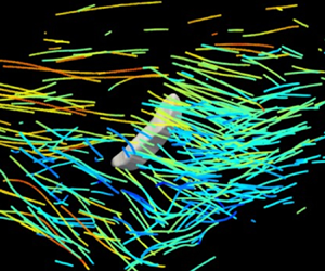
Figure 4(a) shows an example of a bubble experiencing strong turbulent strains, illustrated by many tracer tracks that are colour-coded with their instantaneous velocity magnitude. Although the flow field is complicated and contains dynamics over multiple scales, the estimated  $\tilde {S}_{ij}$ coarse-grained at the bubble scale is sketched in figure 4(c). For this case,
 $\hat {\boldsymbol {e}}_3$ clearly aligns with the bubble semi-minor axis
 $\hat {\boldsymbol {r}}_3$, whereas
 $\hat {\boldsymbol {e}}_1$ aligns with the bubble semi-major axis
 $\hat {\boldsymbol {r}}_1$. This result is consistent with our expectations, but it is important to collect statistics concerning such relative orientation to ensure that this example is not an isolated case.
Reconstructed 3-D shape of deforming bubbles with surrounding tracer trajectories (the instantaneous velocity magnitude  $u$ of each particle is indicated by the colour), including (a) a case that is primarily deformed by turbulent strain and (b) another case that is primarily deformed by the slip velocity. (c,d) Schematics of the coarse-grained flow field around these two bubbles.

Another driving mechanism for bubble deformation is the slip velocity  $\boldsymbol {u}_{slip} = \boldsymbol {u}_{\boldsymbol {b}} - \boldsymbol {u}_{\boldsymbol {f}}$ between the two phases. Bubbles subjected to
 $\boldsymbol {u}_{slip}$ will experience a motion-induced pressure gradient and thus deform, which can be measured by another Weber number:
 $We_{slip}=\rho u_{slip}^2 D/\sigma$.
 $We_{slip}$ can be defined either using the total slip velocity or one of its three components, i.e.
 $We_{slip,x}$,
 $We_{slip,y}$ and
 $We_{slip,z}$. The slip velocity could arise due to multiple effects: (i) the buoyancy effect is the strongest for bubbles rising in an otherwise quiescent medium, in which the bubble deformation is primarily driven by the slip velocity along the vertical direction; (ii) the added mass force, which is important for bubbles travelling in turbulence with large carrier-phase acceleration; (iii) the finite size effect could also lead to a large slip velocity between the two phases (Bellani & Variano Reference Bellani and Variano2012; Cisse, Homann & Bec Reference Cisse, Homann and Bec2013). Figure 4(b) shows an example of a bubble subjected to a strong slip velocity along the horizontal direction. After coarse-graining the flow field, figure 4(d) illustrates the mean flow around the bubble, which is primarily along the horizontal direction. At the same time, the bubble slides along the cyan arrow. As a result, the slip velocity points in a direction indicated by the red arrow, which aligns excellently with the direction of the semi-minor axis
 $\hat {\boldsymbol {r}}_3$ of the reconstructed bubble geometry.
3. Results and discussion
3.1. Alignment and orientation of deforming bubbles
Figure 5 shows the p.d.f. of the cosine of the angle ( $W$) between two unit vectors. If two unit vectors are randomly oriented, the p.d.f. should be close to a uniform distribution (
 ${p}(W)=1$ for all
 $W$, where
 $p(\dotsb )$ represents the probability). A peak at
 $W=1$ in the p.d.f. would suggest a preferential alignment between the two vectors, whereas a peak near
 $W=0$ would imply that the two vectors are perpendicular to each other. Figure 5(a) shows the orientation of the slip velocity
 $\hat {\boldsymbol {u}}_{slip}$ with respect to
 $\hat {\boldsymbol {r}}_1$ and
 $\hat {\boldsymbol {r}}_3$. There is a clear preferential alignment between
 $\hat {\boldsymbol {u}}_{slip}$ and
 $\hat {\boldsymbol {r}}_3$, which suggests that the pressure gradient induced by the bubble's relative motion compresses the bubble along this direction.
Probability density function of the cosine of the angle between bubble axes with (a) the slip velocity and (b) the turbulent strain rate.

In addition to compression, bubbles must extend in other directions to conserve volume. However,  $\hat {\boldsymbol {r}}_1$ is not forced to be orthogonal to
 $\hat {\boldsymbol {r}}_3$ during the 3-D reconstruction to allow the capture of any non-affine deformation. Thus, the preference of
 $\hat {\boldsymbol {r}}_1$ being perpendicular to
 $\hat {\boldsymbol {u}}_{slip}$ is not as strong as that of
 $\hat {\boldsymbol {r}}_3$ being aligned with
 $\hat {\boldsymbol {u}}_{slip}$. Such a difference also suggests that the orientation of a deformable bubble is primarily determined by the slip velocity compressing the bubble.
The contribution from the surrounding turbulent strain rate to the orientation of the bubbles is also shown in figure 5(b).  $\hat {\boldsymbol {r}}_1$ and
 $\hat {\boldsymbol {r}}_3$ clearly preferentially align with
 $\hat {\boldsymbol {e}}_1$ and
 $\hat {\boldsymbol {e}}_3$, respectively. The alignment between
 $\hat {\boldsymbol {r}}_3$ and
 $\hat {\boldsymbol {e}}_3$ is slightly stronger, suggesting a more important role played by the flow compression. The small difference implies that, although the bubble deformation is driven by flow compression, bubbles must be stretched along other directions with the least resistance; this happens to be
 $\hat {\boldsymbol {r}}_1$ if only the strain rate tensor is considered.
The preferential alignment between bubble axes with the eigenvectors of the strain rate tensor is significantly weaker compared to that with the slip velocity, despite the similarity of their respective Weber numbers (Masuk et al. Reference Masuk, Salibindla and Ni2021). A reason for this is that the slip velocity is associated with large-scale flow motions, which can be sustained longer compared with the strain rate. Therefore, the bubble orientation may be more dominated by the slip velocity. In addition, the slip velocity and turbulent strain rate do not always work collaboratively. Figure 5(a) shows the p.d.f. of the relative orientation between  $\hat {\boldsymbol {e}}_3$ and
 $\hat {\boldsymbol {u}}_{slip}$, which seems to be a nearly random distribution and may slightly prefer a perpendicular orientation. This suggests that these two mechanisms are not correlated and may even occasionally compete with each other, and therefore a preferential alignment with the slip velocity may lead to a weaker alignment with turbulent strain rate and vice versa.
If the bubble shape can be assumed as a triaxial ellipsoid without any non-affine deformation, it can be captured as a symmetric, positive definite, second-rank tensor  $\boldsymbol {P}$. The phenomenological equation to describe the time evolution of
 $\boldsymbol {P}$ was provided by Maffettone & Minale (Reference Maffettone and Minale1998):
 \begin{equation} \frac{\textrm{d}\boldsymbol{P}}{\textrm{d}t}-(\boldsymbol{\varOmega}\boldsymbol{\cdot}\boldsymbol{P}-\boldsymbol{P}\boldsymbol{\cdot} \boldsymbol{\varOmega})={-}\,\frac{f_1}{\tau}\left(\boldsymbol{P}-g(\boldsymbol{P})\boldsymbol{I}\right)+\,f_2( \boldsymbol{S}\boldsymbol{\cdot}\boldsymbol{P}+\boldsymbol{P}\boldsymbol{\cdot}\boldsymbol{S}), \end{equation}
where  $\boldsymbol {S}$ and
 $\boldsymbol {\varOmega }$ represent the symmetric and anti-symmetric parts of the velocity gradient tensor;
 $\tau =\mu D/2\sigma$ is the interfacial relaxation timescale;
 $\mu$ and
 $\sigma$ are the dynamic viscosity and the surface tension of water, respectively; and
 $\boldsymbol {I}$ is the second-rank unit tensor. The equation has two main contributions, deformation and restoration (the first term on the right-hand side), where
 $f_1$ and
 $f_2$ are two coefficients associated with the viscosity ratio, and
 $g(\boldsymbol {P})$ is introduced to preserve the bubble volume.
Strictly speaking, equation (3.1) should not be applied to finite-sized bubbles since the model assumes a linear flow around the bubble, which should be limited solely to bubbles with size  $D\ll \eta$. Moreover, this equation does not consider the slip velocity or the buoyancy effect owing to a significant density mismatch between the two phases. Nevertheless, when ignoring this mismatch and replacing
 $\boldsymbol {S}$ and
 $\boldsymbol {\varOmega }$ with their coarse-grained counterparts, this equation can estimate the alignment between a deforming neutrally buoyant droplet and its surrounding coarse-grained strain rate.
If the restoring term led by the surface tension is ignored for further simplification, the equation restores to the deformation equation of a material element (Girimaji & Pope Reference Girimaji and Pope1990),  $\textrm {d}\boldsymbol {F}/\textrm {d}t=\boldsymbol {A}\boldsymbol {\cdot }\boldsymbol {F}$, where
 $\boldsymbol {F}$ is the deformation tensor and can be converted to a left
 $\boldsymbol {C}^{(L)}$ or right
 $\boldsymbol {C}^{(R)}$ Cauchy–Green strain tensor using
 $\boldsymbol {C}^{(L)}=\boldsymbol {F}\boldsymbol {\cdot }\boldsymbol {F}^{T}$ and
 $\boldsymbol {C}^{(R)}=\boldsymbol {F}^{T}\boldsymbol {\cdot }\boldsymbol {F}$. One can prove that
 $\boldsymbol {C}^{(L)}\equiv \boldsymbol {P}$, which suggests that a bubble without surface tension will be deformed by turbulence similarly to the deformation process of a material element, whose three semi-major axes can be determined based on the eigenvectors of
 $\boldsymbol {C}^{(L)}$. The deformation equation can be integrated to obtain
 $\boldsymbol {C}^{(L)}$ as reported in Ni et al. (Reference Ni, Kramel, Ouellette and Voth2015), using the simulation results by Benzi et al. (Reference Benzi, Biferale, Calzavarini, Lohse and Toschi2009). Although the eigenvalues of
 $\boldsymbol {C}^{(L)}$ grow exponentially as the integration time increases, the eigenvectors of
 $\boldsymbol {C}^{(L)}$,
 $\hat {\boldsymbol {e}}_{Li}$ vary by only a little and they can be used to represent the directions of neutrally buoyant droplets with zero surface tension.
Figure 6 shows the relative orientation between the semi-major axis of the deformed material element  $\hat {\boldsymbol {e}}_{L1}$ with three eigenvectors,
 $\hat {\boldsymbol {e}}_i$, of the strain rate tensor as well as with the vorticity vector
 $\hat {\boldsymbol {\omega }}$. It has been discussed before by Ni et al. (Reference Ni, Kramel, Ouellette and Voth2015), that the strongest alignment is observed between the semi-major axis of the material element and the vorticity vector because vorticity is amplified by the vortex stretching process. As a vortex is stretched by the Lagrangian stretching
 $\boldsymbol {C}^{(L)}$, it ends up aligning with
 $\hat {\boldsymbol {e}}_{L1}$.
Probability density function of the cosine of the angle between the semi-major axis of material elements  $\hat {\boldsymbol {e}}_{L1}$ and both vorticity
 $\hat {\boldsymbol {\omega }}$ and eigenvectors of the strain-rate tensor,
 $\hat {\boldsymbol {e}}_i$.

When comparing figures 5 and 6, the semi-major axis of a material element,  $\hat {\boldsymbol {e}}_{L1}$, shows strong alignment with
 $\hat {\boldsymbol {e}}_2$ and
 $\hat {\boldsymbol {\omega }}$, whereas the semi-major axis
 $\hat {\boldsymbol {r}}_1$ of finite-sized bubbles does not appear to have strong preferential orientation. This finding is qualitatively consistent with the work conducted by Biferale et al. (Reference Biferale, Meneveau and Verzicco2014), who showed that, for a small capillary number, the alignment between the semi-major axis of the neutrally buoyant droplets with
 $\hat {\boldsymbol {\omega }}$ is relatively weak; in addition, as the capillary number increases, the alignment becomes stronger. This observation suggests that, despite the differences in Reynolds number and sizes, our results for the orientational dynamics of finite-sized bubbles share similarities with the sub-Kolmogorov-scale neutrally buoyant droplets at a small capillary number.
Nevertheless, the alignment of finite-sized bubbles with the coarse-grained strain rate is much weaker than that for sub-Kolmogorov-scale droplets, which is mainly caused by: (i) the competing effect from the slip velocity and (ii) the non-affine deformation allowed by our shape reconstruction method, meaning that the semi-major and semi-minor axes of the bubbles are not necessarily orthogonal, which would weaken the alignment with the eigenvectors of the coarse-grained turbulent strain rate.
3.2. Breakup
The previous section discussed statistics concerning the alignment between the semi-major and semi-minor axes of deforming bubbles and the slip velocity and velocity gradients. To collect sufficient statistics, bubbles with different aspect ratios and sizes were compiled together. This data can help us to answer whether the alignment depends on how strongly the bubble is deformed and whether the roles played by different mechanisms change when bubbles experience strong deformation. In this section, we will examine bubbles with strong deformation and that are close to the breakup moments, to unveil key mechanisms behind bubble breakup in turbulence.
The slip velocity and turbulent strain rate can be tracked along each bubble trajectory. For all our experiments, 190 datasets were collected, from which a total of 480 329 bubbles were reconstructed and tracked over time. The majority did not break during the time spent in the view volume, and only 195 breakup events were identified and reconstructed. Details concerning the reconstruction of the breakup events can be found in Masuk et al. (Reference Masuk, Salibindla and Ni2019a) and Qi, Masuk & Ni (Reference Qi, Masuk and Ni2020).
For all these breakup events, time traces of  $We_{slip,x}$ and
 $We_{vg}$ before breakups are compiled to calculate the time evolution of the Weber numbers. Figure 7 shows the p.d.f.s of
 $We_{slip,x}$ and
 $We_{vg}$ at different times before breakup. The closest and the farthest times tracked before the breakup were approximately
 $0.5\tau _{\eta }$ and
 $20\tau _{\eta }$, respectively. We also plot the p.d.f.s of
 $We_{slip,x}$ and
 $We_{vg}$ for all bubbles, including both weak and strong deformation cases, in figure 7(a,b) as black solid circles. They show that the Weber numbers for bubbles about to break are systematically larger than those for non-breaking bubbles with a similar size. In addition,
 $We_{slip,x}$ continues to grow from
 $20 \tau _\eta$ to
 $5 \tau _\eta$; however, from
 $2\tau _\eta$ to the moment of breakup, the distribution leaps far rightward to a larger
 $We_{slip,x}$. This indicates that the bubble breakup is associated with a timescale that is within
 ${\sim }2\tau _\eta$, over which the slip velocity experiences dramatic changes. The same calculation was performed for
 $We_{vg}$; unlike the case for
 $We_{slip,x}$, however, the distribution of
 $We_{vg}$ does not seem to experience a systematical shift over time. Nevertheless, the left tail for small
 $We_{vg}$ seems to shift rightward as bubbles approach breakup, which indicates that the number of events with small velocity gradients declines near breakup. In contrast to the time evolution of
 $We_{slip,x}$ and
 $We_{vg}$ for breaking bubbles only, the distribution of these two Weber numbers (shown as black solid symbols in figure 7a,b) for all bubbles are quite close to each other and both peak at around
 $We\approx 1$.
Probability density function of (a) the slip-velocity-based Weber number and (b) the strain-rate-based Weber number, for mild deformation case (black solid symbols) as well as different times ( $\tau _0$) before breakup.

In addition to the Weber numbers, figure 8 shows the alignment of the slip velocity with the semi-major axis of the bubble for (i) all bubbles, (ii) the breaking bubbles ( $5 \tau _{\eta }$ prior to the breakup) and (iii) the breaking bubbles (
 $20 \tau _{\eta }$ prior to the breakup). The results suggest a consistent trend of the bubble semi-major axis flipping from a perpendicular to a parallel orientation relative to the slip velocity direction, which seems to contradict the discussion in § 3.1 that slip velocity should flatten rather than elongate the bubble along its direction.
Probability density function of the cosine of the angle between the bubble semi-major axis  $\hat {\boldsymbol {r}}_1$ and the slip velocity
 $\hat {\boldsymbol {u}}_{slip}$ for mild deformation and two different time (
 $\tau _0$) before breakup.

This surprising behaviour will be explained later after discussing the relative orientation of the bubble semi-major axis with the eigenvectors of the strain rate tensor. Figure 9(a) shows the distribution of the alignment of the bubble semi-major axis with  $\hat {\boldsymbol {e}}_3$ similar to figure 5(b). Here, the distribution is shown as a function of the time before the breakup event. As we discussed in § 3.1, the bubble semi-major axis prefers a slightly perpendicular orientation with
 $\hat {\boldsymbol {e}}_3$. Unlike with slip velocity, this preference becomes even stronger as bubbles approach breakup over time, which is clear from figure 9(a).
Probability density function of the cosine of the angle between the bubble semi-major axis  $\hat {\boldsymbol {r}}_1$ and the smallest eigenvector of the strain-rate tensor
 $\hat {\boldsymbol {e}}_3$ for (a) different times (
 $\tau _0$) before breakup and (b) all strongly deformed (aspect ratio
 $\alpha >2.5$) cases.

Although the distribution of  $We_{vg}$ measuring the magnitude of the driving force changes by little over time (figure 7), the strain rate seems to more effectively compress the bubble as
 $\hat {\boldsymbol {e}}_3$ becomes more perpendicular to
 $\hat {r}_1$ and better aligns with
 $\hat {r}_3$ over time; however, the p.d.f.s of the relative orientation are noisy due to the limited number of breakup events. To verify this observed trend, figure 9(b) shows the p.d.f. for the same relative orientation but only for cases when bubbles experienced significant deformation (
 $\alpha >2.5$) but did not break, and the results show a similar trend to what has been observed for breaking bubbles close to the breakup moment. This supports the conjecture that the flow compression around bubbles does not become larger, but becomes more effective as it better aligns with bubbles as they approach breakup or strong deformation.
Based on the observation of the relative orientation between  $\hat {\boldsymbol {r}}_1$ and the slip velocity (
 $\hat {\boldsymbol {u}}_{slip}$) or between
 $\hat {\boldsymbol {r}}_1$ and the strain rate (
 $\hat {\boldsymbol {e}}_3$), before bubbles break, the slip velocity becomes stronger in magnitude, and the velocity gradient aligns better with bubbles and consequently breaks the bubble more effectively. Each mechanism seems to adjust in a different manner to aid breakup. The surprising nearly
 $90^{\circ }$ rotation of the relative orientation between the slip velocity and
 $\hat {\boldsymbol {r}}_1$ is caused by the fact that the slip velocity contains contributions from both bubbles and their surrounding flows. When the bubble deformation is weak, the slip velocity serves as the driving mechanism for bubble deformation. As bubbles approach breakup and deform significantly, their velocity increases and overtakes the direction of the slip velocity. Because the bubble velocity during strong deformation aligns with
 $\hat {\boldsymbol {r}}_1$, the slip velocity becomes aligned with the semi-major axis. In other words, the slip velocity transitions from the driving mechanism to the driven result owing to the contributions from both phases.
The measured orientational dynamics during deformation and breakup paints a different physical picture compared with the popular bubble-eddy collision model, which is used extensively in the population balance equation to calculate the bubble breakup probability (Luo & Svendsen Reference Luo and Svendsen1996; Lehr, Millies & Mewes Reference Lehr, Millies and Mewes2002; Wang, Wang & Jin Reference Wang, Wang and Jin2003; Liao & Lucas Reference Liao and Lucas2009). This model assumes that bubble breakup is driven by the collision with turbulent eddies of size equal to or smaller than the bubble size, and it has to assume a breakup criteria based on the difference or ratio between the eddy kinetic energy and the surface energy, which is similar to the critical Weber number criteria. In the bubble-eddy collision model, the contribution of the slip velocity was not considered, although it represents an important deformation mechanism for finite-sized bubbles, as shown in our work. The bubble-eddy collision model also implies that the Weber number should increase when the bubble encounters a strong eddy; however, we observed no change in the distribution of the Weber number based on the strain rate as bubbles approach breakup. Instead, the bubble orientation shows better alignment with the local strain rate to facilitate bubble breakup. Furthermore, although the slip velocity plays a more dominant role in determining the orientation of weakly deformed bubbles, the strain rate tensor seems to be more important for breaking bubbles. It remains unclear why these two mechanisms switch their roles between deformation and breakup, and thus requires further investigation to appropriately capture it in models.
4. Conclusion
This paper describes an experimental study of the orientational dynamics of deformed finite-sized bubbles in homogeneous and isotropic turbulence with a large energy dissipation rate. Both the bubble geometry and many surrounding tracer particles have been simultaneously reconstructed and tracked in three dimensions. From this unique data set, the relative orientation between bubbles and two driving mechanisms, i.e. slip velocity and the strain rate, can be extracted.
For mild deformation, the strongest alignment is observed between the bubble semi-minor axis and slip velocity, which suggests that bubbles are predominately compressed by the slip velocity. In addition, the bubble semi-major and semi-minor axes are aligned with the strongest stretching and compression directions of the strain rate tensor coarse-grained at the bubble size, respectively. Compared to the relative orientation of the bubbles with the slip velocity, their alignment with the strain rate tensor is weaker and could be affected by the competition between deformation driven by the strain rate and deformation driven by the slip velocity.
The orientational dynamics of deformable bubbles are also compared to that of neutrally buoyant sub-Kolmogorov-scale material elements with no surface tension or slip velocity. Their orientations show strong alignment with the vorticity vector and the intermediate eigenvector of the turbulent strain rate. But such an alignment is absent for finite-sized bubbles in our experiments. This observed difference qualitatively agrees with a previous simulation on sub-Kolmogorov-scale droplets with different capillary numbers, indicating that the restoring force from the surface tension could strongly affect the bubble orientation.
Finally, the orientational dynamics of strongly deformed bubbles is studied, particularly for events near breakup. As bubbles approach breakup, the preference for a perpendicular orientation between  $\hat {\boldsymbol {e}}_3$ and
 $\hat {\boldsymbol {r}}_1$ grows, which leads to a more effective strain-induced deformation. The alignment between
 $\hat {\boldsymbol {u}}_{slip}$ and the bubble semi-major axis (
 $\hat {\boldsymbol {r}}_1$) transitions from perpendicular to aligned. This transition was explained by the slip velocity switching from a driving mechanism to the driven result as the strong deformation begins to affect the bubble translational velocity.
Funding
We acknowledge the financial support from the National Science Foundation under the award numbers 1854475 and CAREER-1905103.
Declaration of interests
The authors report no conflict of interest.