
1. Introduction
Time-periodic fluid flows are ubiquitous by nature, examples are the pulsatile flow of blood, rotating flows in turbomachines and engines, and vortex shedding in the wake of bluff bodies. Controlling fluid flows (Bewley Reference Bewley2001; Kim & Bewley Reference Kim and Bewley2007; Brunton & Noack Reference Brunton and Noack2015), and periodic vortex shedding specifically (Colonius & Williams Reference Colonius and Williams2011), has remained a significant engineering challenge, with potential impact for industry and technology. Despite the challenges of flow control, researchers have long been inspired and encouraged by the exceptional performance of biological flyers and swimmers that take advantage of unsteady aerodynamics through flapping in order to effect phenomenal manoeuvrability in a range of flow conditions (Dickinson, Lehmann & Sane Reference Dickinson, Lehmann and Sane1999; Shyy et al. Reference Shyy, Lian, Tang, Viieru and Liu2008; Ramananarivo, Godoy-Diana & Thiria Reference Ramananarivo, Godoy-Diana and Thiria2011; Wu Reference Wu2011). To achieve such performance, even in high-amplitude gusting conditions, the animal must sense the flow and adjust its wings or fins in real time (Shyy et al. Reference Shyy, Kang, Chirarattananon, Ravi and Liu2016). For instance, Dickinson et al. (Reference Dickinson, Lehmann and Sane1999) suggested that regulating the phase of wing rotation effectively controls the aerodynamic forces during manoeuvres. The wing motion is, in turn, regulated by modifying the activation phase of the associated muscles (Dickinson et al. Reference Dickinson, Farley, Full, Koehl, Kram and Lehman2000), which involves precise timing modulation (Sponberg & Daniel Reference Sponberg and Daniel2012). Inspired by these natural systems, there are ongoing efforts to develop simple yet robust control laws for engineering time-periodic flows, albeit with less emphasis on precise timing modulation.
Established controllers for unsteady fluid flows typically rely on steady or quasi-steady assumptions and implementation within predefined ranges of uncertainty and perturbations. Moreover, linearising the flow about a steady base state is often inadequate to control large-amplitude flow unsteadiness owing to the challenges of high-dimensionality, strong nonlinearity and time delays (Bewley Reference Bewley2001; Brunton & Noack Reference Brunton and Noack2015; Brunton, Noack & Koumoutsakos Reference Brunton, Noack and Koumoutsakos2020). One of the main approaches for analysing perturbation dynamics about time-varying periodic base states is Floquet analysis (Herbert, Bertolotti & Santos Reference Herbert, Bertolotti and Santos1987; Barkley & Henderson Reference Barkley and Henderson1996). Here, the flow is linearised about the periodic base state and the amplification of perturbations about this state is determined by the magnitude of the Floquet exponents. In the work by Giannetti, Camarri & Citro (Reference Giannetti, Camarri and Citro2019), a combination of Floquet analysis and adjoint-based sensitivity analysis was used to identify effective regions for flow control. Phase-amplitude reduction provides a complementary approach to Floquet analysis, enabling a reduced-order description of the phase and amplitude sensitivity of perturbations about limit-cycle oscillations (Nakao Reference Nakao2016; Wilson & Moehlis Reference Wilson and Moehlis2016). In fact, phase and amplitude reduction yield the left Floquet eigenvectors associated with the zero and higher Floquet exponents, respectively, (Kuramoto & Nakao Reference Kuramoto and Nakao2019; Takata, Kato & Nakao Reference Takata, Kato and Nakao2021) and are eigenfunctions of the infinite-dimensional Koopman operator (Mezić Reference Mezić2005; Mauroy, Mezić & Moehlis Reference Mauroy, Mezić and Moehlis2013). As we restrict our attention to timing modulation of periodic fluid flows in this work, we only perform phase reduction. Although phase reduction is well established in the study of limit-cycle oscillators in neuroscience (Malkin Reference Malkin1949; Kuramoto Reference Kuramoto1984; Winfree Reference Winfree2001), its use for fluid flows has only recently gained traction. Phase-reduction analysis collapses the high-dimensional dynamics to that of a single scalar phase variable. The collective phase description of oscillatory convection was first introduced in the works of Kawamura & Nakao (Reference Kawamura and Nakao2013, Reference Kawamura and Nakao2015). More recently, Taira & Nakao (Reference Taira and Nakao2018) used a phase-reduction approach to analyse synchronisation of perturbation dynamics about time-varying base states for unsteady wake flows. Using this approach, the conditions for synchronisation (lock-on) to external excitation were determined (Munday & Taira Reference Munday and Taira2013). Moreover, phase-based characterisation of the global flow field around a bluff body (Khodkar & Taira Reference Khodkar and Taira2020) and sensitivity of phase dynamics to body motion (Khodkar, Klamo & Taira Reference Khodkar, Klamo and Taira2021) have been studied. Such a phase-reduced representation of the flow physics forms the basis of the analysis in this work. In using the lock-on conditions, simple controllers can be designed such that the phase of the oscillations can be altered asymptotically. However, in this work, we aim to deduce the optimal external excitation over a time scale commensurate with variations in the base state of the flow. The present work shares similarities with the seminal work of Pastoor et al. (Reference Pastoor, Henning, Noack, King and Tadmor2008) where they designed a phase controller for turbulent flow around a D-shaped body. Here, the mechanism of phase control explicitly synchronises the upper and lower shear-layer development. By delaying the formation of vortex shedding at low control amplitudes, this phase control is able to achieve considerable drag reduction. However, the control requires substantial effort in designing a nonlinear reduced-order vortex model for tracking and predicting the dependence of the vortex shedding phase on control inputs. Here, we describe these dependencies of vortex shedding phase on control inputs through a simple sensor-based phase-reduction framework.
The objective of the present work is to perform rapid control of unsteady periodic flows. To this end, we develop a phase-response model that precisely characterises the transient responses and subsequently alters the transient flow characteristics in a time scale commensurate with the base-flow oscillation. Furthermore, we only track the phase variations in the aerodynamic forces in bluff-body wake flows, and not the entire flow field, to develop the phase-response model; we assume that the aerodynamic forces are obtained through sensor measurements. Such an observable phase-reduction strategy greatly simplifies and improves the feasibility of the present approach for use in an experimental setting. We then leverage recent developments in variational methods that determine the optimal control inputs altering the transient behaviour of spiking neurons (Moehlis, Shea-Brown & Rabitz Reference Moehlis, Shea-Brown and Rabitz2006; Monga et al. Reference Monga, Wilson, Matchen and Moehlis2019), extending the method to enable transient flow control. An alternative closed-loop model predictive control strategy for transient phase control is also proposed for comparison with the variational method. Altering the phase of the vortex shedding also affects the transient amplitude of the unsteady aerodynamic forces. This change in amplitude, although an indirect effect of phase alteration, is a welcome consequence of the control strategy. The present approach is demonstrated on relevant examples, including the Stuart–Landau (SL) oscillator model, and laminar flows past a cylinder and over an airfoil. In each example, we demonstrate the strength of the proposed approach, as well as the ability to incorporate physically realistic measurements and actuation strategies. Based on the phase-reduction analysis, we introduce two control optimisation strategies, based on the Euler–Lagrange equations and model predictive control. This formulation enables the real-time control of the phase of vortex shedding, including prescribing the desired time of vortex pinch-off. The ability to modify the phase dynamics of time-varying vortical flows accelerates or decelerates the associated vortex shedding process, which in turn affects the unsteady aerodynamic forces.
2. Formulation
Our main goal is to characterise and control the phase dynamics of oscillatory dynamical systems of the form
 \begin{equation} \dot{\boldsymbol{q}} = \boldsymbol{N}(\boldsymbol{q}) + \boldsymbol{f}, \end{equation}
where  $\boldsymbol {q}$ is the state variable and
 $\boldsymbol {f}$ is the external forcing or control input. The evolution of the fluid flows in this paper are governed by the non-dimensional, incompressible, Navier–Stokes equation with forcing
 \begin{equation} \underbrace{\frac{\partial \boldsymbol{q}}{\partial t}}_{\dot{\boldsymbol{q}}} = \underbrace{-(\boldsymbol{q} \boldsymbol{\cdot} \boldsymbol{\nabla}) \boldsymbol{q} - \boldsymbol{\nabla} p + \frac{1}{Re} \nabla^2 \boldsymbol{q}}_{\boldsymbol{N(\boldsymbol{q})}} + \boldsymbol{f},\quad \boldsymbol{\nabla} \boldsymbol{\cdot} \boldsymbol{q} = \boldsymbol{0}, \end{equation}
where  $\boldsymbol {q} = \boldsymbol {q}(\boldsymbol {x},t)$ is the velocity vector field,
 $p$ is the scalar pressure field and
 $\boldsymbol {f} = \boldsymbol {f}(\boldsymbol {x},t)$ is the external perturbation/forcing (actuation) defined over a spatial coordinate
 $\boldsymbol {x}$ and time
 $t$. Here,
 $Re$ is the Reynolds number. A large class of unsteady fluid flows have a time-periodic solution
 $\boldsymbol {q}_0$ (i.e. a limit-cycle) satisfying
 \begin{equation} \dot{\boldsymbol{q}}_0 = \boldsymbol{N}(\boldsymbol{q}_0),\quad \boldsymbol{q}_0(\boldsymbol{x},t) = \boldsymbol{q}_0(\boldsymbol{x},t+T), \end{equation}
where  $T$ is the fundamental time period of the flow
 $\boldsymbol {q}_0$. The corresponding natural frequency of oscillation is
 $\omega _n = 2{\rm \pi} /T$. We focus on such time-periodic flows in this work. Our work is inspired by two threads of prior work to determine the energy-optimal phase-control input
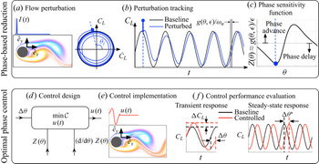
 $\boldsymbol {f}(\boldsymbol {x},t)$: phase-reduction analysis for fluid flows (Taira & Nakao Reference Taira and Nakao2018) and energy-optimal phase control for neuronal systems (Moehlis et al. Reference Moehlis, Shea-Brown and Rabitz2006). Combining these approaches results in a strategy for energy-optimal phase control of time-periodic fluid flows, summarised in figure 1.
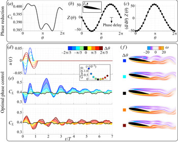
Overview of phase-reduction analysis: (a) introduction of impulse flow perturbation, (b) baseline and perturbed lift coefficient trajectories (left, phase portrait of oscillations in  $\dot {C}_L\text {-}C_L$ plane; right, time history) and (c) phase-sensitivity function
 $\boldsymbol {Z}(\theta )$. Overview of energy-optimal phase control: (d) design of optimal control input
 $u(t)$ for desired phase shift
 $\Delta \theta$ and (e) controlled flow with the forcing
 $\boldsymbol {f}(t)$; (f) transient and steady-state response of lift coefficient on application of control.

The overall procedure is carried out in two stages, as follows.
(i) Phase-reduction analysis: following the work of Nakao (Reference Nakao2016) and Taira & Nakao (Reference Taira and Nakao2018), phase-reduction analysis is used to describe the the phase behaviour of periodic wake flows. Introducing perturbations to the flow at various phases of oscillation, the phase sensitivity of the perturbations are tracked compared to the baseline oscillation, and a phase-based reduced-order model is constructed. This model describes the phase dynamics of perturbations about the time-periodic base state. This modelling procedure is explained in more detail in § 2.1.
(ii) Optimal phase control: in this stage, we extend the optimal control strategy developed by Moehlis et al. (Reference Moehlis, Shea-Brown and Rabitz2006) to time-periodic fluid flows. We alter the phase dynamics of fluid flows on a time scale that is commensurate with the fundamental time period
 $T$ of the bluff-body flow. The open-loop control input is determined for desired phase alteration using the phase-reduced model and the Euler–Lagrange equations. These control inputs are added to the flow, and the transient and steady-state control response, along with the associated flow physics, are examined. This optimal phase-control procedure is described in detail in § 2.3.

Specific aims of the present work are to: (i) achieve a transient phase shift by a desired amount within the fundamental time period of base flow oscillation, (ii) explore the indirect change in the aerodynamic coefficients in the immediate transient after application of control for various phase alterations, and (iii) investigate the implications of phase control on the vortex formation and shedding process.
2.1. Phase-reduction analysis
The phase dynamics of the time-periodic solution  $\boldsymbol {q}_0$ of the unforced system, with frequency
 $\omega _n$, is given by
 \begin{equation} \dot{\theta}(t) = \omega_n,\quad \theta \in [-{\rm \pi},{\rm \pi}], \end{equation}
where  $\theta$ is the phase of the limit-cycle oscillation. Solutions
 $\boldsymbol {q}$ at each spatial coordinate
 $\boldsymbol {x}$ on the limit cycle will have the frequency
 $\omega _n$, although they will have different phases. We define this by the scalar phase function
 $\varTheta (\boldsymbol {q})$. Furthermore,
 $\varTheta (\boldsymbol {q})$ extends
 $\theta$ in the neighbourhood of the limit cycle
 $\boldsymbol {q}_0$ and provides the phase for
 $\boldsymbol {q}$ in general. Combining with (2.4), the time derivative of the scalar phase function is given by
 \begin{equation} \dot{\theta}(t) = \dot{\varTheta}(\boldsymbol{q}) = \boldsymbol{\nabla}_{\boldsymbol{q}} \varTheta(\boldsymbol{q})|_{\boldsymbol{q}_0} \boldsymbol{\cdot} \dot{\boldsymbol{q}} = \boldsymbol{\nabla}_{\boldsymbol{q}} \varTheta(\boldsymbol{q})|_{\boldsymbol{q}_0} \boldsymbol{\cdot} \boldsymbol{N}(\boldsymbol{q}) = \omega_n. \end{equation}
Here, the time derivative of the scalar phase function is expanded using the chain rule with the derivative with respect to  $\boldsymbol {q}$ evaluated at time-periodic solution
 $\boldsymbol {q}_0$.
To deduce the phase reduction of the perturbed/forced system given by (2.5), we introduce small perturbations to the flow at characteristic phases  $\theta$ such that
 $\boldsymbol {f}(\boldsymbol {x},t) = I(t)\boldsymbol {h}(\boldsymbol {x}) = \epsilon \delta (t-t_0)\boldsymbol {h}(\boldsymbol {x})$, where
 $\epsilon \ll 1$,
 $\boldsymbol {h}(\boldsymbol {x})$ is a spatial forcing profile with
 $\|\boldsymbol {h}\|=1$ and
 $\delta$ is a unit-area delta function. The delta function is centred at time
 $t_0\in [0,T]$ corresponding to characteristic phases
 $\theta$ at which perturbations are introduced. Considering only the first-order effects of the introduced perturbation near the time-periodic solution, we obtain
 \begin{equation} \dot{\varTheta}(\boldsymbol{q}) = \boldsymbol{\nabla}_{\boldsymbol{q}} \varTheta(\boldsymbol{q})|_{\boldsymbol{q}_0} \boldsymbol{\cdot} (\boldsymbol{N}(\boldsymbol{q}) + \boldsymbol{f}) = \omega_n + \epsilon \delta(t-t_0) \boldsymbol{\nabla}_{\boldsymbol{q}} \varTheta(\boldsymbol{q})|_{\boldsymbol{q}_0} \boldsymbol{\cdot} \boldsymbol{h}, \end{equation}
where the term  $\boldsymbol {\zeta }(\theta ) = \boldsymbol {\nabla }_{\boldsymbol {q}} \varTheta (\boldsymbol {q})|_{\boldsymbol {q}_0}$ is called as the phase-sensitivity function. The level sets of the phase function
 $\varTheta (\boldsymbol {q})$ constitute the phase-reduced coordinates, which are directly perpendicular to the phase-sensitivity function
 $\boldsymbol {\zeta }(\theta )$ (Guckenheimer Reference Guckenheimer1975). Thus, the phase dynamics can be linearly approximated through the phase-reduced model
 \begin{equation} \dot{\theta}(t) = \omega_n + \boldsymbol{\zeta}(\theta) \boldsymbol{\cdot} \boldsymbol{f} = \omega_n + \epsilon \delta(t-t_0)\boldsymbol{\zeta}(\theta) \boldsymbol{\cdot} \boldsymbol{h}(\boldsymbol{x}),\quad \theta \in [-{\rm \pi},{\rm \pi}], \end{equation}
where  $\theta$ is the phase of the limit-cycle oscillation. Next, we describe our system identification approach to determine the phase-sensitivity function.
2.2. Sensor-based phase-sensitivity function
To evaluate  $\boldsymbol {\zeta }(\theta )$, given an actuation strategy with spatial profile
 $\boldsymbol {h}(\boldsymbol {x})$, small impulsive perturbations are introduced to the flow of the form,
 \begin{equation} I(t) = \epsilon\delta(t-t_0) = \frac{\epsilon}{\sqrt{2{\rm \pi}}\sigma} \exp{\left[-\frac{1}{2}\left(\frac{t-t_0}{\sigma}\right)^2\right]}, \end{equation}
where  $t_0$ corresponds to the time at a particular phase of the flow
 $\theta (t_0)$ when the impulse is introduced. For all cases considered in this work,
 $\sigma = 10\Delta t$, where
 $\Delta t$ is the numerical time step. The spatial profile
 $\boldsymbol {h}(\boldsymbol {x})$ depends on the type of actuation considered.
To compute the phase-sensitivity function  $\boldsymbol {\zeta }(\theta )$, one approach is to solve an associated adjoint problem to (2.6) with Malkin's normalisation condition (Brown, Moehlis & Holmes Reference Brown, Moehlis and Holmes2004). However, this requires the explicit formulation of an adjoint system. Alternatively, the method of Fourier averages can be used (Mauroy & Mezić Reference Mauroy and Mezić2012, Reference Mauroy and Mezić2018). We follow the approach by Taira & Nakao (Reference Taira and Nakao2018), where instead of tracking the entire velocity field, only a particular flow observable is tracked. For the time-periodic bluff-body flows considered in this work, we track the time history of the lift coefficient (
 $C_L$) to provide an accurate representation of the phase characteristics. The lift and drag coefficients are defined as
 \begin{equation} C_L = \frac{F_{lift}}{\frac{1}{2}\rho U_\infty^2l}, \quad C_D = \frac{F_{drag}}{\frac{1}{2}\rho U_\infty^2l}, \end{equation}
where  $F_{lift}$ and
 $F_{drag}$ are the lift and drag forces on the body,
 $\rho$ is the density,
 $U_\infty$ is the free stream velocity and
 $l$ is the characteristic length scale. Other observables that appropriately represent the oscillatory behaviour of the system can also be used to define phase.
After the impulse perturbations are introduced, the flow returns to the stable limit-cycle oscillation after a number of convective units of flow evolution. For system identification, we measure the asymptotic phase shift along the limit cycle of the lift-coefficient oscillation for each perturbed initial phase to compute the phase-sensitivity function as
 \begin{equation} Z(\theta) = \boldsymbol{\zeta}(\theta) \boldsymbol{\cdot} I(t) \boldsymbol{h}(\boldsymbol{x})= \lim_{\epsilon \rightarrow 0} \frac{g(\theta,\epsilon)}{\epsilon} \approx \frac{g(\theta,\epsilon)}{\epsilon}. \end{equation}
Here,  $g(\theta ,\epsilon )$ is the difference in the phase of baseline and perturbed trajectories of lift coefficient after the flow returns to the stable limit-cycle oscillation. Once, the phase-sensitivity function is found, we can formulate the reduced-order model in (2.7), which describes the phase evolution of infinitesimal perturbations to the flow. A summary of the phase-reduction analysis is outlined in figure 1(a–c). First, perturbations of the form given by (2.8) are introduced to the flow through a prescribed actuation input. We explore several actuation inputs, including momentum injection and rotation of the bluff body. For illustration, we show one such input where momentum is injected into the fluid using a body-force actuator in figure 1(a). This body force is implemented with a discrete Dirac delta function in space. The evolution of the lift coefficient (i.e. our sensor measurement), after the perturbation is introduced, is shown in figure 1(b), where the initial phase is
 $\theta _i = \theta (t_0 = t_i) = \tan ^{-1}(C_L/\dot {C}_L)$. Here, the baseline (unforced) limit-cycle trajectories of the lift trajectories are shown in black for reference and the perturbed trajectories are shown in blue. We measure the asymptotic phase shift
 $g(\theta ,\epsilon )$ by comparing these baseline and perturbed lift trajectories once the flow reaches asymptotic behaviour. Repeating the analysis for a number of different initial phases of perturbation
 $\theta (t_0)$, we can determine the phase-sensitivity function using (2.10), as seen in figure 1(c). As this method only requires the perturbed trajectories about the stable limit-cycle compared with the baseline, the phase-sensitivity function can also be obtained from the experiments. For
 $Z(\theta ) < 0$, phase advance in the perturbed trajectories is observed, i.e. the phase of the perturbed trajectories leads the baseline flow trajectories. For
 $Z(\theta ) > 0$, phase delay is observed with the perturbed trajectories lagging the baseline trajectories.
2.3. Energy-optimal phase control
Thus far, we have derived a reduced-order model to describe the phase dynamics of time-periodic unsteady fluid flows. In this section, we manipulate these phase dynamics to advance or delay the phase of flow oscillation. We emphasise that the present control strategy aims to rapidly change the phase of the flow oscillations within a time scale commensurate with the characteristic time of flow oscillation  $T$, rather than asymptotically. In particular, the optimal forcing input
 $\boldsymbol {f}(\boldsymbol {x},t)$ needs to shift the phase of oscillation by a desired amount
 $\Delta \theta$ within the time period
 $T^*= T+\Delta \theta /\omega _n$. After this time, the control is switched off, and the flow returns to the baseline period of oscillation, but with a fixed phase difference
 $\Delta \theta$. The phase shift is given by
 $\Delta \theta = \omega _n(T^*-T)$, so a phase advance corresponds to
 $T^*< T$ and a phase delay corresponds to
 $T^*>T$. The forcing input added to the time-periodic flow is given by
 \begin{equation} \boldsymbol{f}(\boldsymbol{x},t) = \begin{cases} u(t)\boldsymbol{h}(\boldsymbol{x}) & \text{if}\ 0 \leqslant t < T^*\\ 0 & \text{if}\ t \geqslant T^*, \end{cases}\end{equation}
where  $u(t)$ is the non-impulsive control input to enforce the desired phase shift. Here, the control signal
 $u(t)$ can take an arbitrary profile over time as opposed to the impulsive perturbation
 $I(t)$ considered during the phase-reduction analysis. With the phase-sensitivity function and forcing input given by (2.10) and (2.11), respectively, the phase-reduced model of (2.7) can be written as
 \begin{equation} \dot{\theta}(t) = \omega_n + \boldsymbol{\zeta}(\theta) \cdot \boldsymbol{f} = \omega_n + u(t) Z(\theta),\quad \theta \in [-{\rm \pi},{\rm \pi}]. \end{equation}
While achieving the desired phase shift, the control signal  $u(t)$ must minimise the overall energy input to the fluid system. This translates to an optimisation problem, such that
 $\theta (0) = 0$ to
 $\theta (T^*) = 2{\rm \pi}$, to enforce the desired phase shift
 $\Delta \theta$. For all such control inputs
 $u(t)$, we seek the input that minimises the cost function (Moehlis et al. Reference Moehlis, Shea-Brown and Rabitz2006) of the form
 \begin{equation} \mathcal{C}[u(t)] = \int_{0}^{T+\Delta \theta/\omega_n} \{ [u(t)]^2 + \lambda(t)[\dot{\theta}(t) - \omega_n - u(t)Z(\theta)]\}\,\textrm{d}t, \end{equation}
where  $\lambda (t)$ is the Lagrange multiplier that enforces the system dynamics given by (2.12). The phase shift
 $\Delta \theta$ is enforced by the integral limits of the cost function.
To minimise the cost function  $\mathcal {C}[u(t)]$, we apply the calculus of variations (Moehlis et al. Reference Moehlis, Shea-Brown and Rabitz2006; Monga et al. Reference Monga, Wilson, Matchen and Moehlis2019) and solve the associated Euler–Lagrange equations given by
 \begin{equation} u(t) = \frac{\lambda(t)Z(\theta(t))}{2}, \quad \dot{\theta} = \omega_n + \frac{\lambda(t)[Z(\theta)]^2}{2}, \quad \dot{\lambda} ={-}\frac{[\lambda(t)]^2Z(\theta)}{2} \frac{\textrm{d}}{\textrm{d} \theta}Z(\theta), \end{equation}
subject to initial and final conditions for phase, i.e.  $\theta (0) = 0$ and
 $\theta (T^*) = 2{\rm \pi}$. This constitutes a two-point boundary-value problem in the phase coordinate
 $\theta (t)$.
To solve (2.14a–c), appropriate initial conditions for the phase  $\theta (0)$ and Lagrange multiplier
 $\lambda (0)$ must be determined. We fix
 $\theta (0) = 0$ and start with an initial guess for the Lagrange multiplier
 $\lambda (0) = c_n$, where the subscript denotes the value at iteration
 $n$. Given the phase-sensitivity function
 $Z(\theta )$ and its gradient
 $\textrm {d}Z(\theta )/\textrm {d} \theta$, (2.14a–c) can be solved. If the guess for the Lagrange multiplier is correct, on solving the Euler–Lagrange equation,
 $g(c_n) = \theta (T^*) - 2{\rm \pi} = 0$. If
 $g(c_n) \neq 0$, the current guess is updated by Newton iteration as
 \begin{equation} c_{n+1} = c_{n} - \left(\left.\frac{\partial g}{\partial c}\right\vert_{c_n} \right)^{{-}1} g(c_n), \end{equation}
where  ${\partial g}/{\partial c}\vert _{c_n} = ({g(c_n + \epsilon ) - g(c_n - \epsilon )})/{2\epsilon }$, with
 $\epsilon$ chosen to be a small number. The iterations are repeated until
 $g \rightarrow 0$, i.e. when the initial condition for the Lagrange multiplier is converged. With this initial condition, the optimal control input
 $u(t)$ is obtained by solving (2.14a–c). The ensuing optimal forcing input given by (2.11) is added to the Navier–Stokes equations in (2.1) to achieve the desired phase shift. If
 $\lambda$ is approximately constant, the control strategy is directly proportional to the phase-sensitivity function, which is related to opposition control (Gerhard et al. Reference Gerhard, Pastoor, King, Noack, Dillmann, Morzynski and Tadmor2003; Siegel, Cohen & McLaughlin Reference Siegel, Cohen and McLaughlin2003).
The phase-control strategy is shown in figure 1(d–f). Here, for a desired phase shift  $\Delta \theta$, the phase-sensitivity function and its gradient are utilised to deduce the optimal control input
 $u(t)$ minimising the cost function
 $\mathcal {C}[u(t)]$, as shown in figure 1(d). The control forcing is then added to the Navier–Stokes equations as shown in figure 1(e) after which the transient and steady-state control performance is evaluated, as in figure 1( f).
3. Results
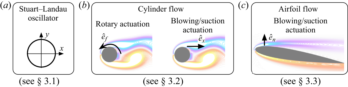
We demonstrate the phase-based flow-control strategy on three example systems as summarised in figure 2. First, we consider the SL oscillator, where the phase-sensitivity function can be computed analytically. We then demonstrate the phase-reduction analysis and optimal control on a canonical flow over a cylinder. Here, we explore two actuation strategies, one using rotary actuation and the other using momentum injection. Finally, we implement optimal phase control on a two-dimensional flow past an airfoil using blowing/suction actuation.
Summary of the examples considered in this work for optimal phase control: (a) SL oscillator, (b) unsteady flow over a cylinder at  $Re = 100$ with rotary and blowing/suction (
 $x$-direction) actuation, (c) unsteady two-dimensional flow over an airfoil at
 $Re = 1000$ and angle of attack of
 $\alpha = 9^\circ$ with blowing/suction actuation.

3.1. SL equation
We begin with a simple motivating example, given by the SL oscillator
 \begin{equation} \frac{\mathrm{d}A}{\mathrm{d}t} = {a_0 A - a_1 A |A|^2}+ \sigma\xi(t) + {Re}[f(t)], \end{equation}
where  $A(t) = x(t)+\textrm {i}y(t)$ is the complex amplitude,
 $f(t)$ is the forcing and
 ${\xi (t) = \xi _x(t) + \textrm {i}\xi _y(t)}$ is independent and identically distributed Gaussian white noise with unit variance and strength
 $\sigma$. For
 $\sigma >0$, the SL equation exhibits stochastic dynamics. We use a stochastic Runga–Kutta solver to integrate the dynamics (Kasdin Reference Kasdin1995). The SL equation was initially used to study the nonlinear instability of plane Poiseuille flow (Stuart Reference Stuart1960) and was later extended for weakly nonlinear stability analysis of cylinder wakes and open cavity flows (Sipp & Lebedev Reference Sipp and Lebedev2007). Bagheri (Reference Bagheri2013) showed that the leading Koopman eigenfunctions of the cylinder flow can also be constructed using the SL equation.
The well known Hopf normal form is given by
 $$\begin{gather} \frac{\textrm{d}\kern0.7pt x}{\textrm{d}t} = \mu x - \omega y - (x^2+y^2)(x - \beta y) + \sigma \xi_x(t) + f(t), \end{gather}$$
 $$\begin{gather}\frac{\textrm{d} y}{\textrm{d}t} = \omega y + \mu x - (x^2+y^2)(\beta x + y) + \sigma \xi_y(t), \end{gather}$$
where  $a_0 = \mu + \textrm {i} \omega$ and
 $a_1 = 1+\textrm {i}\beta$. Here,
 $f(t)$ is the forcing added in the
 $x$-direction (for phase control). We set
 $\mu = 0.1, \omega = 1$ and
 $\beta = 1$. The time step for numerical integration is
 $\Delta t = 0.01$. The radial amplitude is given by
 $r= \sqrt {x^2 + y^2}$. For the case with no noise, the radial amplitude is constant,
 $r(t) = r_0$, with a period of oscillation
 $T = 6.98$. The phase coordinate on the limit cycle is
 $\theta = \tan ^{-1}(y/x)$. The phase-sensitivity function for forcing in the
 $x$-direction can be constructed analytically (Moehlis Reference Moehlis2014) as
 \begin{equation} Z(\theta) = \frac{\beta}{\sqrt{\mu}}\cos\theta -\frac{1}{\sqrt{\mu}}\sin\theta. \end{equation}
This phase-sensitivity function only depends on the system parameters and the phase coordinate.
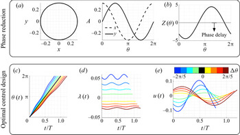
The baseline trajectories and the phase-sensitivity function for this example are shown in figure 3. A maximum phase delay is observed around  $\theta = {\rm \pi}/5$, while a maximum phase advance is observed around
 $\theta = 6{\rm \pi} /5$. We can also deduce its gradient analytically from (3.3). With this information, we are able to design an optimal phase controller, as described in § 2.3.
Overview of phase reduction and optimal phase control for the SL oscillator: (a) baseline trajectories; (b) analytical phase-sensitivity function and optimal control design for desired phase shifts of  $-2{\rm \pi} /5 \leqslant \Delta \theta \leqslant 2{\rm \pi} /5$; (c) phase-coordinate dynamics; (d) dynamics of the Lagrange multiplier; and (e) the optimal control input from the Euler–Lagrange equations.

We consider a range of phase shifts so that  $-2{\rm \pi} /5 \leqslant \Delta \theta \leqslant 2{\rm \pi} /5$. A phase advance of
 ${\Delta \theta = -2{\rm \pi} /5}$ corresponds to
 $T^*/T = 0.8$ and a phase delay of
 $\Delta \theta = 2{\rm \pi} /5$ corresponds to
 $T^*/T = 1.2$. The phase coordinate
 $\theta (t)$, corresponding Lagrange multiplier
 $\lambda (t)$ and the optimal control input
 $u(t)$ obtained by solving the associated Euler–Lagrange equations in (2.14a–c) are shown in figures 3(c), 3(d) and 3(e), respectively. The colour of the lines correspond to the varying values of desired phase shift. As described earlier, the initial condition
 $\lambda (0)$ is obtained by performing a shooting method. The converged initial conditions fall in the range
 $-0.026 \leqslant \lambda (0) \leqslant 0.0525$. For phase advance (negative phase shifts),
 $\lambda (t) > 0$, while for phase delays (positive phase shift),
 $\lambda (t) < 0$. The baseline phase is shown by the solid black line.
We also notice the correspondence between the phase-sensitivity function and the optimal control inputs  $u(t)$ in figures 3(b) and 3(e), respectively. The shape of the control input closely follows that of the phase-sensitivity function, especially for phase advance (negative phase shift). For phase delay (positive phase shift), the control input follows the opposite trend of the phase-sensitivity function. This is intuitive as the control input opposes any phase advances in the model by adding an opposite control force.
We implement the optimal control law  $f(t) = u(t)$ in the SL system in (3.2). Control simulations are performed with no noise (
 $\sigma = 0$) and with stochastic dynamics (
 $\sigma = 0.05$) for phase shifts of
 $\Delta \theta = \pm 2{\rm \pi} /5$. The control input
 $u(t)$, control trajectories
 $y(t)$ and the radial amplitude
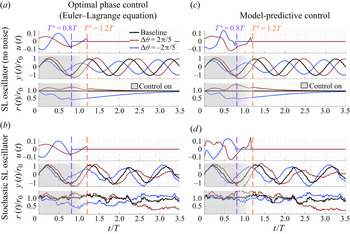
 $r(t) = \sqrt {x^2+y^2}$ for the baseline SL oscillator and the stochastic SL oscillator are shown in figures 4(a) and 4(b), respectively. For the baseline SL oscillator, the prescribed phase shift is achieved in the immediate transient (within
 $T^*$) for both the control cases corresponding to
 $\Delta \theta = \pm 2{\rm \pi} /5$. This phase shift is also observed in the asymptotic behaviour. For the stochastic system, shown in figure 4(b), the prescribed phase shifts are consistently achieved with control. This demonstrates the robustness of the control technique to stochastic disturbances. However, the phase shifts are not maintained asymptotically after the control is switched off. When the control is on, along with the phase shift, we also notice an amplitude modulation in the trajectories of
 $y(t)$. For phase delay, an increase in the amplitude is observed while for phase advance, a decrease in the amplitude is observed. These changes in the amplitude by performing optimal phase control are clearly visible in
 $r(t)$ as well.
Optimal phase control (using Euler–Lagrange equation) of the SL oscillator with (a) no noise ( $\sigma = 0$) and (b) stochastic dynamics
 $\sigma = 0.05$. Model predictive control of SL oscillator with (c) no noise (
 $\sigma = 0$) and (d) stochastic dynamics
 $\sigma = 0.05$. For each case, the control input
 $u(t)$, trajectory
 $y(t)$ and radial amplitude
 $r(t)$ are shown.

An alternative to the phase-control strategy already described is to use model predictive control (MPC) (Garcia, Prett & Morari Reference Garcia, Prett and Morari1989; Morari & Lee Reference Morari and Lee1999) based on the phase-reduced model. For MPC, a control problem is solved in real-time over a receding horizon subject to the imposed system constraints. The procedure for MPC-based control is described in Appendix A. For the SL oscillator, the prediction and control horizons are fixed at  $n_c = n_p = 8$, and we also fix
 $Q = 5, R = 1, R_{\Delta u} = 100$. Setting
 $R = 1$ penalises the control input
 $u$ in a similar manner to that discussed earlier for the energy-optimal phase-control strategy. A higher value of
 $R_{\Delta u}$ is necessary to ensure smooth control laws. The MPC control is switched on for time duration of
 $T^*$, after which the control is switched off. We emphasise that MPC is used for comparison of the control results from solving the Euler–Lagrange equations. The results using MPC are shown in figures 4(c) and 4(d). The MPC and energy-optimal control performance are remarkably similar, which is expected. The variation in the control inputs follow similar trends for both control cases and responses are almost identical. The associated cost function
 $\mathcal {C}[u(t)]$ for the Euler–Lagrange phase control from (2.13) for a phase shift of
 ${\Delta \theta = -2{\rm \pi} /5}$ is 0.0322 and for
 ${\Delta \theta = 2{\rm \pi} /5}$ is 0.0174. As the MPC cost function
 $\mathcal {J}[u(t)]$ described in Appendix A is different from
 $\mathcal {C}[u(t)]$, a fair comparison of the overall cost of control cannot be made. We find that the MPC control input cost
 $\int _0^{T^*} ||u||^2_{R_u} \,\textrm {d}t$ is slightly higher than that of the Euler–Lagrange control with 0.0373 for
 ${\Delta \theta = -2{\rm \pi} /5}$ and 0.0368 for
 ${\Delta \theta = 2{\rm \pi} /5}$. However, the total cost
 $\int _0^{T^*} \mathcal {J}[u(t)]\,\textrm {d}t$ is substantially higher, i.e. 2.36
 ${\Delta \theta = -2{\rm \pi} /5}$ and 1.73 for
 ${\Delta \theta = 2{\rm \pi} /5}$ resulting from state penalisation and enforcing a smooth control input.
The energy-optimal control strategy provides us with an intuition regarding the nature of the optimal control input by directly relating it to the phase-sensitivity function. The MPC does not provide such an intuitive connection, and obtaining an effective control law requires the tuning of state and input weights. The optimal phase-control strategy not only helps to advance and delay phases, but it also appropriately modulates the amplitude characteristics. In the following examples, we will see the implications of optimal phase control applied to unsteady fluid flows.
3.2. Laminar flow over a cylinder
We now demonstrate our phase-control approach on the canonical two-dimensional, incompressible flow past a circular cylinder at Reynolds number of  $Re = U_\infty d/\nu = 100$, where
 $U_\infty$ is the free stream velocity,
 $d$ is the cylinder diameter and
 $\nu$ is the kinematic viscosity. Direct numerical simulations are performed using the immersed-boundary projection method (Colonius & Taira Reference Colonius and Taira2008; Kajishima & Taira Reference Kajishima and Taira2017) with a computational grid extending over
 $(x/d,y/d) \in [-31,33] \times [-32, 32]$. A multi-domain technique is utilised with the smallest spatial resolution of
 $\Delta x/d = \Delta y/d = 0.02$. The simulation time step is
 $\Delta t = 0.005$. Details of the simulation and validation can be found in Colonius & Taira (Reference Colonius and Taira2008).
The baseline flow exhibits periodic vortex shedding in the cylinder wake with the shedding frequency of  $\omega _n = 2{\rm \pi} f_n U_\infty /d = 1.03$ (characteristic time
 $T = 2{\rm \pi} /\omega _n = 6.1$). In this flow, we will explore two different actuation strategies: first using rotary actuation (§ 3.2.1) and then using momentum injection (§ 3.2.2). Before we introduce perturbations for phase-reduction analysis or forcing input for phase-based control, we need to develop the actuation strategies.
3.2.1. Rotary actuation
In this section, we achieve phase control of the unsteady cylinder flow by rotating the cylinder as actuation. The phase-sensitivity function for this high-dimensional fluid flow cannot be deduced analytically. We follow the phase-reduction approach outlined in § 2.1 to construct the phase-sensitivity function. To introduce perturbations, we impulsively rotate the cylinder in the counterclockwise direction, as in (2.8).
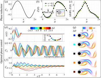
For reference, we show the baseline lift fluctuation over a period of oscillation in figure 5(a). Multiple direct numerical simulations are performed by introducing weak rotary perturbations ( $\epsilon = 0.1$) at various phases
 $\theta$. We then compute the asymptotic phase difference between the perturbed lift with respect to the baseline after
 $15$ periods of oscillation, resulting in the phase-sensitivity function
 $Z(\theta )$ using (2.10). We show the phase-sensitivity function for perturbation size of
 $\epsilon = 0.1$ in figure 5(b). For verification, we perform a similar analysis with a perturbation size of
 $\epsilon = 0.2$, and both sensitivity functions are nearly identical. Phase delay is generally observed for phases corresponding to
 $C_L >0$ and phase advance is observed for
 $C_L < 0$. The gradient of phase sensitivity
 ${\textrm {d} Z(\theta )}/{\textrm {d}\theta }$ is shown in figure 5(c). Larger gradients are observed at zero crossings of the lift curve.
Overview of phase reduction and optimal phase control for cylinder flow using rotary actuation: (a) lift coefficient ( $C_L$) of baseline cylinder flow with respect to the phase coordinate
 $\theta$, (b) phase-sensitivity function and (c) its gradient (right) for impulse perturbation introduced at an actuator located near the top separation point in the
 $\hat {e}_x$ direction, (d) energy-optimal control input required to shift the phase of oscillation (with associated cost function in inset), (e) lift and ( f) drag characteristics after application of forcing in direct numerical simulations, and (g) instantaneous flow fields immediately after control is turned off (
 $t = T^*$). The colour of the lines corresponds to the cases with desired phase shift
 $\Delta \theta$,
 $\Delta \theta = 0$ indicates baseline.

Using the phase-sensitivity function and its gradient, we are equipped to compute the optimal control input  $u(t)$ for phase alteration of unsteady flow oscillations. We consider a range of desired phase shifts
 $-2{\rm \pi} /5 \leqslant \Delta \theta \leqslant 2{\rm \pi} /5$, which correspond to
 $0.8 T \leqslant T^* \leqslant 1.2 T$. Solving the Euler–Lagrange equations in (2.14a–c), the control inputs for this range of phase shifts are shown in figure 5(d). For phase advance (negative phase shift) the control input follows a similar trend to that of the phase-sensitivity function, while for phase delay (positive phase shift) the control input follows the opposite trend. For positive phase shift, the control input opposes any phase advance in the sensitivity function. The inset in figure 5(d) shows the cost function
 $\mathcal {C}[u(t)]$ from (2.13) corresponding to the different phase shifts. As expected, lower cost is associated with smaller phase shifts. The cost for negative phase shifts is higher than for positive phase shifts, as the magnitude of the input is larger.
With the control input, we can determine the corresponding forcing to add to the Navier–Stokes equations, given by (2.11). We perform direct numerical simulations with the optimal forcing for each case, and the control forcing is switched off after  $t = T^*$. The lift coefficients for the controlled simulations are shown in figure 5(e). The baseline lift coefficient is shown in black. For all control cases, immediately after the application of control, the desired phase shift is achieved. Thus, the flow immediately locks on to the frequency prescribed within characteristic time (one period). The desired phase shift is sustained asymptotically after the control is switched off.
An important consequence of the optimal phase-control strategy is the effect on the amplitude of lift fluctuations in the immediate transient. We see that for positive phase shifts, the amplitude of lift fluctuation increases immediately after the application of control. For the negative phase shift, in the first oscillation cycle, the lift amplitude decreases with control. However, we observe a sharp rise in the lift fluctuation over the baseline in the second oscillation cycle. This increase in amplitude was not observed in the SL oscillator. Along with the lift coefficient, we also show the drag coefficient in figure 5( f). The drag coefficient decreases with positive phase shifts while it increases with negative phase shifts in the immediate transient. For positive phase shifts, a maximum drag reduction is achieved after the control is switched off. This is evidence that transient phase control is an effective means for both increasing lift and decreasing drag (Amitay & Glezer Reference Amitay and Glezer2002). Though not shown, the transient phase control may be repeated after the system reaches steady state, approximately six oscillation cycles later.
To understand the flow physics associated with the transient phase control, we analyse the instantaneous vorticity fields  $\boldsymbol {\omega }(\boldsymbol {x},t)$ at
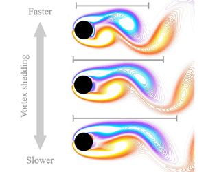
 $t= T^*$ for the different phase shifts, shown in figure 5(g). We can see that for negative phase shifts, the vortex shedding takes place earlier and the length of the shed vortex is shorter. The size of the shed vortex is proportional to the magnitude of the desired phase shift. An increase in the lift fluctuation is observed in the control cases of negative phase shifts after
 $t \geqslant T^*$. The other mechanism of increasing lift is to delay the vortex shedding as much as possible, which is seen in the positive phase-shift control cases. In these cases, the vortex shedding is delayed, resulting in an elongated vortical structure. This stabilises the recirculation region behind the cylinder and leads to a drag reduction as well. Note that the cost associated with shedding a vortex earlier is slightly larger. We argue that for positive phase shifts, the control principle is similar to that of direct-opposition control of vortices in the near wake, as discussed in the work of Siegel et al. (Reference Siegel, Cohen and McLaughlin2003) and Gerhard et al. (Reference Gerhard, Pastoor, King, Noack, Dillmann, Morzynski and Tadmor2003). In these works, direct-opposition control of wake structures with transversal oscillations of the cylinder enable the formation of elongated recirculation bubbles. Using a control law that opposes any phase advances in the phase-sensitivity function leads directly to control of vortices in the near wake.
3.2.2. Momentum injection
Next, we investigate the optimal phase-control technique for another actuation input based on momentum injection, where we add a localised force to the Navier–Stokes equation to copy a blowing/suction type actuator. The spatial profile of the actuator is a Dirac delta in space, approximated using a three-cell discrete delta function (Roma, Peskin & Berger Reference Roma, Peskin and Berger1999). The actuation is introduced at the time-averaged separation point  $\boldsymbol {x}_s$ on the upper surface of the cylinder, at an angle of
 $58.4^\circ$ from the aft end and positioned at
 $3\Delta x$ from the cylinder surface. The actuation is prescribed in the
 $x$-direction. While there is flexibility in choosing the actuation for the proposed control method, some actuation configurations may be more effective for the controlling phase (Bhattacharjee et al. Reference Bhattacharjee, Hemati, Klose and Jacobs2018; Taira & Nakao Reference Taira and Nakao2018).
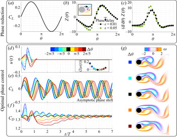
For reference, the baseline lift is shown in figure 6(a). Again, the phase-sensitivity function  $Z(\theta )$ is obtained from impulsive perturbations, as shown in figure 6(b). The analysis is performed for perturbation amplitudes of
 $\epsilon = 0.01$ and
 $0.05$. The phase-sensitivity functions are similar for different perturbation sizes, except near
 $\theta = 3{\rm \pi} /5$. Compared to the rotary-control case, the phase-sensitivity function has a larger magnitude at most characteristic phases. This shows that the flow is more responsive to momentum injection than rotary control. The gradient of the phase-sensitivity function is highest around
 $\theta = {\rm \pi}$, as seen in figure 6(c).
Overview of phase reduction and optimal phase control for cylinder flow using a momentum injection: (a) lift coefficient ( $C_L$) of baseline cylinder flow with respect to the phase coordinate
 $\theta$, (b) phase-sensitivity function and (c) its gradient (right) for impulse perturbation introduced at an actuator located near the top separation point in the
 $\hat {e}_x$ direction, (d) the energy-optimal control input required to shift the phase of oscillation (with associated cost function in inset), (e) lift and ( f) drag characteristics after application of forcing in direct numerical simulations, and (g) instantaneous flow fields immediately after control is turned off (
 $t = T^*$). The colour of the lines corresponds to the cases with desired phase shift
 $\Delta \theta$, with
 $\Delta \theta = 0$ indicating the baseline.

The phase-control inputs to achieve the desired phase shifts using momentum injection are shown in figure 6(d). As with rotary actuation, the cost function is larger for negative phase shifts (shown in inset). However, the cost of momentum injection is an order of magnitude lower. This is expected because of the increased phase sensitivity in the momentum injection case. We can also compute the actuation cost with the steady and unsteady momentum coefficients given by
 \begin{equation} \bar{C}_\mu = \frac{\rho u_{jet}^2 \sigma}{\frac{1}{2}\rho U_\infty^2 d},\quad {C}^\prime_\mu = \frac{\rho u_{rms}^2 \sigma}{\frac{1}{2}\rho U_\infty^2 d}, \end{equation}
respectively, where  $\sigma$ is the actuator width, given by the grid spacing
 $\sigma = \Delta x$. The characteristic velocities
 $u_{jet}$ and
 $u_{rms}$ are computed with companion simulations by setting the free-stream velocity to be zero (Munday & Taira Reference Munday and Taira2013). The steady and unsteady coefficients of momentum for
 $\Delta \theta = -2{\rm \pi} /5$ are
 $\bar {C}_\mu = 0.0078$ and
 $C^\prime _\mu = 0.0125$, respectively. For
 $\Delta \theta = 2{\rm \pi} /5$,
 $\bar {C}_\mu = 0.006$ and
 $C^\prime _\mu = 0.01$.
Incorporating the forcing input in the Navier–Stokes equations, we perform direct numerical simulations for the variously desired phase shifts. The time history of the lift and drag coefficients in the controlled simulations are shown in figures 6(e) and 6( f), respectively. We see similar control performance with respect to the transient phase shift, lift fluctuation and asymptotic phase shift compared with the rotary actuation case. However, the performance in drag differs slightly. When the control is on, the drag both increases and decreases with respect to the baseline. When the control is off, the drag coefficient decreases for positive phase shifts and increases slightly for negative phase shifts. This is consistent with the results from rotary actuation. The (controlled) instantaneous vorticity fields at  $t = T^*$ are shown in figure 6(g). The characteristic flow physics for the control based on momentum injection is almost identical to that of rotary actuation. This shows the consistency of the optimal phase-control approach in terms of altering the vortex shedding behaviour for different actuation strategies.
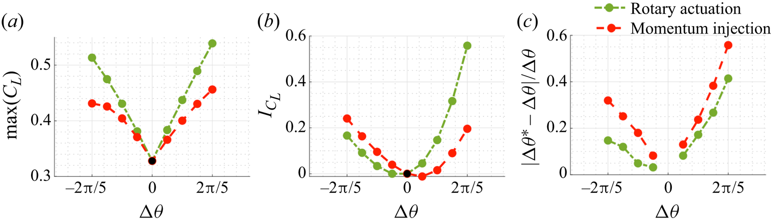
We now compare key features of interest for both rotary actuation and momentum injection. In particular, we investigate the maximum lift coefficient, lift impulse and the error in asymptotic phase shift with optimal phase control, as shown in figures 7(a), 7(b) and 7(c), respectively. Lift impulse is the area under the lift-time curve (Williams et al. Reference Williams, Tadmor, Colonius, Kerstens, Quach and Buntain2009), demonstrating the overall benefit of control in terms of lift enhancement. With an increase in the phase shift, the maximum lift increases. With larger phase shifts, the benefit in lift enhancement increases dramatically. However, because of the considerable amplitude variation, the error in asymptotic phase shift increases with phase shift. This is expected as the optimal control input is based on infinitesimal phase-sensitivity functions and larger control amplitudes introduce nonlinear effects. The phase-control performance of rotary control is superior to that of momentum injection from an aerodynamic view point. However, as mentioned before, the cost associated with rotary control is an order of magnitude higher.
Comparison of control performance for rotary actuation and momentum injection: (a) maximum lift coefficient, (b) lift impulse and (c) error in asymptotic phase shift for varying desired phase shifts.

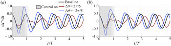
Amitay & Glezer (Reference Amitay and Glezer2002, Reference Amitay and Glezer2006) analysed transients associated with flow reattachment and separation using pulsed amplitude modulation of a synthetic jet actuator. They observed that shedding of large vortices and momentary increase in circulation were crucial in terms of achieving the transient flow attachment. These enhancements were accentuated with actuation frequency close to the natural frequency of the flow (Amitay & Glezer Reference Amitay and Glezer2006; Colonius & Williams Reference Colonius and Williams2011). We similarly investigate flow transients in terms of the rate of change of circulation to characterise the effect of control given by
 \begin{equation} \frac{\mathrm{d}\varGamma}{\mathrm{d}t} = \int_{x/d = \text{const}} \omega(\boldsymbol{x},t) \boldsymbol{q}(\boldsymbol{x},t)\boldsymbol{\cdot} \hat{\boldsymbol{e}}_x \,\mathrm{d} y, \end{equation}
where  $\boldsymbol {q}$ is the velocity field and
 $\omega$ is the vorticity. We compute the vorticity flux at
 $x/d = 1.2$. The rate of change of circulation with time, for both rotary actuation and momentum injection, are shown in figure 8(a,b) for
 $\Delta \theta = -2{\rm \pi} /5$ and
 $2{\rm \pi} /5$. The trends are similar to the variation in the lift coefficient. The instantaneous vorticity flux for positive phase shifts is slightly greater than that of the baseline in the initial oscillation leading to an immediate increase in lift coefficient. The rate of change of circulation with time increases dramatically towards the end of the control forcing for the negative phase shift. This time corresponds to the vortex pinch-off, i.e. when the vortex is shed. The increase in flux is larger for the rotary actuation, leading to higher control performance compared to that of momentum injection.
Vorticity flux comparison with respect to the baseline for (a) rotary control and (b) momentum injection.

3.3. Flow over an airfoil
Finally, we demonstrate the optimal phase-control approach on a two-dimensional, incompressible flow over a NACA0012 airfoil at an angle of attack  $\alpha = 9^\circ$ with a chord-based Reynolds number
 $Re = 1000$. This example is chosen to demonstrate the advanced capabilities of the phase-based control approach to enhance aerodynamic characteristics of wings in unsteady flow conditions.
The immersed-boundary projection method is used for direct numerical simulation (Colonius & Taira Reference Colonius and Taira2008). Five nested domains are used, with an outermost domain of  $-16 \leqslant x/c \leqslant 16, -16 \leqslant y/c \leqslant 16$ and an inner grid resolution of
 $\Delta x = 0.0055$, where
 $c$ is the chord length. The integration time step is
 $\Delta t = 0.001$. The baseline lift coefficient fluctuation is shown in figure 9(a). The mean lift force is
 $\bar {C}_L = 0.394$ and the oscillation frequency is
 $\omega _n = 2{\rm \pi} f_nU/c = 7.17$, which corresponds to a characteristic time of
 $T = 2{\rm \pi} /\omega _n$. There are three fundamental differences in this high-dimensional flow example compared to the previous cylinder flow example: (i) the baseline mean lift force is non-zero, (ii) the harmonics of the natural shedding frequency are stronger and can be observed in the baseline lift oscillation, and (iii) the flow exhibits both leading-edge and trailing-edge separation.
Overview of phase reduction and optimal phase control for flow over an airfoil using momentum injection: (a) lift coefficient ( $C_L$) of baseline cylinder flow with respect to the phase coordinate
 $\theta$, (b) phase-sensitivity function and (c) its gradient (right) for impulse perturbation introduced at an actuator located near the top separation point in the
 $\hat {e}_x$ direction, (d) energy-optimal control input required to shift the phase of oscillation (with associated cost function in inset), (e) lift characteristics after application of forcing in direct numerical simulations for negative and positive phase shifts (shown separately) and ( f) instantaneous flow fields after control is turned off (
 $t = 2T^*$). The colour of the lines corresponds to the cases with desired phase shift
 $\Delta \theta$,
 $\Delta \theta = 0$ indicates baseline. For visual clarity, the fluctuations in the controlled lift trajectories are shown as shaded areas relative to the baseline lift coefficient.

For phase reduction and optimal phase control, we use a wall-normal momentum injection modelled by a localised force added near the average separation point. We then perform the impulse-response analysis at  $25$ characteristic phases
 $\theta$. The difference between the perturbed trajectories and the baseline fluctuations after
 $20$ time periods of oscillation is assessed to compute the phase-sensitivity function, as shown in figure 9(b). After introducing the perturbation, the flow takes more oscillations to reach a steady state compared to the cylinder flow. The amplitude of the perturbation is
 $\epsilon = 0.0005$. The magnitude of the phase-sensitivity function is larger compared to both actuation cases for the cylinder flow example. The maximum phase-advance sensitivity is observed at the phase corresponding to minimum lift coefficient. Phase-delay sensitivity is largest at phases corresponding to a larger lift coefficient. Surprisingly, the phase-sensitivity function has a sinusoidal shape, even for this highly complex flow. The corresponding gradient is shown in figure 9(c). The optimal control inputs for a desired phase shift
 $-2{\rm \pi} /5 \leqslant \Delta \theta \leqslant 2{\rm \pi} /5$ are shown in figure 9(d). The associated cost of control (shown in the inset) is lower than the corresponding cost of momentum injection for the cylinder flow example. This is expected as the magnitude of the phase-sensitivity function for the airfoil flow is larger. The steady and unsteady coefficients of momentum for
 $\Delta \theta = -2{\rm \pi} /5$ are
 $\bar {C}_\mu = 0.01$ and
 $C^\prime _\mu = 0.0132$, respectively. For
 $\Delta \theta = 2{\rm \pi} /5$,
 $\bar {C}_\mu = 0.01$ and
 $C^\prime _\mu = 0.01$.
After applying the optimal forcing input to the Navier–Stokes equations and performing direct numerical simulations, we examine the fluctuations in the lift coefficient compared with the baseline for all cases in figure 9(e). To highlight the variation with respect to the baseline, we separate the lift fluctuation for negative phase shifts and positive phase shifts. We also colour the increments in the fluctuation to further emphasise the changes with control. Similarly to the cylinder flow example, we achieve an immediate increase in lift for the positive phase-shift cases. The transient phase shift is exactly as prescribed, indicating that immediate lock-on is obtained even for this complex flow. We also see that lift fluctuations are higher than the baseline for all cases for a number of oscillation cycles, even after the control is switched off. Note that although there are distinct harmonic oscillations in the baseline lift, when control is applied, these harmonics are suppressed until the flow evolves for more than four convective units. The work of Joe, Colonius & MacMynowski (Reference Joe, Colonius and MacMynowski2011) on an inclined flat plate showed that larger ranges of negative phase shift in the control signal contributed to lift enhancement, while sharp decreases in enhancement at positive phase-shift regimes were observed. There is a preference for negative phase shifts for larger lift enhancement. While not shown, the drag force decreases during control for both positive and negative phase shifts. When the control is switched off, the drag force increases owing to the nonlinear interaction with the trailing-edge vortices, and so breaks the flow stabilisation in the wake.
On observing the characteristic vorticity flow fields associated with the control cases in figure 9( f), we see that a leading-edge vortex (Wang & Eldredge Reference Wang and Eldredge2013; Eldredge & Jones Reference Eldredge and Jones2019) forms earlier for the controlled flow with negative phase shifts. For positive phase shifts, the roll-up process of the leading-edge vortex is delayed, resulting in wake elongation. In the negative phase-shift cases, the interaction of the shed leading-edge vortex with the trailing-edge vortex results in high lift after the control is switched off. These results are consistent with the findings of Darabi & Wygnanski (Reference Darabi and Wygnanski2004) and Colonius & Williams (Reference Colonius and Williams2011). Thus, with optimal phase control, we can control the timing of vortex shedding. We also highlight the maximum lift force and corresponding lift impulse in figures 10(a) and 10(b), respectively. We can clearly see that negative phase shifts are preferred for maximum lift and lift impulse. A clear benefit in lift impulse for positive phase shifts is only observed for  $\Delta \theta >{\rm \pi} /10$. Thus, optimal phase control is an effective way of increasing transient aerodynamic performance.
Evaluation of control performance: (a) maximum lift coefficient and (b) lift impulse for varying phase shifts.

4. Conclusion
We have developed a control strategy to modify the phase of nonlinear, periodic fluid flows. Our control strategy combines phase-amplitude reduction and optimal phase-based control techniques for high-dimensional unsteady fluid flows. The phase-reduction technique describes the phase dynamics of unsteady fluid flows via a phase-sensitivity function, complementing Floquet theory. Importantly, we show how this description can be used for effective flow control, demonstrating how it can be used to modify vortex dynamics in the near wake of bluff-body flows, and on time scales commensurate with the period of vortex shedding. We consider several example systems, including the SL oscillator, the canonical fluid flow past a cylinder and a highly complex fluid flow past an airfoil, illustrating the use of this approach for practical tailoring of aerodynamic responses. Our control strategy requires only measurements of physically attainable observables, such as lift and drag, and does not require high-dimensional data.
We demonstrate the performance of this phase-based control approach for two flow systems, the canonical flow over a cylinder and flow over an airfoil. In each system, our control law is only active for approximately one oscillation cycle, and is highly effective in modifying the phase of the flow to a desired phase shift. We explore the optimal phase-control strategy for a range of prescribed phase shifts with respective to the baseline oscillation. Interestingly, two separate mechanisms are exploited to achieve lift enhancement for negative and positive phase shifts. For negative phase shifts, the vortex formation process and shedding are accelerated. In contrast, for positive phase shifts, vortex structures in the wake are elongated and we observe an immediate increase in lift. As the wake is elongated and in turn stabilised, we also achieve a transient drag reduction. Investigating the relationship between the control forcing and the phase-sensitivity function, we observe that for positive phase shifts the control principle is similar to performing direct-opposition control to restrict the shedding of vortex structures.
We propose two control approaches to rapidly and efficiently alter the phase dynamics of unsteady fluid flows; comparing these two approaches illuminates some interesting trade-offs. In the first approach, we solve an offline optimisation problem using the Euler–Lagrange equations and then design the optimal forcing. Because this solution is tied directly to the phase-sensitivity function, it is simple, effective and has an intuitive interpretation. The second approach involves real-time feedback control using MPC. For the simple SL oscillator, the two approaches are remarkably similar. However, the associated cost with Euler–Lagrange equations is relatively lower for similar performance.
The main focus of the present work has been to control the phase of periodic vortex shedding in unsteady fluid flows. The fundamental limitation is that the method only applies to limit-cycle systems. However, there is tremendous scope to build on this analysis for future work. Both phase and amplitude reduction are necessary to extend the control approach to systems with unstable fixed points (Wilson Reference Wilson2020). The phase-amplitude reduction analysis could be combined with cluster-based approaches (Kaiser et al. Reference Kaiser, Noack, Cordier, Spohn, Segond, Abel, Daviller and Niven2014; Nair et al. Reference Nair, Yeh, Kaiser, Noack, Brunton and Taira2019) to improve its applicability to aperiodic flows. This may enable us to stabilise unstable orbits as well as promote synchronisation in quasi-periodic systems. Further work needs to be done in representing the phase of more complex multi-modal observables, such as those found in fluid–structure interactions. A thorough assessment of the underlying influence of controllability and observability on the effectiveness of the flow-control strategy is also needed. The present methodology to compute the optimal actuation input  $u$ can be further refined by combining with adjoint-based methods from Giannetti et al. (Reference Giannetti, Camarri and Citro2019) to extract spatial forcing
 $\boldsymbol {h}(\boldsymbol {x})$. Finally, it may be possible to extend the optimisation procedure described previously to a longer horizon, which will potentially uncover more favourable control laws.
Acknowledgements
We thank Professor H. Nakao, Dr C.-A. Yeh and B. Monga for valuable discussions.
Funding
A.G.N. acknowledges support from UNR VPRI startup grant PG19679. K.T. acknowledges support from the Air Force Office of Scientific Research (FA9550-18-1-0040). B.W.B. acknowledges support from the Air Force Office of Scientific Research (FA9550-18-1-0114) and the Air Force Research Lab (FA8651-16-1-0003). S.L.B. acknowledges support from the Army Research Office (W911NF-17-1-0306) and the Air Force Office of Scientific Research (FA9550-18-1-0200). B.W.B. and S.L.B. acknowledge support from the Air Force Office of Scientific Research (FA9550-19-1-0386).
Declaration of interests
The authors report no conflict of interest.
Data availability statement
The optimal phase-control code and phase-sensitivity data for the examples in this work are available at https://github.com/nairaditya/Phase-control-fluid-flow.
Appendix A. MPC
Here, we elaborate on MPC (Garcia et al. Reference Garcia, Prett and Morari1989) for optimal phase control. We can use MPC to perform real-time feedback control, can incorporate constraints and has been shown to be robust to noisy measurement input. A schematic for MPC is shown in figure 11(a). For a problem of interest, there are four key components for MPC: (i) the dynamical system (plant) on which control is added (in the case of fluid flows – this would be the Navier–Stokes equation, given by (2.2a,b)); (ii) the model used for prediction of the state (or observable); (iii) desired reference state to be achieved with control; and (iv) the control optimisation algorithm used to deduce the real-time optimal-control law. The optimal-control problem is solved over a receding horizon to determine the next control input. The optimisation is repeated at each time step and the control law is updated, as shown in figure 11(b).
(a) Schematic of the MPC structure and (b) receding horizon framework (adapted from Kaiser, Kutz & Brunton Reference Kaiser, Kutz and Brunton2018).

In the work of Kaiser et al. (Reference Kaiser, Kutz and Brunton2018), MPC was combined with several models based on dynamic mode decomposition (Schmid Reference Schmid2010), neural networks (Hornik, Stinchcombe & White Reference Hornik, Stinchcombe and White1989) and sparse identification of nonlinear dynamics (Brunton, Proctor & Kutz Reference Brunton, Proctor and Kutz2016). Here, for prediction of the state, we use the phase-reduced model given by (2.12). For simplicity, at time  $t_j$,
 $r_j$ is the reference state,
 $\theta _j$ is the phase coordinate and
 $u_j$ is the control input. Note that for unsteady fluid flows, the forcing is described by (2.11). For phase-based control, the reference
 $r$ should be
 $T^*$ periodic for a desired phase shift of
 $\Delta \theta = \omega _n(T^* - T)$; thus
 $r_j = 2{\rm \pi} t_j/T^*$. The output of the phase-reduced model is
 $\hat {\theta }$ and the control-optimiser output is
 $\hat {u}$. As shown in figure 11(b), the prediction and optimisation horizons are
 $n_p$ and
 $n_c$ time steps, respectively. At each step, the control optimisation identifies a sequence of control inputs
 $\hat {u} = \{\hat {u}_{j+1}, \hat {u}_{j+2}, \ldots ,\hat {u}_{j+n_c}\}$ based on predicted phases
 $\hat {\theta } = \{\hat {\theta }_{j+1}, \hat {\theta }_{j+2}, \ldots ,\hat {\theta }_{j+n_p}\}$, after which
 $u_j = \hat {u}_{j+1}$ is applied to the plant, and then the procedure is repeated.
The MPC optimisation (Kaiser et al. Reference Kaiser, Kutz and Brunton2018) at each time step is given by
 \begin{equation} \min\limits_{{\hat{u}}} \mathcal{J}= \min\limits_{{\hat{u}}} \sum\limits_{{k=0}}^{n_p} ||\hat{\theta}_{j+k} - r_{j+k}||^2_{Q} + \sum_{{k=1}}^{n_c} (||\hat{u}_{j+k}||^2_{R_u} + ||\Delta \hat{u}_{j+k}||^2_{R} ), \end{equation}
subject to the constraints  $\hat {u}_{min} \leqslant \hat {u}_k \leqslant \hat {u}_{max}$ and
 $\Delta \hat {u}_{min} \leqslant \Delta \hat {u}_k \leqslant \Delta \hat {u}_{max}$. Here,
 $\Delta \hat {u}_k = \hat {u}_k - \hat {u}_{k-1}$ is the input rate. We penalise the phase coordinate, control input and its rate. In addition, for each term, a weighted norm is computed
 $||x||_Q = x^T Q x$. The weights are chosen to be positive semi-definite.