


1. Introduction
It remains our longstanding claim that turbulence can be meaningfully understood, modelled and controlled via coherent structures – the underlying large-scale vortical structures – also the so-called ‘order within disorder’, which dominate the dynamics of turbulent flows and presumably the only vehicle via which turbulence phenomena and noise generation can be controlled – leading to the claim: ‘no coherent structures, no control’ (Hussain Reference Hussain1986). Prior studies of vortex dynamics, such as vortex–turbulence interaction (Melander & Hussain Reference Melander and Hussain1993; Pradeep & Hussain Reference Pradeep and Hussain2010) and vortex reconnection (Melander & Hussain Reference Melander and Hussain1988; Hussain & Duraisamy Reference Hussain and Duraisamy2011), strongly suggest that coherent structures are usually polarized (i.e. with axial flows). Recently, Goto and co-workers (Goto, Saito & Kawahara Reference Goto, Saito and Kawahara2017; Motoori & Goto Reference Motoori and Goto2019) also showed that turbulent flows consist of a hierarchy of anti-parallel pairs of polarized vortex tubes, which are spawned by stretching in strain fields around stronger vortices. The study of the dynamics and interaction of polarized vortical structures is, therefore, an essential avenue for understanding turbulent flows and their modelling and control.
Although not as extensive as in the unpolarized case, considerable works have been done on polarized vortical dynamics, most of which are focused on identifying and describing their instabilities. Temporal linear normal-mode stability analysis showed that strong inviscid helical instabilities are present for an idealized vortex column (e.g. Batchelor vortex, which is a Lamb–Oseen vortex with a Gaussian axial velocity profile) with swirl number (defined as the ratio of peak azimuthal to axial velocities) less than 1.5 (Stewartson & Brown Reference Stewartson and Brown1985; Mayer & Powell Reference Mayer and Powell1992). These are the only unstable modes when the swirl number is zero, which corresponds to a non-rotating Gaussian jet, and undergo the highest growth when the swirl number is around  $0.5$, and are ultimately stabilized for high swirls. Subsequently, transient growth of perturbations has been studied but appears to be important only in cases when the normal-mode instabilities are relatively weak, such as in moderate- to high-swirl flows (Heaton & Peake Reference Heaton and Peake2007). Another important type of instabilities, referred to as cooperative instabilities, occurs in systems of two or more vortices and is caused by the straining field induced on each vortex by the others. Cooperative instabilities can be further classified into long-wave (Crow Reference Crow1970) and short-wave (Moore & Saffman Reference Moore and Saffman1975) instabilities, and both can be explained as a resonance mechanism involving a pair of Kelvin waves. Lacaze, Ryan & Le Dizes (Reference Lacaze, Ryan and Le Dizes2007) analysed the elliptic instability of a Batchelor vortex and found that the resonant Kelvin modes
 $m=1$ and
 $m = -1$, which are the most unstable in the absence of axial flow, become damped as the axial flow is increased. Instead, other instability modes corresponding to resonance of two Kelvin modes of azimuthal wavenumbers
 $m$ and
 $m+2$ are shown to become progressively unstable for increasing axial flow. Among them, the
 $(-2, 0)$ mode is the most unstable for weak axial flow cases. Following that work, Roy et al. (Reference Roy, Schaeffer, Le Dizès and Thompson2008) conducted linear instability analysis of co-rotating vortices with axial flows. As the axial flow is increased, different instability modes are observed as a combination of resonating Kelvin modes of azimuthal wavenumbers
 $m$ and
 $m+2$ within each vortex – akin to the finding for the counter-rotating case.
Beyond the works on the vortex column, numerous others have focused on the vortex ring with core axial flows – referred to as swirling vortex ring (Moffatt Reference Moffatt1988; Grauer & Sideris Reference Grauer and Sideris1991). For example, Virk, Melander & Hussain (Reference Virk, Melander and Hussain1994) studied the dynamics of an isolated polarized vortex ring and found that the evolutionary dynamics is quite different from that of the unpolarized case. In particular, the propagation velocity decreases monotonically as the degree of initial polarization increases. A similar study was performed by Cheng, Lou & Lim (Reference Cheng, Lou and Lim2010), who confirmed that increasing the swirl of the ring results in the vortex ring slowing down or even travelling backward! They also found that, for a sufficiently strong swirl, parts of the ring are shed into the wake as vortex loops or hairpin vortices, which can further undergo vortex reconnection with themselves. Naitoh et al. (Reference Naitoh, Okura, Gotoh and Kato2014) experimentally studied the laminar swirling vortex ring and observed that axial flow in the ring could reduce the amplification rate of the azimuthal wavy deformation – thus, the ring can better preserve its structure and travel a longer distance. Linear instability analysis by Gargan-Shingles, Rudman & Ryan (Reference Gargan-Shingles, Rudman and Ryan2016) further showed that the addition of swirl alters the instability mode of the vortex ring, suppressing the development of the  $(-1,+1)$ mode and enhancing the
 $(-2,0)$ and
 $(-3,-1)$ modes, similar to those observed for vortex pairs. Recently, Hattori, Blanco-Rodríguez & Le Dizès (Reference Hattori, Blanco-Rodríguez and Le Dizès2019) performed direct numerical simulation (DNS) of the linear instability of a swirling vortex ring and found that the vortex ring can undergo curvature instability, as analytically predicted by Blanco-Rodríguez & Le Dizès (Reference Blanco-Rodríguez and Le Dizès2017) for a curved Batchelor vortex.
An important quantity related to the dynamics of polarized vortices is helicity (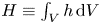 $H\equiv \int _V h\,\mathrm {d}V$ with
 $h=\boldsymbol {u}\boldsymbol {\cdot } \boldsymbol {\omega }$ being the helicity density and
 $V$ the entire flow domain), which measures the degree to which vortex lines embedded in a fluid system wind around each other (Moffatt Reference Moffatt1969; Scheeler et al. Reference Scheeler, van Rees, Kedia, Kleckner and Irvine2017). In addition to energy, helicity is also conserved in ideal fluids. Note that, in the Navier–Stokes (N–S) equations, the nonlinear Lamb vector term
 $\boldsymbol {\omega }\times \boldsymbol {u}$ is responsible for cascade from larger to smaller scales (Wu, Ma & Zhou Reference Wu, Ma and Zhou2007). Wherever
 $h$ is large, the Lamb vector is trivially small because of the trigonometric identity
 \begin{equation} |\boldsymbol{u}\boldsymbol{\cdot}\boldsymbol{\omega}|^{2}+|\boldsymbol{\omega}\times \boldsymbol{u}|^{2}=|\boldsymbol{u}|^{2}|\boldsymbol{\omega}|^{2}. \end{equation}
It therefore follows that helical (or polarized) structures will have low dissipation and can be expected to be long-lived, as a result of Beltramization ( $\boldsymbol {u}||\boldsymbol {\omega }$). For a vortex tube with finite core size, helicity can be further decomposed into three topological forms: link, writhe and twist (Moffatt & Ricca Reference Moffatt and Ricca1995; Scheeler et al. Reference Scheeler, van Rees, Kedia, Kleckner and Irvine2017). In order to understand the role of helicity in vortex dynamics, the evolution of knotted or linked vortices has been extensively studied. For example, Kida & Takaoka (Reference Kida and Takaoka1987) conducted the first DNS study of trefoil knotted vortices at a vortex Reynolds number
 $Re$
 $(\equiv \varGamma _0/\nu )=1200$ and observed that helicity continuously decreases during reconnection. Recently, Scheeler et al. (Reference Scheeler, Kleckner, Proment, Kindlmann and Irvine2014) experimentally constructed a trefoil knotted vortex in water and found that helicity is surprisingly conserved during reconnection: vortex knots untie, but during this process, they create helical-like coils with the same total helicity. Kerr (Reference Kerr2018b) numerically investigated the evolution of perturbed trefoil knotted vortices and confirmed that the total helicity is conserved before reconnection, followed by a progressive and steady decay after reconnection. Zhao et al. (Reference Zhao, Yu, Chapelier and Scalo2021) performed DNS of the trefoil knotted vortex up to
 $Re=6000$ and observed that helicity can experience a sudden jump during and after reconnection, particularly at high
 $Re$. The increase of helicity should be attributed to asymmetric reconnection, but the detailed physical mechanism still remains rather elusive. As two interacting vortices with arbitrary orientations tend to become anti-parallel when they approach, it might be beneficial to study reconnection of the anti-parallel configuration to shed light on this enigma.
In contrast to the vast literature on instability/dynamics of an isolated polarized vortex, interactions, especially reconnection, of polarized vortices are less studied. van Rees, Hussain & Koumoutsakos (Reference van Rees, Hussain and Koumoutsakos2012) performed reconnection of two anti-parallel co-polarized vortex tubes and compared that with the unpolarized case at  $Re=10\,000$. They found that the presence of axial flow significantly alters the reconnection process, and the energy spectrum exhibits a
 $-7/3$ slope, different from the typical
 $-5/3$ slope for the unpolarized case. McGavin & Pontin (Reference McGavin and Pontin2019) addressed the topology of vortex tube reconnection for both co- and counter-polarization cases at a relatively low
 $Re$ (i.e. 800). They observed that the topology evolution is quite different between these two cases. Similar to the unpolarized case, the reconnection is locally two-dimensional for counter-polarized cases; however, it becomes fully three-dimensional for counter-polarized cases, namely vortex lines reconnect at a finite angle.
Despite its significant relevance to real flows, the effect of polarization on vortex reconnection still remains poorly understood. In the present work, we perform a systematic study of reconnection of polarized vortices by considering a wide range of Reynolds numbers and polarization strengths. Our main objective is to provide a better understanding of how the presence of axial flows affects the various aspects of the reconnection process. In addition, we also want to further shed light on how helicity, particularly helicity density, alters the energy cascade. The rest of the paper is organized as follows. In the following section, we first discuss the details of the initial configuration and numerical set-up. The reconnection results for the counter- and co-polarized cases are presented in §§ 3 and 4, respectively. The Reynolds number effect and polarization effect on energy and helicity cascade are discussed in § 5, and, finally, conclusions are drawn in § 6.
2. Computational methods and initial configuration
To focus on the basic mechanism of reconnection, we adopt a simple configuration similar to that used in Melander & Hussain (Reference Melander and Hussain1988) and van Rees et al. (Reference van Rees, Hussain and Koumoutsakos2012). The initial condition consists of two anti-parallel vortices with a sinusoidal perturbation. Each vortex has a circular cross-section with
 \begin{equation} \omega(r)= \begin{cases} \omega_0[1-f(r/r_c)], & \text{if }r\geqslant r_c\\ 0, & \text{otherwise}, \end{cases} \end{equation}
where  $f(r)=\exp [-Kr^{-1}\exp [1/(r-1)]]$,
 $K=1/2\exp (2)\log (2)$,
 $r_c$ is the core size and
 $\omega _0$ is the initial maximum axial vorticity.
The axial flow imposed initially on the tubes is based on an axisymmetric velocity profile (similar to the vorticity profile):
 \begin{equation} u_z(r)= \begin{cases} u_0[1-f(r/r_c)], & \text{if }r\geqslant r_c\\ 0, & \text{otherwise}, \end{cases} \end{equation}
where  $u_0$ is the initial maximum axial velocity.
The vorticity field obtained by adding the component due to axial flow is sinusoidally perturbed. For the vortex tube in the negative half of the  $x$ plane, the core location is
 $\boldsymbol {r}=[x_c+p\cos \alpha f(z), y_c+p \sin \alpha f(z)]$ with
 $(x_c,y_c)=(-0.81,0), \alpha =60^{\circ }$,
 $r_c=2/3$,
 $p=0.2$ and
 $f(z)=\cos (z)$. Note that the initial condition was designed to have the two sinusoidal vortices initially inclined to each other and near to each other so that the vortex peaks will immediately collide with each other via self-induction before they get to diffuse too much and hence readily commence reconnection. After the perturbation is applied, the vorticity field
 $\boldsymbol {\omega }_{\boldsymbol {in}}$ is no longer divergence-free, and a solenoidal reprojection is applied (Melander & Hussain Reference Melander and Hussain1988; Shelley, Meiron & Orszag Reference Shelley, Meiron and Orszag1993). In particular, a modified initial velocity field
 $\boldsymbol {u}$ is obtained by inverting the following equation:
 \begin{equation} \nabla^{2}\boldsymbol{u}=\boldsymbol{\nabla}\times\boldsymbol{\omega}_{\boldsymbol{in}}. \end{equation}
Then, the corresponding initial vorticity fields can be obtained by following the definition  $\boldsymbol {\omega }=\boldsymbol {\nabla }\times \boldsymbol {u}$.
The DNS of the incompressible N–S equations in the velocity–vorticity form is carried out using a Fourier pseudospectral algorithm in a periodic domain with dimensions  $(2{\rm \pi} )^{3}$ (Pradeep & Hussain Reference Pradeep and Hussain2004; Yao & Hussain Reference Yao and Hussain2020b). Time integration is carried out with an explicit third-order Runge–Kutta scheme, while the viscous term is treated exactly with the integrating factor technique (Canuto et al. Reference Canuto, Hussaini, Quarteroni and Thomas2012). Following previous studies (Hussain & Duraisamy Reference Hussain and Duraisamy2011; Yao & Hussain Reference Yao and Hussain2020b), time is non-dimensionalized as
 $t^{*}=t/(2{\rm \pi} b^{2}/\varGamma _0)$, with
 $b$ the initial vortex separation distance and
 $\varGamma _0$ the initial circulation of either vortex. In the current study, the Reynolds number
 $Re$ ranges from
 $1000$ to
 $9000$, with the grid resolution changing from
 $256^{3}$ to
 $1024^{3}$, correspondingly. A grid convergence analysis (not shown) is performed to ensure that the resolutions employed adequately capture the flow details.
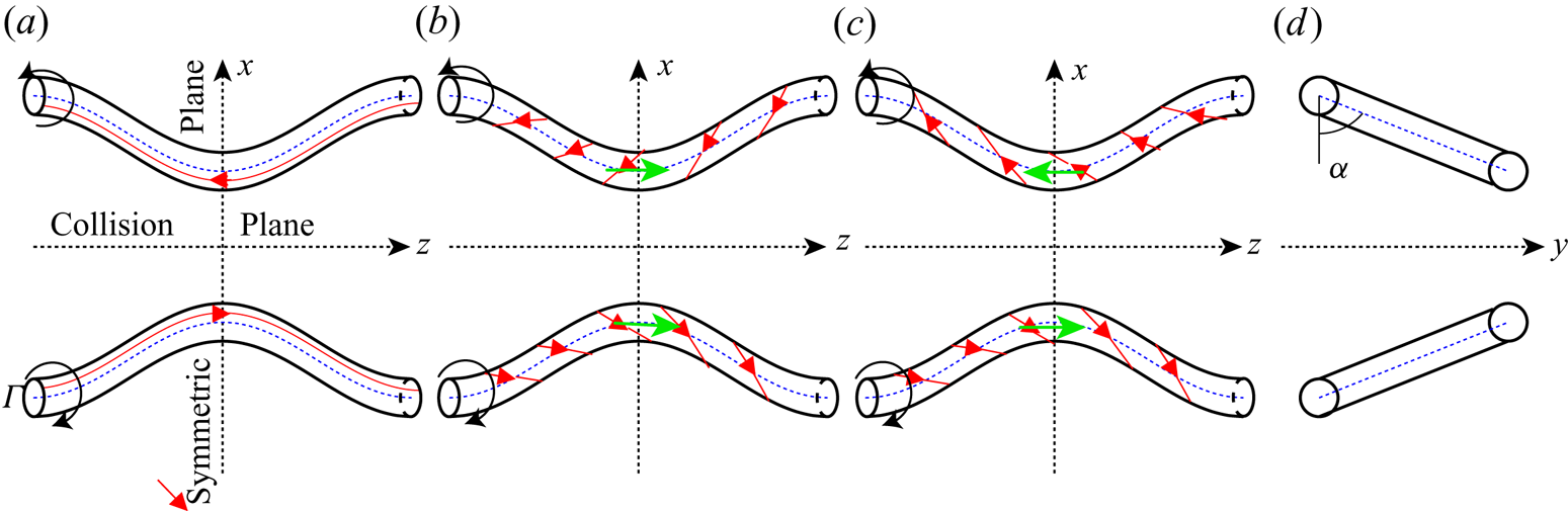
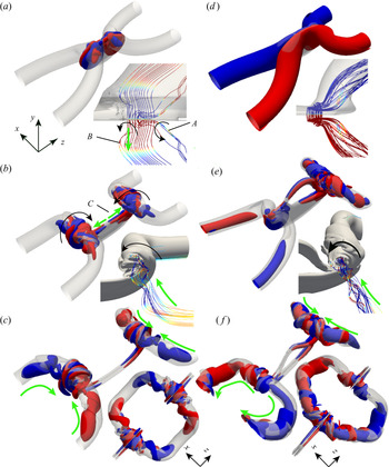
Depending on the directions of axial flows, three different initial configurations are considered (figure 1): unpolarized (no axial flow), counter-polarized (i.e. the same direction of axial flow) and co-polarized (i.e. opposite directions of axial flow). For the polarized case, we can define the initial polarization strength as  $q=u_{z,0}/u_{\theta ,0}$, where
 $u_{z,0}$ and
 $u_{\theta ,0}$ are, respectively, the peak axial and azimuthal velocities of an unperturbed tube at
 $t^{*}=0$. Note that the polarization strength
 $q$ defined here is the inverse of the swirling number typically employed for the linear instability analysis. To quantify the effect of an initial axial flow, we examine vortex tubes with several different initial strengths:
 $q=\{1/4,1/3,1/2,2/3,1,4/3\}$. For even larger
 $q$ values, the vortices become very unstable (Mayer & Powell Reference Mayer and Powell1992) and break up before reconnection – hence are not considered.
Schematic of the initial configurations: (a) unpolarized, (b) counter-polarized and (c) co-polarized cases with (d) showing the side view. The red solid lines with arrows denote the vortex lines, and the black and green arrows represent directions of vortex rotation and axial flows, respectively. The planes at  $x=0$ and
 $z=0$ denote collision
 $S_c$ and symmetric
 $S_s$ planes, respectively.

3. Results for the counter-polarized cases
We first consider the counter-polarized cases as they have zero net helicity and resemble the well-studied unpolarized cases. The co-polarized cases are discussed in the following section. Note that the results presented are primarily for  $Re=5000$. The effects of changing
 $Re$ are discussed in later sections to illustrate some specific points, but, in general, the results are qualitatively similar to those at
 $Re=5000$.
3.1. Reconnection process
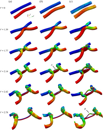
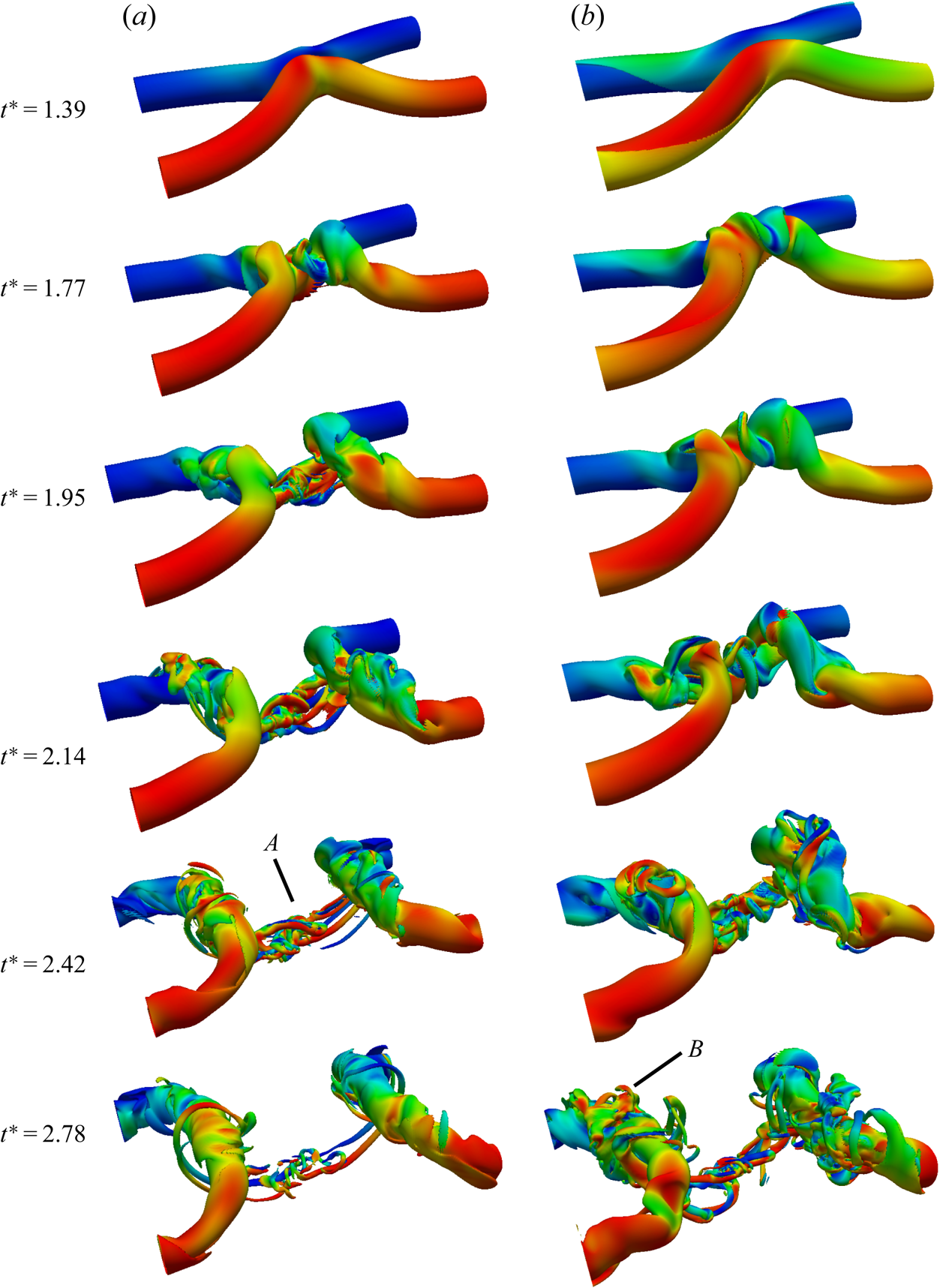
Figure 2(a–c) (and supplementary movie 1 available at https://doi.org/10.1017/jfm.2021.517) shows the time progression of the reconnection based on the vorticity magnitude isosurface  $|\boldsymbol {\omega }|=0.4\omega _0$ for
 $q=0$,
 $q=0.5$ and
 $q=1$ cases, respectively. For
 $q=0$ (i.e. the unpolarized) case, the entire evolution is similar to that described by Hussain & Duraisamy (Reference Hussain and Duraisamy2011) for
 $Re=2000$. First, the tubes approach each other due to self-induction and become flattened in the collision region. Then the viscous cross-diffusion annihilates the circulation at the contact point and this circulation transfers from the symmetry plane
 $S_s$ to the collision plane
 $S_c$. The connected vortex lines form the transverse vorticity structures (called bridges), and the remnant unreconnected parts form two parallel thin sheet-like structures (called threads), which further roll up into vortex dipoles. Due to the induced velocity of the two bridges, the curvature of the threads reverses at a late time, causing the slowdown of the reconnection. Consequently, the reconnection is not complete.
Isosurfaces of vorticity magnitude  $|\boldsymbol {\omega }|=0.4\omega _0$ shaded with contours of axial vorticity
 $\omega _z$ at
 $Re=5000$ for (a)
 $q=0$ (unpolarized case), (b) counter-polarized
 $q=0.5$ and (c) counter-polarized
 $q=1$. The solid black lines at
 $t^{*}=0$ denote the vortex lines. See also supplementary movie 1 for the full time evolution of vortical structures for all
 $q$ cases.

For the counter-polarized cases, the initial sinusoidal displacements of the vortex axis travel along the tubes in the same direction when they approach each other. For the weakly polarized case (i.e.  $q=0.5$), the flow evolution is quite similar to the unpolarized case, except for a slight difference in the thread. For example, the dipole head separates from the tail at
 $t^{*}=2.14$ (region
 $A$ in figure 2). For the strongly polarized case (i.e.
 $q=1$), the differences in the thread are more apparent and persist until the late time of reconnection (see region
 $B$ in figure 2). Due to the symmetry with respect to the collision
 $S_c$ plane, the vortex ring formed after reconnection has zero net helicity for all cases. However, due to the twist initially carried by the vortex tubes and generated during reconnection, the helicity density, even for the unpolarized case, is not everywhere zero. The distribution and evolution of helicity density are discussed in § 3.4.
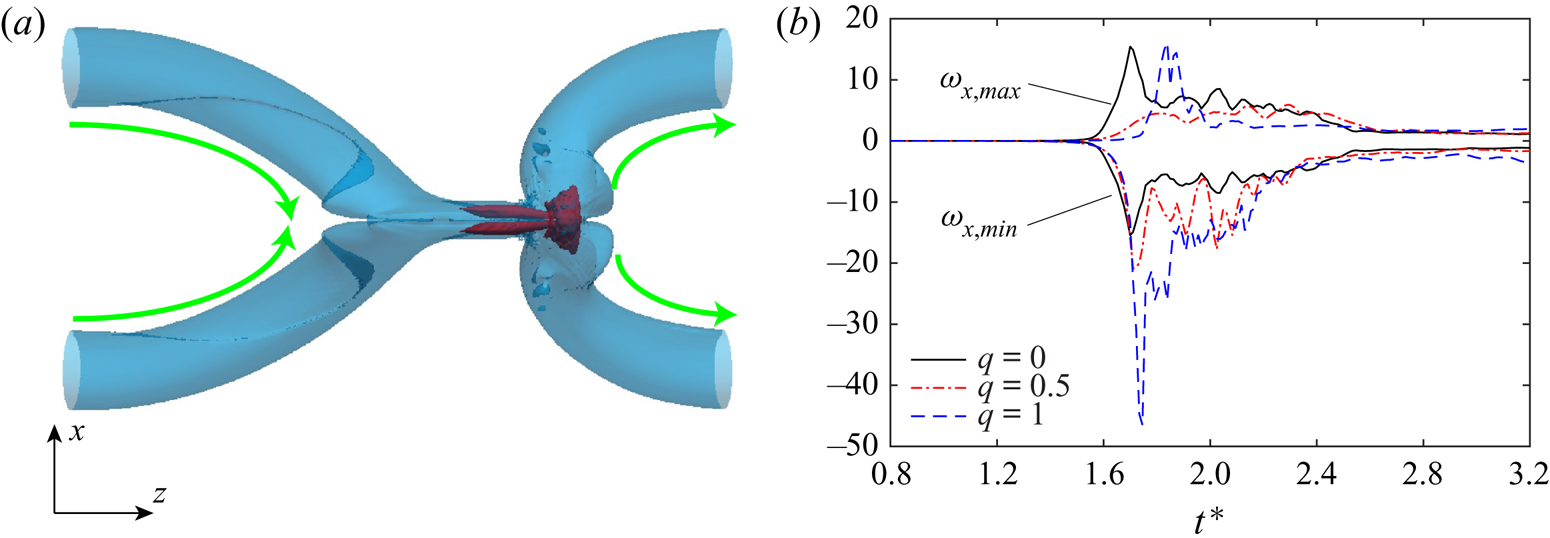
Due to the presence of initial axial flow, the symmetry about the initial symmetric plane  $S_s$ is lost for the counter-polarized cases. The left and right bridges are compressed and stretched, respectively (figure 3a); consequently, the vorticity distribution is no longer identical between the two bridges. Figure 3(b) shows the evolution of maximum vorticity in each bridge (which corresponds to the maximum and minimum of
 $\omega _x$ in the collision plane
 $S_c$) for
 $q=0$,
 $0.5$ and
 $1$ cases. Both
 $\omega _{x,min}$ and
 $\omega _{x,max}$ are initially zero before reconnection occurs and increase during reconnection, which is then followed by a decrease after reconnection. Different from the unpolarized case, where the magnitude of
 $\omega _{x,min}$ is the same as that of
 $\omega _{x,max}$, the former becomes larger in magnitude than the latter for the polarized case. In addition, the peak of
 $\omega _{x,min}$ increases with increasing
 $q$, which is due to intense vortex stretching caused by the imposed axial flow. Note that
 $\omega _{x,max}$ rapidly increases at late time (i.e.
 $t^{*}\approx 1.8$) for
 $q=1$ case, which is attributed to stretching caused by axial flow generated after reconnection (discussed later).
(a) Top view of the vortical structure at  $t^{*}=1.74$ for
 $Re=5000$ with
 $q=1$. (b) Time evolution of minimum and maximum of
 $\omega _x$ in the collision plane
 $S_c$ for different counter-polarized cases at
 $Re=5000$. Note that in (a) light (blue) and dark (red) denotes
 $|\boldsymbol {\omega }|=0.4\omega _0$ and
 $4\omega _0$, respectively, and the green arrows indicate the directions of axial flows.

3.2. Circulation transfer
As reconnection is accompanied by circulation transfer, the time variations of the circulations are generally employed to quantify the reconnection process, such as determining the reconnection rate, time, etc. As discussed above, while the symmetry about the initial symmetric plane  $S_s$ is lost for the counter-polarized cases, the symmetry regarding the collision plane
 $S_c$ is still preserved. Hence, the circulation evolution in
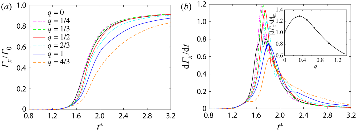
 $S_c$ can be used to measure the reconnection level, as any vortex line that passes through this plane must have been reconnected. Figure 4(a) shows the evolution of
 $\varGamma _x$ in
 $S_c$ for different
 $q$ cases at
 $Re=5000$. Consistent with previous studies (van Rees et al. Reference van Rees, Hussain and Koumoutsakos2012; McGavin & Pontin Reference McGavin and Pontin2018), the reconnection occurs later as
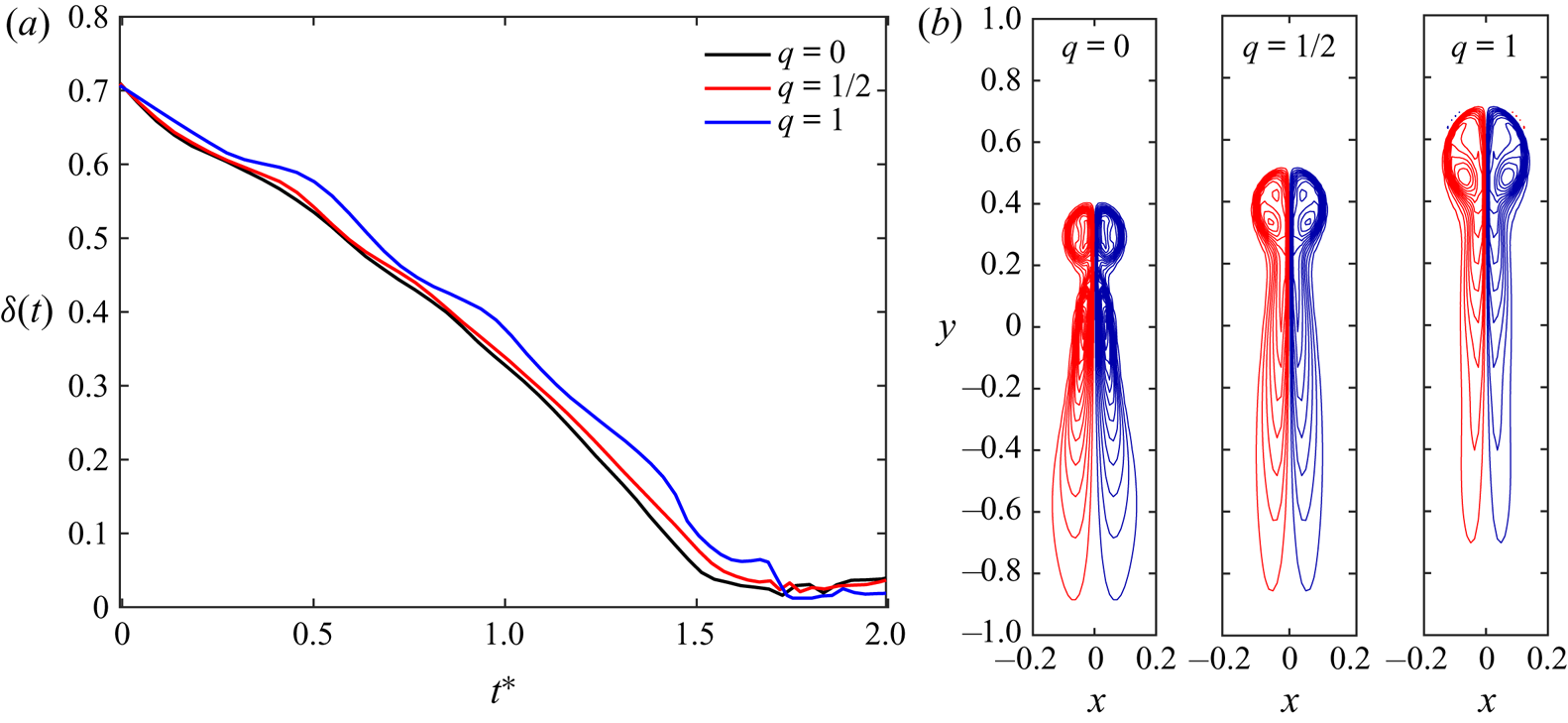
 $q$ increases, suggesting that the approach between the vortex tubes becomes slower. To confirm this, figure 5(a) shows the separation distance
 $\delta (t)$ between the two vortices before reconnection for
 $q=0$,
 $0.5$ and
 $1$ cases. Note that
 $\delta (t)$ is the distance between vorticity centroids, computed as the centroid of vorticity above 75 % of the maximum (Hussain & Duraisamy Reference Hussain and Duraisamy2011). For the unpolarized case, the minimum distance between two vortices always occurs in the
 $S_s$ plane; while for the counter-polarized case,
 $\delta (t)$ is chosen as the closest distance between vorticity centroids among all
 $x - y$ planes. Due to self-induction,
 $\delta (t)$ first decreases rapidly but then slows down when reconnection commences. With increasing
 $q$, the approach between the vortices becomes slower, which is consistent with the previous finding that the self-induced velocity of the vortex is reduced by increasing axial flows (Virk, Hussain & Kerr Reference Virk, Hussain and Kerr1995; Cheng, Lou & Lim Reference Cheng, Lou and Lim2016). Previous works on reconnection of unpolarized vortices show that the separation before reconnection scales as
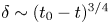 $\delta \sim (t_0 - t)^{3/4}$, where
 $t_0$ denotes the time when the centres are the closest (Hussain & Duraisamy Reference Hussain and Duraisamy2011). However, due to the oscillations, the scaling is difficult to determine for polarized cases. Recently, Yao & Hussain (Reference Yao and Hussain2020a) observed that the scaling of
 $\delta (t)$ approaches
 $\delta \sim (t_0 - t)^{1/2}$ when the core size of the tube becomes small. This
 $1/2$ scaling can be obtained through dimensional analysis based on the assumption that reconnection is a local event and the circulation is the only relevant quantity, and has been observed numerically as well as experimentally, both in quantum and classical fluids (Villois, Proment & Krstulovic Reference Villois, Proment and Krstulovic2017; Kimura & Moffatt Reference Kimura and Moffatt2018; Fonda, Sreenivasan & Lathrop Reference Fonda, Sreenivasan and Lathrop2019; Yao & Hussain Reference Yao and Hussain2020c). It would be interesting to investigate whether such
 $1/2$ scaling can be affected by the presence of axial flows. Reconnection with smaller vortex core sizes, similar to that considered in Yao & Hussain (Reference Yao and Hussain2020a), would be helpful to address this issue.
Time evolution of (a) circulation  $\varGamma _x/\varGamma _0$ and (b) circulation transfer rate
 $\partial \varGamma _x/\partial t$ for the counter-polarized cases at
 $Re=5000$. The inset in (b) shows the peak of
 $\partial \varGamma _x/\partial t$ as a function of
 $q$.

(a) Time evolution of separation distance  $\delta (t)$ for the unpolarized (
 $q=0$) and counter-polarized (
 $q=0.5$ and
 $1$) cases at
 $Re=5000$. (b) The corresponding
 $\omega _z$ distribution in the
 $x - y$ plane associated with the minimum separation at the time of the
 $\partial \varGamma _x/\partial t$ peak.

The slowdown in the approach is expected not only to cause the delay but also to reduce the speed of reconnection due to weakened compression between these two vortices – hence a decrease in circulation transfer rate  $\mathrm {d}\varGamma /\mathrm {d}t$. Figure 4(b) shows the evolution of
 $\mathrm {d}\varGamma /\mathrm {d}t$ for different
 $q$ cases. For the unpolarized (
 $q=0$) case,
 $\mathrm {d}\varGamma /\mathrm {d}t$ has dual peaks, which is consistent with the finding in Yao & Hussain (Reference Yao and Hussain2020b) for
 $Re=9000$ – showing that the reconnection process is intermittent. Consistent with the late reconnection as
 $q$ increases, the time for the peak of
 $\mathrm {d}\varGamma /\mathrm {d}t$ to occur also delays. Interestingly, the peak of
 $\mathrm {d}\varGamma /\mathrm {d}t$ non-monotonically varies with
 $q$. With increasing
 $q$, it first increases and then decreases, with the maximum occurring at
 $q =1/3$ (see the inset in figure 4b). This difference in the circulation transfer rate can be explained by examining the shape of the vortex sheet formed during reconnection. Figure 5(b) shows the vorticity distribution in the
 $x$–
 $y$ plane that produces the minimum separation at the time of peak
 $\mathrm {d}\varGamma /\mathrm {d}t$. For the unpolarized case, the heads with higher vorticity advect ahead of the tail due to mutual induction, forming a thread dipole, and then separating from the tail. In this case, as the tails have lower vorticity gradient and are more apart, most of the circulation transfer happens at the heads. No notable head–tail separation is observed for polarized cases, mainly due to the larger separation distance between the two thread vortex sheets. For the
 $q=0.5$ case, despite lower vorticity gradient, the tails also involve a significant amount of circulation transfer, presumably due to a larger contact area – resulting in a high
 $\mathrm {d}\varGamma /\mathrm {d}t$. For the
 $q=1$ case, the circulation transfer is suppressed mainly because the vortex sheets are further apart and the associated vorticity gradient is smaller.
For weakly polarized cases, although the maximum circulation transfer rate is increased, the reconnection time is shortened; hence at the end of the simulation, a similar amount of total circulation transfer to that in the unpolarized case is observed. On the other hand, for strongly polarized cases, despite the decreased circulation transfer rate, the reconnection time is increased caused by the continuous reconnection of the top thread dipole (see figure 2).
3.3. Peak vorticity and enstrophy
For vortical flows, an important quantity is enstrophy  $\varOmega =\int _V \boldsymbol {\omega }^{2}/2 \,\mathrm {d}V$, which is directly related to the generation of small scales as well as energy dissipation
 $\epsilon$ (
 $\equiv 2\nu \varOmega$ in periodic domain). The evolution equation for the enstrophy density
 $\boldsymbol {\omega }^{2}/2$ is
 \begin{equation} \frac{\mathrm{D} \boldsymbol{\omega}^{2}/2}{\mathrm{D} t}=\underbrace{\boldsymbol{\omega}\boldsymbol{\mathsf{S}}\boldsymbol{\omega}}_{production}+\underbrace{\nu \nabla^{2}(\boldsymbol{\omega}^{2}/2)}_{diffusion}-\underbrace{\nu(\boldsymbol{\nabla} \boldsymbol{\omega})^{2}}_{dissipation}, \end{equation}
where  $\mathrm {D}/\mathrm {D}t$ denotes the substantial derivative and
 $\boldsymbol{\mathsf{S}}=(\boldsymbol {\nabla } \boldsymbol {u}+ \boldsymbol {\nabla }\boldsymbol {u}^{T})/2$ is the rate of strain tensor. The terms on the right-hand side of (3.1) are enstrophy production
 $\varOmega _p$, diffusion
 $\varOmega _d$ and dissipation
 $\varOmega _\epsilon$, respectively. Note that when integrated over the whole computational domain, the enstrophy diffusion term is zero; and
 $\varOmega$ can grow due to vortex stretching and decrease due to either vortex compression or viscous dissipation.
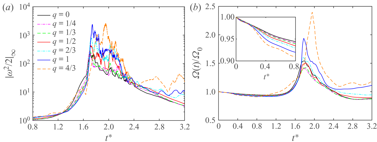
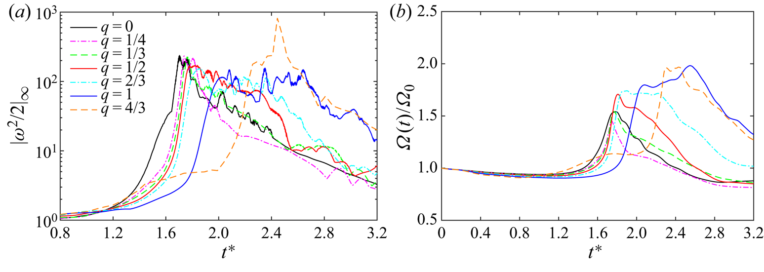
Figure 6(a) shows the time evolution of the maximum enstrophy density  $|\boldsymbol {\omega }^{2}/2|_{\infty }$. There is a transition around
 $t^{*}=1.6$: before that time,
 $|\boldsymbol {\omega }^{2}/2|_{\infty }$ is located in the initial tubes (
 $x - y$ plane), and after that it is located in the bridges. Compared with the unpolarized case, we observe a rapid increase of
 $|\boldsymbol {\omega }^{2}/2|_{\infty }$ during the reconnection for strongly polarized cases, mainly caused by the enhanced vortex stretching in the right bridge due to the opposite axial flows (see figure 3a). In addition, being a pointwise quantity,
 $|\boldsymbol {\omega }^{2}/2|_{\infty }$ experiences strong oscillations during reconnection (around
 $t^{*}=1.6$–
 $2.5$); and the oscillation slightly increases with increasing
 $q$. For the two highest
 $q$ cases, the oscillations persist until the end of the simulation.
Time evolution of (a) maximum enstrophy density  $|\boldsymbol {\omega }^{2}/2|_{\infty }$ and (b) volume-averaged enstrophy
 $\varOmega (t)$ for different
 $q$ at
 $Re=5000$.

The time evolution of enstrophy  $\varOmega$ for different
 $q$ cases is shown in figure 6(b). Due to viscous dissipation
 $\varOmega _\epsilon$,
 $\varOmega$ slowly decreases at the initial stage. The rate of decrease increases with
 $q$ (inset in figure 6b). Recently, Yao, Yang & Hussain (Reference Yao, Yang and Hussain2021) showed that for a rectilinear Batchelor vortex column, the relative decay rate of enstrophy
 $(1/\varOmega )\partial \varOmega /\partial t$ varies from
 $-2\nu /\sigma ^{2}$ to
 $-4\nu /\sigma ^{2}$ when
 $q$ increases from
 $0$ to
 $\infty$ (here,
 $\sigma$ is the vortex core size). The rapid decay of enstrophy for strongly polarized cases is consistent with the claim that helicity may inhibit energy transfer due to the role of helicity in depleting nonlinear interaction (Wu et al. Reference Wu, Ma and Zhou2007; Moffatt Reference Moffatt2014). In particular, flow becomes more Beltrami-like (
 $\boldsymbol {u}||\boldsymbol {\omega }$) as
 $q$ increases. As the tubes come close to each other and the reconnection starts,
 $\varOmega$ experiences rapid growth, due to the generation of small-scale structures (i.e. thin thread vortex sheets) through collision and stretching. After the reconnection, vortex stretching is reduced, and
 $\varOmega$ drops again due to viscous dissipation. As expected, for weakly polarized cases (typically
 $q\leqslant 0.5$), the behaviour of
 $\varOmega$ is quite similar to the unpolarized case, but the values of
 $\varOmega$ are slightly smaller for all the time. However, for large
 $q$ cases,
 $\varOmega$ becomes slightly larger than the unpolarized case, which is partially due to the excitation of the transient growth or normal-mode instability. For example, similar to that observed for the evolution of a single Batchelor vortex column with strong axial flows (Duraisamy & Lele Reference Duraisamy and Lele2008; Pradeep & Hussain Reference Pradeep and Hussain2010), large-scale helical structures develop along the vortex tubes and evolve into thin vortex layers at late times (see e.g.
 $q=4/3$ case in supplementary movie 2).
The peak of enstrophy density  $|\boldsymbol {\omega }^{2}/2|_{\infty }$ continuously increases with
 $q$. In particular,
 $|\boldsymbol {\omega }^{2}/2|_{\infty }$ triples as
 $q$ increases from
 $0$ to
 $1$. Different from
 $|\boldsymbol {\omega }^{2}/2|_{\infty }$, the peak of enstrophy
 $\varOmega _\infty$ first decreases and then increases as
 $q$ increases. The peak enstrophy becomes 1.5 times that of the unpolarized case for
 $q=4/3$ – the largest polarization strength we considered. The growth of vorticity and enstrophy is related to a key open mathematical question: whether solutions to the three-dimensional incompressible N–S equations with a smooth initial condition can develop a singularity in finite time (Doering Reference Doering2009; Moffatt & Kimura Reference Moffatt and Kimura2019a; Kang, Yun & Protas Reference Kang, Yun and Protas2020). Interaction of anti-parallel unpolarized vortex tubes has been previously employed to provide insights into this challenging problem (Kerr Reference Kerr1993; Hou & Li Reference Hou and Li2006). Although there are still no firm conclusions, most studies suggest that a finite-time singularity is unlikely to form for such configuration (Hou & Li Reference Hou and Li2008; Moffatt & Kimura Reference Moffatt and Kimura2019b; Kang et al. Reference Kang, Yun and Protas2020; Yao & Hussain Reference Yao and Hussain2020a). The observation here that reconnection of polarized vortices could yield a more rapid growth of the peak vorticity and enstrophy is somehow encouraging. It suggests that the interaction of polarized vortices might be a potential candidate for the formation of a finite-time singularity – a topic deserving further exploration.
3.4. Helicity dynamics
Another important aspect of polarized vortex dynamics is the helicity  $H$. The governing equation for the helicity density
 $h=\boldsymbol {u}\boldsymbol {\cdot }\boldsymbol {\omega }$ is
 \begin{equation} \frac{\mathrm{D} h}{\mathrm{D}t}=\underbrace{-\boldsymbol{\omega}\boldsymbol{\cdot}\boldsymbol{\nabla}(p/\rho- \boldsymbol{u}^{2}/2)}_{production}+\underbrace{\nu\nabla^{2}h}_{diffusion}-\underbrace{2\nu(\boldsymbol{\nabla} \boldsymbol{u}\boldsymbol{:} \boldsymbol{\nabla} \boldsymbol{\omega}^{T})}_{dissipation}, \end{equation}
where the terms on the right-hand side are the helicity production  $H_p$, diffusion
 $H_d$ and dissipation
 $H_\epsilon$, respectively (Kerr Reference Kerr2018a). The dissipation term can also be expressed as
 $H_d=-2\nu \boldsymbol {\omega } \boldsymbol {\cdot }(\boldsymbol {\nabla } \times \boldsymbol {\omega })$, where
 $\boldsymbol {\omega } \boldsymbol {\cdot }(\boldsymbol {\nabla } \times \boldsymbol {\omega })$ is the so-called ‘superhelicity’ (Hide Reference Hide1989; Scheeler et al. Reference Scheeler, Kleckner, Proment, Kindlmann and Irvine2014). Again, the diffusion term vanishes when integrated over the whole periodic computational domain. Different from the enstrophy production, the volume-integrated helicity production remains zero. Hence, the variation of the global helicity
 $H$ is purely due to viscous dissipation
 $H_\epsilon$. In addition, unlike the energy and enstrophy, helicity can be of either sign, and
 $H$ can grow, decrease or even change sign during the evolution – depending on the sign of
 $H_\epsilon$.
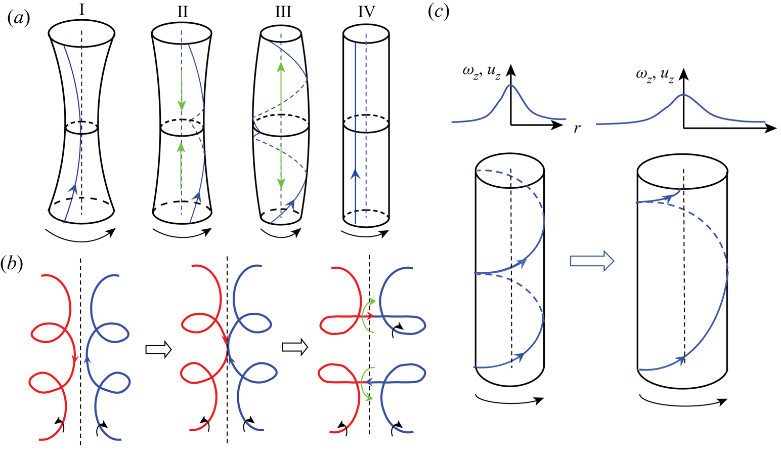
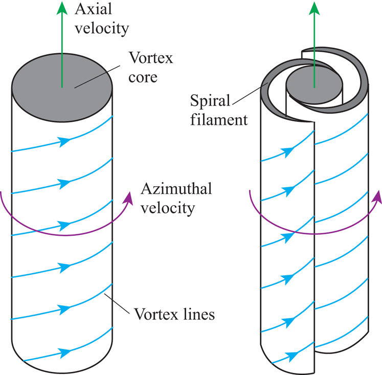
The physical mechanisms of the three terms in (3.2) are illustrated in figure 7 and explained below. For helicity production term  $H_p$, consider a vortex column that has an axial variation in core size, e.g. the vortex core is smaller in the middle than at the two ends (I in figure 7a). As the vorticity magnitude is higher in the region with small core size, the vortex lines, initially parallel to the vortex, become coiled (II in figure 7a). Note that the vortex lines are oppositely coiled with respect to the middle plane; hence positive and negative helicity densities are generated on the top and bottom parts of the vortex, respectively. The twist generated at the middle plane slowly propagates both upward and downward. This inviscid splitting mechanism serves as an important mechanism for helicity density generation. In addition, the non-uniformity of the cross-section causes variations of the pressure along with the vortex. In particular, the pressure is smaller in the middle – generating axial flows towards the centre. Due to the compression of the axial flow and the radially induced velocity of coiled vortex lines, the core size increases at the middle, and decreases at the top and bottom ends. Then the vortex lines start to untwist due to the slowdown of rotation at the middle, and the axial flows reverse direction, namely becoming towards the two ends (III in figure 7a). Due to the stretching by axial flows, the core size at the middle becomes smaller again. This process (I–III) will repeat forever in inviscid flows and will eventually arrest in viscous flows due to damping (IV in figure 7a). Hence, this mechanism also serves as a vorticity smoothing mechanism that reduces the axial variation of the vorticity magnitude (Melander & Hussain Reference Melander and Hussain1994). Similar to the enstrophy production
 $\varOmega _p$ term in the enstrophy equation, which is the main cause for energy and enstrophy cascade, the helicity production
 $H_p$ is the main mechanism for helicity cascade. Recently, Yan et al. (Reference Yan, Li, Yu, Wang and Chen2020b) further separated this production mechanism into two subprocesses, i.e. untwist and vortex stretching. Note that although the global helicity remains zero during this process, the net absolute helicity, defined as
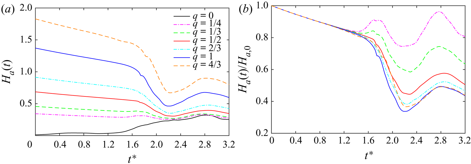
 $H_a=\int _V |h|\,\textrm {d}V$, oscillates as positive and negative helicity densities grow and decay – exactly like that observed for the evolution of the absolute helicity after reconnection (figure 8b).
Schematic of the mechanism for helicity density evolution: (a) production, (b) viscous diffusion and (c) viscous dissipation. Black arrows denote the vorticity direction, and green arrows indicate axial flow. I–IV in (a) denote the subsequent stages of helicity production.

Time evolution of (a) net absolute helicity  $H_a(t)$ and (b) normalized net absolute helicity
 $H_a(t)/H_{a,0}$ for different
 $q$ at
 $Re=5000$.

For the viscous diffusion  $H_d$, let us consider two vortex lines that are coiled in opposite directions (figure 7b). Due to self-induction, they approach each other and then reconnect. During this process, the helicity densities, which are of opposite signs in these two vortex lines, cancel each other – akin to that of enstrophy diffusion. It is clear that this process also does not alter global helicity. Finally, a vortex column with the axial flow (i.e. Batchelor vortex) can be employed to explain the viscous dissipation. Mathematically,
 $H$, which is purely in the form of twist, decreases as
 $\boldsymbol {\nabla } \boldsymbol {u}$ and
 $\boldsymbol {\nabla } \boldsymbol {\omega }$ are almost parallel to each other. Physically, when the vortex diffuses, the strengths of both vorticity and axial flow decrease. The initially coiled vortex lines become straighter, and the global helicity decreases. Scheeler et al. (Reference Scheeler, Kleckner, Proment, Kindlmann and Irvine2014) demonstrated that for the Batchelor vortex, the relative dissipation rate of helicity only depends on the viscosity and vortex core size
 $(1/H)\partial H/\partial t=-2\nu /\sigma ^{2}$.
For counter-polarized cases, due to symmetry with respect to the collision plane, the global helicity  $H$ remains zero all the time. Here, we examine the evolution of net absolute helicity
 $H_a$ (figure 8a). For the unpolarized case,
 $H_a$ is initially zero and grows slowly before reconnection, while, for the polarized case, it slowly decreases with the rate of decrease increasing with
 $q$. As explained above, the decrease is purely due to viscous dissipation – an untwisting process that occurs in vortices with axial flow. Figure 8(b) shows
 $H_a(t)$ normalized by the initial value
 $H_{a,0}$. It is clear that all curves collapse initially for different
 $q$ cases, as the decay rate of the normalized twist purely does not depend on the strength of
 $q$ (Scheeler et al. Reference Scheeler, Kleckner, Proment, Kindlmann and Irvine2014).
When the reconnection starts,  $H_a$ behaves differently for different
 $q$ cases. For the unpolarized case,
 $H_a$ increases due to the generation of the opposite-signed helicity density
 $h$ through the helicity splitting mechanism discussed above. To illustrate this, figure 9(a–c) shows the isosurfaces of
 $h$ at three different instants. Although the initial vortex tubes are unpolarized, helicity density with both positive and negative signs are generated, and its distribution is anti-symmetric with respect to
 $S_c$ and
 $S_s$ planes. At the beginning of reconnection,
 $h$ is mainly localized near the contact region. To explain the generation of the helicity density, the inset in figure 9(a) further shows the vortex lines shaded with
 $h$ around the right bridge region. The newly reconnected vortex lines, which form a cusp at the tip (see point
 $A$ in figure 9a), advect upward due to induced flow of the initial vortex tubes, while simultaneously their self-induction makes them also move up and recede away from the interaction region. During this process, the curvature of the tip decreases due to vortex stretching. The continual stretching straightens out the kinks of the vortex lines as they wrap around the unreconnected vortices at the two ends, while they also swirl around the bridges in the middle. The intense vorticity of the wrapped and stretched vortex filaments induces an axial flow within the bridges away from initial collision plane, which results in the positive
 $h$ in region
 $B$ in figure 9(a). In addition, due to the stretching by the two bridges, the threads’ cross-sections decrease, and the bridges induce axial flows along the threads (see point
 $C$ in figure 9b). Due to the presence of the axial flows, the threads also become polarized – an important reason why the threads can survive for a very long time.
Isosurfaces of normalized helicity density  $h/(u_0\omega _0)=0.5$ for
 $q=0$ (a–c) and
 $q=1$ (d–f) at (a,d)
 $t^{*}=1.77$, (b,e)
 $t^{*}=2.23$ and (c,f)
 $t^{*}=2.76$. Red and blue colours denote positive and negative
 $h$, respectively; and transparent (grey) isosurface represents
 $|\boldsymbol {\omega }|=0.4\omega _0$. The insets in (a,b) and (d,e) show the vortex lines coloured by helicity density values, with the black and green arrows denoting the direction of the vortex rotation and the axial flows, respectively. The right-bottom images in (c,f) display the top views of the structures, which are shifted in the
 $z$ direction to show the entire vortex rings.

When the bridges recede sufficiently far away from each other, the reconnection slows down, and the helicity evolution is mainly governed by the evolution of the elliptic vortex ring – formed from the unreconnected, original vortices in the periodic computational box. Due to the high vorticity magnitude in the collision plane, the bridges spin faster, enhancing coiling of the vortex lines. Furthermore, the pressure in the bridges, being lower than elsewhere in the elliptical ring, generates axial flows towards the collision plane. Following the production mechanism discussed above, the coiled vortex lines (hence  $h$) propagate away from the reconnected region as a result of core dynamics (Melander & Hussain Reference Melander and Hussain1994). From figure 9(c) (i.e. at
 $t^{*}=2.76$), the helicity density spreads over most of the newly formed vortex ring – coinciding with the occurrence of a peak of absolute helicity
 $H_a$ in figure 8(a). Due to the combined effects of viscous diffusion and collision of the axial flow, the vorticity magnitude in the collision plane continuously decreases (see figure 3b). As a result, the helicity production is suppressed due to the decrease of the pressure gradient along the vortex ring. Hence,
 $H_a$ decreases at late times due to viscous dissipation.
Absolute helicity  $H_a$ rapidly decreases when reconnection starts for the strongly polarized cases, which is mainly due to the cancellation of oppositely coiled vortex lines through viscous diffusion (figure 7b). Then,
 $H_a$ increases again due to the helicity production mechanism similar to that observed for the unpolarized case. Figure 9(d–f) shows the isosurfaces of
 $h$ at three different instants for
 $q=1$ case. One feature that distinctly differs from the unpolarized case is that the newly formed bridges are asymmetric with respect to the
 $S_s$ plane. As shown in figure 3(b), the left bridge, which is under compression, has much lower vorticity, while the right one has much higher vorticity. This difference in vorticity magnitude results in a pressure difference in these two bridges, which drives a strong axial flow within the ring from the left to the right parts (figure 9e). Note that this strong axial flow, which is opposite to that of the initial axial flow, causes the helicity density in the vortex tubes to switch sign – another important reason for the rapid decreases of the net absolute helicity. The minimum of
 $H_a$ for the
 $q=1$ case is only about 30 % of the initial value. Under the newly generated axial flows, the left bridge instead of being compressed now becomes stretched, which is consistent with the rapid increases of
 $\omega _x$ observed in figure 3(b). At late times, the newly generated axial flow even overtakes the initial axial flow, causing the absolute helicity
 $H_a$ to increase again. At
 $t^{*}=2.76$ (the time around the peak of the maximum
 $H_a$), the vortex ring fills up with
 $h$ that has different signs from the initial vortex tubes. In addition, a variation of the core size is observed around the ring. For weakly polarized cases (e.g.
 $q=1/4$), due to the combination of helicity production and diffusion,
 $H_a$ first increases then decreases. Interestingly, for all
 $q$ cases,
 $H_a$ experiences oscillations that have the same period and phase (figure 8b), caused by helicity density generation and annihilation for the newly formed elliptical vortex ring following the splitting mechanism discussed in figure 7(a).
4. Results for the co-polarized cases
We now consider the co-polarized cases, where the net helicity is non-zero. It is interesting to compare with the counter-polarized cases to see how the presence of helicity would affect the reconnection dynamics.
4.1. Reconnection process
The time evolutions of vorticity isosurfaces for the co-polarized  $q=0.5$ and
 $1$ cases are shown in figure 10(a,b) (and supplementary movie 2). The overall reconnection process is quite similar to those of unpolarized and counter-polarized cases: the vortex tubes approach each other due to self-induction and then reconnect to form bridges leaving some remnants as threads. However, due to the opposite direction of the axial flows, the symmetries regarding both
 $S_c$ and
 $S_s$ are lost; instead, it becomes diagonally symmetric, e.g.
 $\omega _x(x,y,z)=\omega _x(-x,y,-z)$. As a result, the reconnection details are quite different. Similar to the observation by McGavin & Pontin (Reference McGavin and Pontin2019), the vortex tubes approach each other in a skewed pattern, as the initial displacements travel along the tubes in opposite directions. As a consequence, the vortex sheets formed during reconnection now deform in a fully three-dimensional manner. In particular, different from the unpolarized or counter-polarized cases, where the vortex sheets roll up symmetrically to form thread dipoles, the vortex sheets here begin to twist around each other and then break up into small-scale tangled structures (region
 $A$ in figure 10). A similar process has recently been observed for the interaction of two orthogonal vortex tubes (Ostilla-Mónico et al. Reference Ostilla-Mónico, McKeown, Brenner, Rubinstein and Pumir2021). In addition, as the strength of initial axial flow increases (i.e.
 $q=1$), we observe that the generation of small scales around the bridges is more numerous (region
 $B$ in figure 10).
Isosurfaces of vorticity magnitude  $|\boldsymbol {\omega }|=0.4\omega _0$ shaded with contours of axial vorticity
 $\omega _z$ at
 $Re=5000$ for co-polarized (a)
 $q=0.5$ and (b)
 $q=1$ cases. See also supplementary movie 2 for the full time evolution of vortical structures for all
 $q$ cases.

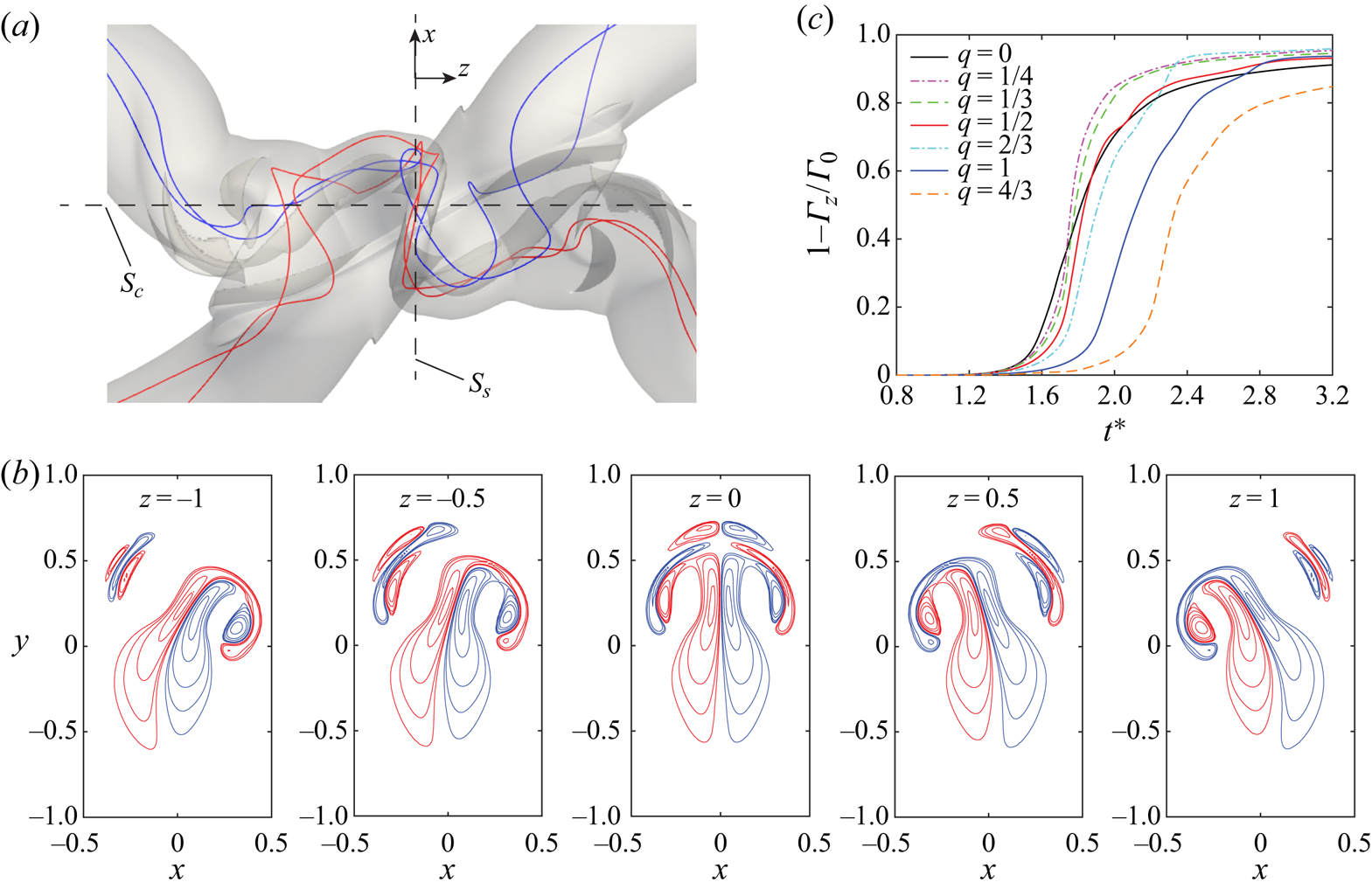
Figure 11(a) shows the top view of the vortical structure near the interaction regions along with several vortex lines at  $t^{*}=1.97$ for
 $q=1$ case. Note that different from the unpolarized or counter-polarized cases, here each vortex line can cross
 $S_s$ plane multiple times. Figure 11(b) shows the
 $\omega _z$ contours in the
 $x - y$ plane at several different
 $z$ locations. Compared with those in figure 5(b), here
 $\omega _z$ alternate signs even in one half (e.g.
 $x<0$) of the plane. Hence, in this case, reconnection can not only occur in
 $S_c$ plane but also at other places, e.g. between the dipoles in figure 11(b). However, if we assume vortex lines crossing from left to right as positive (
 $+1$) and from right to left as negative (
 $-1$), the net time each unreconnected vortex line crosses
 $S_s$ plane is always one. Hence, the circulation calculated as
 $\varGamma _z=\int _{S_c}\omega _z \,\mathrm {d}s$ can still be employed to represent the remaining circulation for unreconnected vortex lines. Figure 11(c) shows the transferred circulation (defined as
 $1-\varGamma _z/\varGamma _0$) for different
 $q$ cases. Similar to the co-polarized cases, the reconnection is delayed with increasing
 $q$. For most co-polarized cases, we observe a faster and more complete reconnection. This is again because reconnection here is fully three-dimensional and occurs in larger areas. However, for
 $q=4/3$ case, both the total circulation transfer and the transfer rate decrease, which is because the vortex tubes are more separated as the sinusoidal displacements of the vortex axis travel in opposite directions.
(a) Top view of the vortical structure at  $t^{*}=1.95$ for co-polarized
 $q=1$ case, (b) vorticity contours
 $\omega _z=[0.4\ 0.6\ 1\ 2\ 3\ 5]\omega _0$ in
 $x - y$ planes and (c) evolution of circulation transfer
 $1-\varGamma _z/\varGamma _0$ for the co-polarized cases at
 $Re=5000$. Note that in (a), the red and blues lines represent vortex lines that go through the bottom and top vortex tubes.

4.2. Peak vorticity and enstrophy
Figure 12(a) shows the time evolution of the maximum enstrophy density  $|\boldsymbol {\omega }^{2}/2|_\infty$ for the co-polarized cases. As
 $q$ increases, the growth of
 $|\boldsymbol {\omega }^{2}/2|_\infty$ is delayed, which is consistent with the late reconnection observed in figure 11(c). Unlike the counter-polarized cases, where the global peak of
 $|\boldsymbol {\omega }^{2}/2|_\infty$ rapidly increases with
 $q$, for the co-polarized cases, it slightly decreases as
 $q$ increases. This is because the strong vortex stretching experienced by the co-polarized cases due to initial axial flows softens. Interestingly, there is a sharp peak at a late time (i.e. around
 $t^{*}=2.42$) for the
 $q=4/3$ case. By examining the flow field at that instant (not shown), we find that this sharp peak is due to a strongly localized stretching.
Time evolution of (a) the maximum enstrophy density  $|\boldsymbol {\omega }^{2}/2|_\infty (t)$ and (b) the enstrophy
 $\varOmega (t)$ for co-polarized different
 $q$ at
 $Re=5000$.

Similar to the counter-polarized cases, the initial evolution of  $\varOmega$ confirms that introducing axial flows can inhibit both energy cascade and dissipation (figure 12b). Overall, the growth of the enstrophy is delayed as
 $q$ increases, which is again due to the postponing of the reconnection. One exception is for the
 $q=4/3$ case, where
 $\varOmega$ experiences a slow increase even before reconnection – presumably due to the excitation of the instability mode similar to that for an isolated unstable Batchelor vortex (Duraisamy & Lele Reference Duraisamy and Lele2008). For weakly polarized cases (i.e.
 $q<0.5$),
 $\varOmega$ is always smaller than for the unpolarized case – similar to that observed for counter-polarized cases. For strongly polarized cases,
 $\varOmega$ becomes larger after reconnection, and the peak enstrophy is roughly the same as that of the counter-polarized cases during reconnection. One feature that is different from the counter-polarized cases is that
 $\varOmega$ does not rapidly decrease after reconnection; instead, it remains at a large value for quite a long period. Again, this larger enstrophy at the late time is mainly due to the generation of small scales by the instability of the swirling vortex ring (e.g. see structures at
 $t^{*}=2.78$ in figure 10). Hence, in general, the energy cascade and dissipation are stronger for the co-polarized cases than for the counter-polarized cases.
4.3. Helicity dynamics
Figure 13(a) shows the evolution of absolute helicity  $H_a$ (normalized by its initial value
 $H_{a,0}$) for different
 $q$ cases. Consistent with counter-polarized cases,
 $H_a/H_{a,0}$ initially collapses for all cases and starts to deviate from each other as reconnection starts. In addition, as each vortex tube loses (twist) helicity at the same rate as the counter-polarized cases, the initial decay rate is the same as that shown in figure 8(b). But, the absence of helicity density cancellation in the co-polarized cases causes
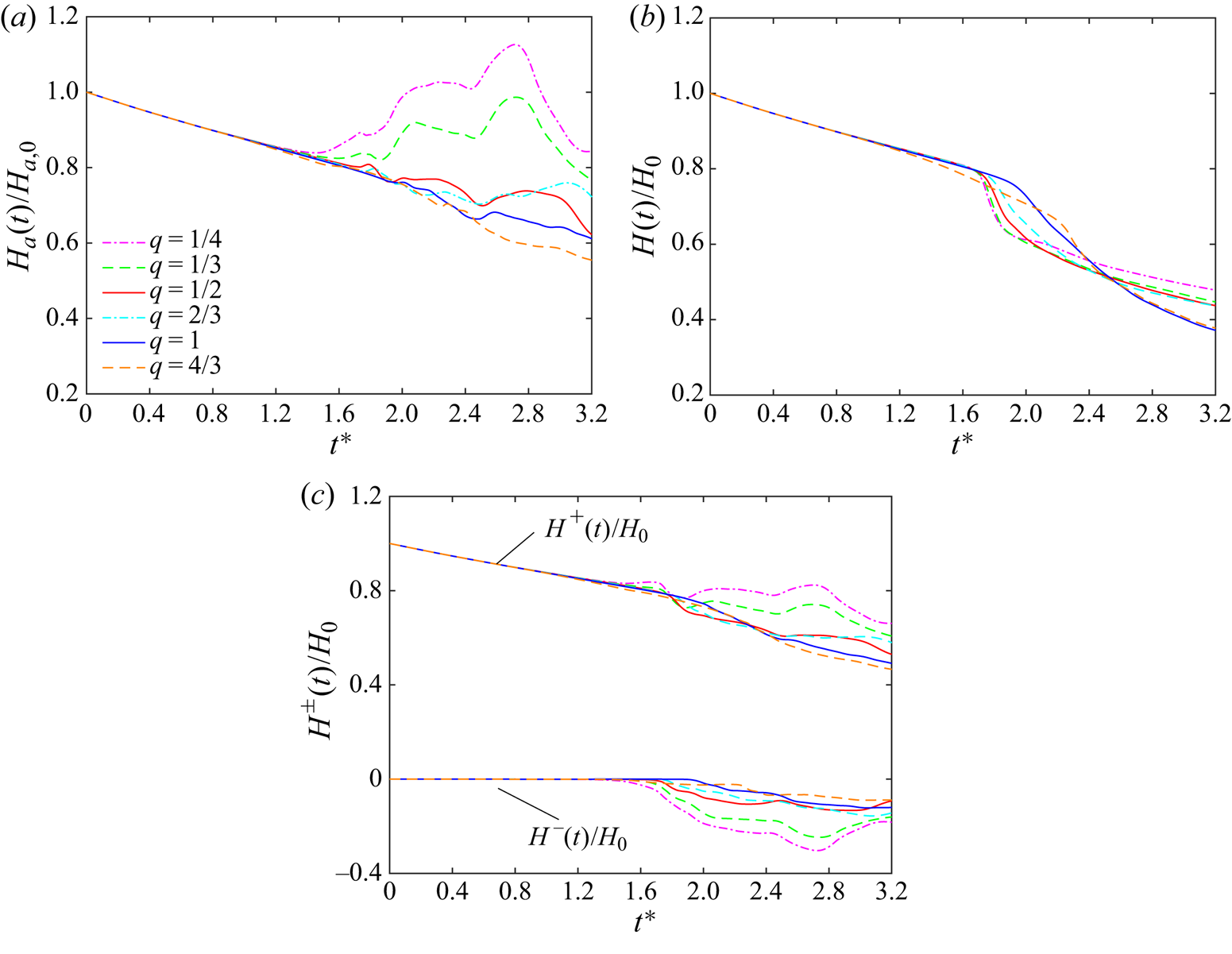
 $H_a/H_{a,0}$ to decay much slower than in the counter-polarized cases. For the weakly polarized case,
 $H_a/H_{a,0}$ even exceeds the initial value, which is due to the generation and propagation of both positive and negative helical waves during reconnection. Figure 13(b) shows the global helicity
 $H(t)$ (normalized by its initial value
 $H_{0}$), which continuously decreases due to viscous dissipation. Similar to the behaviour of energy, the decay of
 $H/H_0$ is more rapid during reconnection, suggesting that reconnection can enhance the helicity cascade and dissipation. Note that
 $H/H_0$ is much smaller than
 $H_a/H_{a,0}$ at late times, which implies that significant amounts of the oppositely polarized structures are generated during reconnection. To confirm this, figure 13(c) further shows the evolution of positive and negative helicities, calculated as
 $H^{\pm }=\int _V h^{\pm } \,\textrm {d}V$. As expected,
 $H^{-}/H_0$ remains zero for all cases before reconnection, and increases during reconnection. The relative generation of negative helicity
 $H^{-}/H_0$ decreases with
 $q$. Correspondingly, the associated positive helicity generation is also suppressed as
 $q$ increases.
Time evolution of (a) total helicity  $H$, (b) absolute helicity
 $H_a$ and (c) positive and negative helicity
 $H^{\pm }$ (normalized by their initial values) for different
 $q$ at
 $Re=5000$.

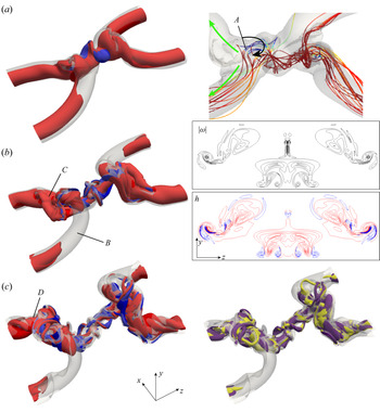
To better illustrate the generation of negative helical structures, figure 14 shows the isosurfaces of helicity density  $h$ at three different instants for
 $q=1$ case. It is clear that although the structures are predominately positively polarized, structures with negative
 $h$ develop as reconnection starts and are mainly located in the contact region. When the vortex tubes approach each other, part of the vortex tube is pulled to the top of the other tube. During this process, the associated initially coiled vortex lines are first uncoiled and then become oppositely coiled (see region
 $A$ in figure 14a). They form hairpin-like negatively polarized structures, whose induced motion, in turn, suppresses the axial flows in one tube but enhances them in the other. As a result, the newly generated swirling ring becomes partially polarized: almost unpolarized at the upstream side (region
 $B$ in figure 14b) and strongly polarized at the downstream side (region
 $C$ in figure 14b). From the vorticity and helicity iso-contours in the
 $S_c$ plane, it is clear that strong vortical regions are associated with large values of helicity density. In addition, structures with negative
 $h$ are mostly tube-like. The increased axial flow downstream augments the instability (presumably azimuthal
 $m=2$ mode; region
 $D$ in figure 14c), which then causes the vortex ring to break up and generate numerous small-scale polarized structures with negative
 $h$ structures mostly embedded within positive ones. This indicates that, along with the energy cascade, there is also a notable helicity cascade, which would then be dissipated by viscosity. This finding physically confirms the recent claim by Kessar et al. (Reference Kessar, Plunian, Stepanov and Balarac2015) that, for the forward energy cascade, it is essential for flows having strong positive
 $h$ to generate negative
 $h$. Otherwise, based on the study of Biferale, Musacchio & Toschi (Reference Biferale, Musacchio and Toschi2012) by solving the so-called decimated N–S equation (keeping only positive or negative helical modes), the energy cascade would become inverse.
Isosurfaces of normalized helicity density  $h/(u_0\omega _0)=0.5$ for
 $q=1$ at (a)
 $t^{*}=1.97$, (b)
 $t^{*}=2.19$ and (c)
 $t^{*}=2.51$. Red and blue colours denote positive and negative
 $h$, respectively; and transparent (grey) isosurface represents
 $|\boldsymbol {\omega }|=0.4\omega _0$. The right-hand panel of (a) shows the vortex lines coloured by helicity density around the interaction region, that of (b) shows the vorticity and helicity isocontours in
 $S_c$ plane and that of (c) shows the helicity dissipation with yellow and purple colours denoting positive and negative values, respectively.

5. Discussion
5.1. Reynolds number effect
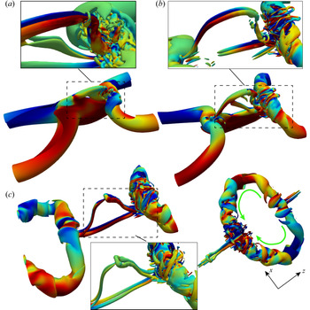
A recent study of reconnection of unpolarized vortices at higher Reynolds number demonstrated that the threads, which form head–tail structures, develop into a series of thread dipoles, and some of these dipoles undergo a second generation of reconnection forming finer structures, such as vortex rings and hairpin packets (Yao & Hussain Reference Yao and Hussain2020b). Hence, it would be worthwhile to examine the reconnections of polarized vortices at higher Reynolds numbers. Figure 15 (and supplementary movie 3) shows the evolution of vortical structures based on the vorticity magnitude isosurface for the counter-polarized  $q=1$ case at
 $Re=9000$. In the interaction region, having strong shear, the
 $\lambda _2$ criterion (Jeong & Hussain Reference Jeong and Hussain1995) is also employed to better visualize the tube-like structures. The flow evolution is quite similar to that at
 $Re=5000$ (figure 2), especially in the bridges. However, the very thin vortex sheet, formed from two vortex tubes colliding, rolls up into multiple pairs of vortex dipoles (inset in figure 15a). Then, the top vortex dipole undergoes a further reconnection, which is further clear evidence for the reconnection cascade scenario initially proposed by Melander & Hussain (Reference Melander and Hussain1988). The second reconnection follows the same manner as the first reconnection, with one bridge being stronger than the other. Secondary reconnections repeatedly occur for the top thread dipole (e.g. see figure 15c). Besides, the core of the vortex ring is strongly distorted, and the variation of the core size becomes more distinct, where the bridge under compression has a much larger core size than the one that under stretching.
Vorticity magnitude isosurfaces at  $40\,\%$ of
 $\omega _0$ shaded with levels of axial vorticity
 $\omega _z$ at
 $Re=9000$ for counter-polarized
 $q=1$ case at (a)
 $t^{*}=1.81$, (b)
 $t^{*}=2.21$ and (c)
 $t^{*}=2.74$. The inset in each panel shows the
 $\lambda _2$ structures (shaded with helicity density) in the reconnection region. Note that the right-hand image in (c) shows the top view of
 $\lambda _2$ structure, which is shifted in the
 $z$ direction to show the entire vortex ring with the green arrow denoting the directions of axial flows. See also supplementary movie 3 for the full time evolution of vortical structures.

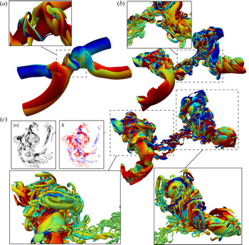
The evolution of vortical structures for the co-polarized  $q=1$ case at
 $Re=9000$ is displayed in figure 16 (and supplementary movie 4). The early stages at
 $Re = 9000$ are similar to those observed at
 $Re = 5000$: the vortex tubes collide in a skewed pattern. By comparing between the co- and counter-polarized (or unpolarized) cases, it is clear that at this high
 $Re$, the reconnection dynamics is significantly altered by the presence of net global helicity. Although multiple dipoles are formed in the threads (inset in figure 16a), they are now cross-linked, which then interact with each other in a very complex manner. Hence, a clear reconnection cascade of threads, like that for the counter-polarized case, is not observed for this case. In addition, the threads, which have opposite axial flows, break up into numerous small scales (inset in figure 16b). Note that more fine structures are developed at this
 $Re$ compared to that at
 $Re = 5000$. Due to lower viscosity, the smaller scales can survive longer, and further interact, reconnect and break up into even smaller filaments – forming a turbulent cloud comprised of tangles of slender vortices. In addition, compared to that at
 $Re=5000$, the newly formed vortex ring becomes more unstable, and the vortex core of the bridges breaks up with numerous, finer hairpin vortical structures wrapping around them – akin to that observed in vortex–turbulent interaction (Pradeep & Hussain Reference Pradeep and Hussain2010). This is also consistent with the finding of Duraisamy & Lele (Reference Duraisamy and Lele2008) that the excitation of normal-mode instability for a Batchelor vortex generates numerous helical structures.
Vorticity magnitude isosurfaces at  $40\,\%$ of
 $\omega _0$ shaded with contours of axial vorticity
 $\omega _z$ at
 $Re=9000$ for co-polarized
 $q=1$ case at (a)
 $t^{*}=1.97$, (b)
 $t^{*}=2.50$ and (c)
 $t^{*}=2.98$. The
 $\lambda _2$ structures shaded with helicity density are shown in the insets. The left-hand panels in (c) are the vorticity and helicity density contours in
 $S_c$ plane. See also supplementary movie 4 for the full time evolution of vortical structures.

For most quantities, such as circulation transfer, enstrophy and absolute helicity, their variations with  $q$ at
 $Re=9000$ are quite similar to those at
 $Re=5000$. Here, we mainly compare enstrophy and helicity between
 $Re=5000$ and
 $9000$ for
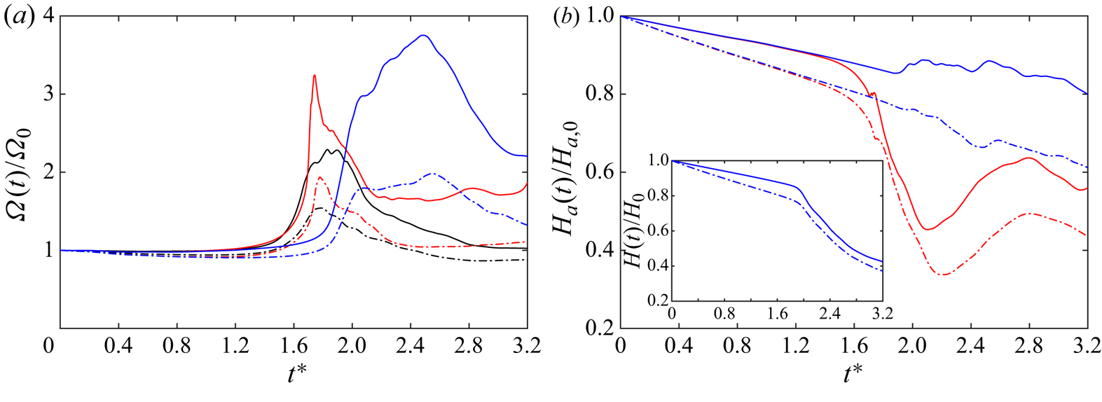
 $q=1$ cases. Figure 17(a) shows the evolution of enstrophy
 $\varOmega$ for counter- and co-polarized
 $q=1$ cases. Note that the unpolarized case is also included for comparison. As viscous dissipation is suppressed for
 $Re=9000$ cases,
 $\varOmega$ remains almost constant before reconnection. During reconnection,
 $\varOmega$ experiences rapid growth, with the peak increasing with
 $Re$. The time when the peak is reached seems to be less dependent on
 $Re$. Compared with unpolarized and co-polarized cases,
 $\varOmega$ for the co-polarized case experiences a much longer period of increase. The large peak for co-polarized
 $q=1$ case at late time (i.e.
 $t^{*}=2.5$) is consistent with the generation of numerous small-scale structures after reconnection (figure 16c).
Time evolution of (a) enstrophy  $\varOmega (t)$ and (b) net absolute helicity
 $H_a(t)$ normalized by their initial value for the unpolarized
 $q=0$ (black), counter-polarized (red) and co-polarized (blue)
 $q=1$ cases at
 $Re=5000$ (dot-dashed line) and
 $9000$ (solid line). The inset in (b) shows the total helicity
 $H(t)$ for co-polarized
 $q=1$ case at
 $Re=5000$ and
 $9000$.

Figure 17(b) shows the evolution of normalized absolute helicity  $H_a/H_{a,0}$ for the counter- and co-polarized
 $q=1$ cases. Although the vortex tubes initially have different polarization, the helicity dissipation is the same when the interaction between the two vortex tubes is weak as they are far apart. Hence, at the same
 $Re$,
 $H_a/H_{a,0}$ initially collapses between the counter- and co-polarized cases. During reconnection,
 $H_a/H_{a,0}$ rapidly decreases for counter-polarized cases due to cross-diffusion. For the co-polarized case,
 $H_a/H_{a,0}$ slightly increases during reconnection for
 $Re=9000$, which is again due to the generation of numerous polarized small scales. The inset in figure 17(b) further compares the normalized global helicity
 $H/H_0$ between
 $Re=5000$ and
 $9000$ for the co-polarized
 $q=1$ case. Here
 $H/H_0$ continuously decays for both cases, but the decay rate becomes slower for
 $Re=9000$ due to the reduced viscous effect. Note that the difference of
 $H_a/H_{a,0}$ between
 $Re=5000$ and
 $9000$ is much larger than that for
 $H/H_0$. This indicates that the generation of structures with
 ${\pm }h$ increases with increasing
 $Re$, which is speculated to be related to the more rapid generation of small-scale structures at high
 $Re$.
5.2. Energy and helicity cascade
In turbulent flows, energy is on average continuously transferred from energy-containing large scales to energy-dissipative smaller scales, which are expected to be statistically independent of the large-scale structures at high Reynolds numbers. Numerous experimental and numerical studies have shown that the slope of the energy spectrum in the inertial range follows  $-5/3$, first derived by Kolmogorov (Reference Kolmogorov1941) based on dimensional analysis. Recently, this
 $-5/3$ spectrum has also been observed for the reconnection of unpolarized vortical structures at high Reynolds numbers (van Rees et al. Reference van Rees, Hussain and Koumoutsakos2012; Yao & Hussain Reference Yao and Hussain2020b). Whether or how the energy cascade is affected by the presence of axial flows (or helicity) is as yet unclear. It has long been thought that the inviscid invariants play significant roles in determining the direction of the energy cascade (Frisch Reference Frisch1995). For example, the presence of two positive definite invariants (i.e. energy and enstrophy) for two-dimensional incompressible N–S equations does not allow a simultaneous transfer of both quantities either to small or to large scales. Hence, for two-dimensional turbulence, energy is transferred backward to larger scales while enstrophy is transferred forward to the small scales (Boffetta & Ecke Reference Boffetta and Ecke2012). Three-dimensional incompressible N–S equations also possess two inviscid invariants: energy and helicity. However, different from enstrophy, helicity is not positively defined and does not impose any constraints on the energy cascade; hence, both energy and helicity can be transferred to small scales in three-dimensional turbulent flows. Helicity cascade was first studied in Brissaud et al. (Reference Brissaud, Frisch, Léorat, Lesieur and Mazure1973), where two possibilities were considered. The first was a pure helicity cascade, where the energy and helicity spectra follow
 $E(k)\sim k^{-7/3}$ and
 $H(k)\sim k^{-4/3}$, respectively. The second one was a joint cascade, and for this case the energy and helicity spectra both follow
 $k^{-5/3}$. It was argued theoretically by Kraichnan (Reference Kraichnan1973) that the second possibility is more plausible and has been observed numerically by Borue & Orszag (Reference Borue and Orszag1997) and Chen, Chen & Eyink (Reference Chen, Chen and Eyink2003) in homogeneous isotropic turbulence (HIT) with a large-scale helical forcing.
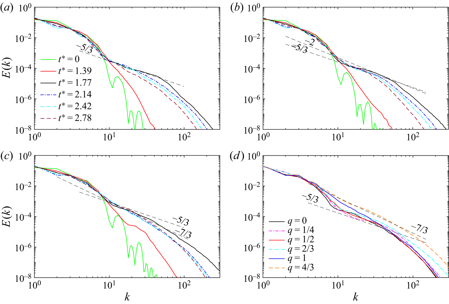
The flow structure analysis in the previous sections clearly demonstrates that energy cascade during reconnection is strongly influenced by the polarization of the vortices. To further confirm this, we present in figure 18 the evolution of energy spectra  $E(k)$ for the unpolarized (
 $q=0$) and counter-polarized (
 $q=0.5$ and
 $1$) cases at
 $Re=9000$. For
 $q=0$ case, energy is initially concentrated at small wavenumbers, and is continuously manifested at large wavenumbers as the reconnection starts. At
 $t^{*}=1.77$, the spectra develop a distinct power law with
 $-5/3$ slope. At late times, the energy at high wavenumbers gradually decays by dissipation, and the range of the power-law regimes is reduced again. The overall evolutions of
 $E(k)$ for polarized cases are quite similar to the unpolarized case. But, interestingly, the maximum slope (occurring around the time of peak enstrophy) varies with
 $q$. For example, the maximum slope falls in the range between
 $-5/3$ and
 $-2$ for
 $q=0.5$ case and becomes around
 $-7/3$ for
 $q=1$ case. Figure 18(d) further shows the spectra around the time of peak enstrophy for all
 $q$ cases. Although the global helicity
 $H$ is zero for all these cases, it is clear that polarization has a significant effect on the energy cascade. Increasing the polarization strength steepens the energy spectra, with a scaling law varying from a Kolmogorov
 $k^{-5/3}$ to a non-Kolmogorov
 $k^{-7/3}$ as
 $q$ increases from
 $0$ to
 $4/3$.
Evolution of kinetic energy spectra  $E(k)$ for counter-polarized vortex reconnection at
 $Re=9000$ with (a)
 $q=0$, (b)
 $q=0.5$ and (c)
 $q=1$ cases; and (d)
 $E(k)$ for different
 $q$ at the time of peak vorticity.

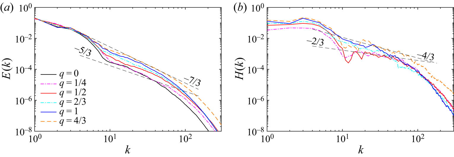
Figure 19(a) shows the energy spectra around the time of peak enstrophy for the co-polarized cases at  $Re=9000$. Interestingly, although the reconnection dynamics is significantly different, the behaviour of energy spectra is overall quite similar to that of the counter-polarized cases. Again, increasing the polarization strength steepens the energy spectra in the inertial range, with a scaling law varying from a Kolmogorov
 $k^{-5/3}$ for unpolarized
 $q=0$ to a non-Kolmogorov
 $k^{-7/3}$ for strongly polarized cases (
 $q=4/3$). As non-zero helicity is presented for the co-polarized case, figure 19(b) further shows the helicity spectra
 $H(k)$ at the same time as
 $E(k)$. As the global helicity
 $H$ increases with
 $q$, so does the magnitude of
 $H(k)$. Due to strong oscillations occurring at high wavenumbers, the slopes of
 $H(k)$ cannot be accurately determined. However, it seems that, as
 $q$ increases, the slope varies from
 $-2/3$ to
 $-4/3$ – the latter being the value suggested by Brissaud et al. (Reference Brissaud, Frisch, Léorat, Lesieur and Mazure1973) for pure helicity cascade. Such variations in energy and helicity spectra were also observed by Kessar et al. (Reference Kessar, Plunian, Stepanov and Balarac2015) for HIT with controlled helicity injection using a dynamical forcing. The occurrence of the non-Kolmogorov energy spectra through reconnection of strongly polarized vortices is rather striking. It was also observed by van Rees et al. (Reference van Rees, Hussain and Koumoutsakos2012) for a slightly higher
 $Re$ (i.e. 10 000). Further studies at even higher
 $Re$ are required to ensure that the phenomena observed here are robust and universal.
(a) Energy  $E(k)$ and (b) helicity
 $H(k)$ spectra for co-polarized vortex reconnection at
 $Re=9000$ with different
 $q$ at the time of peak vorticity. The straight dashed lines correspond to the
 $-5/3$ and
 $-7/3$ slopes in (a) and to
 $-2/3$ and
 $-4/3$ in (b).

5.3. Scale locality of energy and helicity cascade
Another important aspect of turbulent energy cascade is the locality of interactions between different scales (Taylor & Green Reference Taylor and Green1937; Domaradzki & Rogallo Reference Domaradzki and Rogallo1990). Numerous studies have suggested that a vortex of a given size is stretched primarily by the strain from structures that are three to five times larger (Leung, Swaminathan & Davidson Reference Leung, Swaminathan and Davidson2012; Doan et al. Reference Doan, Swaminathan, Davidson and Tanahashi2018). Buaria, Pumir & Bodenschatz (Reference Buaria, Pumir and Bodenschatz2020) found that when vorticity at a point is strongly amplified, the nonlinearity in its local neighbourhood would markedly counteract further amplification. Recently, Yan, Li & Yu (Reference Yan, Li and Yu2020a) showed that a structure with scale  $L$ would also largely transfer its helicity to structures with scales of around
 $0.3L$.
Having observed significant differences in energy cascade for polarized vortex reconnection, we examined the polarization effect on the scale locality in energy cascade, as well as in helicity cascade. The scale-by-scale transfer and interaction are analysed following the method proposed by Davidson, Morishita & Kaneda (Reference Davidson, Morishita and Kaneda2008). The velocity  $\boldsymbol {u}$ and vorticity
 $\boldsymbol {\omega }$ are decomposed into large and small scales such that
 $\boldsymbol {u}=\boldsymbol {u}^{L}+\boldsymbol {u}^{S}$ and
 $\boldsymbol {\omega }=\boldsymbol {\omega }^{L}+\boldsymbol {\omega }^{S}$, where the superscripts
 $L$ and
 $S$ respectively denote the larger and smaller structures compared to a selected scale. Here, the spectral space bandpass filtering procedure is employed to educe the structure of a given length scale
 $L$:
 \begin{equation} \hat{\boldsymbol{u}}^{L}(\boldsymbol{k})=\frac{\alpha}{\sqrt{L}}2\kappa^{2}\textrm{e}^{-\kappa^{2}} \hat{\boldsymbol{u}}(\boldsymbol{k}), \end{equation}
where  $\kappa =kL/2$ with
 $k=|\boldsymbol {k}|$ and
 $\alpha =\sqrt {2}$.
The energy equations for the large and small scales can be obtained by taking the dot product of velocity with the N–S equations and ensemble averaging, which yields
 $$\begin{gather} \frac{\partial}{\partial t}\langle{(\boldsymbol{u}^{L})^{2}/2}={-}F_E-\nu\rangle{(\boldsymbol{\nabla}\times \boldsymbol{u}^{L})^{2}}, \end{gather}$$
 $$\begin{gather}\frac{\partial}{\partial t}\langle{(\boldsymbol{u}^{S})^{2}/2}=F_E-\nu\rangle{(\boldsymbol{\nabla}\times \boldsymbol{u}^{S})^{2}}, \end{gather}$$
where  $F_E(r)=\langle {\boldsymbol {u}^{L}\boldsymbol {\cdot }(\boldsymbol {u}^{L}\boldsymbol {\cdot } \boldsymbol {\nabla }\boldsymbol {u}^{S})-\boldsymbol {u}^{S}\boldsymbol {\cdot }(\boldsymbol {u}^{S} \boldsymbol {\cdot }\boldsymbol {\nabla }\boldsymbol {u}^{L})}\rangle $ is the energy flux from large to small scales across the scale
 $r$. From this formalism, the transfer of energy from scale
 $L$ to
 $S$ across the scale
 $r$ can be analysed by studying the energy flux
 $F_E$.
Similarly, the helicity equations for the large and small scales are (Yan et al. Reference Yan, Li and Yu2020a)
 $$\begin{gather} \frac{\partial}{\partial t}\langle{\boldsymbol{u}^{L}\boldsymbol{\cdot}\boldsymbol{\omega}^{L} }\rangle ={-}F_H-2\nu(\boldsymbol{\nabla} \boldsymbol{u}^{L}\boldsymbol{\cdot} \boldsymbol{\nabla} \boldsymbol{\omega}^{L}), \end{gather}$$
 $$\begin{gather}\frac{\partial}{\partial t}\langle{\boldsymbol{u}^{S}\boldsymbol{\cdot}\boldsymbol{\omega}^{S} }\rangle = F_H-2\nu(\boldsymbol{\nabla} \boldsymbol{u}^{S}\boldsymbol{\cdot} \boldsymbol{\nabla} \boldsymbol{\omega}^{S}), \end{gather}$$
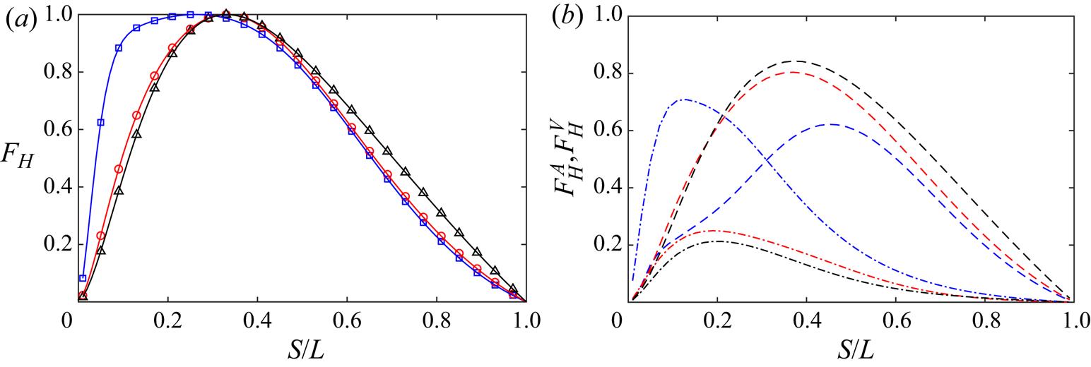
where  $F_H(r)$ is the helicity flux from large scale
 $L$ to small scale
 $S$ across the scale
 $r$, and it can be decomposed into an advection term
 $F^{A}_{H}$ and a vortex stretching term
 $F^{V}_{H}$:
 $$\begin{gather} F^{A}_H(r)=\langle{\boldsymbol{\omega}^{L}\boldsymbol{\cdot}(\boldsymbol{u} \boldsymbol{\cdot}\boldsymbol{\nabla}\boldsymbol{u}^{S})}\rangle + \langle{\boldsymbol{u}^{L}\boldsymbol{\cdot}(\boldsymbol{u}\boldsymbol{\cdot}\boldsymbol{\nabla}\boldsymbol{\omega}^{S})},\rangle \end{gather}$$
 $$\begin{gather}F^{V}_H(r)={-}\langle{\boldsymbol{u}^{L}\boldsymbol{\cdot}(\boldsymbol{\omega} \boldsymbol{\cdot}\boldsymbol{\nabla}\boldsymbol{u}^{S})}\rangle. \end{gather}$$
Recently, Yan et al. (Reference Yan, Li, Yu, Wang and Chen2020b) proposed the dual-channel helicity cascade theory, where, in addition to velocity and vorticity advection (twist or untwist), the vortex stretching is also involved in the helicity cascade process.
Following Doan et al. (Reference Doan, Swaminathan, Davidson and Tanahashi2018), we investigate the interactions between a given scale  $L$ and various smaller scales
 $S$ and thus assess the locality of the energy transfer. Three cases at
 $Re=9000$ are considered: the unpolarized (
 $q=0$) and counter- and co-polarized
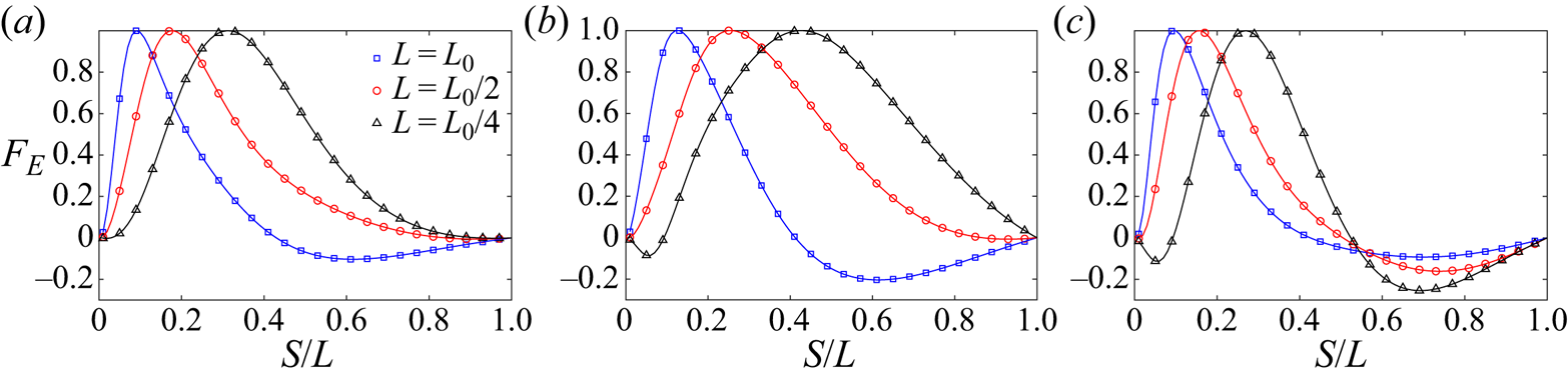
 $q=1$ cases. The normalized energy flux
 $F_E$ as a function of
 $S/L$ is shown in figure 20 for different choices of large scales
 $L=L_0$,
 $L_0/2$ and
 $L_0/4$. Here
 $L_0$ is chosen such that the bandpass filtered energy spectrum is centred around the peak of the enstrophy spectrum (i.e.
 $k_p=4$ and
 $L_0={\rm \pi} /2$). Note that positive
 $F_E$ denotes forward cascade, where the energy transfers from large scales to small scales, while negative
 $F_E$ represents inverse cascade, where the energy transfers from small scales to large scales. Let us first consider the unpolarized case. When
 $L=L_0$, energy is mostly forward transferred to small scales, peaking at
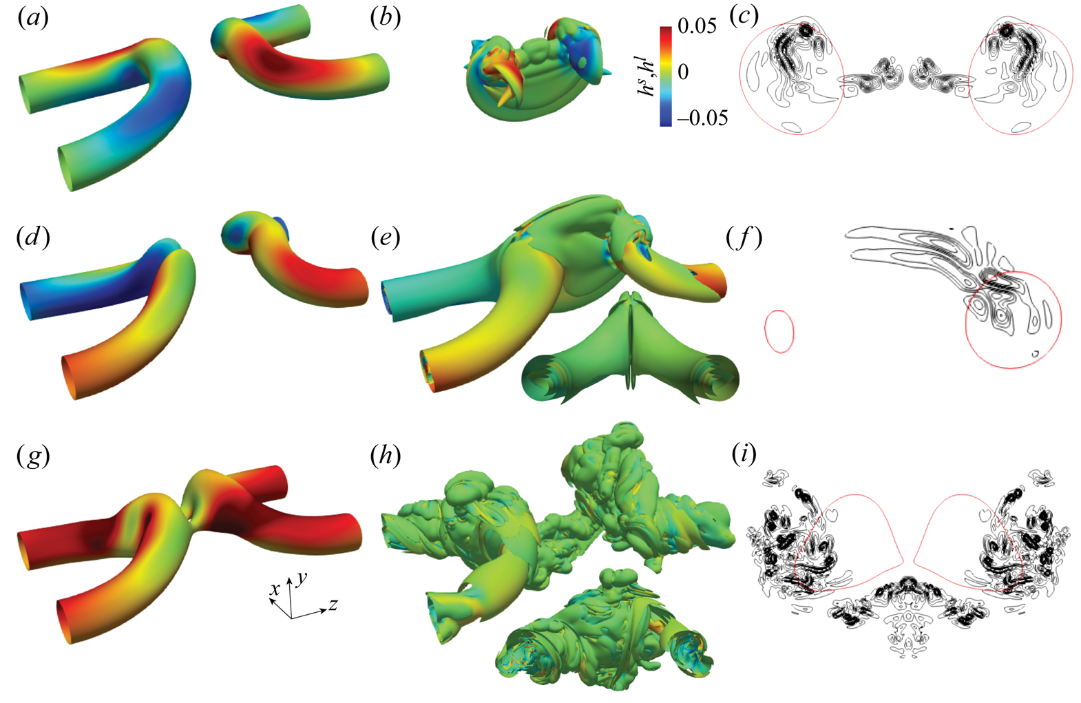
 $S/L\approx 0.1$. Figure 21(a,b) shows the vortical structures with
 $L=L_0$ and
 $S=0.1L_0$ (which corresponds to
 $k_p\approx 46$ – the upper limit of the inertial range); figure 21(c) depicts the vorticity isocontours in
 $S_c$ plane. Structures in the large-scale range mainly correspond to the reconnected main bridges, and those in the small-scale range are the stretched threads and reconnected small-scale bridgelets. This suggests that the small scales generated during reconnection are typically one order smaller than the large scales. In addition, there is also a small negative peak around
 $S/L=0.6$, implying a small portion of inverse energy transfer from the small scales. Yao & Hussain (Reference Yao and Hussain2020b) showed that this inverse cascade corresponds to the formation of bridges through the merger of small bridgelets. As the large scale
 $L$ decreases, the energy cascade becomes purely forward. In addition, the location of peak
 $F_E$ increases when
 $L$ decreases – suggesting that the scale locality becomes stronger. When the large scale is in the inertia range (i.e.
 $L=L_0/4\approx 45\eta$,
 $\eta$ being the Kolmogorov length scale), the energy is mostly transferred to
 $0.3L$, which is consistent with the finding of Doan et al. (Reference Doan, Swaminathan, Davidson and Tanahashi2018) for HIT.
Normalized energy flux  $F_E$ as a function of
 $S/L$ at the time of peak enstrophy for (a) unpolarized, (b) counter-polarized
 $q=1$ and (c) co-polarized
 $q=1$ cases at
 $Re={9000}$. Here
 $L_0$ is selected so that the bandpass filtered energy spectrum is peaked around
 $k_p=4$.

Band-filtered vortical structures in the large-scale range (a,d,g) and small-scale range (b,e,h), along with the vorticity isocontours in  $S_c$ plane (c,f,i) for (a–c)
 $q=0$, (d–f) counter-polarized
 $q=1$ and (g–i) co-polarized
 $q=1$ cases at
 $Re=9000$. Note that the large scale corresponds to structures with
 $L=L_0$ and small scales
 $S$ are those associated with peak
 $F_E$ for
 $L=L_0$. The structures are visualized based on vorticity magnitude isosurfaces (
 $|\boldsymbol {\omega }^{L}|=0.4\omega _0$ and
 $|\boldsymbol {\omega }^{S}|=0.4\omega _0$) shaded with normalized helicity density
 $h^{L}=(\boldsymbol {u}^{L}\boldsymbol {\cdot } \boldsymbol {\omega }^{L})/u_0\omega _0$ and
 $h^{S}=\boldsymbol {u}^{S}\boldsymbol {\cdot } \boldsymbol {\omega }^{S}/u_0\omega _0$ for large and small scales. The black and red contours in (c,f,i) correspond to
 $|\boldsymbol {\omega }^{S}|=[2\ 4\ 6\ 8\ 10\ 12\ 14\ 16]\omega _0$ and
 $|\boldsymbol {\omega }^{L}|=0.4\omega _0$, respectively.

For counter-polarized cases, the distribution of normalized energy flux  $F_E$ is very similar to that of the unpolarized case. The peak for the forward cascade is located at
 $S/L=0.13$,
 $0.21$ and
 $0.43$ for
 $L=L_0$,
 $L_0/2$ and
 $L_0/4$ cases, which are slightly larger than for the unpolarized case. The vortical structures with
 $L=L_0$ and
 $S=0.13L_0$ are displayed in figure 21(d–f). Again, the large scales are primarily associated with reconnected main bridges and the vortex tubes away from reconnection region. However, besides the stretched threads and reconnected small-scale bridgelets, the structures in the small-scale range also include the initial vortex tubes, which are in the form of spiral sheets. For the co-polarized case, the forward cascade is almost identical to that for the unpolarized case, but compared with the counter-polarized cases, the range of the forward cascade is much narrower. In addition, while the inverse cascade is suppressed for
 $L=L_0$, it is observed to become enhanced for
 $L=L_0/4$, peaking at
 $S/L=0.7$. This suggests that the scales of bridges are smaller than those for the unpolarized and co-polarized cases. Figure 21(g–i) reveals that the small scales also involve threads, bridges and unreconnected vortex tubes, which are again in the form of spiral sheets, but they are more irregular when compared with the counter-polarized case. In addition, the small scales are mainly clustered at the periphery of large scales.
Figure 21 clearly reveals that the physical mechanism of the energy cascade is quite different between unpolarized and polarized cases. For the unpolarized case, the small scales are mainly associated with the newly formed bridges and threads, and the energy is transferred to them through vortex stretching. However, for polarized cases, the small scales also have a significant contribution from the initial vortex tubes, which evolve into the form of spiral vortex sheets. Lundgren (Reference Lundgren1982) proposed a physical energy cascade model in the form of a spiralling vortex sheet under axial stretching. The energy, which is mainly associated with the azimuthal velocity component, can develop into a Kolmogorov  $-5/3$ spectrum. Pullin & Lundgren (Reference Pullin and Lundgren2001) further showed that including strong axial velocity in the stretched-spiral vortex model would alter the energy spectrum. Note that the dominant contribution of the energy comes from the axial velocity component in this scenario, and Pullin & Lundgren (Reference Pullin and Lundgren2001) found that the energy spectrum becomes
 $-7/3$ at large wavenumbers. The physical mechanism associated with that is sketched in figure 22, where due to the swirling and twisting effects (i.e. parts near the vortex axis rotate faster than those ways from the axis), the initially axially symmetrical vortex tubes become spiral and the energy associated with the axial velocity cascades to thin vortex sheets, which then can further break up into smaller helical vortices. The observation of spiral vortex sheets in figure 21 seems to support that the structural model proposed by Reference Pullin and LundgrenPullin & Lundgren is the main physical mechanism for the formation of the
 $k^{-7/3}$ energy spectrum observed for reconnection of strongly polarized vortices.
Schematic of the physical mechanism for energy cascade of vortex tubes with strong axial flows: vortex spiral.

To confirm this, we further examine the scale locality of helicity cascade (only for the co-polarized  $q=1$ case, as the helicity remains zero for the other two cases). Similar to the energy spectra, helicity, which is initially concentrated at small wavenumbers, transfers to large wavenumbers as the reconnection starts, and the slope of
 $H(k)$ seems to approach
 $k^{-4/3}$ in the inertial range (figure 19b). It is worth mentioning again that the
 $k^{-7/3}$ energy and
 $k^{-4/3}$ helicity spectra, which have been speculated to occur for flows with purely helical cascade, have been previously observed only for simulations of modified N–S equations with specific forcing techniques (Biferale et al. Reference Biferale, Musacchio and Toschi2012; Kessar et al. Reference Kessar, Plunian, Stepanov and Balarac2015). The occurrence of such scalings from the reconnection of two simple polarized vortices is rather encouraging, because this provides a new path to investigate helicity cascade with no need to employ truncated N–S equations. Figure 23(a) shows the normalized helicity flux
 $F_H$ as a function of
 $S/L$. Different from energy, which has both forward and inverse cascades, the helicity always forward cascades to small scales, and the ranges of forward helicity cascade are much broader when compared with energy cascades. In addition,
 $F_H$ is more self-similar than
 $F_E$, with the peak located at
 $S/L\approx 0.3$ for all the large scales
 $L$ considered. The two different contributions to the helicity cascade (5.6) at different large scales are further shown in figure 23(b). It is interesting that the advection
 $F^{A}_H$ and the vortex stretching
 $F^{V}_H$ terms behave quite differently: the contribution of
 $F^{V}_H$ to
 $F_V$ is mainly located at small scales, while
 $F^{A}_H$ dominates at relatively large scales (
 $S/L\approx 0.5$) and with a much broader range. The stronger helicity cascade due to vortex stretching at small scales is consistent with the strong forward energy cascade at these scales. For
 $L=L_0$, the contribution of
 $F^{V}_H$ is much larger than that of
 $F^{A}_H$ for
 $S/L<0.3$. For smaller
 $L$, the amplitudes of
 $F^{A}_H$ are always larger than those of
 $F^{V}_H$. This means that, at these scales, vortex stretching plays a secondary role in helicity cascade, which is consistent with the finding of Yan et al. (Reference Yan, Li and Yu2020a) for the helical HIT. It also confirms our previous claim that the primary physical mechanism of energy cascade for the interaction of strongly polarized vortices is vortex spiralling, not vortex stretching.
(a) Normalized helicity flux  $F_{H}$ and (b) its contribution from advection
 $F^{A}_H$ (dashed) and vortex stretching
 $F^{V}_H$ (dash-dotted) as a function of
 $S/L$ at the time of peak enstrophy for the co-polarized
 $q=1$ case at
 $Re={9000}$.

6. Concluding remarks
We have performed DNS of two anti-parallel polarized vortex tubes for  $Re$ up to 9000 and initial polarization strength
 $q$ between
 $1/4$ and
 $4/3$. Based on the directions of the axial flows, two configurations are considered: counter-polarized, where the axial flows are in the same directions; and co-polarized, where the axial flows are in opposite directions. Introducing axial flow along the tubes significantly affects the reconnection process by breaking the symmetry with respect to the symmetric and/or collision planes. At a given
 $Re$, the reconnection event is delayed as
 $q$ increases for both co- and counter-polarized cases, which is due to a slowdown of self-induction. Surprisingly, a weak axial flow can hasten the reconnection process, i.e. more rapid and more complete reconnection. Compared with the unpolarized (i.e.
 $q=0$) case, enstrophy growth and energy cascade are suppressed for weak polarization (
 $q<0.5$) – due to the decrease of nonlinear interaction – but are enhanced for strong polarization (
 $q> 0.5$), particularly after reconnection. This is mainly due to the augmentation of normal-mode instability and/or transient growth of the newly formed polarized vortex ring, similar to that observed for a single Batchelor vortex column (Duraisamy & Lele Reference Duraisamy and Lele2008).
Although the global helicity  $H(t)$ remains zero for the counter-polarized cases or continuously decays for the same polarized cases, the distribution of helicity density
 $h$ can be rapidly altered through helicity density production, diffusion and dissipation. In general, the absolute helicity
 $H_a$ decreases due to viscous dissipation or due to cancellation by viscous diffusion, particularly for counter-polarized cases. However, the generation of
 $\pm h$ through the inviscid helicity splitting process during reconnection slows the decrease of
 $H_a$ or even causes the increase of
 $H_a$ for some cases. The distributions of these
 $\pm h$ structures are found to play significant roles in the post-reconnection dynamics, such as leading to polarization reversal for counter-polarized cases and generating more small-scale structures for the co-polarized cases.
The Reynolds number effect on polarized vortex reconnection is overall quite similar to that for the unpolarized case. For the counter-polarized case, the threads can roll up into multiple pairs of vortex dipoles, which undergo successive reconnections in a cascade. For co-polarized cases, however, both the threads and newly formed vortex ring become unstable and break up into turbulence consisting of numerous small-scale helical structures. This indicates that the interaction of counter-polarized vortices can be employed for enhancing turbulent mixing. By introducing axial flows, the energy spectrum in the inertial range is altered with a scaling varying from  $k^{-5/3}$ to
 $k^{-7/3}$ as
 $q$ increases from
 $0$ to
 $4/3$. In addition, for the co-polarized cases, the maximum slope of helicity spectra becomes approximately
 $k^{-4/3}$ at large
 $q$. The observation of the non-Kolmogorov energy spectra for the strongly polarized case is interesting. Further investigations are required to confirm it is a robust feature for the interaction of strongly polarized vortices. The scale locality analysis of energy and helicity cascades reveals that for scales
 $L$ located in the inertial range, their energy and helicity are mainly transferred to scales at
 $0.3L$ – akin to those observed for HIT. Interestingly, different from the interaction of unpolarized vortices, vortex stretching is no longer the primary mechanism for energy/helicity cascade for strongly polarized cases. Instead, the energy and helicity are transferred to small scales (presumably, thin vortex sheets) through vortex spiralling – assumed to be the main reason for the observed non-Kolmogorov energy spectra.
Supplementary movies
Supplementary movies are available at https://doi.org/10.1017/jfm.2021.517.
Acknowledgements
Computational and visualization resources provided by Texas Tech University HPCC, TACC Lonestar and Stampede2 under XSEDE are acknowledged.
Declaration of interests
The authors report no conflict of interest.