





1. Introduction
Gravity currents constitute one of the most prevalent transport mechanisms in geophysical, environmental and industrial fluid systems. They develop whenever a fluid propagates within another fluid of different density under the influence of gravity. Representative examples include lava flows, mudflows, accidental or intentional pollutant releases, saline intrusions, debris flows, the dispersion of oil slicks and the migration of injected fluids within geological formations. Due to their substantial practical importance, gravity currents have been the focus of extensive theoretical, experimental and numerical research for more than a half-century (Simpson Reference Simpson1997; Huppert Reference Huppert2006; Ungarish Reference Ungarish2020).
In numerous practical configurations, inertial effects are negligible, and the flow dynamics is governed predominantly by the balance between buoyancy forces and viscous stresses. Such viscous gravity currents are especially amenable to theoretical analysis because their evolution can frequently be captured using lubrication-type approximations and self-similar solution frameworks. The foundational work in this area was carried out by Huppert (Reference Huppert1982a ), who obtained similarity solutions for the propagation of Newtonian viscous gravity currents over rigid horizontal planes. These solutions revealed the presence of self-similar regimes in which the front position, flow thickness and velocity field evolve according to simple scaling laws dictated by volume conservation and the balance between gravitational driving and viscous dissipation.
The theoretical framework was subsequently generalised to encompass a broad range of geometrical configurations and forcing conditions. Axisymmetric gravity currents, finite-volume releases, continuously supplied currents and currents propagating over inclined boundaries have all been examined using similarity methods and asymptotic techniques (Lister Reference Lister1992; Huppert Reference Huppert2006). Inclined configurations are of particular interest because the downslope component of gravity imposes a preferred direction of propagation and gives rise to travelling fronts whose dynamics differ markedly from those observed on horizontal planes. In such settings, the front velocity is governed by the balance between the gravitational component parallel to the slope and the viscous stresses generated within the thin flowing layer. The resulting currents display characteristic front morphologies and self-similar propagation laws, which have become canonical benchmarks for the verification and validation of theoretical analyses and numerical simulations (Huppert Reference Huppert1982b ).
The theoretical description of viscous gravity currents has been extended to include fluids exhibiting non-Newtonian rheology. A wide range of natural and industrial fluids exhibit such behaviour, including yield-stress characteristics, shear-thinning or shear-thickening responses and viscoplastic rheology. Consequently, similarity solutions and models of lubrication theory have been formulated for power-law fluids, Herschel–Bulkley materials, and other generalised Newtonian constitutive descriptions (Longo et al. Reference Longo, Di Federico, Chiapponi and Archetti2013, Reference Longo, Ciriello, Chiapponi and Di Federico2015a ; Di Federico et al. Reference Di Federico, Longo, King, Chiapponi, Petrolo and Ciriello2017). These investigations demonstrate that the rheological properties of the fluid can significantly modify both the spreading dynamics and the structure of the advancing front, yielding propagation laws that can differ markedly from those governing Newtonian gravity currents.
A complementary line of research addresses the propagation of gravity-driven currents in porous media. In this context, the flow is governed by Darcy’s law rather than by lubrication theory, and the combined influences of gravitational forces, medium permeability and fluid compressibility give rise to additional layers of physical and mathematical complexity. Despite these challenges, similarity solutions have been derived for a wide class of porous-medium gravity currents, including axisymmetric configurations and flows over inclined surfaces (Huppert & Woods Reference Huppert and Woods1995). Substantial advances have also been made in the analysis of porous gravity currents in heterogeneous formations, as well as in systems exhibiting complex rheology and non-Newtonian behaviour, with significant theoretical and experimental contributions from several researchers (Longo & Di Federico Reference Longo and Di Federico2014; Ciriello et al. Reference Ciriello, Longo, Chiapponi and Di Federico2016). Collectively, these studies have markedly improved the understanding of contaminant transport, saline intrusion and subsurface fluid storage processes.
In recent years, there has been growing scientific interest in the dynamics of gravity currents propagating over complex topographies and geometries. For example, Di et al. (Reference Di, Huang, Quintard and Huppert2025) developed and validated a low-dimensional theoretical framework for porous gravity currents that advance over curvilinear surfaces, demonstrating that surface geometry exerts strong control over spreading dynamics and can substantially improve the carbon dioxide trapping efficiency in geological storage formations. In a related study, Di et al. (Reference Di, Quintard and Huppert2026) extended the low-dimensional model of gravity currents over wavy topography to incorporate constant-flow injection, drainage and localised leakage. Their analysis shows that topographic variability and substrate losses exert a dominant influence on current propagation, and provide mechanistic insight into carbon dioxide migration beneath undulating cap rocks.
Curved surfaces and non-uniform bottom inclinations give rise to geometric effects that modify the self-similar structure of the flow and substantially alter the temporal evolution of the advancing front. These configurations are pertinent to a wide range of natural and industrial systems and have motivated an expanding body of theoretical and experimental research. Concurrently, numerous studies have examined the coupled effects of geometry, rheology and lateral confinement on the propagation of viscous gravity currents. In particular, the roles of channel geometry, inclination and non-Newtonian rheology in controlling both free-surface and porous-medium gravity currents have been systematically analysed, thereby elucidating the pronounced coupling between large-scale spreading dynamics and the geometrical characteristics of the flow domain (Longo et al. Reference Longo, Di Federico and Chiapponi2015b ; Ciriello et al. Reference Ciriello, Longo, Chiapponi and Di Federico2016).
Previous analyses have also considered gravity-driven spreading on curved substrates, including conical, cylindrical and spherical geometries. Acheson (Reference Acheson1990) discussed the elementary scaling structure of gravity currents on non-planar surfaces, while Takagi & Huppert (Reference Takagi and Huppert2010) examined the flow and instability of thin films on cylinders and spheres. More recently, Xue & Stone (Reference Xue and Stone2021) analysed viscous gravity currents on downward-pointing cones and bowl-shaped hemispheres, deriving related similarity descriptions for geometries that induce converging flows. Attention has also recently been directed towards the influence of local substrate geometry on thin-film dynamics. Djambov et al. (Reference Djambov, Marcotte, Gallaire and Ledda2026) demonstrated that drainage over a smooth saddle generates a localised singular thickness distribution, which is regularised within a dynamically selected region where gravity, hydrostatic pressure and capillarity balance. Their results further emphasise that even smooth geometric features can exert a profound influence on thin-film evolution and reinforce the broader conclusion that substrate geometry plays a fundamental role in governing free-surface flows.
The present study differs from these works in that the conical similarity solution is used as the evolving outer flow in a reduced front-tracking framework for fingering wavelength selection and is tested against a new set of experiments on conical surfaces.
A substantial body of research has subsequently emerged focusing on the stability characteristics of gravity currents. For instance, Longo & Di Federico (Reference Longo and Di Federico2015) examined the linear stability of self-similar gravity currents of power-law fluids in porous media for both two-dimensional and axisymmetric configurations. The analysis demonstrated that decelerating currents are generally stable, whereas instability can develop at critical injection rates associated with the transition between decelerating and accelerating propagation regimes. This study underscored the pivotal influence of the injection history in governing the stability properties of self-similar gravity currents.
For free-surface viscous gravity currents, although the large-scale dynamics is relatively well characterised, the internal structure and stability properties of the advancing front remain the focus of ongoing investigation. The frontal region is distinguished by pronounced free-surface curvature, significant capillary effects and complex moving-contact-line phenomena. For sufficiently thin currents, capillary forces become dominant and give rise to the formation of a capillary ridge immediately upstream of the contact line. The coupling among this capillary ridge, the local propagation velocity of the front and the transverse redistribution of fluid can destabilise the front and thereby produce intricate three-dimensional pattern formation. Surface tension clearly plays a dominant role in several aspects of the overall dynamics, as demonstrated both theoretically and experimentally by Hutchinson (Reference Hutchinson2024) and Longo et al. (Reference Longo, Ungarish, Merli, Hasheminejad, Di Federico and Chiapponi2026) for confined gravity currents.
Among the most striking manifestations of front instability is the emergence of ‘fingers’, that is, elongated protrusions that develop in an advancing front and propagate more rapidly than adjacent regions (see Huppert Reference Huppert1982b
). Fingering instabilities have been documented in a wide variety of spreading-film and gravity-current configurations and have received substantial attention due to their significance in coating flows, wetting phenomena and geophysical transport processes (Troian et al. Reference Troian, Herbolzheimer, Safran and Joanny1989, Reference Troian, Herbolzheimer, Safran and Joanny1990). An influential experimental investigation was conducted by Huppert (Reference Huppert1982b
), who examined viscous gravity currents propagating down inclined planes and identified a characteristic wavelength associated with the resulting fingering pattern. The experiments demonstrated that the dominant wavelength
 $\lambda$
and the accompanying theory obey a scaling in which the emerging wavelength is proportional to the bottom slope to a power of
 $-1/3$
,
 $\lambda \propto \sin (\theta )^{-1/3}$
, where
 $\theta$
is the bottom slope. This scaling has become one of the canonical reference results for characterising fingering instabilities in viscous gravity currents.
The physical mechanism underlying the instability has been examined from several complementary points of view. Contact-line models, lubrication approximations and linear stability analyses consistently highlight the competition between destabilising amplification of the advancing front and stabilising capillary forces (Troian et al. Reference Troian, Herbolzheimer, Safran and Joanny1989, Reference Troian, Herbolzheimer, Safran and Joanny1990; Bertozzi & Brenner Reference Bertozzi and Brenner1997). In particular, perturbations that locally increase the film thickness at the front induce regions that propagate more rapidly, thereby entraining additional fluid and further amplifying the initial disturbance. Capillary forces counteract this process by attenuating short-wavelength perturbations through the action of Laplace pressure. The resulting instability thus arises from a subtle balance between gravity-driven flux focusing and capillary regularisation.
Despite the considerable progress achieved over the past decades, several aspects of wavelength selection remain incompletely understood, especially in geometries that depart from the classical planar configuration. The influence of evolving front structure, moving-contact-line dynamics, dynamic contact angles and capillary-ridge geometry on the observed wavelength remains an active area of investigation. These issues motivate the development of reduced models capable of linking large-scale self-similar propagation to local front dynamics and ultimately to the selection of the dominant fingering wavelength.
For this reason, we present herein an analysis of viscous gravity currents flowing over a conical surface, a configuration in which additional curvature is introduced with respect to the classical inclined-plane geometry. The theoretical framework is designed to elucidate the physical mechanisms governing wavelength selection during the early development of the fingering process and to formulate the relevant force balances, without, however, undertaking a detailed investigation of the stability characteristics of the phenomenon. The experimental programme validates the theoretical formulation and determines the numerical coefficients required to close and fully parametrise the proposed model. The cone is chosen because it provides the simplest curved geometry in which the front undergoes continuous radial expansion while the downslope component of gravity remains constant. It therefore allows the effect of geometric spreading on wavelength selection to be isolated without introducing spatially varying inclination, as occurs on cylinders or spheres. This research was suggested by recent attempts to draw up fresh, salty water from beneath either the Arctic or Antarctic sea ice and then flow it down a cone to spread out over the ice and freeze, to produce a thicker ice layer, as needed to combat the possibly terrible effects of climate change (Blanchard-Wrigglesworth et al. Reference Blanchard-Wrigglesworth2026). Of course that is a large-Reynolds-number situation and thus needs a totally different analysis.
The paper is organised as follows. In § 2, we revisit the problem in a planar geometry, formulate a closure model and calibrate it using the experimental data reported by Huppert (Reference Huppert1982b ). In § 3, the analysis is extended to gravity currents propagating along the lateral surface of a cone, where we first derive a self-similar solution and subsequently apply the closure model to the current front. In § 4, we present the experiments conducted on the lateral surface of a cone. The final section, § 5, summarises the main findings of the study. In the Appendix, we provide a detailed analysis of the potential influence of the dynamic contact angle and its variability, aspects that are not incorporated in the present formulation.
2. Gravity currents down an inclined plane
Here, we revisit the case of currents on a flat inclined surface studied by Huppert (Reference Huppert1982b ) to introduce the approach that we will later adopt for the case of currents on conical surfaces.
The analysis is initiated from the classical lubrication approximation applied to a thin viscous film of dynamic viscosity
 $\mu$
flowing over an inclined plane. The local film thickness normal to the bottom is denoted by
 $h(x, y, t)$
, where
 $x$
represents the downslope coordinate,
 $y$
represents the transverse coordinate and
 $t$
the temporal variable. See figure 1(a).
The conservation of mass gives
 \begin{align} h_t+\dfrac {\partial q_x}{\partial x}+\dfrac {\partial q_y}{\partial y}=0, \end{align}
where
 $q_x$
and
 $q_y$
are the depth-integrated volumetric flux in the
 $x$
and
 $y$
directions, respectively. Under the assumption of a small Reynolds number and neglecting the influence of the air–fluid interface slope, the depth-integrated volumetric flux along
 $x$
takes the form
 \begin{align} q_x=\dfrac {\rho g \sin \theta }{3\mu }h^3, \end{align}
where
 $\rho$
is the density,
 $g$
is gravity and
 $\theta$
is the angle of inclination of the bottom. The depth-integrated volumetric flux
 $q_y$
along
 $y$
vanishes.
Schematic representation of the planar configuration. (a) Geometry of the self-similar outer profile, with
 $h_N(t)=h[x_N(t),t]$
denoting the thickness at the mean front position. (b) Reduced front-tracking representation of a transverse front displacement
 $x_f=x_N+\eta$
, showing the local feeding of a protrusion and the capillary/front region that is not resolved explicitly by the outer similarity solution.

Figure 1. Long description
Panel A: A diagram of the geometry of the self-similar outer profile. The diagram shows a sloped plane with an outer similarity solution labeled as self-similar. The thickness at the mean front position is denoted by h_N(x). The angle of the slope is represented by theta, and the direction of gravity is indicated by g. Panel B: A reduced front-tracking representation of a transverse front displacement. The diagram shows an outer region with a self-similar solution and an inner region with a front tracking/capillary region. The perturbed front is labeled with eta, and the leading protrusion is shown with lateral feeding toward the protrusion. The recessed region and the leading protrusion are also labeled.
The governing equation for the current is, therefore,
 \begin{align} \dfrac {\partial h}{\partial t}+\dfrac {\partial }{\partial x} \left (\dfrac {\rho g \sin \theta }{3\mu }h^3\right )=0. \end{align}
By partitioning the flow domain into an outer region, located far from the contact line, and an inner region in the vicinity of the nose, one recovers the similarity solution originally derived by Huppert (Reference Huppert1982b ) for a two-dimensional gravity current in the absence of transverse perturbations,
 \begin{align} h(x,t)=\left (\frac {\mu x}{\rho g \sin \theta \, t}\right )^{1/2}, \end{align}
with front position and front thickness,
 \begin{align} x_N = \left ( \frac {9\rho g\sin \theta }{4\mu }A^2 t\right )^{1/3},\quad h_N=\dfrac {3A}{2x_N}, \end{align}
where
 $A$
denotes the initial cross-sectional area of the current, normalised by unit width, and
 $h_N$
is the height at
 $x_N$
. The similarity profile provides an accurate representation of the outer region of the current. However, it fails to resolve the capillary structure at the nose because it does not satisfy the physical boundary condition
 $h = 0$
at the leading edge. To incorporate the local capillary correction, a matched asymptotic description of the nose region was introduced by defining the distance from the front as
 $s=x_N-x$
with
 $s=0$
at the nose and
 $s\gt 0$
upstream.
At this stage, Huppert (Reference Huppert1982b
) introduced an asymptotic matching expansion and derived the characteristic tip length scale, given by
 $(\varGamma A^{1/2}/\rho g \sin \theta )^{1/3}$
, which quantifies the relative importance of capillary forces to gravitational forces, where
 $\varGamma$
is the surface tension. The hypothesis
 $\lambda \sim (\varGamma A^{1/2}/\rho g \sin \theta )^{1/3}$
was subsequently experimentally validated, yielding a proportionality coefficient of 7.5,
 \begin{align} \lambda =7.5\left (\dfrac {\varGamma A^{1/2}}{\rho g \sin \theta }\right )^{1/3}. \end{align}
The origin of the numerical coefficient
 $7.5$
is not directly explained by the similarity solution itself and must therefore emerge from the dynamics of the front region.
2.1. A reduced approach to wavelength selection
In an analogous fashion, we may hypothesise that the characteristic wavelength of the transverse perturbations of the front emerges from the balance between two competing mechanisms.
The first mechanism is the gravity-driven amplification of thicker portions of the front, which tend to advance faster and feed protrusions. The second is the capillary smoothing of short-wavelength disturbances through curvature-induced pressure gradients.
The model developed herein is a reduced front-tracking model, not a conventional linear stability analysis obtained by linearising the full thin-film/free-boundary problem about an evolving base state. The outer similarity solution is used to provide the time-dependent mean front position and front thickness, whereas the local response of a small front displacement is represented through scaling closures for front feeding and capillary smoothing. The resulting equation is linear only in the perturbation amplitude and is a reduced linear amplitude equation with time-dependent coefficients. The term growth rate is used in this limited sense, namely as the logarithmic rate of change of the front-displacement amplitude, and not as an eigenvalue of a complete stability problem.
The destabilising mechanism associated with the fingering instability is based on the dependence of the local front velocity on the local thickness sampled by the advancing front. In the unperturbed problem, the front is located at
 $x=x_N(t)$
and the corresponding outer-front thickness is
 \begin{align} {h_N(t)=h[x_N(t),t].} \end{align}
The velocity of the unperturbed front is obtained from the ratio between the downslope flux and the local thickness, namely,
 \begin{align} { \frac {\mathrm{d}x_N}{\mathrm{d}t}=\left .\frac {q_x}{h}\right |_{x=x_N} \equiv \frac {\rho g\sin \theta }{3\mu }h_N^2(t).} \end{align}
Here and in the following,
 $h_N(t)$
is the reference thickness of the unperturbed outer solution at the mean front position.
Let the perturbed front be described, in plan view, by
 \begin{align} { x_f(y,t)=x_N(t)+\eta _a(t)\cos (ky)\equiv x_N(t)+\eta (y,t), } \end{align}
where
 $\eta _a$
is the amplitude of the transverse front displacement and
 $k=2\pi /\lambda$
is the transverse wavenumber. See figure 1(b). The quantity
 $\eta$
has dimensions of length and represents the local advance or retreat of the front with respect to its mean position. Within the present reduced front-tracking description, the temporal evolution of the front-displacement amplitude is described by a linear amplitude equation
 \begin{align} { \frac {\partial \eta }{\partial t}=\sigma (k,t)\eta . } \end{align}
Equivalently,
 \begin{align} { \sigma (k,t)=\frac {1}{\eta }\frac {\partial \eta }{\partial t} \equiv \frac {\partial \ln \eta }{\partial t}, } \end{align}
so that
 $\sigma (k,t)$
is the instantaneous logarithmic growth rate of the front-displacement amplitude in the reduced model.
We now expand the local thickness sampled by the perturbed front in the neighbourhood of
 $x_N(t)$
and
 $h_N(t)$
. Since
 $x_f=x_N+\eta$
, the contribution due to the displacement of the front along the unperturbed outer profile is
 \begin{align} { h(x_N+\eta ,t)=h_N(t)+\left .\frac {\partial h}{\partial x}\right |_{x=x_N}\eta +O(\eta ^2).} \end{align}
The reduced front-tracking model also accounts for the local feeding of a protrusion by neighbouring portions of the front. This contribution is not a Taylor correction to the outer similarity profile, nor is it obtained from a full linearisation of the thin-film equation. It is introduced as a scaling closure for the lateral redistribution of fluid near the front. Let
 $\ell _f$
denote the effective length over which the protruding portion of the front receives fluid from its neighbourhood. At scaling level, the corresponding feeding-induced thickness increment may be estimated as
 \begin{align} {\delta h_{\textit{feed}}\sim \frac {h_N(t)}{\ell _f}\eta .} \end{align}
In a reduced front model, a protrusion of transverse wavenumber
 $k$
interacts with neighbouring portions of the front over a transverse distance of order
 $1/k$
. We therefore associate the effective feeding length with the transverse length scale of the disturbance, namely
 \begin{align} {\ell _f\sim {1}/{k}\quad \to \quad \delta h_{\textit{feed}}\sim h_N(t)k\eta .} \end{align}
This relation should be understood as a scaling closure rather than as an exact geometrical identity. Its physical interpretation is that a front perturbation of amplitude
 $\eta$
modifies the local amount of fluid accessible to the protruding region over a characteristic length scale of the order of the transverse wavelength. Perturbations of shorter wavelength, corresponding to larger
 $k$
, produce larger local feeding increments for the same front displacement because the deformation is confined to a smaller lateral extent. Thus, at the level of the present reduced closure, the local thickness sampled by the perturbed front is written as
 \begin{align} { h(x_f,y,t)=h_N(t)+\left .\frac {\partial h}{\partial x}\right |_{x=x_N}\eta +h_N(t)k\eta +O(\eta ^2).} \end{align}
The second term in (2.15) is the Taylor contribution associated with the slow spatial variation of the base profile, whereas the last term is the front-feeding contribution obtained from the above-mentioned scaling closure.
The local front velocity is then estimated from the lubrication flux as
 \begin{align} {V_f(y,t)=\frac {\rho g\sin \theta }{3\mu }\left (h_N+\left .\frac {\partial h}{\partial x}\right |_{x=x_N}\eta +h_N k\eta \right )^2+O(\eta ^2).} \end{align}
Expanding to first order in
 $\eta$
, we obtain
 \begin{align} {V_f(y,t)=\frac {\rho g\sin \theta }{3\mu }h_N^2+2\frac {\rho g\sin \theta }{3\mu }h_N\left .\frac {\partial h}{\partial x}\right |_{x=x_N}\eta +2\frac {\rho g\sin \theta }{3\mu }h_N^2 k\eta +O(\eta ^2).} \end{align}
The kinematic condition at the moving front states that the front displacement evolves according to the local front velocity. Since
 \begin{align} {\frac {\partial x_f}{\partial t}=\frac {\mathrm{d}x_N}{\mathrm{d}t}+\frac {\partial \eta }{\partial t}} \end{align}
and since the mean front motion satisfies (2.8), subtraction of the unperturbed motion gives
 \begin{align} { \frac {\partial \eta }{\partial t} = 2\frac {\rho g\sin \theta }{3\mu } h_N \left . \frac {\partial h}{\partial x} \right |_{x=x_N} \eta + 2\frac {\rho g\sin \theta }{3\mu } h_N^2 k\eta + \hbox{capillary contribution}. } \end{align}
The first term on the right-hand side is the contribution associated with the spatial variation of the unperturbed front velocity. It is independent of the transverse wavenumber
 $k$
. The second term is the local front-feeding contribution and is proportional to
 $k$
.
The stabilising mechanism originates from capillarity. The capillary pressure associated with the interface curvature is
 \begin{align} { p_\varGamma = -\varGamma {\nabla} ^2 h. } \end{align}
For a transverse perturbation (2.9), the curvature scales as
 \begin{align} { {\nabla} ^2 h \sim -k^2 h \quad \to \quad p_\varGamma \sim \varGamma k^2 h. } \end{align}
The resulting capillary pressure gradient generates a transverse capillary flux of order
 \begin{align} { q_y \sim \dfrac {\varGamma }{3\mu } h_N^3 k^3\eta . } \end{align}
Substitution in the continuity equation, where the transverse flux enters as
 $\partial q_y/\partial y$
, introduces an additional factor
 $k$
. The capillary contribution to the amplitude equation is therefore
 \begin{align} { \hbox{capillary contribution} \sim - \dfrac {\varGamma }{3\mu } h_N^3 k^4 \eta . } \end{align}
Combining the base-state contribution, the front-feeding contribution and the capillary contribution, we obtain, at the level of scaling,
 \begin{align} {\frac {\partial \eta }{\partial t}=\left (\underbrace {2\frac {\rho g\sin \theta }{3\mu }h_N\left .\frac {\partial h}{\partial x}\right |_{x=x_N}+2\frac {\rho g\sin \theta }{3\mu }h_N^2 k-\frac {\varGamma }{3\mu }h_N^3 k^4}_{\sigma (k,t)}\right )\eta .} \end{align}
For the calibrated reduced model used in the comparison with experiments, the same structure is retained, but the two
 $k$
-dependent mechanisms are multiplied by the effective coefficients
 $\alpha$
and
 $\beta$
, which account for the unresolved details of local front feeding, capillary-ridge geometry and moving-contact-line dynamics. Thus,
 \begin{align} { \sigma (k,t) = 2\frac {\rho g \sin \theta }{3\mu } h_N(t) \left . \frac {\partial h}{\partial x} \right |_{x=x_N} + \alpha \dfrac {\rho g \sin \theta }{3\mu } h_N(t)^2 k - \beta \dfrac {\varGamma }{3\mu } h_N(t)^3 k^4. } \end{align}
Equation (2.25) is a reduced front-tracking amplitude model, not the dispersion relation of a complete linear stability analysis. The first term is the contribution associated with the slow spatial variation of the unperturbed front velocity; it affects the absolute amplification of all modes in the same way, but is independent of
 $k$
. The second and third terms are the
 $k$
-dependent destabilising front-feeding and stabilising capillary contributions, respectively. Consequently, the first term is retained in the growth rate, but does not affect the wavelength selected by maximising the cumulative amplification.
The instantaneous maximum of the
 $k$
-dependent part of the growth rate is obtained from
 \begin{align} { \dfrac {\partial \sigma }{\partial k}=0. } \end{align}
Since the base-state contribution in (2.25) is independent of
 $k$
, it does not enter this condition. Hence,
 \begin{align} { \alpha \dfrac {\rho g \sin \theta }{3\mu } h_N^2 - 4 \beta \dfrac {\varGamma }{3\mu } h_N^3 k^3 = 0. } \end{align}
The corresponding most amplified wavenumber
 $k_m$
and wavelength
 $\lambda _m$
are, therefore,
 \begin{align} { k_m = \left [ \dfrac { \alpha \left ( \dfrac {\rho g \sin \theta }{3\mu } \right ) }{ 4\beta \left ( \dfrac {\varGamma }{3\mu } \right ) h_N } \right ]^{1/3} \quad \to \quad \lambda _m = 2\pi \left ( \dfrac { 4\beta \varGamma h_N }{ \alpha \rho g \sin \theta } \right )^{1/3}. } \end{align}
However, the front thickness does not remain constant during the evolution of the current. According to the Huppert (Reference Huppert1982b ) similarity solution,
 \begin{align} { h_N(t) = \dfrac {3A}{2x_N(t)} \propto t^{-1/3} = H_p t^{-1/3}, } \end{align}
where
 \begin{align} { H_p = \frac {3}{2} \left ( \frac {4\mu } {9\rho g\sin \theta } \right )^{1/3} A^{1/3}. } \end{align}
Moreover, since
 \begin{align} { h(x,t) = \left ( \frac {\mu x}{\rho g\sin \theta \,t} \right )^{1/2}, \qquad \left . \frac {\partial h}{\partial x} \right |_{x=x_N} = \frac {h_N}{2x_N}, } \end{align}
the base-state contribution in (2.25) becomes
 \begin{align} { 2\frac {\rho g\sin \theta }{3\mu } h_N \left . \frac {\partial h}{\partial x} \right |_{x=x_N} = \frac {1}{x_N} \frac {\mathrm{d}x_N}{\mathrm{d}t} = \frac {1}{3t}. } \end{align}
Therefore, the reduced growth rate becomes
 \begin{align} { \sigma (k,t) = \frac {1}{3t} + \alpha \dfrac {\rho g \sin \theta }{3\mu } H_p^2 t^{-2/3} k - \beta \dfrac {\varGamma }{3\mu } H_p^3 t^{-1} k^4. } \end{align}
The destabilising contribution therefore decays as
 $t^{-2/3}$
, while the stabilising capillary contribution decays more rapidly, that is, as
 $t^{-1}$
. This difference is fundamental because it implies that capillary stabilisation progressively weakens more rapidly than the front-driven amplification mechanism during the spreading process.
The cumulative logarithmic amplification of a mode with wavenumber
 $k$
over the interval
 $[t_0,t_1]$
is defined as
 \begin{align} {G(k)=\int _{t_0}^{t_1}\sigma (k,t)\,\mathrm{d}t.} \end{align}
Upon substituting the explicit temporal dependence of
 $\sigma (k,t)$
into the cumulative amplification
 $G(k)$
and integrating over the interval
 $[t_0,t_1]$
, one obtains
 \begin{align} { G(k) = \frac {1}{3} \ln \left ( \dfrac {t_1}{t_0} \right ) + 3 \alpha \dfrac {\rho g \sin \theta }{3\mu } H_p^2 \left ( t_1^{1/3}-t_0^{1/3} \right ) k - \beta \dfrac {\varGamma }{3\mu } H_p^3 \ln \left ( \dfrac {t_1}{t_0} \right ) k^4. } \end{align}
The first term is the cumulative contribution of the slow spatial variation of the base front velocity. It is independent of
 $k$
and, therefore, affects the absolute amplification but not the selected wavelength.
The dominant mode is obtained by maximising
 $G(k)$
. Since the logarithmic base-state contribution is independent of
 $k$
, it drops out of the maximisation condition,
 \begin{align} {\dfrac {\mathrm{d}G}{\mathrm{d}k}=0,} \end{align}
resulting in
 \begin{align} {k_m^3=\dfrac {3\alpha \left (\dfrac {\rho g \sin \theta }{3\mu }\right )}{4\beta \left (\dfrac {\varGamma }{3\mu }\right )H_p}\dfrac {t_1^{1/3}-t_0^{1/3}}{\ln (t_1/t_0)}\quad \to \quad \lambda _m=2\pi \left [\dfrac {4\beta \varGamma H_p}{3\alpha \rho g\sin \theta }\dfrac {\ln (t_1/t_0)}{t_1^{1/3}-t_0^{1/3}}\right ]^{1/3},} \end{align}
where
 $k_m$
and
 $\lambda _m$
are the emerging wavenumber and wavelength, respectively.
For local observation at time
 $t_0$
, namely in the limit
 $t_1\to t_0$
, the cumulative model reduces to the instantaneous wavelength selection:
 \begin{align} {\lim _{t_1\to t_0}\lambda _m=2\pi \left (\frac {4\beta \varGamma H_p}{\alpha \rho g\sin \theta }\right )^{1/3}t_0^{-1/9}\equiv 2\pi \left (\frac {6\beta \varGamma A}{\alpha \rho g\sin \theta \,x_{N,0}}\right )^{1/3}.} \end{align}
This result corresponds to a local, instantaneous selection rule and retains an explicit dependence on the observation time or on the front position.
In addition to the numerical coefficients, it differs from Huppert’s formula only by introducing a characteristic length scale equal to
 $A/x_{N,0}$
in place of
 $A^{1/2}$
. The absence of explicit dependence on
 $x_N$
in the scaling of Huppert (Reference Huppert1982b
) suggests an approximately time-independent wavelength.
In this respect, we note that for long observation times, with
 $t_1\gg t_0$
,
 \begin{align} \lambda _m \sim \left [ \dfrac {\ln (t_1/t_0)}{t_1^{1/3}} \right ]^{1/3} = \left [\ln (t_1/t_0)\right ]^{1/3}t_1^{-1/9}. \end{align}
Thus, the selected wavelength is not strictly time-independent. In the limit
 $t_1\to \infty$
, it decreases slowly and tends to zero
 $(\lambda _m \to 0)$
. This decay is very weak because it is proportional to
 $t_1^{-1/9}$
up to a logarithmic correction. Over a finite experimental observation window, this slow variation may appear approximately constant, which is consistent with the emergence of an apparently well-defined wavelength in the experiments of Huppert (Reference Huppert1982b
).
2.2. A comparison with some results for planar gravity currents
We consider the laboratory experiments reported by Huppert (Reference Huppert1982b
), which investigated the flow of MS 200/1000 silicone oil with an initial cross-sectional area
 $A = 1.8\times 10^{-4}\,\mathrm{m^2}$
down a plane inclined at
 $12^{\circ }$
. For the corresponding theoretical description, we adopt the material and physical parameters
 $\rho = 970\,\mathrm{kg\,m^{-3}}$
,
 $\nu = 12.8\times 10^{-4}\,\mathrm{m^2\,s^{-1}}$
and
 $\varGamma = 0.022\,\mathrm{N\,m^{-1}}$
. According to figure 1(c) of Huppert (Reference Huppert1982b
) and its accompanying caption, the advancing front appears to remain essentially undisturbed 80 s after fluid release, at a downslope position
 $x_{N,0} \approx 0.50\,\mathrm{m}$
. At 187 s after release, when the front has reached
 $x_{N,1} \approx 0.65\,\mathrm{m}$
, it exhibits approximately 20 capillary-driven undulations with a characteristic wavelength of
 ${\sim} 3\,\mathrm{cm}$
. By 347 s after release, at
 $x_{N,1} \approx 0.80\,\mathrm{m}$
, the front displays 22 crests with a characteristic wavelength of
 ${\sim} 2.7\,\mathrm{cm}$
.
Assuming the ratio
 $\beta /\alpha = 1.5$
yields a theoretically most-amplified wavelength
 $\lambda _{\textit{inst}} = 2.93\,\mathrm{cm}$
in the interval
 $x_N \in [0.60,0.65]\,\mathrm{m}$
and
 $\lambda _{\textit{inst}} = 2.75\,\mathrm{cm}$
in the interval
 $x_N \in [0.75,0.80]\,\mathrm{m}$
, respectively. This comparison indicates that within the adopted model, the capillary stabilisation mechanism must be approximately one and a half times stronger than the basic front-amplification mechanism to reproduce the experimentally observed wavelength selection.
Figure 2(a) illustrates the distinction between instantaneous and cumulative wavelength selection for the above-described experiment. The instantaneous wavelength, indicated by the solid red curve, decreases progressively as the current propagates and the front thickness diminishes. This behaviour reflects the explicit dependence of the local instability mechanism on the temporally evolving front thickness. In contrast, the cumulatively selected wavelength is represented by the blue dashed horizontal line.
Figure 2(b) presents the corresponding relative amplification spectrum as a function of wavelength. The curve is normalised with respect to its maximum value such that its peak identifies the cumulatively selected wavelength. The peak width provides a quantitative measure of the selectivity of the amplification process: a narrow peak indicates a sharply defined preferred wavelength, whereas a broader peak implies that a finite band of neighbouring wavelengths experiences comparable levels of amplification.
Although the quantitative discrepancy between the instantaneous and cumulative wavelengths remains relatively small under the conditions examined here, the conceptual distinction between them is substantial. This finding furnishes the physical rationale for introducing the cumulative amplification framework and underscores the critical role of the propagation history in the wavelength-selection process.
(a) Theoretical wavelength evolution corresponding to the experimental configuration of Huppert (Reference Huppert1982b
), employing silicone oil MS 200/1000 and a bottom slope of 12
 $^\circ$
. The solid red curve represents the instantaneous wavelength, whereas the dashed blue horizontal line denotes the emergent wavelength evaluated over the spatial interval
 $x_N \in [0.50,1.00]\,\text{m}$
for
 $\beta /\alpha = 1.5$
. The green symbols are the experiments. (b) Relative amplification spectrum (solid blue curve), normalised with respect to the peak value, corresponding to
 $\lambda _m$
.

3. The conical surface
The following derivation is included to establish the notation and the outer solution used in the subsequent instability model. Similar similarity structures for viscous spreading on conical and related curved geometries have been discussed previously.
We now extend the analysis to a conical surface. Let
 $r$
denote the coordinate measured along the cone generator from the vertex, and let
 $\theta$
be the angle between the cone surface and the horizontal plane; see figure 3.
Schematic representation of the experimental apparatus and its associated coordinate system: (a) coordinate system; (b) conical surface and (c) fluid reservoir (tank). The working fluid is delivered to the conical surface by axially translating the tank along a cylinder coaxial with the cone. The fluid flow is confined to an azimuthal sector of the surface with
 $\Delta \phi =70^\circ$
.

With this convention, the component of gravity along the surface is
 $g\sin \theta$
, whereas the normal component is
 $g\cos \theta$
. The continuity equation for a thin film of thickness
 $h(r,\phi ,t)$
is
 \begin{align} \dfrac {\partial h}{\partial t}+\dfrac {1}{r}\dfrac {\partial }{\partial r}\left (r q_r\right )+ \frac {1}{r\cos \theta }\frac {\partial q_\phi }{\partial \phi }=0, \end{align}
where
 $q_r$
and
 $q_{\phi }$
denote the flux components in the generatrix (downslope) and azimuthal directions, respectively. The factor
 $r\cos \theta$
represents the local radius of the circular contour on the cone and accounts for the azimuthal expansion of the flow domain.
In the special case of an axisymmetric current,
 \begin{align} \frac {\partial }{\partial \phi }=0, \qquad q_\phi =0, \end{align}
and the continuity equation reduces to
 \begin{align} \frac {\partial h}{\partial t} + \frac {1}{r} \frac {\partial }{\partial r} \left ( r q_r \right ) = 0. \end{align}
The factor
 $r$
appears because the circumference of a circular front increases linearly with the distance from the cone vertex. The dimensional surface element is
 $2\pi r\cos \theta \,{\rm d}r$
, but the constant factor
 $\cos \theta$
cancels out of the local conservation equation. If the longitudinal hydrostatic correction and capillarity are neglected at this stage in the outer similarity region, the downslope flux is
 \begin{align} q_r = \dfrac {\rho g\sin \theta }{3\mu }h^3. \end{align}
The governing equation for the outer conical current is, therefore,
 \begin{align} \dfrac {\partial h}{\partial t} + \dfrac {1}{r} \dfrac {\partial }{\partial r} \left (r\dfrac {\rho g\sin \theta }{3\mu } h^3\right )=0. \end{align}
The total released volume, denoted here by
 $\mathcal V$
, is conserved and is given by
 \begin{align} \mathcal V = 2\pi \cos \theta \int _0^{r_N(t)} h(r,t)\,r\,\text{d}r, \end{align}
where
 $r_N(t)$
is the position of the circular front measured along the cone generator. We seek a self-similar solution of the form
 \begin{align} h(r,t) = t^{-a}F(\eta ), \qquad \eta ={r}{t^{-b}}, \end{align}
and balancing the time derivative with the advective flux and the two terms in volume conservation yields
 $a=2/5$
and
 $b=1/5$
.
Thus, for a dam-break release at the vertex of a cone, the front position scales as
 $r_N(t)\propto t^{1/5}$
and the characteristic thickness scales as
 $h_N(t)\propto t^{-2/5}$
. This differs from the planar inclined case, for which
 $x_N(t)\propto t^{1/3}$
and
 $h_N(t)\propto t^{-1/3}$
.
Substitution of (3.7) into (3.5) yields
 \begin{align} -\dfrac {2}{5}F-\dfrac {1}{5}\eta F'+\dfrac {\rho g\sin \theta }{3\mu } \dfrac {1}{\eta }\dfrac {{d}}{\text{d}\eta }\big (\eta F^3\big )=0. \end{align}
This equation admits the power-law solution
 \begin{align} F(\eta )=B_c\,\eta ^{1/2},\quad B_c = \left ( \dfrac {3\mu }{5\rho g\sin \theta } \right )^{1/2}. \end{align}
The self-similar profile is, therefore,
 \begin{align} h(r,t) = B_c r^{1/2}t^{-1/2}, \end{align}
and the front position may be written as
 \begin{align} r_N(t)=\varLambda _c t^{1/5}, \end{align}
where the constant
 $\varLambda _c$
is fixed by volume conservation. Since
 \begin{align} \mathcal V = 2\pi \cos \theta \left ( \dfrac {3\mu }{5\rho g\sin \theta } \right )^{1/2} t^{-1/2} \int _0^{r_N(t)} r^{3/2}\,\text{d}r, \end{align}
one obtains
 \begin{align} \mathcal V = \dfrac {4\pi }{5} \cos \theta \left ( \dfrac {3\mu }{5\rho g\sin \theta } \right )^{1/2} \varLambda _c^{5/2}, \end{align}
and, hence,
 \begin{align} \varLambda _c=\left [\dfrac {5\mathcal V}{4\pi \cos \theta }\left (\dfrac {5\rho g\sin \theta }{3\mu }\right )^{1/2}\right ]^{2/5}. \end{align}
The thickness at the outer front is given by
 \begin{align} h_N(t)=h[r_N(t),t]=B_c\varLambda _c^{1/2}t^{-2/5}. \end{align}
Equivalently, by eliminating time in favour of the front position, the same thickness may be written as
 \begin{align} h_N=\dfrac {5\mathcal V}{4\pi \cos \theta \,r_N^2}. \end{align}
This expression is the conical analogue of the planar relation
 $h_N=3A/(2x_N)$
, but the dependence on the front position is stronger because the current spreads over an area increasing as
 $r_N^2$
.
3.1. Wavelength selection mechanisms in conical surface gravity currents
The wavelength-selection model for the conical current is formulated in direct analogy with the planar case, but using
 $r_N(t)$
and
 $h_N(t)$
as the unperturbed front position and outer-front thickness. The velocity of the unperturbed circular front is obtained from the ratio between the downslope flux and the local thickness, namely,
 \begin{align} {\frac {\mathrm{d}r_N}{\mathrm{d}t}=\left .\frac {q_r}{h}\right |_{r=r_N}=\frac {\rho g\sin \theta }{3\mu }h_N^2(t).} \end{align}
Let a local perturbation of the front be represented, over a wavelength small compared with the local circumferential radius, by a radial displacement
 $\eta$
. The tangent-plane approximation is valid when
 $\lambda \ll r_N\cos \theta$
, or equivalently
 $k r_N\cos \theta \gg 1$
, where
 $k=2\pi /\lambda$
is the local transverse wavenumber measured along the front. Expanding the local thickness sampled by the perturbed front about
 $r_N(t)$
, we obtain
 \begin{align} {h(r_N+\eta ,t)=h_N(t)+\left .\frac {\partial h}{\partial r}\right |_{r=r_N}\eta +O(\eta ^2).} \end{align}
As in the planar case, the reduced front-tracking model also accounts for local feeding of a protrusion by neighbouring portions of the front. This unresolved front-feeding effect is represented by the scaling contribution
 $h_N k\eta$
. Thus, to first order, the local thickness sampled by the perturbed conical front is written as
 \begin{align} {h(r_f,\phi ,t)=h_N(t)+\left .\frac {\partial h}{\partial r}\right |_{r=r_N}\eta +h_N(t)k\eta +O(\eta ^2).} \end{align}
The corresponding local front velocity is estimated from the lubrication flux as
 \begin{align} {V_f(\phi ,t)=\frac {\rho g\sin \theta }{3\mu }\left (h_N+\left .\frac {\partial h}{\partial r}\right |_{r=r_N}\eta +h_Nk\eta \right )^2+O(\eta ^2).} \end{align}
Expanding to first order in
 $\eta$
, subtracting the unperturbed front motion and retaining the capillary contribution, we obtain
 \begin{align} {\frac {\partial \eta }{\partial t}=2\frac {\rho g\sin \theta }{3\mu }h_N\left .\frac {\partial h}{\partial r}\right |_{r=r_N}\eta +2\frac {\rho g\sin \theta }{3\mu }h_N^2k\eta +\hbox{capillary contribution}.} \end{align}
The first term on the right-hand side is the contribution associated with the slow spatial variation of the unperturbed front velocity. The second term is the local front-feeding contribution. The capillary contribution is treated locally by assuming that, over the wavelength of the perturbation, the conical surface can be approximated by its tangent plane. Under this approximation, the leading capillary smoothing contribution has the same local scaling as in the planar case, namely
 \begin{align} {\hbox{capillary contribution}\sim -\frac {\varGamma }{3\mu }h_N^3k^4\eta .} \end{align}
A complete thin-film formulation on a conical substrate would include additional contributions to the free-surface curvature associated with the circumferential geometry of the cone. The present model retains only the leading local contribution associated with the transverse curvature of the perturbation. This local tangent-plane approximation is appropriate when
 $\lambda \ll r_N\cos \theta$
, or equivalently
 $k r_N\cos \theta \gg 1$
. In this limit, the dominant capillary regularisation is governed by the wavelength-induced curvature of the disturbed front, while the circumferential-curvature contribution enters as a higher-order geometrical correction. At the level of the present reduced description, such corrections are absorbed into the effective capillary coefficient
 $\beta$
. For the calibrated reduced model, the two
 $k$
-dependent mechanisms are multiplied by the effective coefficients
 $\alpha$
and
 $\beta$
. The conical analogue of the planar reduced amplitude model is, therefore,
 \begin{align} {\sigma (k,t)=2\frac {\rho g\sin \theta }{3\mu }h_N(t)\left .\frac {\partial h}{\partial r}\right |_{r=r_N}+\alpha \frac {\rho g\sin \theta }{3\mu }h_N^2(t)k-\beta \frac {\varGamma }{3\mu }h_N^3(t)k^4.} \end{align}
The first term in (3.23) is independent of
 $k$
. It affects the absolute amplification of all modes in the same way, but it does not affect the wavelength selected by maximising the cumulative amplification. Using the conical similarity solution,
 \begin{align} {h(r,t)=B_c r^{1/2}t^{-1/2},\qquad h_N(t)=B_c\varLambda _c^{1/2}t^{-2/5},\qquad \left .\frac {\partial h}{\partial r}\right |_{r=r_N}=\frac {h_N}{2r_N},} \end{align}
we find that the base-state contribution becomes
 \begin{align} {2\frac {\rho g\sin \theta }{3\mu }h_N\left .\frac {\partial h}{\partial r}\right |_{r=r_N}=\frac {1}{r_N}\frac {\mathrm{d}r_N}{\mathrm{d}t}=\frac {1}{5t}.} \end{align}
With the definitions
 \begin{align} {H_c=B_c\varLambda _c^{1/2},\qquad A_c=\alpha \frac {\rho g\sin \theta }{3\mu }H_c^2,\qquad B_c^\ast =\beta \frac {\varGamma }{3\mu }H_c^3,} \end{align}
the reduced growth rate becomes
 \begin{align} {\sigma (k,t)=\frac {1}{5t}+A_c k t^{-4/5}-B_c^\ast k^4t^{-6/5}.} \end{align}
The
 $k$
-dependent front-feeding contribution therefore decays as
 $t^{-4/5}$
, while the
 $k$
-dependent capillary contribution decays as
 $t^{-6/5}$
. The additional base-state contribution scales as
 $t^{-1}$
, but is independent of
 $k$
and, therefore, affects only the absolute amplification. The cumulative logarithmic amplification of a mode with wavenumber
 $k$
over the interval
 $[t_0,t_1]$
is
 \begin{align} {G(k)=\frac {1}{5}\ln \left (\frac {t_1}{t_0}\right )+5A_c\left (t_1^{1/5}-t_0^{1/5}\right )k-5B_c^\ast \left (t_0^{-1/5}-t_1^{-1/5}\right )k^4.} \end{align}
The first term is the cumulative contribution of the slow spatial variation of the base front velocity. It is independent of
 $k$
and, therefore, drops out of the wavelength-selection condition. The dominant mode is obtained from
 \begin{align} {\frac {\mathrm{d}G}{\mathrm{d}k}=0,} \end{align}
which gives
 \begin{align} {5A_c\left (t_1^{1/5}-t_0^{1/5}\right )-20B_c^\ast \left (t_0^{-1/5}-t_1^{-1/5}\right )k^3=0.} \end{align}
Hence,
 \begin{align} {k_m^3=\frac {A_c}{4B_c^\ast }\left (t_0t_1\right )^{1/5}.} \end{align}
Using the definitions of
 $A_c$
,
 $B_c^\ast$
and
 $H_c$
, one obtains
 \begin{align} {k_m^3=\frac {\alpha }{4\beta }\frac {\rho g\sin \theta }{\varGamma B_c\varLambda _c^{1/2}}\left (t_0t_1\right )^{1/5}\quad \to \quad \lambda _m=2\pi \left [\frac {4\beta \varGamma B_c\varLambda _c^{1/2}}{\alpha \rho g\sin \theta }\frac {1}{\left (t_0t_1\right )^{1/5}}\right ]^{1/3}.} \end{align}
Analogously to the planar configuration, the selected wavelength preserves an explicit dependence on the observation time interval. As the current propagates, the thickness of the advancing front decreases as
 $t^{-2/5}$
, and the relative balance between front amplification and capillary-driven smoothing evolves continuously over time. It is often more convenient experimentally to express the result in terms of front positions rather than time. Since
 $r_N(t)=\varLambda _c t^{1/5}$
and
 $\mathcal V=(4\pi /5)\cos \theta \,B_c\varLambda _c^{5/2}$
, the selected wavelength may be written as
 \begin{align} {\lambda _m=2\pi \left (\frac {5\beta }{\alpha \pi }\right )^{1/3}\left (\frac {\varGamma \mathcal V}{\rho g\sin \theta \cos \theta }\frac {1}{r_{N,0}r_{N,1}}\right )^{1/3},} \end{align}
where
 $r_{N,0}=r_N(t_0)$
and
 $r_{N,1}=r_N(t_1)$
. This expression shows explicitly how the wavelength selected on a conical surface depends on the interval over which the perturbations are amplified. For fixed onset position
 $r_{N,0}$
, increasing the observation or freeze-in position
 $r_{N,1}$
decreases the selected wavelength according to
 \begin{align} {\lambda _m\propto r_{N,1}^{-1/3}.} \end{align}
Equivalently, since
 $r_{N,1}\propto t_1^{1/5}$
, the large-time behaviour is
 \begin{align} {\lambda _m\propto t_1^{-1/15}.} \end{align}
Thus, in the limit of arbitrarily large observation time,
 \begin{align} {\lambda _m\to 0.} \end{align}
Consequently, the conical geometry corroborates a key feature already identified in the planar analysis, namely that the selected wavelength is not determined solely by the instantaneous state of the advancing front. In both geometries, the wavelength predicted by the cumulative-amplification framework depends explicitly on the temporal or spatial interval over which perturbations are permitted to grow. A quantitative comparison with experimental data therefore requires specifying the front position at which perturbations first become experimentally detectable, denoted by
 $r_{N,0}$
, as well as the front position at which the wavelength is measured, denoted by
 $r_{N,1}$
. Under these conditions, the predicted wavelength is obtained directly from the cumulative-amplification relation given in (3.33). In contrast to the planar configuration, the selected wavelength does not contain the logarithmic correction associated with the integration of the
 $k$
-dependent capillary contribution. The logarithmic term introduced by the base-state contribution affects the absolute amplification, but is independent of
 $k$
and, therefore, does not appear in the selected wavelength. Nonetheless, the temporal attenuation remains exceedingly slow, as evidenced by the very small value of the decay exponent
 $1/15$
. To appreciate the weakness of this dependence, consider an increase in observation time of two orders of magnitude,
 $t_1\rightarrow 100\,t_1$
. Since the asymptotic scaling predicts
 $\lambda _m\propto t_1^{-1/15}$
, the corresponding variation of the selected wavelength is
 $\lambda _m\rightarrow 100^{-1/15}\lambda _m\simeq 0.74\,\lambda _m$
. Thus, an increase of the observation time by a factor of one hundred produces only a reduction of approximately
 $26\,\%$
in the selected wavelength. Although the theoretical framework predicts a continuous drift towards smaller wavelengths, the corresponding dynamical evolution proceeds at an exceedingly slow rate. Consequently, within the finite temporal windows that are typically accessible in laboratory experiments, the wavelength may appear effectively constant, even though no strictly time-independent asymptotic state is attained. The present model predicts the wavelength selected over a specified amplification interval, but it does not independently predict the onset position at which perturbations first become experimentally detectable. The quantities
 $r_{N,0}$
and
 $r_{N,1}$
should therefore be regarded as inputs obtained from observations. Predicting
 $r_{N,0}$
would require a separate onset criterion involving the initial disturbance amplitude, detection threshold and possibly the detailed moving-contact-line dynamics.
4. The experiments
A total of 22 experiments were conducted in the Hydraulic Laboratory of the University of Parma with conical surface sectors spanning an azimuthal angle
 $\Delta \phi =70^\circ$
and base angles
 $\theta$
ranging from
 $10^\circ$
to
 $51^\circ$
, corresponding to five different angular configurations. Fluid was supplied to the cone apex from a dedicated reservoir equipped with a vertically translatable sliding tank. A schematic representation of the system is provided in figure 3(b,c).
All working fluids were Newtonian and consisted of glycerol–water or honey-based mixtures, which were in some cases cooled to attain very high viscosities. Surface tension was measured using a du Nouy ring tensiometer, density was determined with an Anton Paar DMA 5000 densitometer and viscosity was characterised with an Anton Paar TwinDrive MCR 702 rheometer operating in concentric-cylinder geometry.
Summary of the experimental data set.
 $\theta$
denotes the inclination angle of the conical surface with respect to the horizontal plane,
 $\rho$
the fluid density,
 $\mu$
the dynamic viscosity,
 $\varGamma$
the liquid–air surface tension,
 $T$
the fluid temperature and
 $\mathcal V$
the released volume (full circle). The parameters
 $c_{\textit{exp}}$
and
 $b_{\textit{exp}}$
are obtained from the experimental fit of the front-position law
 $r_N=ct^{\,b}$
, whereas
 $c_{\textit{theory}}$
denotes the theoretical coefficient predicted by the similarity solution under the assumption
 $b=1/5$
. The last column identifies the working fluid: glycerol (g), honey (h) and water–glycerol mixtures (w + g).

Table 1. Long description
The table presents experimental data on fluid dynamics, focusing on various parameters and their measurements. It has 22 rows and 11 columns. Column headers are Test, θ (deg), ρ (kg m^-3), μ (Pa s), Γ (N m^-1), T (°C), V (ml), b_exp, c_exp (m s^-b), c_theory (m s^-1/5), and Fluid. Row 1: Test 1, θ 10.0, ρ 1257, μ 0.96, Γ 0.062, T 23.1, V 2950, b_exp 0.200, c_exp 0.359, c_theory 0.345, Fluid g. Row 2: Test 2, θ 10.0, ρ 1258, μ 0.98, Γ 0.062, T 23.1, V 2030, b_exp 0.200, c_exp 0.317, c_theory 0.297, Fluid g. Row 3: Test 3, θ 10.0, ρ 1260, μ 1.70, Γ 0.062, T 17.8, V 3550, b_exp 0.201, c_exp 0.331, c_theory 0.335, Fluid g. Row 4: Test 4, θ 10.0, ρ 1420, μ 12.00, Γ 0.093, T 25.3, V 3010, b_exp 0.201, c_exp 0.211, c_theory 0.217, Fluid h. Row 5: Test 5, θ 20.0, ρ 1210, μ 0.08, Γ 0.072, T 22.0, V 2250, b_exp 0.202, c_exp 0.493, c_theory 0.582, Fluid w+g. Row 6: Test 6, θ 20.0, ρ 1256, μ 0.99, Γ 0.062, T 20.9, V 2400, b_exp 0.201, c_exp 0.362, c_theory 0.364, Fluid g. Row 7: Test 7, θ 20.0, ρ 1256, μ 0.99, Γ 0.062, T 20.5, V 2250, b_exp 0.200, c_exp 0.346, c_theory 0.355, Fluid g. Row 8: Test 8, θ 20.0, ρ 1256, μ 1.00, Γ 0.062, T 21.7, V 2100, b_exp 0.203, c_exp 0.330, c_theory 0.345, Fluid g. Row 9: Test 9, θ 20.0, ρ 1256, μ 1.00, Γ 0.062, T 20.4, V 2400, b_exp 0.202, c_exp 0.342, c_theory 0.364, Fluid g. Row 10: Test 10, θ 20.0, ρ 1256, μ 1.01, Γ 0.062, T 23.1, V 2230, b_exp 0.203, c_exp 0.377, c_theory 0.354, Fluid g. Row 11: Test 11, θ 20.0, ρ 1256, μ 1.02, Γ 0.062, T 22.9, V 3265, b_exp 0.200, c_exp 0.425, c_theory 0.412, Fluid g. Row 12: Test 12, θ 20.4, ρ 1258, μ 1.00, Γ 0.062, T 23.6, V 2300, b_exp 0.199, c_exp 0.350, c_theory 0.359, Fluid g. Row 13: Test 13, θ 20.4, ρ 1421, μ 15.90, Γ 0.076, T 23.9, V 1890, b_exp 0.202, c_exp 0.188, c_theory 0.196, Fluid h. Row 14: Test 14, θ 30.0, ρ 1256, μ 0.94, Γ 0.061, T 26.0, V 2168, b_exp 0.200, c_exp 0.389, c_theory 0.382, Fluid g. Row 15: Test 15, θ 30.0, ρ 1256, μ 1.01, Γ 0.062, T 22.5, V 2000, b_exp 0.202, c_exp 0.328, c_theory 0.365, Fluid g. Row 16: Test 16, θ 30.0, ρ 1421, μ 9.40, Γ 0.076, T 24.9, V 2020, b_exp 0.200, c_exp 0.237, c_theory 0.240, Fluid h. Row 17: Test 17, θ 40.0, ρ 1259, μ 0.95, Γ 0.033, T 23.6, V 2050, b_exp 0.199, c_exp 0.419, c_theory 0.392, Fluid g. Row 18: Test 18, θ 40.0, ρ 1259, μ 1.10, Γ 0.033, T 20.1, V 2700, b_exp 0.199, c_exp 0.443, c_theory 0.425, Fluid g. Row 19: Test 19, θ 40.0, ρ 1424, μ 13.10, Γ 0.037, T 25.0, V 1750, b_exp 0.200, c_exp 0.230, c_theory 0.223, Fluid g. Row 20: Test 20, θ 51.0, ρ 1259, μ 0.60, Γ 0.030, T 20.1, V 1600, b_exp 0.202, c_exp 0.443, c_theory 0.404, Fluid g. Row 21: Test 21, θ 51.0, ρ 1270, μ 6.00, Γ 0.032, T 3.3, V 2400, b_exp 0.202, c_exp 0.340, c_theory 0.300, Fluid g. Row 22: Test 22, θ 51.0, ρ 1421, μ 13.40, Γ 0.034, T 22.0, V 1500, b_exp 0.200, c_exp 0.247, c_theory 0.217, Fluid g.
Front position for all experiments. (a) Representation in dimensional units and (b) normalised (collapsed) data. The number adjacent to each symbol corresponds to the experiment identifiers listed in table 1. Colours identify the inclination angle.

Table 1 summarises the physical properties of the fluids used in the experimental campaign, together with the principal geometric and dynamical parameters that characterise each test. A video of exp. 12 named supplementary movie 1 is available at https://doi.org/10.1017/jfm.2026.12208.
The uncertainty associated with the estimate of
 $\theta$
is
 $\pm 0.1^\circ$
. The fluid density is subject to an uncertainty of 1 %, which is attributable primarily to temperature fluctuations rather than to limitations of the densimeter, whose measurements are considerably more precise. The uncertainty in the dynamic viscosity
 $\mu$
is taken to be 3 %, while that in the surface tension is estimated at 5 %. The volume is determined with an uncertainty of 3 %. The position of the front is measured with a mean uncertainty of 5 mm, whereas the uncertainty in the time measurements is considered negligible.
The data set spans a relatively broad range of inclination angles and comprises glycerol, honey and water–glycerol mixtures. Despite substantial variations in viscosity, density, surface tension and released volume, the measured front-position exponent remains consistently close to the similarity-theory prediction. In all experiments, the fitted exponent
 $b_{\textit{exp}}$
is approximately equal to
 $0.2$
, in excellent agreement with the theoretical value
 $b = 1/5$
obtained from the similarity analysis of the conical gravity current. This concurrence demonstrates that the large-scale propagation dynamics is accurately captured by the theoretical model and confirms that the conical geometry indeed gives rise to the anticipated self-similar regime.
A comparison between the experimentally determined coefficient
 $c_{\textit{exp}}$
and the theoretical value
 $c_{\textit{theory}}$
further reveals a generally satisfactory quantitative agreement. Although some discrepancies occur, particularly for the most viscous fluids and steepest inclinations, the theoretical coefficient reproduces the correct order of magnitude and the overall trend of the experimental measurements. The robustness of this agreement across a wide range of fluid properties indicates that the similarity solution provides an appropriate description of the macroscopic evolution of the current and, thus, constitutes a solid basis for the subsequent instability analysis.
Temporal evolution of the front geometry on a conical surface (see Exp. 12 in table 1). A glycerol volume of
 $\mathcal V = 2300\,\text{ml}$
(corresponding to a fully filled equivalent cone) is released on a conical surface with bottom angle
 $\theta = 20.4^\circ$
. The resulting flow configuration is shown at four representative times after release: (a)
 $t = 3.5\,\text{s}$
; (b)
 $t = 10\,\text{s}$
; (c)
 $t = 15.5\,\text{s}$
and (d)
 $t = 30.5\,\text{s}$
.

The correspondence between theoretical predictions and experimental observations is illustrated more explicitly in figure 4. Figure 4(a) displays the front position as a function of time, in dimensional units, for all experimental realisations and reports only the propagation interval prior to the development of visible fingering, where the assumptions underlying the similarity solution remain valid. The various datasets are organised around a family of nearly parallel trajectories, suggesting that the leading-order effect of variations in fluid properties is to modify the prefactor of the similarity solution rather than its temporal scaling exponent. This behaviour provides strong experimental evidence in support of the proposed self-similar solution.
A more stringent assessment of the similarity framework is presented in figure 4(b), where the experimental data are displayed in a scaled form. When the front position is rescaled using the theoretical similarity variables, the measurements collapse onto a single master curve. This collapse is notably successful over more than two decades in time and encompasses fluids whose viscosities differ by nearly two orders of magnitude. The capacity of the proposed scaling to reduce such a heterogeneous dataset to a single curve indicates that the dominant physical balances embedded in the model have been correctly identified. In particular, it confirms that the propagation of the gravity current is controlled by the competition between gravitational forcing and viscous dissipation, while the effects of the conical geometry are consistently incorporated via the similarity transformation. The quality of the collapse thus provides compelling evidence that the theoretical description captures the key features of large-scale dynamics and validates its use as the outer solution underlying the subsequent fingering analysis.
Figure 5 presents a qualitative depiction of the transition from an initially axisymmetric gravity current to a front exhibiting pronounced fingering. At early times (figure 5 a), the advancing front remains nearly circular and no appreciable transverse perturbations are observed. As the current propagates downslope and the front moves away from the cone apex, small-amplitude undulations gradually develop along the contact line (figure 5 b). These perturbations grow in magnitude and become more organised in figure 5(c), at which point a characteristic wavelength can be discerned. At later times (figure 5 d), the instability fully evolves into a pattern of elongated fingers separated by comparatively deep inter-finger troughs.
The figure highlights two important features of the instability process. First, the onset of fingering occurs only after the current has propagated over a finite distance from the apex, as in the planar case. This observation is consistent with the cumulative-amplification framework adopted in the present study, according to which perturbations require a finite interval of growth before becoming experimentally observable. Second, the number of fingers increases as the front expands, while the characteristic wavelength decreases moderately. This behaviour is qualitatively consistent with the theoretical prediction that the selected wavelength decreases as the current propagates and the front thickness diminishes.
A further feature (although barely visible in figure 5) is the progressive reduction of colour intensity as the current propagates away from the apex. Since the dye concentration remains essentially unchanged during the experiment, this visual effect reflects the gradual thinning of the gravity current. As the released volume spreads over an increasingly large area of the conical surface, the local film thickness decreases according to the similarity solution. The fading colour therefore provides a qualitative indication of the reduction of the flow depth with time and offers additional visual support for the predicted decrease of the characteristic front thickness during the propagation process.
Moreover, figure 5(b,c) reveals an intermediate regime in which the advancing front is neither strictly axisymmetric nor fully developed into distinct fingers. Instead, the contact line displays a sequence of relatively small-amplitude undulations characterised by a well-defined transverse spacing. This regime is of particular interest because it corresponds to the stage at which the assumptions underpinning the present reduced front-tracking amplitude model are most accurately fulfilled. In this interval, the perturbations remain sufficiently small to allow an unambiguous identification of a dominant wavelength, while nonlinear interactions between emerging fingers are still weak. Accordingly, the wavelength measured in this regime can be interpreted as the physical manifestation of the dominant mode selected by the amplification mechanism described by the reduced amplitude model. In this sense, the model is not intended to predict the spacing between fully developed fingers, but rather the wavelength associated with the earliest observable corrugations of the advancing front, from which the subsequent nonlinear fingering pattern eventually develops.
4.1. A validation framework for conical gravity current fingering
Similarly to the planar configuration, we examine the temporal evolution of the front for exp. 12, illustrated in figure 5. The initial undulations of the front are already observable at
 $t = 10\,\text{s}$
, when the position of the nose is
 $r_N = 0.55\,\text{m}$
. These perturbations become clearly discernible at
 $t = 15.5\,\text{s}$
, for
 $r_N = 0.60\,\text{m}$
, at which point we identify 12 fingers, corresponding to a characteristic wavelength
 $\lambda \approx 4.9\,\text{cm}$
. Subsequently, the front propagation decelerates and at
 $t = 30.5\,\text{s}$
, with
 $r_N = 0.68\,\text{m}$
, we count 15 fingers, associated with a reduced wavelength
 $\lambda \approx 4.4\,\text{cm}$
.
Assuming the ratio
 $\beta /\alpha = 2.8$
yields a theoretically most-amplified wavelength
 $\lambda _{\textit{inst}} = 4.8\,\mathrm{cm}$
in the interval
 $r_N \in [0.55,0.60]\,\mathrm{m}$
and
 $\lambda _{\textit{inst}} = 4.5\,\mathrm{cm}$
in the interval
 $r_N \in [0.63,0.68]\,\mathrm{m}$
. This comparison indicates that within the adopted model, the capillary stabilisation mechanism must be approximately three times stronger than the basic front-amplification mechanism to reproduce the experimentally observed wavelength selection.
The higher value of
 $\beta /\alpha$
inferred for the conical configuration may be interpreted as a consequence of the radial expansion of the current. Unlike the planar case, where the incoming flux is directed predominantly towards the advancing front, the conical geometry causes the front circumference to increase continuously with distance from the apex. As a result, part of the available flux is redistributed in the azimuthal direction rather than being focused on local protrusions of the front. This geometric spread weakens the efficiency of the destabilising flux-focusing mechanism responsible for front amplification. Consequently, a larger relative contribution of capillary smoothing is required to reproduce the experimentally observed wavelength, leading to a larger effective value of the ratio
 $\beta /\alpha$
.
(a) Theoretical wavelength evolution corresponding to exp. 12. The solid red curve represents the instantaneous wavelength, whereas the dashed blue horizontal line denotes the emergent wavelength evaluated over the spatial interval
 $r_N \in [0.50,0.85]\,\text{m}$
for
 $\beta /\alpha = 2.8$
. The symbols are the experiments. (b) Relative amplification spectrum (solid blue curve), normalised with respect to the peak value, corresponding to
 $\lambda _m$
.

Figure 6(a) illustrates the distinction between instantaneous and cumulative wavelength selection for exp. 12 and figure 6(b) presents the corresponding relative amplification spectrum as a function of wavelength. As in the planar case, the width of the normalised amplification peak provides a measure of the selectivity of the cumulative wavelength-selection mechanism.
Wavelength of the front instability, normalised by
 $[\varGamma \mathcal V/(\rho g\cos \theta \,r_N^2)]^{1/3}$
, shown as a function of
 $\sin \theta$
, with
 $r_N^2=r_{N,0}r_{N,1}$
. With this normalisation, the leading-order dependence predicted by (3.33) appears as a power law proportional to
 $(\sin \theta )^{-1/3}$
. The solid line represents the best-fit power-law function given by (4.1) and the error bars indicate one standard deviation.

4.2. A comprehensive analysis of wavelength scaling on conical geometries
Figure 7 presents the experimental wavelengths normalised according to (3.33). The rescaled data collapse onto the scaling law
 \begin{align} \lambda _m = 11.1\left ( \dfrac {\varGamma \mathcal V}{\rho g \sin \theta \cos \theta \,r_{N}^2}\right )^{1/3}, \end{align}
with deviations mainly observed for the largest slope angles. Here,
 $r_N^2$
denotes the product
 $r_{N,0}r_{N,1}$
, or equivalently,
 $r_N=(r_{N,0}r_{N,1})^{1/2}$
, consistent with (3.33).
The uncertainty associated with the normalised wavelength was estimated by standard propagation of the experimental uncertainties that affect density, surface tension, released volume, cone inclination and front position. These contributions yield a relative uncertainty of approximately 2 % in the normalisation factor. The dominant source of uncertainty arises from the determination of the wavelength itself through the counting of fingers. If an uncertainty of one finger in the measured pattern is assumed, the resulting relative uncertainty of the normalised wavelength ranges between approximately 5 % and 11 %, with a mean value close to 8 %. This uncertainty is comparable to, but generally less than, the overall spread of the experimental data.
Despite the broad range of fluid properties, released volumes and inclination angles investigated, the normalised data exhibit a highly consistent behaviour. The majority of the measurements collapse onto a relatively narrow band, indicating that the dominant physical mechanisms underlying wavelength selection are accurately represented by the theoretical model.
Similarly, the figure exhibits a systematic dependence on the angle of inclination. Instead of being randomly distributed about a constant value, the normalised wavelengths show a clear monotonic decrease with increasing slope. This behaviour indicates that the influence of inclination is not fully captured by the leading-order scaling and that an additional physical mechanism becomes progressively more significant at larger slopes.
A plausible explanation is linked to the dynamics of the contact-line region; see the Appendix. As the substrate inclination increases, the velocity of the advancing front also increases, which yields larger capillary numbers and, consequently, larger dynamic contact angles. The ensuing modification of the capillary-ridge geometry can alter the balance between destabilising flux focusing and stabilising capillary-driven smoothing. Specifically, a steeper and more rapidly propagating front can concentrate the incoming flux more efficiently towards protruding segments of the contact line, thereby enhancing the amplification of shorter-wavelength perturbations.
From this standpoint, the observed trend may be interpreted as evidence that the effective coefficients governing front amplification and capillary stabilisation are not strictly constant parameters, but instead exhibit a weak dependence on the local contact-line dynamics. The deviations observed at the largest inclination angles are therefore likely to reflect the influence of the dynamic contact angle and the concomitant evolution of the capillary-ridge structure, rather than a breakdown of the underlying similarity framework. Nevertheless, the overall data collapse remains notably robust, supporting the conclusion that the proposed scaling law captures the leading-order physics of wavelength selection, while allowing for higher-order corrections associated with the motion of the contact line.
5. Conclusions
The present work has explored the relationship between the large-scale evolution of viscous gravity currents and the emergence of fingering instabilities at their advancing front. Although the propagation of gravity currents has been extensively studied, the mechanisms responsible for wavelength selection remain only partially understood. The approach proposed here suggests that useful insight can be gained by viewing the instability as the outcome of a continuous interaction between the global evolution of the current and the local dynamics of the frontal region.
The comparison between planar and conical geometries underscores the critical influence of flow-domain topology on the dynamics of the system. Although the similarity solutions that characterise large-scale spreading behaviour remain comparatively straightforward, the underlying instability mechanism appears to retain sensitivity to the details of fluid redistribution in the vicinity of the advancing front. In particular, the experimental observations suggest that geometrical spreading modulates the efficiency with which perturbations are supplied and amplified, thereby controlling the ultimately observed dominant wavelength.
The results further indicate that wavelength selection cannot be regarded as a purely local phenomenon. The manifestation of discernible fingers necessitates a finite temporal interval during which perturbations undergo cumulative growth while the advancing front continues to evolve. This observation provides a natural rationale for the cumulative-amplification framework adopted in the present study and offers a plausible explanation for the apparent discrepancy between instantaneous and experimentally measured dominant wavelengths.
The systematic dependence of the normalised wavelength on the bottom slope indicates the presence of additional physical mechanisms operating in the vicinity of the contact line. Variations in dynamic contact angle and the evolution of capillary-ridge morphology emerge as plausible contributors, although their specific roles and relative importance have not yet been quantitatively elucidated. Achieving a more comprehensive understanding of these phenomena will require targeted, high-resolution measurements of the advancing-front geometry and the spatiotemporal dynamics of the contact line.
Lastly, it must be taken into account that, as the fingers grow, a portion of the available flux is diverted from the advance of the front within the troughs of the perturbed interface. This redistribution of flux promotes a more rapid evolution towards wavelengths smaller than those predicted by the present reduced linear amplitude model, since it is precisely in these trough regions that new fingers nucleate and develop.
Accordingly, the present framework should not be interpreted as a complete theoretical description of fingering, but rather as an intermediate step towards integrating similarity solutions, front propagation dynamics and pattern formation into a unified physical picture. In this context, conical geometry constitutes a particularly advantageous configuration, as it accentuates – more distinctly than the conventional planar arrangement – the coupling between large-scale spreading behaviour and local instability mechanisms.
An interesting extension of the present framework would be to analyse the temporal evolution of the cumulative amplification spectrum itself, thereby providing further insight into how the dominant wavelength gradually emerges from the competition among neighbouring modes. It would also be of interest for future work to reproduce, as closely as possible, the original experimental configuration of Huppert (Reference Huppert1982b ), while varying only the substrate geometry from a planar incline to a conical surface. Such a comparative study would isolate the role of geometry in controlling both the onset of the instability and the subsequent wavelength-selection mechanism.
Supplementary movie
Supplementary movie is available at https://doi.org/10.1017/jfm.2026.12208.
Funding
S.L. and S.H. acknowledge support from a project funded under the National Recovery and Resilience Plan (NRRP), Mission 4 Component 2 Investment 1.5–Call for tender No. 3277 of 30/12/2021 of the Italian Ministry of University and Research, funded by the European Union–NextGenerationEU. Project code ECS00000033, Concession Decree No. 1052 of 23/06/2022, CUP D93C22000460001, ‘Ecosystem for Sustainable Transition in Emilia-Romagna’ (Ecosister), Spoke 4.
Declaration of interests
The authors report no conflict of interest.
Appendix. Effects of the contact angle
The nominal model predicts a slope dependence of the form
 \begin{align} \lambda _m \propto (\sin \theta )^{-1/3}, \end{align}
when the coefficients controlling front amplification and capillary smoothing are assumed to be independent of the inclination. Experimental data, however, may show a stronger dependence,
 \begin{align} \lambda _m \propto (\sin \theta )^{-p}, \qquad p\gt 1/3. \end{align}
This discrepancy suggests that the prefactor in the wavelength-selection law is not constant, but may itself depend on the front dynamics.
Close-up view of the fingers for exp. 13 using honey.

Figure 8 depicts the fingertips for one of the experiments, in which the shadow observed beneath the fingertips indicates a dynamic contact angle smaller than 90
 $^\circ$
, progressively varying towards the trough. This configuration differs substantially from the case of a zero dynamic contact angle, which is implicitly assumed in our model.
A possible mechanism is associated with the dynamic contact angle. As the slope increases, the front velocity increases because the driving component of gravity scales with
 $\sin \theta$
. The capillary number therefore increases,
 \begin{align} Ca={\mu V_f}/{\varGamma }, \end{align}
and, through the Cox–Voinov relation (Voinov Reference Voinov1976; Cox Reference Cox1986),
 \begin{align} \theta _d^3=\theta _e^3+9Ca\ln \left ({L}/{\ell _s}\right ), \end{align}
the dynamic contact angle also changes with the slope. In (A4),
 $\theta _d$
denotes the dynamic contact angle,
 $\theta _e$
the equilibrium contact angle,
 $Ca$
the capillary number,
 $L$
a macroscopic length scale and
 $\ell _s$
a microscopic regularisation length. Depending on the specific microscopic model, the latter may correspond to a slip length, an effective precursor-film thickness, or, more generally, to a short-distance cutoff that regularises the singularity associated with the motion of the three-phase contact line. We emphasise that, in the present gravity-current configuration, the Cox–Voinov relation is not used as a complete model of a purely capillarity-driven contact line. The local speed of the advancing contact line is primarily determined by the gravity–viscous balance governing the current. Nevertheless, once this speed is set by the outer flow, it defines a local capillary number,
 $Ca=\mu V_f/\varGamma$
, and this capillary number can influence the apparent dynamic contact angle. The Cox–Voinov relation is therefore used here only as a phenomenological dynamic-wetting relation, linking the gravity-driven contact-line speed to the apparent contact angle and, consequently, to the local morphology of the capillary ridge and contact-line region. The angle
 $\theta _d$
alters the local morphology of both the capillary ridge and the moving-contact-line region and can thus influence the effective competition between destabilising flux focusing and stabilising capillary smoothing. This effect may be incorporated at a phenomenological level by allowing the ratio
 $\beta /\alpha$
to depend explicitly on the dynamic contact angle through
 \begin{align} \lambda _m \propto \left [ {\beta (\theta _d)}/{\alpha (\theta _d)} \right ]^{1/3} (\sin \theta )^{-1/3}. \end{align}
If the observed dependence is steeper than the nominal one, namely
 $p\gt 1/3$
, then
 \begin{align} \left [ {\beta (\theta _d)}/{\alpha (\theta _d)} \right ]^{1/3} \propto (\sin \theta )^{-(p-1/3)}, \end{align}
or equivalently,
 \begin{align} {\beta (\theta _d)}/{\alpha (\theta _d)} \propto (\sin \theta )^{1-3p}. \end{align}
Consequently, an exponent greater than
 $1/3$
can be interpreted as evidence that an increase in the dynamic contact angle leads to a reduction in the effective ratio
 $\beta /\alpha$
. From a physical standpoint, an increase in
 $\theta _d$
may render the advancing front steeper and more spatially localised, thereby amplifying the destabilising flux-focusing mechanism to a greater extent than the stabilising capillary-smoothing mechanism. The associated decrease of
 $\beta /\alpha$
with increasing interface slope then yields an effective wavelength dependence that is steeper than
 $(\sin \theta )^{-1/3}$
.
Within this framework, the large-scale similarity law remains unaltered. The additional dependence on the local slope originates in the contact-line region and is mediated by the influence of the dynamic contact angle on the effective coefficients of the reduced front model.

 hN(t)=h[xN(t),t]
 xf=xN+η
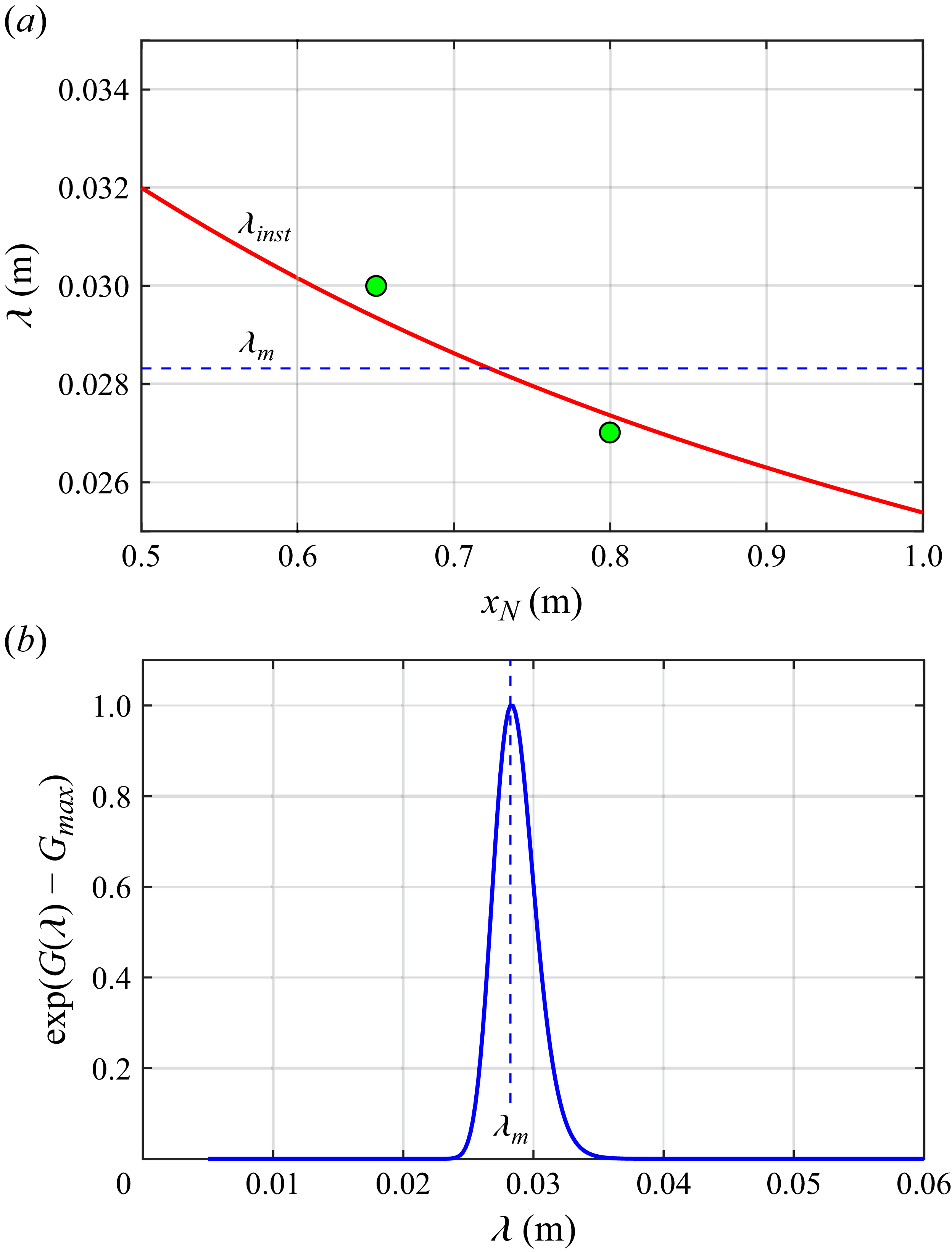
 ∘
 xN∈[0.50,1.00]m
 β/α=1.5
 λm

 Δϕ=70∘
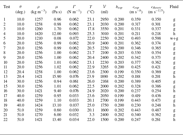
 θ
 ρ
 μ
 Γ
 T
 V
 cexp
 bexp
 rN=ctb
 ctheory
 b=1/5


 V=2300ml
 θ=20.4∘
 t=3.5s
 t=10s
 t=15.5s
 t=30.5s
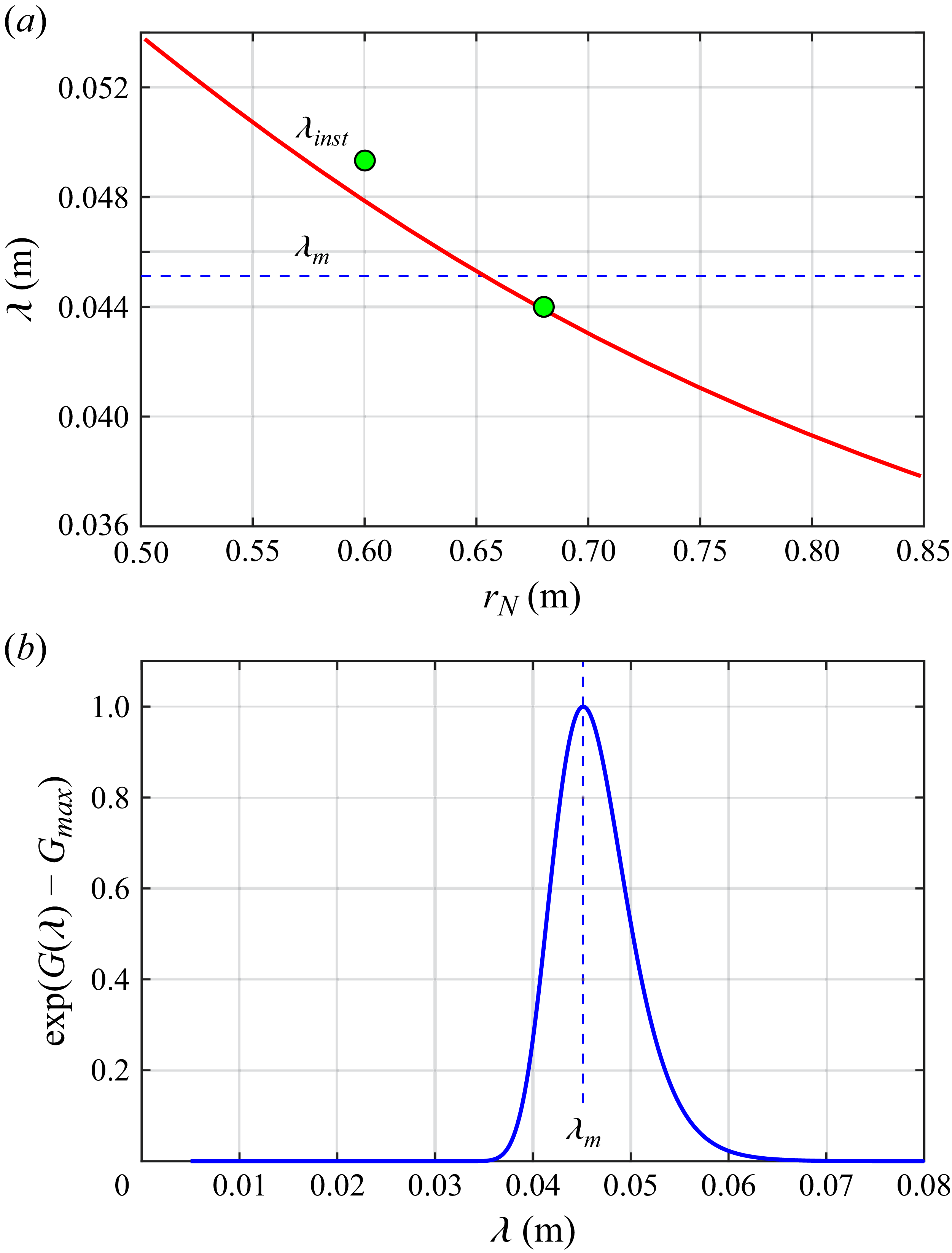
 rN∈[0.50,0.85]m
 β/α=2.8
 λm
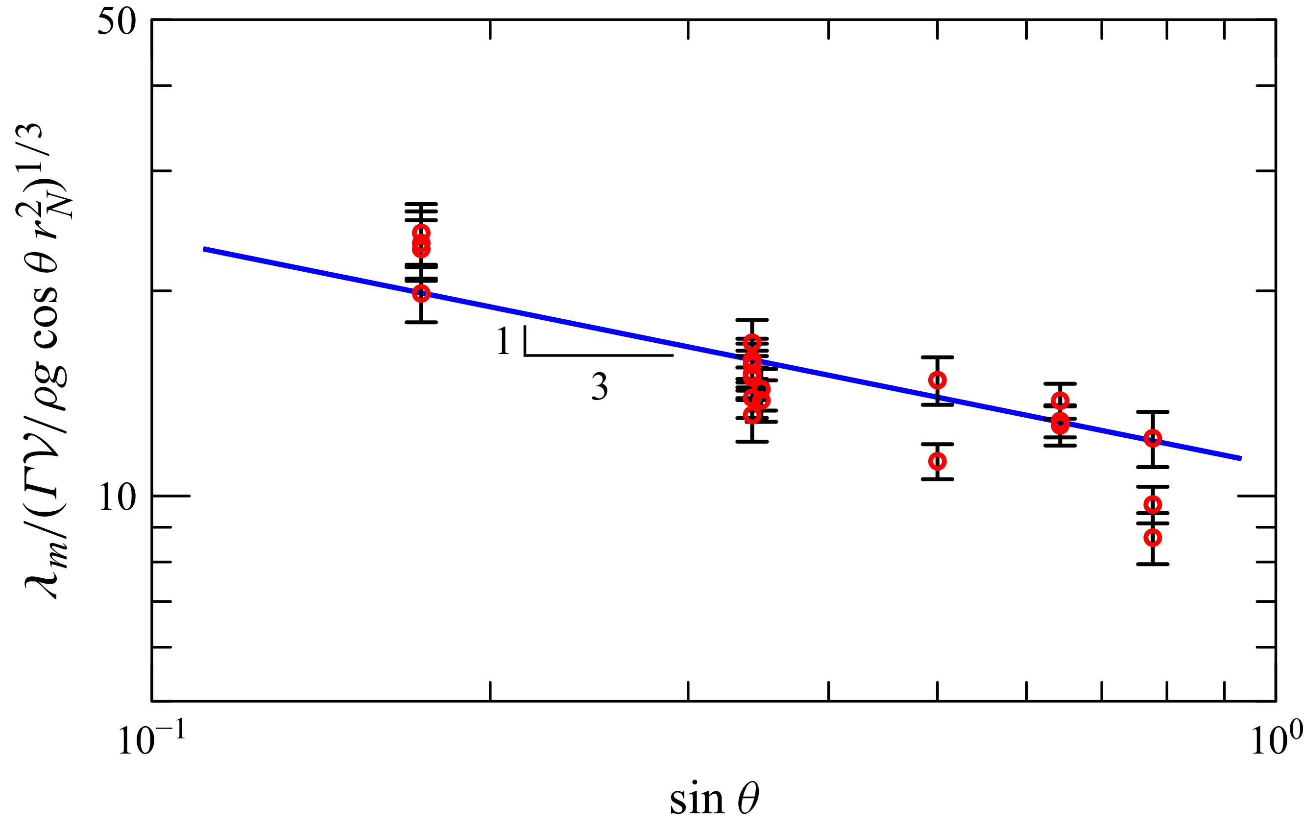
 [ΓV/(ρgcosθrN2)]1/3
 sinθ
 rN2=rN,0rN,1
 (sinθ)−1/3


 Open access

