1 Introduction
Arranging ships or ship-shaped floating bodies in a closely spaced parallel alignment (‘side-by-side’) is necessary in some marine industrial applications, particularly transfer of liquefied natural gas from a floating production vessel to a carrier. This practice creates a long, narrow gap between the vessels, which supports highly resonant free surface motions at particular frequencies. As for any highly resonant system, the amplitude of the response depends on the system damping, and the resonance may be excited in a linear or nonlinear fashion. For industrial applications, the amplitude of the resonance during operations (moderate sea states) may be important in its own right, or due to its coupling with vessel motion.
It is well established that linear potential flow theory can predict resonant frequencies and mode shapes well (Molin Reference Molin2001; Sun, Eatock Taylor & Taylor Reference Sun, Eatock Taylor and Taylor2010; Molin et al. Reference Molin, Zhang, Huang and Remy2018). However, potential flow theory typically overpredicts experimentally determined resonant amplitudes of gap responses (e.g. Buchner, Van Dijk & De Wilde Reference Buchner, Van Dijk and De Wilde2001) unless artificial dissipation is added (e.g. Chen Reference Chen2005). Sources of this amplitude discrepancy are generally believed to be viscous effects and perhaps effects associated with the nonlinear free surface condition. The latter effect was investigated numerically by Feng & Bai (Reference Feng and Bai2015), who found only very slight reductions in the amplitude of the resonant response even for rather steep incoming waves.
Thus, more effort has been focused on viscous dissipation. In an early experimental study of the gap problem, Molin et al. (Reference Molin, Remy, Kimmoun and Stassen2002) estimated the energy losses due to wall friction and flow separation at the (square) bilge for waves propagating in a long narrow channel; wall friction being approximately 15 % of the total. Kristiansen & Faltinsen (Reference Kristiansen and Faltinsen2012) and Fredriksen, Kristiansen & Faltinsen (Reference Fredriksen, Kristiansen and Faltinsen2015) created two-dimensional (2D) hybrid potential flow Navier–Stokes (NS) solver models to try to incorporate losses due to separation from the sharp bilges of catamaran boxes in forced heave and wave-excited heave and roll, and found good agreement with response curves from experiments. Faltinsen & Timokha (Reference Faltinsen and Timokha2015) and Tan et al. (Reference Tan, Lu, Tang, Cheng and Chen2017) developed methods based on hydraulic arguments and calibration with 2D experimental data to modify potential flow solvers to correctly incorporate viscous losses.
Experimental studies have been crucial in the above work but largely focused on 2D geometries. Three-dimensional (3D) gap resonance experiments have been performed by Molin et al. (Reference Molin, Remy, Camhi and Ledoux2009), Perić & Swan (Reference Perić and Swan2015) and Chua et al. (Reference Chua, de Mello, Malta, Vieira, Watai, Ruggeri, Eatock Taylor, Nishimoto and Choo2018), amongst others. Recently Zhao et al. (Reference Zhao, Wolgamot, Taylor and Eatock Taylor2017) conducted 3D experiments in transient wave groups, for vessels with round and square bilges. In both cases substantial damping in addition to radiation damping was clearly present, and for the round bilge cases it was suggested that the damping was almost entirely due to laminar boundary layers.
NS solvers have been extensively applied to gap resonance in two dimensions, but less so in three, where the computational demand is greater. Feng et al. (Reference Feng, Bai, Chen, Qian and Ma2017) simulated regular waves interacting with the square bilge version of the 3D model tested by Molin et al. (Reference Molin, Remy, Camhi and Ledoux2009), and found reasonable agreement with experimental response curves (generated from irregular wave tests). For each frequency considered, it was found necessary to run 20–50 wave periods, to ensure that steady state was reached. When the bilges were rounded, Feng et al. (Reference Feng, Bai, Chen, Qian and Ma2017) found that the response curves obtained from the NS solver agreed well with linear potential flow theory. A notable difference between this case and Zhao et al. (Reference Zhao, Wolgamot, Taylor and Eatock Taylor2017) was the gap width – the geometries being otherwise similar, the latter featured a gap width around half that of the former, which entails a large change in the relative contribution of viscous and radiation damping.
In this work two transient wave group experiments of Zhao et al. (Reference Zhao, Wolgamot, Taylor and Eatock Taylor2017) are reproduced using an NS solver – this ambitious effort enables comparison of time series rather than averaged responses, and by reducing the simulation time required (compared to using regular waves), increases the numerical resolution that can be used. By simulating one case with linear excitation and one case with frequency doubling, resolution of nonlinear free surface effects is demonstrated. The approach taken also enables a detailed investigation of the nature of the damping, to a resolution not feasible in experiments.
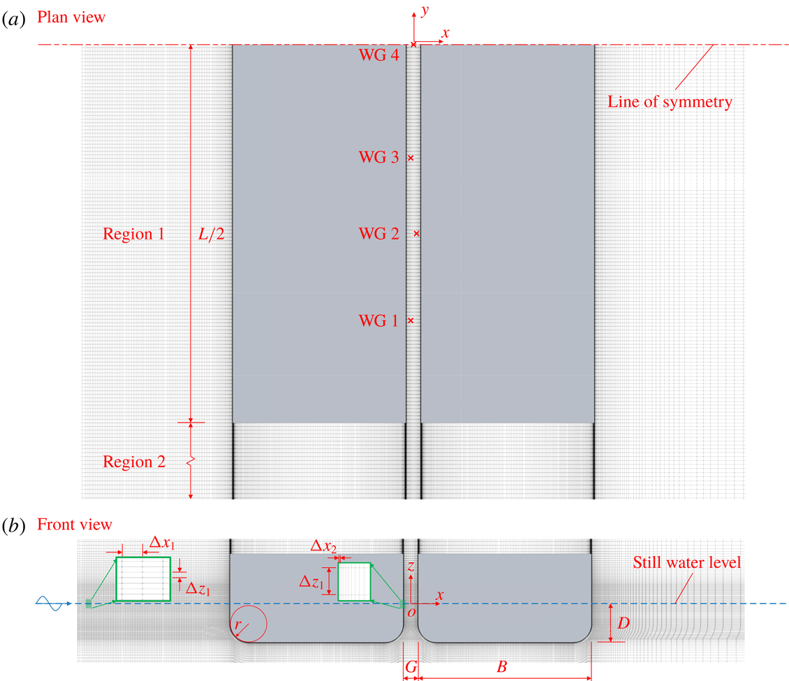
Definition sketch of experimental and numerical (mesh A3) set-ups.

2 Re-creating experiments
In this section, experimental and numerical details of primary importance are presented; more complete information can be found in Zhao et al. (Reference Zhao, Wolgamot, Taylor and Eatock Taylor2017) and Wang et al. (Reference Wang, Draper, Zhao, Wolgamot and Cheng2018), respectively.
2.1 Experimental
Zhao et al.’s (Reference Zhao, Wolgamot, Taylor and Eatock Taylor2017) experiments were carried out in the Deepwater Wave Basin at Shanghai Jiao Tong University. Two identical prismatic boxes of length
 $L=3.333$
m, beam
 $B=0.767$
m and draft
 $D=0.185$
m with rounded bilges of radius
 $r=0.083$
m were used in the experiments. Arranged with long axes parallel, aligned at the fore and aft perpendicular, the boxes formed a narrow gap of width
 $G=0.067$
m (as indicated in figure 1). The fixed boxes were subjected to long-crested transient wave groups incident from the beam. Seven wave gauges (WGs) were placed symmetrically along the gap: WG 4, central; WG 3 and WG 5, 0.50 m offset; WG 2 and WG 6, 0.833 m offset; and WG 1 and WG 7, 0.45 m from the gap ends. In this work two of the wave groups are considered, here called case A and case B (set I and set VIA, respectively, in Zhao et al. (Reference Zhao, Wolgamot, Taylor and Eatock Taylor2017)). Both wave groups had a maximum surface elevation of approximately 50 mm: for case A the spectral peak frequency of
 $f_{p}=1.015$
Hz (peak wavelength
 $\unicode[STIX]{x1D706}_{p}=1.5$
m) coincided with the first gap mode; while for case B the spectral peak frequency was halved to
 $f_{p}=0.508$
Hz (
 $\unicode[STIX]{x1D706}_{p}=6$
m). The input wave spectrum used for both cases was Gaussian in frequency.
2.2 Numerical
Simulations were carried out in a 3D numerical wave tank (NWT) shown in figure 1 solving the two-phase incompressible NS equations with volume-of-fluid free surface tracking. The NWT was established using OpenFOAM and the governing equations solved using a finite volume method discretised on a structured mesh. The origin of the NWT was positioned at the mean free surface at the centre of the gap, with
 $x$
the direction of wave propagation and
 $z$
positive upwards. The toolbox waves2Foam (Jacobsen, Fuhrman & Fredsøe Reference Jacobsen, Fuhrman and Fredsøe2012) was used for generation of incident waves and absorption of reflected waves using relaxation zones at both ends of the NWT. The experimental incident wave groups were re-created with considerable accuracy in the NWT using an iterative method (see figure 2 and Wang et al. (Reference Wang, Draper, Zhao, Wolgamot and Cheng2018) for details). The size of the NWT must be minimised; the lengths of the NWT for cases A and B were chosen as
 $8.0\unicode[STIX]{x1D706}_{p}$
and
 $5.2\unicode[STIX]{x1D706}_{p}$
, respectively, to allow wave propagation and absorption upstream and downstream of the boxes, while the water depths were
 $\unicode[STIX]{x1D706}_{p}$
and
 $0.58\unicode[STIX]{x1D706}_{p}$
(which fulfil the deep-water condition). Sidewalls were set at
 $y=4L$
and
 $y=12L$
for cases A and B, respectively, to limit wave reflection.
Comparison of numerical and experimental incident wave groups for cases A and B.

Knowledge of Zhao et al.’s (Reference Zhao, Wolgamot, Taylor and Eatock Taylor2017) experiments informed the selection of mesh parameters shown in figure 1. The maximum Reynolds number here is
 $Re=\unicode[STIX]{x1D714}\unicode[STIX]{x1D702}_{o}^{2}/\unicode[STIX]{x1D708}\simeq 2.3\times 10^{4}$
, where
 $\unicode[STIX]{x1D714}$
is the first resonant frequency,
 $\unicode[STIX]{x1D708}$
the kinematic viscosity and
 $\unicode[STIX]{x1D702}_{o}$
the amplitude of free surface motion at the centre of the gap, with a maximum value of around 0.06 m. For oscillatory flow over a smooth plane wall, turbulence first appears at
 $Re\simeq 10^{5}$
(Jensen, Sumer & Fredsøe Reference Jensen, Sumer and Fredsøe1989). However, the possibility of flow separation from the rounded bilge must also be considered. Here the maximum local Keulegan–Carpenter number
 $KC=2\unicode[STIX]{x03C0}\unicode[STIX]{x1D702}_{o}/2r$
for flow around the rounded bilge is approximately 2.3. For flow around a cylinder Sumer & Fredsøe (Reference Sumer and Fredsøe2006) give flow regimes for a limited subset of (
 $KC$
–
 $Re$
) space; for
 $Re\simeq 10^{3}$
there is no separation for
 $KC<1.1$
. Given that the present geometry is not a cylinder, and the oscillatory flow is transient, the
 $KC$
and
 $Re$
regimes for this problem make it plausible that laminar boundary layers dominate the damping in this case, and the mesh design is based around this hypothesis. The thickness of a Stokes boundary layer based on the parameters above is around
 $\unicode[STIX]{x1D6FF}_{0.99}=4.6\sqrt{2\unicode[STIX]{x1D708}/\unicode[STIX]{x1D714}}\simeq 2.5$
mm for the first mode. In light of this, four meshes A1–A4 with near-wall cell width normal to the box walls
 $\unicode[STIX]{x0394}x_{2}$
equal to 2.0, 0.4, 0.1 and 0.05 mm were used to simulate case A. The adjacent cells expand away from the wall to take account of the fact that the near-wall velocity gradient is much larger than that near the gap centre. The other mesh dimensions are essentially the same for the four cases. The mesh size along the wave propagation direction
 $\unicode[STIX]{x0394}x_{1}$
is chosen to achieve 200 cells per peak wavelength to resolve propagating incident waves. The vertical cell height
 $\unicode[STIX]{x0394}z_{1}$
is chosen to ensure the aspect ratio (i.e.
 $\unicode[STIX]{x0394}z_{1}/\unicode[STIX]{x0394}x_{2}$
) remains small, so that 20 cells per wave height are used for mesh A1 while 50 cells per wave height are used for meshes A2–A4. Along the gap direction, the cell width in the gap (region 1 in figure 1(a), from the mid-ship position
 $y=0$
to the gap end
 $y=-L/2$
) is chosen to give 60 cells per ‘wavelength’ of the seventh mode shape. The cell width outside the gap (region 2 in figure 1(a), from the gap end to the sidewall) expands gradually away from the gap end. Given that attached laminar boundary layers are expected, a symmetry boundary condition was applied at the mid-ship plane (see figure 1
a) to reduce the computational cost. However, due to the two-scale nature of this problem, in which surface wavelength and boundary layer scales are resolved simultaneously, the number of cells is still extremely large, which renders the 3D simulations very demanding (e.g. mesh A3 has 48.1 million cells and the simulation requires approximately 1 million CPU hours, computed using 720 cores on a Cray XC40 supercomputer with 2.6 GHz Intel Xeon E5-2690 v3 ‘Haswell’ CPUs). For robustness, the time step of the simulations was chosen to be runtime adaptive with maximum Courant number not exceeding 0.5 (chosen based on experience). Although the gap is relatively narrow, surface tension is not represented numerically, since the Bond number
 $B_{o}=gL^{2}\unicode[STIX]{x1D70C}/T_{s}\simeq 1.5\times 10^{6}$
(where
 $g$
and
 $\unicode[STIX]{x1D70C}$
are gravitational acceleration and fluid density, respectively, and
 $T_{s}=0.073~\text{N}~\text{m}^{-1}$
is the surface tension). This is well above the range where surface tension is important, according to Faltinsen & Timokha (Reference Faltinsen and Timokha2009).
Boundary layer profiles in the gap at various phases over a nominal cycle
 $T$
(from 8.12 s to 9.10 s) computed numerically (thin lines) and using (2.1) (circles) for meshes (a) A1 and (b) A3, at
 $y=0$
,
 $z=-0.43D$
.

Response at gap centre for meshes A1–A4 (a) and that from mesh A3 compared to Zhao’s experiments (b) for case A (linear excitation). The time axes are as in figure 2.

2.3 Kinematics: linear excitation
The same incident crest-focused wave group corresponding to case A has been used to excite gap motions for meshes A1–A4. The excitation resulting from this wave group is mostly linear because the frequency content of the wave group overlaps with the natural frequencies of the dominant gap modal responses. Based on the arguments above, the near-wall velocity profile should resemble a Stokes boundary layer for oscillatory flow over an infinite flat plate. Here, however, there are multiple oscillation frequencies, all associated with time-varying amplitude and the hull is finite and rounded (though
 $r\gg \unicode[STIX]{x1D6FF}_{0.99}$
). To compare the boundary layer profile computed in the vertical part of the gap in the NWT to this theory, a velocity-based time-dependent pressure gradient is used to numerically solve the Stokes equation,
 $$\begin{eqnarray}\unicode[STIX]{x0394}p(t)=-\unicode[STIX]{x1D70C}\frac{\unicode[STIX]{x2202}u}{\unicode[STIX]{x2202}t}+\unicode[STIX]{x1D707}\frac{\unicode[STIX]{x2202}^{2}u}{\unicode[STIX]{x2202}x^{2}}+\unicode[STIX]{x1D70C}g,\end{eqnarray}$$
where
 $u$
represents vertical fluid velocity. To calculate the vertical velocity profile away from a point on the wall in the straight part of the gap, at a depth which the free surface does not reach, the velocity-based pressure gradient
 $\unicode[STIX]{x0394}p(t)$
taken from the full 3D simulation at
 $0.05G$
away from the wall is applied in (2.1) (this sampling point is close to the wall but still outside the boundary layer). Agreement between the theoretical solution and the 3D simulation results becomes better as the near-wall mesh is refined, such that A3 and A4 give excellent agreement; the results of A1 and A3 for the point
 $(-G/2,0,-0.43D)$
based on
 $\unicode[STIX]{x0394}p(t)$
from
 $(-0.9G/2,0,-0.43D)$
are shown in figure 3. Similar results apply for other points.
Time series of free surface elevation at the centre of the gap for meshes A1–A4 are compared in figure 4(a). The phases from meshes A2, A3 and A4 agree well, while A1 leads the other three slightly. In terms of amplitude, the gap responses decay more swiftly as the near-wall mesh is refined. It is clear that, after the initial ‘excitation’ stage the responses of A1
 ${>}$
A2
 ${>}$
A3
 $\simeq$
A4. Based on figures 3 and 4(a), we conclude that convergence is achieved for mesh A3. Thus, in figure 4(b) the responses at the centre of the gap computed using A3 are compared to the experimental measurements of Zhao et al. (Reference Zhao, Wolgamot, Taylor and Eatock Taylor2017). The agreement between the simulations and experiments is good. The slight overpredictions which occur periodically arise because multiple modes are excited (see § 3.1), each with small errors in amplitude and phase (due to the numerical incident waves, experimental set-up, etc.). Such errors are noticeable at times in the response when multiple modes reinforce or cancel.
Snapshots of numerically computed response wave field for mesh A3 (in the region
 $2.5~\text{m}<x<8.5~\text{m}$
,
 $-4.0~\text{m}<y<0~\text{m}$
) captured at different times. Note that the vertical axis is stretched, such that 1 unit in the vertical equals 5 units in the horizontal, to more clearly show the free surface motions. To this end, the boxes are shown as transparent.

Comparison of experimentally and numerically (mesh B3) determined harmonic responses: (a) long-wave difference component; (b) first harmonic; (c–f) second harmonic; (g) third harmonic; and (h) fourth harmonic, with scaled envelope squared of the second harmonic (dashed grey lines). The time axes are as in figure 2.

The full interaction of the wave group with the boxes is shown in supplementary movie 1 (available at https://doi.org/10.1017/jfm.2019.115). Snapshots of the interaction at
 $t=0$
and 1.8 s are shown in figure 5. The large wave crest is essentially unaltered at the edge of the figure (downstream and outside the boxes), whereas waves are almost absent downstream and behind the boxes in region 1 (see figure 1). This illustrates the strongly directional nature of the waves scattered from the boxes – most energy is reflected back up-wave and a small amount excites free surface modes within the gap. The ‘near-trapped’ wave energy then causes the fluid in the gap to oscillate within the side-by-side system, slowly leaking wave energy out into the external wave field. As a result, the gap oscillations persist long after the incident group has passed, as shown in supplementary movie 1. Higher-frequency scattered waves are also evident radiating from the gap in figure 5(b), and upstream of the leading box.
2.4 Kinematics: nonlinear excitation
Meshes B1 and B3, identical to A1 and A3 in the gap region, were used to compute responses to two wave groups for case B, shown in figure 2 and labelled crest-focused and trough-focused (in which each frequency component in the linear spectrum of the crest-focused wave is phase-shifted by
 $180^{\circ }$
). For these wave groups the gap modes are excited nonlinearly through quadratic wave–wave–structure interactions. As in the experiments, the two-phase runs allowed odd and even harmonics to be extracted using the phase inversion method of Fitzgerald et al. (Reference Fitzgerald, Taylor, Eatock Taylor, Grice and Zang2014), with the results presented in figure 6 for mesh B3. There are some discrepancies between the numerical and experimental results for the (very small) long-wave difference component when
 $t<1.6$
s but the agreement is better from
 $t=1.6$
s onwards. The numerical and experimental first-, second- and third-order harmonics are in good agreement. As for case A, periodically the agreement deteriorates; seen in this light the third harmonic result is remarkable. The agreement for the fourth harmonic is not as good as for the other harmonics. However, assuming there is a generalised Stokes-type perturbation expansion for the gap responses, it is possible to match the envelope of the fourth harmonic component by squaring the envelope of the second harmonic (calculated as
 $\sqrt{\unicode[STIX]{x1D702}_{2}^{2}+\unicode[STIX]{x1D702}_{2H}^{2}}$
, where
 $\unicode[STIX]{x1D702}_{2H}$
is the Hilbert transform of the second harmonic free surface elevation
 $\unicode[STIX]{x1D702}_{2}$
) and then fitting the measured envelope of the fourth harmonic component by a least-squares method. Figure 6(h) shows that the extracted fourth harmonic fits the scaled squared envelopes of the second harmonic quite well, demonstrating that the numerical results are self-consistent. These results represent a highly successful application of an NS solver to a problem with linear viscous dissipation but nonlinear free surface effects, both of which must be resolved to achieve satisfactory results. NS solvers have previously been used to derive second harmonic responses around non-resonant structures such as cylinders in relatively steep waves (Paulsen et al.
Reference Paulsen, Bredmose, Bingham and Jacobsen2014). Here the strength of the second harmonic response is much stronger; even in waves which are not very steep, the second harmonic responses are as large as the first.
Non-dimensional damping coefficient for each mode versus frequency (discontinuous axis) for each numerical simulation compared to experimental results. The modes shown are modes 1, 3 and 5 (from left to right). The grey dashed vertical lines and values above represent the resonant frequencies obtained from the potential flow software DIFFRACT.

3 Damping analysis
3.1 Global damping
Owing to the transient nature of the incident wave group, the gap response can be conceptualised as occurring in two stages, i.e. the excitation stage when the incident waves drive the gap motions, and the decay stage, when the incident waves have passed and the gap motion is a pure oscillatory decay. If the total damping in this decay stage is linear, the free surface elevations should be well represented by a series of decaying sinusoids with frequencies corresponding to the gap modes, as in Zhao et al. (Reference Zhao, Wolgamot, Taylor and Eatock Taylor2017). Thus
 $$\begin{eqnarray}\unicode[STIX]{x1D702}(t)=\mathop{\sum }_{n}A_{n}\sin (\unicode[STIX]{x1D714}_{n}t+\unicode[STIX]{x1D719}_{n})\exp [-\unicode[STIX]{x1D714}_{n}\unicode[STIX]{x1D709}_{n}t],\end{eqnarray}$$
where
 $f_{n}=\unicode[STIX]{x1D714}_{n}/2\unicode[STIX]{x03C0}$
is the resonant frequency of the
 $n\text{th}$
mode,
 $\unicode[STIX]{x1D709}_{n}$
the normalised modal damping, and
 $A_{n}$
and
 $\unicode[STIX]{x1D719}_{n}$
the amplitude and phase at the start of the time window. The method of Kumaresan & Tufts (Reference Kumaresan and Tufts1982) performs well in estimating the parameters of exponentially damped sinusoids for short data records, and is used here to calculate the modal parameters using free surface elevation time series at a number of points in the gap, assuming
 $f_{n}$
and
 $\unicode[STIX]{x1D709}_{n}$
are independent of position along the gap, while
 $A_{n}$
and
 $\unicode[STIX]{x1D719}_{n}$
vary with position (reflecting the modal spatial structure). The effectiveness of applying this method to the gap resonance problem has been demonstrated in Zhao et al. (Reference Zhao, Wolgamot, Taylor and Eatock Taylor2017). Choosing a 20 s time window of
 $t=[9,29]$
s, the analysis is conducted for the experimental and numerical results for cases A and B. The resonant frequencies and corresponding damping coefficients are shown in figure 7.
Figure 7 suggests that the first resonant frequency identified from the numerical results matches the experimental value more closely than potential flow theory for the first mode, while the opposite is true for the higher modes. Nevertheless, the frequency agreement in all cases is quite good (within
 $1\,\%$
). The modal damping values are of primary interest, and approach the experimental levels from below as the mesh is gradually refined and the boundary layer resolved. For the finer meshes A3 and A4 the damping is in satisfactory agreement with the experimental values, despite being slightly smaller. Part of this error may be attributable to the temperature dependence of viscosity – in the simulations
 $\unicode[STIX]{x1D707}=1000~\unicode[STIX]{x03BC}\text{Pa}~\text{s}$
, while temperatures in the Shanghai basin during the tests were
 $17\,^{\circ }\text{C}$
, giving
 $\unicode[STIX]{x1D707}=1080~\unicode[STIX]{x03BC}\text{Pa}~\text{s}$
. Damping values for each mode are similar for cases A and B, while the third mode is generally underpredicted more than the others.
From the numerical point of view, a coarse mesh usually induces larger unphysical diffusion than a finer mesh, so it is common for fluid damping to be overpredicted when mesh refinement is inadequate. Here, however, it appears that the damping induced by wall friction dominates any unphysical diffusion. In this case the diffusion should be small, since the structured mesh in the gap follows the curvature of the walls and the convection term is small since the gap flow is Stokes-like. At this point, note should be made of the work of Kristiansen & Faltinsen (Reference Kristiansen and Faltinsen2012), who demonstrated convergence of gap responses by varying the number of uniform cells across the gap and concluded that gap responses were not sensitive to mesh refinement in the gap for their 2D geometry with square bilges. However, for the geometry with rounded bilges in the present study, it is emphasised that the gap responses can only be predicted with good accuracy when the boundary layer scale is resolved properly.
3.2 Local damping
While the ‘global’ damping of the computed free surface motions appears satisfactory, the advantage of numerical simulations is that the flow field can be interrogated in detail. It is of interest to determine whether the local fluid behaviour supports the supposition that the viscous damping is due to laminar boundary layers. Contours of normalised vorticity have been computed and examined, though they are not shown here, as no visible vortex shedding occurs from the bilges throughout the simulation, while small vortex shedding occurs from the sharp corners at the gap ends during the excitation phase. To more quantitatively assess the nature of the dissipation, the viscous dissipation is computed for various control volumes. The rate of energy dissipation by the action of viscosity per unit time in a control volume
 $V$
can be calculated as (Whitham Reference Whitham and Rosenhead1963)
 $$\begin{eqnarray}{\dot{E}}_{v}=\frac{1}{2}\int _{V}\unicode[STIX]{x1D707}(e_{xx}^{2}+e_{yy}^{2}+e_{zz}^{2}+2e_{yz}^{2}+2e_{zx}^{2}+2e_{xy}^{2})\,\text{d}V,\end{eqnarray}$$
where
 $e_{xx}=2(\unicode[STIX]{x2202}u_{x}/\unicode[STIX]{x2202}x)$
,
 $e_{xy}=\unicode[STIX]{x2202}u_{y}/\unicode[STIX]{x2202}x+\unicode[STIX]{x2202}u_{x}/\unicode[STIX]{x2202}y$
, etc. are the rate-of-strain components. To attempt to separate the possible viscous dissipation contributions from wall friction and flow separation, two control volumes are used. Control volume
 $V_{1}$
surrounds the boxes with
 $x$
bounds
 $[-1.25,1.25]\times (G/2+B)$
,
 $z$
extending from the NWT floor to the time-varying free surface
 $\unicode[STIX]{x1D702}$
and
 $y$
out to
 $0.56L$
. Control volume
 $V_{2}$
is a thin layer surrounding the boxes with a thickness
 $\unicode[STIX]{x1D6FF}=3$
mm (the blue area in cross-section shown in figure 8 projecting along the gap). The viscous dissipation rates in these control volumes are compared in figure 8. It is found that the largest difference between
 $V_{1}$
and
 $V_{2}$
at any time in the decay stage is less than 8 %, and the cumulative difference in viscous dissipation (integrating over time from
 $t=9$
s to
 $t=29$
s) is less than 2 %, which means that nearly all of the viscous dissipation occurs in a thin layer surrounding the boxes, suggesting that laminar boundary layers are indeed the dominant damping contribution.
Dissipation rate time series for control volumes
 $V_{1}$
and
 $V_{2}$
, mesh A3, case A and (inset) cross-section diagram of control volume
 $V_{2}$
, for which
 $\unicode[STIX]{x1D6FF}=3$
mm.

Having computed the viscous dissipation rate, it is possible to use this to compute (at least approximately) the expected decay rate of the free surface in the gap and compare to that found in the simulation, on a modal basis. It is therefore necessary to obtain estimates of the average rate of energy loss from the oscillating system (
 ${\dot{E}}_{n}$
) and the amount of energy stored in the oscillating system (
 $E_{n}$
) for each mode (per unit modal amplitude squared), which are related to the non-dimensional damping for each mode by
 $$\begin{eqnarray}\unicode[STIX]{x1D709}_{n}\propto \frac{{\dot{E}}_{n}}{E_{n}},\end{eqnarray}$$
(when the damping is small) assuming that the gap decay is well described by (3.1). The total rate of energy loss is assumed to be the sum of radiation and viscous contributions, i.e.
 ${\dot{E}}_{n}={\dot{E}}_{r}^{n}+{\dot{E}}_{v}^{n}$
. As the total energy of the oscillating system
 $E_{n}$
should be the same for viscous or inviscid calculations, we can write
 $$\begin{eqnarray}\unicode[STIX]{x1D709}_{n}={\dot{E}}_{n}\times \frac{\unicode[STIX]{x1D709}_{r}^{n}}{{\dot{E}}_{r}^{n}},\end{eqnarray}$$
where
 $\unicode[STIX]{x1D709}_{r}^{n}$
and
 ${\dot{E}}_{r}^{n}$
are the damping coefficient and rate of dissipation, respectively, caused by radiation by mode
 $n$
. These have been calculated using the linear potential flow software DIFFRACT, which is convenient as the different modal contributions are computed separately. The radiated wave field is obtained by subtracting the scattered wave field from a large box of width
 $(2B+G)$
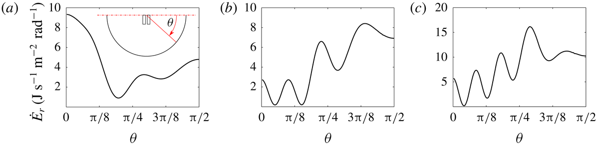
from the scattered field for the gap problem. This approach takes advantage of the narrowness of the gap, and is evidently deficient close to the ends of the gap, but otherwise produces smooth, symmetrical radiated wave fields. For each mode, the rate of energy radiation to infinity is computed using the radiated field at large radius from the boxes – radiation patterns are shown in figure 9. It is interesting that mode 1 radiates most strongly perpendicular to the gap (or along the NWT) while the other modes radiate most strongly around the direction along the gap (i.e. out the ends of the gap).
Radiation pattern, in terms of energy loss per unit modal amplitude squared per radian, from gap mode 1 (a), mode 3 (b) and mode 5 (c) determined using linear potential flow software DIFFRACT in an unbounded domain. The definition sketch of
 $\unicode[STIX]{x1D703}$
is shown in (a) and
 $\unicode[STIX]{x1D703}=\unicode[STIX]{x03C0}/2$
is along the gap direction.

To complete the analysis, the viscous dissipation rates shown in figure 8 must be separated into modal contributions. Given the form of (3.2) and that the velocity in the gap is in a form similar to (3.1), with spatial decay of the velocity towards the wall, it is clear that for each mode there are dissipation rate contributions which are purely decaying in time, and those which oscillate at twice the gap mode frequencies. In addition, there are sum and difference frequency terms (cross-mode terms) and terms at the gap oscillation frequencies caused by the time dependence of
 $V$
in (3.2) (due to the varying run-up on the box). Were the oscillations constant-amplitude instead of decaying, time-integrating the dissipation rate to recover the average or total dissipation would remove all of the oscillatory terms, leaving only the mean. In this case we say simply that we expect the pure decay terms to dominate. As the double-frequency dissipation rate terms occur in the same proportion as the pure decay terms, it is possible to fit the double-frequency terms using the same method as applied above (after isolating them with a bandpass filter), and use the relative amplitudes to divide the pure decay dissipation rate signal into modal contributions. Once the modal components of viscous dissipation rate are obtained, the global damping coefficients for each mode can be calculated according to (3.4).
The analysis described above is carried out on the viscous dissipation rate time series from
 $t_{0}=9$
s onwards for mesh A3. The amplitude spectrum of the viscous dissipation rate is obtained using the fast Fourier transform as shown in figure 10(a), while the high-pass and low-pass time series are shown in figure 10(b). Applying the method of Kumaresan & Tufts (Reference Kumaresan and Tufts1982) to the high-pass signal, it is found that the reconstructed signal gives a very good approximation of the original high-pass signal (see figure 11
a). The modal frequencies
 $\unicode[STIX]{x1D714}_{vh}^{n}$
and non-dimensional ‘damping’
 $\unicode[STIX]{x1D709}_{vh}^{n}$
determined from the double-frequency viscous dissipation rate terms closely match those for the free surface elevations over the same period (within
 $0.1\,\%$
for frequencies and
 $3\,\%$
for damping), which means the coupling between different modes is indeed weak as expected. The low-pass viscous dissipation rate signal should contain modal signals with the same modal rates of decay and proportionality coefficients
 $$\begin{eqnarray}\unicode[STIX]{x1D6FC}_{n}=\frac{{\dot{E}}_{vh}^{n}(t_{0})}{{\dot{E}}_{vh}(t_{0})}\end{eqnarray}$$
as the high-pass signal. Thus, the dominant term in the low-pass signal can be expressed as the sum of three pure decay curves (
 $n=1,3,5$
) in the appropriate ratio (
 $\unicode[STIX]{x1D6FC}_{n}$
) and scaled by a constant
 $C$
as
 $$\begin{eqnarray}{\dot{E}}_{v}=\mathop{\sum }_{n}C\unicode[STIX]{x1D6FC}_{n}\exp [-2\unicode[STIX]{x1D714}_{vh}^{n}\unicode[STIX]{x1D709}_{vh}^{n}t].\end{eqnarray}$$
A numerical fit based on a least-squares method gives very good agreement with the original signal shown in figure 11(b), with the coefficient of determination
 $R^{2}=0.96$
, meaning that
 ${\dot{E}}_{v}^{n}$
has been determined.
Amplitude spectrum (a), and high-pass and low-pass time series (b) of viscous dissipation rate from
 $t=-3$
to
 $t=29$
s. In (a), double-frequency peaks corresponding to the three main gap modes can clearly be seen between 2 and 2.5 Hz, and the red dashed line represents the cut-off frequency for the filters.

Numerical fit of high-pass (a) and low-pass (b) viscous dissipation rate time series, using the method of Kumaresan & Tufts (Reference Kumaresan and Tufts1982) and a least-squares method, respectively.

Values of
 $\unicode[STIX]{x1D709}\times 10^{3}$
determined from ‘global’
 $\unicode[STIX]{x1D702}$
(corresponding to the damping coefficients in figure 7) and ‘local’
 $\unicode[STIX]{x1D707}$
analyses.

Using (3.4) we arrive at the global damping results shown in table 1, where
 $\unicode[STIX]{x1D709}_{\unicode[STIX]{x1D702}}$
is the global damping derived from the free surface elevations and shown in figure 7 and
 $\unicode[STIX]{x1D709}_{\unicode[STIX]{x1D707}}$
is the global damping derived using the dissipation calculation. The comparison is reasonable (in light of the caveats discussed below), confirming the consistency of these results, and the conclusion that the viscous damping is dominated by laminar boundary layer behaviour.
It should be emphasised that producing a global damping value from radiation and viscous contributions in the manner undertaken here involves several approximations, some mentioned above, and some discussed here. Using (3.1) to represent the gap motions works well because each mode may be described by a complex resonance (see e.g. Meylan & Eatock Taylor Reference Meylan and Eatock Taylor2009), though using the radiation damping behaviour from a single (real) frequency is not a rigorous application of this theory; ideally complex frequency calculations would be used. Secondly, the radiation behaviour in the NWT and potential flow are assumed to be the same. As the sidewalls of the NWT are reflective boundaries (while the ends are absorbing), this would tend to reduce the effective radiation damping compared to an unbounded domain potential flow analysis. However, numerical tests with a domain of larger width for mesh A1 did not yield larger damping values. In this case it is important to consider numerical propagation of the radiated wave, which is more than an order of magnitude smaller in amplitude than the gap oscillation or incident wave. As the vertical mesh resolution is optimised for propagation of the incident wave, it may be inadequate to correctly capture propagation of the radiated wave. This difference in scales therefore means that (unphysical) numerical damping of the wave radiated out of the gap reduces the effect of the reflective walls. The effect of the walls is therefore considered minor.
4 Conclusions
In this work numerical solutions of the Navier–Stokes equations have been shown to compare favourably with experimentally observed gap response time series, including higher harmonics, for (we believe) the first time. This is also an excellent test of the possibility of resolving wave and (laminar) boundary layer scale processes in the same simulation, as the amplitude of the resonant response for a narrow gap depends critically on the viscous dissipation, the nature of which cannot feasibly be determined in wave basin tests. Interrogation of the flow field has found that nearly all the viscous dissipation is confined to a thin layer surrounding the boxes, meaning the contribution from flow separation is negligible and wall friction is the main source of damping. Further, the viscous dissipation in the boundary layer has been computed, separated into modes and added to the modal radiation damping contribution to produce modal global damping coefficients in reasonable agreement with those measured in the simulation at the free surface, which are themselves in fairly good agreement with the experimental values.
In contrast to the finding of Kristiansen & Faltinsen (Reference Kristiansen and Faltinsen2012) that the 2D gap response with square bilges is not sensitive to the mesh in the gap, it has been shown that the cell width normal to the wall in the gap is crucial in determining the amplitude response of each of the gap modes for the 3D gap resonance problem with round bilges at laboratory scale. With a sufficiently fine mesh, the numerical near-wall boundary layer can be well predicted by solving a local Stokes equation driven by the time-varying pressure taken at a position near the wall in the gap but still outside the boundary layer.
Given the success of reproducing higher harmonics using the NS solver, it is expected that even higher harmonics could be well predicted if the mesh resolution near the free surface is further refined, though their practical significance may be limited. However, quadratic excitation of gap resonance does appear to be a problem of practical relevance.
Ultimately the gap resonance problem has industrial relevance at a substantially larger scale, though model testing remains a crucial tool for the offshore industry and it is vital to understand these tests. As the scale is increased, the boundary layers will inevitably become turbulent; though this is beyond the scale at which laboratory testing is feasible. For sharp corners or bilge keels, separation will occur in the laboratory as well as in the field.
Acknowledgements
This work was supported by the ARC Industrial Transformation Research Hub for Offshore Floating Facilities which is funded by the Australian Research Council, Woodside Energy, Shell, Bureau Veritas and Lloyds Register (grant no. IH140100012). The support in resources provided by the Pawsey Supercomputing Centre with funding from the Australian Government and the Government of Western Australia is acknowledged. The first author acknowledges support from IPRS, APA and Shell–UWA scholarships.
Supplementary movie
Supplementary movie is available at https://doi.org/10.1017/jfm.2019.115.