



1. Introduction
Propagation of a rippled shock wave is a classical and fundamental issue in the field of shock dynamics. The instability of a corrugated shock front is commonly referred to as the D’yakov–Kontorovich (DK) instability, following the seminal instability criteria developed by D’yakov (Reference D’yakov1954) and Kontorovich (Reference Kontorovich1957). Building on Freeman’s piston-driven formulation for rippled shocks (Freeman Reference Freeman1955), which provides an early rigorous proof of unconditional stability for ideal-gas shock fronts, Landau & Lifshitz (Reference Landau and Lifshitz1987) noted that ideal-gas shocks are free of the DK mechanism. It follows that two-dimensional (2-D) rippled shocks in an inviscid ideal gas are asymptotically stable and exhibit oscillatory algebraic decay, as established by classical analyses employing hyperbolic–polar transformations and Laplace methods (Zaidel Reference Zaidel1960; Nikolaev Reference Nikolaev1965; Briscoe & Kovitz Reference Briscoe and Kovitz1968; Ishizaki & Nishihara Reference Ishizaki and Nishihara1997). In particular, the shock-front perturbation decay scales as
 $t^{-3/2}$
(general case) or
 $t^{-1/2}$
(strong-shock limit) in an ideal gas. Explicit formulations for general equations of state and their late-time behaviour have subsequently been derived (Bates Reference Bates2004; Shen et al. Reference Shen, Pullin, Samtaney and Wheatley2021; Calvo-Rivera et al. Reference Calvo-Rivera, Velikovich and Huete2023), providing a consistent baseline for the relaxation of a rippled shock in an unbounded uniform medium.
When a rippled shock interacts with a material interface, refraction generally produces a transmitted shock and a reflected wave. During the refraction, the transmitted shock will inherit initial amplitude and growth rate, and its subsequent evolution can strongly influence downstream wave fields and interface dynamics. This rippled shock–interface interaction occurs widely in applications. For example, in inertial confinement fusion (ICF), a non-uniform driving laser can imprint spatially correlated modulations onto the ablation pressure and the ensuing shock front (Hu et al. Reference Hu, Michel, Davis, Betti, Radha, Campbell, Froula and Stoeckl2016; Campbell et al. Reference Campbell2021). Since ICF capsules contain multiple material interfaces, this multi-interface environment naturally introduces a sequence of rippled shock transmission processes, in which the transmitted shock after each refraction provides the incident condition for the next, making it essential to predict transmitted-shock evolution accurately. These considerations motivate focusing directly on the dynamics of rippled shock transmission across material interfaces.
Nevertheless, shock transmission across a density interface introduces a qualitatively different setting. Refraction changes the background shock strength and wave speed, thereby altering both attenuation rate and oscillation frequency downstream. In addition, the interface provides a boundary that can reflect acoustic perturbations back towards the shock. Therefore, the transmitted-shock evolution depends strongly on the shock–interface distance through acoustic feedback. Most importantly, a transmitted shock generated by refraction is generally not constrained to begin in the conventional initial phase assumed in most shock perturbation formulations: it typically inherits non-zero initial pressure and normal velocity perturbations at the moment of transmission, meaning that the oscillation can start from an arbitrary phase. This phase freedom makes standard initial-phase theories inadequate for predicting transmitted-shock evolution in practical shock–interface transmission problems, and limits the ability to tailor shock corrugations via interface design. Understanding rippled transmitted-shock dynamics is a fundamental and indispensable component for analysing rippled shock–interface interaction involved in ICF where multiple interfaces and repeated transmissions are unavoidable.
The present study addresses a specific but self-contained problem that is not covered by classical isolated-shock theory: the evolution of a transmitted rippled shock that is generated at a material interface and possesses an arbitrary initial phase and non-zero pressure and normal velocity perturbations. This scope distinguishes the present problem from the conventional initial-phase evolution of an isolated rippled shock. The framework developed here combines three elements: the pre-impact evolution of the incident rippled shock, the local initialisation of the transmitted shock at the interface, and the post-transmission analytical prediction. We first formulate a matching model that maps the transmitted-shock initial conditions onto an equivalent isolated-shock evolution. This construction is computationally simple but is shown to be reliable only in the early stages. We then develop a general analytical model by linearising the post-transmission region and reducing the pressure perturbation dynamics to the Klein–Gordon equation. The resulting Bessel series solution indicates that if the transmitted-shock wave itself carries non-zero initial pressure or normal velocity perturbations, then the even-order terms in the series are crucial. In contrast, traditional initial-phase treatments typically neglect these terms. Restoring these contributions extends predictive capability to rippled shocks initiated at arbitrary phases, thereby bridging the gap between idealised initial-phase-shock theory and practical shock–interface transmission.
2. Theoretical derivation
2.1. One-dimensional background flow
Figure 1 presents a schematic of propagation and transmission of a rippled shock across a slow–fast interface, which generally corresponds to a heavy–light density stratification (Yang et al. Reference Yang, Zhang and Sharp1994). The flow field consists of two fluids, denoted as
 $\boldsymbol{a}$
and
 $\boldsymbol{b}$
, separated by a corrugated interface described by
 $a^{0}\cos (ky)$
, with
 $a^0$
and
 $k$
being the initial perturbation amplitude and wavenumber, respectively. The initial densities of the two fluids are
 $\rho _{\boldsymbol{a}\mathrm{0}}$
and
 $\rho _{\boldsymbol{b}\mathrm{0}}$
, with
 $\rho _{\boldsymbol{a}\mathrm{0}}\lt \rho _{\boldsymbol{b}\mathrm{0}}$
, and their specific-heat ratios are
 $\gamma _{\boldsymbol{a}}$
and
 $\gamma _{\boldsymbol{b}}$
, respectively. At the initial time, a rippled shock (IS) with an initial amplitude
 $a_{\textit{s}}^{0}$
propagates from left to right in fluid
 $\boldsymbol{b}$
. The velocity and Mach number of the balanced position of the shock are
 $V_{\textit{I}}$
and
 $M$
, respectively. The post-shock density and flow velocity are
 $\rho _{\boldsymbol{b}\mathrm{1}}$
and
 $u_{\boldsymbol{b}\mathrm{1}}$
, and the pressures ahead of and behind the shock are
 $p_{0}$
and
 $p_{1}$
, respectively. As IS interacts with the initially perturbed slow–fast interface (II), its profile at this instant is assumed to be
 $a_{\textit{s}}^{1}\cos (ky)$
. Here,
 $a_{\textit{s}}^{1}$
denotes the instantaneous perturbation amplitude of the incident shock evaluated at the moment of impact. Upon interaction, a transmitted shock (TS) and a reflected rarefaction wave (RW) are generated. The shocked interface subsequently moves downstream with velocity of
 $\Delta V$
under a laboratory coordinate. Zones ‘
af’ and ‘
bf’ are the shocked fluid bulks near the interface in
 $\boldsymbol{a}$
and
 $\boldsymbol{b}$
, respectively.
Schematic of the flow field configurations at (a) the initial state, and (b) the time moment when the incident shock (IS) completely passes across the interface. Here, II, SI, RW and TS refer to the initial interface, shocked interface, reflected rarefaction wave and transmitted shock, respectively.

Note that in the present formulation, the background flow is described by a one-dimensional (1-D) reference problem. Specifically, the incident shock is characterised by a single-valued reference speed, Mach number and post-shock state. The transmission problem is first solved in this 1-D sense to determine the base-state quantities. The shock corrugation is then introduced as a small-amplitude 2-D perturbation, defined by its amplitude, phase, and the associated pressure and velocity perturbations. Therefore, while the incident shock is already weakly corrugated before reaching the interface, its propagation is described as perturbations superposed on a 1-D reference shock. With the background flow parameters known, the balanced pressure near the shocked interface
 $p_{\textit{f}}$
, the interface velocity
 $\Delta V$
, and the Mach number of the transmitted shock
 $M_{\textit{T}}=V_{\textit{T}}/c_{\boldsymbol{a}0}$
(with
 $c_{\boldsymbol{a}0}$
being the acoustic velocity in the unshocked fluid
 $\boldsymbol{a}$
) are the three unknown variables to be solved:
 \begin{align} \begin{aligned} \Delta V &= \psi _u (p_1, \gamma _{\boldsymbol{a}}, \gamma _{\boldsymbol{b}}, A), \\ p_{\textit{f}} &= \psi _p (p_1, \gamma _{\boldsymbol{a}}, \gamma _{\boldsymbol{b}}, A), \\ M_{\textit{T}} &= \psi _M (p_1, \gamma _{\boldsymbol{a}}, \gamma _{\boldsymbol{b}}, A), \end{aligned} \end{align}
where
 $A=(\rho _{\boldsymbol{a}\mathrm{0}}-\rho _{\boldsymbol{b}\mathrm{0}})/(\rho _{\boldsymbol{a}\mathrm{0}}+\rho _{\boldsymbol{b}\mathrm{0}})$
is the Atwood number. Note that (2.1) serves only to indicate parametric dependency, and to facilitate the representation of initial conditions later. To close the problem, three equations are needed. After the shock–interface interaction, the flow field is divided into four zones (‘
 $\boldsymbol{b}$
1’, ‘
bf’, ‘
af’ and ‘
a
0’) as shown in figure 1, and three boundary conditions are established. The Rankine–Hugoniot (R–H) relationships stand for the TS separating the ‘
a
f’ and ‘
a
0’ zones; the pressure and normal velocity hold consistency across the interface separating the ‘
a
f’ and ‘
b
f’ zones; and the isentropic relationships are established across the RW separating the ‘
b
1’ and ‘
b
f’ zones. In the explicit closure relations below, auxiliary quantities such as
 $c_{\boldsymbol{a}0}$
, the acoustic velocity (
 $c_{\boldsymbol{b}1}$
) and flow velocity (
 $u_{\boldsymbol{b}1}$
) in fluid
b
behind the incident shock arise from the corresponding base states, which are solved by 1-D gas dynamics theory. Consequently, we have
 \begin{equation} \Delta V/c_{\boldsymbol{a}0}=\frac {2}{\gamma _{\boldsymbol{a}}+1}\frac {M_{\textit{T}}^2-1}{M_{\textit{T}}}, \end{equation}
 \begin{equation} (p_{\textit{f}}-p_0)/p_0=\frac {2\gamma _{\boldsymbol{a}}}{\gamma _{\boldsymbol{a}}+1}(M_{\textit{T}}^2-1), \end{equation}
 \begin{equation} (\Delta V-u_{\boldsymbol{b}1})/c_{\boldsymbol{b}1}=-\frac {2}{\gamma _{\boldsymbol{b}}-1}\left[\left(\frac {p_{\textit{f}}}{p_1}\right)^{(\gamma _{\boldsymbol{b}}-1)/2\gamma _{\boldsymbol{b}}}-1\right]\!. \end{equation}
The Atwood number
 $A$
does not appear directly in (2.2)–(2.4), because its effect is already incorporated through the densities and thermodynamic states of the two fluids. Through these three equations, the solutions for (2.1) can be derived.
2.2. Initial conditions
We first clarify the initial set-up and evolution process. First, a weakly corrugated incident shock is generated at a finite distance
 $L$
from the initially corrugated interface. Then the incident shock evolves over this distance as a perturbation superposed on the 1-D reference shock prior to impact, as described by Bates’ theory (Bates Reference Bates2004). This pre-impact evolution determines the shock amplitude
 $a_{\textit{s}}^1$
, growth rate
 $\dot a_{\textit{s}}^1$
, and post-shock pressure perturbation
 $\delta p_{\textit{I}}$
at the instant of interaction. Based on these quantities, the initialisation of the transmitted-shock dynamics at the impact time, including the transmitted-shock initial amplitude, growth rate and pressure/velocity perturbations, is constructed from the local transmission process.
To specify the initial conditions of the rippled transmitted-shock front, the evolution of the rippled incident shock should be first identified. Bates’ theory has been proven to provide an excellent prediction of the evolution of an isolated rippled shock (Li & Zhai Reference Li and Zhai2025). The shock amplitude can be written as
 \begin{equation} \begin{aligned} \frac {a_{\textit{s}}(t)}{a_{\textit{s}}^0}={}&\frac {2\alpha ^2\sqrt {\kappa ^2-1}}{\sqrt {\alpha ^4-4\kappa \varUpsilon \alpha ^2+4\varUpsilon ^2}} \\[3pt] &{}\times\int _0^\infty \left \{(\xi \sin (\chi z)\cos (\xi z)-\chi \cos (\chi z)\sin (\xi z))\frac {J_1\left [\alpha (\tau _{\textit{s}}+z)\right ]}{\alpha (\tau _{\textit{s}}+z)}\right \}\mathrm{d}z, \end{aligned} \end{equation}
where
 $J_1$
is the first-order Bessel function,
 $\tau _{\textit{s}}=V_{\textit{I}}\rho _{\boldsymbol{b}\mathrm{0}}kt/\rho _{\boldsymbol{b}1}$
is the dimensionless time, and
 $z$
is an auxiliary function introduced by the integral transformation. The coefficients are
 \begin{equation} \chi =\sqrt {\frac {2\kappa \varUpsilon -\alpha ^2}{4(\kappa ^2-1)}+\frac {\varUpsilon }{2(\kappa ^2-1)^{1/2}}}, \end{equation}
 \begin{equation} \xi =\sqrt {\frac {2\kappa \varUpsilon -\alpha ^2}{4(\kappa ^2-1)}-\frac {\varUpsilon }{2(\kappa ^2-1)^{1/2}}}, \end{equation}
where
 \begin{equation} \alpha =\sqrt {\frac {1-M^2}{M^2}},\quad \kappa =\frac {1-h}{2M_1},\quad \varUpsilon =\frac {(1+h)\rho _{\boldsymbol{b}1}}{2M_1\rho _{\boldsymbol{b}\mathrm{0}}}, \end{equation}
with
 $M_{1} = (V_{I} - u_{b1})/c_{b1}$
being the downstream Mach number measured in the incident-shock-fixed frame, and
 $h$
is the DK number (D’yakov Reference D’yakov1954; Kontorovich Reference Kontorovich1957; Calvo-Rivera et al. Reference Calvo-Rivera, Velikovich and Huete2023) that describes the dimensionless slope of the R–H curve:
 \begin{equation} \begin{aligned} h&=-\frac {\rho _{\boldsymbol{b}\mathrm{0}}^2V_{\textit{I}}^2}{\rho _{\boldsymbol{b}1}^2}\left(\frac {\mathrm{d}\rho }{\mathrm{d}p}\right)_{\textit{R-H}} =-\frac {\rho _{\boldsymbol{b}\mathrm{0}}V_{\textit{I}}^2}{\rho _{\boldsymbol{b}1}}\frac {1}{4c^2_{\boldsymbol{b}1}}(\gamma _{\boldsymbol{b}}-1)^2\frac {p_1}{p_0}\left(1-\frac {\rho _{\boldsymbol{b}\mathrm{0}}}{\rho _{\boldsymbol{b}1}}\frac {\gamma _{\boldsymbol{b}}+1}{\gamma _{\boldsymbol{b}}-1}\right)^2. \end{aligned} \end{equation}
For the rippled incident shock, which oscillates from the beginning of phase I, the shock-front perturbation amplitude
 $a_{\textit{I}}(t)$
and its change rate
 $\dot {a}_{\textit{I}}(t)$
are given by (2.5). In contrast, the perturbation history of the transmitted shock cannot be described directly by Bates’ theory as its initial phase is arbitrary.
The rippled incident shock interacts with the initial interface at the crest and trough locations, i.e. at
 $ky=0$
and
 $ky=\pi$
. The time interval between these two interaction events is
 \begin{equation} \Delta t = 2\frac {a^0-a_{\textit{s}}^{1}}{V_{\textit{I}}}, \end{equation}
A negative
 $\Delta t$
indicates that the shock first encounters the interface at
 $ky=0$
and subsequently meets the interface at
 $ky=\pi$
. During the finite
 $\lvert \Delta t \lvert$
, the incident shock front continues to evolve; therefore, its profile cannot exactly be described by
 $a_{\textit{s}}^{1}\cos (ky)$
throughout
 $\lvert \Delta t \lvert$
. In the present theory, this expression is introduced only as a leading-order local approximation of the shock shape at the instant of impact, under the linearised small-amplitude assumption. The amplitude
 $a_{\textit{s}}^{1}$
should be understood as the instantaneous shock amplitude evaluated at the impact time, not as a time-independent constant over
 $\lvert \Delta t \lvert$
. The approximation is valid when
 $\lvert \Delta t \lvert$
is much smaller than the characteristic oscillation time scale of the rippled shock, so that the change of the shock profile during transmission is of higher order. After the interaction, the initial perturbation amplitude of the transmitted shock,
 $a_{\textit{T}}^{1}$
, can be derived as
 \begin{equation} a_{\textit{T}}^{1}=-\frac {\Delta t\,V_{\textit{T}}}{2}+a^0 =\left (1-\frac {V_{\textit{T}}}{V_{\textit{I}}}\right )a^0+\frac {V_{\textit{T}}}{V_{\textit{I}}}a_{\textit{s}}^{1}. \end{equation}
Equation (2.11) is derived by considering the velocity difference between the crest and trough of the shock front as it interacts with the interface.
By linearising the R–H relations, the pressure perturbation
 $\delta p_{\textit{I}}$
can be related to the growth rate of the shock-front perturbation,
 $\dot {a}_{\textit{s}}$
, and to the post-shock streamwise velocity perturbation
 $\delta u_{\textit{I}}$
(D’yakov Reference D’yakov1954; Nikolaev Reference Nikolaev1965):
 \begin{equation} \delta p_{\textit{I}} =\frac {2M^{2}\rho _{\boldsymbol{b}\mathrm{0}}u_{\boldsymbol{b}\mathrm{1}}}{M^{2}-1}\,\dot {a}_{\textit{s}}, \end{equation}
 \begin{equation} \delta u_{\textit{I}} =\frac {M^{2}+1}{2M^{2}\rho _{\boldsymbol{b}\mathrm{0}}V_{\textit{I}}}\,\delta p_{\textit{I}}. \end{equation}
For sufficiently small amplitudes of both the shock and the interface, the post-interaction flow near the crest and trough can be approximated locally as a 1-D Riemann process, initiated by shocks of differing strengths. Over the corresponding small spatial and temporal scales, non-uniformity in the
 $y$
-direction becomes negligible. Under this approximation, the flows in the vicinity of the crest and the trough can each be treated as an independent unperturbed 1-D Riemann problem. This treatment enables the determination of the initial streamwise velocity associated with this configuration. The Mach numbers of the transmitted shock at the crest and trough are then written as
 \begin{equation} M_{{T,p/t}}^{1}=\psi _{M}\left (p_{1}\pm \delta p_{\textit{I}},\gamma _{\boldsymbol{a}},\gamma _{\boldsymbol{b}},A\right )\!, \end{equation}
which yields the initial perturbation growth rate of the transmitted shock,
 \begin{equation} \dot {a}_{\textit{T}}^{1} =\frac {M_{\textit{T,p}}^{1}-M_{\textit{T,t}}^{1}}{2}\,c_{\boldsymbol{a}\mathrm{0}}. \end{equation}
In what follows,
 $\dot a_{\textit{T}}^1$
is adopted as the transmitted-shock initial growth rate, because it follows directly from the local crest–trough transmission kinematics. An alternative estimate can also be obtained from the linearised R–H relation between the transmitted pressure perturbation and the shock-front growth rate. This second estimate is used only as a consistency check, and is discussed in Appendix A.
The initial transmitted-shock pressure perturbation is evaluated from the difference between the crest and trough states:
 \begin{equation} \delta p_{\textit{T}}^{1} =\frac {p_{\textit{T,p}}^{1}-p_{\textit{T,t}}^{1}}{2}. \end{equation}
The crest and trough pressures are obtained from the corresponding 1-D gas dynamic transmission problems:
 \begin{equation} p_{{T,p/t}}^{1} =\psi _{p}\left (p_{1}\pm \delta p_{\textit{I}},\gamma _{\boldsymbol{a}},\gamma _{\boldsymbol{b}},A\right )\!. \end{equation}
The normal velocity perturbation behind the TS is evaluated as
 \begin{equation} \delta u_{\textit{T}}^{1}=\frac {u_{\textit{p}}^{1}-u_{\textit{t}}^{1}}{2}, \end{equation}
where
 $u_{\textit{p}}^{1}$
and
 $u_{\textit{t}}^{1}$
are the initial velocities at the crest and trough, respectively, obtained from 1-D gas dynamics theory:
 \begin{equation} u_{{p/t}}^{1}=\psi _{u}\left (p_{1}\pm \delta p_{\textit{I}},\gamma _{\boldsymbol{a}},\gamma _{\boldsymbol{b}},A\right )\!. \end{equation}
Equations (2.11)–(2.19) provide a complete set of initial conditions for the rippled transmitted shock. Under the linear, small-amplitude approximation, the tangential velocity is continuous across the shock, and the initial tangential velocity behind the transmitted shock can be expressed as (Wouchuk & Nishihara Reference Wouchuk and Nishihara1996)
 \begin{equation} \delta v_{\textit{T}}=\Delta V\, k a_{\textit{T}}. \end{equation}
2.3. Matched solution
In this subsection, an approximate matching solution is formulated based on Bates’ theory. For the subsequent discussion on the evolution of perturbation amplitudes along a rippled shock front, the time origin (
 $t=0$
) is defined as the moment the rippled incident shock is generated in fluid
b
from a prescribed initial discontinuity of sinusoidal amplitude
 $a_{\textit{s}}^{0}$
. The evolution of shock amplitude is partitioned into phases according to the signs of the shock-front perturbation and its growth rate (Kane et al. Reference Kane2001; Zhang et al. Reference Zhang, Wu, Zou, Zheng, Li, Luo and Ding2018). Due to the self-recovery nature of rippled shock, the first-phase perturbed shock exhibits a positive amplitude and a negative amplitude change rate (Li & Zhai Reference Li and Zhai2025). The matched solution effectively assumes that the transmitted-shock state can be represented by a point on an isolated-shock evolution curve that is in phase with the incident shock. Using the initial conditions
 $\dot {a}_{\textit{T}}^{1}$
and
 $a_{\textit{T}}^{1}$
, we determine an equivalent rippled shock in fluid
a
that starts oscillating from the initial phase. The matching is then carried out at the instant consistent with these conditions.
The amplitude evolution of a rippled shock that starts from the initial phase in fluids b and a predicted by Bates’ theory can be written as
 \begin{equation} \begin{aligned} a_{\textit{s,b}}(t) &=a_{\textit{s,b}}(0)\,R_{\textit{Bates}}\left (M,\rho _{\boldsymbol{b}\mathrm{0}},\gamma _{\boldsymbol{b}},t\right )\!,\\ a_{\textit{s,a}}(t) &=a_{\textit{s,a}}(0)\,R_{\textit{Bates}}\left (M_{\textit{T}},\rho _{\boldsymbol{a}\mathrm{0}},\gamma _{\boldsymbol{a}},t\right )\!. \end{aligned} \end{equation}
Here,
 $R_{\textit{Bates}}(M,\rho ,\gamma ,t)$
denotes the normalised amplitude response predicted by Bates’ theory, i.e. the ratio
 $a_{\textit{s}}(t)/a_{\textit{s}}(0)$
given by (2.5), evaluated with the Mach number, density and specific-heat ratio of the corresponding fluid medium. Taking an incident shock of Mach number
 $M=2.0$
propagating in SF
 $_6$
as an example, its amplitude evolution is shown by the dark-red solid curve in figure 2. Upon transmission into air, the shock Mach number drops to
 $M_{\textit{T}}\approx 1.54$
, and the corresponding perturbation evolution predicted at this Mach number in air is indicated by the light-red dashed curve in figure 2. The matched solution identifies the point on the theoretical curve of air whose amplitude and growth rate satisfy the transmitted-shock initial conditions. The resulting piecewise expression for the full evolution can be written as
 \begin{equation} \begin{aligned} a_{\textit{s}}(t)={}& H(t^*-t)\,a_{\textit{s}}^{0}\, R_{\textit{Bates}}\left (M,\rho _{\boldsymbol{b}\mathrm{0}},\gamma _{\boldsymbol{b}},t\right )\\[3pt] &{} + H(t-t^*)\,a_{\textit{T}}^{1}\, \frac { R_{\textit{Bates}}\left [M_{\textit{T}},\rho _{\boldsymbol{a}\mathrm{0}},\gamma _{\boldsymbol{a}},t-t^*+t_{\textit{m}}\right ] }{ R_{\textit{Bates}}\left (M_{\textit{T}},\rho _{\boldsymbol{a}\mathrm{0}},\gamma _{\boldsymbol{a}},t_{\textit{m}}\right ) }, \end{aligned} \end{equation}
where
 $t^*=L/(c_{\boldsymbol{b}\mathrm{0}}M)$
is the time when the shock impacts the interface,
 $t_{\textit{m}}$
is the time at which a rippled shock in fluid
a
evolving from the initial phase satisfies
 \begin{equation} \left .\frac {\dot {a}_{\textit{s}}}{a_{\textit{s}}}\right |_{t=t_{\textit{m}}} = \frac {\dot {a}_{\textit{T}}^{1}}{a_{\textit{T}}^{1}}, \end{equation}
and
 $H(t)$
denotes the Heaviside step function. Subsequent discussion will demonstrate that matched solution has limited applicability and fails to provide additional physical insight. Therefore, in the next subsection, an analytical theory will be established.
Evolution of a rippled shock propagating in SF
 $_6$
and air.

2.4. Analytical theory
In this subsection, we derive a Bessel series analytical theory for predicting the evolution of a rippled transmitted shock. Upon linearisation of the R–H relations, the shock-front amplitude is proportional to the tangential velocity perturbation, whereas the perturbation growth rate is proportional to the pressure perturbation and the normal velocity perturbation (Richtmyer Reference Richtmyer1960; Zaidel Reference Zaidel1960; Nikolaev Reference Nikolaev1965). Most previous analyses of rippled shocks (Zaidel Reference Zaidel1960; Nikolaev Reference Nikolaev1965; Briscoe & Kovitz Reference Briscoe and Kovitz1968; Bates Reference Bates2004; Wouchuk Reference Wouchuk2025) focused on the initial phase configuration in which the initial condition contains a non-zero shock-front amplitude but a vanishing initial growth rate. The essential difference here is that for a transmitted shock generated by shock–interface interaction, the initial pressure perturbation
 $\delta p_{\textit{T}}^1$
and the initial normal velocity perturbation
 $\delta u_{\textit{T}}^1$
are, in general, non-zero. Consequently, the transmitted shock may start oscillating from an arbitrary phase, which poses a great challenge for theoretical establishment.
Two time coordinates are used in the following analysis. The global time
 $t$
, used in § 2.3, is measured from the generation of the incident rippled shock. By contrast, the analytical solution in this subsection is derived using a local post-transmission time, whose origin is the generation of the transmitted shock. When the analytical solution is compared with the full shock history, the local post-transmission time is shifted by the impact time
 $t^*=L/(c_{\boldsymbol{b}0}M)$
. Note that the finite shock–interface interaction interval is not resolved explicitly. Under the linear small-amplitude approximation, it is treated as a short initialisation stage that maps the incident-shock impact state to the transmitted-shock initial conditions.
By linearising the flow and decomposing it into a mean flow and small fluctuating components, we have
 \begin{equation} \left \{ \begin{aligned} u(x,y,t) &= \delta u_{\textit{m}}(x,t)\cos (ky),\\[3pt] v(x,y,t) &= \delta v_{\textit{m}}(x,t)\sin (ky),\\[3pt] p(x,y,t) &= p_{\textit{mf}}+\delta p_{\textit{m}}(x,t)\cos (ky), \end{aligned} \right . \end{equation}
where
 $u$
and
 $v$
are the velocity components in the
 $x$
- and
 $y$
-directions, respectively, and
 $p_{\textit{mf}}$
is the base-state pressure in the vicinity of the interface. Here,
 $\delta u_{\textit{m}}$
,
 $\delta v_{\textit{m}}$
and
 $\delta p_{\textit{m}}$
denote the velocity and pressure perturbations in fluid
 $\textit{m}=\boldsymbol{a},\boldsymbol{b}$
. In the region ‘
a
f’ between the transmitted shock and the interface, the linearised Euler equations can be expressed as
 \begin{equation} \left \{ \begin{aligned} \frac {\partial \delta \rho }{\partial t} &=-\rho \left (\frac {\partial \delta u}{\partial x}+k\,\delta v\right )\!,\\[5pt] \rho \,\frac {\partial \delta u}{\partial t} &=-\frac {\partial \delta p}{\partial x},\\[5pt] \rho\, \frac {\partial \delta v}{\partial t} &=k\,\delta p. \end{aligned} \right . \end{equation}
With the isentropic relation
 $\delta \rho =\delta p/c^{2}_{\boldsymbol{a}\textit{f}}$
, the governing equation for the pressure perturbation in the region ‘
a
f’ reduces to the Klein–Gordon equation
 \begin{equation} \frac {\partial ^{2}\delta p}{\partial t^{2}} -c_{\boldsymbol{a}\textit{f}}^{2}\frac {\partial ^{2}\delta p}{\partial x^{2}} +k^{2}c_{\boldsymbol{a}\textit{f}}^{2}\,\delta p=0. \end{equation}
All perturbation equations are written in a frame moving with the uniform post-transmission flow in region ‘
a
f’. In this moving frame, the shocked interface is fixed at
 $x=0$
, and the transmitted shock propagates into the region
 $x\gt 0$
. The initial conditions are described by (2.11), (2.15), (2.16) and (2.18). From the linearised normal-momentum equation, the streamwise pressure gradient at the interface,
 $\partial \delta p/\partial x$
, is linked to the second time derivative of the interface amplitude. During the short start-up stage, the interface perturbation evolution is approximately quadratic in time (Lombardini & Pullin Reference Lombardini and Pullin2009; Li et al. Reference Li, Chen, Zhai and Luo2024), implying a nearly constant
 $\partial \delta p/\partial x$
at the interface. Beyond this stage, the interface amplitude grows nearly linearly, yielding
 $\partial \delta p/\partial x\approx 0$
. Given that the evolution of shock perturbations is not highly sensitive to the specific form of the boundary condition (Zaidel Reference Zaidel1960; Nikolaev Reference Nikolaev1965; Briscoe & Kovitz Reference Briscoe and Kovitz1968), we adopt the interfacial boundary approximation
 \begin{equation} \left .\frac {\partial \delta p(x,t)}{\partial x}\right |_{x=0}\approx 0. \end{equation}
A complete treatment would require solving the Klein–Gordon equation in two subdomains bounded by the reflected rarefaction wave, the interface and the transmitted shock. Here, by employing (2.27), we restrict attention to a single subdomain, and solve the pressure perturbation evolution between the interface and the transmitted shock, which significantly simplifies the problem.
To solve (2.26), we introduce the hyperbolic polar transformation
 \begin{equation} k c_{\boldsymbol{a}\textit{f}} t = r\cosh \theta , \quad k x = r\sinh \theta , \end{equation}
following previous work (Zaidel Reference Zaidel1960; Nikolaev Reference Nikolaev1965; Briscoe & Kovitz Reference Briscoe and Kovitz1968; Wouchuk & Nishihara Reference Wouchuk1996, Reference Wouchuk1997; Wouchuk Reference Wouchuk2001, Reference Wouchuk2025; Cobos-Campos & Wouchuk Reference Cobos-Campos and Wouchuk2016; Cobos-Campos & Wouchuk Reference Cobos-Campos and Wouchuk2017; Napieralski et al. Reference Napieralski, Cobos, Velikovich and Huete2024). The perturbation variables are normalised as
 \begin{equation} p=\frac {\delta p}{\rho _{\boldsymbol{a}\textit{f}}c_{\boldsymbol{a}\textit{f}}^{2}}, \quad u=\frac {\delta u}{c_{\boldsymbol{a}\textit{f}}}, \quad v=\frac {\delta v}{c_{\boldsymbol{a}\textit{f}}}. \end{equation}
The linearised system becomes
 \begin{equation} \left \{ \begin{aligned} \frac {\partial p}{\partial r} +\frac {1}{r}\frac {\partial u}{\partial \theta } +\cosh \theta \, v &=0,\\[5pt] \frac {1}{r}\frac {\partial p}{\partial \theta } +\frac {\partial u}{\partial r} +\sinh \theta \, v &= 0,\\[5pt] \left (\cosh \theta \frac {\partial }{\partial r} -\frac {\sinh \theta }{r}\frac {\partial }{\partial \theta }\right )v -p &= 0, \end{aligned} \right . \end{equation}
together with the pressure equation
 \begin{equation} \frac {\partial ^{2}p}{\partial r^{2}} +\frac {1}{r}\frac {\partial p}{\partial r} -\frac {1}{r^{2}}\frac {\partial ^{2}p}{\partial \theta ^{2}} +p=0. \end{equation}
The initial conditions at
 $r=0$
when the transmitted shock is generated are
 \begin{equation} \begin{aligned} u&=u^{1}=\frac {\delta u_{\textit{T}}^{1}}{c_{\boldsymbol{a}\textit{f}}}, \quad v=v^{1}=\frac {\Delta V\,ka_{\textit{T}}^{1}}{c_{\boldsymbol{a}\textit{f}}}, \\[3pt] p&=p^{1}=\frac {\delta p_{\textit{T}}^{1}}{\rho _{\boldsymbol{a}\textit{f}}c_{\boldsymbol{a}\textit{f}}^{2}} \quad (r=0), \end{aligned} \end{equation}
where the initial normal velocity perturbation can be obtained from (2.18). We will show below that different initial conditions can substantially alter the structure of the resulting Bessel series solution.
At the interface (
 $\theta =0$
), the boundary conditions are taken as
 \begin{equation} u=\dot {a}_{\textit{c}}/c_{\boldsymbol{a}\textit{f}}, \quad \frac {\partial p}{\partial \theta }=0 \quad (\theta =0), \end{equation}
where
 $\dot {a}_{\textit{c}}$
is the growth rate of the interface. Under the interface boundary approximation,
 $\dot {a}_{\textit{c}}$
can be effectively treated as a constant, therefore it does not participate in the determination of the expansion coefficients. On the transmitted-shock front, by defining
 $\beta =(V_{\textit{T}}-\Delta V)/c_{\boldsymbol{a}\textit{f}}$
, we can express the shock position as
 $\theta =\theta _{\textit{T}}=\textrm {arctanh}\,\beta$
. Given that the post-shock flow is subsonic in the shock-fixed coordinate system, the parameter
 $\beta$
must satisfy
 $\beta \lt 1$
. The boundary conditions at
 $\theta =\theta _{\textit{T}}$
are
 \begin{equation} \left \{ \begin{aligned} &u=K_{1}p, \\[5pt] &\frac {\partial v}{\partial r} =\left (K_{2}\sinh \theta _{\textit{T}}+\cosh \theta _{\textit{T}}\right )p, \quad (\theta =\theta _{\textit{T}}), \end{aligned} \right . \end{equation}
with
 \begin{equation} K_{1}=\frac {1-h_{\textit{T}}}{2\beta }, \quad K_{2}=\frac {1}{\beta }\left (\frac {1+h_{\textit{T}}}{2}\frac {\rho _{\boldsymbol{a}\textit{f}}}{\rho _{\boldsymbol{a}\mathrm{0}}}-1\right )\!, \end{equation}
where
 $h_{\textit{T}}$
is the DK number for the transmitted shock. Separating variables in (2.31) by letting
 $p(r,\theta )=R(r)\,\varTheta (\theta )$
yields the eigenvalue problem
 \begin{equation} \left \{ \begin{aligned} \frac {1}{\varTheta }\frac {\mathrm{d}^{2}\varTheta }{\mathrm{d}\theta ^{2}} &= \nu ^{2},\\[5pt] r^{2}\frac {\mathrm{d}^{2}R}{\mathrm{d}r^{2}} +r\frac {\mathrm{d}R}{\mathrm{d}r} +\big (r^{2}-\nu ^{2}\big )R &= 0, \end{aligned} \right . \end{equation}
which admits the general separated solution
 \begin{equation} \left \{ \begin{aligned} \varTheta (\theta ) &= A_{\nu }\sinh (\nu \theta )+B_{\nu }\cosh (\nu \theta ),\\[3pt] R(r) &= C_{\nu }\,J_{\nu }(r)+E_{\nu }\,Y_{\nu }(r). \end{aligned} \right . \end{equation}
Since the Bessel function of the second kind
 $Y_{\nu }(r)$
diverges at
 $r=0$
, we set
 $E_{\nu }=0$
. Moreover, the boundary condition
 $\partial p(r,0)/\partial \theta =0$
implies
 $A_{\nu }=0$
. Hence the pressure perturbation can be written as
 \begin{equation} p(r,\theta )=\sum _{\nu } C_{\nu }\cosh (\nu \theta )\,J_{\nu }(r), \end{equation}
where
 $\nu =0,1,2,\ldots$
. To determine the coefficients, a Laplace transform is performed in the radial variable
 $r$
,
 \begin{equation} P(s,\theta )=\int _{0}^{\infty } p(r,\theta )\,{\rm e}^{-sr}\,\mathrm{d}r, \end{equation}
and the transformed quantities are denoted by uppercase letters. Let
 $s=\sinh q$
, and write
 $P(s,\theta )=W(q,\theta )/{\cosh q}$
. Then the transformed pressure equation becomes
 \begin{equation} \left (\frac {\partial ^{2}}{\partial q^{2}}-\frac {\partial ^{2}}{\partial \theta ^{2}}\right )W = \left (\frac {\partial }{\partial q}+\frac {\partial }{\partial \theta }\right ) \left (\frac {\partial }{\partial q}-\frac {\partial }{\partial \theta }\right )W =0. \end{equation}
Accordingly,
 $W(q,\theta )$
admits travelling-wave solutions of the form
 $W(q,\theta )=F_{1}(q+\theta ) + F_{2}(q-\theta )$
. From the interface condition
 \begin{equation} \frac {\partial W(q,0)}{\partial \theta } = F_1'(q)-F_2'(q) =0, \end{equation}
we obtain
 $F_1(q)-F_2(q)=C$
. The constant
 $C$
can be absorbed into the integration function
 $\phi (\theta )$
in (2.46) introduced below, and is therefore set to zero without loss of generality. Hence
 $F_1=F_2\equiv F$
.
The second equation in (2.30), i.e. the normal-momentum equation, is transformed to
 \begin{equation} \frac {\partial }{\partial s}(sU)-\frac {\partial P}{\partial \theta } +\sinh \theta \,\frac {\partial V}{\partial s}=0, \end{equation}
and upon substituting the expression for
 $W$
, we have
 \begin{equation} \frac {\partial }{\partial s}(sU) -\frac {\partial }{\partial \theta } \frac {F(q+\theta )+F(q-\theta )}{\cosh q} +\sinh \theta \,\frac {\partial V}{\partial s}=0. \end{equation}
Noting that
 \begin{equation} \begin{aligned} &\frac {1}{\cosh q}\,\frac {\partial }{\partial \theta }\left [F(q+\theta )+F(q-\theta )\right ] \\ &\quad =\frac {1}{\cosh q}\,\frac {\partial }{\partial q}\left [F(q+\theta )-F(q-\theta )\right ] = \frac {\partial }{\partial s}\left [F(q+\theta )-F(q-\theta )\right ]\!, \end{aligned} \end{equation}
(2.42) reduces to
 \begin{equation} \frac {\partial }{\partial s} \left [ sU-F(q+\theta )+F(q-\theta )+\sinh \theta \,V \right ]=0. \end{equation}
Integrating with respect to
 $s$
gives
 \begin{equation} sU-F(q+\theta )+F(q-\theta )+\sinh \theta \,V=\varphi (\theta ), \end{equation}
where
 $\varphi (\theta )$
is an unknown function of
 $\theta$
.
Taking the Laplace transform of (2.38) yields
 \begin{equation} \begin{aligned} P(s,\theta ) =&\sum _{\nu } C_{\nu }\cosh (\nu \theta )\, \frac {\left (s+\sqrt {1+s^{2}}\right )^{-\nu }}{\sqrt {1+s^{2}}} =\frac {1}{\cosh q} \sum _{\nu } C_{\nu }\cosh (\nu \theta )\,{\rm e}^{-\nu q} \end{aligned} \end{equation}
and
 \begin{equation} \begin{aligned} W(q,\theta ) =&\sum _{\nu } C_{\nu }\cosh (\nu \theta )\,{\rm e}^{-\nu q} =\frac {1}{2}\sum _{\nu } C_{\nu } \left [ {\rm e}^{-\nu (q+\theta )}+{\rm e}^{-\nu (q-\theta )} \right ]\!. \end{aligned} \end{equation}
Therefore,
 \begin{equation} F(q+\theta )=\frac {1}{2}\sum _{\nu } C_{\nu }\,{\rm e}^{-\nu (q+\theta )}. \end{equation}
Substituting (2.49) into (2.46) gives
 \begin{equation} sU+\sum _{\nu } C_{\nu }\sinh (\nu \theta )\,{\rm e}^{-\nu q} +\sinh \theta \,V=\varphi (\theta ). \end{equation}
By the definition of the Laplace transform, as
 $s\to \infty$
,
 \begin{equation} \left \{ \begin{aligned} &\lim _{s\to \infty } sU(s,\theta ) = u(r=0,\theta )=u^{1},\\ &\lim _{s\to \infty } V(s,\theta ) = 0,\quad \lim _{s\to \infty } F = \frac {1}{2}C_0. \end{aligned} \right . \end{equation}
The non-zero value of the first limit is the key distinction from earlier treatments and has a major impact on the parity structure of the series solution. Enforcing (2.50) in the limit
 $s\to \infty$
yields
 $\varphi (\theta )=u^{1}$
, hence
 \begin{equation} sU+\sum _{\nu } C_{\nu }\sinh (\nu \theta )\,{\rm e}^{-\nu q} +\sinh \theta \,V=u^{1}. \end{equation}
After Laplace transformation, the shock-front boundary conditions become
 \begin{equation} \left \{ \begin{aligned} U(s,\theta _{\textit{T}})&=K_{1}P(s,\theta _{\textit{T}}),\\ V(s,\theta _{\textit{T}})&=\frac {v^{1}+\left (K_{2}\sinh \theta _{\textit{T}}+\cosh \theta _{\textit{T}}\right )P(s,\theta _{\textit{T}})}{s}. \end{aligned} \right . \end{equation}
Combining (2.52)–(2.53), redefining
 $D_{\nu }=C_{\nu }\cosh (\nu \theta _{\textit{T}} )$
, and introducing (Zaidel Reference Zaidel1960)
 \begin{equation} K_{3}=2\sinh \theta _{\textit{T}}\left (K_{2}\sinh \theta _{\textit{T}}+\cosh \theta _{\textit{T}}\right )-K_{1} =\frac {1+h_{\textit{T}}}{2\beta }, \end{equation}
we obtain an algebraic equation for the expansion coefficients
 $D_{\nu }$
:
 \begin{equation} \begin{aligned} 0={}& K_{1}\frac {\sinh q}{\cosh q}\sum _{\nu }D_{\nu }\,{\rm e}^{-\nu q} +\sum _{\nu }D_{\nu }\tanh (\nu \theta _{\textit{T}})\,{\rm e}^{-\nu q}\\ &{}+\sinh \theta _{\textit{T}}\frac {v^{1}}{\sinh q} +\frac {K_{1}+K_{3}}{2\sinh q\cosh q}\sum _{\nu }D_{\nu }\,{\rm e}^{-\nu q} -u^{1}. \end{aligned} \end{equation}
To solve (2.55), we multiply by
 $\sinh q\cosh q$
on both sides, and compare the coefficients of
 $\mathrm{e}^{2q}$
,
 $\mathrm{e}^{q}$
,
 $\mathrm{e}^{0}$
,
 $\mathrm{e}^{-q}$
, and so on. Enforcing the vanishing of each order in the
 $\mathrm{e}^{-q}$
series yields a hierarchy of equations from which the coefficients
 $D_{\nu }$
can be obtained.
The first few coefficients are
 \begin{equation} \left \{ \begin{aligned} D_{0}&=\frac {u^{1}}{K_{1}},\\[7pt] D_{1}&=-\frac {2v^{1}\sinh \theta _{\textit{T}}}{\tanh \theta _{\textit{T}}+K_{1}},\\[7pt] D_{2}&=-\frac {2K_{3}u^{1}}{K_{1}\left [\tanh (2\theta _{\textit{T}})+K_{1}\right ]},\\[7pt] D_{3}&=-\frac {2v^{1}\tanh \theta _{\textit{T}} \left [\sinh \theta _{\textit{T}}+\cosh \theta _{\textit{T}}(K_{1}-2K_{3})\right ]} {\left (\tanh \theta _{\textit{T}}+K_{1}\right )\left (\tanh (3\theta _{\textit{T}})+K_{1}\right )},\\[7pt] D_{4}&=-\frac {2u^{1}\left (K_{1}^{2}+K_{1}\tanh (2\theta _{\textit{T}})-2K_{3}^{2}\right )} {K_{1}\left [\tanh (2\theta _{\textit{T}})+K_{1}\right ]\left [\tanh (4\theta _{\textit{T}})+K_{1}\right ]}. \end{aligned} \right . \end{equation}
In the present theory, the odd-order coefficients coincide with those in the classical formulations (Zaidel Reference Zaidel1960; Briscoe & Kovitz Reference Briscoe and Kovitz1968), while the newly introduced even-order coefficients extend the model to a much more general class of initial conditions. In earlier work, because the initial streamwise velocity perturbation and pressure perturbation are taken to vanish, the values of all even
 $D_{\nu }$
are zero, and only the odd terms contribute. Here, once a non-zero initial streamwise (normal) velocity perturbation is admitted, both odd and even coefficients appear. In particular, the
 $D_{0}$
term associated with
 $J_{0}$
provides a non-zero initial value of the pressure perturbation. Equation (2.56) shows that the even coefficients are controlled by the initial normal velocity perturbation
 $u^{1}$
(equivalently by the initial pressure perturbation
 $p^{1}$
or the initial growth rate
 $\dot {a}_{\textit{T}}^{1}$
), whereas the odd coefficients are controlled by the initial tangential velocity perturbation
 $v^{1}$
(equivalently by the initial shock-front amplitude
 $a_{\textit{T}}^{1}$
). In particular, the coefficients still satisfy the recursion proposed by Zaidel’ (Reference Zaidel1960):
 \begin{equation} \begin{aligned} D_{\nu } =&\frac {\tanh \left [(\nu -4)\theta _{\textit{T}}\right ]-K_{1}}{\tanh \left (\nu \theta _{\textit{T}}\right )+K_{1}}\,D_{\nu -4} -\frac {2K_{3}}{\tanh \left (\nu \theta _{\textit{T}}\right )+K_{1}}\,D_{\nu -2}, \quad \nu \ge 5. \end{aligned} \end{equation}
With the coefficients determined, the post-shock pressure perturbation and the growth rate of the transmitted-shock perturbation can be expressed with linearised R–H relationships as
 \begin{equation} \left \{\begin{aligned} &\delta p_{\textit{T}}(t)=\rho _{\boldsymbol{a}\textit{f}}c_{\boldsymbol{a}\textit{f}}^{2}\sum _{\nu =0}^{\infty } D_{\nu }\,J_{\nu }\left (\sqrt {1-\beta ^{2}}\,k c_{\boldsymbol{a}\textit{f}}\,t\right )\!,\\[5pt] &\dot {a}_{\textit{T}}(t) =\frac {M_{\textit{T}}^{2}-1}{2M_{\textit{T}}^{2}\rho _{\boldsymbol{a}\mathrm{0}}\,\Delta V}\, \delta p_{\textit{T}}(t). \end{aligned} \right . \end{equation}
The transmitted-shock amplitude is then obtained by time integration:
 \begin{equation} a_{\textit{T}}(t)=a_{\textit{T}}^1+\int _0^t \dot a_{\textit{T}}(t')\,\textrm {d}t' , \end{equation}
where
 $a_{\textit{T}}^1$
is the transmitted-shock initial amplitude given by (2.11).
To obtain a model in a simpler analytical form, the boundary condition at the interface is approximated by a Neumann condition. In the theoretical calculations, the truncation order is taken as
 $N = 45$
, at which the series solution has already converged. Supplementary MATLAB and Julia codes are available online (see Li Reference Li2025). Since the present analysis is restricted to a linear single-mode perturbation, enlarging the periodic
 $y$
-domain does not introduce secondary or Floquet-type instabilities. Such mechanisms require multi-mode or nonlinear mode coupling and are therefore left for future study.
The asymptotic behaviour of the pressure solution follows directly from the large-
 $r$
behaviour of the Bessel functions. For a fixed
 $x$
and
 $t\to \infty$
, the transformation (2.28) yields
 $\theta \sim {x}/({c_{\boldsymbol{a}\textit{f}}t})\to 0,\ r\sim kc_{\boldsymbol{a}\textit{f}}t$
. Thus the late-time response near the interface corresponds to the small-
 $\theta$
, large-
 $r$
limit. On the transmitted-shock front
 $x=\beta c_{\boldsymbol{a}\textit{f}}t$
, we have
 $\theta =\theta _{\textit{T}}=\operatorname {arctanh}\beta ,\ r=\sqrt {1-\beta ^2}\,kc_{\boldsymbol{a}\textit{f}}t$
. Using the large-argument asymptotic form of the Bessel functions
 \begin{align} J_\nu (r)\sim \left (\frac {2}{\pi r}\right )^{1/2} \cos \left (r-\frac {\nu \pi }{2}-\frac {\pi }{4}\right )\!, \quad r\to \infty , \end{align}
the pressure perturbation remains oscillatory and decays algebraically as
 $p(r,\theta )=O(r^{-1/2})$
. Consequently, along the transmitted shock,
 $\delta p_{\textit{T}}(t)=O(t^{-1/2})$
.
To sum up, a linear analytical framework for describing a weakly corrugated incident shock passing through slow–fast interfaces in ideal gases was established. Within this regime, the theory provides a method to construct transmitted-shock initial conditions from the incident-shock impact state. A Bessel series solution that retains even-order terms associated with arbitrary phases was derived. The even-order terms do not change this algebraic decay rate, but they modify the phase composition of the oscillation and are therefore essential for representing a transmitted shock generated with arbitrary initial phases. Note that the initial shock–interface distance
 $L$
does not appear directly in the post-transmission analytical model as an independent variable, but acts through the impact phase and the corresponding transmitted-shock initial conditions. Within the linear single-mode framework, no significant restrictions are placed on
 $L$
provided that the incident shock perturbation remains weak and no additional boundary or multi-mode effects are introduced during the pre-impact propagation. However, when
 $L$
becomes excessively large, the perturbation of the incident shock becomes sufficiently weak that the perturbation of the transmitted shock can be considered negligible. In addition, the present theory does not claim to describe strongly nonlinear corrugations, multi-mode secondary instabilities, arbitrary interface boundary conditions, or fast–slow refraction with strong reflected shock feedback. Addressing these effects requires perturbation expansion methods or an extended treatment of the reflected-wave region, and is left for future work.
3. Numerical methods
To verify our model and better illustrate the shock transmission across slow–fast interfaces, numerical simulations are performed. The 2-D Euler equations can be written as
 \begin{equation} \frac {\partial \boldsymbol{U} }{\partial t}+\frac {\partial \boldsymbol{F}(\boldsymbol{U} )}{\partial x}+\frac {\partial \boldsymbol{G}(\boldsymbol{U}) }{\partial y}=0, \end{equation}
where
 $\boldsymbol{U}$
,
 $\boldsymbol{F}$
and
 $\boldsymbol{G}$
are the conserved variables of the mixed gas. The flux vectors in the
 $x$
- and
 $y$
-directions can be written as
 \begin{equation} \boldsymbol{U}= \begin{pmatrix} \rho \\[3pt] \rho u \\[3pt] \rho v \\[3pt] E \\[3pt] \rho Y_{\textit{m}} \end{pmatrix}\!, \quad \boldsymbol{F}= \begin{pmatrix} \rho u\\[3pt] \rho u^2+p \\[3pt] \rho uv \\[3pt] (E+p)u \\[3pt] \rho Y_{\textit{m}} u \end{pmatrix}\!, \quad \boldsymbol{G}= \begin{pmatrix} \rho v\\[3pt] \rho uv \\[3pt] \rho v^2+p \\[3pt] (E+p)v \\[3pt] \rho Y_{\textit{m}} v \end{pmatrix}\!, \end{equation}
where
 $\rho$
and
 $p$
are the density and pressure of the mixed gas,
 $E$
is the total energy per unit volume of the fluid, and
 $Y_{\textit{m}}$
is the mass fraction of gas
 $m$
in the mixture. The ideal-gas equation of state is employed in the numerical simulations.
Numerical scheme high-order weighted essentially non-oscillatory (WENO) and double-flux (HOWD) (Ding et al. Reference Ding, Si, Chen, Zhai, Lu and Luo2017) is applied to solve these equations. The possible artificial pressure oscillations at the material interface are effectively eliminated by combining the double-flux algorithm with the high-order WENO construction (Jiang & Shu Reference Jiang and Shu1996). The HOWD scheme has third-order accuracy in time scales, and fifth-order accuracy in spatial scales. It can accurately capture the evolution of the shock wave and the material interface. Symmetric boundary conditions are applied to the top and bottom boundaries as shown in figure 1(a), which are aligned parallel to the flow direction. Outflow conditions are imposed on the boundaries perpendicular to the
 $x$
-direction, with zeroth-order extrapolation used at the left- and right-hand edges. A CFL number 0.5 is adopted in all simulations. To ensure physical accuracy, a numerically diffused layer is introduced to the interface, where the gas concentration transitions smoothly from 0 to 1. This transition is resolved over three cells to soften the initially sharp interface, an approach validated in previous studies (Ding et al. Reference Ding, Si, Chen, Zhai, Lu and Luo2017). The accuracy and reliability of the numerical scheme have been verified in previous studies (Ding et al. Reference Ding, Si, Chen, Zhai, Lu and Luo2017; Li et al. Reference Li, Chen, Zhai and Luo2024), and details are omitted.
To verify the grid independence of our numerical simulations of perturbed shocks, we perform computations for the conditions of case 6 (introduced below) using four uniform mesh spacings:
 $\Delta x=\Delta y= 0.4$
, 0.2, 0.1 and 0.05 mm. The computational domains are
 $L_x\times L_y=$
450 mm
 $\times$
20 mm in single-transmitted cases and
 $L_x\times L_y=$
600 mm
 $\times$
20 mm in multiple-transmitted cases. In this case, an incident shock of Mach number
 $M=2.0$
propagates in SF
 $_6$
. The shock front has an initial perturbation amplitude
 $a_{\textit{s}}^{0}=1.5\ \mathrm{mm}$
and wavelength
 $\lambda =40\ \mathrm{mm}$
. The SF
 $_6$
–air interface initially has amplitude
 $a^{0}=-1.0\ \mathrm{mm}$
, with separation
 $L= 82.32$
mm from the shock.
For each grid resolution, the time histories of the shock-front perturbation amplitude and the peak pressure in the flow field are extracted, as shown in figures 3(a) and 3(b), respectively. Here, the shock-front amplitude is extracted from the 2-D pressure field. Because both the pressure and its gradient along a perturbed transmitted-shock front are non-uniform, the shock shape cannot be identified by a local maximum in pressure or pressure gradient. Instead, we locate the shock front using a near-upstream pressure contour. The pressure in the unperturbed upstream region (
 $\boldsymbol{a}0$
) ahead of the transmitted shock is the minimum in the computational field, denoted
 $p_0$
. The transmitted-shock front is then defined as the contour
 $p=p_0+\Delta p_{\textit{num}}$
, where
 $\Delta p_{\textit{num}}$
is a small pressure increment. In the present simulations,
 $\Delta p_{\textit{num}} =0.01p_0$
. Since the numerical shock thickness is much smaller than the perturbation wavelength and amplitude, the exact value of this small increment has a negligible influence on the extracted corrugation. Tests with nearby contour thresholds yield indistinguishable amplitudes at the scale of the plotted curves. Once the front position
 $x_s(y,t)$
is obtained from this contour, the numerical shock amplitude is defined as
 $a_s(t)= [ x_s(0,t)- x_s(\lambda /2,t) ]/2$
. For weakly perturbed shocks, this crest–trough measure is equivalent to the sinusoidal amplitude used in the theory, and also captures the sign of the amplitude. The numerical results demonstrate a clear trend towards convergence as the grid is refined. Accordingly, we employ
 $\Delta x= 0.1$
mm as the baseline spatial step in this work.
4. Results and discussion
4.1. Evolution of single-transmitted shocks
To facilitate the specification of the test conditions, we first define a phase angle for the rippled shock:
 \begin{equation} \theta _{\textit{s}} =\arctan \left \{ \frac {a_{\textit{s}}(t)}{\dot {a}_{\textit{s}}(t)} \frac {\max \left [\dot {a}_{\textit{s}}(t)\right ]}{\max \left [a_{\textit{s}}(t)\right ]} \right \}\!. \end{equation}
The phase angle is defined as
 $\theta _{\textit{s}}\in (-90^\circ ,90^\circ ]$
. For a rippled shock of Mach number
 $M=2.0$
in SF
 $_6$
, the temporal variation of
 $\theta _{\textit{s}}$
is shown by the blue solid curve in figure 4 (left-hand axis), while the corresponding shock-front amplitude evolution is shown by the red solid curve (right-hand axis). The red, yellow, green and purple bands indicate phases I, II, III and IV, respectively. The magnitude of the shock-front amplitude decreases in phases I and III, whereas it increases in phases II and IV.
Comparisons of (a) amplitude growth of the shock front, and (b) the peak value of pressure in the flow field, with different mesh sizes.

In this subsection, we select cases at phase angles spaced by
 $45^\circ$
, spanning one full oscillation period and extending to the beginning of the second period, yielding ten cases in total. The parameters are summarised in table 1. In all cases, the incident-shock Mach number in SF
 $_6$
is fixed at
 $M=2.0$
, the initial shock-front perturbation amplitude is
 $a_{\textit{s}}^{0}= 1.5$
mm, and the initial SF
 $_6$
–air interface amplitude is
 $a^{0}=-1.0$
mm. The phase angle at which the incident shock impacts the interface is controlled by varying the initial shock–interface separation
 $L$
. Table 1 shows that although the phase angle is varied uniformly, the corresponding increments in
 $L$
between neighbouring cases are non-uniform.
Parameters for the single-transmission cases considered.
 $a_{\textit{s}}^1$
and
 $\delta p_{\textit{I}}$
denote the amplitude and post-shock pressure perturbation of the incident shock when it contacts the interface,
 $a_{\textit{T}}^{1}$
is the initial amplitude of the transmitted shock, and
 $\delta u_{\textit{T}}^1$
is the initial post-shock normal velocity perturbation of the transmitted shock. Units for length, velocity and pressure perturbations are mm,
 $\mathrm{m\,s^{-1}}$
,
 $10^{4}$
Pa, respectively.

Table 1. Long description
A table comparing parameters for single-transmission cases. The table has 10 rows and 8 columns. The columns are labeled as follows: Case, L, a sub s superscript 0, a superscript 0, a sub s superscript 1, delta p sub 1, a superscript 1 sub T, and delta u sub T superscript 1. The rows are labeled as Case 1 through Case 10. Each row provides specific values for the parameters listed in the columns. The values in the table are as follows: Row 1: Case 1, L 9.0, a sub s superscript 0 1.50, a superscript 0 -1.00, a sub s superscript 1 1.36, delta p sub 1 -2.49, a superscript 1 sub T 3.63, delta u sub T superscript 1 -12.23. Row 2: Case 2, L 35.68, a sub s superscript 0 1.50, a superscript 0 -1.00, a sub s superscript 1 0.00, delta p sub 1 -4.39, a superscript 1 sub T 0.96, delta u sub T superscript 1 -21.62. Row 3: Case 3, L 52.28, a sub s superscript 0 1.50, a superscript 0 -1.00, a sub s superscript 1 -0.56, delta p sub 1 -1.03, a superscript 1 sub T -0.14, delta u sub T superscript 1 -5.04. Row 4: Case 4, L 56.67, a sub s superscript 0 1.50, a superscript 0 -1.00, a sub s superscript 1 -0.59, delta p sub 1 0.00, a superscript 1 sub T -0.19, delta u sub T superscript 1 -0.01. Row 5: Case 5, L 61.50, a sub s superscript 0 1.50, a superscript 0 -1.00, a sub s superscript 1 -0.56, delta p sub 1 1.02, a superscript 1 sub T -0.13, delta u sub T superscript 1 5.00. Row 6: Case 6, L 82.32, a sub s superscript 0 1.50, a superscript 0 -1.00, a sub s superscript 1 0.00, delta p sub 1 2.64, a superscript 1 sub T 0.96, delta u sub T superscript 1 12.96. Row 7: Case 7, L 99.19, a sub s superscript 0 1.50, a superscript 0 -1.00, a sub s superscript 1 0.36, delta p sub 1 0.66, a superscript 1 sub T 1.66, delta u sub T superscript 1 3.22. Row 8: Case 8, L 103.44, a sub s superscript 0 1.50, a superscript 0 -1.00, a sub s superscript 1 0.37, delta p sub 1 0.00, a superscript 1 sub T 1.69, delta u sub T superscript 1 0.01. Row 9: Case 9, L 107.98, a sub s superscript 0 1.50, a superscript 0 -1.00, a sub s superscript 1 0.36, delta p sub 1 -0.65, a superscript 1 sub T 1.66, delta u sub T superscript 1 -3.18. Row 10: Case 10, L 127.95, a sub s superscript 0 1.50, a superscript 0 -1.00, a sub s superscript 1 0.00, delta p sub 1 -1.83, a superscript 1 sub T 0.96, delta u sub T superscript 1 -8.97.
Evolution, phase and configuration of the rippled incident shock.

With this design, cases 3 & 5, and cases 7 & 9, form two pairings where the shock-front amplitudes
 $a_{\textit{s}}^{1}$
are identical, while the post-shock pressure perturbations
 $\delta p_{\textit{I}}$
are equal in magnitude but opposite in sign. Cases 2, 6 and 10 represent the special condition
 $a_{\textit{s}}^{1}\approx0$
mm, whereas
 $\delta p_{\textit{I}}\approx0$
Pa holds for cases 4 and 8. The first eight cases fall within a single oscillation period, while cases 9 and 10 belong to phase I of the second period. Overall, the selected cases span essentially all physically relevant states accessible to a rippled incident shock.
Density contours for case 6.

We use case 6 as an example, with density contours shown in figure 5. Initially, the perturbed incident shock (IS) and the initial interface (II) exhibit perturbations of opposite sign (figure 5
a). As the shock propagates, its perturbation undergoes a phase reversal. Figures 5(b) and 5(c) capture stages in which the shock-front amplitude increases and decreases, respectively. Although the shock-front amplitudes in figures 5(b) and 5(c) have the same sign, the tangential post-shock pressure gradient directions are opposite: in figure 5(b), the pressure and density are higher near
 $ky=0$
, whereas in figure 5(c), they are higher near
 $ky=\pi$
. Prior to shock–interface interaction, the shock front becomes nearly planar again, yet the post-shock region retains a pressure perturbation (figure 5
d). Figure 5(e) shows the post-impact stage: the transmitted shock (TS) is stretched by refraction and acquires a perturbation amplitude opposite to that of the interface. At later times (figures 5
f–h), the transmitted shock continues to oscillate.
Comparison of the transmitted-shock amplitude evolution in the first two phases (cases 1–4) obtained from theoretical predictions and numerical results is presented in figure 6. For clarity, the global time
 $t$
is used in this section. Both predictions from the matched solution and the analytical theory are provided, labelled as ‘Theo1’ and ‘Theo2’, respectively. For transmission events occurring in the first two phases, both theories perform comparably well and successfully capture the trends exhibited by the simulations. Following the shock transmission across the slow–fast interface, the interface induces a jump in the shock amplitude. The direction of this jump is determined by the relative phase between the shock and interface perturbations, and its jump amplitude is well predicted by (2.11). Both the attenuation rate and the oscillation frequency of the shock-front amplitude are markedly higher in the lighter fluid compared to the heavier fluid. This is due to the higher sound speed in the lighter fluid, which enables faster propagation of perturbations. Moreover, as the initial separation
 $L$
increases, the evolution of post-transmission perturbation becomes noticeably weaker.
Evolution of the shock amplitude for cases 1–4. Theo1 indicates the matched solution; Theo2 indicates analytical series theory.

Figure 6. Long description
Panel A: A line graph shows the evolution of shock amplitude over time for case 1. The x-axis represents time in microseconds, and the y-axis represents shock amplitude in millimeters. The graph includes multiple data series: Bates (SF6) in red line, Theo1 in blue dashed line, Theo2 in solid red line, and numerical results in red triangles. The data shows an initial peak followed by oscillations that gradually dampen. Panel B: Another line graph for case 2 with the same axes and data series. The trend is similar to Panel A, with an initial peak and subsequent oscillations. Panel C: A line graph for case 3, following the same pattern with an initial peak and dampening oscillations. Panel D: A line graph for case 4, also showing an initial peak and dampening oscillations over time.
Evolution of the shock amplitude for cases 5–10.

Figure 7 presents a comparison of the transmitted-shock amplitude evolution for later-phase transmission events (cases 5–10) between theoretical predictions and numerical results. For case 5, similarly, both the matched solution and the analytical theory predict the transmitted-shock evolution well, and the transmitted-shock perturbation decreases further as
 $L$
increases. For cases 6–10, however, two new features emerge.
First, despite a further increase in
 $L$
, the perturbation of the transmitted shock becomes more pronounced. This is because varying
 $L$
changes the phase at which the incident shock reaches the interface, thereby altering the initial conditions for transmission. Depending on this impact phase, two distinct regimes emerge. Specifically, when
 $\delta p_{\textit{I}} \to 0$
, the initial growth rate of the transmitted shock is weak, and the subsequent evolution is mainly controlled by the inherited initial amplitude
 $a_{\textit{T}}^1$
. This corresponds to an amplitude-dominated transmission (e.g. case 5). If the refraction-induced stretching in (2.11) nearly cancels the inherited corrugation, then the transmitted perturbation remains weak. In contrast, when
 $a_{\textit{s}}^1 \to 0$
, the transmitted shock is generated with a small initial perturbation but a finite pressure perturbation, and hence a finite, potentially large initial growth rate. This corresponds to a growth-rate-dominated transmission. When the inherited-amplitude contribution and the pressure-induced growth-rate contribution act constructively (e.g. case 6 or case 7), the transmitted-shock perturbation is initialised with a finite amplitude
 $a_{\textit{T}}^1$
, and continues to grow, leading to much stronger subsequent oscillations. Therefore, the amplification observed in figure 7 is caused not by
 $L$
itself, but by the impact-phase shift induced by the variation of
 $L$
. This finding indicates that the perturbation phase exerts a more significant influence on the development of the transmitted shock than the initial separation
 $L$
; thus focusing only on the initial amplitude may overlook essential physical mechanisms.
Second, the matched solution loses its validity, whereas the analytical theory still provides accurate predictions. Specifically, the matched solution predicts a slower attenuation of the shock-front amplitude, and a faster phase oscillation than those observed. The discrepancy between the analytical model and the matched solution indicates that the boundary continues to influence the perturbed-shock evolution, even though the evolution is relatively insensitive to the specific form of the boundary condition (Zaidel Reference Zaidel1960; Nikolaev Reference Nikolaev1965; Briscoe & Kovitz Reference Briscoe and Kovitz1968). Instead, the distance to the boundary itself affects the dynamics: mathematically, imposing the boundary at the interface
 $x=0$
versus at infinity alters the form and coefficients of the Bessel series solution; physically, the interface reflects acoustic perturbations emitted by the shock back towards the shock, effectively providing a support that reduces the oscillation frequency relative to the matched solution prediction. Therefore, in designing experiments on rippled shocks, controlling the perturbation phase is more critical than simply increasing the shock–interface separation.
To sum up, the transmission initialisation is phase-controlled: the impact phase of the incident shock determines
 $a_{\textit{s}}^1$
,
 $\dot a_{\textit{s}}^1$
and
 $\delta p_{\textit{I}}$
, and thereby sets the initial amplitude and growth rate of the transmitted shock. The post-transmission evolution is affected by acoustic feedback from the interface. This feedback distinguishes the present problem from an isolated rippled shock, and explains why the matched Bates solution becomes inaccurate at later times. We should highlight that the simplified boundary treatment is expected to become less reliable when the reflected-wave region is no longer weak, e.g. in fast–slow refraction where reflected shocks can generate non-negligible acoustic perturbations.
4.2. Evolution of multiple transmitted shocks
To further assess the generality of the analytical model and to examine how the refraction of a transmitted shock depends on interface properties, we extend the configuration of case 6 by introducing multiple interfaces in the initial field. Two dual-interface configurations, with perturbations in phase and out of phase, labelled ‘case IP’ and ‘case AP’, are first examined. Then four three-interface configurations with varied phase combinations (see table 2) are considered. In case I-IP, the three interfaces have identical phase. In case I-AP, the first two interfaces have identical phase, while the latter two interfaces have opposite phases. In case A-IP, the first two interfaces have opposite phases, while the latter two interfaces have identical phase. In case A-AP, the first two interfaces have opposite phases, while the latter two interfaces also have opposite phases.
Parameters for cases with multiple shock transmissions. Regions 1, 2, 3 and 4 are separated by II
 $_1$
, II
 $_2$
and II
 $_3$
, respectively. The interfaces are formed using SF
 $_6$
, helium and their mixtures. The quantities
 $\psi _{\textit{v}1}$
,
 $\psi _{\textit{v}2}$
,
 $\psi _{\textit{v}3}$
and
 $\psi _{\textit{v}4}$
denote the SF
 $_6$
volume fractions in each region, and
 $c_{12}$
,
 $c_{23}$
and
 $c_{34}$
are the ratios of acoustic velocity across II
 $_1$
, II
 $_2$
and II
 $_3$
, respectively. The pairs
 $a_{\textit{s}}^{1}$
(
 $a_{\textit{T}}^{1}$
),
 $a_{\textit{s}}^{2}$
(
 $a_{\textit{T}}^{2}$
) and
 $a_{\textit{s}}^{3}$
(
 $a_{\textit{T}}^{3}$
) denote, respectively, the incident-shock amplitude at impact (and the corresponding initial transmitted-shock amplitude) at the first, second and third interfaces. Only two interfaces exist in the first two cases, and a dash indicates not applicable.

Table 2. Long description
A table comparing parameters for cases with multiple shock transmissions. The table has six rows and fourteen columns. The rows are labeled as Case IP, Case AP, Case I-IP, Case I-AP, Case A-IP, and Case A-AP. The columns are labeled as ψ1, ψ2, ψ3, ψ4, c12, c23, c34, a1s, a1T, a2s, a2T, a3s, a3T. Each row presents values for the respective case across the different parameters. For Case IP: ψ1 is 1.0, ψ2 is 0.5, ψ3 is 0, ψ4 is 0, c12 is 0.69, c23 is 0.19, c34 is blank, a1s is 0.00, a1T is 0.29, a2s is 0.14, a2T is 3.15, a3s is blank, a3T is blank. For Case AP: ψ1 is 1.0, ψ2 is 0.5, ψ3 is 0, ψ4 is 0, c12 is 0.69, c23 is 0.19, c34 is blank, a1s is 0.00, a1T is 0.29, a2s is 0.14, a2T is -2.10, a3s is blank, a3T is blank. For Case I-IP: ψ1 is 1.0, ψ2 is 0.5, ψ3 is 0.1, ψ4 is 0, c12 is 0.69, c23 is 0.45, c34 is 0.43, a1s is 0.00, a1T is 0.29, a2s is 0.14, a2T is 1.10, a3s is 0.00, a3T is 1.01. For Case I-AP: ψ1 is 1.0, ψ2 is 0.5, ψ3 is 0.1, ψ4 is 0, c12 is 0.69, c23 is 0.45, c34 is 0.43, a1s is 0.00, a1T is 0.29, a2s is 0.14, a2T is 1.10, a3s is 0.00, a3T is -1.02. For Case A-IP: ψ1 is 1.0, ψ2 is 0.5, ψ3 is 0.1, ψ4 is 0, c12 is 0.69, c23 is 0.45, c34 is 0.43, a1s is 0.00, a1T is 0.29, a2s is 0.14, a2T is -0.58, a3s is -0.02, a3T is 0.97. For Case A-AP: ψ1 is 1.0, ψ2 is 0.5, ψ3 is 0.1, ψ4 is 0, c12 is 0.69, c23 is 0.45, c34 is 0.43, a1s is 0.00, a1T is 0.29, a2s is 0.14, a2T is -0.58, a3s is -0.02, a3T is -1.06.
To ensure strong property contrasts between adjacent layers and thus pronounced refraction effects, we employ SF
 $_6$
, helium and their mixtures to construct the interfaces. Table 2 summarises the initial conditions for the six cases, including the SF
 $_6$
volume fractions in each region, and the acoustic-velocity ratios across the interfaces. The rippled IS is initially placed at a distance
 $L_1= 82.32$
mm from the first interface, with an initial amplitude
 $a_{\textit{s}}^{0}=1.5\ \mathrm{mm}$
; the corresponding initial pressure perturbation is given in table 1. The initial interfaces, all with perturbation amplitude 1 mm, are labelled sequentially as II
 $_1$
, II
 $_2$
and II
 $_3$
in the order of shock impact. The initial spacings between II
 $_1$
and II
 $_2$
and between II
 $_2$
and II
 $_3$
are
 $L_{2}=100$
mm and
 $L_3=150$
mm, respectively. As the acoustic-velocity ratio reduces, the interface induces a stronger stretching of the initial amplitude of the transmitted shock. This occurs because the amplitude stretching effect is governed by the speed difference between the incident and transmitted shocks, given by (2.11).
Amplitude evolution of a rippled shock undergoing two transmissions. Red solid lines indicate the analytical theory with dual transmissions. The light red lines and purple dashed lines indicate the Bates’ theory and the analytical theory with single transmission, respectively. The blue arrows indicate the shock transmissions on the interfaces.

For multiple-interface transmission, the procedure for predicting the transmitted-shock amplitude evolution is essentially identical to that for a single transmission, and is therefore not repeated here. Based on the analytical model, we obtain the full history of a rippled shock undergoing multiple transmissions. The shock-front amplitude histories for cases IP and AP are shown in figure 8. After the first transmission, the shock-front amplitude is stretched from zero to a small positive value, and subsequently continues to increase, a trend that is difficult to capture by earlier theoretical models. When the second transmission occurs, the larger acoustic-velocity contrast across the interface induces a high initial amplitude for the twice-transmitted shock, followed by rapid attenuation and oscillation. The analytical model accurately predicts the entire evolution.
Amplitude evolution of a perturbed shock undergoing three transmissions. Red solid lines indicate the analytical theory with triple transmissions. The light red lines, purple dashed lines and cyan dotted lines indicate the Bates’ theory, the analytical theory with single transmission and the analytical theory with dual transmissions, respectively. The blue arrows indicate the shock transmissions on the interfaces.

Figure 9. Long description
The image contains four line graphs labeled as Panel a, Panel b, Panel c, and Panel d. Each graph shows the amplitude evolution of a perturbed shock undergoing three transmissions. The x-axis represents time (t) in microseconds (μs), and the y-axis represents the amplitude (a_s) in millimeters (mm). The red solid lines indicate the analytical theory with triple transmissions. The light red lines, purple dashed lines and cyan dotted lines indicate the Bates theory, the analytical theory with single transmission, and the analytical theory with dual transmissions, respectively. The blue arrows indicate the shock transmissions on the interfaces. Panel a shows Case I-IP, Panel b shows Case I-AP, Panel c shows Case A-IP, and Panel d shows Case A-AP. Each graph displays the evolution of the amplitude over time, with various theories and transmissions marked by different colored lines and arrows.
The shock-front amplitude histories for the four three-transmission cases are shown in figure 9. Once again, the analytical model provides excellent predictions throughout the entire evolution. It should be noted, however, that the analytical model involves an approximation in its treatment of boundary conditions. This approximation is particularly well suited for refraction at slow–fast interfaces, where the reflected rarefaction wave presents a relatively weak boundary. In contrast, for fast–slow interfaces, the acoustic perturbations generated by the reflected shock are generally not negligible.
4.3. Attenuation of perturbed shocks by refraction
From the preceding analysis, the initial interface amplitude
 $a^{0}$
stretches the perturbation of the shock front, while the initial separation
 $L$
governs both the incident-shock amplitude and the post-shock pressure perturbation. These two parameters can thus be varied independently to actively manipulate the shock front. To adjust the transmitted shock towards a planar shock, one must first select a suitable
 $L$
such that the pressure perturbation behind the incident shock vanishes. This condition is most directly achieved when the incident-shock amplitude reaches a local maximum or minimum, i.e. at the phase angle
 $\theta _{\textit{s}}=90^\circ$
, where the initially transmitted shock likewise carries no pressure perturbation. Subsequently, based on the resulting incident-shock amplitude, an appropriate interface amplitude
 $a^0$
can be designed to zero out the initial amplitude of the transmitted shock. The required critical interface amplitude is
 \begin{equation} a_{\textit{crit}}^{0} =\frac {V_{\textit{T}}}{V_{\textit{T}}-V_{\textit{I}}}\,a_{\textit{s}}^{1}. \end{equation}
Equation (4.2) shows that the required interface amplitude has the same sign as the shock-front amplitude for
 $V_{\textit{T}}\gt V_{\textit{I}}$
. Since the interface induces a shock perturbation opposite to its own amplitude, to nullify the shock amplitude, an interface with an amplitude of the same sign is required.
Relationship between the required distance and amplitude for freezing the transmitted shock.

For SF
 $_6$
–air interfaces, figure 10 presents the required initial separation
 $L$
and critical amplitude as functions of the initial incident shock Mach number for freezing the transmitted shock amplitude when the incident shock oscillation reaches its first and second crests, respectively. As the Mach number increases, the required
 $L$
for each crest varies non-monotonically, decreasing initially before rising again. This trend results from two competing mechanisms: a higher Mach number accelerates the attenuation of shock-front perturbations, which tends to reduce
 $L$
, while also increasing the base-flow (shock) speed, which tends to increase
 $L$
. The balance between these effects leads to the observed non-monotonic behaviour. In contrast, the required amplitude ratio
 $|a^{0}_{\textit{crit}}/a_{\textit{s}}^{0}|$
increases in an approximately monotonic manner with Mach number. At the first crest, because
 $a_{\textit{s}}^{1}$
and
 $a_{\textit{s}}^{0}$
have opposite signs, the ratio
 $a^{0}_{\textit{crit}}/a_{\textit{s}}^{0}$
is negative. For numerical validation, we select one weak-shock case (
 $M=1.2$
) and two stronger-shock cases (
 $M=2.0$
and
 $M=2.4$
) for each of the two crests, giving six cases in total.
Evolution of the transmitted-shock amplitude. The initial parameters are given.

Figure 11. Long description
Panel A: A line graph shows the evolution of transmitted-shock amplitude with initial parameters M equals 1.2, L equals 60.44 millimeters, and a0 equals negative 0.54 millimeters. The x-axis represents time in microseconds, and the y-axis represents shock amplitude in millimeters. The graph includes three data series: Bates (SF6) in light-red solid line, Theo2 in a red line, and Num in red triangles. The shock amplitude decreases over time and stabilizes near zero. Panel B: A line graph shows the evolution of transmitted-shock amplitude with initial parameters M equals 1.2, L equals 111.52 millimeters, and a0 equals 0.27 millimeters. The x-axis represents time in microseconds, and the y-axis represents shock amplitude in millimeters. The graph includes three data series: Bates (SF6) in light-red solid line, Theo2 in a red line, and Num in red triangles. The shock amplitude decreases over time and stabilizes near zero. Panel C: A line graph shows the evolution of transmitted-shock amplitude with initial parameters M equals 2.0, L equals 56.67 millimeters, and a0 equals negative 1.20 millimeters. The x-axis represents time in microseconds, and the y-axis represents shock amplitude in millimeters. The graph includes three data series: Bates (SF6) in light-red solid line, Theo2 in a red line, and Num in red triangles. The shock amplitude decreases over time and stabilizes near zero. Panel D: A line graph shows the evolution of transmitted-shock amplitude with initial parameters M equals 2.0, L equals 103.44 millimeters, and a0 equals 0.77 millimeters. The x-axis represents time in microseconds, and the y-axis represents shock amplitude in millimeters. The graph includes three data series: Bates (SF6) in light-red solid line, Theo2 in a red line, and Num in red triangles. The shock amplitude decreases over time and stabilizes near zero. Panel E: A line graph shows the evolution of transmitted-shock amplitude with initial parameters M equals 2.4, L equals 60.44 millimeters, and a0 equals negative 1.47 millimeters. The x-axis represents time in microseconds, and the y-axis represents shock amplitude in millimeters. The graph includes three data series: Bates (SF6) in red light-red solid line, Theo2 in a red line, and Num in red triangles. The shock amplitude decreases over time and stabilizes near zero. Panel F: A line graph shows the evolution of transmitted-shock amplitude with initial parameters M equals 2.4, L equals 111.69 millimeters, and a0 equals 1.01 millimeters. The x-axis represents time in microseconds, and the y-axis represents shock amplitude in millimeters. The graph includes three data series: Bates (SF6) in red light-red solid line, Theo2 in a red line, and Num in red triangles. The shock amplitude oscillates, exhibits a jump after transmission, and subsequently decays toward zero.
The perturbation evolutions for all six cases are shown in figure 11. Based on the relations proposed in this work, effective flattening of the transmitted shock is achieved in every case. Although small residual perturbations remain unavoidable after transmission, the freezing performance is markedly improved compared with the Bates’ theory prediction for an isolated rippled shock without an interface. At lower Mach number, the incident-shock perturbation is inherently weak, making the flattening effect less pronounced. As the Mach number increases, however, the perturbation amplitude of the transmitted shock is strongly suppressed relative to that of the original rippled incident shock.
5. Conclusions
This paper develops a unified analytical framework for corrugated-shock transmission across slow–fast interfaces, connecting the pre-impact evolution of the incident shock, the initialisation at the material interface, and the post-transmission dynamics. From the linearised equations and Klein–Gordon formulation, we derive a Bessel series solution. The even-order terms neglected in classical theories become essential when the transmitted shock carries non-zero initial pressure and normal velocity perturbations. While these even-order contributions do not affect the late-time algebraic decay rate, they fundamentally modify the phase composition of the oscillation. Retaining them extends the theory beyond the conventional initial-phase assumption, enabling quantitative predictions for transmitted shocks initiated at an arbitrary phase.
Comparisons with numerical simulations show that the Bates-based matched solution provides a useful early-time approximation but loses validity once the shock evolution is strongly influenced by the acoustic feedback from the interface. In contrast, the new analytical theory remains accurate and robust for a broad range of phase-controlled single-transmission cases, and for multiple-interface configurations involving successive transmissions. A key physical insight is that although the shock evolution is only weakly sensitive to the detailed form of the interface boundary condition, it depends strongly on the relative shock–interface distance after the impact. This distance controls the return of reflected acoustic perturbations and thereby governs the effective support of the shock-front oscillation. This explains why an isolated-shock representation can match the transmitted-shock initial state but fail at later times: it neglects the continued dynamic coupling between the transmitted shock and the interface.
The results are organised by two coupled mechanisms. The first is phase-controlled initialisation: the initial shock–interface distance determines the impact phase of the incident rippled shock and thereby determines the transmitted-shock initial amplitude, pressure perturbation and growth rate. When the incident pressure perturbation is weak, the transmission is amplitude-dominated. When the incident shock amplitude is small but the pressure perturbation remains finite, transmission becomes growth-rate-dominated, and the even-order Bessel terms become especially important. The second mechanism is post-transmission acoustic feedback: perturbations reflected from the interface modify the effective support of the shock-front oscillation, thereby controlling the subsequent attenuation and phase evolution of the transmitted shock.
Physically, each slow–fast transmission significantly increases both the attenuation rate and oscillation frequency of the shock-front perturbation, consistent with faster propagation in the lighter medium. A larger acoustic-velocity mismatch amplifies refraction-induced stretching, producing larger initial corrugations that decay and oscillate more rapidly. Using the explicit dependence of transmitted-shock initial conditions on shock–interface parameters, we identify combinations that maximise perturbation attenuation. This yields a practical two-step suppression strategy: first, select the initial shock–interface distance so that the incident shock reaches the interface near a pressure-neutral phase; second, choose the interface amplitude to cancel the transmitted-shock initial displacement. This provides a practical strategy for actively suppressing transmitted-shock corrugations through interface design and phase control.
Overall, the theory developed offers a predictive and computationally efficient tool for controlling transmitted-shock perturbations in layered compressible-flow configurations within the linear slow–fast transmission regime. However, the theory applies only to weakly corrugated, single-mode shocks in ideal gases, and to slow–fast refraction where the reflected rarefaction region approximates a weak boundary. It does not cover strongly nonlinear corrugations, multi-mode secondary instabilities, arbitrary interface boundary conditions, or fast–slow refraction with strong reflected-shock feedback. Future work will incorporate the reflected-wave region more explicitly, which is critical for fast–slow refraction where reflected shocks produce non-negligible acoustic feedback.
Funding
This work was supported by the National Natural Science Foundation of China (nos 12372281 and 12388101) and the Science Challenge Project (no. TZ2025016).
Declaration of interests
The authors report no conflict of interest.
Appendix A. Consistency check for the transmitted-shock initial growth rate
This appendix examines the consistency between the local kinematic estimate which is adopted in the main text, and an alternative estimate obtained from the linearised R–H relation. The purpose of this appendix is not to introduce a second initialisation method, but to quantify the modelling error associated with using the local transmission kinematics.
The linearised R–H relations link the growth rate of a rippled transmitted shock to the pressure perturbation immediately behind the shock. This provides an alternative estimate of the initial growth rate:
 \begin{equation} \dot {a}_{\textit{T},2}^{1} =\frac {M_{\textit{T}}^{2}-1}{2M_{\textit{T}}^{2}\rho _{\boldsymbol{a}\mathrm{0}}\,\Delta V}\, \delta p_{\textit{T}}^{1}. \end{equation}
We rewrite
 $\dot {a}_{\textit{T}}^{1}$
in (2.15) as
 $\dot {a}_{\textit{T},1}^{1}$
. In general,
 $\dot {a}_{\textit{T},2}^{1}\neq \dot {a}_{\textit{T},1}^{1}$
. This difference arises because a transmitted shock generated by the interaction of a rippled incident shock with a corrugated material interface is initialised through a finite local transmission process, rather than as an isolated rippled shock satisfying the linearised R–H relations exactly at every transverse location. Equivalently, the pressure perturbation
 $\delta p_{\textit{T}}^{1}$
, the normal velocity perturbation
 $\delta u_{\textit{T}}^{1}$
, and the shock-front growth rate cannot all be made exactly compatible with the linearised R–H conditions under the present local approximation.
Relative error and initial amplitude change rates of the transmitted shock: (a) varying shock–interface distance
 $L$
at fixed incident Mach number
 $M=2.0$
; (b) varying
 $M$
at fixed
 $L=82.32\ \mathrm{mm}$
.

To assess the sensitivity associated with the initial-condition bifurcation, we quantify the discrepancy between the two candidate estimates of the initial growth rate of the transmitted-shock corrugation,
 $\dot {a}^{1}_{{T,1}}$
and
 $\dot {a}^{1}_{\textit{T},2}$
, by the relative error
 \begin{equation} E=\left |\frac {\dot {a}_{\textit{T},1}^{1}-\dot {a}_{\textit{T},2}^{1}}{\dot {a}_{\textit{T},1}^{1}}\right |\!,\quad \dot {a}_{\textit{T},1}\neq 0. \end{equation}
We should note that when
 $\dot {a}_{\textit{T},1}^{1}=0$
,
 $\dot {a}_{\textit{T},2}^{1}=0$
is always satisfied, so
 $E$
is not defined when
 $\dot {a}_{\textit{T},1}^{1}=0$
. Figure 12(a) shows
 $E$
as a function of the initial distance
 $L$
for a representative case with
 $M=2.0$
. For reference, the corresponding values of
 $\dot {a}^{1}_{\textit{T},1}$
and
 $\dot {a}^{1}_{\textit{T},2}$
are also plotted (scaled by the right-hand axis). The peak magnitude of
 $E$
is of the order of
 $10^{-3}$
, indicating that the subsequent predictions are essentially insensitive to whether
 $\dot {a}^{1}_{\textit{T},1}$
or
 $\dot {a}^{1}_{\textit{T},2}$
is adopted. Moreover, each local maximum of
 $E$
coincides with a local maximum or minimum of the growth rate
 $\dot {a}^{1}_{\textit{T}}$
, whereas each local minimum of
 $E$
corresponds to
 $\dot {a}^{1}_{\textit{T}}\to 0$
.
Figure 12(b) reports the dependence on incident Mach number
 $M$
at fixed
 $L=82.32\ \mathrm{mm}$
. Again, the peak magnitude of
 $E$
remains below
 $O(10^{-3})$
over the parameter range considered. Consistent with figure 12(a), the minimum of
 $E$
occurs near conditions where
 $\dot {a}^{1}_{\textit{T}}$
approaches zero. These results confirm that the bifurcation in the initial-condition construction has a negligible impact on the transmitted-shock evolution for the present configurations.
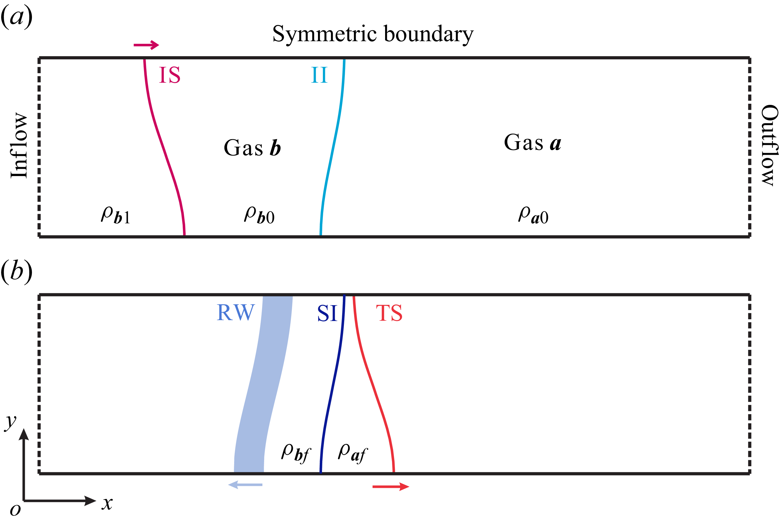
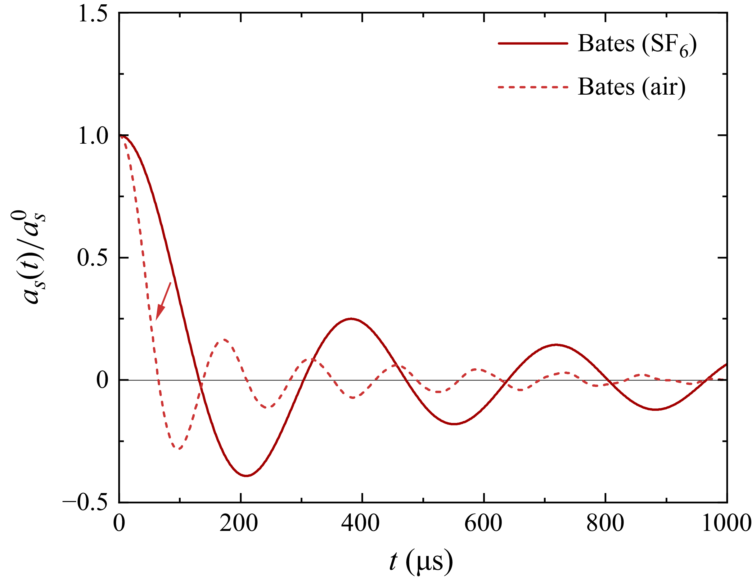
 6

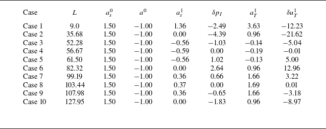
 as1
 δpI
 aT1
 δuT1
 ms−1
 104
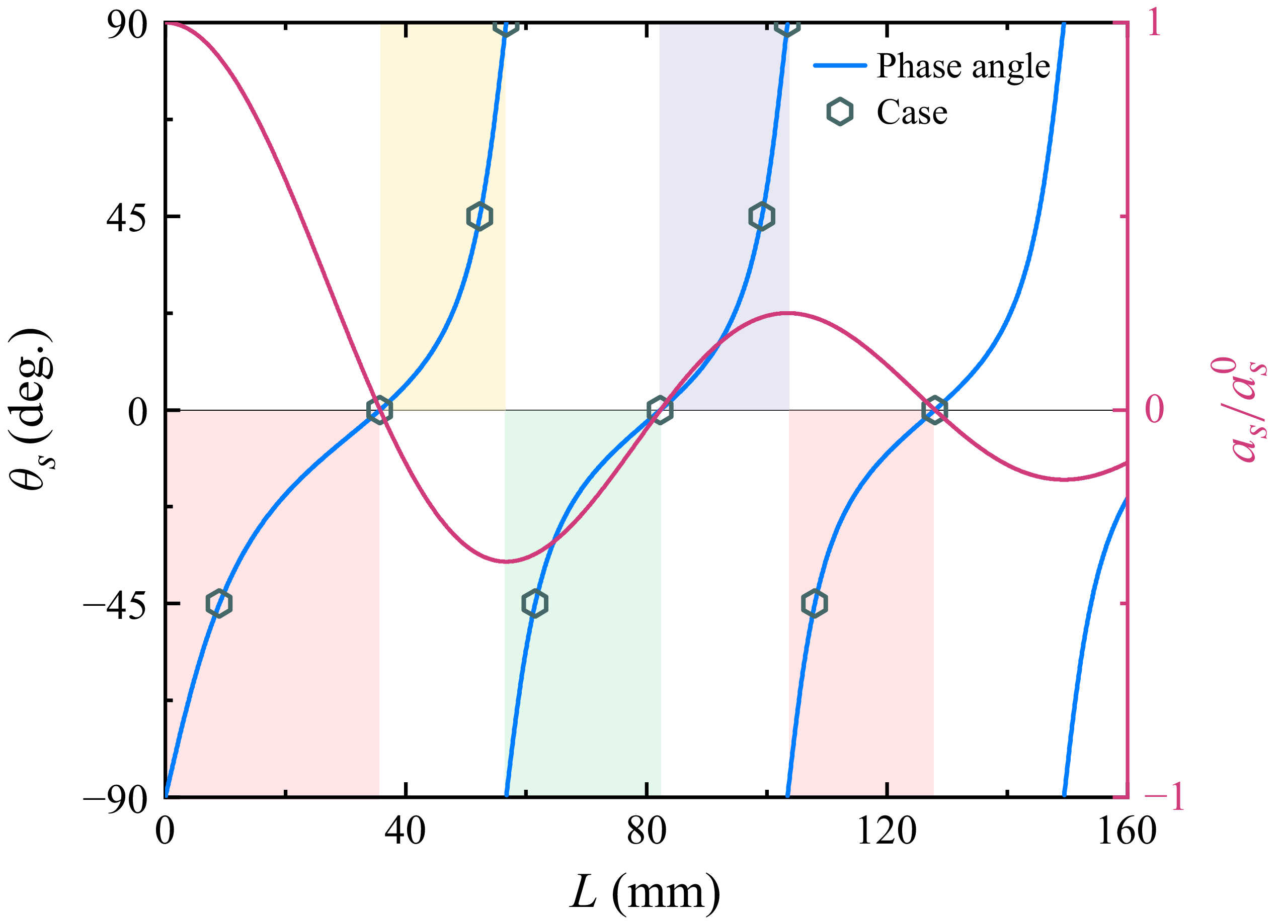
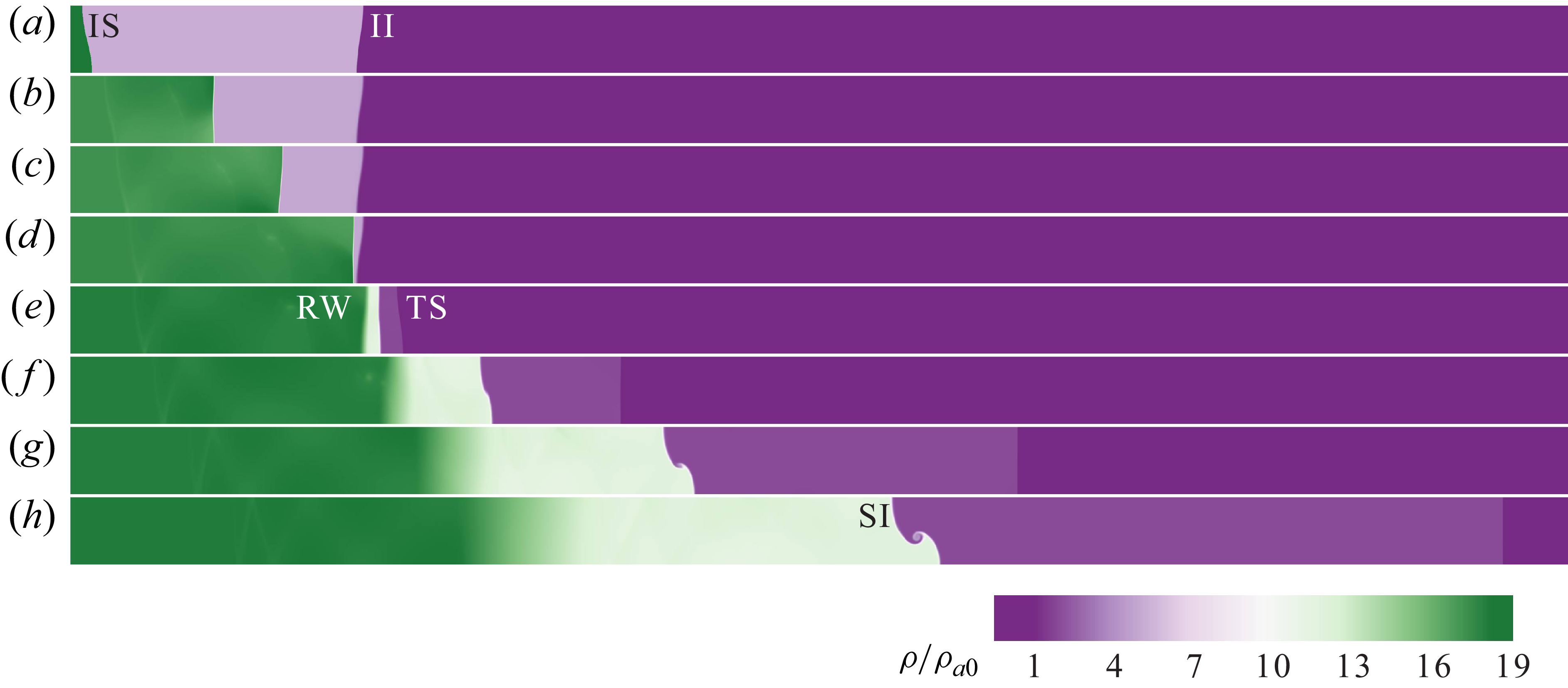


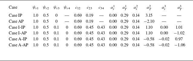
 1
 2
 3
 6
 ψv1
 ψv2
 ψv3
 ψv4
 6
 c12
 c23
 c34
 1
 2
 3
 as1
 aT1
 as2
 aT2
 as3
 aT3


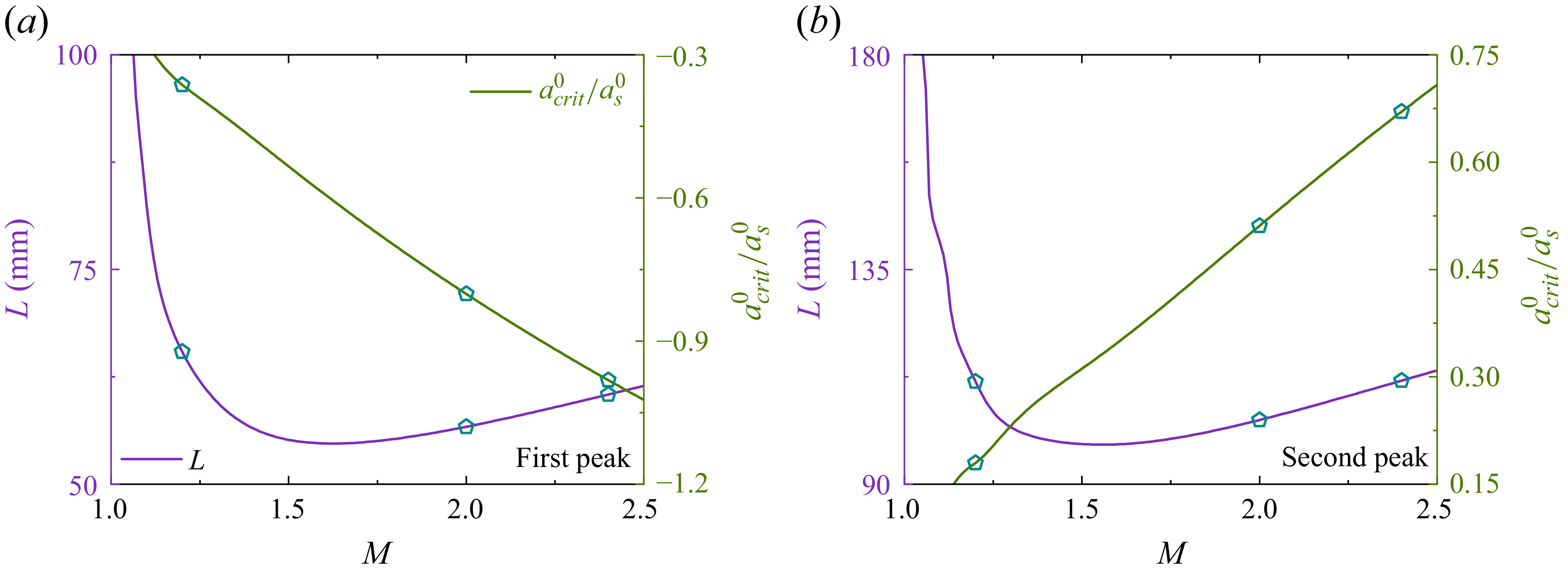

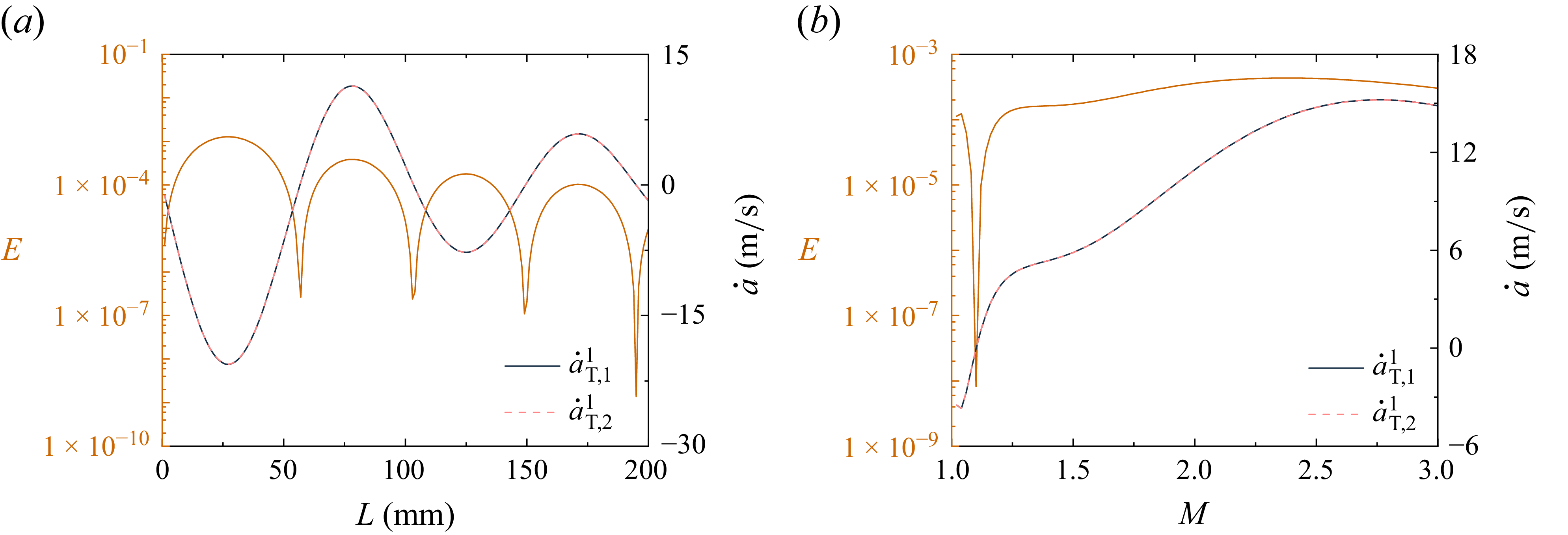
 L
 M=2.0
 M
 L=82.32 mm


