Robust flow control and optimal sensor placement using deep reinforcement learning

Romain Paris; Samir Beneddine; Julien Dandois

doi:10.1017/jfm.2020.1170

Robust flow control and optimal sensor placement using deep reinforcement learning

Published online by Cambridge University Press: 26 February 2021

and

Romain Paris*: Affiliation:
DAAA, ONERA, Université Paris Saclay, 92190 Meudon, France
Samir Beneddine: Affiliation:
DAAA, ONERA, Université Paris Saclay, 92190 Meudon, France
Julien Dandois: Affiliation:
DAAA, ONERA, Université Paris Saclay, 92190 Meudon, France
*: †Email address for correspondence: romain.paris@onera.fr

Article contents

Abstract
Introduction
Description of the flow configuration and numerical methods
Reinforcement learning algorithms
Results and discussion
Conclusion
References

Rights & Permissions

Abstract

This paper focuses on finding a closed-loop strategy to reduce the drag of a cylinder in laminar flow conditions. Deep reinforcement learning algorithms have been implemented to discover efficient control schemes, using two synthetic jets located on the cylinder's poles as actuators and pressure sensors in the wake of the cylinder as feedback observation. The present work focuses on the efficiency and robustness of the identified control strategy and introduces a novel algorithm (S-PPO-CMA) to optimise the sensor layout. An energy-efficient control strategy reducing drag by $18.4\,\%$ at a Reynolds number of $120$ is obtained. This control policy is shown to be robust both to a Reynolds-number variation in the range $[100;216]$ and to measurement noise, for signal-to-noise ratios as low as $0.2$ with negligible impact on performance. Along with a systematic study on sensor number and location, the proposed sparsity-seeking algorithm has achieved a successful optimisation to a reduced five-sensor layout while keeping state-of-the-art performance. These results further highlight the interesting possibilities of reinforcement learning for active flow control and pave the way to efficient, robust and practical implementations of these control techniques in experimental or industrial systems.

JFM classification

Flow Control: Drag reduction Flow Control: Instability control Vortex Flows: Vortex shedding

Information

Type: JFM Papers
Information: Journal of Fluid Mechanics , Volume 913 , 25 April 2021, A25
DOI: https://doi.org/10.1017/jfm.2020.1170 [Opens in a new window]
Copyright: © The Author(s), 2021. Published by Cambridge University Press

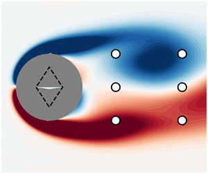
1. Introduction

Improvement of aerodynamic characteristics on aerial vehicles has mainly been achieved through shape optimisation in the past decades, with drag reduction as the primary goal. Passive control devices have long been the centrepiece of flow control (Selby, Lin & Howard Reference Selby, Lin and Howard1992; Gutmark & Grinstein Reference Gutmark and Grinstein1999; Marquet, Sipp & Jacquin Reference Marquet, Sipp and Jacquin2008) due to their ease of use. Yet, their overall low efficiency advocates for active forms of control, which are split into two categories: open-loop strategies (see e.g. Protas & Wesfreid Reference Protas and Wesfreid2002; Bergmann, Cordier & Brancher Reference Bergmann, Cordier and Brancher2005; Sipp Reference Sipp2012) may achieve interesting results but often at a high energetic cost; whereas closed-loop approaches (Sipp & Schmid Reference Sipp and Schmid2016) are known to display greater energy efficiency and robustness, taking advantage of state measurements. In this context, linear techniques have recently been investigated for active flow control.

These linear approaches often rely on a reduced-order model, mainly via proper orthogonal decomposition (POD) (Gerhard et al. Reference Gerhard, Pastoor, King, Noack, Dillmann, Morzynski and Tadmor2003; Bergmann et al. Reference Bergmann, Cordier and Brancher2005; Bergmann & Cordier Reference Bergmann and Cordier2008), which provides frameworks to apply linear open- and closed-loop control techniques. The cylinder wake flow has often been studied as a test case for the numerous approaches proposed in the literature. Fujisawa, Kawaji & Ikemoto (Reference Fujisawa, Kawaji and Ikemoto2001) and Siegel, Cohen & McLaughlin (Reference Siegel, Cohen and McLaughlin2003) used variable phase and proportional and differential control to reduce the drag of low-Reynolds-number cylinder flows. Atam, Mathelin & Cordier (Reference Atam, Mathelin and Cordier2016) used ARMAX/ARX models with gain scheduling to reach a target drag value in varying-Reynolds-number conditions. Several studies implemented robust $H_2$ or $H_\infty$ control methods based on resolvent analysis (Jin, Illingworth & Sandberg Reference Jin, Illingworth and Sandberg2019). Other mathematical frameworks, such as the adjoint approach (He et al. Reference He, Glowinski, Metcalfe, Nordlander and Periaux2000), have also shown efficient control but at a high computational cost. These are a few examples – all studying a two-dimensional (2-D) flow past a cylinder – of a large body of work relying on local linear approximations of the uncontrolled system. Such control strategies, often involving constant or periodic forcing on the flow, are successful for dynamical systems moderately modified by a small control actuation. In those cases, the linear approach remains valid.

However, the linear assumption is not satisfied in numerous practical fluid mechanics applications, when nonlinearities are strong and when control may significantly alter the dynamics. Energy-efficient states of the controlled system are sometimes poorly described by the linear approximations. Therefore, these states are often out of reach for linear strategies. This issue is highlighted in the work of Jin et al. (Reference Jin, Illingworth and Sandberg2019), who manage to stabilise the wake of a 2-D cylinder flow using body forces and a resolvent-based analysis but only up to Reynolds number $Re=100$. Their optimal linear control fails for higher values. Similarly, Leclercq et al. (Reference Leclercq, Demourant, Poussot-Vassal and Sipp2019) showed on a cavity flow that a linear approach based on modern control methods such as structured $H_\infty$ synthesis coupled with resolvent analysis was unable to suppress flow oscillations. To overcome this, they proceeded by iterative linearisations to update their control law, in a way reminiscent of Newton's method, where a nonlinear solution is found by solving successive linear problems. Unfortunately, such resolvent-based approaches may be computationally challenging for high-dimensional systems, and their robustness is unknown. Therefore, new robust and efficient nonlinear methods for flow control are still wanting.

In the context of the development of machine learning (ML) techniques, efficient nonlinear active flow control seems more and more feasible, as emphasised by Brunton & Noack (Reference Brunton and Noack2015) and Brunton, Noack & Koumoutsakos (Reference Brunton, Noack and Koumoutsakos2020). The use of artificial neural networks as universal function approximators that can be trained efficiently has already proven significant capabilities for solving complex problems, such as language translation (Cho et al. Reference Cho, Van Merriënboer, Gulcehre, Bahdanau, Bougares, Schwenk and Bengio2014; Sutskever, Vinyals & Le Reference Sutskever, Vinyals and Le2014) or image recognition (He et al. Reference He, Zhang, Ren and Sun2016). Coupled with reinforcement methods, which use interactions with the controlled environment to improve performance, these techniques achieve autonomous learning of complex tasks (Baker et al. Reference Baker, Kanitscheider, Markov, Wu, Powell, McGrew and Mordatch2019; Kaiser et al. Reference Kaiser, Babaeizadeh, Milos, Osinski, Campbell, Czechowski, Erhan, Finn, Kozakowski and Levine2019), and often perform better than human experts (Mnih et al. Reference Mnih, Kavukcuoglu, Silver, Rusu, Veness, Bellemare, Graves, Riedmiller, Fidjeland and Ostrovski2015). The present study focuses particularly on on-policy deep reinforcement learning (DRL). From the first methods (Williams Reference Williams1992) to the most recent algorithms, such as trust region policy optimisation (Schulman et al. Reference Schulman, Levine, Abbeel, Jordan and Moritz2015a) or proximal policy optimisation (PPO) and its variants (Schulman et al. Reference Schulman, Wolski, Dhariwal, Radford and Klimov2017; Hämäläinen et al. Reference Hämäläinen, Babadi, Ma and Lehtinen2020), DRL has demonstrated the ability to efficiently learn non-trivial control strategies (named policies) in complex and high-dimensional environments. By leveraging stochastic estimation and Markov processes, these algorithms optimise both sample and policy efficiencies.

The use of ML techniques in fluid mechanics enables efficient and more straightforward nonlinear control strategies, which could combine performance, energy efficiency and robustness. In the wake of nonlinear autoregressive models (Kim et al. Reference Kim, Kerr, Beskok and Jayasuriya2006; Dandois, Garnier & Pamart Reference Dandois, Garnier and Pamart2013), ML algorithms have been used either for black-box or model-based feedback control (Seidel et al. Reference Seidel, Siegel, Fagley, Cohen and McLaughlin2009; Cohen et al. Reference Cohen, Siegel, Seidel, Aradag and McLaughlin2012). Nørgård et al. (Reference Nørgård, Ravn, Poulsen and Hansen2000) also leveraged the flexibility of neural network structures using the artificial neural network estimator (ANNE) method. Semi-supervised learning methods, such as model predictive control (Nair et al. Reference Nair, Taira, Brunton and Brunton2020) or DRL for control (Rabault et al. Reference Rabault, Kuchta, Jensen, Réglade and Cerardi2019), also meet increasing success. Some relevant applications of DRL include the work of Colabrese et al. (Reference Colabrese, Gustavsson, Celani and Biferale2017), who trained swimmers in a non-uniform flow, or Bucci et al. (Reference Bucci, Semeraro, Allauzen, Wisniewski, Cordier and Mathelin2019), who successfully steered a one-dimensional chaotic system driven by the Kuramoto–Sivashinsky equation towards its fixed points with this technique. A drastic reduction of the heat flux through a Rayleigh–Bénard convection cell was performed by Beintema et al. (Reference Beintema, Corbetta, Biferale and Toschi2020). Belus et al. (Reference Belus, Rabault, Viquerat, Che, Hachem and Reglade2019) leveraged spatial invariance to replicate identical DRL-learned sensor–actuator systems along a one-dimensional liquid film to control its instability. These simple yet nonlinear test cases serve as proof of concept and illustrate the promising potential of DRL for real-world flow control cases. This potential has recently been confirmed by Shimomura et al. (Reference Shimomura, Sekimoto, Oyama, Fujii and Nishida2020), who used a plasma actuator driven by a DRL-learned policy to delay airfoil flow separation at a chord Reynolds number of $6.3\times 10^4$.

However, the known lack of extrapolation capabilities of neural networks in supervised learning applications points to the robustness of DRL methods as a potential weak point. This issue has been explored by Tang et al. (Reference Tang, Rabault, Kuhnle, Wang and Wang2020) and Ren, Rabault & Tang (Reference Ren, Rabault and Tang2020), who successfully controlled a 2-D cylinder wake across a large range of Reynolds numbers. These applications show the relevance of complex control over linear-approximation-based control for this kind of nonlinear system. In this present study, the potentialities of DRL in active flow control performance, power efficiency and robustness are investigated on a similar test case. One contribution of the paper relates to the introduction of a variant of PPO that is shown to outperform state-of-the-art DRL approaches on the cylinder case.

Another important contribution concerns optimal sensor placement. Reducing sensor requirements while keeping optimal control performances is crucial to potentially transpose these techniques to experimental and industrial cases in the future. Rabault et al. (Reference Rabault, Kuchta, Jensen, Réglade and Cerardi2019) and Tang et al. (Reference Tang, Rabault, Kuhnle, Wang and Wang2020), respectively, use 151 and 236 probes to control the flow past a 2-D cylinder. Their work is therefore a first step for DRL control, which needs to be continued and further improved, which is precisely the purpose of this work. The present study builds on these existing papers to propose new techniques and algorithms that reduce the gap between DRL capabilities for flow control and the requirements for a future experimental or industrial implementation. Having fewer sensors means, at the same time, less hardware requirements, fewer potential failure modes and less computational power needs, especially in the context of embedded systems with strong real-time computing constraints.

This issue of optimal measurement location has been investigated by many authors outside of the context of DRL, for instance by Foures et al. (Reference Foures, Dovetta, Sipp and Schmid2014), Mons et al. (Reference Mons, Chassaing, Gomez and Sagaut2016), Mons, Chassaing & Sagaut (Reference Mons, Chassaing and Sagaut2017) and Verma et al. (Reference Verma, Papadimitriou, Lüthen, Arampatzis and Koumoutsakos2020) for data assimilation. Bright, Lin & Kutz (Reference Bright, Lin and Kutz2013) took advantage of compressed sensing to perform flow reconstruction using a limited number of sensors. The optimal estimation of a reduced-order state, usually POD modes, has been used by Cohen, Siegel & McLaughlin (Reference Cohen, Siegel and McLaughlin2006) and Seidel et al. (Reference Seidel, Siegel, Fagley, Cohen and McLaughlin2009), and echoes the assumption that accurate flow estimation is an essential feature of efficient control. However, as stressed by Oehler & Illingworth (Reference Oehler and Illingworth2018), control does not systematically require faithful flow reconstruction (in the sense of POD); the partial knowledge of relevant ‘hidden’ variables may be sufficient. This idea is conveyed by the notion of observability Gramian, in the linear framework. Empirical observability Gramians were used by Singh & Hahn (Reference Singh and Hahn2005) and DeVries & Paley (Reference DeVries and Paley2013) for flow estimation, and a version balancing both observability and controllability Gramians was successfully implemented by Manohar, Kutz & Brunton (Reference Manohar, Kutz and Brunton2018) to design an optimal $H_2$ control of a linearised Ginzburg–Landau model. One of the main contributions of our work is to propose a new method, leveraging a previously learned DRL policy to optimise sensor location.

In the following, the simulated case study is first introduced, then the DRL algorithm used to derive the control strategy is described and a new sparsity-seeking variant of this algorithm, aiming at optimising sensor number and location, is proposed. The main results and discussions are developed in § 4. The issue of control efficiency and robustness to both Reynolds-number variations and measurement noise is addressed in this section. Finally, the optimised sensor layouts derived using our proposed method are discussed.

2. Description of the flow configuration and numerical methods

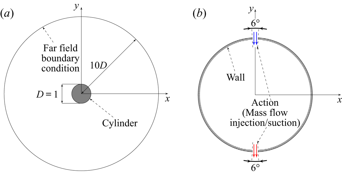
The studied configuration is a 2-D flow past a cylinder. The geometry is made non-dimensional by setting the cylinder diameter $D$ to 1. The centre of the cylinder is located at the origin $(0,0)$ of the flow domain. Figure 1 displays the computed flow domain, which spans over $10D$, and shows the orientation of axes $x$ and $y$.

Figure 1.

Flow domain geometry. (a) Full domain, not at true scale. The far field boundary condition is a characteristic-based inflow/outflow boundary condition modelling free-stream flow. (b) Boundary conditions on the cylinder.

2.1. Numerical set-up

The flow is described by the compressible Navier–Stokes (NS) equations. The free-stream flow is uniform at a Mach number $M_\infty$ of $0.10$, oriented along $x$. In the following, all quantities are made non-dimensional by the characteristic length $D$, the inflow density $\rho _\infty$, the velocity $U_\infty$ and the static temperature $T_\infty$. Note that the Mach number is very low, such that the density fluctuations in the whole domain are negligible, and the flow is therefore quasi-incompressible. 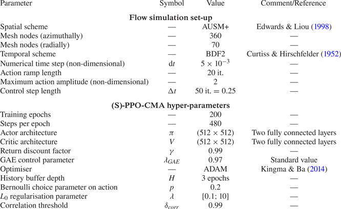The Reynolds number $Re$, defined as $U_\infty D/\nu$ ($\nu$ being the kinematic viscosity), is varied in the article, but the first sections of the paper focus on a reference configuration at $Re=120$. The flow field is computed via direct numerical simulation using ONERA's FastS finite-volume method solver (Dandois, Mary & Brion Reference Dandois, Mary and Brion2018) for both steady and unsteady computations. The spatial discretisation is based on the second-order-accurate AUSM+(P) scheme described by Edwards & Liou (Reference Edwards and Liou1998), and the time integration of the equations is performed with a second-order implicit Euler scheme. For unsteady computations, a global numerical time step $\textrm {d}t=5\times 10^{-3}$ is chosen. Steady solutions are converged using a local time-stepping strategy. Additional numerical details are available in Appendix D. The C-shaped structured mesh is made of 25 200 nodes and is refined in the vicinity of the cylinder. The boundary conditions are specified in figure 1.

As shown in figure 1, injection or suction is performed on the cylinder's poles through two $6^\circ$-wide jet inlets. The control step $\Delta t$ is defined as the number of numerical iterations during which the control command is held constant. In this study, a control step lasts for $50$ numerical time steps, and thus $\Delta t=0.25$ non-dimensional time units. As discussed by Rabault & Kuhnle (Reference Rabault and Kuhnle2019), this control step choice is driven by both flow and controller time horizons. The natural vortex shedding period imposes a higher bound on the control step for both measurement and action to identify the dynamics without aliasing. Fifty numerical steps correspond to approximately 22 control actions per vortex shedding period. As described in § 3, the controller imposes a lower-bound constraint since the impact of a given action $a_t$ should not be sensed in a ‘too-distant’ future, that is within a reasonable number (${<}100$) of control steps later. For each control step, a command $a_t$ (positive or negative) is translated into a blowing/suction using a 20-iteration interpolation ramp which avoids abrupt changes of boundary conditions and non-physical values due to the numerical schemes (similarly to what Rabault et al. (Reference Rabault, Kuchta, Jensen, Réglade and Cerardi2019) did). Formally, for the $i$th numerical iteration of the control step, the mass flow per unit area $q_i$ is

(2.1)

\begin{equation} q_i = \rho_\infty U_\infty (a_{t-1}(1-r_i) + a_tr_i ), \quad \text{with } r_i = \left\{\begin{matrix} i/20 , & \text{ if } i<20,\\ 1, & \text{ otherwise}, \end{matrix}\right. \end{equation}

while the stagnation enthalpy is held constant in the case of blowing. To ensure an instantaneous zero-net-mass flux for every action, the two poles act reciprocally: $+q_i$ is imposed on the top inlet surface and $-q_i$ on the bottom inlet. Note that, in several studies, the actuators are such that they are able to inject streamwise momentum, which may directly reduce the cylinder drag. In the present study, the actuators are designed such that they can only inject cross-stream momentum, thus making any ‘direct’ drag reduction impossible.

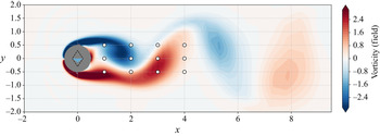
Several sensors record the pressure of the flow at predefined locations and at the end of every control step. The standard grid-like sensor layout is made of 12 sensors at locations $(x,y)\in \{1,2,3,4\}\times \{-0.5,0,0.5\}$. The output measurement is a pressure fluctuation, defined as the difference between the local non-dimensional static pressure and the reference inflow static pressure $p_\infty$. Figure 2 illustrates a standard set-up for this case.

Figure 2.

Instantaneous vorticity flow field with action $a_t=-0.15$ at $Re=120$. White circles represent the sensor locations. The coloured triangle in the cylinder depicts the action, its height and colour representing its amplitude. The dashed diamond shape marks off maximum actions (both positive and negative).

Both drag and lift coefficients ($C_x$ and $C_l$) are computed on the cylinder via the resulting force of the flow $\boldsymbol {F}$:

(2.2)

\begin{gather} \boldsymbol{F} = \int_{{cylinder}}\boldsymbol{\sigma}\boldsymbol{\cdot}{\boldsymbol{n}}\,\textrm{d}S, \end{gather}

(2.3)

\begin{gather} C_x = \frac{\boldsymbol{F}\boldsymbol{\cdot}\boldsymbol{e}_x}{\frac{1}{2}\rho_\infty U_\infty^2 D}, \end{gather}

(2.4)

\begin{gather} C_l = \frac{\boldsymbol{F}\boldsymbol{\cdot}\boldsymbol{e}_y}{\frac{1}{2}\rho_\infty U_\infty^2 D}, \end{gather}

where $\boldsymbol {n}$ is the unitary cylinder surface normal vector, $\boldsymbol {\sigma }$ is the stress tensor, $\boldsymbol {e}_x = (1,0)$ and $\boldsymbol {e}_y = (0,1)$.

2.2. Uncontrolled flow

The uncontrolled configuration, denoted in the following as the baseline flow, displays a well-documented vortex shedding behaviour (Williamson Reference Williamson1996) that appears for Reynolds numbers above 46 and which is due to a Hopf bifurcation where the steady solution of the NS equations (the base flow) becomes unstable. Thus, the flow becomes unsteady and follows a stable limit cycle associated with vortex shedding.

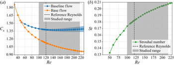
As presented in figure 3, values of the drag coefficient and Strouhal number (defined as $St = fD/U_\infty$, with $f$ being the vortex shedding frequency) have been computed for a wide range of Reynolds numbers to ensure consistency with other studies (Nishioka & Sato Reference Nishioka and Sato1978; Braza, Chassaing & Minh Reference Braza, Chassaing and Minh1986; Williamson Reference Williamson1996; Henderson Reference Henderson1997; He et al. Reference He, Glowinski, Metcalfe, Nordlander and Periaux2000; Bergmann et al. Reference Bergmann, Cordier and Brancher2005). For $Re=120$, the drag coefficient is $1.379$ with fluctuations of amplitude $0.018$, and $St = 0.18$, which is in agreement with the literature (Barkley Reference Barkley2006; Sipp et al. Reference Sipp, Marquet, Meliga and Barbagallo2010). Note that, since the simulation solves the 2-D NS equations, the flow remains laminar across the studied Reynolds-number range and does not undergo any additional stability bifurcation.

Figure 3.

(a) Evolution of the time-averaged drag coefficient of the baseline flow (blue) and the base flow (orange) with the Reynolds number. The blue shaded area indicates the variation range of the drag coefficient $C_x$. (b) Evolution of the Strouhal number of the vortex shedding with the Reynolds number.

Following the work of Protas & Wesfreid (Reference Protas and Wesfreid2002), the total drag $C_{x,0}$ of the baseline flow can be decomposed into two contributions: the drag of the base flow $C_{x,BF}$, which is constant; and the drag correction due to the flow unsteadiness $C_{x,U}$. If $\langle \,{\cdot }\,\rangle _{T}$ denotes the time average over a vortex shedding period $T$, then

(2.5)

\begin{equation} \langle C_{x,0} \rangle_T = C_{x,BF} + \langle C_{x,U} \rangle_T. \end{equation}

Using the base-flow performance as a reference, let us define the drag gain $\mu _{C_x}$ as a fraction of the drag reduction achieved by the base flow:

(2.6)

\begin{equation} \mu_{C_x} = \frac{\langle C_{x,0} \rangle_T-C_x}{\langle C_{x,U}\rangle_T}. \end{equation}

This quantity measures the relative drag reduction due to the control. Thus, a drag gain $\mu _{C_x}$ of 100 % is equivalent to a complete suppression of the vortex shedding. Protas & Wesfreid (Reference Protas and Wesfreid2002) also asked whether a negative mean drag correction $\langle C_x-C_{x,BF}\rangle _T$ could be reached with a periodic forcing, implying a drag gain larger than $100\,\%$. Examples from the literature, such as the work of He et al. (Reference He, Glowinski, Metcalfe, Nordlander and Periaux2000) and Tang et al. (Reference Tang, Rabault, Kuhnle, Wang and Wang2020), who achieved $\mu _{C_x}=108\,\%$ and $\mu _{C_x}=105\,\%$ at $Re=200$, respectively, show that this is possible. However, in the case of He et al. (Reference He, Glowinski, Metcalfe, Nordlander and Periaux2000), this performance comes at the cost of a significantly modified mean flow and a large actuation. As shown later, the present study also achieves drag gains slightly higher than 100 %, while both preserving the base-flow structure and being energy-efficient.

3. Reinforcement learning algorithms

3.1. A short description of ‘on-policy reinforcement learning’

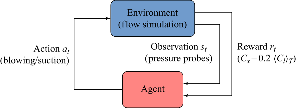
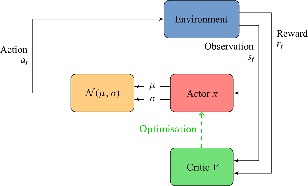
Reinforcement learning considers an environment in interaction with an agent as illustrated in figure 4. At each control step $t$, the agent receives partial state observations $s_t$ and a reward $r_t$ quantifying the current performance of the environment. The agent then takes an action $a_t$ based on the observations, through a policy $\pi$: $a_t\sim \pi (\cdot ,s_t)$. This policy can be either deterministic or stochastic. The objective of the training is to derive a policy $\pi ^*$ that maximises the cumulative reward (called return) throughout time.

Figure 4.

Reinforcement learning feedback loop.

In the present study, the environment is the previously described numerical case and the goal is to minimise drag. Thus the reward is a defined as

(3.1)

\begin{equation} r_t ={-} C_x - \alpha | \langle C_l \rangle_T | , \end{equation}

with $\langle C_l \rangle _T$ being a moving average of the lift coefficient on the previous 22 control steps corresponding to the duration of a vortex shedding period, and $\alpha$ the corresponding regularisation coefficient. Here $\alpha =0.2$ (this value is discussed in § 4.1). This penalisation ensures a nearly ‘zero time-averaged lift’ policy. Pressure sensors provide the observed information; actions are computed within a valid range ($a_t\in [-2;2]$) and then implemented on the environment as previously described. Note that the optimised actions of the trained policy do not reach the prescribed bounds. Therefore, choosing higher values for the valid range of $a_t$ does not affect the final results (but it may lead the solver to crash during training if too high values are allowed). The code architecture relies on the Tensorflow software library (Abadi et al. Reference Abadi, Barham, Chen, Chen, Davis, Dean, Devin, Ghemawat, Irving and Isard2016) and is interfaced with the simulation environment through the Cassiopée application programming interface (Benoit, Péron & Landier Reference Benoit, Péron and Landier2015) using the Python programming language. Interface standards are inspired from Open AI's Gym toolkit (Brockman et al. Reference Brockman, Cheung, Pettersson, Schneider, Schulman, Tang and Zaremba2016).

All learning algorithms aim at solving the exploration–exploitation dilemma, meaning achieving the best performance at a minimum learning cost. Efficient exploration of the state–action subspace is a key factor in the performance of the learning algorithm. The exploration is performed through the introduction of randomness in actions. However, too much randomness deteriorates the learning speed and thus reduces exploitation performances for a given learning budget. The careful control of the exploration variance is thus crucial. On-policy algorithms try to circumvent this issue using the most recent (and best so far) version of the policy to collect experience, thus sparing inefficient exploration in suboptimal regions of the state–action subspace.

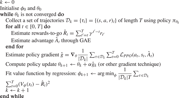
One of the state-of-the-art learning approaches is the PPO introduced by Schulman et al. (Reference Schulman, Wolski, Dhariwal, Radford and Klimov2017). PPO displays better sample efficiency compared to other DRL methods. It can be used for high-dimensional, continuous state spaces and has been successfully implemented by Rabault et al. (Reference Rabault, Kuchta, Jensen, Réglade and Cerardi2019, Reference Rabault, Ren, Zhang, Tang and Xu2020) and Rabault & Kuhnle (Reference Rabault and Kuhnle2019) on a very similar case study. This on-policy actor–critic algorithm uses a dual neural network structure, an ‘actor’ ($\pi$) and a ‘critic’ ($V$), as agent. Both networks are fed with the observations $s_t$. The actor outputs an optimal action $\mu _t=\mu _\theta (s_t)$, $\theta$ being the weights and biases of $\pi$. Then, using a predefined standard deviation $\sigma$, an action $a_t\sim \pi _\theta (\cdot |s_t) = \mathcal {N}(\cdot |\mu _\theta ,\sigma )$ is sampled, $\mathcal {N}$ being a normal distribution. The critic outputs an estimate of the value $V_t=V_\phi (s_t)$ of the observed state $s_t$, $\phi$ being the weights and biases of $V$. This value is an estimator of the expected return $R_t = \sum _{\tau =t}^{\infty } \gamma ^\tau r_\tau$, with $\gamma \in \,]0;1[$ being a discount factor. The value $V_t$ is used during the update of $\pi _\theta$ to improve learning. The learning phase is performed using a surrogate objective: the updated weights $\theta _{new}$ of the actor aim at making the most successful actions more likely, using the probability ratio ${\pi _{\theta _{new}}(a_t,\mu _t,\sigma )}/{\pi _{\theta }(a_t,\mu _t,\sigma )}$. However, to prevent excessively large policy updates, the surrogate objective is clipped. As a consequence, the exploration variance, which is due to both $\sigma$ and the variability of $\mu _t$, often shrinks prematurely as explained by Hämäläinen et al. (Reference Hämäläinen, Babadi, Ma and Lehtinen2020). The next section presents a variant of the PPO algorithm, used in this paper, which addresses this limitation. Refer to Appendix C for more detail on PPO.

3.2. Standard proximal policy optimisation with covariance matrix adaptation

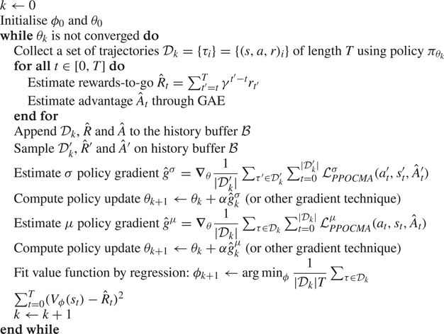
Proximal policy optimisation with covariance matrix adaptation (PPO-CMA) (Hämäläinen et al. Reference Hämäläinen, Babadi, Ma and Lehtinen2020) is a variant of PPO that prevents the premature vanishing of the exploration variance using the covariance matrix adaptation technique introduced by the CMA-ES evolutionary algorithm (Hansen, Müller & Koumoutsakos Reference Hansen, Müller and Koumoutsakos2003; Hansen Reference Hansen2016). Unlike PPO, the covariance matrix $\sigma$ used to sample the action $a_t\sim \mathcal {N}(\cdot ,\mu ,\sigma )$, is an output of the actor $\pi$, as shown in figure 5, and the surrogate objective used for updates is not clipped. A more detailed description of PPO-CMA is provided in Appendix C. PPO-CMA is used for all the results introduced in §§ 4.1–4.4. As shown in the following and for the same number of trainable parameters, it yields significantly improved performances than the ‘vanilla’ PPO algorithm used by Rabault et al. (Reference Rabault, Kuchta, Jensen, Réglade and Cerardi2019). Their study shows that a structure made of two fully connected layers of 512 neurons for both ‘actor’ and ‘critic’ networks was sufficient to encode their control law. Several layer sizes, ranging from 64 to 1024 neurons, have been tested in the present study and they all yield similar results. For the sake of comparison, the same set-up using $2\times 512$ neurons is used in the following.

Figure 5.

PPO-CMA. The actor $\pi$ receives observations $s_t$ from the environment and outputs $\mu$ and $\sigma$, which are used to sample action $a_t$. The critic $V$ estimates the value $V_t$ of the observed state $s_t$. During the update phase, $V_t$ is used to update the actor and the critic is updated using supervised learning on the effective state values $R_t=\sum _{\tau =t}^{\infty }\gamma ^\tau r_\tau$ (observed returns).

3.3. Sparse surrogate actor

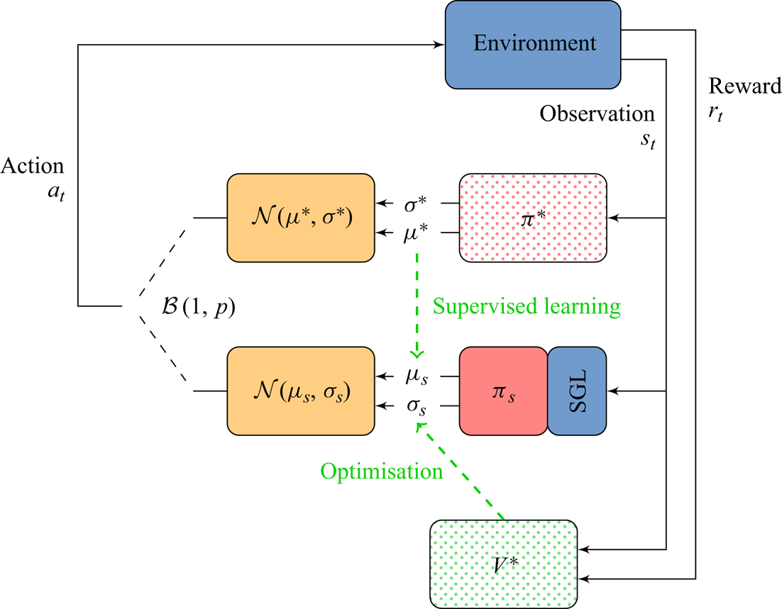
A novel algorithm called sparse proximal policy optimisation with covariance matrix adaptation (S-PPO-CMA), selecting relevant observations and discarding non-necessary or redundant sensor information, while preserving the optimality of the learned control strategy as much as possible, is introduced. Note that S-PPO-CMA is only used in § 4.5 to optimise the number and location of sensors, the other results presented in this study being obtained with standard PPO-CMA. This method splits into two separate phases: training a conventional PPO-CMA actor–critic structure (described in § 3.2), then deriving a sparse surrogate actor. The sparse training phase relies on the previously trained PPO-CMA actor–critic policy denoted by $\pi ^*$ for the actor and $V^*$ for the critic. As described by figure 6, the sparse actor $\pi _s$ is composed of a dense neural network having the same structure (architecture and activation functions) as $\pi ^*$, to which a stochastic gated input layer (SGL) is added.

Figure 6.

S-PPO-CMA. Actions are sampled using either the reference actor $\pi ^*$ or the sparse actor $\pi _s$ via a Bernoulli choice $\mathcal {B}(1,p)$. Then $\pi _s$ is updated via learning on $\sigma _s$ using values from $V^*$ and by supervised learning on $\mu _s$ using $\mu ^*$ values. The parameters of the SGL are also updated during this phase.

During the sparse training phase, the action $a_t$ is sampled using either the optimal policy $\pi ^*$ or $\pi _s$, using a Bernoulli random variable. Both training of $\pi ^*$ and $V^*$ are stopped, but their outputs are used to train $\pi _s$ and the SGL that make up the sparse version of $\pi ^*$.

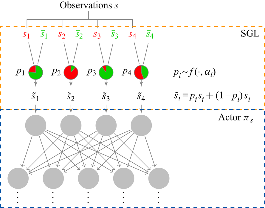
The SGL mechanism used here is inspired by the stochastic gate model proposed by Louizos, Welling & Kingma (Reference Louizos, Welling and Kingma2017). Let $n$ be the number of sensors (or the dimension of the observation space). The SGL, presented in figure 7, is a special simply connected layer that provides inputs to $\pi _s$ and that contains substitute values $\bar {\boldsymbol {s}}=(\bar {s}_1,\bar {s}_2,\ldots ,\bar {s}_n)$ for each observation component. Every time an observation vector $\boldsymbol {s}=(s_1,s_2,\ldots ,s_n)$ is received, the SGL samples a random vector $\boldsymbol {p}\in [0;1]^{n}$ that determines its output $\tilde {\boldsymbol {s}}$ such as

(3.2)

\begin{equation} \tilde{\boldsymbol{s}} = \boldsymbol{p}\odot\boldsymbol{s}+(1-\boldsymbol{p})\odot\bar{\boldsymbol{s}}, \end{equation}

where $\odot$ represents the element-wise product. Thus, $p_i=1$ outputs the observation $s_i$ whereas $p_i=0$ gives its substitute value $\bar {s}_i$, and any value in between provides a linear combination of $s_i$ and $\bar {s}_i$. Similarly to Louizos et al. (Reference Louizos, Welling and Kingma2017), $\boldsymbol {p}$ is sampled over a ‘gating’ distribution $f$:

(3.3)

\begin{gather} \boldsymbol{u}\sim \mathcal{U}^n(0,1), \end{gather}

(3.4)

\begin{gather} \boldsymbol{p}= f(\boldsymbol{u},\boldsymbol{\alpha}) = \text{clip}\left((\zeta-\gamma)\,\text{Sigmoid}\left[\frac{1}{\beta}(\log \boldsymbol{u} - \log (1-\boldsymbol{u})+\boldsymbol{\alpha})\right]+\gamma,\ 0,\ 1\right), \end{gather}

with $\mathcal {U}^n(0,1)$ denoting a uniform distribution on $[0,1]^n$, $\beta$, $\gamma$, $\zeta$ being fixed numerical parameters, $\boldsymbol {\alpha }$ being a trainable vector steering the expectation on $\boldsymbol {p}$ and $\text {clip}(a,b,c) = \min (\max (a,b),c)$. Here $f$ can be seen as a ‘soft’ Bernoulli choice distribution enabling values of $\boldsymbol {p}$ in $[0;1]^n$. The $L_0$ complexity of the SGL, giving the expected number of observation components $s_i$ for which $p_i>0$, can be written as

(3.5)

\begin{equation} \mathcal{L}_c (\boldsymbol{\alpha} ) = \sum_{i=1}^{n} P(p_i>0) = \sum_{i=1}^n \text{Sigmoid}\left[\alpha_i-\beta\log\frac{-\gamma}{\zeta}\right]. \end{equation}

During testing, $\boldsymbol {p}^*$, the most likely value of $\boldsymbol {p}$, is chosen deterministically as

(3.6)

\begin{equation} \boldsymbol{p}^*=\text{clip} ((\zeta-\gamma)\,\text{Sigmoid}[\boldsymbol{\alpha}]+\gamma,0,1 ). \end{equation}

Both $\boldsymbol {p}$ and $\boldsymbol {p}^*$ can take values between $0$ and $1$ (inclusive), thus modelling a fully ‘open’ or fully ‘closed’ gate while still allowing for a gradient-based optimisation using the loss $\mathcal {L}_c$.

Figure 7.

SGL. Received observation $s_i$ is either passed on to the actor $\pi _s$ if $p_i=1$, combined with its substitute value $\bar {s}_i$ if $p_i\in \,]0;1[$, or replaced by $\bar {s}_i$ if $p_i=0$. Here $p_i$ is sampled using a ‘gating’ function $f$ parametrised by $\alpha _i$, which is updated during the second phase of the S-PPO-CMA method.

3.4. Sparse actor training

The weights $\theta _s$ of the sparse actor $\pi _s$ are initialised using the weights $\theta ^*$ of $\pi ^*$ and updated every epoch by both the training of $\sigma _s$ and $\mu _s$. Also, $\sigma _s$ is trained in the same way $\sigma ^*$ has been trained (refer to Appendix C). Concerning $\mu _s$, however, a supervised learning using the optimal action $\mu ^*$ is performed with the loss

(3.7)

\begin{equation} \mathcal{L}_{ \pi_s} (\theta_s,\boldsymbol{\alpha} ) =\|\mu_s (\boldsymbol{s},\theta_s,\boldsymbol{\alpha} )-\mu^* (\boldsymbol{s},\theta^* )\|_1. \end{equation}

For the SGL, $\boldsymbol {\alpha }$ and $\bar {\boldsymbol {s}}$ are trained in the same process as $\theta _s$, allowing $\pi _s$ to ‘adapt’ to the variations of input $\tilde {\boldsymbol {s}}$ caused by the updates of the SGL. And $\bar {\boldsymbol {s}}$ is slowly updated using the observation values $\boldsymbol {s}$ at every epoch, and updates of $\boldsymbol {\alpha }$ are based on the following loss $\mathcal {L}_{{sparse}}$:

(3.8)

\begin{equation} \mathcal{L}_{{sparse}}=\mathcal{L}_{ \pi_s} (\theta_s,\boldsymbol{\alpha} ) +\lambda[\mathcal{H}_{1}(\mathcal{L}_c(\boldsymbol{\alpha}))+\boldsymbol{\varGamma}\boldsymbol{\alpha}], \end{equation}

where $\lambda$ is the regularisation parameter, $\mathcal {H}_1$ is a unitary Huber loss and $\boldsymbol {\varGamma }$ can be seen as a Tikhonov matrix that accounts for strong correlations between observations. Its purpose is to penalise $\alpha _i$ whose observation $s_i$ is correlated with any other $s_{j\neq i}$ and thus is redundant (refer to Appendix C for more details). The choice of $\lambda$ drives the equilibrium between sparsity and control performance.

4. Results and discussion

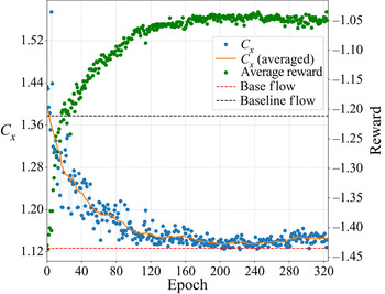
Unless otherwise stated, all results are obtained using the reference case at $Re=120$, with the 12-sensor layout described in figure 2 and PPO-CMA as learning algorithm. Figure 8 illustrates a standard learning process. A large variation of mean $C_x$ values can be observed in the first epochs of training; then $C_x$ values concentrate more around their moving average. This is caused by PPO-CMA decreasing the exploratory variance $\sigma$ when performance stabilises. For all the following results, training is performed sequentially (unlike in Rabault & Kuhnle (Reference Rabault and Kuhnle2019), who explored the potential of parallelised learning). A standard training of 200 epochs of 480 control steps each requires around 180 s per epoch on four CPU cores. Hence, a training of 200 epochs costs around 40 CPU hours, most of the CPU time being used to run the environment.

Figure 8.

Standard learning process. Each $C_x$ value is averaged over the whole epoch, including the transient from developed vortex shedding to controlled flow. This explains the discrepancy with pure performance values on $C_x$ later introduced. The orange curve is a 20-epoch moving average of $C_x$ values. The average reward (green dots, reward $r_t$ averaged over the current epoch) shows a quasi-monotonic growth that saturates from epoch $200$ onwards.

4.1. Control performance and efficiency

At a Reynolds number of 120, the time-averaged baseline flow drag coefficient is $\langle C_{x,0}\rangle = 1.379$. Performance in terms of drag reduction is computed as a percentage of the average baseline flow drag coefficient $\langle C_{x,0}\rangle$ and also using the drag gain $\mu _{C_x}$ introduced in § 2.2. 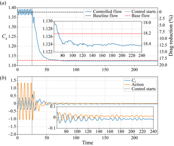Figure 9 shows the instantaneous drag coefficient $C_x$, the corresponding action $a_t$ and instantaneous lift coefficient $C_l$ throughout the control steps. A first phase, from time $t=25$ (control starting) to $t=50$ approximately, shows a rapid transient from the fully developed vortex shedding instability to the controlled flow. This transient corresponds to approximately $4.5$ vortex shedding periods. During that phase, actions have a large amplitude and do not seem to follow any simple pattern. In a second phase, from time $50$ to the end, the drag coefficient is stabilised to a value below $C_{x,BF}$. This represents a drag reduction of approximately $18.4\,\%$ and a drag gain $\mu _{C_x}$ around $100.6\,\%$. Actions have a significantly reduced amplitude compared to the first phase, and they appear to have a slightly non-zero average. Starting from $t=150$, a periodic action pattern seems to appear in the form of modulated bursts. These last two points are further discussed in § 4.2.

Figure 9.

Performance of the active flow control strategy. (a) Evolution of the instantaneous drag coefficient $C_x$. (b) Evolution of both action and lift coefficient $C_l$.

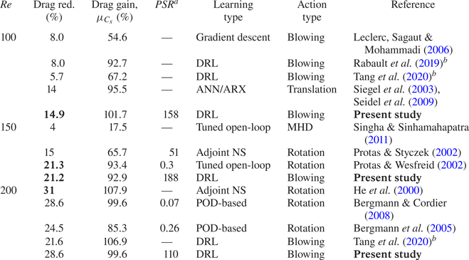
For other Reynolds-number values, drag reduction has also been measured. Results are presented in table 1 and confronted with other studies carried out on the same case.

(i) At $Re=100$, a drag gain slightly larger than $100\,\%$ is also reached. The observed mean flow is similar to the base flow.
(ii) At $Re=150$, the net drag reduction is more than $21\,\%$, close to the value reached by Protas & Wesfreid (Reference Protas and Wesfreid2002). In their case, they used large-amplitude rotary open-loop control, causing the controlled flow to remain unsteady. In the case of blowing/suction, a similar open-loop strategy has been tested at $Re=120$, with far less success in terms of drag reduction. This proves the limitations of open-loop strategies for the current blowing/suction set-up.
(iii) At $Re=200$, the results from He et al. (Reference He, Glowinski, Metcalfe, Nordlander and Periaux2000) slightly outperform those of the present study in terms of drag reduction. But their drag gain is also obtained at the cost of an important mean flow modification, as previously mentioned in § 2.2.

Table 1.

Drag reduction and performance comparison. Action types: ‘Blowing’, blowing/suction on cylinder poles; ‘Translation’, vertical translation of the cylinder; ‘MHD’, magnetohydrodynamic forcing; ‘Rotation’, rotation of the cylinder. Bold items are the best performances at each Reynolds number. $^{a\,}$Power-saving ratio. $^{b\,}$These cases are slightly different since walls parallel to the flow are added.

Some existing studies on the control of the cylinder flow have not been included in table 1 due to the significant discrepancies of their test case compared to ours, which prevents any straightforward comparison. For instance, Min & Choi (Reference Min and Choi1999), using a $360^\circ$ blowing/suction actuation, end up artificially reducing the equivalent diameter of their cylinder. While their results and methodology are interesting, comparison of performances is, however, not relevant here. Atam et al. (Reference Atam, Mathelin and Cordier2016) used a $360^\circ$ suction actuation steered by four different controllers and manage to match a target drag efficiently. The work of Arakeri & Shukla (Reference Arakeri and Shukla2013), who impose a tangential velocity on the cylinder surface and force a quasi-upstream–downstream symmetric flow, is not included in the comparison for similar reasons. Among the related – yet not directly comparable – interesting work, we can also cite Sohankar, Khodadadi & Rangraz (Reference Sohankar, Khodadadi and Rangraz2015), who achieve a significant drag reduction ($67\,\%$) for a porous square cylinder flow at $Re=100$, the paper from Muddada & Patnaik (Reference Muddada and Patnaik2010), which shows rather important gains (a drag reduction of $53\,\%$) using two small rotating rods in the vicinity of the cylinder, or the results from Chen & Aubry (Reference Chen and Aubry2005) using magnetohydrodynamic forcing to stabilise a cylinder flow at $Re=200$. For a more exhaustive list on the topic, one may refer to the review by Rashidi, Hayatdavoodi & Esfahani (Reference Rashidi, Hayatdavoodi and Esfahani2016).

Another important indicator of the control performance is the energy required for drag reduction. The instantaneous actuation power is computed as $P_{act}=\sum _{i=1}^2|q_i\Delta p_iS/\rho |\approx |a_t|S\rho _\infty U_\infty U_{jet}^2$, considering that compressibility effects are negligible, $S$ being the area of one actuator, $U_{jet}$ the injection velocity (kept constant) and $\Delta p$ the excess pressure yielded by the actuator. No actuator efficiency is considered here. 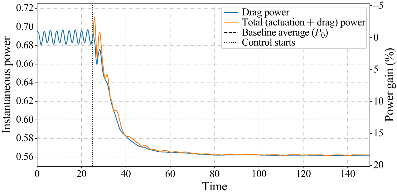Taking the time-averaged baseline flow drag power ($P_{0}=\tfrac {1}{2}\rho U_\infty ^3 D\langle C_{x,0}\rangle$) as reference, the actuation power $P_{act}$ peaks at $3.2\,\%$ of $P_0$ in the early stages of the first control phase, but only represents less than $0.1\,\%$ of $P_0$ on average in the second phase (see figure 10). Thus the total power expenditure – necessary both to counteract drag and to implement action – is temporarily higher than for the baseline flow. But it is quickly counterbalanced by the significant decrease of both drag and actuation powers during the second control phase. In the example shown in figure 10, the energy trade-off starts being beneficial $4.25$ time steps after the control starts, which is long before the flow stabilisation.

Figure 10.

Evolution of power expenditure throughout control. The drag power is the power necessary to withstand drag forces; the actuation power represents the power $P_{act}$ spent on action implementation. The power gain measures the instantaneous total power expenditure saved as a fraction of the averaged uncontrolled drag power.

The power-saving ratio ($PSR$) introduced by Protas & Wesfreid (Reference Protas and Wesfreid2002) is defined as the ratio of the gain in drag power to the time-averaged control power $\langle P_{act}\rangle$. In the quasi-steady controlled regime, $PSR\approx 143$ for $Re=120$, showing that the control obtained here is highly energy-efficient. For other Reynolds numbers, $PSR$ values are reported in table 1, and the values found are significantly higher than 1 even for the highest $Re$ considered. It is noteworthy that high $PSR$ values are very sensitive to $\langle P_{act}\rangle$ as it gets smaller. Thus, only the order of magnitude of the $PSR$ is meaningful in these cases.

It can be noticed that, for $Re=150$, Protas & Styczek (Reference Protas and Styczek2002) achieved extremely energy-efficient control, but with a lesser net drag reduction than the present study. On the other hand, the open-loop controls performed by Protas & Wesfreid (Reference Protas and Wesfreid2002), Bergmann et al. (Reference Bergmann, Cordier and Brancher2005) and Bergmann & Cordier (Reference Bergmann and Cordier2008) reach significant drag reduction but show low $PSR$ values. This highlights the difficulties of obtaining a control law that is efficient in terms of both net drag reduction and power consumption, which is achieved by the present DRL approach.

Note that quantitative comparisons of $PSR$ values from different studies is often not meaningful. For instance, in the case of cylinder rotation, the actuation power does not consider the inertia of the rotating cylinder (the mass of the cylinder is considered null). In the case of suction/blowing, the actuator efficiency is supposed to be perfect. This highlights that power-based comparisons between different actuation types may have a very limited relevance, and should only be considered quantitatively to distinguish highly efficient control ($PSR\gg 1$) from inefficient ($PSR=O(1)$) strategies.

It is interesting to note that, despite its high energy efficiency, the control policy is obtained without any explicit penalisation of the instantaneous control power. The actuation power expenditure is not directly included into the measured performance during learning. However, the reward $r_t$ is penalised by the time-averaged lift coefficient, which ensures parsimonious actions, since a strong action generates strong lift. Even though $C_l$ is averaged over one vortex shedding period, the periodicity of the flow varies (or even vanishes) during training, which makes a perfect compensation of the effects on $C_l$ of positive and negative actions very unlikely. As described early on, slightly non-zero average actions are systematically observed during the second control phase. Thus, a lack of convergence cannot account for this fact. Instead, an increase in the penalisation on lift through $\alpha$ causes a reduction of this constant component.

However, an increase in $\alpha$ has drawbacks. By trying several values within the range $[0;5]$, it has been observed that, for $Re=120$, the chosen value $\alpha =0.2$ is close to the optimal trade-off between pure performance and energy consumption. For both an increase or a decrease of $\alpha$, the $PSR$ decreases and the drag reduction shows a very slight decline. The slight negative effect on the $PSR$ when $\alpha$ decreases below $0.2$ can be explained by the reduction of the penalisation on large actions, thereby increasing the control power expenditure. On the other hand, an overly large value of $\alpha$ reduces the observed exploratory variance due to the strong disadvantage put on large-amplitude actions that are necessary in the early stages of the control to achieve a near-stabilisation of the flow. The search for the optimal $\alpha$ value has only been performed for $Re=120$, and the value of $0.2$ has been retained for other Reynolds-number values. Therefore, the $PSR$ values presented in table 1 may not be optimal and might be improved by a careful choice of $\alpha$. But from the results obtained for $Re=120$, it appears that $\alpha$ is not a sensitive parameter: it leads to negligible changes in drag reduction performance, and, for a wide range of $\alpha$ values, the $PSR$ value remains significantly higher than 1.

4.2. Analysis of the controlled flow

A common difficulty with deep learning approaches is the physical understanding of the results. Unfortunately, no simple action pattern has been noticed throughout the evaluations of the control strategy, whether it is for the first or second control phase. Unsuccessful attempts to reproduce this action behaviour with simpler linear controllers (simple gain and delayed response based on POD analyses) might indicate that complexity is required to reach the observed control efficiency. The projection of the controlled transient onto the three most energetic POD modes of the natural transient only captures at best $57\,\%$ of the energy of the flow (while they are enough to almost fully describe the natural transient). This shows that the controlled system is significantly more complex than the uncontrolled one, which may explain the encountered difficulties. While it is hard to explain precisely how the control policy acts on the flow to reduce drag, the present section nonetheless attempts to describe the control based on an a posteriori analysis of the flow.

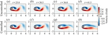
As studied by Nair et al. (Reference Nair, Taira, Brunton and Brunton2020), who used cylinder rotation or momentum injection parallel to the flow to impose an energy optimal phase-shift control, the drag reduction seen in the transient phase is caused by the delay in vortex shedding. This generates ‘elongated vortex structures’, which also stabilise the instantaneous recirculation bubble. Similar observations were made in our case. As shown by figure 11, the first phase of the control strategy is a fast transient from fully developed vortex shedding to a stabilised cylinder wake, where the actions trigger the shedding of vortices slightly earlier than the natural shedding. This results in longitudinally stretched and weaker vortical structures.

Figure 11.

Comparison of uncontrolled (a–d) and controlled (e–h) flows in the transient phase of the control strategy.

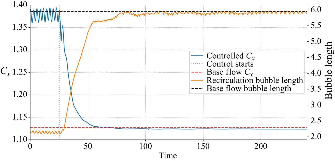
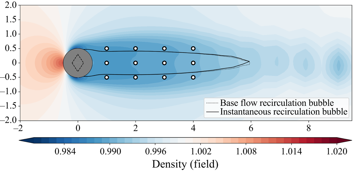
Once the flow has been stabilised and is nearly steady, its drag coefficient is very close to $C_{x,BF}$. Figure 12 compares the convergence of $C_x$ with the length of the instantaneous recirculation bubble. This length is multiplied by more than $2.5$ during the control phase and peaks at $99.5\,\%$ of the base-flow recirculation bubble length. The correlation of both the increase in the length of the recirculation bubble and the drag reduction is a well-known fact (Protas & Wesfreid Reference Protas and Wesfreid2002; Rabault et al. Reference Rabault, Kuchta, Jensen, Réglade and Cerardi2019). The recirculation bubble lengths found in this study are in good agreement with the reference literature (Zielinska et al. Reference Zielinska, Goujon-Durand, Dusek and Wesfreid1997; Protas & Wesfreid Reference Protas and Wesfreid2002). From time step 100 onwards, both base flow and controlled flow have a very similar recirculation bubble, as illustrated by figure 13. The ‘tail’ of the controlled bubble slowly flaps vertically with a very moderate displacement amplitude ($\Delta y <0.3$) at $St\approx 0.12$. This confirms that the control policy tends to lead the flow towards the base flow, the latter being an unstable optimum with respect to drag. The controlled flow reaches a small-amplitude cycle around this equilibrium point, driven by a slowly modulated, small-amplitude, quasi-periodic control action.

Figure 12.

Evolution of $C_x$ and of the length of the instantaneous recirculation bubble throughout time.

Figure 13.

Comparison of the base flow and the controlled flow recirculation bubbles once the flow is stabilised.

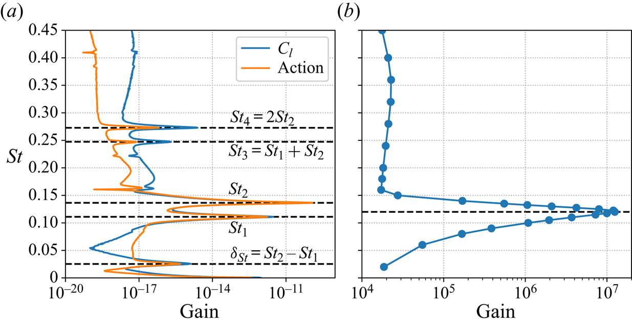
As shown in figure 14(a), the spectral analysis of the action during the second phase reveals two main oscillating components, $St_1\approx 0.11$ and $St_2\approx 0.14$, and three secondary peaks, at Strouhal numbers $\delta _{St}=St_2-St_1$, $St_3=St_1+St_2$ and $St_4=2St_2$, the latter having amplitudes at least two orders of magnitude lower than the main components. Since $\delta _{S_t}$ and $St_3$ are the marks of nonlinear coupling between the two main components, one can assume a nearly interaction-free superposition of the two main waves at $St_1$ and $St_2$. Their corresponding Fourier modes (not shown here) peak near the location of the ‘tail’ of the recirculation bubble.

Figure 14.

(a) Spectra of the lift coefficient $C_l$ and of the action during the second control phase. (b) Evolution of the optimal gain of the base-flow resolvent operator with the external forcing Strouhal number at $Re=120$.

Note that, in the stabilised phase, the state is close to the base flow and the actions are small, such that the flow evolves in a linear regime. The dominant Strouhal numbers of this phase are significantly lower than the natural vortex shedding frequency $St=0.18$. This may be easily understood by performing a resolvent analysis, which describes the frequency response of the flow in the vicinity of a steady state. If $\boldsymbol {q}$ denotes the flow state, $\boldsymbol {f}$ an external forcing and $\mathcal {N}$ the NS operator, then the NS equations may be written in compact form as

(4.1)

\begin{equation} \frac{\partial \boldsymbol{q}}{\partial t} = \mathcal{N}(\boldsymbol{q})+\boldsymbol{f}. \end{equation}

Decomposing the flow as the sum of the base flow $\boldsymbol {q}_{BF}$ and of a small perturbation $\boldsymbol {q}'$, and since the base flow is a steady solution ($\mathcal {N}(\boldsymbol {q}_{BF}) = 0$), the fluctuations $\boldsymbol {q}'$ are governed by the following first-order approximation:

(4.2)

\begin{equation} \frac{\partial \boldsymbol{q}'}{\partial t} -\boldsymbol{\mathsf{J}} \boldsymbol{q}' = \boldsymbol{f} \quad\text{with}\quad \boldsymbol{\mathsf{J}}=\frac{\partial \mathcal{N}}{\partial \boldsymbol{q}}( \boldsymbol{q}_{BF}). \end{equation}

The previous equation may then be Fourier-decomposed. Denoting the angular frequency by $\omega$, the identity matrix by $\boldsymbol {\mathcal {I}}$ and the Fourier-transformed variables by a hat notation, one has

(4.3)

\begin{equation} (\mathrm{i}\omega\boldsymbol{\mathcal{I}} - \boldsymbol{\mathsf{J}} )\hat{\boldsymbol{q}} ' = \hat{\boldsymbol{f}} \quad\Rightarrow\quad \hat{\boldsymbol{q}} ' = \underbrace{(\mathrm{i}\omega\boldsymbol{\mathcal{I}} - \boldsymbol{\mathsf{J}})^{{-}1}}_{\mathcal{R}} \, \hat{\boldsymbol{f}}, \end{equation}

with $\mathcal {R}$ being the resolvent operator. The highest singular value of $\mathcal {R}$, which is a function of $\omega$, gives the highest linear gain $\sigma$ that may be achieved through an external forcing (see e.g. Beneddine Reference Beneddine2017). Formally, it reads

(4.4)

\begin{equation} \sigma^2(\omega) = \max_{\hat{\boldsymbol{f}}} \frac{\|\hat{\boldsymbol{q}}'\|_{\boldsymbol{q}}}{\|\,\hat{\boldsymbol{f}}\|_{\boldsymbol{f}}}, \end{equation}

with $\|\cdot \|_{\boldsymbol {q}}$ and $\|\cdot \|_{\boldsymbol {f}}$ representing norms on the response and forcing spaces, respectively (classically associated with the kinetic energy for the response, and the $L_2$-norm for the forcing).

As illustrated by figure 14(b), the highest optimal gain is obtained for $St=0.12$ (consistently with Barkley (Reference Barkley2006) and Jin et al. (Reference Jin, Illingworth and Sandberg2019)) and the flow is responsive to only a narrow range of Strouhal numbers (below 0.15). It is therefore not surprising that the values associated with the control fall within this range. 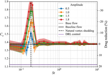But interestingly, the control avoids the highest gain frequency, and the particular selection of the two specific frequencies $St_1=0.11$ and $St_2=0.14$ remains an open question. To our knowledge, this is not reminiscent of any existing work related to the linear control of vortex shedding near the base flow. It is worth noting that both control time step and action interpolation have a negligible effect on the spectra since the control frequency is approximately $30$ times larger than $St_2$. Thus, there is no effect of aliasing and no significant distortion due to the interpolation method.

4.3. Robustness

4.3.1. Reynolds robustness

An assessment of the control policy robustness across a range of Reynolds numbers has been performed, using batches of 10 test cases having different random weight initialisation. This issue is tackled in the study of Atam et al. (Reference Atam, Mathelin and Cordier2016), where gain-scheduled controllers are evaluated on a cylinder flow with time-varying Reynolds number. Unlike Tang et al. (Reference Tang, Rabault, Kuhnle, Wang and Wang2020), who trained their policy on several Reynolds-number values ($100$, $200$, $300$ and $400$) and evaluated it on a mix of ‘seen’ and ‘unseen’ Reynolds numbers, our policy has been trained on a single Reynolds-number value $Re=120$, and evaluations have been performed on a range spanning from $Re=100$ to $216$ and compared with cases specifically trained on those Reynolds numbers. As illustrated by figure 3, this range of Reynolds numbers corresponds to a variation in vortex shedding Strouhal number of around $18\,\%$. Moreover, the non-dimensional amplitude of the pressure fluctuation displays a variation of a factor 2 between the two extreme $Re$ values considered. This shows that the dynamics of the flow, although not radically different, is still noticeably altered in this range of Reynolds number, such that the robustness is tested in actual off-design conditions.

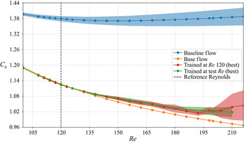
Figure 15 shows that the control is remarkably robust. Note that, as previously introduced, the flow state is made non-dimensional by the reference density $\rho _\infty$, upstream velocity $U_\infty$ and static temperature $T_\infty$. Reference velocities, pressures and case geometry (cylinder diameter and sensor location) being held constant is decisive for the robustness of the control policy. This ensures indeed a nearly constant convection time between sensors and comparable variation amplitudes both for sensors (on pressure) and for actuators (on mass flow) across the different Reynolds numbers considered. The only varying factor between different Reynolds-number flows is the change in vortex shape, their relative strength and organisation. The policy, acting only as a function of the current observation $s_t$, is insensitive to the variation in the von Kármán vortex street convection velocity. It is hence only affected by the change in instantaneous form of the flow structures, and the present results prove that the control law handles these changes very well.

Figure 15.

Robustness to a Reynolds-number variation. The best case (among 10 test cases) trained at $Re=120$ is tested at different Reynolds numbers (red curve). Its performance is compared to the best control policy (among 10 test cases) specifically trained at the test Reynolds number (green curve). Shaded areas represent the standard deviation of the controlled drag coefficient $C_x$.

Non-dimensionalisation also circumvents the issue of neural network input normalisation. Once neural networks’ weights and biases are tuned to adapt to the range of input values, they remain appropriately tuned, as this range does not overly change across Reynolds numbers. Tang et al. (Reference Tang, Rabault, Kuhnle, Wang and Wang2020) used the same non-dimensionalisation scheme. Thus, even though their deep learning algorithm is different, the robustness they observed may be explained by the fact that the policy is robust over a wide range of Reynolds numbers even with a single Reynolds-number training. Adding several other Reynolds numbers in the training marginally improves an already strong robustness.

This robustness is very promising for future experimental exploitation of deep learning for flow control, since flow conditions are subject to uncertainties in experiments. Should one attempt to use a computational fluid dynamics (CFD) trained policy to control an actual experimental case, it may be interesting to consider transfer learning, which consists in retraining only specific layers of the network rather than the whole model to quickly adapt it to a slightly different configuration, without restarting from scratch. Several studies have been done in the image processing community on the topic (Huh, Agrawal & Efros Reference Huh, Agrawal and Efros2016) and should be considered for future work.

Figure 15 also shows better robustness for lower Reynolds numbers than for higher ones (compared to the $Re$ of training). One of the reasons may be that the chosen sensor layout, fixed across all cases, covers more of the base-flow recirculation bubble for lower Reynolds numbers. It has been shown indeed that its length increases with the Reynolds number. The $12$-sensor layout spans over $75\,\%$ of the recirculation region at $Re =100$, but only $55\,\%$ at $Re=216$.

4.3.2. Observation noise robustness

Assessing the tolerance of the control strategy to measurement errors is a key point in the transposition of that method to real-world experiments, where measurement noise is unavoidable. Noise robustness is therefore important in the perspective of transfer learning from a numerically trained case (without noise) to an experimental set-up. To this end, the robustness of a zero-training-noise policy has been assessed and compared with policies trained on noisy data using batches of 20 randomly initialised test cases as previously done for the assessment of the Reynolds-number robustness. Added noise is parametrised using a relative amplitude $\sigma$. Noisy observations $\tilde {s}_t$ are computed as

(4.5)

\begin{equation} \tilde{s}_t = s_t + \bar{s}_t\sigma\mathcal{N}(\,\cdot{\mid} 0,1), \end{equation}

where $\bar {s}_t$ is the average pressure over all sensors at time $t$, which is found to be relatively steady, and $\mathcal {N}(\,\cdot{\mid}0,1)$ is a standard random normal probability distribution.

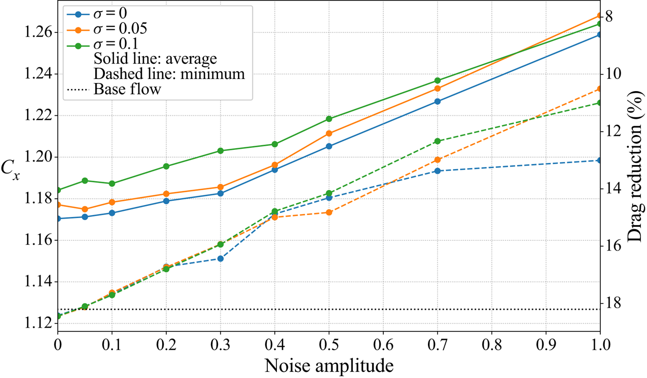
Figure 16 compares the performances of policies trained at different noise levels $\sigma$ and evaluated on a range of noise levels from $0$ to $1$. One can notice that the level of training noise does not seem to impact performances in a significant manner up to $\sigma =0.5$, which corresponds to very noisy measurements that certainly exceed the actual noise one may expect in most experiments (see figure 17). Unexpectedly, figure 16 tends to show that a zero-training-noise policy seems overall slightly more robust to noise than others at different training noise levels. Therefore, in the present case, it is unnecessary to account for measurement noise during the training, which is once again promising for the possible transfer of CFD-trained models to experiments.

Figure 16.

Robustness to Gaussian noise on observations. Each curve represents the mean (solid line) or the best (dashed line) performance in drag coefficient of a 20 test-case batch trained with noise levels from $\sigma =0$ to $\sigma =0.1$ and evaluated on noise levels ranging from $\sigma =0$ to $\sigma =1$.

Figure 17.

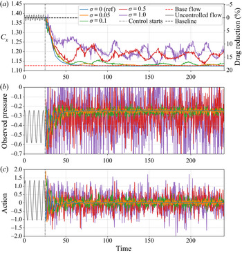
Robustness to Gaussian noise on observations for a policy trained without noise ($\sigma =0$). (a) Evolution of $C_x$ throughout time, for different noise levels. (b) Noisy pressure signal $s_0$ located in $(1,0.5)$. (c) Corresponding action taken by the actor.

Figure 17 illustrates this robustness throughout time for a policy trained with $\sigma =0$. Despite large noise disturbances, the control policy achieves good performances. Even with extreme noise levels such as $\sigma =1$, the drag reduction reaches approximately $12\,\%$ on average. This may be explained by the feedback characteristic of the problem that enables efficient error correction from one control step to the next.Both observation and action signal-to-noise ratios ($SNR$) are assessed on the second control phase (having steady statistics) as

(4.6)

\begin{equation} SNR=\frac{\text{noise-free variation amplitude}}{\text{noise standard deviation}}. \end{equation}

Action noise is defined as the difference between the action computed using noisy observations and the action based on noise-free measurements.

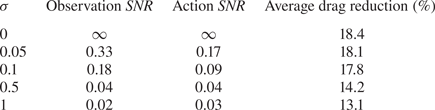
Results are reported in table 2. Note that the apparent discrepancies between $SNR$ and $\sigma$ values are due to the definition of each quantity: $SNR$ values are computed considering the amplitude of variation of the signal, thus excluding the signal's time-averaged value, while the noise level driven by $\sigma$ is measured as a fraction of the signal value, including its constant component. It can be seen that the action $SNR$ has the same order of magnitude as the observation $SNR$, with their ratio ranging between $0.7$ and $2$. In particular, the $SNR$ of observations and actions become closer as the level of noise increases. This highlights the robustness of the policy, which does not diverge from optimal actions due to spurious fluctuations within the observations. The errors do not accumulate over time and the closed-loop system seems able to rectify the previous erroneous action to contain the deviation from the optimal controlled flow state. The policy is therefore sufficiently insensitive to input errors in that range of noise levels to ensure a strong robustness. In addition, it is possible that the decorrelation of these errors between each measurement helps to mitigate the effects of the noise.

Table 2.

Noise robustness comparison.

4.4. Impact of the sensor number and location on the control performance

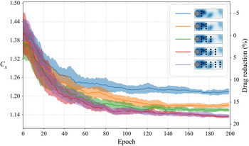
As introduced previously, the optimisation of both the number and location of sensors is a widely explored domain. In this section, a systematic study on sensor configurations within a $3 \times 5$ grid-like layout ($(x,y)\in \{1,2,3,4,5\}\times \{-0.5,0,0.5\}$) is performed. Figure 18 illustrates the learning curves of 10-case batches having from three to $15$ sensors. The addition of the second and third columns of sensors (located at $x=2$ and $x=3$) yields a significant gain in performance, and one can notice that $12$- and $15$-sensor layouts have a very similar average performance. Thus it is possible to conclude that the three additional sensors (located at $x=5$) are not useful to the control strategy.

Figure 18.

Ten-case batch-averaged learning curves for five different sensor layouts (as shown in the key at top right). Shaded areas represent the standard deviation of the corresponding plotted quantities. Each $C_x$ value is averaged over the whole epoch, including the transient from developed vortex shedding to controlled flow. This explains the discrepancy with pure performance values on $C_x$ introduced earlier.

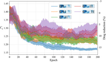
Figure 19 shows the effect of the location of pressure observations, for an array of six sensors that are displaced in the streamwise direction. This time, the importance of the first sensor column (located at $x=1$) is demonstrated by the noticeable gain in drag reduction between the first two layouts (blue and yellow curves). The importance of the third sensor column ($x=3$) is once again stressed by the decrease in performance between the green and red curves. Within this predefined combinatorial set, this partial study highlights the relevance of sensors closest to the cylinder. These first preliminary tendencies are confronted in the next section with the results from the newly proposed S-PPO-CMA algorithm that is designed to provide an optimised sensor location for the control.

Figure 19.

Ten-case batch-averaged learning curves for a further five different sensor layouts (as shown in the key at top right). Shaded areas represent the standard deviation of the corresponding plotted quantities. Each $C_x$ value is averaged over the whole epoch, including the transient from developed vortex shedding to controlled flow. This explains the discrepancy with pure performance values on $C_x$ introduced earlier.

4.5. Optimised choice of sensors: results from the S-PPO-CMA algorithm

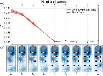
The S-PPO-CMA algorithm, described in § 3, is used here to derive optimised sensor placement for any allocated number of sensors ranging from one to nine, within the imposed $15$-sensor grid-like pattern. The number of sensors at convergence is indirectly controlled through the value of the $L_0$ regularisation constant $\lambda$, which balances the gradients of both $\mathcal {L}_{\pi _s}$ (performance loss) and $\mathcal {L}_c$ (complexity loss). Figure 20 shows the achievable drag reduction with respect to the number of sensors $i$ and the corresponding sensor layout $l_i$. Note that, due to the symmetry of the configuration, there always exist pairs of symmetric layouts that achieve identical performances. The S-PPO-CMA algorithm randomly outputs one of the two optimised layouts for each value of $\lambda$, but only one layout is displayed in the figures for simplicity.

Figure 20.

Evolution of both drag reduction and optimised sensor layout with the number of sensors. Layout thumbnails $l_1$ to $l_9$ are rotated $90^\circ$ clockwise.

With a single sensor, the drag reduction is around $11\,\%$ and it peaks at approximately $18\,\%$ for five sensors or more. The sensor pattern's tendency to fill without relocating existing sensors, meaning that $l_i\subset l_{j>i}$, is a sign of convexity of this problem in the sense that any combination of the optimised layout set is also part of this set. It is interesting to notice that, starting from the five-sensor optimised layout, the addition of more sensors does not improve drag reduction, which makes this five-sensor layout the optimised trade-off between performance and sensor set-up complexity. To our knowledge, this layout is not reminiscent of anything used in the large number of existing studies on the control of 2-D cylinder wakes. Thus, this highlights the usefulness of the S-PPO-CMA algorithm, since optimised sensor placement is, even in such a simple case, not particularly intuitive.

The centreline locations ($y=0$) do not appear relevant for the control, since the corresponding sensors are never selected by the algorithm. A possible explanation may be that these sensors cannot provide information relative of the instantaneous asymmetry of flow, and are thus unfit to choose the action's sign. The first two layouts $l_1$ and $l_2$ validate the importance of the first sensor column, and the selection of sensors shows a weaker importance of locations beyond $x=4$. This is in line with the conclusions of § 4.4.

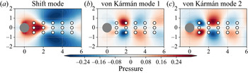
As discussed in the introduction, many studies optimise sensor placement based on the linear framework of POD, with the underlying idea that, the better the estimation of mode coefficients, the better the reconstruction and control performance. They naturally often choose locations where the POD modes are strong. Figure 21 illustrates the superimposition of the sensor locations, with the first three POD modes derived from the natural transient from base flow to fully developed vortex shedding. These three modes account for more than $95\,\%$ of the transient's energy. Despite the fact that these modes are only valid for control trajectories that stay close to this natural transient, the choice of $l_2$ seems reasonable, as it allows estimations of both shift mode and second vortex shedding mode simultaneously, since sensors are close to the extrema of these modes (refer to figure 21a,c). The second column of sensors appears less able to provide relevant information on the shift mode. Figure 21 also confirms that the centreline sensors are not suitable to estimate von Kármán modes, which account for the instantaneous asymmetry of the vortex shedding.

Figure 21.

Comparison of the sensor locations with the first three POD modes of a natural transient from base flow to fully developed vortex shedding.

Comparing the second and third layouts $l_2$ and $l_3$, it appears that, given the first two probe locations, an additional sensor is preferred in the third column rather than in the second. This might be because this layout provides a better ‘coverage’ of the instantaneous recirculation bubble. Additionally, despite the lack of mean flow symmetry during the transient phase of control, sensors tend to concentrate on a single streamwise row. From a POD-based control viewpoint, this may not be optimal for reconstruction of modes. This shows the strength of the present approach: an estimation of the full flow field (or the dominant POD modes) is likely not to be needed for control. Therefore, searching for points that allow such a full reconstruction may be suboptimal. In that context, favouring a precise vortex tracking whose centre travels in the vicinity of the external sensor rows over a more complete estimation of the wake may lead to better performance.

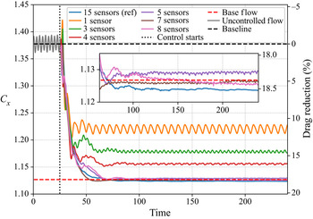
Figure 22 compares the performances of some of the previously found sensor layouts throughout time. It confirms that, as from five sensors, optimal performance (${\sim }18\,\%$) is reached. All configurations show a comparable transient phase that stops earlier in both time and drag reduction for the sparsest sensor configurations. Despite an already significant drag reduction, layout $l_1$ seems unable to notably stabilise the vortex shedding instability. A much better steadiness is achieved with three, four and more sensors.

Figure 22.

Performance comparison for different optimised sensor layouts.

5. Conclusion

In this study, PPO-CMA, implemented on a laminar 2-D cylinder case study, discovered efficient nonlinear control strategies with only 12 pressure sensors in the cylinder's wake. A drag reduction of $18.4\,\%$ is reached for $Re =120$. Comparable performances are achieved for other values of $Re$, which match state-of-the-art control performances. The control strategy has been analysed a posteriori and split into two distinct phases. After a rapid transient phase where large-amplitude actions bring the mean flow close to the base flow, the policy simply keeps the controlled flow on a small-amplitude limit cycle. The policy uses weaker actions, whose temporal spectrum is dominated by two distinct frequencies, both close to the base flow's resonance frequency. This translates to a temporary disadvantageous energy expenditure, which quickly becomes beneficial with a $PSR$ of the order of ${O}(100)$ for the whole range of $Re$ considered.

The robustness with respect to a variation in Reynolds number and measurement noise has also been quantified. It has been demonstrated that a policy trained at $Re=120$ exhibits near-optimal performances that match the drag reductions achieved by specifically trained policies on Reynolds numbers in the range $[100;216]$. Such robustness is in part explained by the chosen non-dimensionalisation scheme in the case study. The impact of measurement noise has been assessed by both training policies with different noise levels and by evaluation of these policies on different levels of noisy observations. It has been concluded that, overall, the control is very robust, yet noise-free trained policies seem slightly more robust than those trained on noisy data. The actor takes advantage of both the decorrelation of noise between observations and the closed-loop nature of the problem to demonstrate efficient control of a noisy environment. Those two aspects show interesting possibilities for direct application of reinforcement-based feedback control to real-world cases. As long as forward passes in the actor neural structure comply with real-time constraints, such control policies are deemed relevant for experiments. In that case, transfer learning could be used to benefit from a synergistic coupling between numerical simulation and experiments. The demonstrated robustness of the derived policies suggests an interesting potential for DRL-based control methods in complex flows that yet needs to be completely assessed in future studies and applications.

An optimisation of the number of sensors has also been performed while preserving performances. After a first coarse systematic study showing the importance of having sensors close to the cylinder, S-PPO-CMA has been introduced and implemented on the test case. This new algorithm, discovering optimised sensor layouts for reinforcement-based control, selects the most relevant sensors and discards redundant and irrelevant ones. Thus, the number of sensors has been reduced to only five while keeping state-of-the-art performance. The obtained sensor layout has been compared with both the outcomes of our systematic study and the conclusions of other linear (mostly POD-based) studies. Several explanations have been proposed to back the observed consistency of these results. This optimisation is based on a coarse grid of sensors. A denser layout, covering a larger portion of the flow, has been studied (not shown) and gives similar results. So far, the only limitation identified to the extension of this method to three dimensions and/or more complex flows is the computational cost required to generate enough training data. However, the present study highlighted an important drawback of this approach. As discussed earlier, the interpretation of control policies even on a simple case is non-trivial. With a growing interest in real-world applications, the explainability and interpretability of neural networks need to be improved, especially for multi-input–multi-output systems. As such, these topics are gaining increasing attention. Future analysis methods may improve our understanding of these control laws and their interactions with the flow.

A way to further improve the performances of the present approach may be by including time-recurrent neural structures, considering multiple successive measurement snapshots at once, such as long short-term memory. Despite being harder to train, these networks could enable efficient control with even fewer sensors and an increased robustness to noise. Another interesting direction to explore may be the use of surface-mounted sensors only, similarly to what Atam et al. (Reference Atam, Mathelin and Cordier2016) did and which is a more realistic set-up. It is likely that restricting the sensor location limits the performance of the control. It may be interesting to attempt to overcome this issue by the use of more advanced strategies. As shown by He et al. (Reference He, Glowinski, Metcalfe, Nordlander and Periaux2000), this could mean seeking other mean flow configurations with, for instance, induction of a reverse von Kármán street (Bergmann, Cordier & Brancher Reference Bergmann, Cordier and Brancher2006). However, this may require an actuation system similar to what Tang et al. (Reference Tang, Rabault, Kuhnle, Wang and Wang2020) did and a reduced energy efficiency.

Acknowledgements

The authors would like to thank J. Rabault for valuable discussions and advice.

Funding

This work is funded by the French Agency for Innovation and Defence (AID) via a PhD scholarship. Their support is gratefully acknowledged.

Declaration of interests

The authors report no conflict of interest.

Appendix A. Open-source code

The source code proposing an implementation of the S-PPO-CMA algorithm is available at the following URL: https://bitbucket.org/Romain_Paris/drl_cylinder.

Appendix B. Open-loop control of the test case

A sinusoidal open-loop control strategy has been tested on the test case of the study. The action is computed as: $a_t =\alpha \sin (\varOmega t)$, $\alpha \in [-2;2]$ being the amplitude of the forcing and $\varOmega \in [0.002;10]$ the Strouhal number of the forcing. As shown by figure 23, open-loop periodic control exhibits poor results compared to the DRL-learned control policy (purple line).

Figure 23.

Evolution of the drag coefficient for periodic (sinusoidal) action with various amplitudes and Strouhal numbers. Shaded areas represent the standard deviation of the drag coefficient. These values are averaged over 10 randomly initialised test cases.

Appendix C. PPO, PPO-CMA and S-PPO-CMA learning algorithms

Given a partial state $s_t$ and under a policy $\pi$, the advantage value $A^\pi (a_t,s_t)$ compares the value ($R_t$) of a specific action $a_t$ with the expected value of a randomly selected action according to $\pi (\cdot ,s_t)$. The latter is simply $V^\pi (s_t)$, the state value computed by the critic neural network $V$, and is an estimator of the expected return $\mathbb {E}_{\pi }[\sum _\tau \gamma ^\tau r_\tau ]$ following policy $\pi$. The advantage estimates ‘how much better’ $a_t$ is compared to the ‘average’ action sampled following $\pi$: $A^\pi (a_t,s_t)= R_t-V^\pi (s_t)$. A more stable method of estimating advantage, generalised advantage estimation (GAE; Schulman et al. Reference Schulman, Moritz, Levine, Jordan and Abbeel2015b), depending on an extra parameter $\lambda _{GAE}$, is used here. PPO and its variants rely on the estimation of the advantage function and use advantage values as weights for the computation of gradients. Concerning PPO, the policy $\pi _\theta (\cdot ,s_t)$ follows a random normal distribution whose mean $\mu _\theta (s_t)$ is the output of a neural network $\pi$ ($\theta$ being its weights/biases) and standard deviation $\sigma$ is a predefined hyper-parameter. The surrogate loss computed during policy update is

(C 1)

\begin{equation} \mathcal{L}_{PPO}(t) = \min (r_\theta,\text{clip}(r_\theta,1-\varepsilon,1+\varepsilon) )A^\pi(a_t,s_t), \end{equation}

where

(C2a,b)

\begin{equation} r_\theta(t) = \frac{\pi_\theta(a_t,s_t)}{\pi_{\theta_{old}}(a_t,s_t)} \quad\text{and}\quad \text{clip} (a,b,c) = \min (\max(a,b ),c), \end{equation}

with $\theta _{old}$ being the weights of $\pi$ before update and $\varepsilon$ a clipping hyper-parameter. Algorithm describes the steps of PPO, with $\phi$ being the weights and biases of $V$.

Algorithm 1

PPO algorithm.

PPO-CMA (Hämäläinen et al. Reference Hämäläinen, Babadi, Ma and Lehtinen2020) relies on a similar loss estimation technique, but uses two unclipped surrogate objectives. The standard deviation of the policy $\pi _\theta$ is, this time, also an output of the actor $\pi$. The latter is then trained twice per update phase using two different losses $\mathcal {L}_{PPOCMA}^\sigma$ and $\mathcal {L}_{PPOCMA}^\mu$. With PPO being known for its instability in policy updates due to negative advantages, PPO-CMA uses a mirroring technique to consider the information brought by negative advantage samples:

(C 3)

\begin{gather} \mathcal{L}_{PPOCMA}^\sigma(t) = \delta_{A^\pi>0}A^\pi(a_t,s_t) \pi_\theta(a_t,s_t), \end{gather}

(C 4)

\begin{gather} \mathcal{L}_{PPOCMA}^\mu(t) = \delta_{A^\pi>0}A^\pi(a_t,s_t) \pi_\theta(a_t,s_t) - \delta_{A^\pi<0}A^\pi(a_t,s_t) \pi_\theta(\mu_t-2a_t,s_t)Z(a_t-\mu_t), \end{gather}

with

(C 5)

\begin{equation} \delta_{f(x)}= \left\{\begin{matrix}1, & \text{if } f(x)\text{ is true},\\ 0, & \text{ otherwise},\end{matrix}\right. \end{equation}

where $Z$ is a Gaussian kernel damping function, which vanishes when $\|a_t-\mu _t\|\rightarrow \infty$. To ensure a more stable convergence of $\sigma$, $\mathcal {L}_{PPOCMA}^\sigma$ is estimated on a randomly sampled history buffer $\mathcal {B}$ that contains all the information of the past $H$ epochs of training. Algorithm describes the steps of PPO-CMA.

Algorithm 2

PPO-CMA algorithm.

The training of S-PPO-CMA (described in § 3) is similar to that of the standard PPO-CMA. An additional loss $\mathcal {L}_{{sparse}}$ is defined to train $\boldsymbol {\alpha }$ values. This contains a Tikhonov matrix $\boldsymbol {\varGamma }$, which penalises correlations between observations. This matrix $\boldsymbol {\varGamma }$ is diagonal and for a predefined correlation threshold $\delta _{corr}$:

(C 6)

\begin{gather} C_i \equiv \{\,j\neq i \mid \text{corr}(s_i,s_j)>\delta_{corr} \}, \end{gather}

(C 7)

\begin{gather} \varGamma_{ii} = \left\{\begin{matrix} 1, & \text{if } C_i \neq \emptyset\text{ and }\exists\ j\in C_i\ {\rm s.t.}\ \alpha_j > \alpha_i, \\ 0, & \text{otherwise},\end{matrix}\right. \end{gather}

where $\text {corr}(s_i,s_j)$ is the correlation of $s_i$ and $s_j$ over the current epoch.

The substitute vector $\bar {\boldsymbol {s}}$ can be seen as a baseline. There is an advantage in gradient accuracy to choose a slowly updated average of the observation vector as baseline. Let us consider:

(C 8)

\begin{gather} \boldsymbol{\nabla}_{\alpha}\mathcal{L}_{ \pi_s}(\theta_s,\boldsymbol{\alpha}) = \underbrace{\text{sign}[\mu_s(\boldsymbol{s},\theta_s,\boldsymbol{\alpha}) - \mu^*(\boldsymbol{s})]}_{\delta}\boldsymbol{\nabla}_\alpha\mu_s (\boldsymbol{s},\theta_s,\boldsymbol{\alpha} ), \end{gather}

(C 9)

\begin{gather} \boldsymbol{\nabla}_{\alpha}\mathcal{L}_{ \pi_s}(\theta_s,\boldsymbol{\alpha}) = \delta \boldsymbol{\nabla}_{\tilde{\boldsymbol{s}}} \pi_{s,\sigma}(\theta_s,\tilde{\boldsymbol{s}} )\odot\boldsymbol{\nabla}_\alpha \tilde{\boldsymbol{s}} \quad\text{with}\quad \tilde{\boldsymbol{s}} = (\boldsymbol{s}-\bar{\boldsymbol{s}})\odot f(\boldsymbol{u},\boldsymbol{\alpha})+\bar{\boldsymbol{s}}, \end{gather}

(C 10)

\begin{gather} \boldsymbol{\nabla}_\alpha \tilde{\boldsymbol{s}} = (\boldsymbol{s}-\bar{\boldsymbol{s}})\odot\boldsymbol{\nabla}_\alpha f(\boldsymbol{u},\boldsymbol{\alpha}). \end{gather}

Thus one obtains

(C 11)

\begin{equation} \boldsymbol{\nabla}_{\alpha}\mathcal{L}_{ \pi_s}(\theta_s,\boldsymbol{\alpha}) = \delta \boldsymbol{\nabla}_{\tilde{\boldsymbol{s}}} \pi_{s,\sigma}(\theta_s,\tilde{\boldsymbol{s}} )\odot\boldsymbol{\nabla}_\alpha f(\boldsymbol{u},\boldsymbol{\alpha})\odot (\boldsymbol{s}-\bar{\boldsymbol{s}}). \end{equation}

If $\bar {\boldsymbol {s}} = 0$, for the values of $\boldsymbol {u}$ where $\boldsymbol {\nabla }_\alpha \, f(\boldsymbol {u},\boldsymbol {\alpha })\neq 0$, the amplitude of the gradient is proportional to the average value of $\boldsymbol {s}$. If there is an important disparity in observation averages (i.e. $\textrm {avg}(s_i)\gg \textrm {avg}(s_j)$), $\alpha _i$ will be updated much faster than $\alpha _j$, which is not desired. Furthermore, for ‘small’ batches, any correction based on the batch average (using $\textrm {avg}(\boldsymbol {s})$ instead of $\bar {\boldsymbol {s}}$) introduces a bias due to the lack of convergence of the epoch-averaged estimator avg. A slowly updated baseline for $\bar {\boldsymbol {s}}$ is thus necessary.

Appendix D. Numerical hyper-parameters

Table 3 presents the main numerical parameters of both the simulated case and the learning algorithm, with the notation used in the article (if introduced).

Table 3.

Additional numerical parameters.

References

REFERENCES

Abadi, M., Barham, P., Chen, J., Chen, Z., Davis, A., Dean, J., Devin, M., Ghemawat, S., Irving, G. & Isard, M. 2016 Tensorflow: a system for large-scale machine learning. In 12th USENIX Symposium on Operating Systems Design and Implementation (OSDI 16), pp. 265–283.Google Scholar

Arakeri, J.H. & Shukla, R.K. 2013 A unified view of energetic efficiency in active drag reduction, thrust generation and self-propulsion through a loss coefficient with some applications. J. Fluids Struct. 41, 22–32.CrossRef Google Scholar

Atam, E., Mathelin, L. & Cordier, L. 2016 Identification-based closed-loop control strategies for a cylinder wake flow. IEEE Trans. Control Syst. Technol. 25 (4), 1488–1495.CrossRef Google Scholar

Baker, B., Kanitscheider, I., Markov, T., Wu, Y., Powell, G., McGrew, B. & Mordatch, I. 2019 Emergent tool use from multi-agent autocurricula. arXiv:1909.07528.Google Scholar

Barkley, D. 2006 Linear analysis of the cylinder wake mean flow. Europhys. Lett. 75 (5), 750.CrossRef Google Scholar

Beintema, G., Corbetta, A., Biferale, L. & Toschi, F. 2020 Controlling Rayleigh–Bénard convection via reinforcement learning. J. Turbul. 21 (9–10), 585–605.Google Scholar

Belus, V., Rabault, J., Viquerat, J., Che, Z., Hachem, E. & Reglade, U. 2019 Exploiting locality and translational invariance to design effective deep reinforcement learning control of the 1-dimensional unstable falling liquid film. AIP Adv. 9 (12), 125014.CrossRef Google Scholar

Beneddine, S. 2017 Characterization of unsteady flow behavior by linear stability analysis. PhD thesis, Université Paris-Saclay.Google Scholar

Benoit, C., Péron, S. & Landier, S. 2015 Cassiopee: a CFD pre-and post-processing tool. Aerosp. Sci. Technol. 45, 272–283.CrossRef Google Scholar

Bergmann, M. & Cordier, L. 2008 Optimal control of the cylinder wake in the laminar regime by trust-region methods and POD reduced-order models. J. Comput. Phys. 227 (16), 7813–7840.CrossRef Google Scholar

Bergmann, M., Cordier, L. & Brancher, J.-P. 2005 Control of the cylinder wake in the laminar regime by trust-region methods and POD reduced order models. In Proceedings of the 44th IEEE Conference on Decision and Control, pp. 524–529.Google Scholar

Bergmann, M., Cordier, L. & Brancher, J.-P. 2006 On the generation of a reverse Von Kármán street for the controlled cylinder wake in the laminar regime. Phys. Fluids 18 (2), 028101.CrossRef Google Scholar

Braza, M., Chassaing, P.H.H.M. & Minh, H.H. 1986 Numerical study and physical analysis of the pressure and velocity fields in the near wake of a circular cylinder. J. Fluid Mech. 165, 79–130.CrossRef Google Scholar

Bright, I., Lin, G. & Kutz, J.N. 2013 Compressive sensing based machine learning strategy for characterizing the flow around a cylinder with limited pressure measurements. Phys. Fluids 25 (12), 127102.CrossRef Google Scholar

Brockman, G., Cheung, V., Pettersson, L., Schneider, J., Schulman, J., Tang, J. & Zaremba, W. 2016 OpenAI gym. arXiv:1606.01540.Google Scholar

Brunton, S.L. & Noack, B.R. 2015 Closed-loop turbulence control: progress and challenges. Appl. Mech. Rev. 67 (5), 050801.CrossRef Google Scholar

Brunton, S.L., Noack, B.R. & Koumoutsakos, P. 2020 Machine learning for fluid mechanics. Annu. Rev. Fluid Mech. 52, 477–508.CrossRef Google Scholar

Bucci, M.A., Semeraro, O., Allauzen, A., Wisniewski, G., Cordier, L. & Mathelin, L. 2019 Control of chaotic systems by deep reinforcement learning. Proc. R. Soc. A 475, 20190351.Google Scholar

Chen, Z. & Aubry, N. 2005 Active control of cylinder wake. Commun. Nonlinear Sci. Numer. Simul. 10 (2), 205–216.CrossRef Google Scholar

Cho, K., Van Merriënboer, B., Gulcehre, C., Bahdanau, D., Bougares, F., Schwenk, H. & Bengio, Y. 2014 Learning phrase representations using RNN encoder-decoder for statistical machine translation. arXiv:1406.1078.CrossRef Google Scholar

Cohen, K., Siegel, S. & McLaughlin, T. 2006 A heuristic approach to effective sensor placement for modeling of a cylinder wake. Comput. Fluids 35 (1), 103–120.CrossRef Google Scholar

Cohen, K., Siegel, S., Seidel, J., Aradag, S. & McLaughlin, T. 2012 Nonlinear estimation of transient flow field low dimensional states using artificial neural nets. Expert Syst. Appl. 39 (1), 1264–1272.CrossRef Google Scholar

Colabrese, S., Gustavsson, K., Celani, A. & Biferale, L. 2017 Flow navigation by smart microswimmers via reinforcement learning. Phys. Rev. Lett. 118 (15), 158004.CrossRef Google Scholar PubMed

Curtiss, C.F. & Hirschfelder, J.O. 1952 Integration of stiff equations. Proc. Natl Acad. Sci. USA 38 (3), 235.CrossRef Google Scholar PubMed

Dandois, J., Garnier, E. & Pamart, P.-Y. 2013 NARX modelling of unsteady separation control. Exp. Fluids 54 (2), 1445.CrossRef Google Scholar

Dandois, J., Mary, I. & Brion, V. 2018 Large-eddy simulation of laminar transonic buffet. J. Fluid Mech. 850, 156–178.CrossRef Google Scholar

DeVries, L. & Paley, D.A. 2013 Observability-based optimization for flow sensing and control of an underwater vehicle in a uniform flowfield. In 2013 American Control Conference, pp. 1386–1391.Google Scholar

Edwards, J.R. & Liou, M.-S. 1998 Low-diffusion flux-splitting methods for flows at all speeds. AIAA J. 36 (9), 1610–1617.CrossRef Google Scholar

Foures, D.P.G., Dovetta, N., Sipp, D. & Schmid, P.J. 2014 A data-assimilation method for Reynolds-averaged Navier–Stokes-driven mean flow reconstruction. J. Fluid Mech. 759, 404–431.CrossRef Google Scholar

Fujisawa, N., Kawaji, Y. & Ikemoto, K. 2001 Feedback control of vortex shedding from a circular cylinder by rotational oscillations. J. Fluids Struct. 15 (1), 23–37.CrossRef Google Scholar

Gerhard, J., Pastoor, M., King, R., Noack, B., Dillmann, A., Morzynski, M. & Tadmor, G. 2003 Model-based control of vortex shedding using low-dimensional Galerkin models. In 33rd AIAA Fluid Dynamics Conference and Exhibit, p. 4262.Google Scholar

Gutmark, E.J. & Grinstein, F.F. 1999 Flow control with noncircular jets. Annu. Rev. Fluid Mech. 31 (1), 239–272.CrossRef Google Scholar

Hämäläinen, P., Babadi, A., Ma, X. & Lehtinen, J. 2020 PPO-CMA: proximal policy optimization with covariance matrix adaptation. In 2020 IEEE 30th International Workshop on Machine Learning for Signal Processing (MLSP), pp. 1–6. IEEE.CrossRef Google Scholar

Hansen, N. 2016 The CMA evolution strategy: a tutorial. arXiv:1604.00772.Google Scholar

Hansen, N., Müller, S.D. & Koumoutsakos, P. 2003 Reducing the time complexity of the derandomized evolution strategy with covariance matrix adaptation (CMA-ES). Evol. Comput. 11 (1), 1–18.CrossRef Google Scholar

He, J.-W., Glowinski, R., Metcalfe, R., Nordlander, A. & Periaux, J. 2000 Active control and drag optimization for flow past a circular cylinder: I. Oscillatory cylinder rotation. J. Comput. Phys. 163 (1), 83–117.CrossRef Google Scholar

He, K., Zhang, X., Ren, S. & Sun, J. 2016 Deep residual learning for image recognition. In Proceedings of the IEEE Conference on Computer Vision and Pattern Recognition, pp. 770–778.Google Scholar

Henderson, R.D. 1997 Nonlinear dynamics and pattern formation in turbulent wake transition. J. Fluid Mech. 352, 65–112.CrossRef Google Scholar

Huh, M., Agrawal, P. & Efros, A.A. 2016 What makes imagenet good for transfer learning? arXiv:1608.08614.Google Scholar

Jin, B., Illingworth, S.J. & Sandberg, R.D. 2019 Feedback control of vortex shedding using a resolvent-based modelling approach. arXiv:1909.04865.CrossRef Google Scholar

Kaiser, L., Babaeizadeh, M., Milos, P., Osinski, B., Campbell, R.H., Czechowski, K., Erhan, D., Finn, C., Kozakowski, P. & Levine, S. 2019 Model-based reinforcement learning for Atari. arXiv:1903.00374.Google Scholar

Kim, K., Kerr, M., Beskok, A. & Jayasuriya, S. 2006 Frequency-domain based feedback control of flow separation using synthetic jets. In 2006 American Control Conference, p. 6. IEEE.Google Scholar

Kingma, D.P. & Ba, J. 2014 Adam: a method for stochastic optimization. arXiv:1412.6980.Google Scholar

Leclerc, E., Sagaut, P. & Mohammadi, B. 2006 On the use of incomplete sensitivities for feedback control of laminar vortex shedding. Comput. Fluids 35 (10), 1432–1443.CrossRef Google Scholar

Leclercq, C., Demourant, F., Poussot-Vassal, C. & Sipp, D. 2019 Linear iterative method for closed-loop control of quasiperiodic flows. J. Fluid Mech. 868, 26–65.CrossRef Google Scholar

Louizos, C., Welling, M. & Kingma, D.P. 2017 Learning sparse neural networks through

$l_0$ regularization. arXiv:1712.01312.Google Scholar

Manohar, K., Kutz, J.N. & Brunton, S.L. 2018 Optimal sensor and actuator placement using balanced model reduction. arXiv:1812.01574.Google Scholar

Marquet, O., Sipp, D. & Jacquin, L. 2008 Sensitivity analysis and passive control of cylinder flow. J. Fluid Mech. 615, 221–252.CrossRef Google Scholar

Min, C. & Choi, H. 1999 Suboptimal feedback control of vortex shedding at low Reynolds numbers. J. Fluid Mech. 401, 123–156.CrossRef Google Scholar

Mnih, V., Kavukcuoglu, K., Silver, D., Rusu, A.A., Veness, J., Bellemare, M.G., Graves, A., Riedmiller, M., Fidjeland, A.K. & Ostrovski, G. 2015 Human-level control through deep reinforcement learning. Nature 518 (7540), 529.CrossRef Google Scholar PubMed

Mons, V., Chassaing, J.-C., Gomez, T. & Sagaut, P. 2016 Reconstruction of unsteady viscous flows using data assimilation schemes. J. Comput. Phys. 316, 255–280.CrossRef Google Scholar

Mons, V., Chassaing, J.-C. & Sagaut, P. 2017 Optimal sensor placement for variational data assimilation of unsteady flows past a rotationally oscillating cylinder. J. Fluid Mech. 823, 230–277.CrossRef Google Scholar

Muddada, S. & Patnaik, B.S.V. 2010 An active flow control strategy for the suppression of vortex structures behind a circular cylinder. Eur. J. Mech. B/Fluids 29 (2), 93–104.CrossRef Google Scholar

Nair, A.G., Taira, K., Brunton, B.W. & Brunton, S.L. 2020 Phase-based control of periodic fluid flows. arXiv:2004.10561.Google Scholar

Nishioka, M. & Sato, H. 1978 Mechanism of determination of the shedding frequency of vortices behind a cylinder at low Reynolds numbers. J. Fluid Mech. 89 (1), 49–60.CrossRef Google Scholar

Nørgård, P.M., Ravn, O., Poulsen, N.K. & Hansen, L.K. 2000 Neural Networks for Modelling and Control of Dynamic Systems: A Practitioner's Handbook. Springer.CrossRef Google Scholar

Oehler, S.F. & Illingworth, S.J. 2018 Sensor and actuator placement trade-offs for a linear model of spatially developing flows. J. Fluid Mech. 854, 34–55.CrossRef Google Scholar

Protas, B. & Styczek, A. 2002 Optimal rotary control of the cylinder wake in the laminar regime. Phys. Fluids 14 (7), 2073–2087.CrossRef Google Scholar

Protas, B. & Wesfreid, J.E. 2002 Drag force in the open-loop control of the cylinder wake in the laminar regime. Phys. Fluids 14 (2), 810–826.CrossRef Google Scholar

Rabault, J., Kuchta, M., Jensen, A., Réglade, U. & Cerardi, N. 2019 Artificial neural networks trained through deep reinforcement learning discover control strategies for active flow control. J. Fluid Mech. 865, 281–302.CrossRef Google Scholar

Rabault, J. & Kuhnle, A. 2019 Accelerating deep reinforcement learning strategies of flow control through a multi-environment approach. Phys. Fluids 31 (9), 094105.CrossRef Google Scholar

Rabault, J., Ren, F., Zhang, W., Tang, H. & Xu, H. 2020 Deep reinforcement learning in fluid mechanics: a promising method for both active flow control and shape optimization. J. Hydrodyn. 32, 234–246.CrossRef Google Scholar

Rashidi, S., Hayatdavoodi, M. & Esfahani, J.A. 2016 Vortex shedding suppression and wake control: a review. Ocean Engng 126, 57–80.CrossRef Google Scholar

Ren, F., Rabault, J. & Tang, H. 2020 Applying deep reinforcement learning to active flow control in turbulent conditions. arXiv:2006.10683.Google Scholar

Schulman, J., Levine, S., Abbeel, P., Jordan, M. & Moritz, P. 2015 a Trust region policy optimization. In International Conference on Machine Learning, pp. 1889–1897. PMLR.Google Scholar

Schulman, J., Moritz, P., Levine, S., Jordan, M. & Abbeel, P. 2015 b High-dimensional continuous control using generalized advantage estimation. arXiv:1506.02438.Google Scholar

Schulman, J., Wolski, F., Dhariwal, P., Radford, A. & Klimov, O. 2017 Proximal policy optimization algorithms. arXiv:1707.06347.Google Scholar

Seidel, J., Siegel, S., Fagley, C., Cohen, K. & McLaughlin, T. 2009 Feedback control of a circular cylinder wake. Proc. Inst. Mech. Engs G 223 (4), 379–392.CrossRef Google Scholar

Selby, G.V., Lin, J.C. & Howard, F.G. 1992 Control of low-speed turbulent separated flow using jet vortex generators. Exp. Fluids 12 (6), 394–400.CrossRef Google Scholar

Shimomura, S., Sekimoto, S., Oyama, A., Fujii, K. & Nishida, H. 2020 Closed-loop flow separation control using the deep Q network over airfoil. AIAA J. 58 (10), 4260–4270.CrossRef Google Scholar

Siegel, S., Cohen, K. & McLaughlin, T. 2003 Feedback control of a circular cylinder wake in experiment and simulation. In 33rd AIAA Fluid Dynamics Conference and Exhibit, p. 3569.Google Scholar

Singh, A.K. & Hahn, J. 2005 Determining optimal sensor locations for state and parameter estimation for stable nonlinear systems. Ind. Engng Chem. Res. 44 (15), 5645–5659.CrossRef Google Scholar

Singha, S. & Sinhamahapatra, K.P. 2011 Control of vortex shedding from a circular cylinder using imposed transverse magnetic field. Intl J. Numer. Meth. Heat & Fluid Flow 21 (1), 32–45.CrossRef Google Scholar

Sipp, D. 2012 Open-loop control of cavity oscillations with harmonic forcings. J. Fluid Mech. 708, 439–468.CrossRef Google Scholar

Sipp, D., Marquet, O., Meliga, P. & Barbagallo, A. 2010 Dynamics and control of global instabilities in open-flows: a linearized approach. Appl. Mech. Rev. 63 (3).CrossRef Google Scholar

Sipp, D. & Schmid, P.J. 2016 Linear closed-loop control of fluid instabilities and noise-induced perturbations: a review of approaches and tools. Appl. Mech. Rev. 68 (2).CrossRef Google Scholar

Sohankar, A., Khodadadi, M. & Rangraz, E. 2015 Control of fluid flow and heat transfer around a square cylinder by uniform suction and blowing at low Reynolds numbers. Comput. Fluids 109, 155–167.CrossRef Google Scholar

Sutskever, I., Vinyals, O. & Le, Q.V. 2014 Sequence to sequence learning with neural networks. In Advances in Neural Information Processing Systems, pp. 3104–3112.Google Scholar

Tang, H., Rabault, J., Kuhnle, A., Wang, Y. & Wang, T. 2020 Robust active flow control over a range of Reynolds numbers using an artificial neural network trained through deep reinforcement learning. Phys. Fluids 32 (5), 053605.CrossRef Google Scholar

Verma, S., Papadimitriou, C., Lüthen, N., Arampatzis, G. & Koumoutsakos, P. 2020 Optimal sensor placement for artificial swimmers. J. Fluid Mech. 884.CrossRef Google Scholar

Williams, R.J. 1992 Simple statistical gradient-following algorithms for connectionist reinforcement learning. Mach. Learn. 8 (3–4), 229–256.CrossRef Google Scholar

Williamson, C.H.K. 1996 Vortex dynamics in the cylinder wake. Annu. Rev. Fluid Mech. 28 (1), 477–539.CrossRef Google Scholar

Zielinska, B.J.A., Goujon-Durand, S., Dusek, J. & Wesfreid, J.E. 1997 Strongly nonlinear effect in unstable wakes. Phys. Rev. Lett. 79 (20), 3893.CrossRef Google Scholar

Figure 1.Flow domain geometry. (a) Full domain, not at true scale. The far field boundary condition is a characteristic-based inflow/outflow boundary condition modelling free-stream flow. (b) Boundary conditions on the cylinder.

Figure 2.Instantaneous vorticity flow field with action $a_t=-0.15$ at $Re=120$. White circles represent the sensor locations. The coloured triangle in the cylinder depicts the action, its height and colour representing its amplitude. The dashed diamond shape marks off maximum actions (both positive and negative).

Figure 3.(a) Evolution of the time-averaged drag coefficient of the baseline flow (blue) and the base flow (orange) with the Reynolds number. The blue shaded area indicates the variation range of the drag coefficient $C_x$. (b) Evolution of the Strouhal number of the vortex shedding with the Reynolds number.

Figure 4.Reinforcement learning feedback loop.

Figure 5.PPO-CMA. The actor $\pi$ receives observations $s_t$ from the environment and outputs $\mu$ and $\sigma$, which are used to sample action $a_t$. The critic $V$ estimates the value $V_t$ of the observed state $s_t$. During the update phase, $V_t$ is used to update the actor and the critic is updated using supervised learning on the effective state values $R_t=\sum _{\tau =t}^{\infty }\gamma ^\tau r_\tau$ (observed returns).

Figure 6.S-PPO-CMA. Actions are sampled using either the reference actor $\pi ^*$ or the sparse actor $\pi _s$ via a Bernoulli choice $\mathcal {B}(1,p)$. Then $\pi _s$ is updated via learning on $\sigma _s$ using values from $V^*$ and by supervised learning on $\mu _s$ using $\mu ^*$ values. The parameters of the SGL are also updated during this phase.

Figure 7.SGL. Received observation $s_i$ is either passed on to the actor $\pi _s$ if $p_i=1$, combined with its substitute value $\bar {s}_i$ if $p_i\in \,]0;1[$, or replaced by $\bar {s}_i$ if $p_i=0$. Here $p_i$ is sampled using a ‘gating’ function $f$ parametrised by $\alpha _i$, which is updated during the second phase of the S-PPO-CMA method.

Figure 8.Standard learning process. Each $C_x$ value is averaged over the whole epoch, including the transient from developed vortex shedding to controlled flow. This explains the discrepancy with pure performance values on $C_x$ later introduced. The orange curve is a 20-epoch moving average of $C_x$ values. The average reward (green dots, reward $r_t$ averaged over the current epoch) shows a quasi-monotonic growth that saturates from epoch $200$ onwards.

Figure 9.Performance of the active flow control strategy. (a) Evolution of the instantaneous drag coefficient $C_x$. (b) Evolution of both action and lift coefficient $C_l$.

Table 1.Drag reduction and performance comparison. Action types: ‘Blowing’, blowing/suction on cylinder poles; ‘Translation’, vertical translation of the cylinder; ‘MHD’, magnetohydrodynamic forcing; ‘Rotation’, rotation of the cylinder. Bold items are the best performances at each Reynolds number. $^{a\,}$Power-saving ratio. $^{b\,}$These cases are slightly different since walls parallel to the flow are added.

Figure 10.Evolution of power expenditure throughout control. The drag power is the power necessary to withstand drag forces; the actuation power represents the power $P_{act}$ spent on action implementation. The power gain measures the instantaneous total power expenditure saved as a fraction of the averaged uncontrolled drag power.

Figure 11.Comparison of uncontrolled (a–d) and controlled (e–h) flows in the transient phase of the control strategy.

Figure 12.Evolution of $C_x$ and of the length of the instantaneous recirculation bubble throughout time.

Figure 13.Comparison of the base flow and the controlled flow recirculation bubbles once the flow is stabilised.

Figure 14.(a) Spectra of the lift coefficient $C_l$ and of the action during the second control phase. (b) Evolution of the optimal gain of the base-flow resolvent operator with the external forcing Strouhal number at $Re=120$.

Figure 15.Robustness to a Reynolds-number variation. The best case (among 10 test cases) trained at $Re=120$ is tested at different Reynolds numbers (red curve). Its performance is compared to the best control policy (among 10 test cases) specifically trained at the test Reynolds number (green curve). Shaded areas represent the standard deviation of the controlled drag coefficient $C_x$.

Figure 16.Robustness to Gaussian noise on observations. Each curve represents the mean (solid line) or the best (dashed line) performance in drag coefficient of a 20 test-case batch trained with noise levels from $\sigma =0$ to $\sigma =0.1$ and evaluated on noise levels ranging from $\sigma =0$ to $\sigma =1$.

Figure 17.Robustness to Gaussian noise on observations for a policy trained without noise ($\sigma =0$). (a) Evolution of $C_x$ throughout time, for different noise levels. (b) Noisy pressure signal $s_0$ located in $(1,0.5)$. (c) Corresponding action taken by the actor.

Table 2.Noise robustness comparison.

Figure 18.Ten-case batch-averaged learning curves for five different sensor layouts (as shown in the key at top right). Shaded areas represent the standard deviation of the corresponding plotted quantities. Each $C_x$ value is averaged over the whole epoch, including the transient from developed vortex shedding to controlled flow. This explains the discrepancy with pure performance values on $C_x$ introduced earlier.

Figure 19.Ten-case batch-averaged learning curves for a further five different sensor layouts (as shown in the key at top right). Shaded areas represent the standard deviation of the corresponding plotted quantities. Each $C_x$ value is averaged over the whole epoch, including the transient from developed vortex shedding to controlled flow. This explains the discrepancy with pure performance values on $C_x$ introduced earlier.

Figure 20.Evolution of both drag reduction and optimised sensor layout with the number of sensors. Layout thumbnails $l_1$ to $l_9$ are rotated $90^\circ$ clockwise.

Figure 21.Comparison of the sensor locations with the first three POD modes of a natural transient from base flow to fully developed vortex shedding.

Figure 22.Performance comparison for different optimised sensor layouts.

Figure 23.Evolution of the drag coefficient for periodic (sinusoidal) action with various amplitudes and Strouhal numbers. Shaded areas represent the standard deviation of the drag coefficient. These values are averaged over 10 randomly initialised test cases.

Algorithm 1PPO algorithm.

Algorithm 2PPO-CMA algorithm.

Table 3.Additional numerical parameters.

Article contents

Robust flow control and optimal sensor placement using deep reinforcement learning

Abstract

JFM classification

Information

1. Introduction

2. Description of the flow configuration and numerical methods

2.1. Numerical set-up

2.2. Uncontrolled flow

3. Reinforcement learning algorithms

3.1. A short description of ‘on-policy reinforcement learning’

3.2. Standard proximal policy optimisation with covariance matrix adaptation

3.3. Sparse surrogate actor

3.4. Sparse actor training

4. Results and discussion

4.1. Control performance and efficiency

4.2. Analysis of the controlled flow

4.3. Robustness

4.3.1. Reynolds robustness

4.3.2. Observation noise robustness

4.4. Impact of the sensor number and location on the control performance

4.5. Optimised choice of sensors: results from the S-PPO-CMA algorithm

5. Conclusion

Acknowledgements

Funding

Declaration of interests

Appendix A. Open-source code

Appendix B. Open-loop control of the test case

Appendix C. PPO, PPO-CMA and S-PPO-CMA learning algorithms

Appendix D. Numerical hyper-parameters

References

REFERENCES

Save article to Kindle

Save article to Dropbox

Save article to Google Drive

Reply to: Submit a response

Your details

You have entered the maximum number of contributors

Conflicting interests