



1. Introduction
There has been a renewed interest in the understanding of supersonic and hypersonic boundary-layer aerodynamics, which is critical for the development of new generations of high-speed-flight vehicles.
1.1. Role of pressure and dilatation in hypersonic transition
For high-speed flows, the nature of pressure changes. Whereas it has an elliptic character in the incompressible regime and only serves to enforce a divergence-free velocity field, pressure exhibits a wave behaviour for compressible flows. This leads to a dilatational velocity component that changes the pressure–velocity interactions and affects profoundly the boundary-layer instabilities. At moderate supersonic Mach numbers, the parallel linear stability theory (LST) predicts the emergence of a first mode, which is the continuation of the viscous Tollmien–Schlichting mode. Using Lagrangian invariants, Liang et al. (Reference Liang, Kafle, Amin Khan, Paredes and Kuehl2023) showed that the obliqueness results from the coupling of the spanwise and streamwise vorticity components. The appearance of obliqueness is accompanied by the enhancement of Reynolds shear stress (Chen, Guo & Wen Reference Chen, Guo and Wen2023b). As the Mach number  $M$ is further increased, the velocity profile weighted by the density exhibits a generalized inflection point at a distance from the wall that increases as the Mach number increases (Lees & Lin Reference Lees and Lin1946), and the first mode survives and becomes an inviscid instability. When the phase velocity becomes supersonic relative to the mean flow, typically for
 $M>4$, a new region of instability appears in a higher frequency range than the first-mode instability. It corresponds to the so-called second mode that can have a high growth rate (Stetson & Kimmel Reference Stetson and Kimmel1992), except in the case of wall heating. The properties of this second mode are driven by the wave character of the pressure. This inviscid mode is associated with acoustic trapping of energy near the wall (Mack Reference Mack1984; Fedorov Reference Fedorov2011; Zhong & Wang Reference Zhong and Wang2012), associated with pressure–dilatation effects.
A peculiarity of hypersonic boundary layers is the possibility of multiple higher modes, which was first brought to light by Mack (Reference Mack1963, Reference Mack1984). Similar multiple solutions were found independently by Gill (Reference Gill1965) for ‘top-hat’ jets and wakes. Morkovin (Reference Morkovin1987) explained these higher modes as sound waves reflected back and forth between the wall and the sonic line. That is why higher modes are sometimes referred to as acoustic instabilities.
Kuehl (Reference Kuehl2018) showed that the region between the wall and the sonic line behaves like an acoustic impedance well. While viscous Reynolds stress drives the Tollmien–Schlichting instability and its extension at supersonic speeds (first mode), Kuehl (Reference Kuehl2018) defined a thermoacoustic Reynolds stress that is the driving mechanism of second-mode instability. This thermacoustic interpretation also predicts the strengthening of the second mode due to wall cooling.
To shed light on the physical mechanisms at the origin of the second mode, Unnikrishnan & Gaitonde (Reference Unnikrishnan and Gaitonde2019) used the fluid-thermodynamic decomposition into vortical, acoustic and thermal components, initially proposed by Doak (Reference Doak1971, Reference Doak1989) and referred to as the momentum potential theory. For hypersonic adiabatic boundary layers at  $M$ between 4 and 8, they showed, based on LST and direct numerical simulation (DNS) results, that the vorticity component for the linear second-mode instability has the highest amplitude and is concentrated in a thin layer along the critical layer. The thermal component, which is located on a thicker region centred at the same height, is the second in amplitude, whereas the acoustic mode is more spread over the boundary layer with peak values above the critical layer. Streamwise variations are significant only for the thermal and acoustic components, with an increased content just before and after the maximum amplification of the second mode, respectively. A similar behaviour was observed for a cold-wall boundary layer and the authors concluded that the thermal and acoustic components play a primary role in the second-mode growth.
In order to explain the growth mechanisms of second-mode instability, Tian & Wen (Reference Tian and Wen2021) analysed the amplitude and phase of the main terms of the linear stability equations, using a relative phase analysis, similar to that used to explain the thermoacoustic coupling in a Rijke tube. The wall-normal velocity disturbances draw energy from the mean flow, which results in the growth of the second mode. The relative phase between the wall-normal fluctuations and the fluctuating internal energy in the region of the critical layer is essential in this process. Chen et al. (Reference Chen, Guo and Wen2023b) have extended the phase analysis of source terms to shed light on energy transfer mechanisms, explaining the features of the first mode, such as its obliqueness or the effect of wall cooling. They confirm that the driving mechanism for the second mode is a particular phase condition that allows the interaction between near-wall fluctuations and the critical layer. Chen, Guo & Wen (Reference Chen, Guo and Wen2023a) used DNS results to compare relative phase analysis with the thermoacoustic theory of Kuehl (Reference Kuehl2018) and the momentum potential theory framework. Their analysis shows that the three approaches are consistent and that the primary drivers of second-mode instability are the production of acoustic energy near the wall due to dilatational effects and its wall-normal transport to the outer region through the mean temperature gradient.
Particle image velocimetry visualizations of Zhu et al. (Reference Zhu, Zhang, Chen, Yuan, Wu, Chen, Lee and Gad-el Hak2016) at  $M=6$ revealed that the growth and decay of the second mode are accompanied by a dilatation process, and that vorticity waves developing in the critical region are synchronized. Those authors showed that the vorticity fluctuations are related to the dilatational disturbances, which yields a nonlinear resonance relation between the phase-locked travelling vorticity and dilatation waves. Zhu et al. (Reference Zhu, Chen, Wu, Chen, Lee and Gad-el Hak2018a,Reference Zhu, Lee, Chen, Wu, Chen and Gad-el Hakb) used experiments, LST and DNS on a flared cone at
 $M=6$ to explain the presence of a heating region that occurs before the main friction heating due turbulent breakdown, and coincides with the maximum growth of the second mode. The main mechanism is associated with the pressure–dilatation term, which overwhelms the dissipation mechanism. In particular, wall heating corresponds to a peculiar phase between pressure and dilatation. Further experiments and computations by Zhu et al. (Reference Zhu, Zhu, Gu, Chen, Lee and Oran2020, Reference Zhu, Gu, Zhu, Chen, Lee and Oran2021) demonstrated that the same dilatational mechanism can yield a wall cooling downstream of the heating region. They showed that the phase between pressure and dilatation can be exploited to reduce second-mode growth using a porous material.
The study of Kuehl (Reference Kuehl2018) suggests that the resonant nature of the second mode is sustained by standing acoustic waves between the wall and the sonic line. The way the acoustic waves are promoting this mode is not fully understood. Some authors (e.g. Tam & Hu Reference Tam and Hu1989) propose for instance that an over-reflection, which corresponds to the amplification of an acoustic wave after reflection (Miles Reference Miles1957; Ribner Reference Ribner1957), could be the engine of second-mode growth. Studies on over-reflection have mainly focused on geophysical applications, such as gravity waves. Recently, Zhang, Görtz & Oberlack (Reference Zhang, Görtz and Oberlack2022) predicted the over-reflection of acoustic waves in a supersonic exponential boundary layer. They underlined that the critical layer plays an important role in the energy exchange between waves and shear flows. The exact role of acoustic waves in hypersonic boundary-layer instabilities remains an open question.
1.2. Synchronizations and interactions of instabilities
A particular result of LST for hypersonic boundary layers is the presence of several eigenvalues (modes). Their origin has been clarified by Fedorov & Khokhlov (Reference Fedorov and Khokhlov2001), Ma & Zhong (Reference Ma and Zhong2003a) and Fedorov & Tumin (Reference Fedorov and Tumin2011) and we follow their terminology in the present study. Another peculiar feature of LST is the identification of various synchronization regions for these modes (Fedorov Reference Fedorov2011; Zhong & Wang Reference Zhong and Wang2012). The first synchronization, from which the mode names are derived, occurs at the leading edge, where the modes are seen to leave the continuous acoustic branches. The mode leaving the slow (fast) acoustic branch is called mode S (mode F), having a phase speed equal to that of the slow (fast) acoustic mode at zero frequency 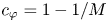 $c_\varphi =1-1/M$ (
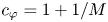 $c_\varphi =1+1/M$). In Mack's terminology, the first mode corresponds to an extension of the Tollmien–Schlichting mode, which is a viscous instability and originates from mode S in an eigenvalue spectrum. The second mode, which appears at hypersonic speeds, is rather inviscid and driven by acoustic waves. It is most often a continuation of mode S, but can also originate from mode F. The second synchronization occurs when mode F crosses the entropy/vorticity continuous branch. This corresponds to a sudden jump in the growth rate (as clearly visible in figure 1(c) of § 4.1). This discontinuity would not be present using DNS or parabolic stability equations (PSE), and is rather a mathematical artefact of the eigenvalue problem with Dirichlet free-stream boundary conditions. This results in the presence of continuous branches (Balakumar & Malik Reference Balakumar and Malik1992), and formally mode F corresponds to another eigenvalue after branch crossing. Fedorov & Tumin (Reference Fedorov and Tumin2011) show that a bi-orthogonal eigenvalue expansion (Tumin Reference Tumin2007, Reference Tumin2020), which includes, in addition to mode F, an infinite number of modes belonging to the continuous spectrum of LST, can resolve this inconsistency. Further downstream, a striking result of LST is that the maximum of amplification of the second mode (S or F) corresponds to a minimum of amplification for the other mode (F or S). During this opposite amplification, the wavenumbers and phase speeds (
 $c_\varphi$) of the two modes are almost equal, and the slope of
 $c_\varphi$ for mode S can exhibit an inflection to follow that of mode F (see figure 1b,d,f,h of § 4.1). This phenomenon, referred to as the FS synchronization, remains a mystery. Fedorov & Khokhlov (Reference Fedorov and Khokhlov2001) suggested an analytical model within the two-mode approximation, involving the sum of modes F and S with a particular branching dispersion relation. Taking into account the weakly non-parallel effects, they derived a rule for the intermodal exchange, explaining why mode S or F is unstable after the branching. An important conclusion from the discrete mode branching model is that the streamwise dependence of the base flow and of the amplitude function of the normal modes (eigenfunctions), which are neglected in a parallel theory, plays an important role for the intermodal exchange. It is worth noting that linear PSE (LPSE) calculations (Lifshitz, Degani & Tumin Reference Lifshitz, Degani and Tumin2012), which also take non-parallel effects into account, give a regular mode evolution in accordance with DNS results (Ma & Zhong Reference Ma and Zhong2003a). If discrete normal modes S and F are prescribed as inflow disturbances in LPSE, they evolve towards the same solution in the branching region, which correspond to the unstable mode F or S (see results of LPSE from Lifshitz et al. (Reference Lifshitz, Degani and Tumin2012) in figure 1e,g of § 4.1). It was concluded that LPSE or DNS do not exhibit a FS synchronization, and, due to mode coalescence, high streamwise gradients observed in the mode branching model of Fedorov & Khokhlov (Reference Fedorov and Khokhlov2001) are absent in LPSE. A conjecture made by Lifshitz et al. (Reference Lifshitz, Degani and Tumin2012) is that the second synchronization (F crossing the entropy/vorticity branch) can alter the FS synchronization because there is no longer a clear separation of the branching region from the continuous spectrum, and a complete model should include the continuous branch modes in addition to discrete F and S modes. Unfortunately, the eigenfunction expansion method is not applicable when branching of modes happens. It is thus not clear if the FS synchronization, not observed in LPSE and DNS, is the result of LST approximation rather than a physical feature. Nichols & Candler (Reference Nichols and Candler2019) used an input–output optimization to maximize the growth of second mode for a cold-wall boundary layer at
 $M=6.5$. They found a substantial amplification gain when both modes S and F are introduced at the inflow. Their linearized Navier–Stokes simulations thus show a coupling phenomenon, which could be associated with an FS synchronization.
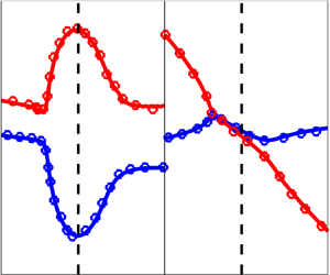
Phase speed as a function of  $Re$ at various Mach numbers: solid lines, present results; symbols, results from the literature (open symbols, LST from Ma & Zhong (Reference Ma and Zhong2003a) for
 $M=4.5$, and Fedorov & Tumin (Reference Fedorov and Tumin2011) for
 $M=5.5$ and
 $M=6.5$; filled symbols, PSE from Lifshitz et al. (Reference Lifshitz, Degani and Tumin2012) for
 $M=5.5$ and
 $M=6.5$). (a,c,e,g)
 $c_i$ (growth rate); (b,d,f,h)
 $c_r$. The adiabatic wall results are displayed in (a,b) (
 $M=4.5$) and (c,d) (
 $M=6$); (e,f) (
 $M=5.5$) and (g,h) (
 $M=6.5$) refer to the cold-wall cases. The solid vertical lines denote the location of the so-called FS synchronization.

Ma & Zhong (Reference Ma and Zhong2003a,Reference Ma and Zhongb) found that synchronization location and wave energy transfer play an important role in receptivity mechanisms. Though mode F (or mode S) may be linearly stable, it can have resonant interactions (synchronization) with both acoustic waves and the unstable mode S (or mode F). Zhu et al. (Reference Zhu, Zhang, Chen, Yuan, Wu, Chen, Lee and Gad-el Hak2016) and Chen, Zhu & Lee (Reference Chen, Zhu and Lee2017) also observed that modal interactions, between the second mode and the first mode, Görtler instabilities, or low-frequency content, have a catalytic impact on second-mode transition to turbulence.
1.3. Scope of the study
The primary goal of the study is to shed some light on the physical energy transfer mechanisms and the role of the initially unstable mode (either slow or fast) at hypersonic Mach number and for both adiabatic and cold-wall thermal conditions. For the analysis focusing on the early stages of laminar-to-turbulent transition, we develop a weakly nonlinear formulation following the work of Chu & Kovasznay (Reference Chu and Kovasznay1958). To account for non-parallel effects that were shown to be important by Fedorov & Khokhlov (Reference Fedorov and Khokhlov2001) for the intermodal exchange between slow and fast modes, the formulation accounts for non-parallel effects by considering the boundary-layer growth and the corresponding streamwise derivatives. The compressible Navier–Stokes equations are briefly recalled in § 2. The second-order nonlinear disturbance equations are developed in § 3 and the stability analysis is discussed in § 4 for various Mach numbers. In an attempt to understand the role played by the energy transfer mechanisms, both reversible and irreversible, between the perturbation kinetic energy ( $k$) and the temperature perturbation energy (
 $k_T$), in § 5 we develop the governing equations for the perturbation energies and for the perturbation entropy. Results are discussed in § 6, and conclusions of the study are given in § 7.
2. Governing equations
The conservation equations for high-Mach-number flows are written in Cartesian coordinates assuming a perfect gas and neglecting high-temperature effects. In divergence form they are
 $$\begin{gather} \frac{\partial\rho}{\partial t}+\frac{\partial J_j}{\partial x_j} = 0, \end{gather}$$
 $$\begin{gather}\frac{\partial(\rho u_i)}{\partial t}+\frac{\partial(J_j u_i)}{\partial x_j} ={-}\frac{\partial p}{\partial x_i } + \frac{\partial \sigma_{ij}}{\partial x_j}, \end{gather}$$
 $$\begin{gather}\frac{\partial(\rho T)}{\partial t}+\frac{\partial(J_j T)}{\partial x_j} ={-}\frac{p}{c_v} \frac{\partial u_j}{\partial x_j }+ \frac{\gamma}{Pr} \frac{\partial}{\partial x_j }\left(\mu \frac{\partial T}{\partial x_j}\right)+ \frac{1}{c_v} \rho\phi, \end{gather}$$
 $$\begin{gather}p =\rho R T , \end{gather}$$
where  $R$ is the gas constant and
 $\gamma =1.4$ is the ratio of the specific heat coefficients at constant pressure (
 $c_p$) and constant volume (
 $c_v$);
 $J_j$,
 $\sigma _{ij}$ and
 $\phi$ stand, respectively, for the
 $j$th convective flux component, the components of the stress tensor and the viscous dissipation:
 $$\begin{gather} J_j=\rho u_j, \end{gather}$$
 $$\begin{gather}\sigma_{ij}=\mu \left(2S_{ij}-\frac{2}{3}S_{\ell\ell}\delta_{ij}\right), \end{gather}$$
 $$\begin{gather}S_{ij}=\frac{1}{2}\left(\frac{\partial u_i}{\partial x_j}+\frac{\partial u_j}{\partial x_i}\right), \end{gather}$$
 $$\begin{gather}\phi=\frac{1}{ \rho}\sigma_{ij} S_{ij}, \end{gather}$$
 $S_{ij}$ being the symmetric strain tensor component and
 $\delta _{ij}$ the Kronecker delta. Sutherland's law is used for the viscosity
 $\mu$ and a constant Prandtl number
 $Pr=0.72$ is assumed.
3. Second-order nonlinear disturbance equations
Linear stability analysis relies on the assumption that for a generic disturbance, the flow variables can be decomposed in a basic state plus a disturbance, where the former is assumed to be a steady-state solution of the conservation equations. Substituting such a decomposition into the governing equations leads to a linearized set of equations that describe the evolution of the disturbances. By such an approach the fundamental physical mechanisms of stability in the very early stages of disturbance evolution have been elucidated. However, because of the founding assumption that disturbances are linearly independent, the interactions between disturbances cannot be considered. This is a major drawback, since disturbance interactions are responsible for nonlinear energy transfer mechanisms and for disturbance growth leading to turbulence transition. In the present study, we introduce a decomposition of the flow variables up to second order and account for the interactions between first- and second-order perturbations by developing a weakly nonlinear analysis following the work of Chu & Kovasznay (Reference Chu and Kovasznay1958).
Let  $q$ stand for either the velocity or the temperature, its instantaneous governing equation being cast in the form
 \begin{equation} \frac{\partial(\rho q)}{\partial t}+\frac{\partial(J_j q)}{\partial x_j}=R_q, \end{equation}
where, for brevity,  $R_q$ stands for the right-hand-side operator, whose expression is readily obtained from (2.1b)–(2.1c) and (2.2b)–(2.2d).
The weakly nonlinear governing equations are derived by introducing the following decomposition:
 \begin{equation} q=\bar{q} +\epsilon q^{\prime}+\epsilon^2 q^{\prime\prime}, \end{equation}
where  $\bar {q}$,
 $q^{\prime }$ and
 $q^{\prime \prime }$ represent, respectively, the base flow value and the first- and second-order disturbances of any variable
 $q$, and
 $\epsilon$ is a small positive number.
Substituting (3.2) in (3.1) and combining terms of the same order, the governing equations for the base flow (that are given in Appendix A) and for the first- and second-order disturbances are obtained.
3.1. Governing equations for first-order disturbances
The non-divergence form of the governing equations for the first-order disturbances  $q^{\prime }$ is obtained by combining the following equations:
 $$\begin{gather} \frac{\partial {\bar \rho}}{\partial t}+\frac{\partial{\bar J_j}}{\partial x_j} = 0, \end{gather}$$
 $$\begin{gather}\frac{\partial {\rho}^{\prime}}{\partial t}+\frac{\partial J_j^{\prime}}{\partial x_j} = 0, \end{gather}$$
 $$\begin{gather}\frac{\partial }{\partial t}({\bar \rho}{q^{\prime}}+ {\rho}^{\prime}{\bar q})+\frac{\partial}{\partial x_j} ( {\bar J_j}{q^{\prime}} + {J_j^{\prime}} {\bar q}) = R_q^{\prime}, \end{gather}$$
thus yielding
 \begin{equation} {\bar \rho}\frac{\partial q^{\prime}}{\partial t}+ {\bar J_j} \frac{\partial q^{\prime}}{\partial x_j}= R_q^{\prime}-{J_j^{\prime}}\frac{\partial \bar q}{\partial x_j}, \end{equation}
where  $\bar J_j$,
 $J_j^{\prime }$ and
 $R_q^{\prime }$ are, respectively, the base flow convective flux component, the first-order convective flux component and the first-order right-hand-side operator defined as
 $$\begin{gather} {\bar J}_j ={\bar \rho}{\bar u_j}, \end{gather}$$
 $$\begin{gather}J_j^{\prime} ={\rho}^{\prime}{\bar u_j}+{\bar \rho}u^\prime_j, \end{gather}$$
 $$\begin{gather}R_q^{\prime} =R_{q^{\prime}}={R_q}({\bar q},{\bar \rho},\ldots;q^{\prime},\rho^{\prime}\cdots). \end{gather}$$
3.2. Governing equations for second-order disturbances
The governing equations for the second-order disturbances are derived following the same procedure. In non-divergence form, the equation for the generic second-order disturbance  $q^{\prime \prime }$ is readily obtained by combining the base flow, first- and second-order continuity equations and the conservation equation for
 $q^{\prime \prime }$:
 $$\begin{gather} \frac{\partial {\bar \rho}}{\partial t}+\frac{\partial{\bar J_j}}{\partial x_j} = 0, \end{gather}$$
 $$\begin{gather}\frac{\partial {\rho}^{\prime}}{\partial t}+\frac{\partial J_j^{\prime}}{\partial x_j} = 0, \end{gather}$$
 $$\begin{gather}\frac{\partial {\rho}^{\prime\prime}}{\partial t}+\frac{\partial {J_j}^{\prime\prime}}{\partial x_j} ={-}\frac{\partial( {\rho}^{\prime} u^{\prime}_j)}{\partial x_j}, \end{gather}$$
 $$\begin{gather}\frac{\partial }{\partial t}({\bar \rho}{q^{\prime\prime}}+ {\rho}^{\prime\prime}{\bar q})+\frac{\partial}{\partial x_j} ( {\bar J_j}{q^{\prime\prime}} + {J_j^{\prime\prime}} {\bar q}) = R_q^{\prime\prime}-\frac{\partial( {\rho}^{\prime} {q^{\prime}}_j)}{\partial t}-\frac{\partial}{\partial x_j}( {\rho}^{\prime} u^{\prime}_j{\bar q}+J_j^{\prime}{q^{\prime}}), \end{gather}$$
thus obtaining
 \begin{equation} {\bar \rho}\frac{\partial q^{\prime\prime}}{\partial t}+ {\bar J_j} \frac{\partial q^{\prime\prime}}{\partial x_j}= R_q^{\prime\prime}-{J_j^{\prime\prime}} \frac{\partial \bar q}{\partial x_j}+{\bar \rho}N_{B,q}^{\prime\prime}, \end{equation}
where  $J_j^{\prime \prime }$ and
 $R_q^{\prime \prime }$ stand, respectively, for the second-order convective flux component and the second-order right-hand-side operator,
 $$\begin{gather} J_j^{\prime\prime} ={\rho}^{\prime\prime}{\bar u_j}+{\bar \rho}{u^{\prime\prime}_j}, \end{gather}$$
 $$\begin{gather}R_q^{\prime\prime} ={R_q}({\bar q},{\bar \rho},{\bar u_j}\cdots;q^{\prime\prime},\rho^{\prime\prime},u_j^{\prime\prime}\cdots;q^{\prime} \rho^{\prime},q^{\prime}u_j^{\prime},\rho^{\prime}u_j^{\prime}\cdots), \end{gather}$$
and  $N_{B,q}^{\prime \prime }$ accounts for the ‘bulk’ interactions of first-order disturbances driven by base flow gradients,
 \begin{equation} N_{B,q}^{\prime\prime}={-}\frac{\rho^{\prime}}{\bar \rho}\frac{\partial {q^{\prime}}}{\partial t}-\frac{J_j^{\prime}}{\bar \rho} \frac{\partial {q^{\prime}}}{\partial x_j} - \frac{\rho^{\prime}}{\bar \rho} u^{\prime}_j\frac{\partial {\bar q}}{\partial x_j}. \end{equation}
In order to derive a form-invariant formulation of the problem, the right-hand-side second-order term  $R_q^{\prime \prime }$ is recast as
 \begin{equation} R_q^{\prime\prime}=R_{q^{\prime\prime}}+N_{S,q}^{\prime\prime} , \end{equation}
where  $R_{q^{\prime \prime }}$ is only a function of the base flow properties and of the second-order disturbances, and has the same form as
 $R_q^{\prime }$:
 \begin{equation} R_{q^{\prime\prime}} ={R_q}({\bar q},{\bar \rho},{\bar u_j}\cdots;q^{\prime\prime}, \rho^{\prime\prime},u_j^{\prime\prime}\cdots). \end{equation}
Substituting (3.10) into (3.7) gives
 \begin{equation} {\bar \rho}\frac{\partial q^{\prime\prime}}{\partial t}+ {\bar J_j} \frac{\partial q^{\prime\prime}}{\partial x_j}= R_{q^{\prime\prime}}-{J_j^{\prime\prime}} \frac{\partial \bar q}{\partial x_j}+N_{B,q}^{\prime\prime}+N_{S,q}^{\prime\prime}. \end{equation}
For the velocity perturbations,  $N_{S,u_i}^{\prime \prime }=0$, whereas for the temperature perturbations,
 $N_{S,T}^{\prime \prime }$ represents an additional contribution due to viscous effects and thermal power dissipation (whose expression is given in the next section).
3.3. Disturbance governing equations
From the above analysis, the conservation equations for the  $n$th-order disturbances are then cast in the following form-invariant expression:
 \begin{align} &\qquad\quad\frac{\partial
\rho^{(n)}}{\partial t}+ \bar u_j\frac{\partial
\rho^{(n)}}{\partial x_j} + \bar \rho\frac{\partial
u_j^{(n)}}{\partial x_j} + u_j^{(n)}\frac{\partial \bar
\rho}{\partial x_j} + \rho^{(n)}\frac{\partial \bar
u_j}{\partial x_j} =
(n-1)N_{B,\rho}^{(n)},\end{align}
 \begin{align} & \frac{\partial u_i^{(n)}}{\partial t}+\bar u_j \frac{\partial u_i^{(n)}}{\partial x_j} +\frac{1}{\bar \rho}\frac{\partial p^{(n)}}{\partial x_i } -{\bar \nu} \frac{\partial}{\partial x_j}\left(2S_{ij}^{(n)}-\frac{2}{3}S_{\ell\ell}^{(n)}{\delta_{ij}}\right) -\frac{1}{\bar \rho}\left(2S_{ij}^{(n)}-\frac{2}{3}S_{\ell\ell}^{(n)}{\delta_{ij}}\right)\frac{\partial {\bar \mu}}{\partial x_j} \nonumber\\ &\quad +\frac{1}{\bar \rho}({\rho}^{(n)}{\bar u_j}+{\bar \rho}{u_j^{(n)}})\frac{\partial {\bar u_i}}{\partial x_j }= (n-1)N_{B,u_i}^{(n)}, \end{align}
 \begin{align} &\qquad\qquad
\frac{\partial T^{(n)}}{\partial t}+\bar u_j \frac{\partial
T^{(n)}}{\partial x_j} +\frac{1}{c_v} (p \theta)^{(n)}_L
-\frac{1}{\bar \rho}\frac{\gamma}{Pr}
\frac{\partial}{\partial x_j}\left({\bar \mu}
\frac{\partial T^{(n)}}{\partial x_j}\right)
-\frac{1}{c_v}{\phi^{(n)}_L} \nonumber\\ &\qquad\qquad\quad
+\frac{1}{\bar \rho}({\rho^{(n)}}{\bar u_j}+{\bar
\rho}u^{(n)}_j)\frac{\partial {\bar T}}{\partial x_j }=
(n-1)N_{B,T}^{(n)}+(n-1)N_{S,T}^{(n)},
\end{align}
 \begin{align}&\qquad\qquad\qquad\qquad p^{(n)} =R({\rho}^{(n)}{\bar T}+{\bar \rho}{T^{(n)}})+(n-1)N_{B,p}^{(n)}, \end{align}
where  $n=1,2$ and
 $(\cdot )^{(n)}$ is here used to indicate the
 $n$th-order perturbation of any variable
 $(\cdot )$, and
 \begin{equation} (p \theta)^{(n)}_L=\left( p^{(n)}\frac{\partial {\bar u}_i}{\partial x_i }+\bar p \frac{\partial u^{(n)}_i}{\partial x_i } \right) \quad \text{and} \quad {\phi^{(n)}_L}={\bar \nu}\left(4 {{\bar S}_{ij}}{S^{(n)}_{ij}}-\frac{4}{3}{\bar S}_{\ell\ell}S^{(n)}_{kk}\right) \end{equation}
are the  $n$th-order linearized pressure–dilatation and the linearized viscous dissipation. In the sections that follow we use
 $N_{q}^{(n)}=N_{B,q}^{(n)}+N_{S,q}^{(n)}$. For
 $n=1$,
 $N_{B,\rho }^{(1)}=0$,
 $N_{B,u_i}^{(1)}=0$,
 $N_{B,T}^{(1)}=0$ and
 $N_{B,p}^{(1)}=0$. For
 $n=2$,
 $$\begin{gather} N_{B,\rho}^{(2)}={-}\frac{\partial \rho^{(1)} u_j^{(1)}}{\partial x_j }, \end{gather}$$
 $$\begin{gather}N_{B,u_i}^{(2)}={-}\frac{\rho^{(1)}}{\bar \rho}\frac{\partial u_i^{(1)}}{\partial t }- \frac{1}{\bar \rho}({\rho}^{(1)}{\bar u_j}+{\bar \rho}{u_j^{(1)}})\frac{\partial u_i^{(1)}}{\partial x_j } -\frac{\rho^{(1)}}{\bar \rho}u_j^{(1)}\frac{\partial {\bar u_i}}{\partial x_j }, \end{gather}$$
 $$\begin{gather}N_{B,T}^{(2)}={-}\frac{\rho^{(1)}}{\bar \rho}\frac{\partial T^{(1)}}{\partial t }- \frac{1}{\bar \rho}({\rho}^{(1)}{\bar u_j}+{\bar \rho}{u_j^{(1)}})\frac{\partial T^{(1)}}{\partial x_j } -\frac{\rho^{(1)}}{\bar \rho}u_j^{(1)}\frac{\partial {\bar T}}{\partial x_j }, \end{gather}$$
 $$\begin{gather}N_{B,p}^{(2)}=R\rho^{(1)}T^{(1)}, \end{gather}$$
 $$\begin{gather}N_{S,T}^{(2)}={-}\frac{1}{{\bar \rho}c_v} p^{(1)}\frac{\partial u_j^{(1)}}{\partial x_j } +\frac{\bar \nu}{c_v}\left( 2S_{ij}^{(1)}S_{ij}^{(1)}-\frac{2}{3}S_{\ell\ell}^{(1)}S_{kk}^{(1)}\right). \end{gather}$$
The governing equations for first- and second-order disturbances in Cartesian coordinates are given in supplementary material available at https://doi.org/10.1017/jfm.2024.912.
4. Stability analysis to second order
To account for the interactions between disturbances in the early phase of their evolution, the above equations are solved for both the first- and second-order disturbances.
In a compact form, the transport equations of the first-order disturbances (3.13a)–(3.13d) are cast in the form
 \begin{equation} {\mathcal{L}}(x,y,z,t;\bar \rho, \bar u ,\ldots; \rho^{\prime},u^{\prime},v^{\prime}, w^{\prime},p^{\prime},T^{\prime} )=0, \end{equation}
where  $\mathcal {L}$ is the linearized compressible Navier–Stokes equations for the first-order disturbances and that has been derived in the previous section.
First-order disturbances are obtained by solving (4.1) for two-dimensional normal-form disturbances, yielding a generalized eigenvalue problem, whose solution gives a set of linearly independent eigenmodes  $\hat{\boldsymbol{q}}'(y)$ (hereafter also referred to as modes) and the complex streamwise wavenumber
 $\alpha$ for a given angular frequency
 $\omega$. The stability equations are solved in dimensionless form, where variables are made non-dimensional with respect to the free-stream values (
 $\rho _{\infty },u_{\infty },\rho _{\infty } u_{\infty }^2,T_{\infty })$ and the Blasius length
 $\ell$ is used as reference length scale such that
 \begin{equation} Re=\frac{\rho_{\infty} u_{\infty} \ell}{\mu_{\infty}}=\sqrt{\frac{\rho_{\infty} u_{\infty} x}{\mu_{\infty}}}=\sqrt{Re_x}. \end{equation}
The non-dimensional frequencies are then given as
 \begin{equation} \omega= \frac{\omega^* \ell}{u_{\infty}} \quad \text{and} \quad F=\frac{\omega^* \mu_{\infty}}{\rho_{\infty} {u_{\infty}}^2}, \end{equation}
where  $\omega = Re F$ is the non-dimensional circular frequency.
For the transport equations of the second-order disturbances, we exploit the form-invariance form of (3.13a)–(3.13d) that are cast in the following compact form:
 \begin{equation} {\mathcal{L}}(x,y,z,t;\bar \rho, \bar u ,\ldots; \rho^{\prime\prime},u^{\prime\prime}, v^{\prime\prime},w^{\prime\prime},p^{\prime\prime},T^{\prime\prime} )= {\mathcal{N}}(\bar \rho, \bar u ,\ldots; \rho^{\prime}u^{\prime},\rho^{\prime}v^{\prime},\ldots), \end{equation}
where  ${\mathcal {N}}=[N_{B,\rho },N_{B,u_i},N_{B,T}+N_{S,T}]$ represents the (weakly) nonlinear terms that drive the evolution of the second-order modes, which are assumed to have the normal form
 \begin{equation} \boldsymbol{q}^{\prime\prime}={\hat{\boldsymbol{q}}}^{\prime\prime}(y)\exp\left({{\rm i}\left(\int_{}^{x} \alpha \,{{\rm d}\kern 0.06em x}-\omega t\right)}\right). \end{equation}
Introducing the normal-mode expansion of the disturbances, a single set of equations is written for the first- and second-order modes ( ${\hat{\boldsymbol{q}}}^{\prime }$ and
 ${\hat{\boldsymbol{q}}}^{\prime \prime }$). Assuming a two-dimensional non-parallel flow with the base flow assumed to vary in both the streamwise and wall-normal directions, namely
 ${\bar u}={\bar u}(x,y), {\bar v}={\bar v}(x,y),{\bar w}=0, {\bar \rho }={\bar \rho }(x,y), {\bar T}={\bar T}(x,y), {\bar p}={\bar p}(x,y)$, the stability equations for the first- and second-order modes are recovered. In a compact matrix form, the stability equations are cast as
 \begin{equation}
\boldsymbol{\mathsf{C}}\frac{{\rm d}^2 \hat{\boldsymbol{q}}}{{{\rm d}y}^2}+\boldsymbol{\mathsf{B}}\frac{{\rm d} \hat{\boldsymbol{q}}}{{{\rm d}y}}+\boldsymbol{\mathsf{A}}{\hat{\boldsymbol{q}}}=(n-1) f {\skew2\hat{\boldsymbol{\mathsf{N}}}}, \end{equation}
where  $\boldsymbol{\mathsf{A}}=\boldsymbol{\mathsf{A}}(\alpha,\omega,M,Re; {\bar \rho },{\bar u_i},{\bar p},{\bar T})$,
 $\boldsymbol{\mathsf{B}}=\boldsymbol{\mathsf{B}}(\alpha,\omega,M,Re; {\bar \rho },{\bar u_i},{\bar p},{\bar T})$ and
 $\boldsymbol{\mathsf{C}}=\boldsymbol{\mathsf{C}}(\alpha,\omega, M,Re; {\bar \rho },{\bar u_i},{\bar p},{\bar T})$ are (
 $5 \times 5$) matrices whose expressions are given in Appendix B;
 ${\hat {\boldsymbol{\mathsf{N}}}}$ is the normal-mode representation of the first-order mode interaction contribution to the second-order ones. The density mode and its
 $x$ and
 $y$ derivatives are determined from the linearized equation of state. Note that the viscosity disturbances (
 $({{\rm d} \bar \mu }/{{\rm d} T}){\hat T^{\prime }}$ and
 $({{\rm d} \bar \mu }/{{\rm d} T}){\hat T^{\prime \prime }}$, respectively) have been found not to affect the stability (for brevity, results of the analysis are not reported) and have been neglected. The factor
 $f=\exp ({{\rm i}(\int _{}^{x} \alpha \,{{\rm d}\kern 0.06em x} -\omega _0 T_0/2)}) \sin ({\omega _0 T_0}/2)/({\omega _0 T_0}/2)$ accounts for cycle-averaged nonlinear effects (Kuehl Reference Kuehl2018), where
 $\omega _0$ and
 $T_0$ are, respectively, the angular frequency and the corresponding period at synchronization location
 $T_0=\ell _0/u_{\infty }$ (
 $\ell _0$ being the Blasius length at synchronization). In practice, a first LST calculation is performed to determine the synchronization frequency corresponding to the maximum amplification of the unstable mode, which provides the reference Blasius length
 $\ell _0$ to form the reference Reynolds number
 $Re_0$ for LST computations. In the following, the results are presented using the local Reynolds number
 $Re$ and the dimensionless phase speed
 $c_{\varphi }=\omega /\alpha =c_r+i c_i$ is used, as suggested by Lifshitz et al. (Reference Lifshitz, Degani and Tumin2012), since its value does not depend on the length scale
 $\ell _0$ (contrary to the complex wavenumber that does depend on
 $\ell _0$). To account for the thickening of the boundary layer, the base flow equations are solved in the transformed space (
 $x, y/\delta (x)$), and
 $\ell _0$ and the corresponding Reynolds number
 $Re_0$ are chosen as reference.
For  $n=1$, (B1) reduces to the linear stability equation
 \begin{equation} {\hat{\boldsymbol{\mathsf{L}}}}{\hat{\boldsymbol{q}}}^{\prime}= 0, \end{equation}
where
 \begin{equation}
{\hat{\boldsymbol{\mathsf{L}}}}=\boldsymbol{\mathsf{C}}\frac{{\rm d}^2 }{{{\rm d}y}^2}+\boldsymbol{\mathsf{B}}\frac{{\rm d}}{{{\rm
d}y}}+\boldsymbol{\mathsf{A}}={\hat{\boldsymbol{\mathsf{L}}}} (\alpha,\omega,M,Re; {\bar \rho},{\bar
u_i},{\bar p},{\bar T}),
\end{equation}
with homogeneous boundary conditions. Namely,  ${\hat u^{\prime }}={\hat v^{\prime }}={\hat w^{\prime }}=0$ and
 ${{\rm d} \hat p^{\prime }}/{{\rm d}y}=0$, both at the wall and at free stream, and
 ${\hat T^{\prime }}=0$ at the wall and
 ${{\rm d}\hat T^{\prime }}/{{\rm d}y}=0$ at free stream.
Equation (4.7) constitutes an eigenvalue problem in the wavenumber  $\alpha$ that depends on the Mach and Reynolds numbers. The discretized eigenproblem is transformed into a problem with linear eigenvalues, and solved with the shift-invert method and a QZ algorithm and taking
 $\bar v=0$. A Newton–Raphson algorithm is implemented to follow the selected modes (see Gloerfelt & Robinet (Reference Gloerfelt and Robinet2017) for more details).
For  $n=2$, the second-order stability equation is
 \begin{equation} {\hat{\boldsymbol{\mathsf{L}}}}{\hat{\boldsymbol{q}}}^{\prime\prime}= f {\skew2\hat{\boldsymbol{\mathsf{N}}}}. \end{equation}
The second-order modes are then computed from the relation
 \begin{equation} {\hat{\boldsymbol{q}}}^{\prime\prime}= f {\hat{\boldsymbol{\mathsf{L}}}}^{{-}1}{\skew2\hat{\boldsymbol{\mathsf{N}}}}. \end{equation}
To second order, the disturbance mode of any variable  $q$ is then computed as the sum of the first- and second-order modes (
 $\epsilon {\hat{\boldsymbol{q}}}^{\prime }+\epsilon ^2{\hat{\boldsymbol{q}}}^{\prime \prime }$).
4.1. Linear stability results
The influence of the Mach number and of the wall thermal state is here analysed considering both adiabatic and cold-wall conditions (see table 1). In the table we also report the values of the Mach numbers and the corresponding values of the boundary-layer thickness ( $\delta _0$), the generalized inflection point distance (
 $y_{gip}$), the sonic line
 $y$ position (
 $y_{s,S}$ and
 $y_{s,F}$ of the slow and fast modes, respectively) and the critical layer height (
 $y_{c,S}$ and
 $y_{c,F}$) at synchronization location (i.e. at the reference streamwise location), where
 $y_{gip}$ is defined as
 ${\partial }/{\partial y}(\bar \rho {\partial \bar u}/{\partial y})=0$. The selected conditions of the adiabatic wall cases are those of Ma & Zhong (Reference Ma and Zhong2003a) and Reed & Balakumar (Reference Reed and Balakumar1990) for
 $M=4.5$ and
 $M=6$, respectively, whereas for the cold-wall cases they are those of Fedorov & Tumin (Reference Fedorov and Tumin2011). For the former, the selected non-dimensional frequency is
 $F=2.2\times 10^{-4}$; for the cold-wall cases the selected value of
 $F$ is
 $1 \times 10^{-4}$. All selected cases are inviscidly unstable. As expected, the generalized inflection point moves farther away from the wall as the Mach number increases, with the exception of the
 $M=5.5$ case that presents an inflection point at the wall.
Base flow boundary-layer parameters (thickness, generalized inflection point, sonic line and critical layer heights) for various Mach numbers.

For comparison with the literature, all results are presented in terms of the local Reynolds number (4.2), the growth rate being represented in terms of the imaginary part of the phase speed  $c_i$ (Lifshitz et al. Reference Lifshitz, Degani and Tumin2012). Figure 1 showcases the real and imaginary parts of the phase speeds that are in very good agreement with the literature (symbols in figure 1). Note that the vertical dashed lines in the figure identify the analysed domain around synchronization location. The slow mode of the adiabatic (
 $M=4.5$ and
 $M=6$) and cold (
 $M=6.5$) wall cases is initially unstable, whereas for
 $M=5.5$ the fast mode is initially unstable. The unstable mode (slow or fast) reaches its maximum amplification as the other mode (fast or slow) attains a minimum. The phase velocity of the two modes is then very close, and this phenomenon is called synchronization. Past synchronization location, mode S of the two adiabatic cases and of the cold case at
 $M=5.5$ exhibits a slightly increasing Mach number (relative to the phase speed) still remaining subsonic, whereas mode F shows a continuously decreasing phase speed. An opposite behaviour is observed for case
 $M=6.5$, namely the phase speed of the fast mode has a tendency to increase whereas it continuously decreases for mode S.
The wall-normal distributions of the eigenfunction amplitudes and phases at synchronization location are reported in figure 2 for the slow and the fast modes, respectively. The amplitudes are normalized by the pressure amplitude at the wall. The behaviour of the adiabatic (respectively, cold) wall cases being similar, unless significant differences occur, hereafter we only report the results for  $M=4.5$ and
 $M=5.5$. The figure shows that the eigenfunctions are dominated by the fluctuations in thermodynamic variables. In the subsonic layer, pressure, temperature and streamwise velocity perturbations are approximately in phase and in nearly phase opposition with the wall-normal velocity. It is also interesting to observe that for the cold wall the reduction of the boundary-layer scales affects the initially unstable mode that experiences a smaller peak in the temperature perturbation amplitude at the critical layer. The phase behaviour is overall less affected by the wall thermal conditions.
Eigenfunction amplitudes and phases at synchronization location for (a) adiabatic wall ( $M=4.5$) and (b) cold wall (
 $M=5.5$). Solid lines, initially unstable mode; dashed lines, initially stable mode.

4.2. Budget analysis
To identify the dominant physical mechanisms and to elucidate their role in the slow and fast modes, we have scrutinized the budgets of the various perturbation variables at synchronization location. In the following, we report the budgets of the streamwise and wall-normal velocity and temperature disturbances that are discussed in detail in the discussion section.
For the analysis, the total time rate of change of any variable  $\widehat {(\cdot )}$ is split in two terms, namely
 $({\hat {\rm D}}/{{\rm D} t}) \widehat {(\cdot )}={\rm i}(\alpha {\bar u}-\omega ) \widehat {(\cdot )}$ (which accounts for the streamwise contribution) and
 ${\bar v} ({d \widehat {(\cdot )}}/{{\rm d}y})$ that represents the (convective) transport due to base flow wall-normal velocity component.
Dropping superscripts  $(\hat {\cdot })^{\prime }$ and
 $(\hat {\cdot })^{\prime \prime }$, the normal-mode expression of the budget equation for the streamwise velocity disturbance (of either first or second order) is cast in the form
 \begin{equation} \frac{\hat {\rm D} \hat u}{{\rm D} t}+\bar v \frac{{\rm d} {\hat u}}{{{\rm d}y} }={-}{\rm i}\alpha \frac{\hat p}{\bar \rho}+D_u+\textit{u-mgP}+(n-1)f \hat N_u, \end{equation}
where
 \begin{gather} \frac{\hat {\rm D} \hat u}{{\rm D} t}={\rm i}\left(\alpha {\bar u}-\omega\right){\hat u}, \end{gather}
 \begin{gather}\begin{aligned}[b] D_u &= \frac{1}{\bar
\rho}\left\{ \left[\frac{4}{3}{\bar \mu}\left({\rm
i}\frac{{\rm d} \alpha}{{\rm d}\kern 0.06em x}-\alpha^2\right)+\frac{4}{3}{\rm i}\alpha\frac{\partial
\bar \mu}{\partial y}\right]{\hat u} +{\bar \mu}\frac{{\rm
d}^2 {\hat u}}{{{\rm d}y}^2 }+ \frac{\partial {\bar
\mu}}{\partial y }\frac{{\rm d} {\hat u}}{{{\rm
d}y}} \right.\nonumber\\ &\quad \left.+\,{\rm
i}\alpha\frac{\partial \bar \mu}{\partial y}{\hat
v}+\left({\rm i}\frac{1}{3}\alpha{\bar
\mu}-\frac{2}{3}\frac{\partial {\bar \mu}}{\partial x
}\right)\frac{{\rm d} {\hat v}}{{{\rm d}y}}\right\},\end{aligned}
\end{gather}
 $$\begin{gather} \textit{u-mgP}={-}\left[{\hat u}+{\bar u}\left(\frac{\hat p}{\bar p}-\frac{\hat T}{\bar T}\right)\right]\frac{\partial {\bar u}}{\partial x } -\left[{\hat v}+{\bar v}\left(\frac{\hat p}{\bar p}-\frac{\hat T}{\bar T}\right)\right]\frac{\partial {\bar u}}{\partial y }, \end{gather}$$
 $$\begin{gather}\hat N_u = \frac{1}{\bar \rho}\left[{\rm i}\omega{\hat \rho}^{\prime}{\hat u}^{\prime}-{\rm i}\alpha({\hat \rho}^{\prime} {\bar u}+{\bar \rho}{\hat u}^{\prime}){\hat u}^{\prime} -({\hat \rho}^{\prime} {\bar v}+{\bar \rho}{\hat v}^{\prime})\frac{{\rm d} {\hat u}^{\prime}}{{{\rm d}y} } -{\hat \rho}^{\prime}{\hat u}^{\prime}\frac{\partial {\bar u}}{\partial x }-{\hat \rho}^{\prime}{\hat v}^{\prime}\frac{\partial {\bar u}}{\partial y }\right], \end{gather}$$
where  $n=1$ for the budget of the first-order mode
 $(\hat {\cdot })^{\prime }$ and
 $n=2$ for the second-order mode
 $(\hat {\cdot })^{\prime \prime }$. The right-hand side of (4.11) represents the contributions due to the streamwise pressure gradient, diffusion, transport of streamwise momentum disturbances resulting from the base flow/perturbation interaction driven by the base flow velocity gradient and the contribution resulting from the interaction of first-order modes.
The budget equation for the wall-normal velocity disturbance is written as
 \begin{equation} \frac{\hat {\rm D} \hat v}{{\rm D} t}+\bar v \frac{{\rm d} \hat v}{{\rm d}y}={-}\frac{1}{\bar \rho} \frac{{\rm d} \hat p}{{\rm d}y}+D_v+\textit{v-mgP}+(n-1)f \hat N_v, \end{equation}
with  $n=1,2$, and where
 \begin{gather} \frac{\hat {\rm D} \hat v}{{\rm D} t}={\rm i}(\alpha {\bar u}-\omega){\hat v}, \end{gather}
 \begin{gather}\begin{aligned} D_v &=
\frac{1}{\bar \rho}\left\{ -\frac{2}{3}{\rm
i}\alpha\frac{\partial \bar \mu}{\partial y}{\hat
u}+\left({\rm i}\frac{1}{3}\alpha{\bar \mu}-\frac{\partial
{\bar \mu}}{\partial x }\right) \frac{{\rm d}{\hat
u}}{{{\rm d}y}} \right.\nonumber\\ &\quad\times
\left.\left[{\bar \mu}\left({\rm i}\frac{{\rm d}
\alpha}{{\rm d}\kern 0.06em x}-\alpha^2\right)+{\rm
i}\alpha\frac{\partial \bar \mu}{\partial x}\right]{\hat v}
+\frac{4}{3}\left({\bar \mu}\frac{{\rm d}^2 {\hat v}}{{{\rm
d}y}^2 }+ \frac{\partial {\bar \mu}}{\partial y }\frac{{\rm
d} {\hat v}}{{{\rm d}y} }\right) \right\},
\end{aligned}\end{gather}
 $$\begin{gather} \textit{v-mgP}={-}\left[{\hat u}+{\bar u}\left(\frac{\hat p}{\bar p}-\frac{\hat T}{\bar T}\right)\right]\frac{\partial {\bar v}}{\partial x } -\left[{\hat v}+{\bar v}\left(\frac{\hat p}{\bar p}-\frac{\hat T}{\bar T}\right)\right]\frac{\partial {\bar v}}{\partial y }, \end{gather}$$
 $$\begin{gather}\hat N_v = \frac{1}{\bar \rho}\left[{\rm i}\omega{\hat \rho}^{\prime}{\hat v}^{\prime}-{\rm i}\alpha({\hat \rho}^{\prime} {\bar u}+{\bar \rho}{\hat u}^{\prime}){\hat v}^{\prime} -\left({\hat \rho}^{\prime} {\bar v}+{\bar \rho}{\hat v}^{\prime}\right)\frac{{\rm d} {\hat v}^{\prime}}{{{\rm d}y} } -{\hat \rho}^{\prime}{\hat u}^{\prime}\frac{\partial {\bar v}}{\partial x }-{\hat \rho}^{\prime}{\hat v}^{\prime}\frac{\partial {\bar v}}{\partial y }\right]. \end{gather}$$
Similarly, the budget equation for the temperature disturbance  $\hat T = {\hat e}/c_v$ is written as
 \begin{equation} \frac{\hat {\rm D}{\hat T}}{{\rm D} t }+{\bar v} \frac{{\rm d} \hat T}{{\rm d}y} ={-} \frac{1}{\bar \rho c_v}(p \theta)_L + D_T + \frac{1}{c_v}{{\hat \phi}_L}+ {T\textit{-}mgP}+(n-1)f {\hat N}_{T} \end{equation}
( $n=1$, 2), where
 ${\hat {\rm D}{\hat T}}/{{\rm D} t}$,
 $(p \theta )_L$,
 $D_T$,
 ${{\hat \phi }_L}$,
 ${{\hat \phi }_{T,L}}$,
 ${T\textit {-}mgP}$ and
 ${\hat N}_{T}$ stand for, respectively, the total time rate of change of
 ${\hat T}$, the exchanges of internal energy due to (linearized) pressure–dilatation and heat conduction, the (linearized) viscous dissipation contribution, the (linearized) thermal power dissipation, the exchanges of internal energy disturbances resulting from base flow/perturbation interaction driven by base flow temperature gradients and the contribution resulting from first-order mode interactions, whose expressions are given in the following:
 $$\begin{gather} \frac{\hat {\rm D} \hat T}{{\rm D} t}={\rm i}(\alpha {\bar u}-\omega){\hat T}, \end{gather}$$
 $$\begin{gather}(p \theta)_L={-}{\bar p}\left({\rm i}\alpha{\hat u}+\frac{{\rm d} {\hat v}}{{{\rm d}y} }\right)-{\hat p}\left(\frac{\partial \bar u}{\partial x }+\frac{\partial \bar v}{\partial y}\right), \end{gather}$$
 $$\begin{gather}D_T=\frac{\gamma}{Pr} \frac{1}{\bar \rho}\left\{\left[{\bar \mu}\left(-\alpha^2+{\rm i}\frac{{\rm d} \alpha}{{\rm d}\kern 0.06em x}\right)+{\rm i}\alpha\frac{\partial {\bar \mu}}{\partial x }\right]{\hat T} +\left[{\bar \mu}\frac{{\rm d}^2 {\hat T}}{{{\rm d}y}^2 }+\frac{\partial \bar \mu}{\partial y }\frac{{\rm d} {\hat T}}{{{\rm d}y} }\right]\right\}, \end{gather}$$
 \begin{gather}\begin{aligned}[b] {{\hat \phi}_L} &={\bar
\nu} \left\{ 4 \left(\frac{\partial \bar u}{\partial x}
{\rm i} \alpha {\hat u} + \frac{\partial \bar v}{\partial
y}\frac{{\rm d} {\hat v}}{{\rm d}y}\right)
+2\left(\frac{\partial \bar u}{\partial y}+\frac{\partial
\bar v}{\partial x}\right)\left(\frac{{\rm d} {\hat
u}}{{\rm d}y}+{\rm i} \alpha {\hat v}\right)
\right.\nonumber\\ &\quad
\left.-\frac{4}{3}\left(\frac{\partial \bar u}{\partial
x}+\frac{\partial \bar v}{\partial y}\right)\left({\rm i}
\alpha {\hat u} + \frac{{\rm d} {\hat v}}{{\rm d}y}\right)
\right\},
\end{aligned}\end{gather}
 \begin{gather} \textit{T-mgP}={-}\left[{\hat u}+{\bar u}\left(\frac{\hat p}{\bar p}-\frac{\hat T}{\bar T}\right)\right]\frac{\partial {\bar T}}{\partial x } -\left[{\hat v}+{\bar v}\left(\frac{\hat p}{\bar p}-\frac{\hat T}{\bar T}\right)\right]\frac{\partial {\bar T}}{\partial y }, \end{gather}
 \begin{gather}\begin{aligned}[b] \hat N_T &= \frac{1}{\bar
\rho}\left\{ {\rm i}\omega{\hat \rho}^{\prime}{\hat
T}^{\prime}-{\rm i}a({\hat \rho}^{\prime} {\bar u}+{\bar
\rho}{\hat u}^{\prime}){\hat T}^{\prime} -({\hat
\rho}^{\prime} {\bar v}+{\bar \rho}{\hat
v}^{\prime})\frac{{\rm d} {\hat T}}{{{\rm d}y} } -{\hat
\rho}^{\prime}{\hat u}^{\prime}\frac{\partial {\bar
T}}{\partial x }-{\hat \rho}^{\prime}{\hat
v}^{\prime}\frac{\partial {\bar T}}{\partial y }
\right.\nonumber\\ &\quad -\frac{{1}}{c_v}{\hat
p}^{\prime}\left({\rm i}\alpha{\hat u}^{\prime}+\frac{{\rm
d} {\hat{v}^{\prime}}}{{{\rm d}y} }\right)+\frac{{\bar
\mu}}{c_v}\left[{-}2\alpha^2({\hat u}^{\prime})^2+2
\left(\frac{{\rm d} {\hat{v}^{\prime}}}{{{\rm
d}y}}\right)^2+ \left(\frac{{\rm d}
{\hat{u}^{\prime}}}{{{\rm d}y}}+{\rm
i}\alpha{\hat{v}^{\prime}}\right)^2 \right.\nonumber\\
&\quad \left.\left.-\,\alpha^2({\hat
w}^{\prime})^2+\left(\frac{{\rm d}
{\hat{w}^{\prime}}}{{{\rm d}y}}\right)^2
-\frac{2}{3}\left({\rm i}\alpha{\hat u}^{\prime}+\frac{{\rm
d} {\hat{v}^{\prime}}}{{{\rm d}y} }\right)^2\right]
+\left(\bar u\frac{\partial {\bar T}}{\partial x }+\bar v
\frac{\partial {\bar T}}{\partial y }\right){\hat
\rho}^{\prime} \frac{{\hat T}^{\prime}}{{\bar T}}\right\}.\end{aligned}
\end{gather}
To interpret and understand the physical mechanisms controlling the wall behaviour of the perturbations we have also analysed in detail the budgets in the near-wall proximity (i.e. in the limit  ${y \to 0}$). Taking into account the boundary conditions at the wall, namely
 ${\hat u} = {\hat v} = {\hat w} = {\hat T} = 0$ and
 ${\bar u} = {\bar v} = {\partial \bar p}/{\partial y }=0$, the normal-mode expression of the continuity equation (3.13a) and equations (4.11), (4.13) and (4.15) reduce to
 $$\begin{gather} \frac{{\rm d} {\hat v}}{{{\rm d}y} }= {\rm i} \omega \frac{{\hat p}}{\bar p}-\frac{\partial \bar v}{\partial y}\frac{{\hat p}}{\bar p} - (n-1)f \frac{{\hat p}^{\prime}}{\bar p} \frac{{\rm d} {\hat v}^{\prime}}{{{\rm d}y}}, \end{gather}$$
 $$\begin{gather}{\bar \mu}\frac{{\rm d}^2 {\hat u}}{{{\rm d}y}^2 }= {\rm i}\alpha{\hat p}+ \frac{2}{3}\frac{{\rm d} {\hat v}}{{{\rm d}y} }\frac{\partial {\bar \mu}}{\partial x } -\frac{{\rm d} {\hat u}}{{{\rm d}y} }\frac{\partial {\bar \mu}}{\partial y }, \end{gather}$$
 $$\begin{gather}\frac{4}{3}{\bar \mu}\frac{{\rm d}^2 {\hat v}}{{{\rm d}y}^2}=\frac{{\rm d} {\hat p}}{{{\rm d}y} }-\frac{4}{3}\frac{{\rm d} {\hat v}}{{{\rm d}y} }\frac{\partial {\bar \mu}}{\partial y } -\frac{{\rm d} {\hat u}}{{{\rm d}y} }\frac{\partial {\bar \mu}}{\partial x }, \end{gather}$$
 \begin{gather}\begin{aligned}[b] {\bar p}\frac{{\rm d} {\hat v}}{{{\rm d}y} } &= \frac{c_p}{Pr}\frac{{\rm d} }{{\rm d}y}\left({\bar \mu}\frac{{\rm d} {\hat T}}{{{\rm d}y} }\right) +\left[ \frac{8}{3}{\bar \mu}\frac{\partial {\bar v}} {\partial y }\frac{{\rm d} {\hat v}}{{{\rm d}y} } +2{\bar \mu}\frac{\partial {\bar u}} {\partial y }\frac{{\rm d} {\hat u}}{{{\rm d}y} } \right] -{\hat p}\frac{\partial {\bar v}} {\partial y } \nonumber\\ &\quad - (n-1)f\left({\hat p}^{\prime} \frac{{\rm d} {\hat v}^{\prime}}{{{\rm d}y} }-\bar \rho{\hat \phi}^{\prime}\right), \end{aligned}\end{gather}
where  ${\hat \phi }^{\prime }={\bar \nu }[\frac {4}{3}({{\rm d} {\hat {v}^{\prime }}}/{{{\rm d}y} })^2 +({{\rm d} {\hat {u}^{\prime }}}/{{{\rm d}y} })^2 +({{\rm d} {\hat {w}^{\prime }}}/{{{\rm d}y} })^2]$ and
 $n=1,2$.
4.2.1. The  $u$ budget

Figure 3 reports the amplitudes and phases of the various terms of the budgets of the slow and fast  ${\hat u}$ modes at synchronization location for adiabatic wall (
 $M=4.5$) and cold wall (
 $M=5.5$). At
 $M=4.5$,
 ${\hat D \hat u}/{{\rm D} t }$ is primarily driven by the streamwise pressure gradient and by the base flow/perturbation interaction term. The latter attains a maximum in the subsonic layer (at
 $y/\delta \approx 1/4$), whereas
 ${\hat {\rm D} \hat u}/{{\rm D} t }$ is maximum in the very near-wall region (
 $y/\delta \approx 1/10$). The figure also shows that the effect of u-mgP is stronger for cold wall than for adiabatic wall. It is worth noting that this one-way coupling term reflects the assumption that the base flow and the disturbances are weakly coupled. Namely, the reciprocal effect leading to base flow distortion is neglected. At the wall, as predicted from the asymptotic perturbation equation (4.17b), diffusion and streamwise pressure gradient are in equilibrium (namely, diffusion of the perturbation streamwise velocity is dictated by the streamwise pressure gradient).
Budgets of the streamwise velocity perturbation of modes S and F for (a) adiabatic wall ( $M=4.5$) and (b) cold wall (
 $M=5.5$). Modulus in the first row and phase in the second row.

For fast modes,  ${{\hat {\rm D}} {\hat u}}/{{\rm D} t }$,
 $-{\rm i}\alpha ({1}/{\bar \rho }){\hat p}$ and u-mgP are approximately in phase within the subsonic layer. For slow modes,
 ${{\hat {\rm D}} {\hat u}}/{{\rm D} t }$ and
 $-{\rm i}\alpha ({1}/{\bar \rho }){\hat p}$ are nearly in phase opposition in the vicinity of the critical layer (where
 ${\bar u}=c_r$). At the critical layer
 ${{\hat {\rm D}} {\hat u}}/{{\rm D} t }$ exhibits a phase jump. Note that no significant change in the behaviour is observed across synchronization (data not reported).
4.2.2. The $v$ budget

The budgets of the slow and fast  $\hat v$ modes are displayed in figure 4. The evolution of the wall-normal perturbation velocity mode
 $\hat v$ is essentially driven by the wall-normal pressure gradient. Its total time rate of change
 ${{\hat {\rm D}} {\hat v}}/{{\rm D} t}$ and
 $-({1}/{\bar \rho })({{\rm d} \hat p}/{{\rm d}y})$ superpose in both amplitude and phase, for both slow and fast modes and for all Mach numbers. At the wall, as in the case of the perturbation streamwise velocity, diffusion balances the perturbation wall-normal pressure gradient.
Budgets of the wall-normal velocity perturbation of modes S and F for (a) adiabatic wall ( $M=4.5$) and (b) cold wall (
 $M=5.5$).

The streamwise distributions of the amplitude and phase of the wall perturbation–dilatation  $\theta ={{\rm d} {\hat v}}/{{{\rm d}y}}$, the (negative) time rate of change of the pressure perturbation
 ${\rm i} \omega ({\hat p}/{\bar p})$ and the (negative) mean dilatation term
 $-({\hat p}/{\bar p}){\bar \theta }$ (
 ${\bar \theta }={\partial \bar v}/{\partial y})$ around synchronization are reported in figure 5 for both the S and F modes. The figure shows that, in the near-wall proximity, the effect of the mean dilatation is negligible and
 ${{\rm d} {\hat v}}/{{{\rm d}y}}\approx {\rm i} \omega ({\hat p}/{\bar p})$; namely, the wall perturbation–dilatation is driven by the time rate of change of pressure perturbation with a phase lag of approximately
 $90^{\circ }$ independently of the Mach number.
Streamwise distribution of wall dilatation of modes S and F for (a) adiabatic wall ( $M=4.5$) and (b) cold wall (
 $M=5.5$). Upper panels, amplitude; lower panels, phase.

4.2.3. The $T$ budget

For adiabatic wall, the budgets of the slow and fast  $\hat T$ modes (figure 6) show that, in the subsonic layer,
 ${{\hat {\rm D}} {\hat T}}/{{\rm D} t}$ is primarily driven by the (linearized) pressure–dilatation
 $(p \theta )_L$. In the supersonic region, in addition to heat conduction effects (whose contribution is most significant in the proximity of the critical layer), the exchanges of internal energy associated with the perturbation/base flow interaction (T-mgP) also play a role. For cold wall, in the subsonic layer
 ${{\hat {\rm D}} {\hat T}}/{{\rm D} t}$ is controlled by
 $(p \theta )_L$ and T-mgP. Dilatational effects are then expected to be strongly influenced by energy exchanges induced by base flow temperature gradients. It is also interesting to observe that near the critical layer the initially stable mode S is also controlled by pressure–dilatation effects in addition to heat conduction.
Budgets of the temperature perturbation of modes S and F for (a) adiabatic wall ( $M=4.5$) and (b) cold wall (
 $M=5.5$).

In the supersonic and subsonic (away from the wall) layers,  ${{\hat {\rm D}} {\hat T}}/{{\rm D} t}$ and
 $-(p \theta )_L$ are approximately in phase at all Mach numbers. In agreement with (4.17d), figure 6 also shows that for all cases, near the wall, the perturbation pressure–dilatation approximately balances the heat conduction term (
 ${\bar p}({{\rm d} {\hat v}}/{{{\rm d}y}}) \approx ({c_p}/{Pr})({{\rm d}}/{{\rm d}y})({\bar \mu }({{\rm d} {\hat T}}/{{{\rm d}y}}))$), since the mean dilatation and the linearized viscous dissipation are approximately negligible.
The above results confirm those of Chen et al. (Reference Chen, Guo and Wen2023a) who conducted a comparative study on the dominant energy source terms showing that  $\bar p \hat \theta$ plays a dominant role near the wall, whereas away from the wall mean temperature gradients play also a role in the energy redistribution through the perturbation/base flow interaction term T-mgP.
4.2.4. Nonlinear interaction
We assume that the interaction of a mode  ${\hat{\boldsymbol{q}}}_{I_1}$ (where
 $I_1$ stands for either S or F) with a mode
 ${\hat{\boldsymbol{q}}}_{I_2}$ (
 $I_2$ standing for either F or S) produces a mode
 ${\hat{\boldsymbol{q}}}_{I_1}=\epsilon {\hat{\boldsymbol{q}}}_{I_1}^{\prime }+\epsilon ^2{\hat{\boldsymbol{q}}}_{\tilde I_{1/2}}^{\prime \prime }$, where the second-order mode is obtained from (4.10):
 \begin{equation} {\hat{\boldsymbol{q}}}_{I_{1/2}}^{\prime\prime}= f {\hat{\boldsymbol{\mathsf{L}}}}^{{-}1}{\skew2\hat{\boldsymbol{\mathsf{N}}}}^{I_1/I_2}_q, \end{equation}
with  ${\skew2\hat{\boldsymbol{\mathsf{N}}}}^{I_1/I_2}_q ={\skew2\hat{\boldsymbol{\mathsf{N}}}_q}(\bar \rho, \bar u ,\ldots ; {\hat \rho }^{\prime }_{I_1} {\hat u}^{\prime }_{I_2},{\hat \rho }^{\prime }_{I_1} {\hat v}^{\prime }_{I_2},\ldots )$ representing the nonlinear contribution due to cross-interactions.
For self-interactions,  ${\hat{\boldsymbol{q}}}_{I_1}=\epsilon {\hat{\boldsymbol{q}}}_{I_1}^{\prime }+\epsilon ^2{\hat{\boldsymbol{q}}}_{I_{1}}^{\prime \prime }$, where
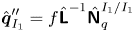 ${\hat{\boldsymbol{q}}}_{I_1}^{\prime \prime }= f {\hat {\boldsymbol{\mathsf{L}}}}^{-1}{\skew2\hat{\boldsymbol{\mathsf{N}}}}^{I_1/I_1}_q$. Here
 ${\skew2\hat{\boldsymbol{\mathsf{N}}}}^{I_1/I_1}_q$ stands for the nonlinear contribution due to the interaction of mode
 $I_1$ with itself (
 $I_1$ standing for either mode S or F), and it is computed as
 ${\skew2\hat{\boldsymbol{\mathsf{N}}}}^{I_1/I_1}_q ={\skew2\hat{\boldsymbol{\mathsf{N}}}_q}(\bar \rho, \bar u ,\ldots ; {\hat \rho }^{\prime }_{I_1} {\hat u}^{\prime }_{I_1},{\hat \rho }^{\prime }_{I_1} {\hat v}^{\prime }_{I_1},\ldots )$.
The streamwise distributions of the amplitude of the nonlinear interaction contribution (integrated in the wall-normal direction in the subsonic layer) are reported in figure 7 for the streamwise and wall-normal velocity modes and for the temperature mode, considering self-interactions (of the type S/S and F/F) and cross-interactions. For the latter, we consider both the initially unstable/initially stable mode interactions (S/F for  $M=4.5$ and F/S for
 $M=5.5$) and the initially stable/initially unstable mode interactions (F/S for
 $M=4.5$ and S/F for
 $M=5.5$). In the figure, the nonlinear terms
 ${\hat N}_u$,
 ${\hat N}_v$ and
 ${\hat N}_T$ are normalized by the corresponding total time rate of change, namely
 $\int _{0}^{y_s} |{\hat N}_u |/| {\hat {\rm D} \hat u}/{{\rm D} t}| \,{{\rm d}y}$,
 $\int _{0}^{y_s} |{\hat N}_v |/|{\hat {\rm D} \hat v}/{{\rm D} t}| \,{{\rm d}y}$ and
 $\int _{0}^{y_s} |{\hat N}_T |/|{\hat {\rm D} \hat T}/{{\rm D} t}|\,{{\rm d}y}$.
Streamwise distribution of the amplitude of the nonlinear interaction term integrated in the wall-normal direction at synchronization location: initially unstable ( $M=4.5$, S;
 $M=5.5$; F)/initially stable mode (
 $M=4.5$, F;
 $M=5.5$; S) interaction (
 $M=4.5$, S/F;
 $M=5.5$; F/S) and initially stable (
 $M=4.5$, F;
 $M=5.5$; S)/initially unstable mode (
 $M=4.5$, S;
 $M=5.5$; F) interaction (
 $M=4.5$, F/S;
 $M=5.5$; S/F). Note that in the legend,
 ${\hat N}_{u}^{*}$,
 ${\hat N}_{v}^{*}$ and
 ${\hat N}_{T}^{*}$ stand for normalized quantities, namely
 $\int _{0}^{y_s} |{\hat N}_u |/| {\hat {\rm D} \hat u}/{{\rm D} t}| \,{{\rm d}y}$,
 $\int _{0}^{y_s} |{\hat N}_v |/|{\hat {\rm D} \hat v}/{{\rm D} t}| \,{{\rm d}y}$ and
 $\int _{0}^{y_s} |{\hat N}_T |/| {\hat {\rm D} \hat T}/{{\rm D} t}| \,{{\rm d}y}$. (a)
 $M=4.5$; (b)
 $M=5.5$.

The contributions to second-order modes resulting from the interactions of first-order modes are negligible for the  ${\hat u}$ and
 ${\hat v}$ modes, and rather small for
 ${\hat T}$ modes. No significant changes occur as the modes evolve in the streamwise direction when crossing the synchronization location, and this for both self- and cross-interactions.
5. Governing equations for energy transfer analysis
Hypersonic boundary layer stability is characterized by the occurrence of fast and slow modes, whose spatial evolution depends on the thermal surface state and on the geometrical surface properties (Fedorov Reference Fedorov2011; Fedorov & Tumin Reference Fedorov and Tumin2011). Temperature disturbances also play an important role in hypersonic boundary layer stability because of the energy exchanges between internal and kinetic disturbance energies (Zhu et al. Reference Zhu, Lee, Chen, Wu, Chen and Gad-el Hak2018b). To elucidate the underlying physical mechanisms, and in particular to understand whether the mode spatial evolution is inviscid or viscous driven, we have analysed the transfer mechanisms between disturbance kinetic energy and temperature disturbance energy. In this process, the entropy ( $s$), the disturbance kinetic energy (in the following, we use, respectively, the symbols
 $k^\prime$ and
 $k^{\prime \prime }$ to refer to the perturbation kinetic energy of the first- and second-order modes) and the temperature perturbation energy (similarly, we introduce
 $k_T^\prime$ and
 $k_T^{\prime \prime }$) play an important role. To unravel the role in the amplification/suppression of the effects of the wall thermal state, their evolutions are analysed in detail.
5.1. Entropy, kinetic energy and ‘temperature energy’ budgets
In the following, we briefly derive the instantaneous governing equations for the entropy, the kinetic energy ( $k$) and the ‘temperature energy’ variable (
 $k_T$). For the sake of the analysis, we introduce the dimensionless entropy variable
 $\tilde {s}=s/c_p$ defined as
 \begin{equation} \tilde{s}= \ln\left(\frac{T}{T_{\infty}}\right)-\frac{R}{c_p} \ln\left(\frac{p}{p_{\infty}}\right)+ \tilde{s}_{\infty}. \end{equation}
The transport equation for  $\tilde {s}$ is obtained by using the Gibbs relation that gives
 \begin{equation} \frac{\partial s}{\partial t}+ u_j \frac{\partial s}{\partial x_j}= \underbrace{-\frac{1}{\rho c_p} \frac{\partial J_{s,j}}{\partial x_j }}_{\text{(i)}} +\underbrace{\frac{1}{c_p T} \phi}_{\text{(ii)}}+\underbrace{\frac{1}{c_p} \phi_T}_{\text{(iii)}}, \end{equation}
with
 \begin{equation} J_{s,j}={-}\frac{1}{T}\frac{\mu}{Pr}\frac{\partial T}{\partial x_j } \quad\text{and}\quad \rho\phi_T =J_{s,j}\left(-\frac{1}{T}\frac{\partial T}{\partial x_j}\right), \end{equation}
where  $\widetilde {()}$ has been dropped. Term (i) is the entropy diffusion flux associated with heat conduction, whereas terms (ii) and (iii) represent, respectively, the entropy production associated with viscous dissipation and energy exchanges by heat conduction.
The budget of the kinetic energy  $(k=(u^2+v^2+w^2)/2)$ is derived by taking the scalar product of the momentum budget and the velocity vector, yielding
 \begin{equation} \frac{\partial k}{\partial t}+ u_j \frac{\partial k}{\partial x_j}= \underbrace{-\frac{\partial u_j p}{\partial x_j}}_{\text{(i)}}+ \underbrace{\frac{p}{\rho} \frac{\partial u_j}{\partial x_j}}_{\text{(ii)}} +\underbrace{\frac{1}{\rho}\frac{\partial u_i \sigma_{ij}}{\partial x_j}}_{\text{(iii)}} \underbrace{-\phi}_{\text{(iv)}}. \end{equation}
The various terms on the right-hand side of (5.3) represent the pressure work (i), the pressure–dilatation (ii), the diffusion of kinetic energy (iii) and its dissipation due to viscous effects (iv). Introducing the energy variable (in a mathematical sense)  $k_T=T^2/2$, its governing equation is derived by multiplying the internal energy budget (expressed in terms of
 $T$, (2.1c)) by the temperature, thus obtaining
 \begin{equation} \frac{\partial k_T}{\partial t}+ u_j \frac{\partial k_T}{\partial x_j}= \underbrace{-\frac{1}{\rho c_v}Tp\frac{\partial u_j}{\partial x_j}}_{\text{(i)}} +\underbrace{\frac{\gamma}{\rho Pr} \frac{\partial}{\partial x_j} \left(\mu \frac{\partial k_T}{\partial x_j}\right)}_{\text{(ii)}} +\underbrace{\frac{1}{c_v}T \phi}_{\text{(iii)}} \underbrace{-\phi_{k_T}}_{\text{(iv)}}, \end{equation}
with
 \begin{equation} \phi_{k_T}=\frac{\gamma}{Pr}\nu\left(\frac{\partial T}{\partial x_j}\right)^2. \end{equation}
The terms on the right-hand side of (5.4a) represent the contribution due to pressure–dilatation (i), the exchange due to heat conduction (ii), the production associated with viscous dissipation of kinetic energy (iii) and the effects of thermal power dissipation associated with heat conduction (iv).
Inspection of (5.2a), (5.3) and (5.4a) shows the following:
(i) Pressure–dilatation (terms (ii) of (5.3) and (i) of (5.4a)) is a reversible inviscid energy transfer mechanism and it has an increasingly important role as the Mach number increases.
(ii) The action of viscous forces is an irreversible energy transfer mechanism (i.e. associated with entropy production through term (iii) of (5.2a)) that has a tendency to suppress mechanical energy (through term (iv) of (5.3)) and to amplify the energy variable
$k_T$ (term (iii) of (5.4a)), and its effect increases with the Mach number (having an impact on the scales, and hence on the receptivity of the boundary layer).(iii) The energy exchange due to heat conduction is an irreversible process (term (ii) of (5.2a)) whose action is toward suppressing
$k_T$ (term (iv) of (5.4a)).


5.2. Governing equations for the entropy disturbances, the disturbance kinetic energy and temperature disturbance energy
To shed some light on the physical mechanisms driving early-stage disturbance evolution and the associated energy transfer mechanisms, we have analysed the budgets of the entropy disturbances and of the disturbance kinetic and temperature disturbance energies up to second order.
5.2.1. Entropy disturbances
To derive the equations for the entropy disturbances, we first expand the thermodynamic (5.1) and the constitutive (5.2) relations up to second order, thus obtaining
 $$\begin{gather} \bar s = \ln\left(\frac{\bar T}{T_{\infty}}\right)-\frac{R}{c_p} \ln\left(\frac{\bar p}{p_{\infty}}\right) + {\bar s_{\infty}},\quad {\bar J}_{s,j} ={-}\frac {1}{\bar T}\frac{\bar\mu}{Pr}\frac{\partial \bar T}{\partial x_j}, \end{gather}$$
 $$\begin{gather}s^{\prime}= \frac{T^{\prime}}{\bar T}-\frac{R}{c_p}\frac{p^{\prime}}{\bar p},\quad J_{s^{\prime},j} ={-}\frac{\bar\mu}{Pr} \frac{\partial}{\partial x_j}\left(\frac {T^{\prime}}{\bar T}\right)=J^{\prime}_{s,j}, \end{gather}$$
 $$\begin{gather}s^{\prime\prime}= \frac{T^{\prime\prime}}{\bar T}-\frac{R}{c_p}\frac{p^{\prime\prime}}{\bar p}-\frac{1}{2}\left[\left(\frac {T^{\prime}}{\bar T}\right)^2-\frac{R}{c_p} \left(\frac {p^{\prime}}{\bar p}\right)^2\right],\quad J_{s^{\prime\prime},j} = J^{\prime\prime}_{s,j} +\frac{\bar\mu}{2Pr}\frac{\partial}{\partial x_j}\left(\frac {T^{\prime}}{\bar T}\right)^2. \end{gather}$$
The governing equations for the entropy disturbances are then obtained introducing the second-order decomposition in (5.2a) and using (5.5a)–(5.5c), thus giving
 \begin{align} \frac{\partial s^{(n)}}{\partial t}+\bar u_j \frac{\partial s^{(n)}}{\partial x_j} &= \frac{\bar \nu}{Pr} \frac{\partial^2 }{\partial x_j^2}\left(\frac {T^{(n)}}{\bar T}\right) +\frac{1}{Pr \bar \rho}\frac{\partial}{\partial x_j }\left(\frac {T^{(n)}}{\bar T}\right) \frac{\partial {\bar \mu}}{\partial x_j }\nonumber\\ &\quad +\frac{1}{c_p \bar T} \phi_L^{(n)}+\frac{1}{Pr \bar T} \phi_{T,L}^{(n)}-\frac{1}{\bar \rho}({\rho}^{(n)}{\bar u_j}+{\bar \rho}u^{(n)}_j) \frac{\partial {\bar s}}{\partial x_j} \nonumber\\ &\quad +(n-1)f (N_{B,s}^{(n)}+N_{S,s}^{(n)}), \end{align}
where  $n=1,2$, and
 \begin{equation} \phi_{T,L}^{(n)}=2{\bar \nu}\left(\frac{1}{\bar T}\frac{\partial {\bar T}}{\partial x_j}\right) \frac{\partial}{{\partial x}_j}\left(\frac {T^{(n)}}{\bar T}\right) \end{equation}
is the linearized thermal power dissipation (associated with heat conduction). The terms  $N_{B,s}^{(n)}$ and
 $N_{S,s}^{(n)}$ account for the nonlinear contributions associated with lower-order-mode interactions. For
 $n=1$,
 $N_{B,s}^{(1)}=0$ and
 $N_{S,s}^{(1)}=0$; for
 $n=2$,
 $$\begin{gather} N_{B,s}^{(2)}={-}\frac{\rho^{\prime}}{\bar \rho}\frac{\partial s^{\prime}}{\partial t }-\frac{1}{\bar \rho}({\rho}^{\prime}{\bar u_j}+{\bar \rho}{u^{\prime}_j})\frac{\partial s^{\prime}}{\partial x_j } -\frac{\rho^{\prime}}{\bar \rho}u^{\prime}_j \frac{\partial {\bar s}}{\partial x_j }, \end{gather}$$
 $$\begin{gather}N_{S,s}^{(2)}= \frac{1}{c_p \bar T}\left[\phi^{\prime}-\frac{T^{\prime}}{\bar T} \phi^{\prime}_L+\frac {1}{2} \left(\frac{T^{\prime}}{\bar T}\right)^2 {\bar \phi}\right] -\frac{1}{2Pr}\frac{\partial}{\partial x_j} \left[ \bar\mu \frac{\partial}{\partial x_j}\left(\frac {T^{\prime}}{\bar T}\right)^2 \right], \end{gather}$$
with  ${\bar \phi }={\bar \nu } [ 2{\bar S}_{ij}{\bar S}_{ij}-\frac {2}{3}{{\bar S}}_{\ell \ell }{{\bar S}}_{kk} ]$ the base flow dissipation.
Dropping superscript  $(n)$ (unless confusion arises) and introducing the normal-mode expansion in (5.6), gives
 \begin{equation} \frac{\hat {\rm D}{\hat s}}{{\rm D} t }+{\bar v} \frac{{\rm d} \hat s}{{\rm d}y} = D_s +{\hat \phi}_{s,u}+{\hat \phi}_{s,T}+{s\textit{-}mgP}+(n-1)f {\hat N}_{s}, \end{equation}
where  $D_s$ and
 ${s\textit {-}mgP}$ represent, respectively, the normal-mode forms of the diffusion and the base flow entropy gradient generation contributions, and
 ${\hat \phi }_{s,u}$ and
 ${\hat \phi }_{s,T}$ are the normal-mode form of the entropy generation rates associated with viscous and heat conduction effects, with
 \begin{gather}\begin{aligned}[b] D_s &= \frac{\bar \nu}{Pr}
\left[\left(\alpha^2-{\rm i}\frac{{\rm d} \alpha}{{\rm d}\kern 0.06em x}\right) \frac{\hat T}{\bar T}+2 {\rm i} \alpha {\hat T}
\frac{\partial}{\partial x }\left(\frac{1}{\bar T}\right)
+{\hat T}\frac{\partial^2}{\partial x^2
}\left(\frac{1}{\bar T}\right) \right.\nonumber\\ &\quad
\left.+\frac{1}{\bar T}\frac{{\rm d}^2 {\hat T}}{{{\rm
d}y}^2 }+2 \frac{{\rm d} {\hat T}}{{{\rm d}y}
}\frac{\partial}{\partial y }\left(\frac{1}{\bar T}\right)
+{\hat T}\frac{\partial^2}{\partial y^2
}\left(\frac{1}{\bar T}\right)\right] \nonumber\\ &\quad
+\frac{1}{Pr} \frac{1}{\bar \rho} \left[ {\rm i} \alpha
\frac{{\hat T}}{\bar T}+{\hat T} \frac{\partial}{\partial x
} \left (\frac{1}{\bar T} \right)\right]\frac{1}{\bar T}
\frac{\partial {\bar \mu}}{\partial x} +\frac{1}{Pr}
\frac{1}{\bar \rho}\left[\frac{1}{\bar T} \frac{{\rm d}
{\hat T}}{{{\rm d}y}}+{\hat T} \frac{\partial}{\partial y }
\left( \frac{1}{\bar T}\right)\right] \frac{\partial {\bar
\mu}}{\partial y}, \end{aligned}
\end{gather}
 $$\begin{gather} {s\textit{-}mgP}={-}\left[{\hat u}+{\bar u}\left(\frac{\hat p}{\bar p}-\frac{\hat T}{\bar T}\right)\right]\frac{\partial {\bar s}}{\partial x } -\left[{\hat v}+{\bar v}\left(\frac{\hat p}{\bar p}-\frac{\hat T}{\bar T}\right)\right]\frac{\partial {\bar s}}{\partial y }, \end{gather}$$
 $$\begin{gather}{\hat \phi}_{s,u}=\frac{1}{c_p \bar T}{{\hat \phi}_L}, \end{gather}$$
 $$\begin{gather}{\hat \phi}_{s,T}=\frac{1}{\bar T} {{\hat \phi}_{T,L}}, \end{gather}$$
where
 \begin{equation} {\hat \phi}_{T,L}=2\frac{\bar \nu}{Pr} \left\{\left[\frac{1}{\bar T} \frac{\partial \bar T}{\partial x } \frac{1}{\bar T} i \alpha {\hat T} +{\hat T}\frac{\partial}{\partial x } \left(\frac{1}{\bar T}\right) \right]+\left[\frac{1}{\bar T} \frac{\partial \bar T}{\partial y }\frac{1}{\bar T} \frac{{\rm d} \hat T}{{{\rm d}y} } +{\hat T} \frac{\partial}{\partial y }\left(\frac{1}{\bar T}\right) \right]\right\} \end{equation}
and  ${\hat \phi }_L$ is defined in (4.16d). Terms
 ${{\hat N}_{B,s}}$ and
 ${{\hat N}_{S,s}}$ are the normal-mode forms of the mode interaction terms:
 $$\begin{gather} {\hat N}_{B,s}= {\rm i} \omega \frac{{\hat \rho}^{\prime}}{\bar \rho}{\hat s^{\prime}} -{\rm i} \alpha \frac{1}{\bar \rho}({\hat \rho}^{\prime}{\bar u}+{\bar \rho}{{\hat u}^{\prime}}){\hat s^{\prime}} - \frac{1}{\bar \rho}({\hat \rho}^{\prime}{\bar v}+{\bar \rho}{{\hat v}^{\prime}})\frac{{\rm d} \hat s^{\prime}}{{{\rm d}y} } -\frac{{\hat \rho}^{\prime}}{\bar \rho} {\hat u}^{\prime} \frac{\partial {\bar s}}{\partial x }-\frac{{\hat \rho}^{\prime}}{\bar \rho} {\hat v}^{\prime}\frac{\partial {\bar s}}{\partial y }, \end{gather}$$
 $$\begin{gather}{\hat N}_{S,s}= \frac{1}{c_p \bar T} \left[{\hat \phi}^{\prime}-\frac{ {\hat T}^{\prime}}{\bar T} {\hat \phi}^{\prime}_L+\frac {1}{2}\left(\frac{ {\hat T}^{\prime}}{\bar T}\right)^2 {\bar \phi}\right] -\frac{1}{2Pr}\frac{\partial}{\partial x_j} \left[ \bar\mu \frac{\partial}{\partial x_j}\left(\frac {{\hat T}^{\prime}}{\bar T}\right)^2 \right]. \end{gather}$$
Note that unless otherwise specified, here and in the following  $\widehat {(\cdot )}$ stands for either the first- or the second-order mode, respectively.
5.2.2. Disturbance kinetic energy
Let  $\hat k^{\prime }$ and
 $\hat k^{\prime \prime }$ be the disturbance kinetic energy, respectively, of the first- and second-order velocity disturbance mode. Defining
 $\hat k^{\prime }={\mathcal {R}}({\hat u^{\prime }_i}){\mathcal {R}}({\hat u^{\prime }_i})/2$ and
 $\hat k^{\prime \prime }={\mathcal {R}}({\hat u^{\prime \prime }_i}){\mathcal {R}}({\hat u^{\prime \prime }_i})/2$,
 ${\mathcal {R}}(\cdot )$ denoting the real part, the governing equations for the disturbance kinetic energies are readily obtained by multiplying the real part of the
 $n$th-order normal-mode form of (3.13b) by the real part of the
 $n$th-order velocity disturbance mode
 ${\mathcal {R}}({\hat u}^{(n)}_i)$. Dropping superscript
 $(n)$, one has
 \begin{equation} {\mathcal{R}}({\hat u}_i){\mathcal{R}} \left[\!\frac{\partial {\hat u}_i}{\partial t}+\bar u_j \frac{\partial {\hat u}_i}{\partial x_j} +\frac{1}{\bar \rho}\frac{\partial {\hat p}}{\partial x _i} -\frac{1}{\bar \rho}\frac{\partial {\hat \sigma}_{ij}}{\partial x_j} +\frac{1}{\bar \rho}({\hat \rho}{\bar u_j}+{\bar \rho}{\hat u}_j) \frac{\partial {\bar u_i}}{\partial x_j}\!\right] =(n-1){\mathcal{R}}({\hat u}_i) {\mathcal{R}} (f {{\hat{N}}_{u_i}}).\end{equation}
The governing equation for  $\hat k$ (
 $\hat k$ standing for either
 ${\hat k}^{\prime }$ or
 ${\hat k}^{\prime \prime }$) is then written as
 \begin{equation} \frac{\hat {\rm D} \hat k}{{\rm D} t}+{\bar v} \frac{{\rm d} \hat k}{{\rm d}y}={-}\frac{1}{\bar \rho}{\varPi}_{W}+ \frac{1}{\bar \rho}{\varPi}_{\theta}+D_{k}-{\phi}+P_{k}+(n-1){\hat{\mathcal{N}}}_k, \end{equation}
where  ${\varPi }_{W}$,
 ${\varPi }_{\theta }$,
 $D_{k}$,
 ${\phi }$ and
 $P_{k}$ are, respectively, the disturbance pressure work, the pressure–dilatation, the diffusion of disturbance kinetic energy and its dissipation due to viscous effects and the production resulting from base flow/mode interaction driven by mean velocity gradients:
 $$\begin{gather} {\varPi}_{W}=\frac{\partial}{\partial x _i} [{\mathcal{R}}({\hat p}){\mathcal{R}}({\hat u}_i)], \end{gather}$$
 $$\begin{gather}{\varPi}_{\theta}= {\mathcal{R}}({\hat p})\frac{\partial }{\partial x _i} [{\mathcal{R}}({\hat u}_i)], \end{gather}$$
 $$\begin{gather}D_{k}= \frac{1}{\bar \rho}\frac{\partial }{\partial x _i} [{\mathcal{R}}({\hat u}_i) {\mathcal{R}}({\hat \sigma}_{ij})], \end{gather}$$
 $$\begin{gather}{\phi}=\frac{1}{\bar \rho} {\mathcal{R}}({\hat S}_{ij}){\mathcal{R}}({\hat \sigma}_{ij}), \end{gather}$$
 $$\begin{gather}P_{k}={-}\frac{1}{\bar \rho}\{{\mathcal{R}}({\hat u}_i)[{\mathcal{R}}({\hat \rho}){\bar u_j}+{\bar \rho} {\mathcal{R}}({\hat u}_j)]\} \frac{\partial {\bar u_i}}{\partial x_j }. \end{gather}$$
The term  $\hat {\mathcal {N}}_k$ is the contribution to the higher-order disturbance kinetic energy resulting from first-order mode interactions, defined as
 \begin{equation} \hat{\mathcal{N}}_k={\mathcal{R}}({\hat u}_i){\mathcal{R}}(f {{\hat{N}}_{u_i}}), \end{equation}
with
 \begin{equation} {\hat N}_{u_i}= \frac{1}{\bar \rho} \left[{\rm i} \omega {\hat \rho}^{\prime}{\hat u_i^{\prime}} -{\rm i}\alpha ({\hat \rho}^{\prime}{\bar u}+{\bar \rho}{{\hat u}^{\prime}}){\hat u_i^{\prime}} -({\hat \rho}^{\prime}{\bar v}+{\bar \rho}{{\hat v}^{\prime}}) \frac{{\rm d} \hat u_i^{\prime}}{{{\rm d}y} }-{\hat \rho}^{\prime} {\hat u}^{\prime} \frac{\partial {\overline{u_i}}}{\partial x}-{\hat \rho}^{\prime} {\hat v}^{\prime} \frac{\partial {\overline{u_i}}}{\partial y}\right]. \end{equation}
5.2.3. Temperature disturbance energy
Let  ${\hat{k}_T^{\prime }}$ and
 ${\hat k_T^{\prime \prime }}$ be the temperature disturbance energy, respectively, of the first- and second-order temperature disturbance mode. Defining
 ${\hat k_T^{\prime }}={\mathcal {R}}({\hat T^{\prime }}){\mathcal {R}}({\hat T^{\prime }})/2$ and
 ${\hat k_T^{\prime \prime }}={\mathcal {R}}({\hat T^{\prime \prime }}){\mathcal {R}}({\hat T^{\prime \prime }})/2$, the governing equations for the temperature disturbance energies are readily obtained by multiplying the real part of the
 $n$th-order normal-mode form of (3.13c) by the real part of the
 $n$th-order temperature disturbance mode
 ${\mathcal {R}}({\hat T}^{(n)})$. Dropping superscript
 $(n)$, one has
 \begin{align} & {\mathcal{R}}({\hat T}){\mathcal{R}}\left\{\frac{\partial {\hat T}}{\partial t}+\bar u_j \frac{\partial {\hat T}}{\partial x_j}+\frac{1}{\bar \rho c_v} \left[{\hat p}\frac{\partial \bar u_i}{\partial x_i} +\bar p\frac{\partial {\hat u}_i}{\partial x_i}\right] -\frac{\gamma}{Pr \bar \rho } \frac{\partial}{\partial x_j}\left[{\bar \mu} \frac{\partial {\hat T}}{\partial x_j}\right]\right\} \nonumber\\ &\quad +{\mathcal{R}}({\hat T}){\mathcal{R}}\left\{-\frac{1}{c_v}{{\hat \phi}_L} +\frac{1}{\bar \rho}\left[{{\hat \rho}}{\bar u_j}+{\bar \rho}{\hat u}_j\right] \frac{\partial {\bar T}}{\partial x_j}\right\} =(n-1) {\mathcal{R}}({\hat T}) {\mathcal{R}}(f {\hat{N}}_T). \end{align}
The governing equation for  $\hat k_T$ (
 $\hat k_T$ standing for either
 ${\hat k_T^{\prime }}$ or
 ${\hat k_T^{\prime \prime }}$) is then written as
 \begin{equation} \frac{\hat {\rm D} \hat k_T}{{\rm D} t}+{\bar v} \frac{{\rm d} \hat k_T}{{\rm d}y}={-} \frac{1}{\bar \rho}{\varPi}_{{\theta},T}+ D_{k_T}+{\phi}_u-{\phi}_{k_T}+P_{k_T}+(n-1) \hat{\mathcal{N}}_{k_T}, \end{equation}
where  ${\varPi }_{{\theta },T}$,
 $D_{k_T}$,
 ${\phi }_u$,
 ${\phi }_{k_T}$ and
 $P_{k_T}$ are, respectively, the (normal-mode form of the) temperature disturbance energy transfer associated with pressure–dilatation, the exchange of temperature disturbance energy due to heat conduction, the production due to viscous effects, the thermal power temperature disturbance energy loss and the production resulting from base flow/mode interaction driven by mean temperature gradients:
 $$\begin{gather} {\varPi}_{{\theta},T}=\frac{1}{c_v} {\mathcal{R}}({\hat T}){\mathcal{R}}\left({\hat p}\frac{\partial \bar u_i}{\partial x_i }+\bar p\frac{\partial {\hat u}_i}{\partial x_i }\right), \end{gather}$$
 $$\begin{gather}D_{k_T}=\frac{\gamma}{Pr} \frac{1}{\bar \rho}\frac{\partial}{\partial x_j}\left[{\mathcal{R}}({\hat T}){\bar \mu} {\mathcal{R}}\left(\frac{\partial {\hat T}}{\partial x_j}\right)\right], \end{gather}$$
 $$\begin{gather}{\phi}_u=\frac{1}{c_v}{\mathcal{R}}({\hat T}) {\mathcal{R}}({{\hat \phi}_L}), \end{gather}$$
 $$\begin{gather}{\phi}_{k_T}=\frac{\gamma}{Pr}{\bar \nu}\frac{\partial {\mathcal{R}}({\hat T})}{\partial x_j} \frac{\partial {\mathcal{R}}({\hat T})}{\partial x_j}, \end{gather}$$
 $$\begin{gather}P_{k_T}={-}\frac{1}{c_v \bar \rho} {\mathcal{R}}({\hat T})[{\mathcal{R}}({\hat \rho}{\bar u_j}+{\bar \rho} {\hat u}_j)] \frac{\partial {\bar T_i}}{\partial x_j }. \end{gather}$$
The term  $\hat {\mathcal {N}}_{k_T}$ is the contribution to the higher-order temperature disturbance energy resulting from first-order mode interactions, defined as
 \begin{equation} \hat{\mathcal{N}}_{k_T}={\mathcal{R}}({\hat T}){\mathcal{R}}(f {{\hat{N}}_T}), \end{equation}
with
 \begin{align} {\hat N}_T &= \frac{1}{\bar \rho c_v} \left[{\rm i} \omega {\hat \rho}^{\prime}{\hat T^{\prime}} - {\rm i}\alpha ({\hat \rho}^{\prime}{\bar u}+{\bar \rho}{{\hat u}^{\prime}}){\hat T^{\prime}} - ({\hat \rho}^{\prime}{\bar v}+{\bar \rho}{{\hat v}^{\prime}}) \frac{{\rm d} \hat T^{\prime}}{{{\rm d}y}}-{\hat \rho}^{\prime} {\hat u}^{\prime} \frac{\partial {\bar T}}{\partial x }-{\hat \rho}^{\prime} {\hat v}^{\prime} \frac{\partial {\bar T}}{\partial y }\right]\nonumber\\ &\quad - \frac{1}{\bar \rho c_v}{\hat p}^{\prime} \left({\rm i}\alpha{\hat u}^{\prime}+ \frac{{\rm d} \hat v^{\prime}}{{{\rm d}y} }\right)+ \frac{1}{c_v}{\hat \phi}^{\prime}. \end{align}
Unless confusion arises, in the following  ${\mathcal {R}}(\cdot )$ is omitted for ease of reading. Equations (5.14) and (5.19) show that at higher order, the disturbance kinetic and temperature disturbance energies are driven not only by inviscid mechanisms associated with dilatational effects, base flow/disturbance interaction and the combined actions of viscous and heat conduction effects (as for the lower-order case), but also by velocity, pressure and temperature mode interactions. The equations show that disturbance kinetic energy is drained by the action of viscous dissipation
 ${\phi }$, whereas temperature disturbance energy is produced by the action of linearized viscous dissipation (term
 ${\hat T} {{\hat \phi }_L}/{c_v}$ of (5.20c)) and is dissipated by heat conduction effects (term
 ${\phi }_{k_T}$).
5.2.4. Near-wall disturbance entropy and perturbation energy behaviour
In the near-wall vicinity, the entropy, the perturbation kinetic energy and the temperature perturbation energy equations (5.6), (5.14) and (5.19) reduce to
 $$\begin{gather} -{\rm i}\omega{\hat s} =\frac{1}{Pr}\frac{1}{\bar \rho} \frac{\partial}{\partial y}\left[{\bar \mu}\frac{{\rm d}}{{\rm d}y}\left(\frac{\hat T}{\bar T}\right)\right]+\frac{1}{c_p {\bar T}}{\hat\phi}_{L} +\frac{1}{{\bar T}}{\hat\phi}_{T,L}, \end{gather}$$
 $$\begin{gather}\frac{\partial}{\partial y}\left({\bar \mu}\frac{{\rm d} \hat k}{{{\rm d}y} }\right)= {\bar \rho}{\phi}, \end{gather}$$
 $$\begin{gather}\frac{\gamma}{Pr} \frac{\partial}{\partial y}\left({\bar \mu}\frac{{\rm d} \hat k_T}{{{\rm d}y} }\right)= {\bar \rho}{\phi}_{k_T} , \end{gather}$$
where
 \begin{equation} \left.\begin{gathered}
{\hat \phi}_{L} = 2{\bar \nu}\left[\frac{4}{3}
\frac{\partial \bar v}{\partial y } {\mathcal{R}}
\left(\frac{{\rm d} {\hat v}}{\partial y
}\right)+\frac{\partial \bar u}{\partial y } {\mathcal{R}}
\left(\frac{{\rm d} {\hat u}}{\partial y }\right)\right],\\
{\hat \phi}_{T,L}=2\frac{\bar \nu}{Pr}\left[\frac{1}{\bar
T} \frac{\partial \bar T}{\partial y } \frac{1}{\bar T}
{\mathcal{R}}\left(\frac{{\rm d} {\hat T}}{\partial y
}\right)\right],\\ {\phi}={\bar \nu}
\left[{\mathcal{R}}\left(\frac{{\rm d} {\hat u}}{\partial y
}\right){\mathcal{R}} \left(\frac{{\rm d} {\hat
u}}{\partial y }\right)+\frac{4}{3}{\mathcal{R}}
\left(\frac{{\rm d} {\hat v}}{\partial y
}\right){\mathcal{R}}\left(\frac{{\rm d} {\hat v}}{\partial
y }\right)\right],\\ {\phi}_{k_T}=\frac{\gamma}{Pr} {\bar
\nu}{\mathcal{R}}\left(\frac{{\rm d} {\hat T}}{\partial y
}\right){\mathcal{R}} \left(\frac{{\rm d} {\hat
T}}{\partial y }\right).\end{gathered}\right\}
\end{equation}
Equations (5.23a)–(5.23c) show that at the wall
(i) there is no direct effect of mode interactions on both
$k$ and $k_T$;(ii) dissipation and diffusive transport of perturbation kinetic energy are in equilibrium; and
(iii) thermal power dissipation and transport associated with heat conduction of temperature perturbation energy are in equilibrium.


6. Energy analysis
6.1. Perturbation energy analysis
The discussion being centred on the understanding of the underlying energy transfer mechanisms, we scrutinize the contributions associated with the pressure–dilatation and the dissipation due to viscous and heat conduction effects on the perturbation kinetic energy and the temperature perturbation energy. In addition, to ascertain the role of the reversible versus the irreversible mechanisms we have also analysed in detail these effects on the entropy perturbation. For clarity, the terms that have been scrutinized are
 $$\begin{gather} \text{in the budget of}\ s:\quad \phi_{s,u}=\frac{1}{c_p \bar T} {\hat T} \phi_L,\quad \phi_{s,T}=\frac{1}{Pr \bar T} {\hat \phi_{T,L}}; \end{gather}$$
 $$\begin{gather}\text{in the budget of}\ \hat k:\quad \hat p \hat \theta,\quad -\phi_{S^2},\quad -\phi_{\theta^2}; \end{gather}$$
 $$\begin{gather}\text{in the budget of}\ \hat k_T:\quad -\frac{1}{c_v} {\hat T} (p \theta)_L,\quad \phi_u=\frac{1}{c_v} {\hat T} \phi_L,\quad -\phi_{k_T}, \end{gather}$$
 $$\begin{gather}\text{with}\quad {\bar \rho}\phi_{S^2}=2 {\bar \mu}{\mathcal{R}}({\hat S}_{ij}){\mathcal{R}}({\hat S}_{ij}),\quad {\bar \rho}\phi_{\theta^2} ={-}\frac{2}{3} {\bar \mu} {\mathcal{R}}({\hat \theta}){\mathcal{R}}({\hat \theta}). \end{gather}$$
Observe that the linearized thermal power dissipation  $\hat \phi _{T,L}$ (equation (5.11)) can in principle attain either non-negative or non-positive values, and, consequently, entropy perturbation can either increase or decrease due to (linearized) heat conduction. Similarly, entropy perturbation can either increase or decrease by the action of the linearized viscous dissipation, since
 $\hat \phi _L$ (equation (4.16d)) can in principle be either non-negative or non-positive. As also proposed in Zhu et al. (Reference Zhu, Zhu, Gu, Chen, Lee and Oran2020, Reference Zhu, Gu, Zhu, Chen, Lee and Oran2021), the dissipation of mechanical energy is expressed as the sum of two terms (
 $\phi =\phi _{S^2}+\phi _{\theta ^2}$), where
 $\phi _{S^2}$ accounts for the deformation work associated with the deformation tensor and
 $\phi _{\theta ^2}$ represents the contribution due to dilatational effects (equation (6.1d)). Observe that
 $\phi _{S^2}\geq 0$ (i.e.
 $k$ is dissipated due to the action of deformation work), whereas
 $\phi _{\theta ^2}\leq 0$ (i.e.
 $k$ is produced due to dilatational viscous dissipation effects).
The budgets of the slow and fast entropy perturbation modes are reported in figure 8. The figure shows that the primary physical mechanisms driving the entropy perturbation evolution are its diffusion (associated with heat conduction) and the base flow entropy gradient generation (s-mgP). The (linearized) viscous ( $({1}/{c_p \bar T}) {{{\hat \phi }_L}}$) and thermal power (
 $({1}/{\bar T}) {{\hat \phi }_{T,L}}$) dissipation contributions (in the discussion that follows their sum is also referred to as the entropy generation rate) are negligible except in very close proximity to the wall (but still small), where diffusion dominates. Across the critical layer, entropy perturbation is primarily controlled by mean base flow entropy gradient production, by transverse convection and diffusion and, to a lesser extent, by viscous dissipation (the latter contribution being somewhat more significant for the fast mode). Across the critical layer, diffusion plays a significant role in the slow (fast) mode for adiabatic (cold) wall.
Budgets of the entropy perturbation of modes S and F for (a) adiabatic wall ( $M=4.5$) and (b) cold wall (
 $M=5.5$).

The streamwise distributions of the generation rates integrated separately over the subsonic sublayer (in the range  $[0, y_s]$; this region is hereafter simply referred to as the subsonic region,
 $Sub$) and over the supersonic portion of the boundary layer above the sonic line (in the range
 $[y_s,\delta ]$,
 $\delta$ being the local boundary layer height; this region is hereafter simply referred to as the supersonic region,
 $Sup$) are reported in figure 9. The contribution of term
 $s$-
 $mgP$ (results not reported in the figure for clarity) is dominant, further confirming that dissipative effects are rather negligible. In the supersonic region (for both modes S and F), the generation rates are not in phase, whereas they are in phase in the subsonic portion of the boundary layer. In the subsonic region, for adiabatic wall, the contribution resulting from the effects due to viscous dissipation is more significant than that due to thermal power dissipation. The opposite holds true for cold wall.
Streamwise distributions of the entropy generation rate of modes S and F integrated in the wall-normal direction across the supersonic ( $Sup$) and subsonic (
 $Sub$) regions. The rates are normalized by
 $\max _x[\int _{}^{y} |{\partial s/\partial t}+\bar u {\partial s/\partial x}| \,{\textrm {d}y}]$. (a)
 $M=4.5$; (b)
 $M=5.5$.

In conclusion, entropy perturbations are driven primarily by an inviscid mechanism associated with base flow entropy gradient production (as already pointed out in the discussion of the entropy perturbation budgets at synchronization location). This indicates that to a good approximation, in the subsonic layer, where acoustic waves are trapped (Mack Reference Mack1984; Fedorov Reference Fedorov2011; Zhong & Wang Reference Zhong and Wang2012), the exchange of energy is a reversible process associated with pressure–dilatation.
The wall-normal budgets of the perturbation kinetic energy and of the temperature perturbation energy in the subsonic portion of the boundary layer at synchronization location are reported, respectively, in figures 10 and 11. Figure 10 shows that the perturbation kinetic energy is driven by the pressure work, pressure–dilation and base flow/perturbation interaction mechanisms. The slow mode undergoes positive pressure work near the wall, which changes sign moving away from the wall becoming negative at about  $1/3$ of the subsonic thickness. The pressure–dilatation term is predominantly negative draining perturbation kinetic energy. For mode F, the pressure work is negative near the wall and the pressure–dilatation is positive contributing to an increase of its perturbation kinetic energy. As in fully turbulent boundary layers, and in agreement with (5.23b), dissipation and diffusion of perturbation kinetic energy by viscous effects are in equilibrium at the wall. The budget of the temperature perturbation energy (figure 11) shows that thermal power dissipation and the exchanges associated with heat conduction are significant in the proximity of the wall, the two being in equilibrium at the wall (as predicted from (5.23c)).
Perturbation kinetic energy budget of modes S and F at synchronization location. (a)  $M=4.5$; (b)
 $M=5.5$.

Temperature perturbation energy budget of modes S and F at synchronization location. (a)  $M=4.5$; (b)
 $M=5.5$.

To better understand the underlying inviscid energy transfer mechanisms, we have scrutinized in more detail the dilatation and dissipation rates associated with viscous and heat conduction effects. Figure 12 reports the streamwise distributions of  $\hat p \hat \theta$ and
 $-\hat T(p \theta )_L/c_v$ for the adiabatic and cold-wall cases (
 $M=4.5$ and
 $M=5.5$, respectively) at
 $y=1/8 y_{s}$ and
 $y_{crit}$. As also found by Zhu et al. (Reference Zhu, Zhu, Gu, Chen, Lee and Oran2020, Reference Zhu, Gu, Zhu, Chen, Lee and Oran2021), the pressure–dilatation exhibits a nearly sinusoidal variation in the streamwise direction alternating between positive and negative values, and changes sign also in the wall-normal direction. For
 $M=4.5$ (and
 $M=6$ and
 $M=6.5$ cases, not reported) the slow mode (which is the initially unstable mode for these cases) experiences energy exchanges that grow in amplitude in the streamwise direction, whereas the fast mode undergoes a decaying energy exchange mechanism. The opposite holds true for
 $M=5.5$, for which the fast mode is initially unstable. The same features are observed for
 $-\hat T (p \theta )_L/c_v$.
Streamwise distributions of  $\hat p \hat \theta$ and
 $-\hat T{(p \theta )_L}$ of modes S and F at various wall-normal locations. (a)
 $M=4.5$; (b)
 $M=5.5$.

The wall-normal distributions at synchronization location are reported in figure 13. To second order, the slow mode experiences a local decrease of perturbation kinetic energy in the subsonic near-wall region (i.e.  $\hat p \hat \theta <0$). On the contrary, the pressure–dilatation contribution to the perturbation kinetic energy of mode F is positive (
 $\hat p \hat \theta >0$). Accordingly, for the slow mode, there is a transfer from mechanical to thermal perturbation energy (
 $p \theta <0$ and
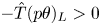 $-{\hat T}(p \theta )_L > 0$), whereas a reversed process is experienced by the fast mode (
 $\hat p \hat \theta >0$ and
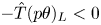 $-{\hat T}(p \theta )_L < 0$). In the subsonic region
 $\hat p \hat \theta$ and
 $-\hat T (p \theta )_L$ are in phase opposition (perturbation kinetic energy is produced through
 $\hat p \hat \theta$ at the expense of temperature perturbation energy through term
 $-\hat T (p \theta )_L$ and vice versa). As a consequence, we conclude that when
 $\hat p \hat \theta \gtrless 0$,
 $-\hat T {\bar p}{\theta } \lessgtr 0$, and if
 $\hat p$ and
 $\hat \theta$ are in phase (not in phase),
 $\hat T$ and
 $\hat \theta$ are also in phase (not in phase).
Wall-normal distributions of normalized energy exchange rates due to dilatational effects across synchronization location to second order. The horizontal lines indicate the height of the sonic line for slow and fast modes. (a)  $M=4.5$; (b)
 $M=5.5$.

It is interesting to observe that this bi-directionality is verified also to first order (figure 14). In principle, this result is not to be expected. Indeed, if it is true for the kinetic energy ( $u_i^2/2$) and the ‘energy variable’ (
 $T^2/2$) of the flow, the same conclusion cannot be reached a priori for the perturbation field at any order (i.e. when
 $\hat p \hat \theta \gtrless 0$,
 $-{\hat T}(p \theta )_L$ can take, in principle, any value). In figure 15 we report the wall-normal distributions of
 $(p \theta )_L$ and
 ${\bar p} \hat \theta$ up to second order. The figure shows that
 $(p \theta )_L \approx {\bar p} \hat \theta$ (i.e. the base flow dilatation is not significant in the establishment of the streamwise evolution of the linearized pressure–dilatation term).
Wall-normal distributions of first-order normalized energy exchange rates due to dilatational effects across synchronization location. (a)  $M=4.5$; (b)
 $M=5.5$.

Wall-normal distributions of  $(p \theta )_L$ and
 ${\bar p} {\hat \theta }$ across synchronization location. The horizontal lines indicate the height of the sonic line for slow and fast modes. (a)
 $M=4.5$; (b)
 $M=5.5$.

The observed change in sign of the pressure–dilatation indicates that a two-way reversible energy transfer process is established, alternating between cooling and heating in both the streamwise and wall-normal directions. The direction of this conversion process is determined by the sign of the phase difference between the pressure and the dilatation  $\cos (\varphi _p - \varphi _{\theta })$,
 $\varphi _p$ and
 $\varphi _{\theta }$ being the phase of
 $p$ and
 $\theta$, respectively (Zhu et al. Reference Zhu, Zhu, Gu, Chen, Lee and Oran2020, Reference Zhu, Gu, Zhu, Chen, Lee and Oran2021), where
 \begin{equation} \cos({\varphi}_p -
\varphi_{\theta}):=\frac{(p \theta)}{p_{rms}
\theta_{rms}}\quad \text{with}\ \left\{\begin{array}{@{}l@{}}
p=\bar p + \epsilon {\mathcal{R}} (\hat
p^{\prime})+\epsilon^2 {\mathcal{R}} (\hat
p^{\prime\prime}) \\ \theta={\bar \theta} + \epsilon
{\mathcal{R}} ({\hat \theta}^{\prime})+\epsilon^2
{\mathcal{R}} ({\hat \theta}^{\prime\prime}).
\end{array}\right. \end{equation}
Figure 16 shows the streamwise distribution of  $\cos ({\varphi }_p - \varphi _{\theta })$ in the subsonic (at
 $y=y_s/8$) and supersonic (at
 $y=y_{crit}$) regions across synchronization for
 $M=4.5$ and
 $M=5.5$. The wall-normal distributions at three different streamwise locations (before, at and past synchronization) are displayed in figure 17. The figures show that in the subsonic region the phase difference (
 $\varphi _p-\varphi _{\theta }$) varies periodically in the streamwise direction assuming positive and negative values, and it is approximately constant in the wall-normal direction. For
 $M=4.5$, the initially unstable mode (mode S) experiences mild heating/cooling/heating as it evolves in the near-wall layer and cooling moving away from the wall. Similarly, for
 $M=5.5$, the initially unstable mode (mode F) experiences cooling/heating/cooling in the near-wall region and undergoes cooling farther away from the wall. It is also interesting to observe that at first order (
 $\varphi _p-\varphi _{\theta }$) does not vary with
 $x$ (figure 17), in agreement with the findings of Zhu et al. (Reference Zhu, Zhu, Gu, Chen, Lee and Oran2020).
Streamwise distributions of  $\cos (\varphi _p - \varphi _{\theta })$ at
 $y=y_{crit}$ (
 $Sup$) and
 $y=y_s/8$ (
 $Sub$). Thin lines, first order; thick lines, up to second order. (a)
 $M=4.5$; (b)
 $M=5.5$.

Wall-normal distributions of  $\cos (\varphi _p - \varphi _{\theta })$ at synchronization location. Thin lines, first order; thick lines, up to second order. (a)
 $M=4.5$; (b)
 $M=5.5$.

The streamwise distributions of  $\phi _{S^2}$ and
 $\phi _{\theta ^2}$ (generically referred to as dissipation rates of the perturbation kinetic energy) and of
 $\hat T {\phi }_L/{c_v}$ and
 ${\phi }_{k_T}$ (generically referred to as the generation rates of the temperature perturbation energy) are reported in figure 18. The dissipation and generation rates are normalized, respectively, by the local
 $\max _x |\hat p \hat \theta |$ and
 $\max _x |\hat T(p \theta )_L/c_v|$. The figure shows that the dilatational part of the deformation work is smaller than that associated with the deformation tensor (that contributes to local heating, even though negligible). In addition, thermal power dissipation is larger than the linearized viscous dissipation of temperature perturbation energy. As previously observed when discussing the entropy budget, the irreversible exchanges are much smaller than the reversible ones (
 $\hat p \hat \theta$ and
 $-\hat T(p \theta )_L/c_v$, not reported in the figure for clarity). It is also interesting to observe that the irreversible energy exchange rates exhibit the same feature as the reversible ones. Namely, the initially unstable modes (the slow and fast modes, respectively, for
 $M=4.5$ and
 $M=5.5$) undergo an irreversible energy exchange process that grows in amplitude in the streamwise direction, whereas the initially stable modes undergo rapidly decaying energy exchanges.
Streamwise distributions of the dissipation ( $\phi _{\theta ^2}$ and
 $\phi _{S^2}$) and generation (
 $\hat T \phi _L/c_v$ and
 $\phi _{K_T}$) rates experienced by modes S and F at various wall-normal locations. At each
 $y$ location, the dissipation and generation rates are normalized, respectively, by
 $\max _x |\hat p \hat \theta |$ and
 $\max _x |\hat T (p \theta )_L/c_v|$. Solid line, initially unstable mode; dashed line, initially stable mode. (a)
 $M=4.5$; (b)
 $M=5.5$.

The streamwise cumulative total perturbation kinetic energy ( ${\mathcal {I}}_{p\theta }$) and temperature perturbation energy (
 ${\mathcal {I}}_{-T(p \theta )_L}$) exchanged by dilatation, respectively, in the subsonic (superscript ‘
 $sub$’) and supersonic (superscript ‘
 $sup$’) regions are reported in figure 19, where
 \begin{equation} \left.\begin{gathered}
{\mathcal{I}}_{p\theta}^{sub}=\int_{}^{x}
\int_{0}^{y_s}p\theta \,{{\rm d}y}\,{{\rm d}\kern 0.06em x},\quad
{\mathcal{I}}_{{-}T(p \theta)_L}^{sub}=\int_{}^{x}
\int_{0}^{y_s}[{-}T(p \theta)_L]\,{{\rm d}y}\,{{\rm d}\kern 0.06em x},\\
{\mathcal{I}}_{p\theta}^{sup}=\int_{}^{x}
\int_{y_s}^{\delta}p\theta \,{{\rm d}y}\,{{\rm d}\kern 0.06em x},\quad
{\mathcal{I}}_{{-}T(p \theta)_L}^{sup}=\int_{}^{x}
\int_{y_s}^{\delta}[{-}T(p \theta)_L ]\,{{\rm d}y}\,{{\rm d}\kern 0.06em x}. \end{gathered}\right\}
\end{equation}
In the subsonic and supersonic, regions the terms are normalized by  $\int _{}^{x_{end}} |\int _{0}^{y_s} (\cdot )\,{\textrm {d}y}|\,{\textrm {d}x}$ and
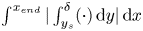 $\int _{}^{x_{end}} |\int _{y_s}^{\delta } (\cdot )\,{\textrm {d}y}|\,{\textrm {d}x}$, respectively. In both the subsonic and supersonic regions across synchronization, the cumulative total perturbation kinetic energy of the initially unstable modes (mode S for
 $M=4.5$ and mode F for
 $M=5.5$) exchanged by pressure–dilatation is negative, whereas the cumulative temperature perturbation energy is positive. Namely, unstable modes experience a reduction of kinetic energy while being heated. The linearized pressure–dilatation being driven by the perturbation–dilatation (
 $(p \theta )_L \approx \bar p \hat \theta$), pressure and temperature perturbations are in the same relation as the perturbation–dilatation. For the initially stable modes, in the supersonic region an increase of kinetic energy by dilatation effects is not accompanied by a reversible decrease of temperature perturbation energy, and pressure and temperature perturbations are not in the same relation as the perturbation–dilatation. In the subsonic region, as is the case of the initially unstable modes, they experience a reduction of kinetic energy while being heated. Furthermore, the energy transfer process occurs in the early stages of the evolution and is completed before synchronization location. Table 2 summarizes the results for all Mach numbers and it shows that the energy exchanges exhibit the same features, independently of the Mach number and of the wall thermal conditions.
Streamwise distributions of the cumulative total perturbation kinetic energy ( ${\mathcal {I}}_{p\theta }$) and temperature perturbation energy (
 ${\mathcal {I}}_{-T(p \theta )_L}$) of modes S and F exchanged through dilatation in the subsonic (superscript ‘
 $sub$’) and supersonic (superscript ‘
 $sup$’) regions. In the subsonic and supersonic regions, the rates are normalized, respectively, by
 $\int _{}^{x_{end}} |\int _{0}^{y_s} (\cdot ) \,{\textrm {d}y}| \,{\textrm {d}x}$ and
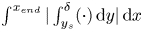 $\int _{}^{x_{end}} |\int _{y_s}^{\delta } (\cdot )\,{\textrm {d}y}|\,{\textrm {d}x}$. Solid line, initially unstable mode; dashed line, initially stable mode. (a)
 $M=4.5$; (b)
 $M=5.5$.

Cumulative total energy due to dilatational effects exchanged through self-interaction at synchronization location in the subsonic and supersonic regions at various Mach numbers. Bold indicates initially unstable mode. Here  $\textit {I}$ means that
 $\hat p$ and
 $\hat T$ are in phase, whereas
 $\textit {O}$ means that
 $\hat p$ and
 $\hat T$ are not in phase.

To further highlight the minor role of cross-interactions, we report in figure 20 the streamwise distributions of the cumulative total perturbation kinetic energy ( ${\mathcal {I}}_{p\theta }$) and temperature perturbation energy (
 ${\mathcal {I}}_{-T(p\theta )_L}$) exchanged by cross-interaction (S/F and F/S as defined in § 4.2.4) through dilatation. The results show that the energy exchanges exhibit the same features of self-interactions, independently of the Mach number and of the wall thermal conditions.
Initially unstable/initially stable mode interactions. Streamwise distributions of the cumulative total perturbation kinetic energy ( ${\mathcal {I}}_{p\theta }$) and temperature perturbation energy (
 ${\mathcal {I}}_{-T(p\theta )_L}$) exchanged by cross-interaction (S/F and F/S) through dilatation in the subsonic (superscript ‘
 $sub$’) and supersonic (superscript ‘
 $sup$’) regions. In the subsonic and supersonic regions the rates are normalized, respectively, by
 $\int _{}^{x_{end}} |\int _{0}^{y_s} (\cdot )\,{\textrm {d}y}| \,{\textrm {d}x}$ and
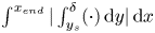 $\int _{}^{x_{end}} |\int _{y_s}^{\delta } (\cdot )\,{\textrm {d}y}|\,{\textrm {d}x}$ of the corresponding direct-interaction terms (S/S and F/F, respectively). (a)
 $M=4.5$, S/F; (b)
 $M=5.5$, F/S; (c)
 $M=6$, S/F; (d)
 $M=6.5$, S/F.

7. Conclusions
In the present study we have carried out an analysis of the energy exchange mechanisms driving the evolution of the leading perturbation modes at hypersonic Mach number for both adiabatic and cold-wall thermal conditions. The analysis focusing on the early stages of laminar-to-turbulent transition, we have developed a weakly nonlinear formulation of the hypersonic boundary-layer stability following the work of Chu & Kovasznay (Reference Chu and Kovasznay1958).
The selected conditions of the adiabatic wall cases are those of Ma & Zhong (Reference Ma and Zhong2003a) and Reed & Balakumar (Reference Reed and Balakumar1990) for  $M=4.5$ and
 $M=6$, respectively, whereas for the cold-wall cases they are those of Fedorov & Tumin (Reference Fedorov and Tumin2011) at
 $M=5.5$ and
 $M=6.5$. Linear stability theory shows that all selected cases exhibit synchronization of the slow (S) and fast (F) modes, and are all inviscidly unstable. For the adiabatic cases and for the
 $M=6.5$ cold-wall case, mode S is initially unstable, whereas mode F is the initially unstable one at
 $M=5.5$.
A detailed scrutiny of the budgets of the various perturbation variables, including the perturbation entropy, the perturbation kinetic energy and the temperature perturbation energy, has led us to conclude that there is no dominant physical mechanism leading to synchronization and that the nature of the energy transfer process is essentially inviscid. Perturbation kinetic energy and temperature perturbation energy are reversibly exchanged through perturbation–dilatational effects, the exchanges associated with those due to base flow dilatation being negligible.
The energy transfer mechanism is driven by the initially unstable modes, and their synchronization with the initially stable modes is not the result of any particular mechanism that takes over. The subsonic layer is the region where the energy transfer mechanism is primarily seeded as a consequence of the thermoacoustic trapping. In this region, the analysis shows that the pressure and temperature perturbations (at any order) are in the same relation as the perturbation–dilatation (of the same order). As a result, when  $p$ and
 $\theta$ are in phase,
 $T$ and
 $\theta$ are also in phase and perturbation kinetic energy is produced at the expense of temperature perturbation energy. The opposite is true when
 $p$ and
 $\theta$ are not in phase.
The direction of the conversion process associated with  $p\theta$ is determined by the sign of the phase difference between the pressure and the dilatation. The phase difference (
 $\varphi _p-\varphi _{\theta }$) features a nearly sinusoidal variation in the streamwise direction alternating between positive and negative values, exhibiting sign changes also in the wall-normal direction in the subsonic region. This indicates that a two-way reversible energy transfer process is established alternating between cooling and heating, in both the streamwise and wall-normal directions. This behaviour is observed only when accounting for second-order contributions, thus confirming the essential role of nonlinear effects in the phase change of the pressure–dilatation.
In the subsonic layer, the thermal power dissipation due to heat conduction is strongly affected by the wall thermal conditions, and is more significant for cold wall due to reduction of the boundary-layer scales and the subsequent increase of both the mean and perturbation temperature gradients. In the supersonic region, the large gradients that establish at the critical layer height account for significant thermal power dissipation independently of the wall thermal state.
In conclusion, the present study indicates that the spatial evolution of both slow and fast modes is driven by the same dilatational mechanisms. The analysis of the amplitudes of the nonlinear contributions for both self- and cross-interactions of first-order velocity and temperature modes shows that no significant changes occur as the modes evolve in the streamwise direction when crossing the synchronization location, and this for both self- and cross-interactions. In addition, we also observe that the energy exchanges exhibit the same features of self-interactions, independently of the Mach number and of the wall thermal conditions. This result is consistent with PSE and DNS analyses that observe only the unstable mode (hence, no cross-interaction). Another possibility to further investigate the absence of FS synchronization at various Mach numbers and wall thermal conditions might be to use an input/output methodology, where modes F and S could be prescribed as inputs, and the output response could rely on DNS or nonlinear PSE solver, rather than the linearized Navier–Stokes solver in Nichols & Candler (Reference Nichols and Candler2019).
Supplementary material
Supplementary material is available at https://doi.org/10.1017/jfm.2024.912.
Acknowledgements
The first author acknowledges funding received from Princeton University as Global Research Scholar and William Robert Kenan, Jr., Distinguished Visiting Professor in the Department of Mechanical and Aerospace Engineering of the School of Engineering and Applied Science. He also acknowledges fruitful exchanges on the subject with Professor H. A. Stone.
Declaration of interests
The authors report no conflict of interest.
Data availability statement
The data that support the findings of this study are available on request.
Appendix A. Governing equations for the base flow properties
A.1. Base flow equations
The governing equations for the base flow are derived assuming two-dimensional (quasi-)non-parallel base flow, namely  ${\bar u}={\bar u}(x,y), {\bar v}={\bar v}(x,y),{\bar w}=0, {\bar \rho }={\bar \rho }(x,y), {\bar T}={\bar T}(x,y), {\bar p}={\bar p}(x,y)$. In non-divergence form, the governing equations (2.1a)–(2.1c) for the base flow variables (
 ${\bar \rho },{\bar u},{\bar v},{\bar p},{\bar T}$) reduce to
 $$\begin{gather} {\bar u}\frac{\partial{\bar \rho}}{\partial x} + {\bar v}\frac{\partial{\bar \rho}}{\partial y} +{\bar \rho}\frac{\partial{\bar u}}{\partial x} + {\bar \rho}\frac{\partial{\bar v}}{\partial y} = 0, \end{gather}$$
 $$\begin{gather}{\bar u}\frac{\partial{\bar u}}{\partial x} + {\bar v}\frac{\partial{\bar u}}{\partial y} ={-} \frac{1}{{\bar \rho}}\frac{\partial {\bar p}}{\partial x }+D_{\bar u}, \end{gather}$$
 $$\begin{gather}{\bar u}\frac{\partial{\bar v}}{\partial x} + {\bar v}\frac{\partial{\bar v}}{\partial y} ={-} \frac{1}{{\bar \rho}}\frac{\partial {\bar p}}{\partial y }+ D_{\bar v}, \end{gather}$$
 $$\begin{gather}{\bar u}\frac{\partial{\bar T}}{\partial x} + {\bar v}\frac{\partial{\bar T}}{\partial y} ={-}\frac{\bar p}{{\bar \rho}c_v} \left(\frac{\partial \bar u}{\partial x }+\frac{\partial \bar v}{\partial y }\right)+D_{\bar T}+\phi_{\bar T}, \end{gather}$$
 $$\begin{gather}{\bar p}={\bar \rho}R{\bar T}, \end{gather}$$
with
 \begin{gather}\begin{aligned}[b] D_{\bar u}
&= {\bar \nu}\frac{\partial}{\partial
x}{\left[2\frac{\partial {\bar u}}{\partial x}-
\frac{2}{3}\left(\frac{\partial {\bar u}}{\partial x
}+\frac{\partial {\bar v}}{\partial y }\right) \right]}+
{\bar \nu} \frac{\partial}{\partial y }
\left(\frac{\partial {\bar u}}{\partial y }+\frac{\partial
{\bar v}}{\partial x }\right) \nonumber\\ &\quad
+\frac{1}{{\bar \rho}}\left[ 2\frac{\partial {\bar
u}}{\partial x}- \frac{2}{3}\left(\frac{\partial {\bar
u}}{\partial x }+\frac{\partial {\bar v}}{\partial
y}\right)\right] \frac{\partial {\bar \mu}}{\partial x
}+\frac{1}{{\bar \rho}}\left(\frac{\partial {\bar
u}}{\partial y }+ \frac{\partial {\bar v}}{\partial x
}\right)\frac{\partial {\bar \mu}}{\partial y},\end{aligned}
\end{gather}
 \begin{gather}
\begin{aligned}[b] D_{\bar v} &= {\bar \nu}
\frac{\partial}{\partial x } \left(\frac{\partial {\bar
u}}{\partial y }+ \frac{\partial {\bar v}}{\partial x
}\right)+{\bar \nu} \frac{\partial}{\partial
y}{\left[2\frac{\partial {\bar v}}{\partial y}-
\frac{2}{3}\left(\frac{\partial {\bar u}}{\partial x }+
\frac{\partial {\bar v}}{\partial y }\right)\right]}
\nonumber\\ &\quad +\frac{1}{{\bar
\rho}}\left(\frac{\partial {\bar u}}{\partial y }+
\frac{\partial {\bar v}}{\partial x }\right)\frac{\partial
{\bar \mu}}{\partial x }+ \frac{1}{{\bar \rho}}\left[
2\frac{\partial {\bar v}}{\partial y}-
\frac{2}{3}\left(\frac{\partial {\bar u}}{\partial x
}+\frac{\partial {\bar v}}{\partial y}\right)\right]
\frac{\partial {\bar \mu}}{\partial y},\end{aligned}
\end{gather}
 \begin{gather} \left.\begin{gathered} D_{\bar T} = \frac{\gamma}{Pr} \nu \left(\frac{\partial^2 {\bar T}}{\partial^2 x}+ \frac{\partial^2 {\bar T}}{\partial^2 y}\right) +\frac{\gamma}{Pr} \left(\frac{\partial {\bar T}}{\partial x }\frac{\partial {\bar \mu}}{\partial x }+ \frac{\partial {\bar T}}{\partial y }\frac{\partial {\bar \mu}}{\partial y }\right), \\ \phi_{\bar T}=\frac{1}{c_v} {\bar \phi}, \end{gathered}\right\} \end{gather}
with  ${\bar \phi }$ the viscous dissipation of base flow kinetic energy (
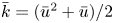 ${\bar k}=({\bar u}^2+{\bar u})/2$):
 \begin{equation} {\bar \phi}={\bar \nu}\left[2 \left(\frac{\partial \bar u}{\partial x}\right)^2+ 2 \left(\frac{\partial \bar v}{\partial y }\right)^2+ \left(\frac{\partial \bar u}{\partial y }+\frac{\partial \bar v}{\partial x }\right)^2- \frac{2}{3}\left(\frac{\partial \bar u}{\partial x }+\frac{\partial \bar v}{\partial y}\right)^2\right], \end{equation}
and  $D_{\bar u}$,
 $D_{\bar v}$ and
 $D_{\bar T}$ and
 $\bar \phi$ represent, respectively, the diffusion of the streamwise and wall-normal velocities and the exchange of the base flow internal energy by heat conduction.
The governing equations for the base flow entropy and energy variables are given as follows:
 $$\begin{gather} {\bar u}\frac{\partial{\bar s}}{\partial x} + {\bar v}\frac{\partial{\bar s}}{\partial y} = D_{\bar s}+\phi_{\bar s,\bar u}+\phi_{\bar s,\bar T}, \end{gather}$$
 $$\begin{gather}{\bar u}\frac{\partial{\bar k}}{\partial x} + {\bar v}\frac{\partial{\bar k}}{\partial y} ={-}\frac{1}{\bar \rho}{ \varPi}_{\bar W}+\frac{1}{\bar \rho}{\varPi}_{\bar \theta}+D_{\bar k}-{\bar \phi}, \end{gather}$$
 $$\begin{gather}{\bar u}\frac{\partial{\bar k_T}}{\partial x} + {\bar v}\frac{\partial{\bar k_T}}{\partial y} ={-}\frac{1}{\bar \rho}\varPi_{\bar \theta,\bar T}+D_{\bar k_T}+{\bar \phi_u}-{\bar \phi_{k_T}}, \end{gather}$$
where  ${\bar k_T}={\bar T}^2/2$ is the base flow ‘temperature’ energy variable.
The terms  $D_{\bar s}$,
 $\phi _{\bar s,\bar u}$ and
 $\phi _{\bar s,\bar T}$ appearing in (A10) stand for, respectively, the diffusion of base flow entropy associated with heat conduction, and the generation rates due to viscous and thermal power dissipation:
 \begin{equation} \left.\begin{gathered} D_{\bar s}=\frac{\nu}{Pr}\left[\frac{\partial}{\partial x}\left(\frac {1}{\bar T} \frac{\partial {\bar T}}{\partial x}\right) +\frac{\partial}{\partial y}\left(\frac {1}{\bar T} \frac{\partial {\bar T}}{\partial y}\right)\right] +\frac{1}{Pr}\frac{1}{\bar \rho} \left(\frac{\partial {\bar T}}{\partial x } \frac{\partial {\bar \mu}}{\partial x }+ \frac{\partial {\bar T}}{\partial y }\frac{\partial {\bar \mu}}{\partial y }\right),\\ \phi_{\bar s,\bar u}=\frac{1}{c_p}\frac {1}{\bar T} \bar \phi,\\ \phi_{\bar s,\bar T}=\frac{\nu}{Pr}\left[\left(\frac {1}{\bar T} \frac{\partial {\bar T}}{\partial x}\right)^2+\left(\frac {1}{\bar T} \frac{\partial {\bar T}}{\partial y}\right)^2\right].\end{gathered}\right\} \end{equation}
The terms  ${ \varPi }_{\bar W}$,
 ${\varPi }_{\bar \theta }$,
 $D_{\bar k}$ and
 ${\bar \phi }$ of (A11) represent, respectively, the pressure work, the pressure–dilatation, the diffusion of the base flow kinetic energy and its dissipation due to viscous effects:
 $$\begin{gather} {\varPi}_{\bar W}=\left(\frac{\partial {\bar u \bar p}}{\partial x }+ \frac{\partial {\bar v \bar p}}{\partial y }\right), \end{gather}$$
 $$\begin{gather}{\varPi}_{\bar \theta}={\bar p}\left(\frac{\partial {\bar u}}{\partial x }+ \frac{\partial {\bar v}}{\partial y }\right), \end{gather}$$
 \begin{gather}\begin{aligned}[b] D_{\bar k} &= {\bar \nu}\frac{\partial}{\partial x }{\bar u \left[2\frac{\partial {\bar u}}{\partial x}- \frac{2}{3}\left(\frac{\partial {\bar u}}{\partial x }+ \frac{\partial {\bar v}}{\partial y }\right) \right]}+ {\bar \nu} \frac{\partial}{\partial y } \left[\bar u \left(\frac{\partial {\bar u}}{\partial y }+ \frac{\partial {\bar v}}{\partial x }\right)\right] \nonumber\\ &\quad +\frac{1}{{\bar \rho}}\bar u \left[ 2\frac{\partial {\bar u}}{\partial x}- \frac{2}{3}\left(\frac{\partial {\bar u}}{\partial x }+\frac{\partial {\bar v}}{\partial y }\right)\right] \frac{\partial {\bar \mu}}{\partial x }+\frac{1}{{\bar \rho}}\bar u\left(\frac{\partial {\bar u}}{\partial y }+ \frac{\partial {\bar v}}{\partial x }\right)\frac{\partial {\bar \mu}}{\partial y } \nonumber\\ &\quad +{\bar \nu} \frac{\partial}{\partial x } \left[\bar v \left(\frac{\partial {\bar u}}{\partial y }+ \frac{\partial {\bar v}}{\partial x }\right)\right] \nonumber\\ &\quad +\frac{1}{\bar \rho}\bar v \left(\frac{\partial {\bar u}}{\partial y }+ \frac{\partial {\bar v}}{\partial x }\right)\frac{\partial {\bar \mu}}{\partial x } +{\bar \nu}\frac{\partial}{\partial y }{\bar v\left[ 2\frac{\partial {\bar v}}{\partial y}- \frac{2}{3}\left(\frac{\partial {\bar u}}{\partial x }+\frac{\partial {\bar v}}{\partial y }\right)\right]} \nonumber\\ &\quad +\frac{1}{{\bar \rho}}\bar v \left[ 2\frac{\partial {\bar v}}{\partial y}- \frac{2}{3}\left(\frac{\partial {\bar u}}{\partial x }+\frac{\partial {\bar v}}{\partial y }\right)\right] \frac{\partial {\bar \mu}}{\partial y }.\end{aligned} \end{gather}
Terms  $\varPi _{\bar \theta,\bar T}$,
 $D_{\bar k_T}$,
 ${\bar \phi _u}={\bar T}{\bar \phi }$ and
 ${\bar \phi _{k_T}}$ stand for, respectively, the base flow temperature/pressure–dilatation, the diffusion of the base flow energy variable and its production due to the action of the base flow viscous forces and the thermal power dissipation associated with base flow heat conduction.:
 $$\begin{gather} \varPi_{\bar \theta,\bar T}= {\bar T}{\bar p}\left(\frac{\partial {\bar u}}{\partial x }+\frac{\partial {\bar v}}{\partial y }\right), \end{gather}$$
 $$\begin{gather}D_{\bar k_T}= \frac{\gamma}{Pr}\nu \left(\frac{{\partial}^2 {\bar k_T}}{\partial x^2} + \frac{{\partial}^2 {\bar k_T}}{\partial y^2}\right) + \frac{\gamma}{Pr}\frac{1}{\bar \rho}\left(\frac{\partial{\bar k_T}}{\partial x}\frac{\partial {\bar \mu}}{\partial x }+ \frac{\partial{\bar k_T}}{\partial y}\frac{\partial {\bar \mu}}{\partial y }\right), \end{gather}$$
 $$\begin{gather}{\bar \phi_u}= \frac{\gamma}{c_v} {\bar T}{\bar \phi}, \end{gather}$$
 $$\begin{gather}{\bar \phi_{k_T}}= \frac{1}{c_v} \bar \nu\left[ \left(\frac{\partial {\bar T}}{\partial x}\right)^2+\left(\frac{\partial {\bar T}}{\partial y}\right)^2 \right]. \end{gather}$$
A.2. Base flow analysis
The solution of the base flow equations (A1)–(A4) is obtained through the similarity solution of a zero-pressure-gradient compressible laminar boundary layer and introducing a generalized coordinate transformation based on the Lees–Dorodnitsyn similarity variables (Anderson Reference Anderson2002), with the streamwise derivatives appearing in the equations being evaluated by finite differencing. In figure 21 (only the  $M=4.5$ adiabatic wall case is reported), we briefly discuss the budgets of the base flow streamwise velocity component (
 ${\bar u}$), entropy (
 ${\bar s}$), kinetic energy (
 ${\bar k}$) and ‘temperature’ energy (
 ${\bar k_T}$). In the critical-layer region, the streamwise convection of
 ${\bar u}$
 $(\bar u ({\partial \bar u }/{\partial x}))$ is affected by diffusion and convection normal to the wall
 $(\bar v ({\partial \bar u }/{\partial y}))$, which depend strongly on the large gradients that establish in this region. Base flow entropy is produced primarily by thermal power due to heat conduction that is then diffused towards the wall balancing entropy production by viscous dissipation. Similarly, in the region around the critical layer, base flow kinetic energy is produced and it diffuses towards the wall balancing the energy removed by viscous dissipation, whereas
 ${\bar k_T}$ is removed by thermal power dissipation and diffused by heat conduction towards the wall to balance the production due to viscous dissipation.
Base flow budgets at  $M=4.5$. The symbols on the vertical axes identify the locations of the sonic and critical layer heights for the slow and fast modes: square, generalized inflection point; diamond, critical layer height; circle, sonic layer height.

Appendix B. Linear stability matrices
Dropping the superscripts  $()^{\prime }$ and
 $()^{\prime \prime }$ and decomposing the disturbances in normal modes, the stability equations are cast in the following compact matrix form:
 \begin{equation} \boldsymbol{\mathsf{C}}\frac{{\rm d}^2 \hat{\boldsymbol{q}}}{{{\rm d}y}^2 }+\boldsymbol{\mathsf{B}}\frac{{\rm d} \hat{\boldsymbol{q}}}{{{\rm d}y}}+\boldsymbol{\mathsf{A}}{\hat{\boldsymbol{q}}}=(n-1) f {\skew2\hat{\boldsymbol{\mathsf{N}}}}, \end{equation}
where  $\boldsymbol{\mathsf{A}}=\boldsymbol{\mathsf{A}}(\alpha,\omega,M,Re; {\bar \rho },{\bar u_i},{\bar p},{\bar T})$,
 $\boldsymbol{\mathsf{B}}=\boldsymbol{\mathsf{B}}(\alpha,\omega,M,Re; {\bar \rho },{\bar u_i},{\bar p},{\bar T})$ and
 $\boldsymbol{\mathsf{C}}=\boldsymbol{\mathsf{C}}(\alpha,\omega, M,Re; {\bar \rho },{\bar u_i},{\bar p},{\bar T})$ are (
 $5 \times 5$) matrices (we recall that
 ${\hat {\boldsymbol{\mathsf{N}}}}$ is the normal-mode representation of the first-order interaction contribution to the second-order modes). The non-zero coefficients of
 $\boldsymbol{\mathsf{A}}$,
 $\boldsymbol{\mathsf{B}}$ and
 $\boldsymbol{\mathsf{C}}$ are
 $$\begin{gather} A_{1,1}= \left({\rm i} \bar \rho \alpha+\frac{\partial {\bar \rho}}{\partial x} \right), \end{gather}$$
 $$\begin{gather}A_{1,2}=\frac{\partial {\bar \rho}}{\partial y}, \end{gather}$$
 $$\begin{gather}A_{1,4}= \left\{ \left[{\rm i} \left(\alpha {\bar u}-\omega \right)+ \left(\frac{\partial {\bar u}}{\partial x }+\frac{\partial {\bar v}}{\partial y } \right) \right]\frac{\bar \rho}{\bar p}+ {\bar u} \left(\frac{1}{\bar p}\frac{\partial {\bar \rho}}{\partial x}-\frac{\bar \rho}{{\bar p}^2}\frac{\partial {\bar p}}{\partial x} \right)+ {\bar v} \left(\frac{1}{\bar p}\frac{\partial {\bar \rho}}{\partial y}-\frac{\bar \rho}{{\bar p}^2}\frac{\partial {\bar p}}{\partial y} \right) \right\}, \end{gather}$$
 \begin{gather}\begin{aligned}[b] A_{1,5} &={-} \left\{\left[{\rm i} \left(\alpha {\bar u}-\omega \right)+\left(\frac{\partial {\bar u}}{\partial x }+\frac{\partial {\bar v}}{\partial y } \right) \right]\frac{\bar \rho}{\bar T}+ {\bar u} \left(\frac{1}{\bar T}\frac{\partial {\bar \rho}}{\partial x}-\frac{\bar \rho}{{\bar T}^2}\frac{\partial {\bar T}}{\partial x} \right) \right.\nonumber\\ &\quad \left.+\,{\bar v} \left(\frac{1}{\bar T}\frac{\partial {\bar \rho}}{\partial y}- \frac{\bar \rho}{{\bar T}^2}\frac{\partial {\bar T}}{\partial y} \right) \right\},\end{aligned}\end{gather}
 $$\begin{gather} A_{2,1}= \left\{ \left[{\rm i} \left(\alpha {\bar u}-\omega \right)+\frac{\partial {\bar u}}{\partial x } \right] {\bar \rho}+\frac{4}{3}{\bar \mu} \left(\alpha^2-{\rm i}\frac{{\rm d} \alpha}{{\rm d}\kern 0.06em x} \right) -\frac{4}{3}{\rm i}\alpha\frac{\partial {\bar \mu}}{\partial x} \right\}, \end{gather}$$
 $$\begin{gather}A_{2,2}= \left({\bar \rho}\frac{\partial \bar u}{\partial y}-{\rm i}\alpha\frac{\partial {\bar \mu}}{\partial y} \right), \end{gather}$$
 $$\begin{gather}A_{2,4}= \left[ \left(\bar u\frac{\partial {\bar u}}{\partial x }+\bar v \frac{\partial {\bar u}}{\partial y } \right)\frac{\bar \rho}{\bar p}+{\rm i}\alpha \right], \end{gather}$$
 $$\begin{gather}A_{2,5}={-} \left(\bar u\frac{\partial {\bar u}}{\partial x }+\bar v \frac{\partial {\bar u}}{\partial y } \right)\frac{\bar \rho}{\bar T}, \end{gather}$$
 $$\begin{gather}A_{3,1}= \left({\bar \rho}\frac{\partial {\bar v}}{\partial x }+\frac{2}{3}{\rm i}\alpha\frac{\partial {\bar \mu}}{\partial y } \right), \end{gather}$$
 $$\begin{gather}A_{3,2}= \left[{\rm i} \left(\alpha {\bar u}-\omega \right)+\frac{\partial {\bar v}}{\partial y } \right]{\bar \rho}+{\bar \mu} \left(\alpha^2-{\rm i}\frac{{\rm d} \alpha}{{\rm d}\kern 0.06em x} \right)-{\rm i}\alpha\frac{\partial {\bar \mu}}{\partial x }, \end{gather}$$
 $$\begin{gather}A_{3,4}= \left[ \left(\bar u\frac{\partial {\bar v}}{\partial x }+\bar v \frac{\partial {\bar v}}{\partial y } \right)\frac{\bar \rho}{\bar p} \right], \end{gather}$$
 $$\begin{gather}A_{3,5}={-} \left(\bar u\frac{\partial {\bar v}}{\partial x }+\bar v \frac{\partial {\bar v}}{\partial y } \right)\frac{\bar \rho}{\bar T}, \end{gather}$$
 $$\begin{gather}A_{4,3}= \left\{ {\rm i} \left(\alpha {\bar u}-\omega \right){\bar \rho}+ \left[{\bar \mu} \left(\alpha^2-{\rm i}\frac{{\rm d} \alpha}{{\rm d}\kern 0.06em x} \right)-{\rm i}\alpha\frac{\partial {\bar \mu}}{\partial x } \right]\right\}, \end{gather}$$
 $$\begin{gather}A_{5,1}= \left\{{\bar \rho}\frac{\partial {\bar T}}{\partial x }+{\rm i}\alpha\frac{\bar p}{c_v}- {\rm i}\alpha\frac{\bar \mu}{c_v} \left[ 4\frac{\partial \bar u}{\partial x } -\frac{4}{3}\left(\frac{\partial \bar u}{\partial x }+\frac{\partial \bar v}{\partial y } \right)\right]\right\}, \end{gather}$$
 $$\begin{gather}A_{5,2}= \left[{\bar \rho}\frac{\partial {\bar T}}{\partial y }-{\rm i}\alpha \frac{\bar \mu}{c_v} 2 \left(\frac{\partial \bar u}{\partial y }+\frac{\partial \bar v}{\partial x } \right) \right], \end{gather}$$
 $$\begin{gather}A_{5,4}= \left[ \left({\bar u}\frac{\partial {\bar T}}{\partial x }+{\bar v}\frac{\partial {\bar T}}{\partial y } \right)\frac{\bar \rho}{\bar p} +\frac{1}{c_v} \left(\frac{\partial \bar u}{\partial x }+\frac{\partial \bar v}{\partial y } \right) \right], \end{gather}$$
 $$\begin{gather}A_{5,5}= \left\{ {\rm i} \left(\alpha {\bar u}-\omega \right){\bar \rho}- \left({\bar u}\frac{\partial {\bar T}}{\partial x }+{\bar v}\frac{\partial {\bar T}}{\partial y } \right)\frac{\bar \rho}{\bar p}+ \frac{\gamma}{Pr}{\bar \mu} \left(\alpha^2-{\rm i}\frac{{\rm d} \alpha}{{\rm d}\kern 0.06em x} \right)- {\rm i}\alpha \frac{\gamma}{Pr}\frac{\partial {\bar \mu}}{\partial x } \right\}; \end{gather}$$
 $$\begin{gather} B_{1,2}={\bar \rho}, \end{gather}$$
 $$\begin{gather}B_{1,4}={\bar v}\frac{\bar \rho}{\bar p}, \end{gather}$$
 $$\begin{gather}B_{1,5}={-}{\bar v}\frac{\bar \rho}{\bar T}, B_{2,1}= \left({\bar \rho}{\bar v}- \frac{\partial {\bar \mu}}{\partial y } \right), \end{gather}$$
 $$\begin{gather}B_{2,2}= \left(-{\rm i}\alpha \frac{1}{3} {\bar \mu}+\frac{2}{3}\frac{\partial {\bar \mu}}{\partial x } \right), \end{gather}$$
 $$\begin{gather}B_{3,1}= \left(-{\rm i}\frac{1}{3}\alpha{\bar \mu}-\frac{\partial {\bar \mu}}{\partial x } \right), \end{gather}$$
 $$\begin{gather}B_{3,2}= \left({\bar \rho}{\bar v}-\frac{4}{3}\frac{\partial {\bar \mu}}{\partial y } \right), \end{gather}$$
 $$\begin{gather}B_{3,4}=1, \end{gather}$$
 $$\begin{gather}B_{4,3}= \left({\bar \rho} {\bar v}-\frac{\partial {\bar \mu}}{\partial y } \right), \end{gather}$$
 $$\begin{gather}B_{5,1}={-}\frac{\bar \mu}{c_v}2 \left(\frac{\partial \bar u}{\partial y }+ \frac{\partial \bar v}{\partial x } \right), \end{gather}$$
 $$\begin{gather}B_{5,2}= \left\{\frac{\bar p}{c_v} - \frac{\bar \mu}{c_v} \left[4 \frac{\partial \bar v}{\partial y } - \frac{4}{3} \left(\frac{\partial \bar u}{\partial x }+\frac{\partial \bar v}{\partial y } \right)\right]\right\}, \end{gather}$$
 $$\begin{gather}B_{5,5}= \left({\bar \rho} {\bar v}-\frac{\gamma}{Pr}\frac{\partial \bar \mu}{\partial y } \right); \end{gather}$$
 $$\begin{gather} C_{2,1}={-}{\bar \mu}, \end{gather}$$
 $$\begin{gather}C_{3,2}={-}\frac{4}{3}{\bar \mu}, \end{gather}$$
 $$\begin{gather}C_{4,3}={-}{\bar \mu}, \end{gather}$$
 $$\begin{gather}C_{5,5}={-}\frac{\gamma}{Pr}{\bar \mu}. \end{gather}$$



