1. Introduction
It is well known that the addition of three-dimensional (3D) spanwise-periodic perturbations to a two-dimensional (2D) cylinder wake can stabilise vortex shedding (Zdravkovich Reference Zdravkovich1981; Kim & Choi Reference Kim and Choi2005; Choi, Jeon & Kim Reference Choi, Jeon and Kim2008). Recently, Hwang, Kim & Choi (Reference Hwang, Kim and Choi2013) proposed an explanation of this effect based on the linear stability of the spanwise-modulated parallel wake flow. They demonstrated a substantial attenuation of the absolute instability growth rate in a range of wavelengths corresponding to results from experiment and direct numerical simulation.
In a recent paper, Del Guercio, Cossu & Pujals (Reference Del Guercio, Cossu and Pujals2014) showed that suitable spanwise-periodic perturbations added to nominally parallel wakes significantly reduce the temporal stability growth rate of the inflectional instability and completely quench the absolute instability as well. Perturbations to the nominally parallel base flow were chosen as nonlinear streaks resulting from the optimal lift-up mechanism, i.e. the transient growth of optimal streamwise-uniform spanwise-periodic vortices. The absolute and maximum temporal growth rates were found to depend quadratically on the streak amplitudes, as suggested by Hwang et al. (Reference Hwang, Kim and Choi2013), who demonstrated that the linear sensitivity was zero for spanwise-periodic disturbances of the base flow.
Cossu (Reference Cossu2014) outlined a rigorous mathematical procedure to compute beforehand the quadratic (second-order) sensitivity of an eigenmode when its linear (first-order) sensitivity vanishes. He used this method to explain the stabilisation of global modes of the one-dimensional (1D) Ginzburg–Landau equation, serving as a model equation for spatially developing shear flows submitted to spanwise-periodic modulations. Tammisola et al. (Reference Tammisola, Giannetti, Citro and Juniper2014) applied a similar technique to investigate the stabilisation of the 2D wake behind a flat plate using spanwise-periodic wall actuation. In these two studies, particular base flow modifications were prescribed and the resulting first-order eigenmode variation had to be computed explicitly to obtain the eigenvalue variation.
In this paper, we address the question of optimal spanwise-periodic flow modification. In a first step, we use an asymptotic expansion to express the second-order eigenvalue variation, and we determine a second-order sensitivity operator which allows us to predict the eigenvalue variation resulting from any base flow modification without ever computing the first-order eigenmode correction and without solving the modified eigenvalue problem. Then, we optimise the eigenvalue variation and obtain optimal flow modifications, i.e. the optimally destabilising/stabilising spanwise-periodic base flow modulations. We illustrate this optimisation technique with the classical hydrodynamic stability of nominally parallel flows governed by the linearised Navier–Stokes equations at finite Reynolds number
 $\mathit{Re}$
(the so-called Orr–Sommerfeld equations) in the unstable regime: the plane channel flow and a prototypical mixing layer. A normal mode expansion yields a set of eigenvalues and eigenmodes for any given streamwise and spanwise wavenumbers
 $({\it\alpha}_{0},{\it\beta}_{0})$
, and in both flows the most unstable mode is two-dimensional (
 ${\it\beta}_{0}=0$
). We consider base flow modifications that are unidirectional and parallel to the base flow direction, and spanwise-periodic of wavenumber
 ${\it\beta}$
. For each wavenumber pair
 $({\it\alpha}_{0},{\it\beta})$
, we optimise the variation of the leading 2D eigenvalue, thus obtaining bounds for this variation together with the associated optimally destabilising/stabilising base flow modifications. The effect on other modes
 $({\it\alpha}_{0},{\it\beta}_{0})$
is also discussed.
In a second step, we incorporate transient growth in the optimisation procedure and find combined optimal perturbations that achieve the best trade-off between transient amplification and stabilisation. Indeed, flow modifications optimised for pure stabilisation do not take advantage of non-normal amplification mechanisms and may thus require a substantial amplitude; on the other hand, perturbations optimised for pure transient growth may not be well suited to stabilisation. This combined optimisation is conducted under the strong hypothesis of a separation of time scales between the fast instability of the nominal base flow and the slow evolution of purely transverse steady initial perturbations into streaks (Reddy et al. Reference Reddy, Schmid, Baggett and Henningson1998; Cossu & Brandt Reference Cossu and Brandt2004).
Section 2 details the derivation of the second-order sensitivity operator and the optimisation method. Sections 3 and 4 are devoted to optimal flow modifications in the plane channel flow and in the mixing layer. Section 5 presents the combined optimisation of transient growth and flow modification, and characterises the performance of optimal streaks in different
 ${\it\beta}$
ranges. Comparison of spanwise-uniform and spanwise-periodic optimals is also provided.
2. Problem formulation
Given a steady base flow
 $(\unicode[STIX]{x1D650},P)^{\text{T}}$
solution of the Navier–Stokes (NS) equations, the dynamics of small-amplitude perturbations
 $\hat{\unicode[STIX]{x1D666}}=(\hat{\boldsymbol{u}},\hat{p})^{\text{T}}=(\hat{u} ,\hat{v},{\hat{w}},\hat{p})^{\text{T}}$
superimposed onto this base flow are governed by the linearised NS equations
 $$\begin{eqnarray}\partial _{t}\hat{\boldsymbol{u}}+\unicode[STIX]{x1D650}\boldsymbol{\cdot }\boldsymbol{{\rm\nabla}}\hat{\boldsymbol{u}}+\hat{\boldsymbol{u}}\boldsymbol{\cdot }\boldsymbol{{\rm\nabla}}\unicode[STIX]{x1D650}+\boldsymbol{{\rm\nabla}}\hat{p}-\mathit{Re}^{-1}{\rm\nabla}^{2}\hat{\boldsymbol{u}}=\mathbf{0},\quad \boldsymbol{{\rm\nabla}}\boldsymbol{\cdot }\hat{\boldsymbol{u}}=0.\end{eqnarray}$$
2.1. Second-order eigenvalue variation
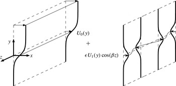
Consider a 1D parallel flow
 $U_{0}(y)\boldsymbol{e}_{x}$
perturbed with a 2D spanwise-periodic modification of small amplitude
 ${\it\epsilon}$
as shown in figure 1:
 $$\begin{eqnarray}\unicode[STIX]{x1D650}(y,z)=(U_{0}(y)+{\it\epsilon}U_{1}(y)\cos ({\it\beta}z))\boldsymbol{e}_{x}.\end{eqnarray}$$
Assuming a normal mode expansion
 $\hat{\unicode[STIX]{x1D666}}(x,y,z,t)=\unicode[STIX]{x1D666}(y,z)\exp (\text{i}{\it\alpha}_{0}x+{\it\lambda}t)$
in spanwise coordinate
 $x$
and time
 $t$
for small-amplitude perturbations and linearising the NS equations results in the eigenvalue problem
 $$\begin{eqnarray}{\it\lambda}\boldsymbol{u}+\unicode[STIX]{x1D650}\boldsymbol{\cdot }\boldsymbol{{\rm\nabla}}\boldsymbol{u}+\boldsymbol{u}\boldsymbol{\cdot }\boldsymbol{{\rm\nabla}}\unicode[STIX]{x1D650}+\boldsymbol{{\rm\nabla}}p-\mathit{Re}^{-1}{\rm\nabla}^{2}\boldsymbol{u}=\mathbf{0},\quad \boldsymbol{{\rm\nabla}}\boldsymbol{\cdot }\boldsymbol{u}=0,\end{eqnarray}$$
for the eigenvalue
 ${\it\lambda}={\it\lambda}_{r}+\text{i}{\it\lambda}_{i}$
. The set of growth rates
 ${\it\lambda}_{r}$
and frequencies
 ${\it\lambda}_{i}$
determines the linear temporal stability properties of the flow.
Sketch of the base flow configuration: a 1D parallel flow
 $U_{0}(y)$
is modified with a small-amplitude 2D spanwise-periodic flow
 ${\it\epsilon}U_{1}(y)\cos ({\it\beta}z)$
.

While it is common at this stage, for spanwise-invariant parallel base flows, to transform the primitive variables
 $\unicode[STIX]{x1D666}=(\boldsymbol{u},p)^{\text{T}}$
into the Orr–Sommerfeld variables (cross-stream velocity and vorticity), we keep here the primitive variables and write (2.3) formally as
 ${\it\lambda}\unicode[STIX]{x1D640}\unicode[STIX]{x1D666}+\unicode[STIX]{x1D63C}\unicode[STIX]{x1D666}=\mathbf{0}$
. Since the linearised NS operator
 $\unicode[STIX]{x1D63C}$
is linear in the base flow
 $\unicode[STIX]{x1D650}$
, it can be expanded exactly to arbitrary order (here to second order) as
 $\unicode[STIX]{x1D63C}=\unicode[STIX]{x1D63C}_{0}+{\it\epsilon}\unicode[STIX]{x1D63C}_{1}$
. The singular matrix
 $\unicode[STIX]{x1D640}$
need not be expanded since it does not depend on the base flow. Detailed expressions for all operators are given in appendix A. It should be noted in particular that
 $\unicode[STIX]{x1D63C}_{0}$
depends on the unperturbed base flow
 $U_{0}$
, and
 $\unicode[STIX]{x1D63C}_{1}$
depends on the base flow modification
 $U_{1}$
.
We look for perturbed eigenvalues and eigenmodes using the following expansion in the amplitude
 ${\it\epsilon}$
of the base flow modification:
 $$\begin{eqnarray}{\it\lambda}={\it\lambda}_{0}+{\it\epsilon}{\it\lambda}_{1}+{\it\epsilon}^{2}{\it\lambda}_{2}+\cdots \,,\quad \unicode[STIX]{x1D666}=\unicode[STIX]{x1D666}_{0}+{\it\epsilon}\unicode[STIX]{x1D666}_{1}+{\it\epsilon}^{2}\unicode[STIX]{x1D666}_{2}+\cdots \,.\end{eqnarray}$$
By substituting (2.4) into (2.3), we recover at leading order (
 ${\it\epsilon}^{0}$
) the linearised NS equations
 $$\begin{eqnarray}{\it\lambda}_{0}\boldsymbol{u}_{0}+\unicode[STIX]{x1D650}_{0}\boldsymbol{\cdot }\boldsymbol{{\rm\nabla}}\boldsymbol{u}_{0}+\boldsymbol{u}_{0}\boldsymbol{\cdot }\boldsymbol{{\rm\nabla}}\unicode[STIX]{x1D650}_{0}+\boldsymbol{{\rm\nabla}}p_{0}-\mathit{Re}^{-1}{\rm\nabla}^{2}\boldsymbol{u}_{0}=\mathbf{0},\quad \boldsymbol{{\rm\nabla}}\boldsymbol{\cdot }\boldsymbol{u}_{0}=0,\end{eqnarray}$$
which we write as an eigenvalue problem for the eigenvalue
 ${\it\lambda}_{0}$
and eigenmode
 $\unicode[STIX]{x1D666}_{0}$
:
 $$\begin{eqnarray}({\it\lambda}_{0}\unicode[STIX]{x1D640}+\unicode[STIX]{x1D63C}_{0})\unicode[STIX]{x1D666}_{0}=\mathbf{0}.\end{eqnarray}$$
In the following, we focus on the leading (most unstable) eigenvalue and its associated eigenmode, which is 2D for inflectional velocity profiles:
 $\partial _{z}\unicode[STIX]{x1D666}_{0}=\mathbf{0},w_{0}=0$
.
At first order (
 ${\it\epsilon}^{1}$
) we obtain
 $$\begin{eqnarray}({\it\lambda}_{0}\unicode[STIX]{x1D640}+\unicode[STIX]{x1D63C}_{0})\unicode[STIX]{x1D666}_{1}+({\it\lambda}_{1}\unicode[STIX]{x1D640}+\unicode[STIX]{x1D63C}_{1})\unicode[STIX]{x1D666}_{0}=\mathbf{0}.\end{eqnarray}$$
We introduce the following 1D and 2D Hermitian inner products:
 $$\begin{eqnarray}\displaystyle \left(\unicode[STIX]{x1D656}\,|\,\unicode[STIX]{x1D657}\right)=\lim _{L_{y}\rightarrow \infty }\int _{-L_{y}/2}^{L_{y}/2}\overline{\unicode[STIX]{x1D656}}\boldsymbol{\cdot }\unicode[STIX]{x1D657}\,\text{d}y,\quad \displaystyle ((\unicode[STIX]{x1D656}\,|\,\unicode[STIX]{x1D657}))=\lim _{L_{z}\rightarrow \infty }\frac{1}{L_{z}}\int _{-L_{z}/2}^{L_{z}/2}\left(\unicode[STIX]{x1D656}\,|\,\unicode[STIX]{x1D657}\right)\text{d}z,\end{eqnarray}$$
where the overbar stands for complex conjugate. For any operator
 $\boldsymbol{N}$
we denote
 $\boldsymbol{N}^{\dagger }$
the adjoint operator such that
 $((\unicode[STIX]{x1D656}\,|\,\boldsymbol{N}\unicode[STIX]{x1D657}))=((\boldsymbol{N}^{\dagger }\unicode[STIX]{x1D656}\,|\,\unicode[STIX]{x1D657}))$
 $\forall \,\unicode[STIX]{x1D656},\unicode[STIX]{x1D657}$
. We obtain the first-order eigenvalue variation
 ${\it\lambda}_{1}$
by projecting (2.7) on the leading adjoint eigenmode
 $\unicode[STIX]{x1D666}_{0}^{\dagger }$
defined by
 $(\overline{{\it\lambda}}_{0}\unicode[STIX]{x1D640}+\unicode[STIX]{x1D63C}_{0}^{\dagger })\unicode[STIX]{x1D666}_{0}^{\dagger }=\mathbf{0}$
and normalised with
 $\left(\unicode[STIX]{x1D666}_{0}^{\dagger }\,|\,\unicode[STIX]{x1D640}\unicode[STIX]{x1D666}_{0}\right)=1$
(Hinch Reference Hinch1991; Trefethen et al.
Reference Trefethen, Trefethen, Reddy and Driscoll1993; Chomaz Reference Chomaz2005; Giannetti & Luchini Reference Giannetti and Luchini2007):
 $$\begin{eqnarray}{\it\lambda}_{1}=-((\unicode[STIX]{x1D666}_{0}^{\dagger }\,|\,\unicode[STIX]{x1D63C}_{1}\unicode[STIX]{x1D666}_{0})).\end{eqnarray}$$
Since
 $\unicode[STIX]{x1D63C}_{1}$
is periodic in
 $z$
, the inner product in (2.9) vanishes and the first-order eigenvalue variation is zero:
 ${\it\lambda}_{1}=0$
. In other words, spanwise-periodic flow modifications have no first-order effect on stability properties (Hwang et al.
Reference Hwang, Kim and Choi2013; Cossu Reference Cossu2014; Del Guercio et al.
Reference Del Guercio, Cossu and Pujals2014). From (2.7), the leading eigenmode variation is
 $\unicode[STIX]{x1D666}_{1}=-({\it\lambda}_{0}\unicode[STIX]{x1D640}+\unicode[STIX]{x1D63C}_{0})^{-1}\unicode[STIX]{x1D63C}_{1}\unicode[STIX]{x1D666}_{0}$
. In this expression, the operator
 $({\it\lambda}_{0}\unicode[STIX]{x1D640}+\unicode[STIX]{x1D63C}_{0})$
is not invertible in general since (2.6) has a non-trivial solution, but the inverse is taken in the subspace orthogonal to
 $\unicode[STIX]{x1D666}_{0}$
, and
 $\unicode[STIX]{x1D666}_{1}$
is defined up to any constant component in the direction of
 $\unicode[STIX]{x1D666}_{0}$
(Hinch Reference Hinch1991). This is made possible by the solvability condition (Fredholm theorem) for (2.7) to be satisfied: the forcing term
 $({\it\lambda}_{0}\unicode[STIX]{x1D640}+\unicode[STIX]{x1D63C}_{1})\unicode[STIX]{x1D666}_{0}=\unicode[STIX]{x1D63C}_{1}\unicode[STIX]{x1D666}_{0}$
is orthogonal to the solution
 $\unicode[STIX]{x1D666}_{0}^{\dagger }$
of the adjoint equation associated with (2.6), as expressed precisely by (2.9).
At second order (
 ${\it\epsilon}^{2}$
) we obtain
 $({\it\lambda}_{0}\unicode[STIX]{x1D640}+\unicode[STIX]{x1D63C}_{0})\unicode[STIX]{x1D666}_{2}+\unicode[STIX]{x1D63C}_{1}\unicode[STIX]{x1D666}_{1}+{\it\lambda}_{2}\unicode[STIX]{x1D640}\unicode[STIX]{x1D666}_{0}=\mathbf{0},$
which yields after projection on the leading adjoint eigenmode
 $$\begin{eqnarray}{\it\lambda}_{2}=-((\unicode[STIX]{x1D666}_{0}^{\dagger }\,|\,\unicode[STIX]{x1D63C}_{1}\unicode[STIX]{x1D666}_{1}))=((\unicode[STIX]{x1D666}_{0}^{\dagger }\,|\,\unicode[STIX]{x1D63C}_{1}({\it\lambda}_{0}\unicode[STIX]{x1D640}+\unicode[STIX]{x1D63C}_{0})^{-1}\unicode[STIX]{x1D63C}_{1}\unicode[STIX]{x1D666}_{0})).\end{eqnarray}$$
For a given flow modification
 $U_{1}$
, one can explicitly compute the modification
 $\unicode[STIX]{x1D63C}_{1}$
of the linearised NS operator and use (2.10) to obtain the second-order eigenvalue variation. However, in order to investigate the effect of any flow modification, it is desirable to manipulate this expression to isolate a sensitivity operator independent of
 $U_{1}$
, similar to classical first-order sensitivity analyses (Hill Reference Hill1992; Marquet, Sipp & Jacquin Reference Marquet, Sipp and Jacquin2008; Meliga, Sipp & Chomaz Reference Meliga, Sipp and Chomaz2010). We use adjoint operators to perform this manipulation in § 2.2.
2.2. Second-order sensitivity
We look for a sensitivity operator
 $\unicode[STIX]{x1D64E}_{2}$
such that the second-order eigenvalue variation induced by any small spanwise-periodic flow modification
 $(U_{1}(y)\cos ({\it\beta}z),0,0)^{T}$
as given in (2.2) is easily predicted by the inner product
 $$\begin{eqnarray}{\it\lambda}_{2}=((U_{1}\,|\,\unicode[STIX]{x1D64E}_{2}U_{1})).\end{eqnarray}$$
We rewrite (2.10) as
 ${\it\lambda}_{2}=((\unicode[STIX]{x1D63C}_{1}^{\dagger }\unicode[STIX]{x1D666}_{0}^{\dagger }\,|\,({\it\lambda}_{0}\unicode[STIX]{x1D640}+\unicode[STIX]{x1D63C}_{0})^{-1}\unicode[STIX]{x1D63C}_{1}\unicode[STIX]{x1D666}_{0}))$
and, given that
 $\unicode[STIX]{x1D63C}_{1}$
is linear in
 $U_{1}$
, we introduce operators
 $\unicode[STIX]{x1D648}$
and
 $\unicode[STIX]{x1D647}$
such that
 $\unicode[STIX]{x1D63C}_{1}^{\dagger }\unicode[STIX]{x1D666}_{0}^{\dagger }=\unicode[STIX]{x1D648}U_{1}$
and
 $\unicode[STIX]{x1D63C}_{1}\unicode[STIX]{x1D666}_{0}=\unicode[STIX]{x1D647}U_{1}$
(detailed expressions are given in appendix B). We finally obtain
 $$\begin{eqnarray}{\it\lambda}_{2}=((U_{1}\,|\,\unicode[STIX]{x1D648}^{\dagger }({\it\lambda}_{0}\unicode[STIX]{x1D640}+\unicode[STIX]{x1D63C}_{0})^{-1}\unicode[STIX]{x1D647}U_{1})).\end{eqnarray}$$
At this point
 $\unicode[STIX]{x1D64E}_{2}=\unicode[STIX]{x1D648}^{\dagger }({\it\lambda}_{0}\unicode[STIX]{x1D640}+\unicode[STIX]{x1D63C}_{0})^{-1}\unicode[STIX]{x1D647}$
depends on
 $z$
, but (2.12) only contains terms proportional to
 $\cos ^{2}({\it\beta}z)$
and
 $\sin ^{2}({\it\beta}z)$
and can therefore be replaced with
 $$\begin{eqnarray}{\it\lambda}_{2}=(U_{1}\,|\,\widetilde{\unicode[STIX]{x1D64E}}_{2}U_{1})=(U_{1}\,|\,{\textstyle \frac{1}{2}}\widetilde{\unicode[STIX]{x1D648}}^{\dagger }({\it\lambda}_{0}\unicode[STIX]{x1D640}+\widetilde{\unicode[STIX]{x1D63C}}_{0})^{-1}\widetilde{\unicode[STIX]{x1D647}}U_{1}),\end{eqnarray}$$
where
 $\widetilde{\unicode[STIX]{x1D648}}^{\dagger }$
and
 $\widetilde{\unicode[STIX]{x1D647}}$
are
 $z$
-independent versions of
 $\unicode[STIX]{x1D648}^{\dagger }$
and
 $\unicode[STIX]{x1D647}$
, and
 $z$
-derivatives in
 $\unicode[STIX]{x1D63C}_{0}$
are appropriately replaced with
 ${\it\beta}$
terms in
 $\widetilde{\unicode[STIX]{x1D63C}}_{0}$
(see also appendix C):
 $$\begin{eqnarray}\displaystyle \widetilde{\unicode[STIX]{x1D648}}^{\dagger }=\left[\text{i}{\it\alpha}_{0}\overline{u}_{0}^{\dagger },\,\text{i}{\it\alpha}_{0}\overline{v}_{0}^{\dagger }-\partial _{y}\overline{u}_{0}^{\dagger }-\overline{u}_{0}^{\dagger }\partial _{y},\,-{\it\beta}\overline{u}_{0}^{\dagger },\,0\right],\quad \widetilde{\unicode[STIX]{x1D647}}=\left[\text{i}{\it\alpha}_{0}u_{0}+v_{0}\partial _{y},\,\text{i}{\it\alpha}_{0}v_{0},\,0,\,0\right]^{\text{T}}, & & \displaystyle \nonumber\\ \displaystyle & & \displaystyle\end{eqnarray}$$
 $$\begin{eqnarray}\widetilde{\unicode[STIX]{x1D63C}}_{0}=\left[\begin{array}{@{}cccc@{}}\text{i}{\it\alpha}_{0}U_{0}-\mathit{Re}^{-1}\boldsymbol{{\rm\nabla}}_{{\it\alpha}_{0}{\it\beta}} & \partial _{y}U_{0} & 0 & \text{i}{\it\alpha}_{0}\\ 0 & \text{i}{\it\alpha}_{0}U_{0}-\mathit{Re}^{-1}\boldsymbol{{\rm\nabla}}_{{\it\alpha}_{0}{\it\beta}} & 0 & \partial _{y}\\ 0 & 0 & \text{i}{\it\alpha}_{0}U_{0}-\mathit{Re}^{-1}\boldsymbol{{\rm\nabla}}_{{\it\alpha}_{0}{\it\beta}} & -{\it\beta}\\ \text{i}{\it\alpha}_{0} & \partial _{y} & {\it\beta} & 0\end{array}\right],\end{eqnarray}$$
 $\boldsymbol{{\rm\nabla}}_{{\it\alpha}_{0}{\it\beta}}=-{\it\alpha}_{0}^{2}+\partial _{yy}-{\it\beta}^{2}$
, yielding the
 $z$
-independent sensitivity
 $\widetilde{\unicode[STIX]{x1D64E}}_{2}=(\widetilde{\unicode[STIX]{x1D648}}^{\dagger }({\it\lambda}_{0}\unicode[STIX]{x1D640}+\widetilde{\unicode[STIX]{x1D63C}}_{0})^{-1}\widetilde{\unicode[STIX]{x1D647}})/2$
.
An important difference from first-order sensitivity analysis is that
 ${\it\lambda}_{1}$
(
 $\neq 0$
in general) depends linearly on
 $U_{1}$
, while here
 ${\it\lambda}_{2}$
depends quadratically on
 $U_{1}$
. As a consequence, in the case of general first-order sensitivity, one can investigate the effect of any base flow modification
 $\unicode[STIX]{x1D650}_{1}$
in a very convenient way: since
 ${\it\lambda}_{1}$
can be written
 $((\unicode[STIX]{x1D64E}_{1}|\unicode[STIX]{x1D650}_{1}))$
and is linear in
 $\unicode[STIX]{x1D650}_{1}$
, a linear combination of flow modifications results in the same linear combination of eigenvalue variations. In particular, any
 $\unicode[STIX]{x1D650}_{1}$
can be decomposed into a combination of flow modifications localised in
 $\boldsymbol{x}_{c}$
(e.g. Gaussian functions approximating pointwise Dirac delta functions), each of them resulting in an individual eigenvalue variation obtained from the sensitivity at
 $\boldsymbol{x}_{c}$
only; since
 $\unicode[STIX]{x1D64E}_{1}$
is a vector field, it is easily visualised with a map, and one can identify the most sensitive regions at a glance (Marquet et al.
Reference Marquet, Sipp and Jacquin2008; Meliga et al.
Reference Meliga, Sipp and Chomaz2010).
In contrast, in the general case of second-order sensitivity,
 ${\it\lambda}_{2}=(\left(\unicode[STIX]{x1D650}_{1}\,|\,\unicode[STIX]{x1D64E}_{2}\unicode[STIX]{x1D650}_{1}\right))$
depends quadratically on
 $\unicode[STIX]{x1D650}_{1}$
, and a linear combination of base flow modifications does not result in the same combination of eigenvalue variations, not to mention quadratic coupling effects between different components
 $U_{1}$
,
 $V_{1}$
,
 $W_{1}$
(as appears clearly in the alternative expression
 ${\it\lambda}_{2}=(\unicode[STIX]{x1D650}_{1}\unicode[STIX]{x1D650}_{1}^{\text{T}}):\unicode[STIX]{x1D64E}_{2}$
denoting the inner product of
 $\unicode[STIX]{x1D64E}_{2}$
with the tensor
 $\unicode[STIX]{x1D650}_{1}\unicode[STIX]{x1D650}_{1}^{\text{T}}$
). Furthermore, the sensitivity operator
 $\unicode[STIX]{x1D64E}_{2}$
is a tensor field, whose visualisation would require an impractically large number of maps. Tammisola et al. (Reference Tammisola, Giannetti, Citro and Juniper2014) proposed to identify sensitive regions with maps showing the effect of a specific base flow modification (localised Gaussian
 $U_{1}$
, and
 $V_{1}=W_{1}=0$
) applied successively in all locations of the domain, essentially reproducing systematic traversing experimental measurements. We prefer to take advantage of knowing the sensitivity operator
 $\unicode[STIX]{x1D64E}_{2}$
, and we show in § 2.3 how to extract optimal flow modifications resulting in maximal eigenvalue variation.
2.3. Optimal flow modification
The second-order sensitivity operator is useful in that it predicts the leading eigenvalue variation resulting from any
 $U_{1}$
without the need to solve the eigenvalue problem for the modified flow. In addition, it allows one to determine the largest possible eigenvalue variation for all modifications of a given amplitude, i.e. to maximise/minimise
 ${\it\lambda}_{2}$
. With the eigenvalue variation recast as (2.13), this optimisation problem is equivalent to an eigenvalue problem, formally similar to optimal transient growth and optimal harmonic response. Specifically, the largest increase (decrease) in growth rate to be expected for a modification of unit norm
 $\Vert U_{1}\Vert =\left(U_{1}\,|\,U_{1}\right)^{1/2}=1$
is the largest positive (largest negative) eigenvalue of the symmetric real part of
 $\widetilde{\unicode[STIX]{x1D64E}}_{2}$
:
 $$\begin{eqnarray}\displaystyle & \displaystyle \max _{\Vert U_{1}\Vert =1}{\it\lambda}_{2r}=\max _{\Vert U_{1}\Vert =1}\left(\left.U_{1}\,\right|\,{\textstyle \frac{1}{2}}(\widetilde{\unicode[STIX]{x1D64E}}_{2r}+\widetilde{\unicode[STIX]{x1D64E}}_{2r}^{\text{T}})U_{1}\right)={\it\lambda}_{max}\left\{{\textstyle \frac{1}{2}}(\widetilde{\unicode[STIX]{x1D64E}}_{2r}+\widetilde{\unicode[STIX]{x1D64E}}_{2r}^{\text{T}})\right\}, & \displaystyle\end{eqnarray}$$
 $$\begin{eqnarray}\displaystyle & \displaystyle \min _{\Vert U_{1}\Vert =1}{\it\lambda}_{2r}=\min _{\Vert U_{1}\Vert =1}\left(\left.U_{1}\,\right|\,{\textstyle \frac{1}{2}}(\widetilde{\unicode[STIX]{x1D64E}}_{2r}+\widetilde{\unicode[STIX]{x1D64E}}_{2r}^{\text{T}})U_{1}\right)={\it\lambda}_{min}\left\{{\textstyle \frac{1}{2}}(\widetilde{\unicode[STIX]{x1D64E}}_{2r}+\widetilde{\unicode[STIX]{x1D64E}}_{2r}^{\text{T}})\right\}, & \displaystyle\end{eqnarray}$$
 $\widetilde{\unicode[STIX]{x1D64E}}_{2}=\widetilde{\unicode[STIX]{x1D64E}}_{2r}+\text{i}\widetilde{\unicode[STIX]{x1D64E}}_{2i}$
, and the right-hand sides come from
 $\widetilde{\unicode[STIX]{x1D64E}}_{2r}+\widetilde{\unicode[STIX]{x1D64E}}_{2r}^{\text{T}}$
being real symmetric, so that the Rayleigh quotient is maximal (minimal) for the largest positive (largest negative) eigenvalue. The optimal flow modification, i.e. the most stabilising (destabilising)
 $U_{1}$
, is the eigenmode of unit norm associated with
 ${\it\lambda}_{max}$
(
 ${\it\lambda}_{min}$
). Similar relations hold for the maximal shift in frequency, real parts being replaced with imaginary parts. If needed, one can also solve for other eigenvalues and obtain a sequence of orthogonal suboptimal flow modifications associated with smaller values of
 $|{\it\lambda}_{2r}|$
.
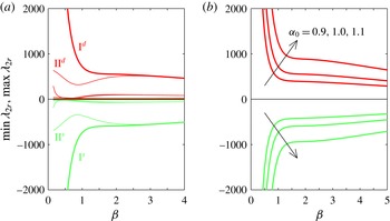
Variation of the leading growth rate for optimally destabilising flow modification (superscript
 $d$
, dark lines, red online) and optimally stabilising flow modification (superscript
 $s$
, light lines, green online), as predicted by sensitivity analysis. (a) Optimisation for the leading eigenmode of wavenumbers
 $({\it\alpha}_{0},{\it\beta}_{0})=(1,0)$
. Suboptimals are also shown as thin lines. (b) Optimal growth rate variation for
 ${\it\alpha}_{0}=0.9,1.0,1.1$
and
 ${\it\beta}_{0}=0$
.

3. Results: the plane channel
We investigate the parallel flow in a plane channel between solid walls located at
 $y=\pm 1$
. The base flow has a Poiseuille parabolic profile
 $U_{0}(y)=1-y^{2}$
and first becomes linearly unstable at
 $\mathit{Re}=5772$
. We solve the eigenvalue problem (2.3) in primitive variables
 $(\boldsymbol{u},p)^{\text{T}}$
with a 1D spectral method using
 $N=100$
Chebyshev polynomials (Trefethen Reference Trefethen2000) on
 $y\in [-1;1]$
and homogeneous Dirichlet boundary conditions on velocity components. The method was validated against spectral results in Orr–Sommerfeld variables (Schmid & Henningson Reference Schmid and Henningson2001), yielding
 $10^{-8}$
accuracy with
 $N=35$
polynomials. We focus on the Reynolds number
 $\mathit{Re}=6000$
, where the largest growth rate is obtained for wavenumbers
 $({\it\alpha}_{0},{\it\beta}_{0})=({\it\alpha}_{0,max},{\it\beta}_{0,max})=(1.016,0)$
, and the leading eigenvalue
 ${\it\lambda}_{0}=3.694\times 10^{-4}-0.2659\text{i}$
corresponds to a 2D Tollmien–Schlichting wave.
3.1. Optimal flow modifications
We compute the most destabilising and most stabilising spanwise-periodic flow modifications according to (2.16). Figure 2(a) shows the largest positive and negative second-order eigenvalue variations at
 $({\it\alpha}_{0},{\it\beta}_{0})=(1,0)$
as a function of the control spanwise wavenumber
 ${\it\beta}$
. The curves labelled I
 $^{d}$
and I
 $^{s}$
provide bounds for the largest possible destabilisation and stabilisation. As shown in figure 2(b), the upper and lower bounds increase with
 ${\it\alpha}_{0}$
, indicating that optimal flow modifications have a stronger effect on leading eigenmodes of smaller streamwise wavelengths. It should be noted that
 $\min {\it\lambda}_{2r}$
and
 $\max {\it\lambda}_{2r}$
are of the same order of magnitude in absolute value.
Figure 2(a) also shows growth rate variations for suboptimal flow modifications (thin lines). The first suboptimal modifications (branches II
 $^{d}$
, II
 $^{s}$
) become as effective as the optimal ones when
 ${\it\beta}\geqslant 2.5$
.
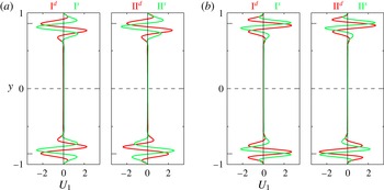
For all wavenumbers
 ${\it\beta}$
, the optimal stabilising and destabilising modifications for
 $({\it\alpha}_{0},{\it\beta}_{0})=(1,0)$
, shown in figure 3, are symmetric in
 $y$
, and are localised close to the critical layer, where the base flow velocity is equal to the phase speed of the Tollmien–Schlichting wave (
 $y=\pm 0.86$
). The first suboptimals have similar structures but are antisymmetric.
Optimal (branch I) and first suboptimal (branch II) destabilising (dark, red online) and stabilising (light, green online) base flow modification for the most unstable mode
 $({\it\alpha}_{0},{\it\beta}_{0})=({\it\alpha}_{0,max},{\it\beta}_{0,max})=(1,0)$
, at control wavenumbers
 ${\it\beta}=0.4$
(a) and
 ${\it\beta}=3$
(b). The long ticks on the left show the positions of the critical layers at
 $y=\pm 0.86$
.

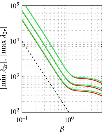
For small values of
 ${\it\beta}$
, the upper and lower bounds diverge like
 ${\it\beta}^{-2}$
, as shown in figure 4. This points to a strong authority of the flow modification as its spanwise wavelength tends to infinity. This diverging effect at small
 ${\it\beta}$
was also observed by Cossu (Reference Cossu2014) and Del Guercio et al. (Reference Del Guercio, Cossu and Pujals2014) for a specific choice of base flow modification (streaks created by optimal streamwise vortices in a 2D wake, and uniform modification in a 1D Ginzburg–Landau equation respectively). Based on an expansion on the eigenmodes of the unperturbed problem (Hinch Reference Hinch1991), this phenomenon was explained by Tammisola et al. (Reference Tammisola, Giannetti, Citro and Juniper2014) as a modal resonance between unperturbed eigenmodes having close eigenvalues, namely the eigenmode of interest (2D mode
 ${\it\beta}_{0}=0$
in our case), and eigenmodes whose spanwise wavenumbers differ by
 $\pm {\it\beta}$
from that of the eigenmode of interest (i.e.
 ${\it\beta}_{0}=\pm {\it\beta}$
). We show in appendix D that the eigenvalue difference between the 2D eigenmode of interest and eigenmodes of small spanwise wavenumber
 ${\it\beta}_{0}=\pm {\it\beta}$
scales precisely like
 ${\it\beta}^{2}$
, consistent with the divergence behaviour
 ${\it\lambda}_{2}\sim {\it\beta}^{-2}$
we observe. It should be mentioned in this context (Tammisola et al.
Reference Tammisola, Giannetti, Citro and Juniper2014) that if
 ${\it\beta}$
is small enough that the eigenvalue difference between these modes is small and of order
 ${\rm\Delta}{\it\lambda}\sim {\it\epsilon}$
, then the modal resonance results in a non-small second-order eigenvalue variation
 ${\it\lambda}_{2}=O({\it\epsilon}/{\rm\Delta}{\it\lambda})=O(1)$
and the perturbation approach (2.4) is not valid any longer. Experimentally, the spanwise extension of the system sets a minimal value for
 ${\it\beta}$
.
Optimal eigenvalue variations diverge like
 ${\it\beta}^{-2}$
as the control wavenumber decreases (same data as figure 2 in logarithmic scale,
 ${\it\alpha}_{0}=0.9,1.0,1.1$
,
 ${\it\beta}_{0}=0$
).

Effect of optimal 2D flow modification (spanwise-periodic, control wavenumber
 ${\it\beta}=1$
) on the growth rate of the leading eigenmode
 $({\it\alpha}_{0},{\it\beta}_{0})=(1,0)$
. The lines show the 1D sensitivity prediction and the symbols show the full 2D stability calculations.

3.2. Validation
In order to validate the sensitivity analysis, full 2D calculations were performed on base flows with optimally stabilising spanwise-periodic modifications. The numerical method is the following. Equations (2.3) are discretised on the computational domain
 $y\in [-1;1]$
,
 $z\in [0;5\times 2{\rm\pi}/{\it\beta}]$
with the finite element solver FreeFem++ (Hecht Reference Hecht2012) using P2 elements for velocity components and P1 elements for pressure; homogeneous Dirichlet boundary conditions
 $\boldsymbol{u}=\mathbf{0}$
are imposed at
 $y=\pm 1$
, while periodic boundary conditions are imposed on lateral boundaries (
 $z=0$
,
 $z=5\times 2{\rm\pi}/{\it\beta}$
); finally the library SLEPc (Hernandez, Roman & Vidal Reference Hernandez, Roman and Vidal2005) is used to compute generalised eigenpairs of the eigenvalue problem with base flow
 $U_{0}(y)+{\it\epsilon}U_{1}(y)\cos ({\it\beta}z)$
, and
 $U_{1}$
of unit 1D norm.
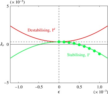
Figure 5 shows how the growth rate of the leading eigenmode varies with the control amplitude, when the most stabilising/destabilising flow modifications are optimised for control wavenumber
 ${\it\beta}=1$
and eigenmode
 $({\it\alpha}_{0},{\it\beta}_{0})=(1,0)$
. In the stabilising case, the agreement between 1D sensitivity predictions (solid line) and full 2D calculations (symbols) is excellent. As expected,
 ${\it\lambda}_{r}$
varies quadratically with
 ${\it\epsilon}$
.
3.3. Robustness
A question of interest is whether the most stabilising flow modification obtained for
 ${\it\alpha}_{0}={\it\alpha}_{0,max}$
and
 ${\it\beta}_{0}={\it\beta}_{0,max}$
is stabilising at other wavenumbers too. In other words, is the optimisation robust? We investigate this question by choosing flow modifications optimised for the leading mode
 $({\it\alpha}_{0},{\it\beta}_{0})=(1,0)$
and computing their effect on other modes
 $({\it\alpha}_{0},{\it\beta}_{0})\neq ({\it\alpha}_{0,max},{\it\beta}_{0,max})$
.
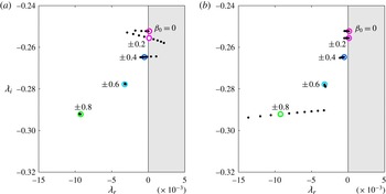
Figure 6 shows eigenspectra when the base flow is modified with control wavenumbers
 ${\it\beta}=0.4$
and
 ${\it\beta}=1.6$
. The 2D mode
 ${\it\beta}_{0}=0$
is fully restabilised as predicted by sensitivity analysis. Three-dimensional modes are stabilised or destabilised depending on
 ${\it\beta}$
and
 ${\it\beta}_{0}$
. A splitting of modes
 ${\it\beta}_{0}=\pm {\it\beta}$
and
 ${\it\beta}_{0}=\pm {\it\beta}/2$
is systematically observed as a result of the flow modification and of a subharmonic resonance, and is consistent with Floquet analyses in other spatially periodic flows (Herbert Reference Herbert1988; Hwang et al.
Reference Hwang, Kim and Choi2013). Therefore, the use of small flow modification wavenumbers (figure 6
a) yields a large stabilising effect on the leading 2D mode, as discussed in § 3.1, but this also destabilises some slightly damped 3D eigenmodes. The choice of larger values of
 ${\it\beta}$
(figure 6
b) circumvents this issue since the 3D modes that undergo splitting are more stable, and so remain at the amplitude
 ${\it\epsilon}$
needed to fully restabilise the 2D mode and thus the whole flow.
Effect of the most stabilising spanwise-periodic flow modification
 ${\it\epsilon}U_{1}(y)\cos ({\it\beta}z)$
on leading 2D and 3D eigenvalues at
 ${\it\alpha}_{0}=1$
, with flow modification wavenumber (a)
 ${\it\beta}=0.4$
and (b)
 ${\it\beta}=1.6$
, and
 $U_{1}$
optimised for the most unstable eigenmode
 $({\it\alpha}_{0},{\it\beta}_{0})=(1,0)$
. The 3D eigenpair with
 ${\it\beta}_{0}=\pm {\it\beta}/2$
undergoes a splitting, and one of the two modes becomes unstable. This issue is avoided by choosing larger
 ${\it\beta}$
values, since the 3D eigenmodes affected by splitting are then very stable. In (a),
 ${\it\epsilon}=(0.18,0.35,0.53,0.71)\times 10^{-3}$
, and in (b),
 ${\it\epsilon}=(0.18,\ldots ,0.71,0.88,1.06)\times 10^{-3}$
.

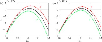
Next, we look at robustness in
 ${\it\alpha}_{0}$
. Figure 7 shows that whatever the choice of spanwise wavenumber
 ${\it\beta}$
, flow modifications optimised to stabilise (destabilise) the leading mode at
 ${\it\alpha}_{0,max}$
have a stabilising (destabilising) effect at all other values of
 ${\it\alpha}_{0}$
too.
Effect of optimal spanwise-periodic flow modification
 ${\it\epsilon}U_{1}(y)\!\,\cos ({\it\beta}z)$
on the leading growth rate with
 $U_{1}$
optimised for
 $({\it\alpha}_{0},{\it\beta}_{0})=({\it\alpha}_{0,max},{\it\beta}_{0,max})=(1,0)$
, at control wavenumber
 ${\it\beta}=1$
(a) and
 ${\it\beta}=3$
(b). Branch I
 $^{d}$
is the most destabilising one and branch I
 $^{s}$
is the most stabilising one;
 ${\it\epsilon}=0.001$
.

In this section we computed the optimal spanwise-periodic flow modifications yielding the largest second-order variation in growth rate, and showed that is was possible to fully restabilise the plane channel flow with small-amplitude modifications. In the next section, we turn to a more strongly unstable flow and investigate to what extent this strategy remains effective and robust.
4. Results: the parallel mixing layer
We now focus on the hyperbolic-tangent mixing layer
 $U_{0}(y)=1+R\!\,\tanh (y)$
(Michalke Reference Michalke1964) with
 $R=1$
, at
 $\mathit{Re}=100$
. Unlike the plane channel flow of § 3, which is unstable only in the neighbourhood of
 ${\it\alpha}_{0,max}=1$
with viscous eigenmodes characterised by weak growth rates, the mixing layer is unstable in the whole band of wavenumbers
 $0\leqslant {\it\alpha}_{0}\leqslant 1$
, and its inviscid eigenmodes exhibit much stronger growth rates. We use the same 1D spectral method as in § 3 on the domain
 $y\in [-5;5]$
with homogeneous Dirichlet boundary conditions on velocity components. The largest growth rate is obtained for the streamwise wavenumber
 ${\it\alpha}_{0}={\it\alpha}_{0,max}=0.45$
, where the leading eigenvalue is
 ${\it\lambda}_{0}=0.1676-0.4500\text{i}$
, in agreement with existing results (Betchov & Szewczyk Reference Betchov and Szewczyk1963; Michalke Reference Michalke1964; Villermaux Reference Villermaux1998).
4.1. Optimal flow modifications
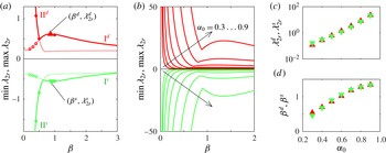
We compute the most destabilising and most stabilising spanwise-periodic flow modifications according to (2.16). Figure 8(a) shows the largest positive and negative second-order eigenvalue variations at
 ${\it\alpha}_{0}=0.5$
as a function of the control spanwise wavenumber. Again, these curves provide bounds for the largest possible destabilisation and stabilisation. Each of these two curves has a local extremum,
 ${\it\lambda}_{2r}^{d}$
and
 ${\it\lambda}_{2r}^{s}$
respectively, close to
 ${\it\beta}^{d}={\it\beta}^{s}=0.8$
. As shown in figure 8(b), for a fixed choice of
 ${\it\beta}$
the upper and lower bounds strongly increase with
 ${\it\alpha}_{0}$
, indicating that optimal flow modifications have a stronger effect on the leading eigenmode at smaller streamwise wavelengths. Figure 8(c) shows that the local extrema
 ${\it\lambda}_{2r}^{d}$
and
 ${\it\lambda}_{2r}^{s}$
increase exponentially, while the corresponding values of
 ${\it\beta}$
become slightly larger but remain of order
 ${\sim}$
1. For smaller values of
 ${\it\beta}$
, the upper and lower bounds diverge like
 ${\it\beta}^{-2}$
, like in the plane channel flow.
Upper and lower bounds on
 ${\it\lambda}_{2}$
, i.e. maximal destabilising (dark, red online) and stabilising (light, green online) effect on the leading growth rate, as predicted by sensitivity analysis. (a) For
 ${\it\alpha}_{0}=0.5$
, crossing of branches I and II, optimal at large and small
 ${\it\beta}$
respectively. The circles are calculations for the full stability problem. (b) Upper and lower bounds for
 ${\it\alpha}_{0}=0.3\ldots 0.9$
. (c,d) Variation with
 ${\it\alpha}_{0}$
of the local maxima and minima shown as triangles in (a), and corresponding spanwise wavenumbers.

The upper and lower bounds in figure 8(a) are actually made of two branches which intersect and correspond to different families of flow modifications
 $U_{1}$
. We call branch I the optimal family at large
 ${\it\beta}$
(corresponding to the local extrema at
 ${\it\beta}^{d}$
,
 ${\it\beta}^{s}$
) and branch II the optimal family at small
 ${\it\beta}$
(diverging as
 ${\it\beta}\rightarrow 0$
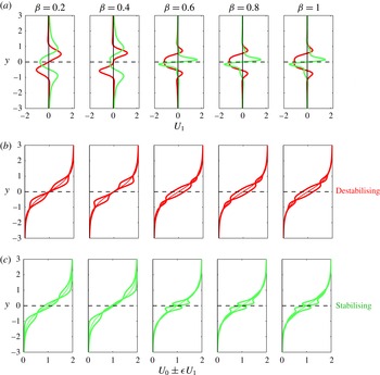
). Optimal modifications are shown in figure 9 for
 ${\it\alpha}_{0}={\it\alpha}_{0,max}=0.45$
. At small spanwise wavelength
 ${\it\beta}<0.5$
, the most destabilising
 $U_{1}$
is antisymmetric and the most stabilising
 $U_{1}$
is symmetric; at larger spanwise wavelength
 ${\it\beta}>0.5$
, symmetry properties are exchanged as branches I and II cross.
(a) Most destabilising (dark, red online) and stabilising (light, green online)
 $U_{1}$
for
 ${\it\alpha}_{0}={\it\alpha}_{0,max}=0.45$
. (b) Total modified flow
 $U_{0}(y)+{\it\epsilon}U_{1}(y)\cos ({\it\beta}z)$
at
 $z=0$
and
 $z={\rm\pi}/{\it\beta}$
for
 ${\it\epsilon}=0.2$
.

4.2. Validation
Similarly to § 3.2, we compare the effect of optimal spanwise-periodic flow modifications of unit 1D norm predicted by sensitivity analysis and obtained from full 2D calculations with the same numerical method as in §§ 3.2 and 3.3 on
 $y\in [-5;5]$
,
 $z\in [0;2\times 2{\rm\pi}/{\it\beta}]$
.
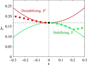
The variation of the leading growth rate
 $({\it\alpha}_{0},{\it\beta}_{0})=(0.45,0)$
for control wavenumber
 ${\it\beta}=0.8$
(branch I) is illustrated in figure 10. The agreement is good at small amplitudes
 $|{\it\epsilon}|\lesssim 0.2$
. At larger amplitudes, the actual growth rate departs from the expected quadratic dependence, due to nonlinear effects and to other modes becoming unstable. We have not investigated the splitting described in § 3.3 systematically.
Effect of optimal 2D (spanwise-periodic) flow modifications at
 ${\it\beta}=0.8$
on the leading growth rate at
 ${\it\alpha}_{0}={\it\alpha}_{0,max}=0.45$
. The lines show the sensitivity prediction and the symbols show the full stability calculations.

4.3. Robustness
Since the mixing layer is unstable over a wide range of streamwise wavenumbers, it is important to assess the robustness of the flow modifications designed for the most unstable mode
 ${\it\alpha}_{0}={\it\alpha}_{0,max}$
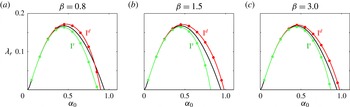
. We investigate this point by computing the variation in the leading growth rate predicted by (2.13) when the flow is modified with
 ${\it\epsilon}U_{1}(y)\cos ({\it\beta}z)$
, where
 ${\it\epsilon}=0.1$
and
 $U_{1}$
is chosen in branch I for
 ${\it\alpha}_{0}={\it\alpha}_{0,max}=0.45$
. Figure 11 shows that whatever the choice of spanwise wavenumber
 ${\it\beta}$
, flow modifications optimised to stabilise (destabilise) the leading mode at
 ${\it\alpha}_{0,max}$
have a stabilising (destabilising) effect at almost all other values of
 ${\it\alpha}_{0}$
too. This effect is negligible at small
 ${\it\alpha}_{0}$
, and larger at larger
 ${\it\alpha}_{0}$
. This is due to the dispersion relation at small
 ${\it\alpha}_{0}$
being independent of the details of the velocity profile: in particular, according to the Kelvin–Helmholtz dispersion relation
 ${\it\lambda}_{r}={\it\alpha}_{0}{\rm\Delta}U/2$
pertaining to the vorticity sheet model, the growth rate is only determined by the velocity difference
 ${\rm\Delta}U$
between the two streams. In contrast, the maximal growth rate and the cutoff wavenumber are influenced by other characteristics of the velocity profile (e.g. thickness and shear). Here, since
 $U_{1}(y)$
vanishes far from
 $y=0$
, the velocity difference
 ${\rm\Delta}U=2R$
remains constant, and so does the growth rate at small
 ${\it\alpha}_{0}$
.
Effect of optimal spanwise-periodic flow modification
 ${\it\epsilon}U_{1}(y)\cos ({\it\beta}z)$
on the leading growth rate with
 $U_{1}$
optimised for
 ${\it\alpha}_{0}={\it\alpha}_{0,max}=0.45$
and
 ${\it\beta}=0.8$
(a),
 ${\it\beta}=1.5$
(b),
 ${\it\beta}=3.0$
(c). Branch I
 $^{d}$
is the most destabilising one and branch I
 $^{s}$
is the most stabilising one;
 ${\it\epsilon}=0.1$
.

In this section we showed that strongly unstable eigenmodes in the mixing layer were made more stable by adding optimal 2D spanwise-periodic modifications to the base flow. Modifications designed for the most unstable streamwise wavenumber
 ${\it\alpha}_{0,max}$
have a stabilising effect on other unstable wavenumbers
 ${\it\alpha}_{0}$
. A wide range of modification wavenumbers
 ${\it\beta}$
were found to be effective. In the next section, we investigate how the impact of 2D spanwise-periodic modifications can be increased by taking advantage of non-normal transient growth, and achieving large modifications from initially small perturbations.
5. Leveraging transient growth to increase stabilisation
Non-normal mechanisms can lead to substantial transient growth in many flows (Butler & Farrell Reference Butler and Farrell1992; Trefethen et al. Reference Trefethen, Trefethen, Reddy and Driscoll1993; Schmid & Henningson Reference Schmid and Henningson2001). This phenomenon is thought to make possible subcritical transition to turbulence in linearly stable flows, like the flow in a circular pipe, since small-amplitude perturbations can undergo large (linear) amplification and eventually trigger (nonlinear) destabilisation. This potential for large amplification has also been exploited as a control strategy: it has been observed that streamwise vortices amplified into streamwise streaks through the lift-up mechanism are able to stabilise boundary layers (Cossu & Brandt Reference Cossu and Brandt2002; Fransson et al. Reference Fransson, Brandt, Talamelli and Cossu2005) and wakes (Del Guercio et al. Reference Del Guercio, Cossu and Pujals2014). It remains unclear, however, whether optimally amplified perturbations always have a stabilising effect, and whether there exist other perturbations that undergo a smaller amplification but eventually yield a larger stabilisation.
In this section we revisit this control strategy in terms of optimal flow modification. We consider the stabilising effect of spanwise-periodic perturbations undergoing transient amplification. This is similar in spirit to the study of Del Guercio et al. (Reference Del Guercio, Cossu and Pujals2014), but instead of computing a posteriori the stabilising effect of optimally amplified perturbations, we rather optimise simultaneously transient growth and stabilising effect at the time of maximal amplification, and we thus determine combined optimal perturbations. It should be noted that we do not aim at complete restabilisation but rather wish to determine what kind of structure yields the largest overall stabilising effect. The approach relies on an extension of the optimisation method presented earlier (§ 2.3).
While the stabilisation/destabilisation of streamwise streaks has been shown in the literature to depend on their amplitude, we consider the effect of arbitrary streamwise-invariant spanwise-periodic structures under the strong hypothesis of their linear transient evolution. This is an important limitation of the present analysis. As the streaks evolve nonlinearly, two effects may contribute to mitigate the present results: first, the amplitude may saturate (Cossu & Brandt Reference Cossu and Brandt2004), which would yield a quantitative difference; second and more importantly, nonlinear saturated streaks remain spanwise-periodic but they lose their pure sinusoidal character in
 $z$
, as higher harmonics are generated.
Another important limitation of the proposed approach is to consider, following Reddy et al. (Reference Reddy, Schmid, Baggett and Henningson1998) and Cossu & Brandt (Reference Cossu and Brandt2004), that a separation of time scales applies between the fast scale of the exponential instability of the nominal base flow and the rather slow scale of transient growth mechanisms.
Therefore, the proposed combined optimisation is not expected to yield quantitatively accurate results, but rather constitutes a means to investigate the mechanisms at hand in streaky flows. As explained later on, it will allow us to interpret streamwise streaks as particularly efficient structures that both benefit from transient growth and effectively stabilise the flow.
5.1. Combined optimisation
We first leave stabilisation aside and recall the concept of transient growth. Denoting energy amplification from 0 to
 $t$
as
 $G(t)=\Vert \boldsymbol{u}(t)\Vert ^{2}/\Vert \boldsymbol{u}(0)\Vert ^{2}$
, and
 $\boldsymbol{P}$
the linear operator that propagates perturbations in time according to (2.1) such that
 $\boldsymbol{u}(t)=\boldsymbol{P}(t)\boldsymbol{u}(0)$
, the optimal transient growth can be computed at every time
 $t$
as
 $$\begin{eqnarray}\displaystyle G_{opt}(t)=\max _{\Vert \boldsymbol{u}(0)\Vert =1}G(t) & = & \displaystyle \max _{\Vert \boldsymbol{u}(0)\Vert =1}\left(\boldsymbol{u}(t)\,|\,\boldsymbol{u}(t)\right)\end{eqnarray}$$
 $$\begin{eqnarray}\displaystyle & = & \displaystyle \max _{\Vert \boldsymbol{u}(0)\Vert =1}\left(\boldsymbol{P}(t)\boldsymbol{u}(0)\,|\,\boldsymbol{P}(t)\boldsymbol{u}(0)\right)\end{eqnarray}$$
 $$\begin{eqnarray}\displaystyle & = & \displaystyle {\it\lambda}_{max}\{\boldsymbol{P}^{\dagger }\boldsymbol{P}\},\end{eqnarray}$$
 $\boldsymbol{u}_{opt}(0)$
. The largest value of optimal transient growth over all times is reached for some time
 $T:G_{opt}(T)=\max _{t}G_{opt}(t)$
.
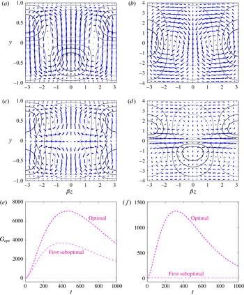
(a,b) Optimal and (c,d) first suboptimal perturbations for transient growth only. The arrows show the initial
 $(v,w)$
components (streamwise vortices) and the contours show the
 $u$
component after optimal amplification (streamwise streaks, low speed in dark, high speed in light). (e,f) Growth versus time for optimal and first suboptimal perturbations. (a,c,e) Plane channel flow,
 $\mathit{Re}=6000$
,
 $({\it\alpha},{\it\beta})=(0,2)$
; (b,d,f) mixing layer,
 $\mathit{Re}=100$
,
 $({\it\alpha},{\it\beta})=(0,0.35)$
.

Optimally amplified perturbations in the plane channel flow and in the mixing layer are shown in figure 12(a,b) for oblique perturbation wavenumbers
 $({\it\alpha},{\it\beta})=(0,2)$
and
 $({\it\alpha},{\it\beta})=(0,0.35)$
respectively. They lead to the maximal optimal growth over all wavenumbers
 $\max _{{\it\alpha},{\it\beta}}G_{opt}(T)=7047$
and
 $\max _{{\it\alpha},{\it\beta}}G_{opt}(T)=1328$
. In both flows, streamwise vortices at
 $t=0$
(arrows,
 $v$
and
 $w$
components) are amplified into streamwise streaks at
 $t=T$
(contours,
 $u$
component). The same computational method also yields a family of orthogonal suboptimal perturbations.
In the plane channel flow, the first suboptimal perturbation (shown in figure 12
c) leads to a maximal amplification
 $G_{subopt}=3694$
(figure 12
e). This is smaller than
 $G_{opt}(T)$
but of comparable order, while the amplification of following suboptimals is smaller by orders of magnitude, as already observed by Butler & Farrell (Reference Butler and Farrell1992). In the mixing layer, the first suboptimal perturbation (shown in figure 12
d) leads to a maximal amplification
 $G_{subopt}=16$
, two orders of magnitude smaller than
 $G_{opt}(T)$
(figure 12
f). In both flows, the typical time scale for transient growth/decay is of the order of
 $10^{2}$
.
If we now turn to combined optimisation, we look for perturbations that, after amplification, lead to maximal stabilisation. We optimise for the combined stabilising effect
 ${\it\lambda}_{2r}^{c}$
as
 $$\begin{eqnarray}\displaystyle \min _{\Vert \boldsymbol{u}(0)\Vert =1}{\it\lambda}_{2r}^{c} & = & \displaystyle \min _{\Vert \boldsymbol{u}(0)\Vert =1}\left(\left.u(t)\,\right|\,{\textstyle \frac{1}{2}}(\widetilde{\unicode[STIX]{x1D64E}}_{2r}+\widetilde{\unicode[STIX]{x1D64E}}_{2r}^{\text{T}})u(t)\right)\end{eqnarray}$$
 $$\begin{eqnarray}\displaystyle & = & \displaystyle \min _{\Vert \boldsymbol{u}(0)\Vert =1}\left(\left.\boldsymbol{P}_{u}(t)\boldsymbol{u}(0)\,\right|\,{\textstyle \frac{1}{2}}(\widetilde{\unicode[STIX]{x1D64E}}_{2r}+\widetilde{\unicode[STIX]{x1D64E}}_{2r}^{\text{T}})\boldsymbol{P}_{u}(t)\boldsymbol{u}(0)\right)\end{eqnarray}$$
 $$\begin{eqnarray}\displaystyle & = & \displaystyle {\it\lambda}_{min}\left\{{\textstyle \frac{1}{2}}\boldsymbol{P}_{u}^{\dagger }(\widetilde{\unicode[STIX]{x1D64E}}_{2r}+\widetilde{\unicode[STIX]{x1D64E}}_{2r}^{\text{T}})\boldsymbol{P}_{u}\right\}.\end{eqnarray}$$
 $U_{1}=u(t)$
as the flow modification in (2.16) and neglected
 $v$
and
 $w$
components, which will be justified a posteriori. Accordingly,
 $\boldsymbol{P}_{u}$
is a shorthand notation for the action of
 $\boldsymbol{P}$
followed by an extraction of the streamwise component. The combined optimal perturbation is denoted
 $\boldsymbol{u}_{opt}^{c}$
.
5.2. Results
Optimisation was carried out with transient growth at oblique wavenumbers
 $({\it\alpha},{\it\beta})=(0,{\it\beta})$
, and with destabilisation/stabilisation of the most unstable mode
 $({\it\alpha}_{0},{\it\beta}_{0})=({\it\alpha}_{0,max},0)$
. In this section we focus on the mixing layer flow at
 $\mathit{Re}=100$
, where the characteristic instability time scale
 $1/{\it\lambda}_{r}$
is of the order of
 $10^{0}$
, much smaller than the evolution time scale of the streaks. In the plane channel flow at
 $\mathit{Re}=6000$
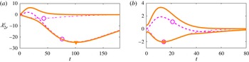
, the instability is weaker and the separation of time scales does not hold. The evolution of combined optimal effects is shown as thick lines in figure 13. At
 $t=0$
, the result of the optimisation is simply the optimal flow modification without transient growth, as already presented in § 4. At later times, the combined optimisation identifies perturbations that achieve the best trade-off between amplification from 0 to
 $t$
and destabilisation/stabilisation at
 $t$
.
Optimisation at
 ${\it\beta}=1$
yields a large stabilising effect over an extended time interval, thanks to the combination of amplification and flow modification. Indeed, combined optimal perturbations are very similar to transient growth-only optimal perturbations, whose effect (dashed line) is as large as the combined optimal effect.
At
 ${\it\beta}=2$
, however, transient growth-only optimal perturbations have a destabilising effect and therefore cannot be used to control the flow. Nevertheless, a stabilising combined effect can be obtained by choosing other perturbations, as indicated by the lower thick line. The stabilising combined optimal perturbations turn out to be similar to the first suboptimal perturbations for transient growth, which exploit the same lift-up mechanism but have the opposite symmetry in
 $y$
: two vortices amplified into two streaks on each side of the shear layer (figure 12
d), whereas optimal perturbations consist of one single vortex amplified into one streak centred in
 $y=0$
(figure 12
b).
Optimal combined transient growth and eigenvalue variation in the mixing layer at
 $\mathit{Re}=100$
. The thick lines show the optimal combined effects for stabilisation and destabilisation; the triangles indicate the maximal stabilising effect over all times. The dashed lines (respectively thin dash-dotted lines) show the optimal (respectively first suboptimal) perturbations for transient growth only; the circles show the corresponding eigenvalue variation at optimal amplification time. Transient growth at (a)
 $({\it\alpha}=0,{\it\beta}=1)$
and (b)
 $({\it\alpha}=0,{\it\beta}=2)$
; effect on the leading eigenvalue
 $({\it\alpha}_{0},{\it\beta}_{0})=(0.45,0)$
.

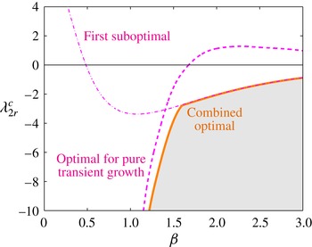
The largest stabilising effect
 ${\it\lambda}_{2r}^{c}$
(thick line) obtained from the combined optimisation of transient growth and eigenvalue variation versus the control wavenumber
 ${\it\beta}$
. Any other perturbation falls above the thick line, i.e. outside the grey region. The dashed line (respectively thin dash-dotted line) shows the stabilising effect of transient growth-only optimal (respectively first suboptimal) perturbations. Mixing layer,
 $\mathit{Re}=100$
,
 ${\it\alpha}_{0}={\it\alpha}_{0,max}=0.45$
.

In all cases, we observed that the combined optimal perturbations quickly became and remained unidirectional: the
 $v_{opt}^{c}$
and
 $w_{opt}^{c}$
components were much smaller than
 $u_{opt}^{c}$
well before the time of largest destabilisation/stabilisation, which justifies (5.2).
Figure 14 summarises the variation of the maximal combined stabilising effect with
 ${\it\beta}$
. The thick line shows the optimum over all times, and therefore provides a bound for the eigenvalue variation. At small wavenumbers
 ${\it\beta}\lesssim 1.5$
, the effect of optimally amplified streaks closely follows the optimal combined stabilising effect. Combined optimal perturbations are very similar to optimally amplified perturbations, whose effect (dashed line) is of the same order, and is reached after a comparable amplification time. In this range of wavenumbers, the optimal strategy to stabilise the flow at minimal cost is therefore precisely to introduce optimally amplified streaks. Other types of perturbations do not perform as well, either because they undergo a smaller amplification or because the flow modification that they induce has a smaller stabilising effect. At larger wavenumbers
 ${\it\beta}\gtrsim 1.5$
, optimally amplified perturbations are destabilising. Instead, the largest combined stabilisation is obtained with the first suboptimal perturbations for transient growth (dash-dotted line), which exhibit smaller cross-stream structures but undergo the same lift-up mechanism.
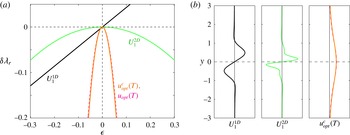
(a) Growth rate variation for combined optimal perturbations as a function of amplitude
 ${\it\epsilon}$
, compared with 1D and 2D optimal flow modifications for pure stabilisation. (b) Corresponding profiles of streamwise velocity: 1D optimal
 $U_{1}^{1D}$
, 2D optimal
 $U_{1}^{2D}$
and combined optimal after amplification
 $u_{opt}^{c}(T)$
. The optimal perturbation for pure transient growth
 $u_{opt}(T)$
is also shown as a dashed line superimposed onto the combined optimal, but the two curves are indistinguishable. Mixing layer,
 ${\it\beta}=0.8$
, eigenmode
 $({\it\alpha}_{0},{\it\beta}_{0})=(0.45,0)$
,
 $\mathit{Re}=100$
.

5.3. Discussion
In previous sections we have presented optimally stabilising flow modifications
 $U_{1}$
, optimal perturbations
 $u_{opt}$
for transient growth only, and combined optimal perturbations
 $u_{opt}^{c}$
for transient growth and stabilisation. We now compare the effect of these 2D (spanwise-periodic) modulations with the effect of 1D (spanwise-invariant) base flow modifications. Since the effect of spanwise-periodic modifications
 ${\it\epsilon}U_{1}(y)\cos ({\it\beta}z)$
is quadratic,
 $|{\it\lambda}-{\it\lambda}_{0}|\sim {\it\epsilon}^{2}$
, one can expect that it should be overcome at small amplitudes
 ${\it\epsilon}$
by the non-zero linear effect
 $|{\it\lambda}-{\it\lambda}_{0}|\sim {\it\epsilon}$
of spanwise-invariant modifications
 ${\it\epsilon}U_{1}^{1D}(y)$
. We use first-order sensitivity (Bottaro, Corbett & Luchini Reference Bottaro, Corbett and Luchini2003) to compute the eigenvalue sensitivity to 1D flow modification
 $S_{1}=\boldsymbol{e}_{x}\boldsymbol{\cdot }(-\boldsymbol{u}_{0}^{\dagger }\boldsymbol{\cdot }\boldsymbol{{\rm\nabla}}\boldsymbol{u}_{0}^{H}+\overline{\boldsymbol{u}}_{0}\boldsymbol{\cdot }\boldsymbol{{\rm\nabla}}\boldsymbol{u}_{0}^{\dagger })=\text{i}{\it\alpha}_{0}(2\overline{u}_{0}u_{0}^{\dagger }+\overline{v}_{0}v_{0}^{\dagger })+\overline{v}_{0}\partial _{y}u_{0}^{\dagger }$
. We then deduce the optimal 1D flow modification, equal to the real part of the sensitivity itself,
 $U_{1}^{1D}=S_{1r}$
, and the maximal growth rate variation,
 $\max {\it\lambda}_{1r}=\left(S_{1r}\,|\,U_{1}^{1D}\right)=\left(S_{1r}\,|\,S_{1r}\right)$
.
We compare in figure 15(a) the effects of optimal 1D and 2D flow modifications of unit norm per unit spanwise length, taking into account the total cost of modifying the flow over a given
 $z$
region. For intermediate wavenumber values (here
 ${\it\beta}=0.8$
) and for the amplitudes of interest, the optimal 1D flow modification
 $U_{1}^{1D}$
has a stronger stabilising effect than its 2D counterpart
 $U_{1}$
(also denoted
 $U_{1}^{2D}$
for clarity). Remarkably, combined optimal perturbations
 $u_{opt}^{c}$
have an even larger stabilising effect, as a result of transient growth. As mentioned earlier,
 $u_{opt}$
has an effect very similar to that of
 $u_{opt}^{c}$
for the wavenumber considered here.
Figure 15(b) shows the corresponding velocity profiles. The optimal 1D modification appears to be qualitatively similar to the optimally stabilising 2D modification:
 $U_{1}^{1D}$
has antisymmetric structures localised on each side of the shear layer but farther away than
 $U_{1}^{2D}$
(in a fashion actually similar to the optimally destabilising 2D modification at small wavenumber; see figure 9). It should be noted that for 1D spanwise-invariant flow modification it is enough to change the sign of
 $U_{1}^{1D}$
to turn a stabilising effect into a destabilising one and vice versa, in contrast to 2D spanwise-periodic flow modification, since stabilising and destabilising
 $U_{1}^{2D}$
have different structures (figures 3 and 9).
Combined optimal perturbations
 $u_{opt}^{c}$
have radically different velocity profiles, more widely distributed than
 $U_{1}$
and with the opposite symmetry. This is the result of initial perturbations being smoothed out by diffusion during transient amplification; one can therefore expect that these optimal structures would be easier to produce robustly in experiments. Again, it also indicates that combined optimal perturbations have an intrinsic stabilising effect that is suboptimal when considered alone, but they achieve a large combined stabilising effect when taking advantage of amplification.
6. Conclusion
We have determined analytically the second-order sensitivity of the leading eigenvalue in parallel flows with respect to small-amplitude spanwise-periodic velocity modifications of wavenumber
 ${\it\beta}$
. The explicit derivation of a second-order sensitivity operator allowed us to obtain the eigenvalue variation induced by any such flow modification without ever solving the modified eigenvalue problem or calculating the first-order eigenmode correction. Predictions from sensitivity analysis have been validated against numerical calculations of the full stability problem, and quadratic variations with modification amplitude were observed.
For any pair of eigenmode streamwise wavenumber
 ${\it\alpha}_{0}$
and base flow modification spanwise wavenumber
 ${\it\beta}$
, we have maximised the eigenvalue variation and determined the most destabilising and stabilising flow modifications. In the plane channel flow, the optimal modifications are localised close to the walls near critical layers, and show little variation with
 ${\it\beta}$
; in the mixing layer, they are centred around the location of maximum shear, and become more concentrated with increasing
 ${\it\beta}$
.
We observed that the optimal variations in growth rate increased like
 ${\it\lambda}_{2r}\sim {\it\beta}^{-2}$
for small control wavenumbers, and explained that this scaling was consistent with an interaction between unperturbed 2D and 3D eigenmodes. Spanwise-periodic flow modifications also appeared to have a larger effect on modes of larger streamwise wavenumber
 ${\it\alpha}_{0}$
. Modifications optimised for the most unstable mode have a robust effect on modes with other
 ${\it\alpha}_{0}$
. A splitting of 3D modes with
 ${\it\beta}_{0}=\pm {\it\beta}$
and
 ${\it\beta}_{0}=\pm {\it\beta}/2$
suggests the choice of large enough control wavenumbers so as not to destabilise weakly damped 3D modes.
In a second step aimed at increasing the stabilising effect and thus reducing the required control amplitude, we optimised simultaneously the linear transient growth of initial perturbations and the subsequent eigenvalue variation induced by the resulting flow modification, under the assumption of separation of time scales between transient growth and instability. In the mixing layer, this combined optimisation revealed that the perturbations undergoing the largest transient growth were also the combined optimals for small enough control wavenumbers,
 ${\it\beta}\lesssim 1.5$
, which justifies a posteriori the ‘vaccination’ strategy proposed by Cossu & Brandt (Reference Cossu and Brandt2002) to take advantage of the amplification of streamwise vortices into streamwise streaks through lift-up. As
 ${\it\beta}$
increases, optimally amplified perturbations gradually become destabilising, and the combined optimal turns out to correspond to the first suboptimal for pure transient growth.
The method readily applies to the quadratic sensitivity of the eigenmode frequency, if one wishes, for instance, to detune the vortex shedding frequency, and can easily be extended to other flow quantities.
Combined optimal perturbations could be created experimentally with a method similar to that of Fransson et al. (Reference Fransson, Brandt, Talamelli and Cossu2005), who used roughness elements in a boundary-layer flow to produce streamwise vortices amplified by transient growth into streamwise streaks. In the mixing layer these roughness elements could be placed on one or both sides of the splitting plate used to create the shear layer. One could also imagine using wall actuation to create the initial streamwise vortices.
We are presently working on generalising the second-order optimisation technique presented in this paper to non-parallel flows. In spatially developing flows, the method is conceptually similar but involves a number of complications. First, the large number of degrees of freedom prevents the explicit calculation of the inverse operator
 $({\it\lambda}_{0}\unicode[STIX]{x1D640}+\unicode[STIX]{x1D63C}_{0})^{-1}$
, but optimisation should still be possible since it only requires repeated evaluations of matrix–vector products. Second, the derivation of adjoint operators is technically more involved. In view of recent publications which describe the quadratic dependence of the growth rate on the amplitude of spanwise-periodic control in spatially developing flows such as wakes behind a circular cylinder (Kim & Choi Reference Kim and Choi2005; Del Guercio et al.
Reference Del Guercio, Cossu and Pujals2014) and behind a flat plate of finite thickness (Tammisola et al.
Reference Tammisola, Giannetti, Citro and Juniper2014), this generalisation appears to be a promising research direction.
Appendix A. Stability operators
We write explicitly the eigenvalue problem (2.3) for perturbations
 $\unicode[STIX]{x1D666}(y,z)\exp (\text{i}{\it\alpha}_{0}x+{\it\lambda}t)$
linearised around the base flow
 $U(y,z)\boldsymbol{e}_{x}$
:
 $$\begin{eqnarray}\displaystyle & {\it\lambda}u+\text{i}{\it\alpha}_{0}uU+v\partial _{y}U+w\partial _{z}U+\text{i}{\it\alpha}_{0}p-\mathit{Re}^{-1}\boldsymbol{{\rm\nabla}}_{{\it\alpha}_{0}}u=0, & \displaystyle\end{eqnarray}$$
 $$\begin{eqnarray}\displaystyle & {\it\lambda}v+\text{i}{\it\alpha}_{0}vU+\partial _{y}p-\mathit{Re}^{-1}\boldsymbol{{\rm\nabla}}_{{\it\alpha}_{0}}v=0, & \displaystyle\end{eqnarray}$$
 $$\begin{eqnarray}\displaystyle & {\it\lambda}w+\text{i}{\it\alpha}_{0}wU+\partial _{z}p-\mathit{Re}^{-1}\boldsymbol{{\rm\nabla}}_{{\it\alpha}_{0}}w=0, & \displaystyle\end{eqnarray}$$
 $$\begin{eqnarray}\displaystyle & \text{i}{\it\alpha}_{0}u+\partial _{y}v+\partial _{z}w=0, & \displaystyle\end{eqnarray}$$
 $\boldsymbol{{\rm\nabla}}_{{\it\alpha}_{0}}=-{\it\alpha}_{0}^{2}+\partial _{yy}+\partial _{zz}$
.
From the expansion (2.4), we find at leading order (
 ${\it\epsilon}^{0}$
) the eigenvalue problem (2.6)
 $({\it\lambda}_{0}\unicode[STIX]{x1D640}+\unicode[STIX]{x1D63C}_{0})\unicode[STIX]{x1D666}_{0}=\mathbf{0}$
, where
 $$\begin{eqnarray}\displaystyle & \unicode[STIX]{x1D640}=\left[\begin{array}{@{}cccc@{}}1 & 0 & 0 & 0\\ 0 & 1 & 0 & 0\\ 0 & 0 & 1 & 0\\ 0 & 0 & 0 & 0\end{array}\right], & \displaystyle\end{eqnarray}$$
 $$\begin{eqnarray}\displaystyle & \unicode[STIX]{x1D63C}_{0}=\left[\begin{array}{@{}cccc@{}}\text{i}{\it\alpha}_{0}U_{0}-\mathit{Re}^{-1}\boldsymbol{{\rm\nabla}}_{{\it\alpha}_{0}} & \partial _{y}U_{0} & 0 & \text{i}{\it\alpha}_{0}\\ 0 & \text{i}{\it\alpha}_{0}U_{0}-\mathit{Re}^{-1}\boldsymbol{{\rm\nabla}}_{{\it\alpha}_{0}} & 0 & \partial _{y}\\ 0 & 0 & \text{i}{\it\alpha}_{0}U_{0}-\mathit{Re}^{-1}\boldsymbol{{\rm\nabla}}_{{\it\alpha}_{0}} & \partial _{z}\\ \text{i}{\it\alpha}_{0} & \partial _{y} & \partial _{z} & 0\end{array}\right]. & \displaystyle\end{eqnarray}$$
At first order (
 ${\it\epsilon}^{1}$
) we find (2.7) for the first-order eigenmode correction
 $\unicode[STIX]{x1D666}_{1}$
, i.e.
 $({\it\lambda}_{0}\unicode[STIX]{x1D640}+\unicode[STIX]{x1D63C}_{0})\unicode[STIX]{x1D666}_{1}+({\it\lambda}_{1}\unicode[STIX]{x1D640}+\unicode[STIX]{x1D63C}_{1})\unicode[STIX]{x1D666}_{0}=\mathbf{0}$
, where
 $$\begin{eqnarray}\unicode[STIX]{x1D63C}_{1}=\left[\begin{array}{@{}cccc@{}}\text{i}{\it\alpha}_{0}U_{1}\cos ({\it\beta}z) & \partial _{y}U_{1}\cos ({\it\beta}z) & -{\it\beta}U_{1}\sin ({\it\beta}z) & 0\\ 0 & \text{i}{\it\alpha}_{0}U_{1}\cos ({\it\beta}z) & 0 & 0\\ 0 & 0 & \text{i}{\it\alpha}_{0}U_{1}\cos ({\it\beta}z) & 0\\ 0 & 0 & 0 & 0\end{array}\right].\end{eqnarray}$$
Appendix B. Sensitivity operators
The second-order eigenvalue variation (2.10) is manipulated in order to separate the base flow modification and the second-order sensitivity operator:
 ${\it\lambda}_{2}=((U_{1}\,|\,\unicode[STIX]{x1D64E}_{2}U_{1}))$
. To this aim, we introduce the adjoint operator
 $\unicode[STIX]{x1D63C}_{1}^{\dagger }$
such that
 $$\begin{eqnarray}{\it\lambda}_{2}=((\unicode[STIX]{x1D666}_{0}^{\dagger }\,|\,\unicode[STIX]{x1D63C}_{1}({\it\lambda}_{0}\unicode[STIX]{x1D640}+\unicode[STIX]{x1D63C}_{0})^{-1}\unicode[STIX]{x1D63C}_{1}\unicode[STIX]{x1D666}_{0}))=((\unicode[STIX]{x1D63C}_{1}^{\dagger }\unicode[STIX]{x1D666}_{0}^{\dagger }\,|\,({\it\lambda}_{0}\unicode[STIX]{x1D640}+\unicode[STIX]{x1D63C}_{0})^{-1}\unicode[STIX]{x1D63C}_{1}\unicode[STIX]{x1D666}_{0})),\end{eqnarray}$$
and we isolate the flow modification by rewriting
 $\unicode[STIX]{x1D63C}_{1}^{\dagger }\unicode[STIX]{x1D666}_{0}^{\dagger }=\unicode[STIX]{x1D648}U_{1}$
and
 $\unicode[STIX]{x1D63C}_{1}\unicode[STIX]{x1D666}_{0}=\unicode[STIX]{x1D647}U_{1}$
, where
 $$\begin{eqnarray}\unicode[STIX]{x1D648}=\left[\begin{array}{@{}c@{}}-\text{i}{\it\alpha}_{0}u_{0}^{\dagger }\cos ({\it\beta}z)\\ (u_{0}^{\dagger }\partial _{y}-\text{i}{\it\alpha}_{0}v_{0}^{\dagger })\cos ({\it\beta}z)\\ -{\it\beta}u_{0}^{\dagger }\sin ({\it\beta}z)\\ 0\end{array}\right],\quad \unicode[STIX]{x1D647}=\left[\begin{array}{@{}c@{}}(\text{i}{\it\alpha}_{0}u_{0}+v_{0}\partial _{y})\cos ({\it\beta}z)\\ \text{i}{\it\alpha}_{0}v_{0}\cos ({\it\beta}z)\\ 0\\ 0\end{array}\right].\end{eqnarray}$$
Finally, the second-order eigenvalue variation reads
 $$\begin{eqnarray}{\it\lambda}_{2}=((\unicode[STIX]{x1D648}U_{1}\,|\,({\it\lambda}_{0}\unicode[STIX]{x1D640}+\unicode[STIX]{x1D63C}_{0})^{-1}\unicode[STIX]{x1D647}U_{1}))=((U_{1}\,|\,\unicode[STIX]{x1D648}^{\dagger }({\it\lambda}_{0}\unicode[STIX]{x1D640}+\unicode[STIX]{x1D63C}_{0})^{-1}\unicode[STIX]{x1D647}U_{1})),\end{eqnarray}$$
where
 $$\begin{eqnarray}\unicode[STIX]{x1D648}^{\dagger }=[\text{i}{\it\alpha}_{0}\overline{u}_{0}^{\dagger }\cos ({\it\beta}z),\,(\text{i}{\it\alpha}_{0}\overline{v}_{0}^{\dagger }-\partial _{y}\overline{u}_{0}^{\dagger }-\overline{u}_{0}^{\dagger }\partial _{y})\cos ({\it\beta}z),\,-{\it\beta}\overline{u}_{0}^{\dagger }\sin ({\it\beta}z),\,0],\end{eqnarray}$$
and we identify the second-order sensitivity operator
 $\unicode[STIX]{x1D64E}_{2}=\unicode[STIX]{x1D648}^{\dagger }({\it\lambda}_{0}\unicode[STIX]{x1D640}+\unicode[STIX]{x1D63C}_{0})^{-1}\unicode[STIX]{x1D647}$
.
Appendix C. Transformation to spanwise-independent operators
We give details about the simplification of the second-order sensitivity operator, from the general expression
 $\unicode[STIX]{x1D64E}_{2}$
given in (2.12) to the
 $z$
-independent form
 $\widetilde{\unicode[STIX]{x1D64E}}_{2}$
given in (2.13), which is made possible by the explicit expressions of
 $\unicode[STIX]{x1D648}^{\dagger }$
and
 $\unicode[STIX]{x1D647}$
being available.
We denote
 $\unicode[STIX]{x1D656}=(a_{u},a_{v},a_{w},a_{p})^{\text{T}}$
a solution of
 $({\it\lambda}_{0}\unicode[STIX]{x1D640}+\unicode[STIX]{x1D63C}_{0})\unicode[STIX]{x1D656}=\unicode[STIX]{x1D647}U_{1}$
:
 $$\begin{eqnarray}\displaystyle & ({\it\lambda}_{0}+\text{i}{\it\alpha}_{0}U_{0}-\mathit{Re}^{-1}\boldsymbol{{\rm\nabla}}_{{\it\alpha}_{0}})a_{u}+\partial _{y}U_{0}a_{v}+\text{i}{\it\alpha}_{0}a_{p}=\cos ({\it\beta}z)(\text{i}{\it\alpha}_{0}u_{0}+v_{0}\partial _{y})U_{1}, & \displaystyle\end{eqnarray}$$
 $$\begin{eqnarray}\displaystyle & ({\it\lambda}_{0}+\text{i}{\it\alpha}_{0}U_{0}-\mathit{Re}^{-1}\boldsymbol{{\rm\nabla}}_{{\it\alpha}_{0}})a_{v}+\partial _{y}a_{p}=\cos ({\it\beta}z)\text{i}{\it\alpha}_{0}v_{0}U_{1}, & \displaystyle\end{eqnarray}$$
 $$\begin{eqnarray}\displaystyle & ({\it\lambda}_{0}+\text{i}{\it\alpha}_{0}U_{0}-\mathit{Re}^{-1}\boldsymbol{{\rm\nabla}}_{{\it\alpha}_{0}})a_{w}+\partial _{z}a_{p}=0, & \displaystyle\end{eqnarray}$$
 $$\begin{eqnarray}\displaystyle & \text{i}{\it\alpha}_{0}a_{u}+\partial _{y}a_{v}+\partial _{z}a_{w}=0. & \displaystyle\end{eqnarray}$$
 $$\begin{eqnarray}\unicode[STIX]{x1D656}=(\widetilde{a}_{u}\cos ({\it\beta}z),\widetilde{a}_{v}\cos ({\it\beta}z),\widetilde{a}_{w}\sin ({\it\beta}z),\widetilde{a}_{p}\cos ({\it\beta}z))^{\text{T}}.\end{eqnarray}$$
Therefore, the second-order eigenvalue variation reads
 $$\begin{eqnarray}\displaystyle {\it\lambda}_{2} & = & \displaystyle ((U_{1}\,|\,\unicode[STIX]{x1D64E}_{2}U_{1}))=((U_{1}\,|\,\unicode[STIX]{x1D648}^{\dagger }({\it\lambda}_{0}\unicode[STIX]{x1D640}+\unicode[STIX]{x1D63C}_{0})^{-1}\unicode[STIX]{x1D647}U_{1}))=((U_{1}\,|\,\unicode[STIX]{x1D648}^{\dagger }\unicode[STIX]{x1D656}))\end{eqnarray}$$
 $$\begin{eqnarray}\displaystyle & = & \displaystyle ((U_{1}\,|\,(\text{i}{\it\alpha}_{0}\overline{u}_{0}^{\dagger }\widetilde{a}_{u}+(\text{i}{\it\alpha}_{0}\overline{v}_{0}^{\dagger }-\partial _{y}\overline{u}_{0}^{\dagger }-\overline{u}_{0}^{\dagger }\partial _{y})\widetilde{a}_{v})\cos ^{2}({\it\beta}z)-{\it\beta}\overline{u}_{0}^{\dagger }\widetilde{a}_{w}\sin ^{2}({\it\beta}z)))\qquad\end{eqnarray}$$
 $$\begin{eqnarray}\displaystyle & = & \displaystyle {\textstyle \frac{1}{2}}\left(U_{1}\,|\,(\text{i}{\it\alpha}_{0}\overline{u}_{0}^{\dagger }\widetilde{a}_{u}+(\text{i}{\it\alpha}_{0}\overline{v}_{0}^{\dagger }-\partial _{y}\overline{u}_{0}^{\dagger }-\overline{u}_{0}^{\dagger }\partial _{y})\widetilde{a}_{v})-{\it\beta}\overline{u}_{0}^{\dagger }\widetilde{a}_{w}\right),\end{eqnarray}$$
 $\cos ^{2}({\it\beta}z)$
and
 $\sin ^{2}({\it\beta}z)$
over one spanwise wavelength being equal to
 ${\rm\pi}/{\it\beta}$
, yielding
 $1/2$
when normalised by the wavelength. Finally, the second-order sensitivity operator becomes independent of
 $z$
:
 $$\begin{eqnarray}{\it\lambda}_{2}=\left(\left.U_{1}\,\right|\,{\textstyle \frac{1}{2}}\widetilde{\unicode[STIX]{x1D648}}^{\dagger }({\it\lambda}_{0}\unicode[STIX]{x1D640}+\widetilde{\unicode[STIX]{x1D63C}}_{0})^{-1}\widetilde{\unicode[STIX]{x1D647}}U_{1}\right),\end{eqnarray}$$
where
 $$\begin{eqnarray}\widetilde{\unicode[STIX]{x1D648}}^{\dagger }=[\text{i}{\it\alpha}_{0}\overline{u}_{0}^{\dagger },\,\text{i}{\it\alpha}_{0}\overline{v}_{0}^{\dagger }-\partial _{y}\overline{u}_{0}^{\dagger }-\overline{u}_{0}^{\dagger }\partial _{y},\,-{\it\beta}\overline{u}_{0}^{\dagger },\,0],\quad \widetilde{\unicode[STIX]{x1D647}}=\left[\begin{array}{@{}c@{}}\text{i}{\it\alpha}_{0}u_{0}+v_{0}\partial _{y}\\ \text{i}{\it\alpha}_{0}v_{0}\\ 0\\ 0\end{array}\right],\end{eqnarray}$$
 $$\begin{eqnarray}\widetilde{\unicode[STIX]{x1D63C}}_{0}=\left[\begin{array}{@{}cccc@{}}\text{i}{\it\alpha}_{0}U_{0}-\mathit{Re}^{-1}\boldsymbol{{\rm\nabla}}_{{\it\alpha}_{0}{\it\beta}} & \partial _{y}U_{0} & 0 & \text{i}{\it\alpha}_{0}\\ 0 & \text{i}{\it\alpha}_{0}U_{0}-\mathit{Re}^{-1}\boldsymbol{{\rm\nabla}}_{{\it\alpha}_{0}{\it\beta}} & 0 & \partial _{y}\\ 0 & 0 & \text{i}{\it\alpha}_{0}U_{0}-\mathit{Re}^{-1}\boldsymbol{{\rm\nabla}}_{{\it\alpha}_{0}{\it\beta}} & -{\it\beta}\\ \text{i}{\it\alpha}_{0} & \partial _{y} & {\it\beta} & 0\end{array}\right]\end{eqnarray}$$
and
 $\boldsymbol{{\rm\nabla}}_{{\it\alpha}_{0}{\it\beta}}=-{\it\alpha}_{0}^{2}+\partial _{yy}-{\it\beta}^{2}$
.
Appendix D. Scaling in the small-
 ${\it\beta}$
limit

Consider the unperturbed base flow and the corresponding unstable 2D eigenmode
 $\unicode[STIX]{x1D666}_{0}$
solution of the eigenvalue problem
 $({\it\lambda}_{0}\unicode[STIX]{x1D640}+\unicode[STIX]{x1D63C}_{0})\unicode[STIX]{x1D666}_{0}=\mathbf{0}$
. There also exist 3D eigenmodes of spanwise wavenumber
 ${\it\beta}_{0}\neq 0$
, which are all less unstable. For small values of the spanwise wavenumber
 $|{\it\beta}_{0}|\ll 1$
, the eigenvalue varies like
 ${\it\lambda}({\it\beta}_{0})\simeq {\it\lambda}_{0}-C{\it\beta}_{0}^{2}$
,
 $C>0$
, as outlined in the following. We estimate the eigenvalue variation for a small change of spanwise wavenumber from
 ${\it\beta}_{0}=0$
to
 ${\it\beta}_{0}\ll 1$
by using the classical expression of first-order eigenvalue variation
 ${\it\delta}{\it\lambda}=-\left(\unicode[STIX]{x1D666}_{0}^{\dagger }\,|\,{\bf\delta}\unicode[STIX]{x1D63C}_{0}\unicode[STIX]{x1D666}_{0}\right)/\left(\unicode[STIX]{x1D666}_{0}^{\dagger }\,|\,\unicode[STIX]{x1D640}\unicode[STIX]{x1D666}_{0}\right)$
, where the variation of the linearised Navier–Stokes operator in this case is given by
 $$\begin{eqnarray}{\bf\delta}\unicode[STIX]{x1D63C}_{0}=\left[\begin{array}{@{}cccc@{}}\mathit{Re}^{-1}{\it\beta}_{0}^{2} & 0 & 0 & 0\\ 0 & \mathit{Re}^{-1}{\it\beta}_{0}^{2} & 0 & 0\\ 0 & 0 & \mathit{Re}^{-1}~{\it\beta}_{0}^{2} & \text{i}{\it\beta}_{0}\\ 0 & 0 & \text{i}{\it\beta}_{0} & 0\end{array}\right],\end{eqnarray}$$
and therefore
 ${\it\delta}{\it\lambda}=\mathit{Re}^{-1}{\it\beta}_{0}^{2}$
.
When the base flow is perturbed with a spanwise-periodic modification of long wavelength (small
 ${\it\beta}$
), there is interaction between the unperturbed 2D eigenmode of interest (
 ${\it\beta}_{0}=0$
) and the unperturbed 3D eigenmodes of spanwise wavenumber
 $\pm {\it\beta}$
, as described by Tammisola et al. (Reference Tammisola, Giannetti, Citro and Juniper2014); the resonance effect these authors proposed to explain large second-order sensitivity at small
 ${\it\beta}$
therefore leads in the present case to the second-order eigenvalue variation
 $|{\it\lambda}_{2}|\sim |{\it\delta}{\it\lambda}|^{-1}\sim {\it\beta}^{-2}$
, as observed in § 3.1.