1 Introduction
Non-Brownian suspensions of hard particles are commonly processed in many industries, among them the ceramics, oil, construction and food industries. They usually contain particles of various shapes and sizes in the range of a few micrometres. The suspended particles are large enough to experience no Brownian motion and relatively weak interparticle interactions besides steric repulsion, but are small enough for inertia to be neglected. These suspensions have very simple physical ingredients, yet they display a rather complex rheological behaviour. They exhibit normal stress differences (Zarraga, Hill & Leighton Reference Zarraga, Hill and Leighton2000; Singh & Nott Reference Singh and Nott2003; Boyer, Pouliquen & Guazzelli Reference Boyer, Pouliquen and Guazzelli2011b ; Couturier et al. Reference Couturier, Boyer, Pouliquen and Guazzelli2011; Dai et al. Reference Dai, Bertevas, Qi and Tanner2013; Dbouk, Lobry & Lemaire Reference Dbouk, Lobry and Lemaire2013), leading to unusual behaviours such as ‘rod dipping’ (Boyer et al. Reference Boyer, Pouliquen and Guazzelli2011b ). Also they commonly exhibit shear thinning (Gadala-Maria & Acrivos Reference Gadala-Maria and Acrivos1980; Zarraga et al. Reference Zarraga, Hill and Leighton2000; Singh & Nott Reference Singh and Nott2003; Blanc, Peters & Lemaire Reference Blanc, Peters and Lemaire2011b ; Dai et al. Reference Dai, Bertevas, Qi and Tanner2013) and, less commonly, shear thickening (Brown & Jaeger Reference Brown and Jaeger2009). For a recent review on these behaviours, see Denn & Morris (Reference Denn and Morris2014).
Systems composed of non-Brownian inertialess hard spheres, density-matched to a Newtonian suspending fluid, constitute the simplest idealized suspensions of this kind. They show apparently simple rate-independent rheological material functions (e.g. in simple shear, shear stress is proportional to the shear rate
 $\dot{\unicode[STIX]{x1D6FE}}$
, while normal stresses are proportional to
 $|\dot{\unicode[STIX]{x1D6FE}}|$
), albeit a non-Newtonian one (i.e. the viscosity is a fourth-rank tensor and not only a scalar). They have finite normal stress differences,
 $N_{2}$
being negative and dominant over
 $N_{1}$
, whose sign is still debated (Denn & Morris Reference Denn and Morris2014). Furthermore, there is a strong dependence of the rheology on the deformation history, as exemplified by the complex response observed in shear reversal experiments (Gadala-Maria & Acrivos Reference Gadala-Maria and Acrivos1980) or time-dependent deformations (Blanc, Lemaire & Peters Reference Blanc, Lemaire and Peters2014). Rate independence of the material functions follows from the fact that hard-sphere interactions have no characteristic stress scale or time scale, and so their amplitude is strictly proportional to the driving hydrodynamic forces. This means that the microstructure depends on strain history but not strain-rate history. Accordingly the microstructure in steady flow is independent of the strain rate. All stress components are then linear in strain rate (Denn & Morris Reference Denn and Morris2014). These simplifications can then be harnessed to develop phenomenological constitutive models (Hinch & Leal Reference Hinch and Leal1975).
Constitutive models of rheology have been successfully developed in the context of polymer solutions and melts (Larson Reference Larson2013). The simplest models (Johnson & Segalman Reference Johnson and Segalman1977; Giesekus Reference Giesekus1982) are based on a time-evolution equation of the (local) polymer stress tensor involving the polymer stress tensor itself as well as the strain-rate tensor. While these polymer stress models can be interpreted as consisting of two separate pieces, a proportionality relation between the polymer stress and the molecular conformation tensor, and a closed dynamical equation for the conformation tensor, the combination of these two elements leads to a single closed dynamical equation for the polymer stress tensor, and the fabric evolution is implicit. However, by construction, these models have a finite relaxation time and can only predict a continuous time evolution for the stress, a feature incompatible with the discontinuities observed in non-Brownian suspensions under discontinuous changes of imposed flow like shear reversal (Gadala-Maria & Acrivos Reference Gadala-Maria and Acrivos1980), due to the one-sidedness of contact forces. Instead, for non-Brownian suspensions, the constitutive models may require one to explicitly keep distinct the recipe linking the macroscopic stress to one or more microstructural state variables (which could then be explicitly alert to discontinuities in the imposed flow) and the closed (and continuous) dynamics for the microstructure. These two separate problems can be formulated top-down in a purely phenomenological manner, or derived bottom-up from the many-body microscopic dynamics, through either a coarse-graining procedure or a mechanistic approximation. In all cases, the resulting model is constrained by symmetry and frame-indifference considerations (Hand Reference Hand1962). The constitutive models for non-Brownian suspensions of Hinch & Leal (Reference Hinch and Leal1975), Phan-Thien (Reference Phan-Thien1995), Goddard (Reference Goddard2006) Stickel, Phillips & Powell (Reference Stickel, Phillips and Powell2006) follow this path, and pick for the microstructural variable a second-rank tensor
 $\unicode[STIX]{x1D64C}$
called the fabric tensor. A second-rank fabric tensor is the simplest object capturing anisotropies in the pair interaction network and is a natural candidate to inform a stress equation. Indeed, it has been recognized for some time that microstructural anisotropies play a central role in the stress response of dense suspensions (Batchelor & Green Reference Batchelor and Green1972; Gadala-Maria & Acrivos Reference Gadala-Maria and Acrivos1980; Wagner & Ackerson Reference Wagner and Ackerson1992; Blanc et al.
Reference Blanc, Lemaire, Meunier and Peters2013; Gurnon & Wagner Reference Gurnon and Wagner2015). Perhaps surprisingly, while they are apparently well-founded and follow conceptually from a history of successful polymer constitutive modelling, none of the fabric evolution equations for non-Brownian dense suspensions proposed so far has been thoroughly tested by comparison with detailed experimental or numerical data.
There are experimental reasons for this. While rheometric measurements for dense suspensions have been obtained under many different flow geometries and conditions (rate-controlled, stress-controlled or even particle-pressure-controlled (Boyer, Guazzelli & Pouliquen Reference Boyer, Guazzelli and Pouliquen2011a )), it is still challenging to obtain finely resolved microstructural data under rheometric flow. This is currently only accessible through confocal microscopy owing to the particle sizes involved (Cheng et al. Reference Cheng, McCoy, Israelachvili and Cohen2011), and, even then, the presence of even mild polydispersity confounds attempts to interrogate accurately the statistics of near-contacts. Note that the problem is spatial and not temporal resolution: in the rate-independent case, flow can be stopped at any time to inspect the structure and restarted without changing the subsequent dynamics.
Numerical simulations, on the other hand, can provide a high level of detail in the structure, and probe different flow conditions. Simple shear is by far the most common flow geometry studied, but others are possible, including planar elongational flow (Hwang & Hulsen Reference Hwang and Hulsen2006; Seto, Giusteri & Martiniello Reference Seto, Giusteri and Martiniello2017). Numerical data can be used not only to test the validity of constitutive models, but also to guide the development of new ones once relevant physical microscopic mechanisms are identified. The use of simulations is, however, subject to prior validation of the physical assumptions on which the numerical method is based, and this has proved a challenge for dense suspensions. The last few years have seen a breakthrough in this area with the recognition of the role of frictional contacts in the microstructure dynamics and stress response (Brown & Jaeger Reference Brown and Jaeger2012; Seto et al. Reference Seto, Mari, Morris and Denn2013; Mari et al. Reference Mari, Seto, Morris and Denn2014; Guy, Hermes & Poon Reference Guy, Hermes and Poon2015; Lin et al. Reference Lin, Guy, Hermes, Ness, Sun, Poon and Cohen2015), based on earlier experimental evidence (Castle, Farid & Woodcock Reference Castle, Farid and Woodcock1996; Lootens et al. Reference Lootens, Van Damme, Hémar and Hébraud2005; Blanc, Peters & Lemaire Reference Blanc, Peters and Lemaire2011a ). This has led to the development of numerical simulations which for the first time quantitatively match the experimental data for the rheology of dense suspensions (Gallier et al. Reference Gallier, Lemaire, Peters and Lobry2014; Lin et al. Reference Lin, Guy, Hermes, Ness, Sun, Poon and Cohen2015; Mari et al. Reference Mari, Seto, Morris and Denn2015). We recall that particle friction can preserve the rate independence of the rheology, provided that it does not introduce a rate or stress scale; many simple models of friction, like Coulomb friction used in this work, indeed lead to a rate-independent rheology (Gallier et al. Reference Gallier, Lemaire, Peters and Lobry2014; Mari et al. Reference Mari, Seto, Morris and Denn2014).
In this paper we leverage these new numerical simulation capabilities to interrogate the validity of the basic assumptions underlying fabric evolution models of the type so far used to build phenomenological constitutive equations. We present detailed numerical results for Stokesian dense suspensions of hard spheres interacting solely through near-field lubrication and Coulomb frictional contacts and subject to a shear reversal protocol. We emphasize the absence of additional short-ranged repulsions between particles: our system is not shear-thickening. Shear reversal is an informative probe of rheological mechanisms, and various experiments have measured the stress response under reversal for non-Brownian suspensions (Gadala-Maria & Acrivos Reference Gadala-Maria and Acrivos1980; Kolli, Pollauf & Gadala-Maria Reference Kolli, Pollauf and Gadala-Maria2002; Narumi et al. Reference Narumi, See, Honma, Hasegawa, Takahashi and Phan-Thien2002; Blanc et al. Reference Blanc, Peters and Lemaire2011b ). For hard-sphere suspensions, the shear reversal protocol retains the simplicity of shear flow while being one of the most stringent test cases for a microstructural description, as it probes the dependence on deformation history in perhaps its most extreme realization. Indeed, upon reversal, both hydrodynamic and contact force amplitudes are discontinuous. The hydrodynamic forces follow the discontinuous change of velocity field in the solvent, and a finite fraction of contacts are put under tension and thus instantaneously open, forcing a global load rebalance on the contact force network. Moreover, shear reversal is known to probe separately lubrication- and friction-dominated strain regimes (Lin et al. Reference Lin, Guy, Hermes, Ness, Sun, Poon and Cohen2015; Ness & Sun Reference Ness and Sun2016; Peters et al. Reference Peters, Ghigliotti, Gallier, Blanc, Lemaire and Lobry2016a ). We note that, since our system has shear rate as the only time scale, the microstructural evolution from a given starting state is fully determined by the sequence of strains thereafter, but not their rates. For instance, a smooth oscillatory shear is exactly equivalent, when expressed as a function of strain, to a series of instantaneous shear reversals between states of constant magnitude of the shear rate. More generally, shear reversal is a prototype for more complicated flows, such as biaxial shear (Lin et al. Reference Lin, Ness, Cates, Sun and Cohen2016) or the flow around a ball falling along the vorticity axis of a sheared suspension (Blanc et al. Reference Blanc, Lemaire and Peters2014; Peters, Majumdar & Jaeger Reference Peters, Majumdar and Jaeger2016b ), in which the structure of a sheared suspension is disrupted before a new structure is formed.
We find below that quantitative agreement between the fabric tensor dynamics and simulation data cannot be achieved in fabric evolution models; at least, not those that lend themselves to a simple physical interpretation. By interrogating the simulation data, we explore why fabric evolution in these systems is not well described by closed equations involving only the fabric tensor and the imposed flow. As will become clear, the fabric dynamics involves more details of the microstructure, some of which may be captured via higher spherical harmonics of the angular distribution of near-contacts.
In § 2, we explain our simulation protocol for acquiring shear reversal data. In § 3, we overview the fabric evolution approach, starting from the results of Hand (Reference Hand1962) for the frame-invariant dynamics of a second-rank tensor. In § 4, we introduce the family of fabric tensors whose dynamics we will consider, and start to develop models of increasing complexity within the Hand framework. In § 5, we show that the simplest families of possible fabric dynamics, restricted to linear or quadratic closures, fail to describe the dynamics of the system upon reversal. Using insights from two-dimensional simulations, in § 6 we show that models based on higher-order closures may fit the numerical data but are unlikely to be physically informed, and instead owe their fitting to the number of free parameters they contain. In § 7, we argue that the failure of fabric evolution models stems not from truncation at finite order in
 $\unicode[STIX]{x1D64C}$
but from the fact that the full distribution of near-contact directions
 $P(\boldsymbol{p})$
is dominated by a fourth-rank component, not coaxial with
 $\unicode[STIX]{x1D64C}$
, during part of the evolution following shear reversal. However, we speculate that the evolution of the microstructure dynamics might be satisfactorily closed by including both a second-rank fabric tensor
 $\unicode[STIX]{x1D64C}$
and a fourth-rank tensor that is not a function of the fabric and/or strain-rate tensors.
2 Simulation protocol
We simulate an assembly of non-inertial frictional spheres immersed in a Newtonian fluid under simple shear flow with an imposed velocity field
 $\boldsymbol{v}=(\dot{\unicode[STIX]{x1D6FE}}y,0,0)$
, using Lees–Edwards periodic boundary conditions (Lees & Edwards Reference Lees and Edwards1972). The system is bidisperse, with radii
 $a$
and
 $1.4a$
mixed at equal volume fractions. The particles interact solely through frictional contacts – with a friction coefficient
 $\unicode[STIX]{x1D707}=1$
, a value in agreement with measurements on non-colloidal quartz beads (Fernandez et al.
Reference Fernandez, Mani, Rinaldi, Kadau, Mosquet, Lombois-Burger, Cayer-Barrioz, Herrmann, Spencer and Isa2013), although other materials may show lower friction coefficients (Clavaud et al.
Reference Clavaud, Bérut, Metzger and Forterre2017; Comtet et al.
Reference Comtet, Chatté, Niguès, Bocquet, Siria and Colin2017) – and short-range hydrodynamic forces (lubrication) with a resistance divergence at contact truncated by a typical roughness length scale
 $\unicode[STIX]{x1D6FF}=10^{-3}a$
(Seto et al.
Reference Seto, Mari, Morris and Denn2013; Mari et al.
Reference Mari, Seto, Morris and Denn2014; Ness & Sun Reference Ness and Sun2016). Although actual hydrodynamic interactions have a many-body nature, considering only the short-ranged pairwise lubrication is a reasonable approximation at the large volume fractions we intend to investigate in this study (Ball & Melrose Reference Ball and Melrose1997). It has been shown that, for volume fractions
 $\unicode[STIX]{x1D719}>0.4$
, the major contribution to the total viscosity is from the contact forces (Gallier et al.
Reference Gallier, Lemaire, Peters and Lobry2014), and that long-ranged hydrodynamics has a near-negligible contribution to the hydrodynamic stress for volume fractions at least as low as
 $\unicode[STIX]{x1D719}=0.45$
(Mari et al.
Reference Mari, Seto, Morris and Denn2015). The contacts are modelled with the Cundall–Strack model (Cundall & Strack Reference Cundall and Strack1979) and thus are slightly deformable for purely numerical reasons. We use particles’ stiffness such that the overlaps are kept below a maximum of 2 % of a particle radius, which ensures a hard-sphere behaviour. We have tested that a doubling of the maximal overlap value does not affect the dynamics of the fabric tensor past a strain of roughly 1 % after reversal during which there is an elastic recoil from the contacts.
With these effectively hard-sphere interactions, the value of
 $\dot{\unicode[STIX]{x1D6FE}}$
only sets the speed at which the particles move on otherwise rate-independent trajectories. Similarly, the bulk stress (as well as both its hydrodynamic and contact components taken in isolation) is linear in
 $\dot{\unicode[STIX]{x1D6FE}}$
and
 $|\dot{\unicode[STIX]{x1D6FE}}|$
, that is, the rheological material functions are rate-independent. We performed the simulations at three volume fractions
 $\unicode[STIX]{x1D719}=0.4$
, 0.5 and 0.55 with
 $N=500$
particles. For reference, the jamming point for this system is at
 $\unicode[STIX]{x1D719}_{J}\approx 0.58$
(Mari et al.
Reference Mari, Seto, Morris and Denn2014). The simulation method, which is detailed in Mari et al. (Reference Mari, Seto, Morris and Denn2014), is briefly outlined in appendix A.
Starting from an overlap-free random initial configuration, the system is sheared in the
 $+x$
direction for 5 strain units (with imposed velocity gradient along
 $y$
), by which point the system has reached steady state. We then perform a flow reversal, and shear the system in the
 $-x$
direction for 3 strain units, during which structure is monitored continuously. In order to improve the statistics of our results, we repeat this procedure from 250 steady-state configurations. The data presented here are obtained from an average of these 250 flow reversal realizations.
3 Fabric-based microstructure description
3.1 Fabric tensor
In a non-Brownian hard-sphere suspension, particles interact solely through hydrodynamic and hard contact forces. While contact forces are short-range pairwise interactions, hydrodynamic forces result from the superposition of algebraically decaying solvent velocity fields created by the particles’ motion, and as such have a long-range and many-body nature. In a concentrated system, however, most of the hydrodynamic tractions on the particle surfaces come from lubrication flows within the narrow interparticle gaps (Frankel & Acrivos Reference Frankel and Acrivos1967). These lubrication forces are pairwise and short-ranged in nature. Therefore, in the dense regime, most of the stress comes from pairwise short-range interactions (Ball & Melrose Reference Ball and Melrose1997; Mari et al.
Reference Mari, Seto, Morris and Denn2015); indeed, the long-range hydrodynamics is omitted from our simulations, as described above. The pairwise nature of dominant forces will give a special importance for stress prediction to the pair correlation function
 $g(\boldsymbol{r})$
, defined as the conditional probability to find a particle whose centre is at
 $\boldsymbol{r}$
knowing that there is a particle at
 $\mathbf{0}$
, normalized by the average number density
 $\unicode[STIX]{x1D70C}$
. Moreover, because the dominant forces are also short-ranged and
 $g(\boldsymbol{r})$
is peaked at or very near contact (Morris & Katyal Reference Morris and Katyal2002; Nazockdast & Morris Reference Nazockdast and Morris2012, Reference Nazockdast and Morris2013; Mari et al.
Reference Mari, Seto, Morris and Denn2014), we can expect that only the near-contact part of
 $g(\boldsymbol{r})$
will play a substantial role. Hence we can consider the distribution of near-contact orientations
 $P(\boldsymbol{p})$
(with
 $\boldsymbol{p}\in S^{2}$
), which keeps only the orientational information of interactions that determine the stress state of the suspension.
Building a time-evolution dynamics for
 $P(\boldsymbol{p})$
(let alone
 $g(\boldsymbol{r})$
) is, however, very challenging for a non-Brownian suspension, and quite possibly over-reaching in the context of building a constitutive model. Indeed, the stress
 $\unicode[STIX]{x1D72E}$
is a symmetric second-rank tensor with six independent components, and in consequence contains far less information than the entire
 $P(\boldsymbol{p})$
. Therefore, rather than attempt to model the full
 $P(\boldsymbol{p})$
(or
 $g(\boldsymbol{r})$
(Nazockdast & Morris Reference Nazockdast and Morris2012, Reference Nazockdast and Morris2013)) directly, previous attempts model the symmetric and traceless fabric tensor
 $\unicode[STIX]{x1D64C}:=\langle \boldsymbol{p}\boldsymbol{p}\rangle -{\textstyle \frac{1}{3}}\unicode[STIX]{x1D644}$
. This is the deviatoric second moment of
 $P(\boldsymbol{p})$
, and the lowest-order moment carrying non-trivial structural information. It also corresponds to the second-order term in the Laplace spherical harmonic expansion of
 $P(\boldsymbol{p})$
in tensor form (Kanatani Reference Kanatani1984):
 $$\begin{eqnarray}\displaystyle P(\boldsymbol{p})\approx \frac{1}{4\unicode[STIX]{x03C0}}\left(1+\frac{15}{2}\unicode[STIX]{x1D64C}\boldsymbol{ : }\boldsymbol{p}\boldsymbol{p}\right). & & \displaystyle\end{eqnarray}$$
[For a symmetric distribution on the unit sphere like
 $P(\boldsymbol{p})$
, it is possible to define a tensorial expansion in powers of
 $\boldsymbol{p}$
as
 $P(\boldsymbol{p})=(1/(4\unicode[STIX]{x03C0}))\sum _{s=0}^{\infty }\unicode[STIX]{x1D60B}_{i_{1},\ldots ,i_{2s}}p_{i_{1}}\cdots p_{i_{2s}}$
such that the term of order
 $n=2s$
in the tensorial expansion is the projection of
 $P(\boldsymbol{p})$
on the
 $(2n+1)$
-dimensional space of Laplace spherical harmonics of order
 $n$
(Kanatani Reference Kanatani1984). Put differently, the order-
 $n$
term of the tensorial expansion is the sum of the terms of order
 $n$
in the Laplace spherical harmonics expansion. The tensors
 $\unicode[STIX]{x1D60B}_{i_{1},\ldots ,i_{n}}$
are deviatoric, hence contain
 $2n+1$
independent components, and are mutually independent, a consequence of the orthogonality of the Laplace spherical harmonics basis. The first-term tensor (zeroth rank) of the tensorial expansion is 1 (which enforces the normalization of
 $P(\boldsymbol{p})$
), the tensor of the second term is
 ${\textstyle \frac{15}{2}}\unicode[STIX]{x1D64C}$
.]
Retaining the fabric tensor
 $\unicode[STIX]{x1D64C}$
as a proxy for the full microstructure is indeed the standard choice made in previous attempts to build a constitutive model of suspensions (see Hinch & Leal Reference Hinch and Leal1975; Phan-Thien Reference Phan-Thien1995; Phan-Thien, Fan & Khoo Reference Phan-Thien, Fan and Khoo1999; Goddard Reference Goddard2006; Stickel et al.
Reference Stickel, Phillips and Powell2006). Note that there is also a long history of representing the microstructure via a second-rank tensor in polymeric systems (Larson Reference Larson2013) and in dry granular materials (Magnanimo & Luding Reference Magnanimo and Luding2011; Sun & Sundaresan Reference Sun and Sundaresan2011; Goddard Reference Goddard2014).
3.2 Dynamics: Hand equation
Once one decides to write the dynamics of the microstructure as a closed set of ordinary differential equations (ODEs) for the time evolution of the fabric tensor, symmetries and frame indifference (also known as material objectivity) constrain quite strongly the functional forms involved. In the absence of inertia, systems are invariant under time-dependent translations and rigid rotations, a property known as frame indifference. Using a representation theorem and enforcing frame indifference, one can write a general evolution equation for a symmetric
 $3\times 3$
tensor (Hand Reference Hand1962). Specifically, if
 $\text{d}\unicode[STIX]{x1D64C}/\text{d}t$
depends only on
 $\unicode[STIX]{x1D64C}$
itself and on the rate-of-strain tensor
 $\unicode[STIX]{x1D646}:=(\unicode[STIX]{x2202}_{j}v_{i})$
, where
 $\boldsymbol{v}$
is the local suspension velocity, we have
 $$\begin{eqnarray}\displaystyle \frac{\text{d}\unicode[STIX]{x1D64C}}{\text{d}t} & = & \displaystyle \unicode[STIX]{x1D652}\boldsymbol{\cdot }\unicode[STIX]{x1D64C}-\unicode[STIX]{x1D64C}\boldsymbol{\cdot }\unicode[STIX]{x1D652}+\tilde{\unicode[STIX]{x1D6FC}}_{0}\unicode[STIX]{x1D644}+\tilde{\unicode[STIX]{x1D6FC}}_{1}\unicode[STIX]{x1D64C}+\tilde{\unicode[STIX]{x1D6FC}}_{2}\unicode[STIX]{x1D640}+\tilde{\unicode[STIX]{x1D6FC}}_{3}\unicode[STIX]{x1D64C}^{2}+\tilde{\unicode[STIX]{x1D6FC}}_{4}\unicode[STIX]{x1D640}^{2}\nonumber\\ \displaystyle & & \displaystyle +\,\tilde{\unicode[STIX]{x1D6FC}}_{5}(\unicode[STIX]{x1D640}\boldsymbol{\cdot }\unicode[STIX]{x1D64C}+\unicode[STIX]{x1D64C}\boldsymbol{\cdot }\unicode[STIX]{x1D640})+\tilde{\unicode[STIX]{x1D6FC}}_{6}(\unicode[STIX]{x1D640}\boldsymbol{\cdot }\unicode[STIX]{x1D64C}^{2}+\unicode[STIX]{x1D64C}^{2}\boldsymbol{\cdot }\unicode[STIX]{x1D640})\nonumber\\ \displaystyle & & \displaystyle +\,\tilde{\unicode[STIX]{x1D6FC}}_{7}(\unicode[STIX]{x1D640}^{2}\boldsymbol{\cdot }\unicode[STIX]{x1D64C}+\unicode[STIX]{x1D64C}\boldsymbol{\cdot }\unicode[STIX]{x1D640}^{2})+\tilde{\unicode[STIX]{x1D6FC}}_{8}(\unicode[STIX]{x1D640}^{2}\boldsymbol{\cdot }\unicode[STIX]{x1D64C}^{2}+\unicode[STIX]{x1D64C}^{2}\boldsymbol{\cdot }\unicode[STIX]{x1D640}^{2}),\end{eqnarray}$$
where
 $\unicode[STIX]{x1D652}$
and
 $\unicode[STIX]{x1D640}$
are respectively the antisymmetric and symmetric parts of
 $\unicode[STIX]{x1D646}$
, and where the scalar coefficients
 $\tilde{\unicode[STIX]{x1D6FC}}_{i}$
are analytic functions of the invariants
 $I_{1}:=\text{Tr}[\unicode[STIX]{x1D64C}]$
,
 $I_{2}:=\text{Tr}[\unicode[STIX]{x1D64C}^{2}]$
,
 $I_{3}:=\text{Tr}[\unicode[STIX]{x1D64C}^{3}]$
,
 $I_{4}:=\text{Tr}[\unicode[STIX]{x1D640}]$
,
 $I_{5}:=\text{Tr}[\unicode[STIX]{x1D640}^{2}]$
,
 $I_{6}:=\text{Tr}[\unicode[STIX]{x1D640}^{3}]$
,
 $I_{7}:=\text{Tr}[\unicode[STIX]{x1D64C}\boldsymbol{\cdot }\unicode[STIX]{x1D640}]$
,
 $I_{8}:=\text{Tr}[\unicode[STIX]{x1D64C}^{2}\boldsymbol{\cdot }\unicode[STIX]{x1D640}]$
,
 $I_{9}:=\text{Tr}[\unicode[STIX]{x1D64C}\boldsymbol{\cdot }\unicode[STIX]{x1D640}^{2}]$
and
 $I_{10}:=\text{Tr}[\unicode[STIX]{x1D64C}^{2}\boldsymbol{\cdot }\unicode[STIX]{x1D640}^{2}]$
. Note that (3.2) follows only from frame indifference and the fact that
 $\unicode[STIX]{x1D64C}$
is a symmetric
 $3\times 3$
tensor. It does not rely on any specific physical property of the system nor on an expansion to some order in
 $\unicode[STIX]{x1D64C}$
or
 $\unicode[STIX]{x1D640}$
. As such, any closed ODE for
 $\text{d}\unicode[STIX]{x1D64C}/\text{d}t$
analytic in
 $\unicode[STIX]{x1D64C}$
and
 $\unicode[STIX]{x1D646}$
has to be of the form of (3.2).
In our case,
 $\unicode[STIX]{x1D64C}$
is traceless, which implies that
 $I_{1}=0$
and
 $\tilde{\unicode[STIX]{x1D6FC}}_{0}$
is prescribed by the value of the other coefficients
 $\tilde{\unicode[STIX]{x1D6FC}}_{i}$
. Incompressibility sets
 $\text{Tr}[\unicode[STIX]{x1D640}]=:I_{4}$
to zero too. We must, however, take special care when adopting Hand’s result for a non-Brownian hard-particle suspension. For a system with rate-independent particle trajectories, the fabric evolution must be proportional to the absolute value of the strain rate
 $|\dot{\unicode[STIX]{x1D6FE}}|=\sqrt{2\unicode[STIX]{x1D640}\boldsymbol{ :}\unicode[STIX]{x1D640}}$
. This is both necessary, because
 $\dot{\unicode[STIX]{x1D6FE}}$
is the only time scale, and permissible, because
 $\dot{\unicode[STIX]{x1D6FE}}=0$
corresponds to a singular case in which nothing evolves at all, so that analyticity must be defined on a domain in which
 $\dot{\unicode[STIX]{x1D6FE}}\neq 0$
. This is why the basic character of rate-independent rheology involves a linear dependence on
 $\dot{\unicode[STIX]{x1D6FE}}$
(for shear stress) or
 $|\dot{\unicode[STIX]{x1D6FE}}|$
(for normal stresses). The fabric evolution is then analytic in
 $\unicode[STIX]{x1D64C}$
and
 $\unicode[STIX]{x1D646}$
, except at
 $\unicode[STIX]{x1D646}=0$
(or equivalently
 $\dot{\unicode[STIX]{x1D6FE}}=0$
). Also, at least for the simple shear flows studied below, we can change variable from time to the accumulated strain
 $\unicode[STIX]{x1D6FE}$
. Hence, by introducing
 $\hat{\unicode[STIX]{x1D640}}=\unicode[STIX]{x1D640}/|\dot{\unicode[STIX]{x1D6FE}}|$
,
 $\hat{\unicode[STIX]{x1D652}}=\unicode[STIX]{x1D652}/|\dot{\unicode[STIX]{x1D6FE}}|$
and
 $\dot{\unicode[STIX]{x1D64C}}=\text{d}\unicode[STIX]{x1D64C}/\text{d}\unicode[STIX]{x1D6FE}$
, we introduce a rate-independent Hand-like equation as
 $$\begin{eqnarray}\displaystyle \operatorname{sgn}(\dot{\unicode[STIX]{x1D6FE}})\dot{\unicode[STIX]{x1D64C}} & = & \displaystyle \hat{\unicode[STIX]{x1D652}}\boldsymbol{\cdot }\unicode[STIX]{x1D64C}-\unicode[STIX]{x1D64C}\boldsymbol{\cdot }\hat{\unicode[STIX]{x1D652}}+\unicode[STIX]{x1D6FC}_{1}\unicode[STIX]{x1D64C}+\unicode[STIX]{x1D6FC}_{2}\hat{\unicode[STIX]{x1D640}}+\unicode[STIX]{x1D6FC}_{3}\unicode[STIX]{x1D64C}^{2}+\unicode[STIX]{x1D6FC}_{4}\hat{\unicode[STIX]{x1D640}}^{2}\nonumber\\ \displaystyle & & \displaystyle +\,\unicode[STIX]{x1D6FC}_{5}(\hat{\unicode[STIX]{x1D640}}\boldsymbol{\cdot }\unicode[STIX]{x1D64C}+\unicode[STIX]{x1D64C}\boldsymbol{\cdot }\hat{\unicode[STIX]{x1D640}})+\unicode[STIX]{x1D6FC}_{6}(\hat{\unicode[STIX]{x1D640}}\boldsymbol{\cdot }\unicode[STIX]{x1D64C}^{2}+\unicode[STIX]{x1D64C}^{2}\boldsymbol{\cdot }\hat{\unicode[STIX]{x1D640}})\nonumber\\ \displaystyle & & \displaystyle +\,\unicode[STIX]{x1D6FC}_{7}(\hat{\unicode[STIX]{x1D640}}^{2}\boldsymbol{\cdot }\unicode[STIX]{x1D64C}+\unicode[STIX]{x1D64C}\boldsymbol{\cdot }\hat{\unicode[STIX]{x1D640}}^{2})+\unicode[STIX]{x1D6FC}_{8}(\hat{\unicode[STIX]{x1D640}}^{2}\boldsymbol{\cdot }\unicode[STIX]{x1D64C}^{2}+\unicode[STIX]{x1D64C}^{2}\boldsymbol{\cdot }\hat{\unicode[STIX]{x1D640}}^{2})\nonumber\\ \displaystyle & & \displaystyle -\,{\textstyle \frac{1}{3}}(\unicode[STIX]{x1D6FC}_{3}\hat{I} _{2}+\unicode[STIX]{x1D6FC}_{4}\hat{I} _{5}+2\unicode[STIX]{x1D6FC}_{5}\hat{I} _{7}+2\unicode[STIX]{x1D6FC}_{6}\hat{I} _{8}+2\unicode[STIX]{x1D6FC}_{7}\hat{I} _{9}+2\unicode[STIX]{x1D6FC}_{8}\hat{I} _{10})\unicode[STIX]{x1D644},\end{eqnarray}$$
where the
 $\unicode[STIX]{x1D6FC}_{i}$
are now dimensionless, analytic functions of the nine invariants
 $\hat{I} _{k}$
involving
 $\unicode[STIX]{x1D64C}$
and
 $\hat{\unicode[STIX]{x1D640}}$
.
Hand’s equation in the form (3.3) provides the boundaries within which one can build a dynamics for
 $\unicode[STIX]{x1D64C}$
. It is nonetheless not practically useful as it stands, as there is no prescription for the coefficients
 $\unicode[STIX]{x1D6FC}_{i}$
, and the space of allowed dynamical equations is still infinite-dimensional. At this point, one usually has to introduce further assumptions about the specific nature of the dynamics in order to reduce the number of free parameters to a handful or so, based on physical motivations or simply tractability of the model.
4 Systematics of Hand-based models
4.1 A family of fabric tensors
There is some freedom in the exact definition of
 $\unicode[STIX]{x1D64C}$
. We would like
 $\unicode[STIX]{x1D64C}$
to be an average over the interactions that are relevant to the suspension stress, which we know are short-range. What do we mean by short-range interaction precisely? One could consider a
 $\unicode[STIX]{x1D64C}$
including only strict contact interactions, or including every pair of particles sharing an edge in a Delaunay tessellation (i.e. particles occupying neighbouring cells in a Voronoi tessellation), or including every pair of particles separated by a gap smaller than
 $\unicode[STIX]{x1D716}$
. We adopt the latter choice and define the set of directions of interactions closer than a gap
 $\unicode[STIX]{x1D716}$
as
 $\unicode[STIX]{x1D6E4}^{\unicode[STIX]{x1D716}}=\{\,\boldsymbol{p}_{ij}~\forall \,i,j\mid 2(r_{ij}/(a_{i}+a_{j})-1)<\unicode[STIX]{x1D716}\}$
, where
 $i$
and
 $j$
are particle labels,
 $r\boldsymbol{p}$
is a centre-to-centre vector and
 $a$
is a particle radius. We then obtain a family of traceless fabric tensors
 $\unicode[STIX]{x1D64C}^{\unicode[STIX]{x1D716}}$
as
 $$\begin{eqnarray}\displaystyle \unicode[STIX]{x1D64C}^{\unicode[STIX]{x1D716}}=\langle \boldsymbol{p}\boldsymbol{p}\rangle _{\boldsymbol{ p}\in \unicode[STIX]{x1D6E4}^{\unicode[STIX]{x1D716}}}-{\textstyle \frac{1}{3}}\unicode[STIX]{x1D644}. & & \displaystyle\end{eqnarray}$$
Using numerical simulations, we can study the dynamics of
 $\unicode[STIX]{x1D64C}^{\unicode[STIX]{x1D716}}$
for any
 $\unicode[STIX]{x1D716}$
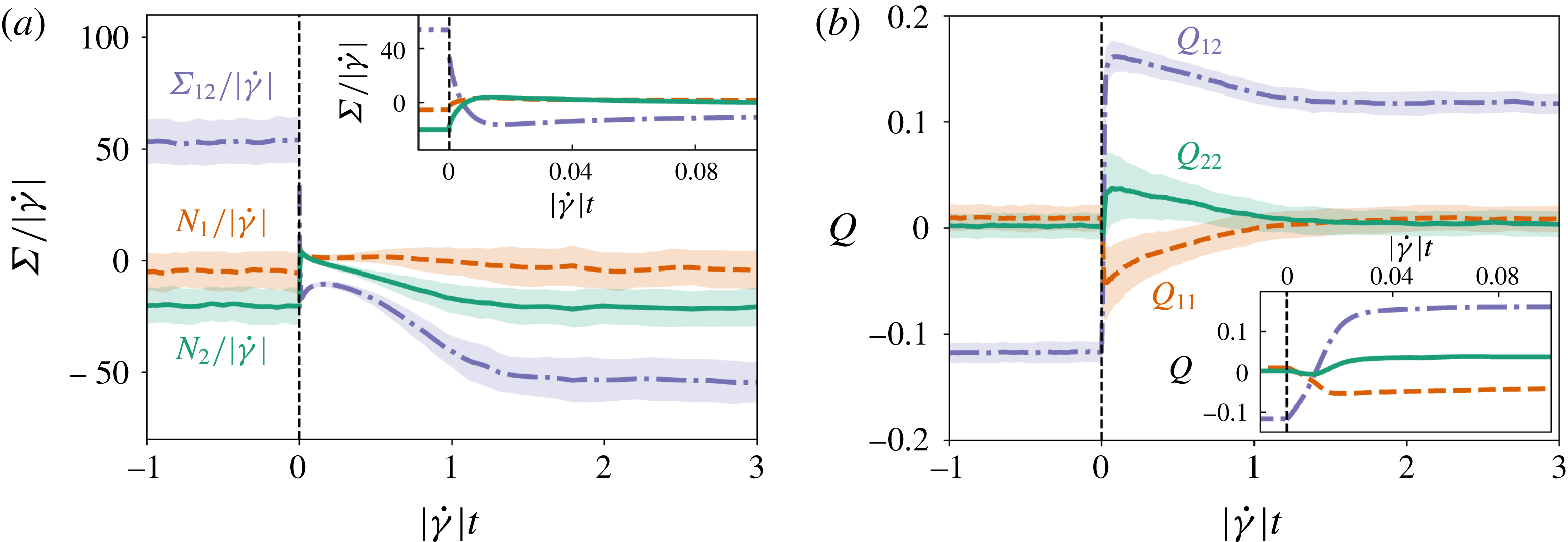
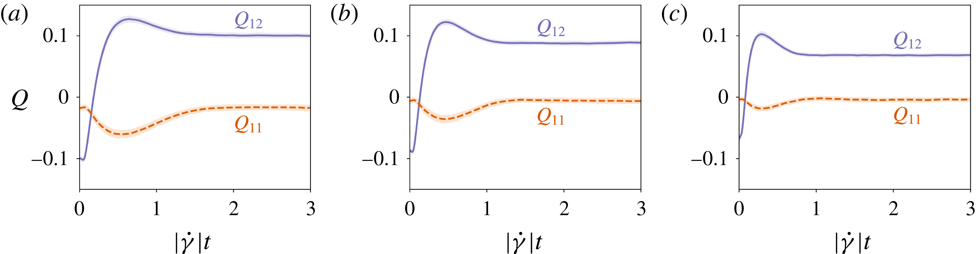
. In figure 1, we show that the dynamics of
 $\unicode[STIX]{x1D64C}^{\unicode[STIX]{x1D716}=0}$
(i.e. including only strict contacts, which correspond to interactions with a small negative gap thanks to the finite deformability of the particles) and
 $\unicode[STIX]{x1D72E}$
share several features upon reversal. In particular, they both show a discontinuity exactly at reversal, followed by a relaxation back to steady state over the same strain scale, here roughly 2 strain units for
 $\unicode[STIX]{x1D719}=0.5$
. (Strictly speaking, because of the slight deformability of the particles, the apparent discontinuity in
 $\unicode[STIX]{x1D64C}^{\unicode[STIX]{x1D716}=0}$
at reversal is actually a fast relaxation taking place during the first 1 % of strain after reversal; see figure 1(b) inset.) Because of the symmetry of the simple shear flow, both admit non-zero values only for their diagonal components and for their shear components in the velocity-gradient plane,
 $Q_{12}$
and
 $\unicode[STIX]{x1D6F4}_{12}$
. The steady-state values of these components have the same parity under strain reversal, with sign reversal for shear and none for the diagonal elements, providing further motivation for the use of
 $\unicode[STIX]{x1D64C}$
as a proxy for the microstructure in a constitutive model for the stress
 $\unicode[STIX]{x1D72E}$
.
Stress and fabric data from numerical simulations. (a) Stress tensor components
 $\unicode[STIX]{x1D6F4}_{12}$
,
 $N_{1}=\unicode[STIX]{x1D6F4}_{11}-\unicode[STIX]{x1D6F4}_{22}$
and
 $N_{2}=\unicode[STIX]{x1D6F4}_{22}-\unicode[STIX]{x1D6F4}_{33}$
divided by the absolute value of the shear rate
 $|\dot{\unicode[STIX]{x1D6FE}}|$
upon shear reversal at
 $\unicode[STIX]{x1D6FE}=0$
for
 $\unicode[STIX]{x1D719}=0.5$
. Components
 $\unicode[STIX]{x1D6F4}_{13}$
and
 $\unicode[STIX]{x1D6F4}_{23}$
are not shown, as they vanish in simple shear by symmetry. Thick dark-shaded lines are the averaged data, while the light shaded area around each curve is the standard deviation obtained from the individual shear reversals. All components show a discontinuity upon reversal, arising from lubrication and/or contact forces. (b) Fabric tensor components (with
 $\unicode[STIX]{x1D716}=0$
, describing full contacts only) for the same conditions, with averages in thick lines and standard deviation in shaded areas. Not shown are
 $Q_{13}=Q_{23}=0$
and
 $Q_{33}=-Q_{11}-Q_{22}$
. Insets: zoom-in on strains near the point of reversal.

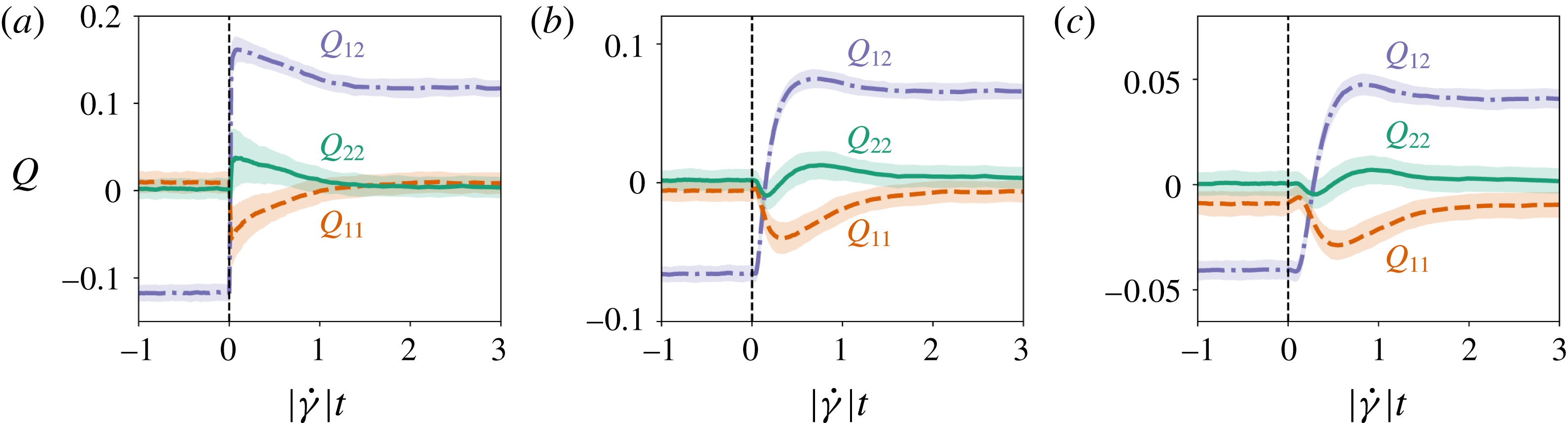
Fabric tensor components upon reversal at
 $\unicode[STIX]{x1D6FE}=0$
for
 $\unicode[STIX]{x1D719}=0.5$
and for three different cut-off lengths, (a)
 $\unicode[STIX]{x1D716}=0$
, (b)
 $\unicode[STIX]{x1D716}=0.02$
and (c)
 $\unicode[STIX]{x1D716}=0.1$
, from numerical simulations. The fabric tensor built on contacts (i.e. with
 $\unicode[STIX]{x1D716}=0$
(a)) is discontinuous upon reversal, as a finite fraction of contacts disappear when the flow is reversed. However, when the cut-off length is finite (i.e. (b) and (c)), the discontinuity disappears, and instead there is a delay followed by a rapid evolution of the
 $Q_{ij}$
from their pre-reversal steady-state values to their maximum (
 $Q_{12}$
and
 $Q_{22}$
) or minimum (
 $Q_{11}$
) values, both phases occurring over a strain of order
 $\unicode[STIX]{x1D716}$
.

However, despite the appeal of the similarity with the dynamics of the stress,
 $\unicode[STIX]{x1D64C}^{\unicode[STIX]{x1D716}=0}$
is discontinuous at reversal whereas solutions of (3.3) are continuous. In figure 2, we show instead that, for
 $\unicode[STIX]{x1D716}>0$
,
 $\unicode[STIX]{x1D64C}^{\unicode[STIX]{x1D716}}$
is continuous upon reversal and thus possibly described by an evolution like (3.3), and otherwise keeps most of the qualitative features of
 $\unicode[STIX]{x1D64C}^{\unicode[STIX]{x1D716}=0}$
. The initial singular reversal behaviour is smoothed over a finite strain scale which is increasing with
 $\unicode[STIX]{x1D716}$
and saturates for large
 $\unicode[STIX]{x1D716}$
to a strain
 $O(1)$
. Separately, the overall amplitude of
 $\unicode[STIX]{x1D64C}^{\unicode[STIX]{x1D716}}$
decreases with
 $\unicode[STIX]{x1D716}$
.
An appealing strategy is then to assume that knowledge of the fabric of near-contacts,
 $\unicode[STIX]{x1D64C}^{\unicode[STIX]{x1D716}>0}$
, along with knowledge of the flow itself, is enough to predict the evolution of the stress tensor
 $\unicode[STIX]{x1D72E}$
. That is, a continuous time evolution of
 $\unicode[STIX]{x1D64C}$
obeying an ODE in the Hand class might be married with a rule for constructing
 $\unicode[STIX]{x1D72E}(\unicode[STIX]{x1D64C},\unicode[STIX]{x1D646})$
that, through its dependence on
 $\unicode[STIX]{x1D646}$
, is explicitly alert to discontinuities at the moment of strain reversal. (This rule could build in information about the sudden opening of contacts on scales below
 $\unicode[STIX]{x1D716}$
, for instance.) An alternative strategy is to build a time evolution for the true contact fabric (
 $\unicode[STIX]{x1D716}=0$
) based on two relaxation times, one large corresponding to the time scale of reorganization of the microstructure, and one extremely small to describe the instantaneous changes in the contacts upon flow changes (Goddard Reference Goddard2006). However, with this approach, the fit to actual data imposes the parameters associated with the short time relaxation to take values whose physical interpretation is complex, including, for instance, transiently negative diffusion coefficients (Goddard Reference Goddard2008).
We stress that the cut-off length
 $\unicode[STIX]{x1D716}$
is not related to the lubrication regularization length
 $\unicode[STIX]{x1D6FF}$
nor to the maximum allowed overlap in the contact model. Moreover, it appears that, because
 $\unicode[STIX]{x1D64C}^{\unicode[STIX]{x1D716}}$
is getting smoothed out with increasing
 $\unicode[STIX]{x1D716}$
, the effects of contact overlaps and
 $\unicode[STIX]{x1D6FF}$
, which are only visible in particle trajectories at very early strains after reversal, will be gradually hidden in the time evolution of
 $\unicode[STIX]{x1D64C}^{\unicode[STIX]{x1D716}}$
for increasing
 $\unicode[STIX]{x1D716}$
. In practice, we find that
 $\unicode[STIX]{x1D64C}^{\unicode[STIX]{x1D716}}$
becomes insensitive to a doubling of
 $\unicode[STIX]{x1D6FF}$
for
 $\unicode[STIX]{x1D716}$
as small as 0.01. With this as the modelling strategy, picking the best cut-off length
 $\unicode[STIX]{x1D716}$
to build a constitutive model is then a compromise between the accuracy needed to admit a quantitative stress rule from
 $\unicode[STIX]{x1D64C}^{\unicode[STIX]{x1D716}}$
, and the smoothness required for an ODE closure in the
 $\unicode[STIX]{x1D64C}$
dynamics. In this work, we do not address the issue of the stress rule further, addressing solely the dynamics of
 $\unicode[STIX]{x1D64C}$
itself. We will focus our numerical tests of fabric evolution models on the case
 $\unicode[STIX]{x1D716}=0.02$
, adopting the default notation
 $\unicode[STIX]{x1D64C}:=\unicode[STIX]{x1D64C}^{\unicode[STIX]{x1D716}=0.02}$
. But, as shown in figures 2 and 3, the qualitative features of the dynamics are shared across all values of
 $\unicode[STIX]{x1D716}$
, so that most of what we will learn by trying to fit the case
 $\unicode[STIX]{x1D716}=0.02$
readily extends to other values of
 $\unicode[STIX]{x1D716}$
.
4.2 Weak anisotropy: small-
 $\unicode[STIX]{x1D64C}$
models

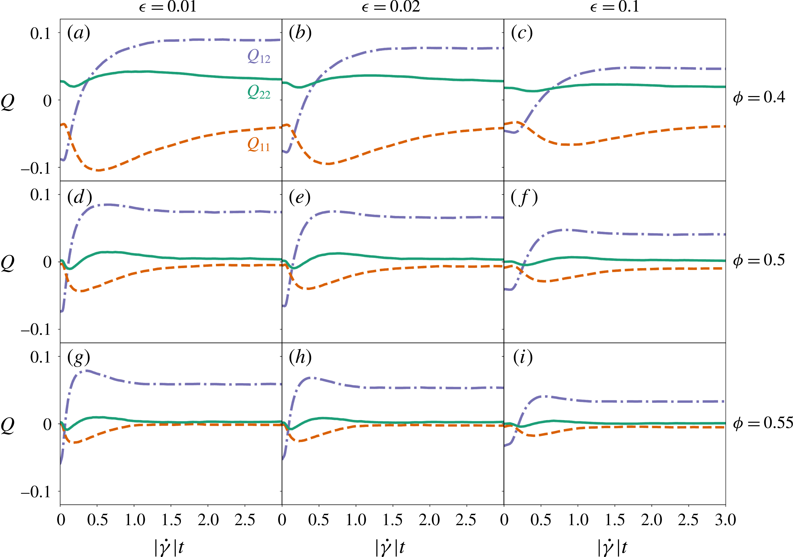
Fabric tensor components upon reversal at
 $\unicode[STIX]{x1D6FE}=0$
for three volume fractions,
 $\unicode[STIX]{x1D719}=0.4$
(a–c), 0.5 (d–f) and 0.55 (g–i), and for three different cut-off scales,
 $\unicode[STIX]{x1D716}=0.01$
(a,d,g), 0.02 (b,e,h) and 0.1 (c,f,i), from numerical simulations.

At large volume fractions, the steric constraints impose that every particle in the suspension is surrounded by close neighbours in any direction, with possibly only one direction (the compressional axis in simple shear) being slightly more crowded than the others. We can then expect that the anisotropy of the microstructure is decreasing with increasing
 $\unicode[STIX]{x1D719}$
.
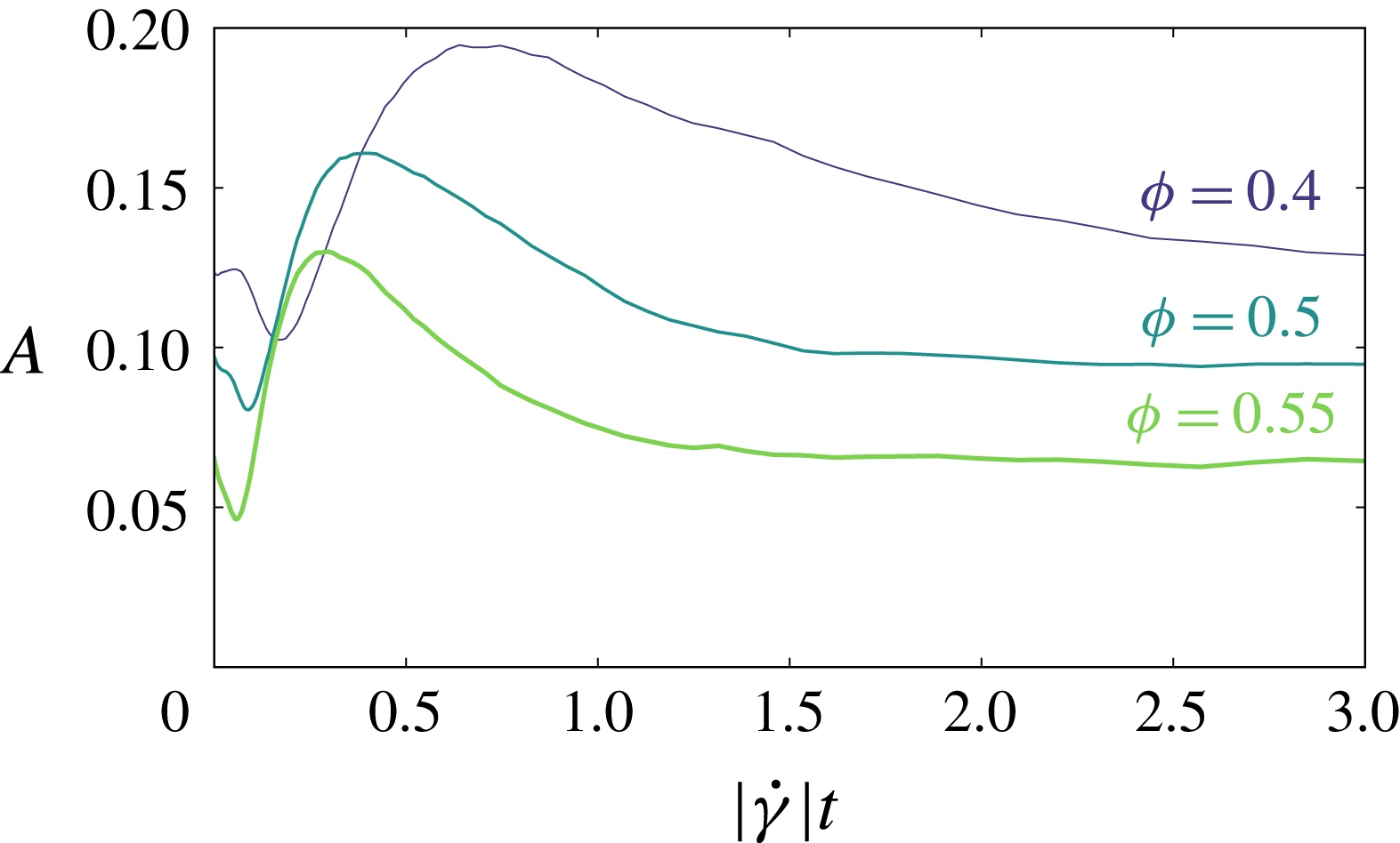
Anisotropy
 $A$
as a function of post-reversal strain for three volume fractions,
 $\unicode[STIX]{x1D719}=0.4$
, 0.5 and 0.55, from numerical simulations.

As evidence for this, given a distribution of near-contacts
 $P(\boldsymbol{p})$
, we quantify its anisotropy by defining
 $A:=(4\unicode[STIX]{x03C0})^{-1}\int _{S^{2}}[4\unicode[STIX]{x03C0}P(\boldsymbol{p})-1]^{2}\,\text{d}\unicode[STIX]{x1D6FA}$
. Figure 4 shows the post-reversal evolution of
 $A$
for various volume fractions
 $\unicode[STIX]{x1D719}$
, and makes it clear that
 $A$
does indeed decrease with increasing
 $\unicode[STIX]{x1D719}$
. Similarly, in figure 3, we show the dependence of
 $\unicode[STIX]{x1D64C}$
on
 $\unicode[STIX]{x1D719}$
, for several values of
 $\unicode[STIX]{x1D716}$
, which demonstrates for
 $\unicode[STIX]{x1D64C}$
the corresponding lowering of the anisotropy as
 $\unicode[STIX]{x1D719}$
increases. To quantify further how small
 $\unicode[STIX]{x1D64C}$
actually is, we can look at a norm such as
 $|\unicode[STIX]{x1D64C}|=\sqrt{\text{Tr}[\unicode[STIX]{x1D64C}^{2}]}$
. It is easy to show that
 $|\unicode[STIX]{x1D64C}|\leqslant \sqrt{2/3}\approx 0.816$
, with equality corresponding to having all the
 $\boldsymbol{p}$
in the same direction,
 $P(\boldsymbol{p})=\unicode[STIX]{x1D6FF}(\boldsymbol{p}-\boldsymbol{p}_{0})$
. In contrast with this saturation value, we observe in steady state for
 $\unicode[STIX]{x1D719}=0.4$
and
 $\unicode[STIX]{x1D716}=0.01$
(figure 3
a),
 $|\unicode[STIX]{x1D64C}|\approx 0.048$
, and for
 $\unicode[STIX]{x1D719}=0.55$
and
 $\unicode[STIX]{x1D716}=0.01$
(figure 3
g),
 $|\unicode[STIX]{x1D64C}|\approx 0.0022$
. These numbers, which confirm a weak anisotropy limit, become even smaller if we increase
 $\unicode[STIX]{x1D716}$
. A reasonable assumption, based on the smallness of these values, is to restrict the evolution equation (3.3) to low orders in
 $\unicode[STIX]{x1D64C}$
, allowing a Taylor expansion of the dynamics around the isotropic state. In what follows, we will examine the resulting dynamical equations at successively higher orders in
 $\unicode[STIX]{x1D64C}$
.
4.3 Hand equation in simple shear
From now on, we restrict our discussion to a simple shear flow with
 $\hat{K}_{ij}=0$
except
 $\hat{K}_{12}=\pm 1/2$
, which is the simulation case. Because of the sparsity of
 $\hat{\unicode[STIX]{x1D646}}$
in this geometry, not all the components on the right-hand side of (3.3) are linearly independent, and some of the
 $\unicode[STIX]{x1D6FC}_{i}$
are redundant. Hence we recast the tensorial Hand equation for rate-independent systems (3.3) in a non-redundant component form (see appendix B) as
 $$\begin{eqnarray}\displaystyle \left.\begin{array}{@{}c@{}}\dot{Q}_{-}=P_{-}[Q_{+},\operatorname{sgn}(\dot{\unicode[STIX]{x1D6FE}})Q_{12},Q_{-}^{2}]\operatorname{sgn}(\dot{\unicode[STIX]{x1D6FE}})Q_{-}+2Q_{12},\\ \dot{Q}_{+}=P_{+}[Q_{+},\operatorname{sgn}(\dot{\unicode[STIX]{x1D6FE}})Q_{12},Q_{-}^{2}]\operatorname{sgn}(\dot{\unicode[STIX]{x1D6FE}}),\\ \dot{Q}_{12}=P_{12}[Q_{+},\operatorname{sgn}(\dot{\unicode[STIX]{x1D6FE}})Q_{12},Q_{-}^{2}]-\frac{1}{2}Q_{-},\end{array}\right\} & & \displaystyle\end{eqnarray}$$
with functions
 $P_{-}$
,
 $P_{+}$
and
 $P_{12}$
analytic in their arguments, where
 $Q_{\pm }:=Q_{11}\pm Q_{22}$
.
We see from (4.2) that, when fitting these equations to simulation data, the basis of choice is
 $\{Q_{+},Q_{-},Q_{12}\}$
, rather than the naive basis
 $\{Q_{11},Q_{22},Q_{12}\}$
. Choosing the
 $\{Q_{+},Q_{-},Q_{12}\}$
basis when plotting fits has the effect of highlighting the important features of the data that a given model is trying to fit. For reversal protocols in particular, apparent qualitative agreement between model and data for
 $Q_{11}(\unicode[STIX]{x1D6FE})$
and
 $Q_{22}(\unicode[STIX]{x1D6FE})$
can be exposed as clear disagreement in this basis.
5 Linear and quadratic Hand equations
5.1 Linear Hand equation
We begin by assuming the fabric evolves via a frame-indifferent ODE linear in
 $\unicode[STIX]{x1D64C}$
. From (3.2), the most general linear model is
 $$\begin{eqnarray}\displaystyle \operatorname{sgn}(\dot{\unicode[STIX]{x1D6FE}})\dot{\unicode[STIX]{x1D64C}} & = & \displaystyle \hat{\unicode[STIX]{x1D652}}\boldsymbol{\cdot }\unicode[STIX]{x1D64C}-\unicode[STIX]{x1D64C}\boldsymbol{\cdot }\hat{\unicode[STIX]{x1D652}}+\unicode[STIX]{x1D6FC}_{1}\unicode[STIX]{x1D64C}+\unicode[STIX]{x1D6FC}_{2}\hat{\unicode[STIX]{x1D640}}+\unicode[STIX]{x1D6FC}_{4}\hat{\unicode[STIX]{x1D640}}^{2}\nonumber\\ \displaystyle & & \displaystyle +\,\unicode[STIX]{x1D6FC}_{5}(\hat{\unicode[STIX]{x1D640}}\boldsymbol{\cdot }\unicode[STIX]{x1D64C}+\unicode[STIX]{x1D64C}\boldsymbol{\cdot }\hat{\unicode[STIX]{x1D640}})+\unicode[STIX]{x1D6FC}_{7}(\hat{\unicode[STIX]{x1D640}}^{2}\boldsymbol{\cdot }\unicode[STIX]{x1D64C}+\unicode[STIX]{x1D64C}\boldsymbol{\cdot }\hat{\unicode[STIX]{x1D640}}^{2})\nonumber\\ \displaystyle & & \displaystyle -\,{\textstyle \frac{1}{3}}(\unicode[STIX]{x1D6FC}_{4}\hat{I} _{5}+2\unicode[STIX]{x1D6FC}_{5}\hat{I} _{7}+2\unicode[STIX]{x1D6FC}_{7}\hat{I} _{9})\unicode[STIX]{x1D644},\end{eqnarray}$$
with
 $$\begin{eqnarray}\displaystyle \left.\begin{array}{@{}c@{}}\unicode[STIX]{x1D6FC}_{1}=x_{10},\\ \unicode[STIX]{x1D6FC}_{2}=x_{20}+x_{27}\hat{I} _{7}+x_{29}\hat{I} _{9},\\ \unicode[STIX]{x1D6FC}_{4}=x_{40}+x_{47}\hat{I} _{7}+x_{49}\hat{I} _{9},\\ \unicode[STIX]{x1D6FC}_{5}=x_{50},\\ \unicode[STIX]{x1D6FC}_{7}=x_{70},\end{array}\right\} & & \displaystyle\end{eqnarray}$$
in which we denote by
 $x_{ij}$
the constant coefficients in
 $\unicode[STIX]{x1D6FC}_{i}$
in front of
 $\hat{I} _{j}$
(with the exception of
 $x_{i0}$
, which comes alone). We recall that
 $\hat{I} _{5}=\text{Tr}[\hat{\unicode[STIX]{x1D640}}^{2}]$
,
 $\hat{I} _{7}=\text{Tr}[\unicode[STIX]{x1D64C}\boldsymbol{\cdot }\hat{\unicode[STIX]{x1D640}}]$
and
 $\hat{I} _{9}=\text{Tr}[\unicode[STIX]{x1D64C}\boldsymbol{\cdot }\hat{\unicode[STIX]{x1D640}}^{2}]$
.
As previously indicated, in simple shear flow, not all of the
 $x_{ij}$
can be separately tested against numerics. In the non-redundant componentwise basis (4.2), the linear model corresponds to functions
 $P_{-}$
,
 $P_{+}$
and
 $P_{12}$
of the form
 $$\begin{eqnarray}\displaystyle \left.\begin{array}{@{}c@{}}P_{-}=a_{-},\\ P_{+}=a_{+}+b_{+}Q_{+}+c_{+}\operatorname{sgn}(\dot{\unicode[STIX]{x1D6FE}})Q_{12},\\ P_{12}=a_{12}+b_{12}Q_{+}+c_{12}\operatorname{sgn}(\dot{\unicode[STIX]{x1D6FE}})Q_{12},\end{array}\right\} & & \displaystyle\end{eqnarray}$$
where we have introduced seven independent constants (the
 $a$
,
 $b$
and
 $c$
).
Interestingly, this model is strongly constrained for the dynamics of
 $Q_{-}$
. More precisely, we now establish that equations (4.2) and (5.3) imply a rigorous condition on the post-reversal behaviour of
 $Q_{-}$
. After reversal,
 $\unicode[STIX]{x1D64C}$
reaches a steady-state value
 $\unicode[STIX]{x1D64C}^{+SS}$
whose components, from (4.2) and (5.3), satisfy
 $$\begin{eqnarray}\displaystyle 0=a_{-}\operatorname{sgn}(\dot{\unicode[STIX]{x1D6FE}})Q_{-}^{+SS}+2Q_{12}^{+SS}. & & \displaystyle\end{eqnarray}$$
Subtracting this from the first line of (4.2) and defining
 $\unicode[STIX]{x0394}\unicode[STIX]{x1D64C}:=\unicode[STIX]{x1D64C}-\unicode[STIX]{x1D64C}^{+SS}$
, we get
 $$\begin{eqnarray}\displaystyle \unicode[STIX]{x0394}\dot{Q}_{-}=a_{-}\operatorname{sgn}(\dot{\unicode[STIX]{x1D6FE}})\unicode[STIX]{x0394}Q_{-}+2\unicode[STIX]{x0394}Q_{12}. & & \displaystyle\end{eqnarray}$$
Using the property of the pre-reversal steady state that
 $Q_{-}(\unicode[STIX]{x1D6FE}=0)=Q_{-}^{-SS}=Q_{-}^{+SS}$
, this can be integrated as
 $$\begin{eqnarray}\displaystyle \unicode[STIX]{x0394}Q_{-}(\unicode[STIX]{x1D6FE})=2\int _{0}^{\unicode[STIX]{x1D6FE}}\text{e}^{a_{-}\operatorname{sgn}(\dot{\unicode[STIX]{x1D6FE}})[\unicode[STIX]{x1D6FE}-\unicode[STIX]{x1D6FE}^{\prime }]}\unicode[STIX]{x0394}Q_{12}(\unicode[STIX]{x1D6FE}^{\prime })\,\text{d}\unicode[STIX]{x1D6FE}^{\prime }. & & \displaystyle\end{eqnarray}$$
From this, we can see in particular that, until
 $\unicode[STIX]{x0394}Q_{12}(\unicode[STIX]{x1D6FE})$
changes sign, the sign of
 $\unicode[STIX]{x0394}Q_{-}(\unicode[STIX]{x1D6FE})$
has to stay the same as
 $\operatorname{sgn}(\dot{\unicode[STIX]{x1D6FE}})\operatorname{sgn}(\unicode[STIX]{x0394}Q_{12}(0))$
, irrespective of the values of the
 $a$
,
 $b$
and
 $c$
coefficients. This constraint is a strong prediction for any linear model that can be easily compared with the numerical data.
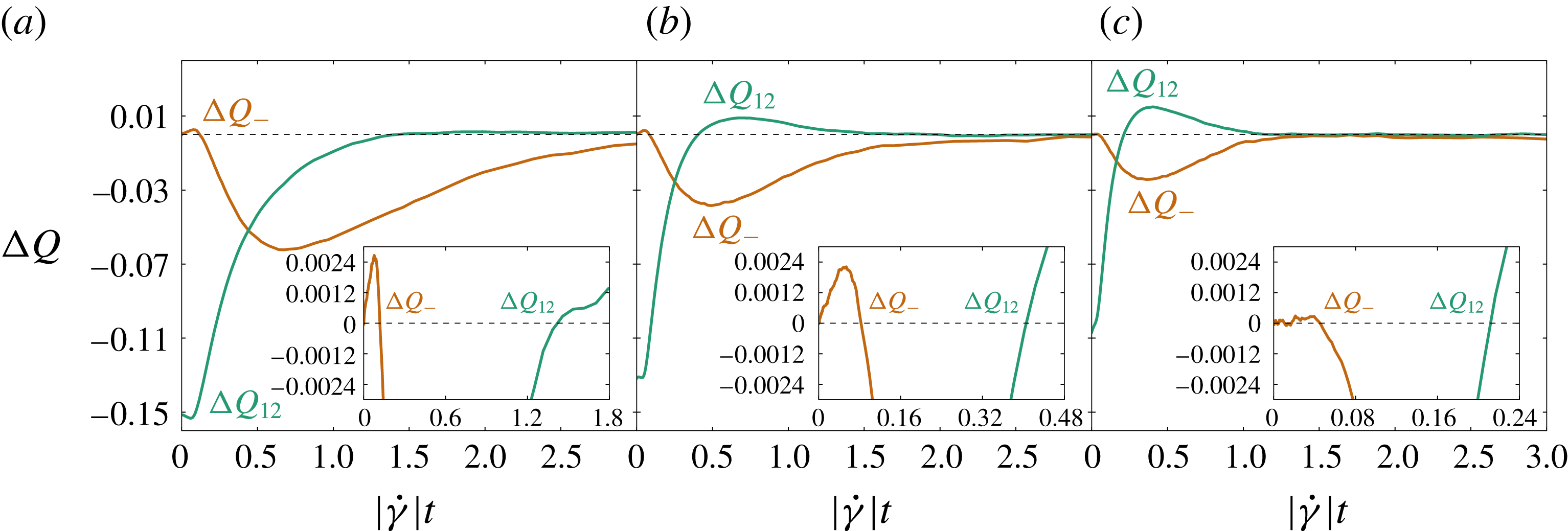
Simulation data for
 $\unicode[STIX]{x0394}Q_{-}$
and
 $\unicode[STIX]{x0394}Q_{12}$
against post-reversal strain for three volume fractions, (a)
 $\unicode[STIX]{x1D719}=0.4$
, (b)
 $\unicode[STIX]{x1D719}=0.5$
and (c)
 $\unicode[STIX]{x1D719}=0.55$
. Any fabric evolution model that is linear in the fabric itself predicts that
 $\unicode[STIX]{x0394}Q_{-}$
cannot change sign before
 $\unicode[STIX]{x0394}Q_{12}$
does, from (5.6). This condition is unambiguously violated for all of our simulation data. Insets: zoom-in on the region where the condition is violated.

Figure 5 shows the post-reversal evolution of
 $\unicode[STIX]{x0394}Q_{-}$
and
 $\unicode[STIX]{x0394}Q_{12}$
for the three volume fractions we investigated. In every case,
 $\unicode[STIX]{x0394}Q_{-}$
changes sign long before
 $\unicode[STIX]{x0394}Q_{12}$
. We moreover verified that this behaviour is observed for any cut-off length
 $\unicode[STIX]{x1D716}$
. This allows us to conclude that no linear model can yield a good fit to the data. This is the first important conclusion of our work. We are not aware of any similar rejection of linear fabric evolution models in previous work that does not address strain reversal.
Beyond ruling out the possibility of finding a suitable linear model, the simulations allow us to conduct diagnostics, identifying the source of the difficulty. Between
 $\unicode[STIX]{x1D6FE}$
and
 $\unicode[STIX]{x1D6FE}+\text{d}\unicode[STIX]{x1D6FE}$
,
 $\unicode[STIX]{x1D64C}$
evolves through three distinct processes: the advection of pairs of particles with separation
 $h<\unicode[STIX]{x1D716}$
; the birth of near-contacts counted in
 $\unicode[STIX]{x1D64C}$
when a pair of particles has separation
 $h>\unicode[STIX]{x1D716}$
at strain
 $\unicode[STIX]{x1D6FE}$
but
 $h<\unicode[STIX]{x1D716}$
an interval
 $\unicode[STIX]{x1D6FE}+\text{d}\unicode[STIX]{x1D6FE}$
later; and the death of near-contacts in the opposite case. Writing
 $r^{b}$
and
 $r^{d}$
for respectively the rate of near-contact births and deaths per near-contact,
 $\unicode[STIX]{x1D64C}^{b}$
and
 $\unicode[STIX]{x1D64C}^{d}$
for the fabric of near-contact births and deaths, and
 $\dot{\unicode[STIX]{x1D64C}}^{a}$
for the rate of change of
 $\unicode[STIX]{x1D64C}$
due to the advection of near-contacts not instantaneously being born or dying, we have (see appendix C)
 $$\begin{eqnarray}\displaystyle \dot{\unicode[STIX]{x1D64C}}=\dot{\unicode[STIX]{x1D64C}}^{a}+r^{b}\unicode[STIX]{x1D64C}^{b}-r^{d}\unicode[STIX]{x1D64C}^{d}. & & \displaystyle\end{eqnarray}$$
Instead of considering directly
 $\dot{\unicode[STIX]{x1D64C}}$
as a function of
 $\unicode[STIX]{x1D64C}$
, we can consider each term
 $\dot{\unicode[STIX]{x1D64C}}^{a}$
,
 $r^{b}\unicode[STIX]{x1D64C}^{b}$
and
 $r^{d}\unicode[STIX]{x1D64C}^{d}$
separately as functions of
 $\unicode[STIX]{x1D64C}$
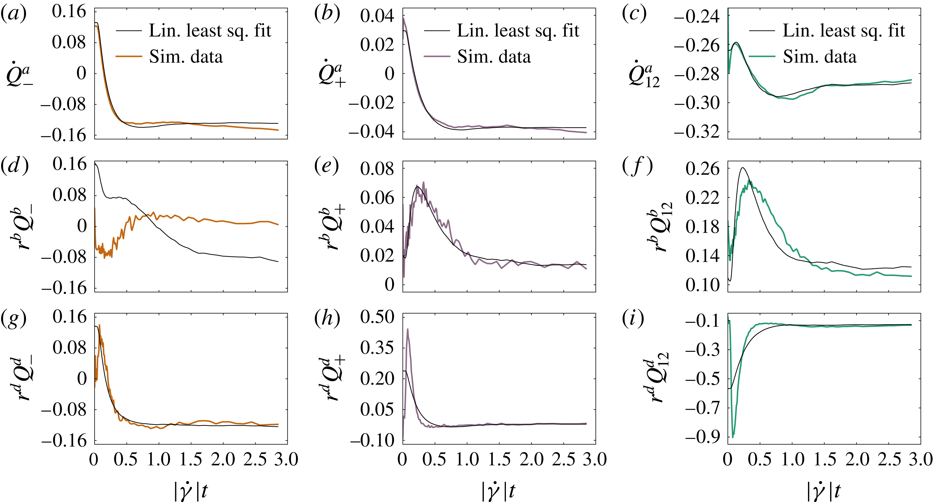
. Trying to fit, using linear least squares,
 $\dot{\unicode[STIX]{x1D64C}}^{a}$
as a function of
 $\unicode[STIX]{x1D64C}$
from simulation data with the linear model in (4.2), we obtain an excellent result, shown in figure 6(a–c). This implies that the need for a nonlinear model is not due to the advective part of the evolution, but rather due to the birth and death of near-contacts. This is confirmed in figure 6(d–i), showing that the linear model fails for both the birth and death contributions, and gives particularly bad results when the birth and death contributions take their largest values in amplitude, i.e. when good accuracy matters most.
The three
 $\dot{\unicode[STIX]{x1D64C}}$
contributions,
 $\dot{\unicode[STIX]{x1D64C}}^{a}$
(a–c),
 $r^{b}\unicode[STIX]{x1D64C}^{b}$
(d–f) and
 $r^{d}\unicode[STIX]{x1D64C}^{d}$
(g–i), as defined by (5.7), as functions of strain. For each contribution the three independent components
 $\dot{Q}_{-}^{a}$
,
 $\dot{Q}_{+}^{a}$
and
 $\dot{Q}_{12}^{a}$
(respectively,
 $r^{b}\unicode[STIX]{x1D64C}_{-}^{b}$
,
 $r^{b}\unicode[STIX]{x1D64C}_{+}^{b}$
and
 $r^{b}\unicode[STIX]{x1D64C}_{12}^{b}$
, and
 $r^{d}\unicode[STIX]{x1D64C}_{-}^{d}$
,
 $r^{d}\unicode[STIX]{x1D64C}_{+}^{d}$
and
 $r^{d}\unicode[STIX]{x1D64C}_{12}^{d}$
) are shown respectively in (a,d,g), (b,e,h) and (c,f,i) (black lines). Each component is compared to a fit to the linear model (5.3) (colour lines).

5.2 Quadratic Hand equation
Having ruled out the possibility of an adequate linear model, we consider the general quadratic model
 $$\begin{eqnarray}\displaystyle \left.\begin{array}{@{}c@{}}P_{-}=a_{-}+b_{-}Q_{+}+c_{-}\operatorname{sgn}(\dot{\unicode[STIX]{x1D6FE}})Q_{12},\\ P_{+}=a_{+}+b_{+}Q_{+}+c_{+}\operatorname{sgn}(\dot{\unicode[STIX]{x1D6FE}})Q_{12}+d_{+}Q_{+}^{2}+e_{+}Q_{12}^{2}+f_{+}Q_{-}^{2},\\ P_{12}=a_{12}+b_{12}Q_{+}+c_{12}\operatorname{sgn}(\dot{\unicode[STIX]{x1D6FE}})Q_{12}+d_{12}Q_{+}^{2}+e_{12}Q_{12}^{2}+f_{12}Q_{-}^{2}.\end{array}\right\} & & \displaystyle\end{eqnarray}$$
The parameter space of this model, with 15 dimensions, is difficult to explore. The strategy we adopt can be found in § 5.1 of Cheng, Jia & Wang (Reference Cheng, Jia and Wang2007), and is to numerically differentiate
 $\unicode[STIX]{x1D64C}$
(see appendix C), and use linear least squares to fit these quadratic models, with
 $\unicode[STIX]{x1D64C}$
taken from simulation data, to
 $\dot{\unicode[STIX]{x1D64C}}$
. The logic behind this is that, if the model is capable of yielding a good qualitative fit to
 $\unicode[STIX]{x1D64C}$
, it will also provide an adequate fit to
 $\dot{\unicode[STIX]{x1D64C}}$
, particularly if the fit is quantitatively good as well.
This approach very often fails for quadratic models governed by (5.8), because the parameter set obtained in this way may, when used to evolve
 $\unicode[STIX]{x1D64C}$
from its initial condition, cause
 $\unicode[STIX]{x1D64C}$
to grow unbounded. It is easy to see why: quadratic models correspond to the overdamped dynamics of a three-dimensional vector
 $\boldsymbol{s}=\{Q_{-},Q_{+},Q_{12}\}$
in a cubic potential
 ${\dot{s}}_{i}=-\unicode[STIX]{x1D735}_{s_{i}}[A_{jkl}s_{j}s_{k}s_{l}+B_{jk}s_{j}s_{k}+C_{k}s_{k}]$
, with
 $\unicode[STIX]{x1D63C}$
,
 $\unicode[STIX]{x1D63D}$
and
 $\unicode[STIX]{x1D63E}$
tensors depending on the coefficients of (5.8). A cubic potential is generically not confining, so that unless the initial conditions are within the basin of attraction of a local potential minimum,
 $\boldsymbol{s}$
will grow unbounded. Finding a well-behaved quadratic fabric evolution model then involves identifying parameters for which
 $\{Q_{-}^{-SS},Q_{+}^{-SS},Q_{12}^{-SS}\}$
lies within such a basin. This appears to be an unsatisfactory approach at best.
By setting some parameters of (5.8) to zero, it is possible to restrict the parameter space enough to find a model with a bounded evolution. For instance, the best quadratic model we could find takes the form
 $$\begin{eqnarray}\displaystyle \left.\begin{array}{@{}c@{}}P_{-}=a_{-}+b_{-}Q_{+}+c_{-}\operatorname{sgn}(\dot{\unicode[STIX]{x1D6FE}})Q_{12},\\ P_{+}=a_{+}+b_{+}Q_{+}+c_{+}\operatorname{sgn}(\dot{\unicode[STIX]{x1D6FE}})Q_{12}+e_{+}Q_{12}^{2},\\ P_{12}=a_{12}+b_{12}Q_{+}+c_{12}\operatorname{sgn}(\dot{\unicode[STIX]{x1D6FE}})Q_{12}+e_{12}Q_{12}^{2}.\end{array}\right\} & & \displaystyle\end{eqnarray}$$
This contains 11 free parameters, which we fit initially by linear least squares on (4.2), that is, minimizing over the parameters
 $a_{-}$
,
 $b_{-}$
,
 $c_{-}$
,
 $a_{+}$
,
 $b_{+}$
,
 $c_{+}$
,
 $e_{+}$
,
 $a_{12}$
,
 $b_{12}$
,
 $c_{12}$
and
 $e_{12}$
the quantity
 $$\begin{eqnarray}\displaystyle X_{1} & = & \displaystyle \int _{\unicode[STIX]{x1D6FE}=0}^{\unicode[STIX]{x1D6FE}=3}\{(\dot{Q}_{-}^{data}-P_{-}[Q_{+}^{data},\operatorname{sgn}(\dot{\unicode[STIX]{x1D6FE}})Q_{12}^{data},Q_{-}^{2\,data}]\operatorname{sgn}(\dot{\unicode[STIX]{x1D6FE}})Q_{-}^{data}-2Q_{12}^{data})^{2}\nonumber\\ \displaystyle & & \displaystyle +\,(\dot{Q}_{+}^{data}-P_{+}[Q_{+}^{data},\operatorname{sgn}(\dot{\unicode[STIX]{x1D6FE}})Q_{12}^{data},Q_{-}^{2\,data}]\operatorname{sgn}(\dot{\unicode[STIX]{x1D6FE}}))^{2}\nonumber\\ \displaystyle & & \displaystyle +(\dot{Q}_{12}^{data}-P_{12}[Q_{+}^{data},\operatorname{sgn}(\dot{\unicode[STIX]{x1D6FE}})Q_{12}^{data},Q_{-}^{2\,data}]+{\textstyle \frac{1}{2}}Q_{-}^{data})^{2}\!\}\,\text{d}\unicode[STIX]{x1D6FE}\end{eqnarray}$$
with strain series
 $\unicode[STIX]{x1D64C}^{data}$
and
 $\dot{\unicode[STIX]{x1D64C}}^{data}$
taken from the simulation data. Note that there is some freedom in choosing the upper
 $\unicode[STIX]{x1D6FE}$
limit in the integral of (5.10); a larger maximum
 $\unicode[STIX]{x1D6FE}$
will favour fits that are accurate in steady state, while a smaller one will favour good accuracy in the early phase. The value
 $\unicode[STIX]{x1D6FE}=3$
picked here is the one that we found to give the most balanced results between the two extremes. After this initial fit, we further apply a gradient descent to minimize the linear least squares between the actual model prediction
 $\unicode[STIX]{x1D64C}^{fit}$
(obtained by integrating equation (4.2) over strain with initial conditions from the simulation data
 $\unicode[STIX]{x1D64C}^{data}(\unicode[STIX]{x1D6FE}=0)$
) and the numerical data
 $\unicode[STIX]{x1D64C}^{data}$
, that is, minimizing
 $$\begin{eqnarray}\displaystyle X_{2}=\int _{\unicode[STIX]{x1D6FE}=0}^{\unicode[STIX]{x1D6FE}=3}[(Q_{-}^{fit}-Q_{-}^{data})^{2}+(Q_{+}^{fit}-Q_{+}^{data})^{2}+(Q_{12}^{fit}-Q_{12}^{data})^{2}]\,\text{d}\unicode[STIX]{x1D6FE} & & \displaystyle\end{eqnarray}$$
to get final best-fit parameters.
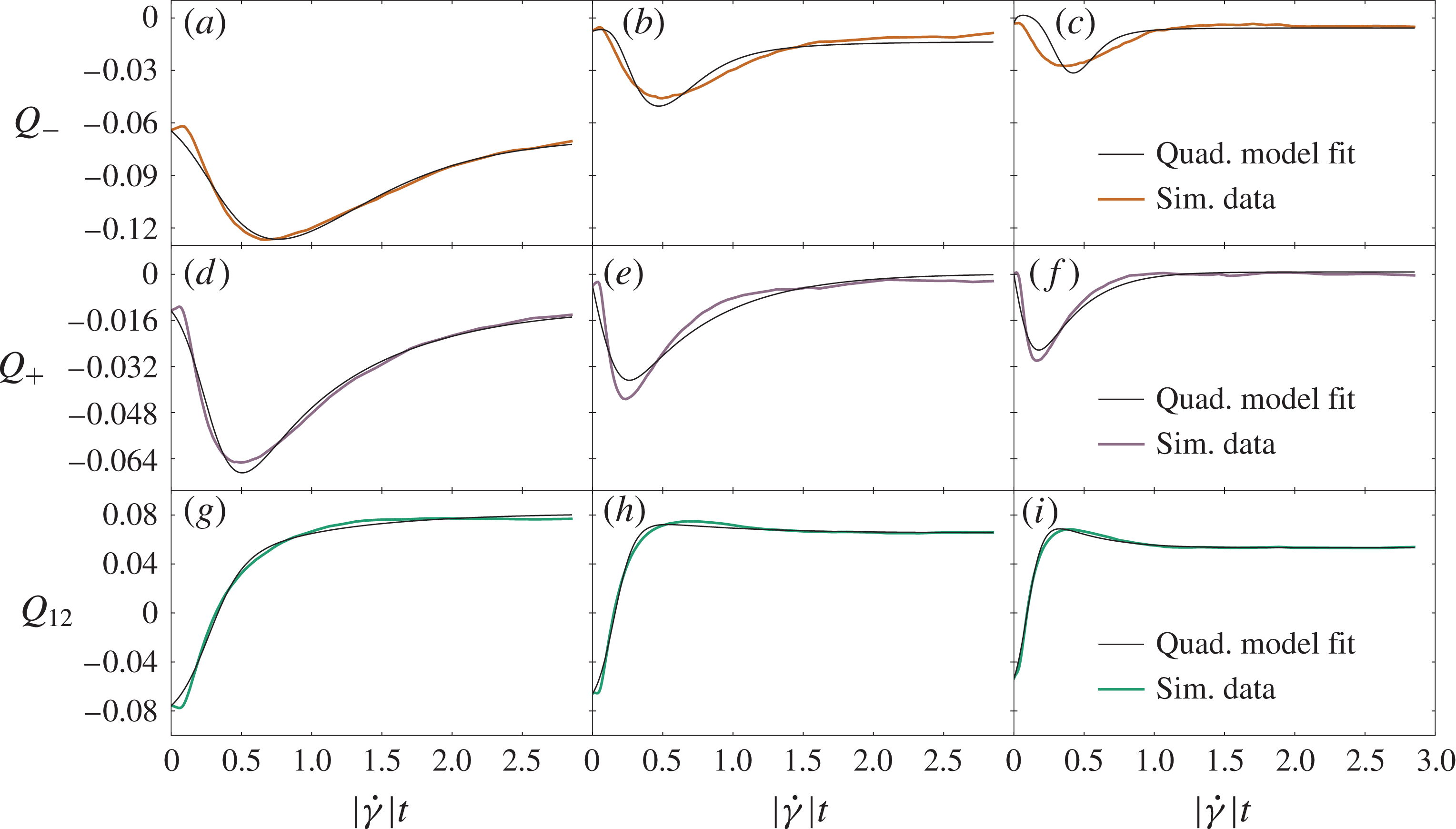
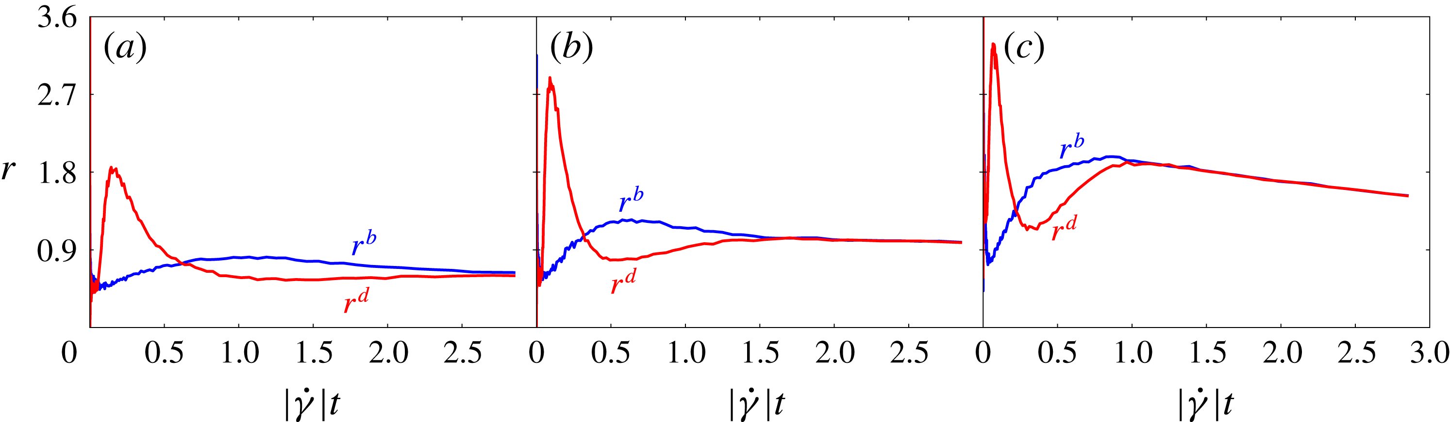
Depending on the component of interest, this procedure leads to fits ranging from good to excellent, as shown in figure 7. The only obvious weakness is a moderate but increasing discrepancy for
 $Q_{-}$
when
 $\unicode[STIX]{x1D719}$
increases. This is probably due to the smaller
 $r^{b}$
and
 $r^{d}$
at low volume fraction (see figure 8), yielding flatter, easier-to-fit curves.
Fits of the quadratic model described by (5.9) to simulation data for the three components of
 $\unicode[STIX]{x1D64C}$
(respectively,
 $Q_{-}$
,
 $Q_{+}$
and
 $Q_{12}$
from a–i) against post-reversal strain for
 $\unicode[STIX]{x1D719}=0.4$
(a,d,g),
 $\unicode[STIX]{x1D719}=0.5$
(b,e,h) and
 $\unicode[STIX]{x1D719}=0.55$
(c,f,i).

Simulation data for the fractional birth rate
 $r^{b}$
(blue) and death rate
 $r^{d}$
(red) against post-reversal strain for (a)
 $\unicode[STIX]{x1D719}=0.4$
, (b)
 $\unicode[STIX]{x1D719}=0.5$
and (c)
 $\unicode[STIX]{x1D719}=0.55$
.

Because of the difficulty to find a well-behaved model, we cannot perform a thorough exploration of parameter space, and there may be a better-fitting quadratic model than (5.9). In any case the fitting power of quadratic models is, in three dimensions, in principle satisfactory when it comes to matching the numerically observed fabric evolution. However, we believe this to be largely coincidental, rather than faithful to the underlying physics, and stemming simply from the large number of parameters available. This is partly because there is no reason to expect the parameters of a mechanistically faithful model to need fine-tuning to avoid the generic blow-up described previously. However, a stronger reason to reject such models is found by making a detour to the two-dimensional case, as we describe next.
6 Insights from the two-dimensional case
As we have shown in § 5, linear models do not contain enough physics to capture the relation between the post-reversal dynamics of
 $Q_{-}$
and
 $Q_{12}$
, that is, the dynamics in the shear plane. Quadratic models are able to achieve a quantitative fit to
 $Q_{-}$
and
 $Q_{12}$
, but at the price of a greatly increased number of free parameters, which, coupled with the generic presence of instabilities, suggests that the difficulty has been circumvented simply by over-parametrizing the problem. To understand better what is the source of the difficulty, we can consider the simplified case of a two-dimensional suspension, for which by construction the shear plane dynamics can be described in isolation, with the hope that it shares its characteristic features with the three-dimensional case.
Fabric tensor components upon reversal at
 $|\dot{\unicode[STIX]{x1D6FE}}|t=0$
for (a)
 $\unicode[STIX]{x1D719}=0.65$
, (b)
 $\unicode[STIX]{x1D719}=0.7$
and (c)
 $\unicode[STIX]{x1D719}=0.75$
in two-dimensional numerical simulations. As in three dimensions,
 $\unicode[STIX]{x1D64C}$
flips on a strain scale of order 1, there is an overshoot in
 $Q_{12}$
and
 $Q_{-}$
(
 $=2Q_{11}$
in two dimensions) is negative. Also,
 $\unicode[STIX]{x1D64C}$
gets smaller and flips on a shorter strain scale as
 $\unicode[STIX]{x1D719}$
increases. Thick dark-shaded lines are the averaged data, while the light shaded area around each curve is the standard deviation obtained from the individual shear reversals. Note that the variance of the individual runs appears smaller here than in the three-dimensional case in figure 2. This is the result of using larger system sizes in two dimensions (
 $N=4000$
) than in three (
 $N=500$
).

Thus, in this section we perform numerical simulations of a two-dimensional monolayer of spheres, and we try to model the evolution of the fabric tensor, as before. The simulation technique is the same as in three dimensions, only with a different number of particles
 $N=4000$
and different area fractions
 $\unicode[STIX]{x1D719}=0.65$
, 0.7 and 0.75. Also, the average results for the fabric tensor are obtained over 100 shear reversal realizations.
In two dimensions, the fabric tensor
 $\unicode[STIX]{x1D64C}:=\langle \boldsymbol{p}\boldsymbol{p}\rangle -{\textstyle \frac{1}{2}}\unicode[STIX]{x1D644}$
reduces to two independent non-zero components
 $Q_{12}$
and
 $Q_{-}=2Q_{11}=-2Q_{22}$
. The fabric evolution in two dimensions is shown in figure 9 for
 $\unicode[STIX]{x1D719}=0.65$
, 0.7 and 0.75. Comparing these data with the three-dimensional ones shown in figure 3, we can see that the qualitative behaviour is the same in two and three dimensions, and we can thus gain insight from the simplified two-dimensional case.
The two-dimensional version of the system of ODEs (4.2) is (see appendix B)
 $$\begin{eqnarray}\displaystyle \left.\begin{array}{@{}c@{}}\dot{Q}_{-}=P_{-}[\operatorname{sgn}(\dot{\unicode[STIX]{x1D6FE}})Q_{12},Q_{-}^{2}]\operatorname{sgn}(\dot{\unicode[STIX]{x1D6FE}})Q_{-}+2Q_{12},\\ \dot{Q}_{12}=P_{12}[\operatorname{sgn}(\dot{\unicode[STIX]{x1D6FE}})Q_{12},Q_{-}^{2}]-{\textstyle \frac{1}{2}}Q_{-}.\end{array}\right\} & & \displaystyle\end{eqnarray}$$
As in three dimensions, we are able to conclude that a linear model is inadequate: the same constraint due to (5.6) holds, and the data unambiguously violate it. Turning now to the quadratic model, this is considerably simpler than in three dimensions. Where there were 15 free parameters in three dimensions, the two-dimensional model contains only six, in terms of which
 $$\begin{eqnarray}\displaystyle \left.\begin{array}{@{}c@{}}P_{-}=a_{-}+c_{-}\operatorname{sgn}(\dot{\unicode[STIX]{x1D6FE}})Q_{12},\\ P_{12}=a_{12}+c_{12}\operatorname{sgn}(\dot{\unicode[STIX]{x1D6FE}})Q_{12}+e_{12}Q_{12}^{2}+f_{12}Q_{-}^{2}.\end{array}\right\} & & \displaystyle\end{eqnarray}$$
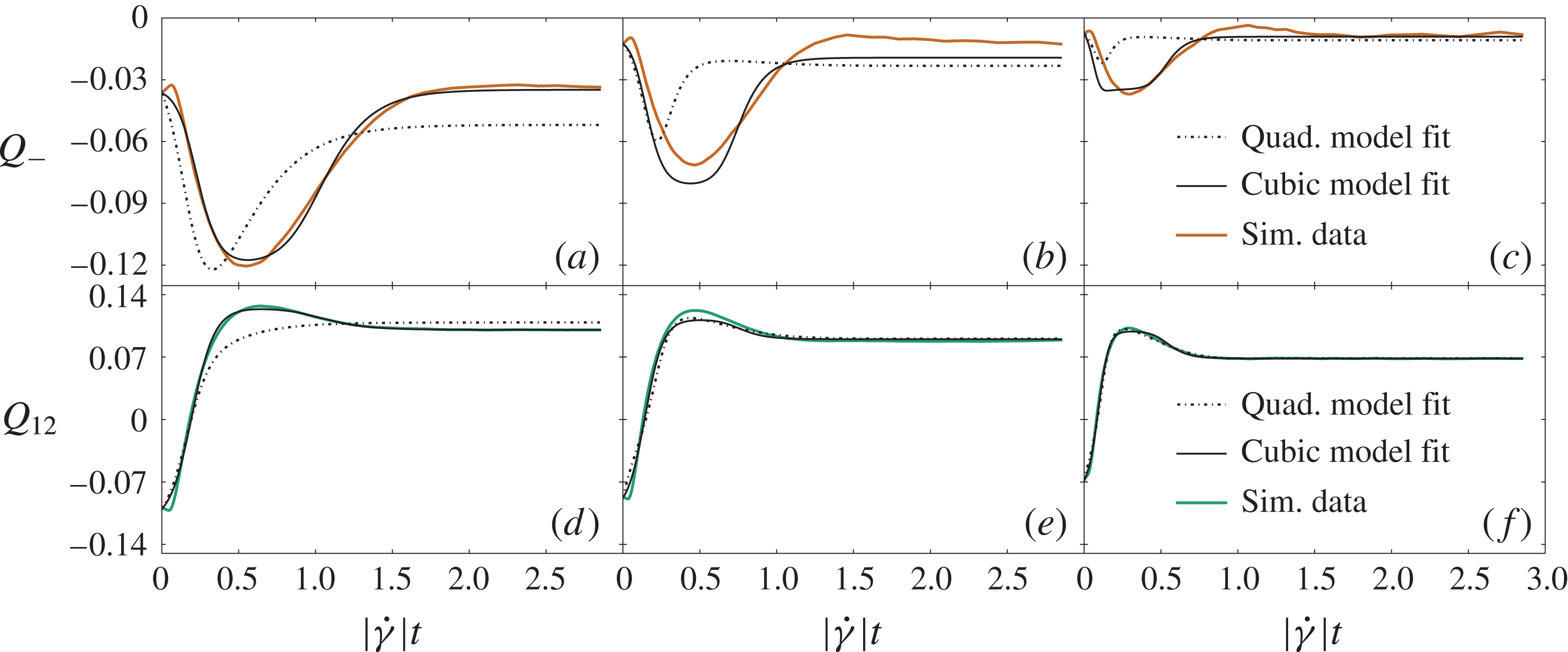
Fits of the quadratic model described by (6.2) and the cubic model described by (6.3) to the two-dimensional fabrics data against post-reversal strain, for both components
 $Q_{-}$
(a–c) and
 $Q_{12}$
(d–f), and for three area fractions
 $\unicode[STIX]{x1D719}=0.65$
(a,d),
 $\unicode[STIX]{x1D719}=0.7$
(b,e) and
 $\unicode[STIX]{x1D719}=0.75$
(c,f).

In figure 10, we show that, while leading to qualitatively correct fits, the quadratic model does not provide a quantitative fit. In particular, the minimum in
 $Q_{-}$
is quite poorly captured, in both position and amplitude, and this discrepancy is accentuated at higher
 $\unicode[STIX]{x1D719}$
. Because of the qualitative similarity between the data in two and three dimensions, we can expect that the three-dimensional fabric dynamics in the shear plane is essentially given by the two-dimensional one, perhaps augmented by a weak coupling to the vorticity direction through a
 $Q_{+}$
term. Indeed, it is hard to imagine a mechanistic interpretation of any quadratic model that would not be expected to work just as well in two dimensions. The fact that (6.2) does not describe even semi-quantitatively the dynamics in two dimensions is telling us that the quadratic model in (5.9) owes its moderate quantitative success to the mathematical freedom of having 11 free parameters rather than to its capturing the underlying physics.
To achieve a near-quantitative fit for the two-dimensional data, we must instead go to cubic order (in the components of
 $\unicode[STIX]{x1D64C}$
) with the model
 $$\begin{eqnarray}\displaystyle \left.\begin{array}{@{}c@{}}P_{-}=a_{-}+c_{-}\operatorname{sgn}(\dot{\unicode[STIX]{x1D6FE}})Q_{12}+e_{-}Q_{12}^{2}+f_{-}Q_{-}^{2},\\ P_{12}=a_{12}+c_{12}\operatorname{sgn}(\dot{\unicode[STIX]{x1D6FE}})Q_{12}+e_{12}Q_{12}^{2}+f_{12}Q_{-}^{2}.\end{array}\right\} & & \displaystyle\end{eqnarray}$$
(This is a cubic model in
 $\unicode[STIX]{x1D64C}$
because
 $P_{-}$
multiplies
 $Q_{-}$
in (6.2).) The data-fitting approach described in the previous section, of using linear least squares on numerically differentiated
 $\unicode[STIX]{x1D64C}$
data to obtain an initial guess for gradient descent, does not work for this cubic model. Indeed, the problem encountered for the three-dimensional quadratic model in the previous section gets even more severe for (6.3), that is, the vast majority of parameter sets entering (6.3) will lead to an unbounded time evolution for
 $\unicode[STIX]{x1D64C}$
, because of the non-confining character of the resulting ODE. This is a commonplace feature of high-order polynomial models with insufficiently constrained parameters. We instead obtain quantitatively superior fits by initiating a gradient descent for a cubic model from the best-fit parameters for the quadratic model of (6.2). This cubic model can fit the data with reasonable accuracy, as shown in figure 10, although the fits to the
 $Q_{-}$
data show room for improvement. More worryingly, signs of overfitting are clearly visible in the
 $Q_{-}$
component. In particular, some short-strain-scale features close to the minimum at intermediate strain values around
 $|\dot{\unicode[STIX]{x1D6FE}}|t\approx 0.5$
appear in the fit.
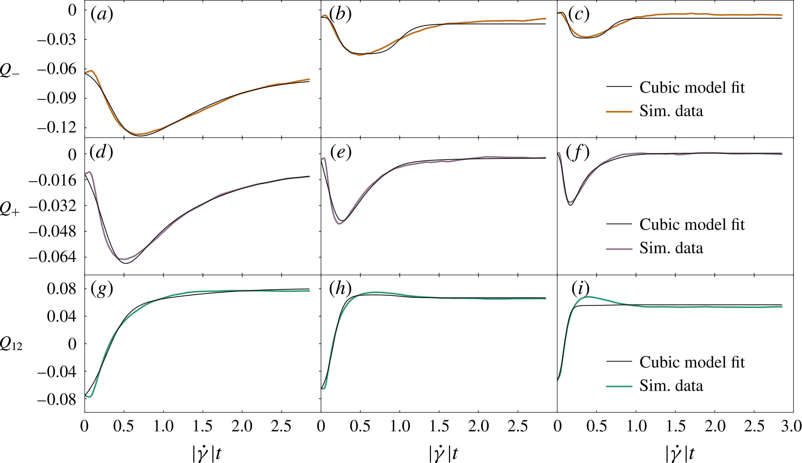
Fits of the cubic model described by (6.4) to three-dimensional simulation data for the components
 $Q_{-}$
(a–c),
 $Q_{+}$
(d–f) and
 $Q_{12}$
(g–i) against post-reversal strain for
 $\unicode[STIX]{x1D719}=0.4$
(a,d,g),
 $\unicode[STIX]{x1D719}=0.5$
(b,e,h) and
 $\unicode[STIX]{x1D719}=0.55$
(c,f,i).

Empirically, we can create a three-dimensional cubic model
 $$\begin{eqnarray}\displaystyle \left.\begin{array}{@{}c@{}}P_{-}=a_{-}+c_{-}\operatorname{sgn}(\dot{\unicode[STIX]{x1D6FE}})Q_{12}+e_{-}Q_{12}^{2}+f_{-}Q_{-}^{2},\\ P_{+}=a_{+}+b_{+}Q_{+}+c_{+}\operatorname{sgn}(\dot{\unicode[STIX]{x1D6FE}})Q_{12}+e_{+}Q_{12}^{2},\\ P_{12}=a_{12}+c_{12}\operatorname{sgn}(\dot{\unicode[STIX]{x1D6FE}})Q_{12}+e_{12}Q_{12}^{2}+f_{12}Q_{-}^{2},\end{array}\right\} & & \displaystyle\end{eqnarray}$$
by supplementing the closed shear-plane dynamics of (6.3) with the vorticity dynamics of (5.9). Although this works quite well (see figure 11), we feel it is unlikely that any mechanical insight can be inferred from this exercise. This is in part due to the large number of parameters involved, and in part due to the smallness of the region in parameter space in which
 $\unicode[STIX]{x1D64C}$
does not blow up when solving the model.
7 Fabric evolution models: limitations
At this stage, we can conclude that any continuum model for
 $\unicode[STIX]{x1D64C}$
in dense non-Brownian suspensions must be of a different and more complicated form than many models for non-Newtonian fluids (Larson Reference Larson2013). Specifically: models linear in
 $\unicode[STIX]{x1D64C}$
are ruled out; models quadratic in
 $\unicode[STIX]{x1D64C}$
fail in two dimensions and are therefore suspect in three; and cubic models generically overfit the data without mechanical insight.
To understand why this approach to finding closed evolution equations for
 $\unicode[STIX]{x1D64C}$
breaks down in dense suspensions, we must revisit our basic assumptions, which are two-fold. Firstly, we assumed in effect that at any instant
 $\unicode[STIX]{x1D64C}$
is an adequate representation of the full probability density of near-contacts
 $P(\boldsymbol{p})$
, that is,
 $P(\boldsymbol{p})$
is well approximated by its second-order spherical harmonic expansion (3.1). In a second and closely related assumption, we postulated that
 $\unicode[STIX]{x1D64C}$
contains enough microstructural information to obtain
 $\dot{\unicode[STIX]{x1D64C}}$
for any given instantaneous strain rate
 $\unicode[STIX]{x1D646}$
, without information from higher moments of
 $P(\boldsymbol{p})$
or even more generally from the entire pair correlation function
 $g(\boldsymbol{r})$
(which includes radial as well as orientational information). Put differently, we can find a closure in
 $\unicode[STIX]{x1D64C}$
that approximates how the higher moments of
 ${\dot{P}}(\boldsymbol{p})$
(higher spherical harmonics) contribute to
 $\dot{\unicode[STIX]{x1D64C}}$
. In principle, the second assumption does not require the first one, but it seems unlikely a priori that
 $\unicode[STIX]{x1D64C}$
determines higher-order spherical harmonic contributions to
 $P(\boldsymbol{p})$
when these are larger than the contribution of
 $\unicode[STIX]{x1D64C}$
itself.
We show in this section that both these assumptions fail for at least parts of the shear reversal. We first assess the adequacy of
 $\unicode[STIX]{x1D64C}$
as a description of the suspension microstructure. In order to compare
 $P(\boldsymbol{p})$
to its successive low-order approximations in terms of spherical harmonics – among which only those of even order contribute – let us recall that the second-order approximation is given by (3.1) and the fourth-order one is (Kanatani Reference Kanatani1984)
 $$\begin{eqnarray}\displaystyle P(\boldsymbol{p})\approx \frac{1}{4\unicode[STIX]{x03C0}}\left(1+\frac{15}{2}\unicode[STIX]{x1D64C}\boldsymbol{ : }\boldsymbol{p}\boldsymbol{p}+\frac{315}{8}\unicode[STIX]{x1D63E}\boldsymbol{ :: }\boldsymbol{p}\boldsymbol{p}\boldsymbol{p}\boldsymbol{p}\right), & & \displaystyle\end{eqnarray}$$
with a fourth-rank structure tensor
 $\unicode[STIX]{x1D63E}$
with components
 $$\begin{eqnarray}\displaystyle C_{ijkl}=\langle p_{i}p_{j}p_{k}p_{l}\rangle -{\textstyle \frac{1}{7}}H_{ijkl}+{\textstyle \frac{1}{35}}I_{ijkl}, & & \displaystyle\end{eqnarray}$$
where
 $$\begin{eqnarray}\displaystyle H_{ijkl} & = & \displaystyle \langle p_{i}p_{j}\rangle \unicode[STIX]{x1D6FF}_{kl}+\langle p_{i}p_{k}\rangle \unicode[STIX]{x1D6FF}_{jl}+\langle p_{i}p_{l}\rangle \unicode[STIX]{x1D6FF}_{jk}+\unicode[STIX]{x1D6FF}_{ij}\langle p_{k}p_{l}\rangle +\unicode[STIX]{x1D6FF}_{ik}\langle p_{j}p_{l}\rangle +\unicode[STIX]{x1D6FF}_{il}\langle p_{j}p_{k}\rangle ,\end{eqnarray}$$
 $$\begin{eqnarray}\displaystyle I_{ijkl} & = & \displaystyle \unicode[STIX]{x1D6FF}_{ij}\unicode[STIX]{x1D6FF}_{kl}+\unicode[STIX]{x1D6FF}_{ik}\unicode[STIX]{x1D6FF}_{jl}+\unicode[STIX]{x1D6FF}_{il}\unicode[STIX]{x1D6FF}_{jk}.\end{eqnarray}$$
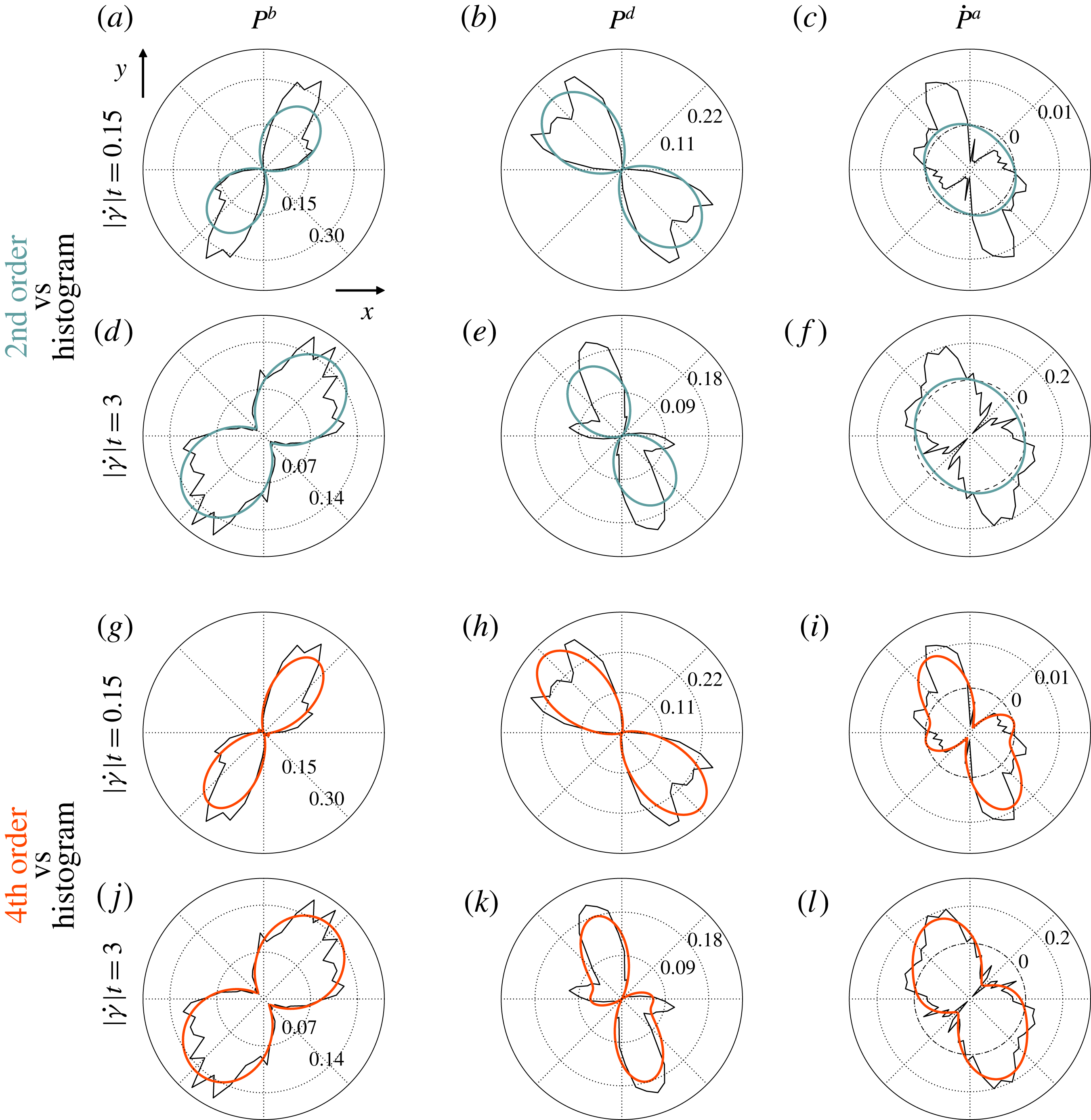
Quantification of the ability of the fabric tensor
 $\unicode[STIX]{x1D64C}$
to capture the major features of the full near-contact orientation distribution function
 $P(\boldsymbol{p})$
during numerical simulations of shear reversal for three volume fractions
 $\unicode[STIX]{x1D719}=0.4$
(a,d,g),
 $\unicode[STIX]{x1D719}=0.5$
(b,e,h) and
 $\unicode[STIX]{x1D719}=0.55$
(c,f,i). (a–c) Polar plots of
 $P(\boldsymbol{p})$
in the shear plane (black line) compared to its second-order spherical harmonic approximation ((3.1), blue line), for the two strain values after reversal indicated on top of each column for each
 $\unicode[STIX]{x1D719}$
. (d–f) Polar plots of the same
 $P(\boldsymbol{p})$
data, compared to its fourth-order spherical harmonic approximation ((7.1), yellow line). (g–i) Largest eigenvalues
 $\unicode[STIX]{x1D6EC}_{2}$
and
 $\unicode[STIX]{x1D6EC}_{4}$
of respectively the second-rank
 $(15/2)\unicode[STIX]{x1D64C}$
and the fourth-rank
 $(315/8)\unicode[STIX]{x1D63E}$
(see main text for the definition) associated, respectively, to second-order and fourth-order contributions in the spherical harmonic expansion of
 $P(\boldsymbol{p})$
.

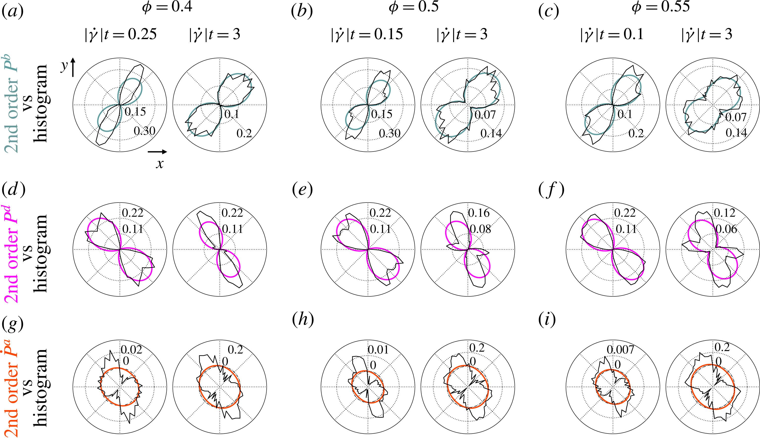
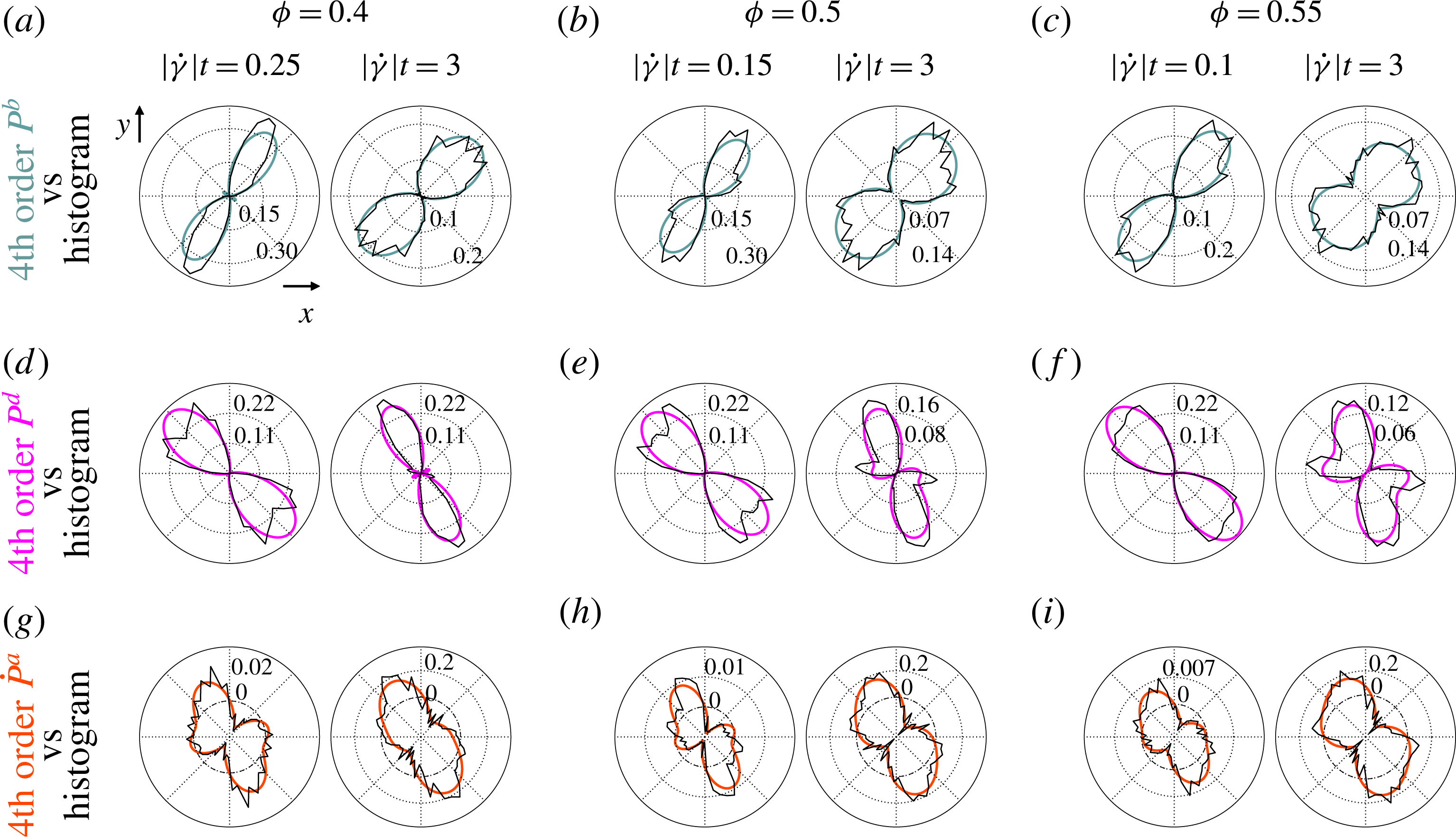
In figure 12(a–f), we evaluate the relative contributions of second- and fourth-rank spherical harmonics to
 $P(\boldsymbol{p})$
for three volume fractions and two representative strains after shear reversal. The first strain,
 $|\dot{\unicode[STIX]{x1D6FE}}|t=0.25$
, 0.15 and 0.1, respectively, for
 $\unicode[STIX]{x1D719}=0.4$
, 0.5 and 0.55, is shortly after reversal and close to the strain at which the principal axes of the microstructure flip over to become the post-reversal compressional and extensional axes. The second strain,
 $|\dot{\unicode[STIX]{x1D6FE}}|t=3$
, corresponds to a microstructure that has reached its post-reversal steady state. In the latter case
 $P(\boldsymbol{p})$
is effectively two-lobed for all three volume fractions, that is, it has two local maxima and two local minima in the shear plane. In this case it is well approximated by its second-order spherical harmonic. However, at smaller strains, during the reconstruction of the contact network after reversal,
 $P(\boldsymbol{p})$
has a distinctive four-lobed structure (that is, four local maxima), which can only be captured by the fourth-order spherical harmonic. For all three volume fractions, at short strains (left column for each volume fraction in figure 12), the second-order approximation is failing to capture the amplitude of the anisotropic features of
 $P(\boldsymbol{p})$
, but even worse it does not even pick the major lobes’ direction.
We can quantify further the four-lobed nature of
 $P(\boldsymbol{p})$
by comparing the largest eigenvalues
 $\unicode[STIX]{x1D6EC}_{2}$
and
 $\unicode[STIX]{x1D6EC}_{4}$
of
 ${\textstyle \frac{15}{2}}\unicode[STIX]{x1D64C}$
and
 ${\textstyle \frac{315}{8}}\unicode[STIX]{x1D63E}$
, respectively (see Qi (Reference Qi2006) for a reference on the eigenvalues of fully symmetric high-order tensors). The time evolution of these eigenvalues under shear reversal is shown in figure 12(g–i) for the same three volume fractions. Here again this reveals at short post-reversal strains an interval across which
 $\unicode[STIX]{x1D63E}$
plays a bigger role than
 $\unicode[STIX]{x1D64C}$
. Even outside this strain interval,
 $\unicode[STIX]{x1D6EC}_{2}$
and
 $\unicode[STIX]{x1D6EC}_{4}$
have the same order of magnitude, including for large strains back to steady state. Importantly though, the breakdown of (3.1) is much more severe in transient flows such as reversal than in steady state.
Nonetheless, an approximation of
 $P(\boldsymbol{p})$
as a function of
 $\unicode[STIX]{x1D64C}$
could be in order provided that the contribution of the fourth-order spherical harmonics could be inferred from the knowledge of the second-order one, that is, provided that there is an accurate closure of
 $\unicode[STIX]{x1D63E}$
in terms of
 $\unicode[STIX]{x1D64C}$
. That the fourth-order spherical harmonics contribute to
 $P(\boldsymbol{p})$
as much as, if not more than, the second-order one makes this possibility unlikely though. The only way to build a fourth-rank tensor out of
 $\unicode[STIX]{x1D64C}$
is by direct product of powers of
 $\unicode[STIX]{x1D64C}$
, hence a closure of
 $\unicode[STIX]{x1D63E}$
must be a weighted sum of terms of the form
 $\unicode[STIX]{x1D64C}^{n}\unicode[STIX]{x1D64C}^{m}$
. Knowing that
 $\unicode[STIX]{x1D64C}$
can be expressed as the sum of dyadic products of its mutually orthogonal eigenvectors
 $\unicode[STIX]{x1D64C}=\sum _{i}\unicode[STIX]{x1D706}_{i}\boldsymbol{e}_{i}\boldsymbol{e}_{i}$
, the contribution to
 $P(\boldsymbol{p})$
of a term
 $\unicode[STIX]{x1D64C}^{n}\unicode[STIX]{x1D64C}^{m}$
in
 $\unicode[STIX]{x1D63E}$
is proportional to (through (7.1))
 $(\unicode[STIX]{x1D64C}^{n}\boldsymbol{ : }\boldsymbol{p}\boldsymbol{p})(\unicode[STIX]{x1D64C}^{m}\boldsymbol{ : }\boldsymbol{p}\boldsymbol{p})$
. In two dimensions (the argument readily extends to the shear plane in three dimensions), if we call
 $\unicode[STIX]{x1D703}$
the angle between
 $\boldsymbol{p}$
and
 $\boldsymbol{e}_{1}$
, then this contribution is
 $\propto (\unicode[STIX]{x1D64C}^{n}\boldsymbol{ : }\boldsymbol{p}\boldsymbol{p})(\unicode[STIX]{x1D64C}^{m}\boldsymbol{ : }\boldsymbol{p}\boldsymbol{p})=\unicode[STIX]{x1D706}_{1}^{m+n}\cos ^{4}\unicode[STIX]{x1D703}+\unicode[STIX]{x1D706}_{2}^{m+n}\sin ^{4}\unicode[STIX]{x1D703}+(\unicode[STIX]{x1D706}_{1}^{m}\unicode[STIX]{x1D706}_{2}^{n}+\unicode[STIX]{x1D706}_{1}^{n}\unicode[STIX]{x1D706}_{2}^{m})\cos ^{2}\unicode[STIX]{x1D703}\sin ^{2}\unicode[STIX]{x1D703}$
. This term is thus in general a four-lobed contribution to
 $P(\boldsymbol{p})$
, but an overly constrained one: the directions of the lobes are the principal axes of
 $\unicode[STIX]{x1D64C}$
, i.e.
 $\boldsymbol{e}_{1}$
and
 $\boldsymbol{e}_{2}$
. Therefore, any closure of
 $\unicode[STIX]{x1D63E}$
in
 $\unicode[STIX]{x1D64C}$
gives a
 $P(\boldsymbol{p})$
with maxima and minima along the directions of the eigenvectors of
 $\unicode[STIX]{x1D64C}$
. Looking back at
 $P(\boldsymbol{p})$
alongside
 $\unicode[STIX]{x1D64C}$
in figure 12(a–f) reveals that at early strains the lobes of
 $P(\boldsymbol{p})$
are not aligned with the principal axes of
 $\unicode[STIX]{x1D64C}$
.
This is a clear indicator that a constitutive model based on a closed ODE for a second-rank fabric evolution under flow cannot capture the physics of near-contact network reconstruction following flow reversal. The strong intrinsic fourth-order component of
 $P(\boldsymbol{p})$
is one of the key outcomes of our analysis. It deems as unphysical closed second-rank fabric evolution models even if they may apparently fit simulation data well, as such a model would base the time evolution on the second-order spherical harmonics, which is subdominant and having incorrect principal axes during a significant part of the time evolution after reversal.
A closer look at the strain derivative
 ${\dot{P}}(\boldsymbol{p})$
confirms this view. As for
 $\unicode[STIX]{x1D64C}$
, we can decompose
 ${\dot{P}}$
into advective, birth and death contributions,
 $$\begin{eqnarray}\displaystyle {\dot{P}}(\boldsymbol{p})={\dot{P}}^{a}(\boldsymbol{p})+r^{b}P^{b}(\boldsymbol{p})-r^{b}P^{d}(\boldsymbol{p}), & & \displaystyle\end{eqnarray}$$
which is derived in appendix C by considering the evolution of the number of near-contacts in a surface element on the unit sphere. Whereas
 $P^{b}(\boldsymbol{p})$
and
 $P^{d}(\boldsymbol{p})$
are positive quantities corresponding to, respectively, the appearance and disappearance of near-contacts,
 ${\dot{P}}^{a}(\boldsymbol{p})$
will in general take positive and negative values in different directions. The three contributions are shown in figure 13 in the shear plane, for
 $\unicode[STIX]{x1D719}=0.5$
and strains
 $|\dot{\unicode[STIX]{x1D6FE}}|t=0.15$
and
 $|\dot{\unicode[STIX]{x1D6FE}}|t=3$
(as in figure 12), alongside their second- and fourth-order spherical harmonics approximations. (The data for
 $\unicode[STIX]{x1D719}=0.4$
and
 $\unicode[STIX]{x1D719}=0.55$
show similar features, and are plotted in appendix D.)
Surprisingly, except for
 $P^{d}(\boldsymbol{p})$
at steady state, none of these distributions show marked four-lobed structures. This is not an inconsistency with the fact that
 $P(\boldsymbol{p})$
is four-lobed during part of the reversal though, as it suffices that the contributions to
 ${\dot{P}}(\boldsymbol{p})$
contribute to accumulate (or deplete) near-contacts in different directions to get a
 $P(\boldsymbol{p})$
with more than two maxima in the shear plane.
Nonetheless, as shown in figure 13(a–f), second-order spherical harmonics approximation fails to capture some essential features of
 $P^{b}(\boldsymbol{p})$
,
 $P^{d}(\boldsymbol{p})$
and
 ${\dot{P}}^{a}(\boldsymbol{p})$
. Moreover, the worst failures occur when these components have large amplitudes relative to the others, that is, at small strains for
 $P^{b}(\boldsymbol{p})$
and at large strains for
 $P^{d}(\boldsymbol{p})$
and
 ${\dot{P}}^{a}(\boldsymbol{p})$
. Some features make these distributions particularly difficult to capture by a second-rank fabric-based approximation. For instance, when
 $P^{d}(\boldsymbol{p})$
shows four lobes, the lobes are consistently found not to be perpendicular to each other. Similarly, even if
 ${\dot{P}}^{a}(\boldsymbol{p})$
is bilobed, the directions associated with minima are not orthogonal to the directions of the maxima, especially at smaller strains. As discussed earlier in this section, these features cannot be captured by analytic functions of
 $\unicode[STIX]{x1D64C}$
. On the other hand, we show in figure 13(g–l) that, for all parameters,
 ${\dot{P}}^{a}(\boldsymbol{p})$
,
 $P^{b}(\boldsymbol{p})$
and
 $P^{d}(\boldsymbol{p})$
are reasonably well approximated by their fourth-order spherical harmonic expansions.
(a–f) Polar plots of simulation data for
 $P^{b}(\boldsymbol{p})$
(a,d,g,j),
 $P^{d}(\boldsymbol{p})$
(b,e,h,k) and
 ${\dot{P}}^{a}(\boldsymbol{p})$
(c,f,i,l), as defined in (7.5), in the shear plane for
 $\unicode[STIX]{x1D719}=0.5$
and for
 $|\dot{\unicode[STIX]{x1D6FE}}|t=0.15$
(a–c) and 3 (d–f), in black lines. These are compared to their second-order spherical harmonic approximations (coloured lines). (g–l) The same
 ${\dot{P}}^{a}(\boldsymbol{p})$
,
 $P^{b}(\boldsymbol{p})$
and
 $P^{d}(\boldsymbol{p})$
data (black lines), compared to their fourth-order spherical harmonic approximations (coloured lines).

Our detailed data for
 $P(\boldsymbol{p})$
, as well as its time derivative, are thus unambiguous: the angular distribution of near-contacts possesses a shear-plane structure only captured by an expansion up to fourth-order in spherical harmonics. As a consequence, the fabric evolution cannot be expressed only in terms of
 $\unicode[STIX]{x1D64C}$
itself, and contains information from the fourth-rank
 $\unicode[STIX]{x1D63E}$
in a way that cannot be approximated by an adequate closure.
8 Discussion
Our detailed interrogation of the numerical data clearly exposes the challenge facing second-rank fabric evolution models, whether considered in themselves or as the basis for a constitutive model for stress evolution under flow. In particular, we use the stringent test of simultaneously modelling the evolution of all components of a
 $3\times 3$
fabric tensor for a suspension under shear reversal. This contrasts our work with previous studies, such as the Sun & Sundaresan (Reference Sun and Sundaresan2011) study, which succeeded in modelling the shear component of a rate-independent granular system in simple shear. As our study has shown, the shear component
 $Q_{12}$
is relatively well behaved and easy to model, as compared to the component
 $Q_{-}$
(see e.g. figures 6 and 7); it is by attempting to model all components simultaneously that the weaknesses of fabric evolution models become apparent. Their failure appears fundamental: the choice of a second-rank fabric tensor to encode the essential features of the microstructural anisotropy is found wanting in shear reversal flows. This is because the orientational distribution of the near-contact interactions (responsible for stress generation)
 $P(\boldsymbol{p})$
, and also its time derivative, strongly depart from the ellipsoidal structures that are the only ones directly described by a second-rank tensor.
We emphasize that this is not a problem of choosing the wrong second-rank tensor to encode the microstructure. Indeed, whereas the small anisotropy of
 $P(\boldsymbol{p})$
at high densities motivates a low-order spherical harmonic expansion in which
 $\unicode[STIX]{x1D64C}$
is the first non-trivial term, other ansätze for
 $P(\boldsymbol{p})$
based on a symmetric second-rank tensor
 $\unicode[STIX]{x1D64F}$
are possible. These include the Bingham distribution ansatz
 $P(\boldsymbol{p})\propto \exp (\unicode[STIX]{x1D64F}\boldsymbol{ : }\boldsymbol{p}\boldsymbol{p})$
(Bingham Reference Bingham1974; Chaubal & Leal Reference Chaubal and Leal1998). In contrast to our (3.1), these ansätze usually contain terms of all orders in the spherical harmonic expansion. Nonetheless, any
 $P(\boldsymbol{p})\propto f(\unicode[STIX]{x1D64F}\boldsymbol{ : }\boldsymbol{p}\boldsymbol{p})$
, with
 $f$
a monotonic function, is still a two-lobed distribution, and in consequence will not adequately describe four-lobed structures in the shear plane, let alone ones in which two pairs of lobes are oriented with non-perpendicular axes. These characteristic four-lobed structures observed for
 $P(\boldsymbol{p})$
and
 ${\dot{P}}(\boldsymbol{p})$
in the shear plane during significant parts of the shear reversal are an intrinsically fourth-order feature in the spherical harmonic expansion. They can best be modelled by introducing the fourth-rank tensor
 $\unicode[STIX]{x1D63E}$
as defined in (7.1) explicitly, and are not adequately captured if
 $\unicode[STIX]{x1D63E}$
is approximated by a closure in terms of
 $\unicode[STIX]{x1D64C}$
.
Given that closure of the hierarchy of tensors appearing in the spherical harmonic expansion of
 $P(\boldsymbol{p})$
cannot be achieved at the
 $\unicode[STIX]{x1D64C}$
level, one could be tempted to develop instead evolution models directly for
 $P(\boldsymbol{p})$
, or even for the entire pair correlation function
 $g(\boldsymbol{r})$
(Nazockdast & Morris Reference Nazockdast and Morris2012, Reference Nazockdast and Morris2013). However, these approaches also require closures (three-point and higher correlations need to be expressed in terms of the two-point one), which might be hard to establish in the absence of powerful results like those of Hand (Reference Hand1962) that strongly limit the number of possibilities.
On the other hand, we showed that
 $P(\boldsymbol{p})$
and its time derivative
 ${\dot{P}}(\boldsymbol{p})$
were both reasonably well approximated by their fourth-order spherical harmonic expansion. This suggests the possibility of developing accurate closed evolution equations for
 $\unicode[STIX]{x1D64C}$
and
 $\unicode[STIX]{x1D63E}$
, that is, closing the hierarchy at the fourth-rank
 $\unicode[STIX]{x1D63E}$
level, effectively expressing the residual higher-order spherical harmonics in terms of
 $\unicode[STIX]{x1D64C}$
and
 $\unicode[STIX]{x1D63E}$
. One step on this route could be an extension of Hand’s result to the fully symmetric fourth-rank tensor
 $\unicode[STIX]{x1D63E}$
. However, one expects this still to lead to a high-dimensional parameter space.
An alternative to postulating general forms and then fitting a large number of parameters is to base a simplified description on a micromechanical ‘kinetic’ theory, including only the terms suggested by that theory. Indeed, this has been a major element in fabric evolution models so far (Hinch & Leal Reference Hinch and Leal1976; Kuzuu & Doi Reference Kuzuu and Doi1983; Phan-Thien Reference Phan-Thien1995). It is perhaps the best way to avoid the generic blowups that emerged above beyond linear order in
 $\unicode[STIX]{x1D64C}$
(since a judicious kinetic theory will presumably map onto parameters within a stable basin of attraction). Clearly, though, in attempting to capture the orientational distribution of near-contacts, this avenue is subject to the same difficulties as outlined above unless a fourth-rank tensor is introduced.
To follow either of these paths to an improved model, further extensive simulations could prove useful. In particular, in order to gain insight into the dynamical coupling of
 $\unicode[STIX]{x1D63E}$
and
 $\unicode[STIX]{x1D64C}$
tensors, it may be enlightening to simulate a purely extensional flow. The additional symmetry beyond that of the shear reversal flows addressed here allows no possible misalignment of the fabric tensor
 $\unicode[STIX]{x1D64C}$
with the flow tensor
 $\hat{\unicode[STIX]{x1D640}}$
, and any four-lobed structures are restricted to those symmetric about the flow axis. In three dimensions, the reversal of a uniaxial extensional flow is a biaxial extensional flow, with therefore an inequivalent steady state. This complicates matters, but, as we have seen, there is much insight to gain from two-dimensional simulations and by extension from three-dimensional planar extensional flow simulations. In that case forward and backward extensional flows are equivalent with the same steady-state microstructure, up to a rotation. Simulations of such extensional flows are achievable even for infinite extensional strains thanks to specific periodic boundary set-ups (Kraynik & Reinelt Reference Kraynik and Reinelt1992; Seto et al.
Reference Seto, Giusteri and Martiniello2017).
It would also be interesting to generalize our studies of shear reversal to the case of shear rotation, in which the direction of shearing is smoothly or suddenly rotated by an angle of less than
 $180^{\circ }$
. Shear reversal is the extreme case where much of the contact network is destroyed before being re-created with the opposite orientation, and the challenges faced by fabric evolution models are most acute in the middle of this process. Such models might be more successful in flows that nudge the fabric from one orientation to another via modest or continuous changes of flow direction. Since the rate independence of dense suspension flows means that all non-reversing shear flow histories with fixed axes are equivalent, shear flows with a non-trivial flow-axis history are perhaps the closest analogue of time-dependent flows in ordinary viscoelastic materials.
Acknowledgements
We would like to thank M. M. Denn for pointing out the literature related to the Bingham closure. The research leading to these results has received funding from SOFI CDT, Durham University, and the EPSRC (grant ref. EP/L015536/1); and from the European Research Council under the European Union’s Seventh Framework Programme (FP7/2007–2013)/ERC grant agreement number 279365. M.E.C. holds a Royal Society Research Professorship.
Appendix A. Numerical method
A.1 Equation of motion
The equation of motion for
 $N$
spheres without inertia is simply the
 $6N$
-dimensional force/torque balance between hydrodynamic (
 $\boldsymbol{F}_{H}$
) and contact (
 $\boldsymbol{F}_{C}$
) interactions, which depends on the positions
 $\boldsymbol{X}$
and the velocities/angular velocities
 $\boldsymbol{U}$
,
 $$\begin{eqnarray}\displaystyle \mathbf{0}=\boldsymbol{F}_{H}(\boldsymbol{X},\boldsymbol{U})+\boldsymbol{F}_{C}(\boldsymbol{X}). & & \displaystyle\end{eqnarray}$$
Equation (A 1) is solved for the velocities, from which the positions are updated at every time step via a mid-point algorithm.
A.2 Hydrodynamic forces
Decomposing the flow
 $\boldsymbol{v}(\boldsymbol{r})=\unicode[STIX]{x1D74E}\times \boldsymbol{r}+\unicode[STIX]{x1D65A}\boldsymbol{\cdot }\boldsymbol{r}$
into rotational
 $\unicode[STIX]{x1D74E}=(0,0,-\dot{\unicode[STIX]{x1D6FE}}/2)$
and extensional
 $\unicode[STIX]{x1D65A}_{12}=\unicode[STIX]{x1D65A}_{21}=\dot{\unicode[STIX]{x1D6FE}}/2$
parts, the lubrication force and torque vector takes the form
 $$\begin{eqnarray}\displaystyle \boldsymbol{F}_{H}(\boldsymbol{X},\boldsymbol{U})=-\unicode[STIX]{x1D64D}_{FU}(\boldsymbol{X})\boldsymbol{\cdot }(\boldsymbol{U}-\boldsymbol{U}^{flow})+\unicode[STIX]{x1D64D}_{FE}(\boldsymbol{X})\boldsymbol{ : }\unicode[STIX]{x1D640}, & & \displaystyle\end{eqnarray}$$
with
 $\boldsymbol{U}^{flow}=(\boldsymbol{v}(\boldsymbol{X}_{1}),\ldots ,\boldsymbol{v}(\boldsymbol{X}_{N}),\unicode[STIX]{x1D74E}(\boldsymbol{X}_{1}),\ldots ,\unicode[STIX]{x1D74E}(\boldsymbol{X}_{N}))$
and
 $\unicode[STIX]{x1D640}=(\unicode[STIX]{x1D65A}(\boldsymbol{X}_{1}),\ldots ,\unicode[STIX]{x1D65A}(\boldsymbol{X}_{N}))$
. The position-dependent resistance second-rank tensor
 $\unicode[STIX]{x1D64D}_{FU}$
and third-rank
 $\unicode[STIX]{x1D64D}_{FE}$
include the so-called ‘squeeze’, ‘shear’ and ‘pump’ modes of lubrication (Ball & Melrose Reference Ball and Melrose1997). The occurrence of contacts between particles in actual suspensions (due to surface roughness, finite-slip boundary conditions, or other factors) is mimicked by a regularization of the resistance divergence at vanishing interparticle gap
 $h_{ij}=2(r_{ij}-a_{i}-a_{j})/(a_{i}+a_{j})$
: the ‘squeeze’ mode is
 $\propto 1/(h+\unicode[STIX]{x1D6FF})$
, and the ‘shear’ and ‘pump’ modes are
 $\propto \log (h+\unicode[STIX]{x1D6FF})$
(Mari et al.
Reference Mari, Seto, Morris and Denn2014), with
 $\unicode[STIX]{x1D6FF}=10^{-3}$
.
A.3 Contact forces
Contacts are modelled by a pair of linear springs and dashpots consisting of both normal and tangential components, a simple model commonly used in granular physics (Cundall & Strack Reference Cundall and Strack1979). The normal and tangential components of the force (respectively,
 $\boldsymbol{f}_{C,nor}^{(i,j)}$
and
 $\boldsymbol{f}_{C,tan}^{(i,j)}$
) and the torque
 $\unicode[STIX]{x1D749}_{C}^{(i,j)}$
applied on a particle
 $i$
in contact with particle
 $j$
(i.e.
 $h_{ij}<0$
) are obtained as
 $$\begin{eqnarray}\displaystyle \left.\begin{array}{@{}c@{}}\boldsymbol{f}_{C,nor}^{(i,j)}=k_{n}h_{ij}\boldsymbol{n}_{ij}+\unicode[STIX]{x1D6FE}_{n}\boldsymbol{u}_{n}^{(i,j)},\\ \boldsymbol{f}_{C,tan}^{(i,j)}=k_{t}\unicode[STIX]{x1D743}^{(i,j)},\\ \unicode[STIX]{x1D749}_{C}^{(i,j)}=a_{i}\boldsymbol{n}_{ij}\times \boldsymbol{f}_{C,tan}^{(i,j)},\end{array}\right\} & & \displaystyle\end{eqnarray}$$
and fulfil Coulomb’s friction law
 $|\boldsymbol{f}_{C,tan}^{(i,j)}|\leqslant \unicode[STIX]{x1D707}|\boldsymbol{f}_{C,nor}^{(i,j)}|$
with a friction coefficient
 $\unicode[STIX]{x1D707}$
. In the above expressions,
 $k_{n}$
and
 $k_{t}$
are the normal and tangential spring constants, respectively, and
 $\unicode[STIX]{x1D6FE}_{n}$
is the damping constant. The normal velocity is
 $\boldsymbol{u}_{n}^{(i,j)}\equiv \boldsymbol{n}_{ij}\boldsymbol{n}_{ij}\boldsymbol{\cdot }(\boldsymbol{V}^{(j)}-\boldsymbol{V}^{(i)})$
, with
 $\boldsymbol{V}$
the particle’s translational velocity. The quantity
 $\unicode[STIX]{x1D743}^{(i,j)}$
is the tangential spring stretch, whose computation follows an algorithm described by Luding (Reference Luding2008) and is designed to enforce Coulomb’s friction law at any time. At the time
 $t_{0}$
at which the contact
 $(i,j)$
is created, we set an unstretched tangential spring
 $\unicode[STIX]{x1D743}^{(i,j)}(t_{0})=\mathbf{0}$
. At any later time step
 $t$
in the simulation, the tangential stretch
 $\unicode[STIX]{x1D743}^{(i,j)}(t)$
is incremented according to the value of a ‘test’ force
 $\boldsymbol{f}_{C,tan}^{\prime (i,j)}(t+\text{d}t)=k_{t}\unicode[STIX]{x1D743}^{\prime (i,j)}(t+\text{d}t)$
, with
 $\unicode[STIX]{x1D743}^{\prime (i,j)}(t+\text{d}t)=\unicode[STIX]{x1D743}^{(i,j)}(t)+\boldsymbol{u}_{t}^{(i,j)}(t)\,\text{d}t$
. In this last expression we use the tangential contact velocity
 $\boldsymbol{u}_{t}^{(i,j)}\equiv (\unicode[STIX]{x1D644}-\boldsymbol{n}_{ij}\boldsymbol{n}_{ij})\boldsymbol{\cdot }[\boldsymbol{V}^{(j)}-\boldsymbol{V}^{(i)}-(a_{i}\unicode[STIX]{x1D734}^{(i)}+a_{j}\unicode[STIX]{x1D734}^{(j)})\times \boldsymbol{n}_{ij}]$
, with
 $\unicode[STIX]{x1D734}$
the particle’s rotational velocity. If
 $|\boldsymbol{f}_{C,tan}^{\prime (i,j)}(t+\text{d}t)|\leqslant \unicode[STIX]{x1D707}|\boldsymbol{f}_{C,nor}^{(i,j)}(t+\text{d}t)|$
, the contact is in a static friction state and we update the spring stretch and force as
 $$\begin{eqnarray}\displaystyle \left.\begin{array}{@{}c@{}}\unicode[STIX]{x1D743}^{(i,j)}(t+\text{d}t)=\unicode[STIX]{x1D743}^{\prime (i,j)}(t+\text{d}t),\\ \boldsymbol{f}_{C,tan}^{(i,j)}(t+\text{d}t)=\boldsymbol{f}_{C,tan}^{\prime (i,j)}(t+\text{d}t).\end{array}\right\} & & \displaystyle\end{eqnarray}$$
However, if
 $|\boldsymbol{f}_{C,tan}^{\prime (i,j)}(t+\text{d}t)|>\unicode[STIX]{x1D707}|\boldsymbol{f}_{C,nor}^{(i,j)}(t+\text{d}t)|$
, the contact is in a sliding state and the spring and force are updated as
 $$\begin{eqnarray}\displaystyle \left.\begin{array}{@{}c@{}}\displaystyle \unicode[STIX]{x1D743}^{(i,j)}(t+\text{d}t)=\frac{\unicode[STIX]{x1D707}}{k_{t}}|\boldsymbol{f}_{C,nor}^{(i,j)}(t+\text{d}t)|\boldsymbol{t}^{(i,j)},\\ \boldsymbol{f}_{C,tan}^{(i,j)}(t+\text{d}t)=k_{t}\unicode[STIX]{x1D743}^{(i,j)}(t+\text{d}t),\end{array}\right\} & & \displaystyle\end{eqnarray}$$
where the direction
 $\boldsymbol{t}^{(i,j)}$
is the same as the one for the test force, i.e.
 $\boldsymbol{t}^{(i,j)}\equiv \boldsymbol{f}_{C,tan}^{\prime (i,j)}(t+\text{d}t)/|\boldsymbol{f}_{C,tan}^{\prime (i,j)}(t+\text{d}t)|$
. In this case, Coulomb’s friction law is saturated, as
 $|\boldsymbol{f}_{C,tan}^{(i,j)}(t+\text{d}t)|=\unicode[STIX]{x1D707}|\boldsymbol{f}_{C,nor}^{(i,j)}(t+\text{d}t)|$
. Note that the static and sliding friction coefficients take the same value
 $\unicode[STIX]{x1D707}$
.
In order to stay as close as possible to a hard-sphere behaviour, the spring stiffnesses are taken such that the largest particle overlaps never exceed 2 % of the particles’ radii during the simulation. By doubling this value, we checked that the shear reversal dynamics is sensitive to the value of the allowed overlap up to a strain of around 1 % after reversal, and is independent of it for later strains.
A.4 Stresses
The bulk stress in the suspension can be decomposed into hydrodynamic and contact contributions. The hydrodynamic stresslets acting on the particles are given by (Batchelor Reference Batchelor1970; Brady & Bossis Reference Brady and Bossis1988)
 $$\begin{eqnarray}\displaystyle \boldsymbol{S}_{H}=-\unicode[STIX]{x1D64D}_{SU}(\boldsymbol{X})\boldsymbol{\cdot }(\boldsymbol{U}-\boldsymbol{U}^{flow})+\unicode[STIX]{x1D64D}_{FE}(\boldsymbol{X})\boldsymbol{ : }\unicode[STIX]{x1D640}, & & \displaystyle\end{eqnarray}$$
where
 $\boldsymbol{S}_{H}=(\boldsymbol{S}_{H}^{(1)},\ldots ,\boldsymbol{S}_{H}^{(N)})$
, and the matrices
 $\unicode[STIX]{x1D64D}_{SU}(\boldsymbol{X})$
and
 $\unicode[STIX]{x1D64D}_{FE}(\boldsymbol{X})$
contain leading terms of the lubrication resistances (Jeffrey & Onishi Reference Jeffrey and Onishi1984; Jeffrey Reference Jeffrey1992) in a manner consistent with the hydrodynamic forces considered in (A 2) (Mari et al.
Reference Mari, Seto, Morris and Denn2014). The stress due to the contact force between particles
 $i$
and
 $j$
is computed as
 $$\begin{eqnarray}\displaystyle \boldsymbol{S}_{C}^{(i,j)}=(\boldsymbol{X}_{j}-\boldsymbol{X}_{i})\boldsymbol{F}_{C}^{(i,j)}. & & \displaystyle\end{eqnarray}$$
Hence the total bulk stress (in which the isotropic part of the fluid pressure is omitted) is
 $$\begin{eqnarray}\displaystyle \unicode[STIX]{x1D72E}\equiv 2\unicode[STIX]{x1D702}_{0}\boldsymbol{E}+\frac{1}{V}\left(\mathop{\sum }_{i}\boldsymbol{S}_{H}^{(i)}+\mathop{\sum }_{i>j}\boldsymbol{S}_{C}^{(i,j)}\right)\!, & & \displaystyle\end{eqnarray}$$
where
 $V$
is the volume of the simulation box.
Appendix B. Componentwise Hand equation for simple shear flow
B.1 In three dimensions
Recall (3.3) and the invariants
 $\hat{I} _{1}$
–
 $\hat{I} _{10}$
. Some of these invariants are trivial in our case. The tensors
 $\unicode[STIX]{x1D64C}$
(by definition) and
 $\hat{\unicode[STIX]{x1D640}}$
(due to incompressibility) are traceless, i.e.
 $\hat{I} _{1}=\hat{I} _{4}=0$
. Moreover, past the instant of shear reversal at
 $\unicode[STIX]{x1D6FE}=0$
,
 $\hat{\unicode[STIX]{x1D640}}$
and thus its powers are constant, which means that
 $\hat{I} _{5}$
and
 $\hat{I} _{6}$
can be absorbed into constant coefficients. We also note that in our case of simple shear flow
 $\boldsymbol{v}=(\dot{\unicode[STIX]{x1D6FE}}y,0,0)$
we have
 $$\begin{eqnarray}\displaystyle \hat{\unicode[STIX]{x1D640}}^{2}\boldsymbol{\cdot }\unicode[STIX]{x1D64C}+\unicode[STIX]{x1D64C}\boldsymbol{\cdot }\hat{\unicode[STIX]{x1D640}}^{2} & = & \displaystyle {\textstyle \frac{1}{2}}\unicode[STIX]{x1D64C}+2\hat{I} _{9}(\unicode[STIX]{x1D644}-4\hat{\unicode[STIX]{x1D640}}^{2}),\end{eqnarray}$$
 $$\begin{eqnarray}\displaystyle \hat{\unicode[STIX]{x1D640}}^{2}\boldsymbol{\cdot }\unicode[STIX]{x1D64C}^{2}+\unicode[STIX]{x1D64C}^{2}\boldsymbol{\cdot }\hat{\unicode[STIX]{x1D640}}^{2} & = & \displaystyle {\textstyle \frac{1}{2}}\unicode[STIX]{x1D64C}^{2}-8\hat{I} _{9}^{2}(\unicode[STIX]{x1D644}-4\hat{\unicode[STIX]{x1D640}}^{2}),\end{eqnarray}$$
so the parameters
 $\unicode[STIX]{x1D6FC}_{7}$
and
 $\unicode[STIX]{x1D6FC}_{8}$
can be set to zero without any loss of generality.
In addition,
 $Q_{13}$
and
 $Q_{23}$
vanish due to the symmetry with respect to the shear plane. In consequence,
 $\unicode[STIX]{x1D64C}$
has only three independent components,
 $Q_{\pm }:=Q_{11}\pm Q_{22}$
and
 $Q_{12}$
. The Hand equation (3.2) for these three components then yields
 $$\begin{eqnarray}\displaystyle \dot{Q}_{-} & = & \displaystyle [\unicode[STIX]{x1D6FC}_{1}+\unicode[STIX]{x1D6FC}_{3}Q_{+}]\operatorname{sgn}(\dot{\unicode[STIX]{x1D6FE}})Q_{-}+2Q_{12},\end{eqnarray}$$
 $$\begin{eqnarray}\displaystyle \dot{Q}_{+} & = & \displaystyle {\textstyle \frac{1}{6}}\unicode[STIX]{x1D6FC}_{4}\operatorname{sgn}(\dot{\unicode[STIX]{x1D6FE}})+\unicode[STIX]{x1D6FC}_{1}\operatorname{sgn}(\dot{\unicode[STIX]{x1D6FE}})Q_{+}+{\textstyle \frac{2}{3}}\unicode[STIX]{x1D6FC}_{5}Q_{12}\nonumber\\ \displaystyle & & \displaystyle +\,\unicode[STIX]{x1D6FC}_{3}\operatorname{sgn}(\dot{\unicode[STIX]{x1D6FE}})\left({\textstyle \frac{1}{6}}Q_{-}^{2}-{\textstyle \frac{1}{2}}Q_{+}^{2}+{\textstyle \frac{2}{3}}Q_{12}^{2}\right)+{\textstyle \frac{2}{3}}\unicode[STIX]{x1D6FC}_{6}Q_{+}Q_{12},\end{eqnarray}$$
 $$\begin{eqnarray}\displaystyle \dot{Q}_{12} & = & \displaystyle {\textstyle \frac{1}{2}}\unicode[STIX]{x1D6FC}_{2}-{\textstyle \frac{1}{2}}Q_{-}+{\textstyle \frac{1}{2}}\unicode[STIX]{x1D6FC}_{5}Q_{+}+\unicode[STIX]{x1D6FC}_{1}\operatorname{sgn}(\dot{\unicode[STIX]{x1D6FE}})Q_{12}\nonumber\\ \displaystyle & & \displaystyle +\,\unicode[STIX]{x1D6FC}_{6}\left({\textstyle \frac{1}{4}}Q_{-}^{2}+{\textstyle \frac{1}{4}}Q_{+}^{2}+Q_{12}^{2}\right)+\unicode[STIX]{x1D6FC}_{3}\operatorname{sgn}(\dot{\unicode[STIX]{x1D6FE}})Q_{+}Q_{12}.\end{eqnarray}$$
Furthermore, in our flow geometry,
 $$\begin{eqnarray}\displaystyle \hat{I} _{2} & = & \displaystyle {\textstyle \frac{1}{2}}Q_{-}^{2}+{\textstyle \frac{3}{2}}Q_{+}^{2}+2Q_{12}^{2},\end{eqnarray}$$
 $$\begin{eqnarray}\displaystyle \hat{I} _{3} & = & \displaystyle {\textstyle \frac{3}{4}}Q_{-}^{2}Q_{+}-{\textstyle \frac{3}{4}}Q_{+}^{3}+3Q_{+}Q_{12}^{2},\end{eqnarray}$$
 $$\begin{eqnarray}\displaystyle \hat{I} _{7} & = & \displaystyle \operatorname{sgn}(\dot{\unicode[STIX]{x1D6FE}})Q_{12},\end{eqnarray}$$
 $$\begin{eqnarray}\displaystyle \hat{I} _{8} & = & \displaystyle \operatorname{sgn}(\dot{\unicode[STIX]{x1D6FE}})Q_{+}Q_{12},\end{eqnarray}$$
 $$\begin{eqnarray}\displaystyle \hat{I} _{9} & = & \displaystyle {\textstyle \frac{1}{4}}Q_{+},\end{eqnarray}$$
 $$\begin{eqnarray}\displaystyle \hat{I} _{10} & = & \displaystyle {\textstyle \frac{1}{8}}Q_{-}^{2}+{\textstyle \frac{1}{8}}Q_{+}^{2}+{\textstyle \frac{1}{2}}Q_{12}^{2}.\end{eqnarray}$$
Since
 $\operatorname{sgn}(\dot{\unicode[STIX]{x1D6FE}})Q_{12}=\hat{I} _{7}$
,
 $Q_{+}=4\hat{I} _{9}$
and
 $Q_{-}^{2}=8\hat{I} _{10}-\hat{I} _{7}^{2}-16\hat{I} _{9}^{2}$
, we see that
 $\hat{I} _{2}$
,
 $\hat{I} _{3}$
and
 $\hat{I} _{8}$
are polynomials in
 $\hat{I} _{7}$
,
 $\hat{I} _{9}$
and
 $\hat{I} _{10}$
, and that an analytic function in the invariants is really an analytic function in
 $\operatorname{sgn}(\dot{\unicode[STIX]{x1D6FE}})Q_{12}$
,
 $Q_{+}$
and
 $Q_{-}^{2}$
. It is thus clear that equations (4.2) hold true.
To show that the Hand equation (3.2) does not constrain
 $\dot{Q}_{-}$
,
 $\dot{Q}_{+}$
and
 $\dot{Q}_{12}$
any further than equations (4.2), consider (3.2) after enforcing tracelessness and proportionality to
 $\dot{\unicode[STIX]{x1D6FE}}$
:
 $$\begin{eqnarray}\displaystyle \operatorname{sgn}(\dot{\unicode[STIX]{x1D6FE}})\dot{\unicode[STIX]{x1D64C}} & = & \displaystyle \hat{\unicode[STIX]{x1D652}}\boldsymbol{\cdot }\unicode[STIX]{x1D64C}-\unicode[STIX]{x1D64C}\boldsymbol{\cdot }\hat{\unicode[STIX]{x1D652}}+\unicode[STIX]{x1D6FD}_{1}\unicode[STIX]{x1D64C}+2(\unicode[STIX]{x1D6FD}_{2}-\unicode[STIX]{x1D6FD}_{1}\hat{I} _{7})\hat{\unicode[STIX]{x1D640}}\nonumber\\ \displaystyle & & \displaystyle +\,6(\unicode[STIX]{x1D6FD}_{4}-4\unicode[STIX]{x1D6FD}_{1}\hat{I} _{9})\hat{\unicode[STIX]{x1D640}}^{2}-2(\unicode[STIX]{x1D6FD}_{4}-4\unicode[STIX]{x1D6FD}_{1}\hat{I} _{9})\hat{I} _{5}\unicode[STIX]{x1D644},\end{eqnarray}$$
corresponding for our flow to the coupled system
 $$\begin{eqnarray}\displaystyle \dot{Q}_{-} & = & \displaystyle \unicode[STIX]{x1D6FD}_{1}\operatorname{sgn}(\dot{\unicode[STIX]{x1D6FE}})Q_{-}+2Q_{12},\end{eqnarray}$$
 $$\begin{eqnarray}\displaystyle \dot{Q}_{+} & = & \displaystyle \unicode[STIX]{x1D6FD}_{4}\operatorname{sgn}(\dot{\unicode[STIX]{x1D6FE}}),\end{eqnarray}$$
 $$\begin{eqnarray}\displaystyle \dot{Q}_{12} & = & \displaystyle \unicode[STIX]{x1D6FD}_{2}-{\textstyle \frac{1}{2}}Q_{-}.\end{eqnarray}$$
Since, as we have established, the only constraint the Hand equation (3.2) imposes on the tensor coefficients
 $\unicode[STIX]{x1D6FD}_{i}$
is that they are are analytic functions (except at
 $\dot{\unicode[STIX]{x1D6FE}}=0$
) of
 $\operatorname{sgn}(\dot{\unicode[STIX]{x1D6FE}})Q_{12}$
,
 $Q_{+}$
and
 $Q_{-}^{2}$
, we may conclude that equations (4.2) are the most general allowed in three dimensions.
B.2 In two dimensions
In two dimensions, the tensorial second-order spherical harmonic expansion (in this case a Fourier series expansion) of a probability density
 $P(\boldsymbol{p})$
for pairs with centre-to-centre orientation
 $\boldsymbol{p}$
is
 $$\begin{eqnarray}\displaystyle P(\boldsymbol{p})\approx \frac{1}{2\unicode[STIX]{x03C0}}(1+4\unicode[STIX]{x1D64C}\boldsymbol{ : }\boldsymbol{p}\boldsymbol{p}), & & \displaystyle\end{eqnarray}$$
where
 $\unicode[STIX]{x1D64C}\equiv \langle \boldsymbol{p}\boldsymbol{p}\rangle -(1/2)\unicode[STIX]{x1D644}$
.
We need to re-derive the Hand equation (3.2) in two dimensions. We start this by noting that the result from frame indifference (Noll Reference Noll1955)
 $$\begin{eqnarray}\displaystyle \frac{\text{d}\unicode[STIX]{x1D64C}}{\text{d}t}=\unicode[STIX]{x1D652}\boldsymbol{\cdot }\unicode[STIX]{x1D64C}-\unicode[STIX]{x1D64C}\boldsymbol{\cdot }\unicode[STIX]{x1D652}+\mathbb{F}(\unicode[STIX]{x1D64C},\unicode[STIX]{x1D640}) & & \displaystyle\end{eqnarray}$$
holds in two dimensions as it does in three. Put differently, the two-dimensional case can be seen as a special case of the three-dimensional case with the axis of the rigid rotation along the vorticity axis.
From (8.13) of Rivlin (Reference Rivlin1955) (after applying (4.7)), any polynomial in symmetric
 $2\times 2$
tensors
 $\unicode[STIX]{x1D63C}$
and
 $\unicode[STIX]{x1D63D}$
can be written in the form
 $$\begin{eqnarray}\displaystyle \unicode[STIX]{x1D711}_{0}\unicode[STIX]{x1D644}+\unicode[STIX]{x1D711}_{1}\unicode[STIX]{x1D63C}+\unicode[STIX]{x1D711}_{2}\unicode[STIX]{x1D63D}, & & \displaystyle\end{eqnarray}$$
where the
 $\unicode[STIX]{x1D711}_{i}$
are polynomials in the invariants (see paragraph in Rivlin (Reference Rivlin1955) below (13.3))
 $\text{Tr}\,\unicode[STIX]{x1D63C}$
,
 $\text{Tr}\,\unicode[STIX]{x1D63D}$
,
 $\text{Tr}\,\unicode[STIX]{x1D63C}^{2}$
,
 $\text{Tr}\,\unicode[STIX]{x1D63D}^{2}$
and
 $\text{Tr}\,\unicode[STIX]{x1D63C}\boldsymbol{\cdot }\unicode[STIX]{x1D63D}$
.
We can therefore write the rate-independent two-dimensional Hand equation for
 $\unicode[STIX]{x1D64C}$
,
 $$\begin{eqnarray}\displaystyle \operatorname{sgn}(\dot{\unicode[STIX]{x1D6FE}})\dot{Q}=\hat{\unicode[STIX]{x1D652}}\boldsymbol{\cdot }\unicode[STIX]{x1D64C}-\unicode[STIX]{x1D64C}\boldsymbol{\cdot }\hat{\unicode[STIX]{x1D652}}+\unicode[STIX]{x1D6FC}_{1}\unicode[STIX]{x1D64C}+\unicode[STIX]{x1D6FC}_{2}\hat{\unicode[STIX]{x1D640}}, & & \displaystyle\end{eqnarray}$$
or in component form,
 $$\begin{eqnarray}\displaystyle \left.\begin{array}{@{}c@{}}\dot{Q}_{-}=\unicode[STIX]{x1D6FC}_{1}\operatorname{sgn}(\dot{\unicode[STIX]{x1D6FE}})Q_{-}+2Q_{12},\\ \dot{Q}_{12}={\textstyle \frac{1}{2}}\unicode[STIX]{x1D6FC}_{2}-{\textstyle \frac{1}{2}}Q_{-}+\unicode[STIX]{x1D6FC}_{1}\operatorname{sgn}(\dot{\unicode[STIX]{x1D6FE}})Q_{12},\end{array}\right\} & & \displaystyle\end{eqnarray}$$
with the
 $\unicode[STIX]{x1D6FC}_{i}$
analytic functions of the invariants
 $\hat{I} _{1}\equiv \text{Tr}(\unicode[STIX]{x1D64C})$
,
 $\hat{I} _{2}\equiv \text{Tr}(\unicode[STIX]{x1D64C}^{2})$
,
 $\hat{I} _{4}\equiv \text{Tr}(\hat{\unicode[STIX]{x1D640}})$
,
 $\hat{I} _{5}\equiv \text{Tr}(\hat{\unicode[STIX]{x1D640}}^{2})$
and
 $\hat{I} _{7}\equiv \text{Tr}(\unicode[STIX]{x1D64C}\boldsymbol{\cdot }\hat{\unicode[STIX]{x1D640}})$
. Here the labelling is chosen so as to be consistent with the three-dimensional case.
For an incompressible shear flow in two dimensions
 $\boldsymbol{v}=(\dot{\unicode[STIX]{x1D6FE}}y,0)$
, the invariants are
 $$\begin{eqnarray}\displaystyle \hat{I} _{1} & = & \displaystyle 0,\end{eqnarray}$$
 $$\begin{eqnarray}\displaystyle \hat{I} _{2} & = & \displaystyle {\textstyle \frac{1}{2}}Q_{-}^{2}+2Q_{12}^{2},\end{eqnarray}$$
 $$\begin{eqnarray}\displaystyle \hat{I} _{4} & = & \displaystyle 0,\end{eqnarray}$$
 $$\begin{eqnarray}\displaystyle \hat{I} _{5} & = & \displaystyle {\textstyle \frac{1}{2}},\end{eqnarray}$$
 $$\begin{eqnarray}\displaystyle \hat{I} _{7} & = & \displaystyle \operatorname{sgn}(\dot{\unicode[STIX]{x1D6FE}})Q_{12}.\end{eqnarray}$$
We see that an analytical function of the invariants is an analytical function of
 $\operatorname{sgn}(\dot{\unicode[STIX]{x1D6FE}})Q_{12}$
and
 $Q_{-}^{2}$
, so that the most general form of the two-dimensional Hand equation for our system is
 $$\begin{eqnarray}\displaystyle \dot{Q}_{-} & = & \displaystyle P_{-}[\operatorname{sgn}(\dot{\unicode[STIX]{x1D6FE}})Q_{12},Q_{-}^{2}]\operatorname{sgn}(\dot{\unicode[STIX]{x1D6FE}})Q_{-}+2Q_{12},\end{eqnarray}$$
 $$\begin{eqnarray}\displaystyle \dot{Q}_{12} & = & \displaystyle P_{12}[\operatorname{sgn}(\dot{\unicode[STIX]{x1D6FE}})Q_{12},Q_{-}^{2}]-{\textstyle \frac{1}{2}}Q_{-},\end{eqnarray}$$
where the
 $P_{ij}$
are analytical functions of their arguments.
Appendix C. Decomposition of the fabric evolution
The near-contact angular distribution at a strain
 $\unicode[STIX]{x1D6FE}$
is defined as
 $$\begin{eqnarray}\displaystyle P_{\unicode[STIX]{x1D6FE}}(\boldsymbol{p})=\frac{1}{N_{\unicode[STIX]{x1D6FE}}}\mathop{\sum }_{i}\unicode[STIX]{x1D6FF}[\boldsymbol{p}-\boldsymbol{p}_{i}(\unicode[STIX]{x1D6FE})]. & & \displaystyle\end{eqnarray}$$
Between any two successive strain steps
 $\unicode[STIX]{x1D6FE}$
and
 $\unicode[STIX]{x1D6FE}+\text{d}\unicode[STIX]{x1D6FE}$
, we can separate the evolution of this distribution into three kinds of events:
(i) a near-contact disappears between
$\unicode[STIX]{x1D6FE}$
and
$\unicode[STIX]{x1D6FE}+\text{d}\unicode[STIX]{x1D6FE}$
(death),(ii) a near-contact appears between
$\unicode[STIX]{x1D6FE}$
and
$\unicode[STIX]{x1D6FE}+\text{d}\unicode[STIX]{x1D6FE}$
(birth),(iii) a near-contact survives between
$\unicode[STIX]{x1D6FE}$
and
$\unicode[STIX]{x1D6FE}+\text{d}\unicode[STIX]{x1D6FE}$
and is just advected.


Hence we can write
 $$\begin{eqnarray}\displaystyle P_{\unicode[STIX]{x1D6FE}+\text{d}\unicode[STIX]{x1D6FE}}(\boldsymbol{p})-P_{\unicode[STIX]{x1D6FE}}(\boldsymbol{p}) & = & \displaystyle \mathop{\sum }_{i\in advected}\frac{1}{N_{\unicode[STIX]{x1D6FE}+\text{d}\unicode[STIX]{x1D6FE}}}\unicode[STIX]{x1D6FF}[\boldsymbol{p}-\boldsymbol{p}_{i}(\unicode[STIX]{x1D6FE}+\text{d}\unicode[STIX]{x1D6FE})]-\frac{1}{N_{\unicode[STIX]{x1D6FE}}}\unicode[STIX]{x1D6FF}[\boldsymbol{p}-\boldsymbol{p}_{i}(\unicode[STIX]{x1D6FE})]\nonumber\\ \displaystyle & & \displaystyle +\,\frac{1}{N_{\unicode[STIX]{x1D6FE}+\text{d}\unicode[STIX]{x1D6FE}}}\mathop{\sum }_{i\in birth}\unicode[STIX]{x1D6FF}[\boldsymbol{p}-\boldsymbol{p}_{i}(\unicode[STIX]{x1D6FE}+\text{d}\unicode[STIX]{x1D6FE})]-\frac{1}{N_{\unicode[STIX]{x1D6FE}}}\mathop{\sum }_{i\in death}\unicode[STIX]{x1D6FF}[\boldsymbol{p}-\boldsymbol{p}_{i}(\unicode[STIX]{x1D6FE})].\quad\end{eqnarray}$$
Now, calling
 $N_{birth}$
and
 $N_{death}$
the number of near-contacts, respectively, being born and dying between
 $\unicode[STIX]{x1D6FE}$
and
 $\unicode[STIX]{x1D6FE}+\text{d}\unicode[STIX]{x1D6FE}$
, we define
 $$\begin{eqnarray}\displaystyle {\dot{P}}^{a}(\boldsymbol{p}) & := & \displaystyle \frac{1}{\text{d}\unicode[STIX]{x1D6FE}}\mathop{\sum }_{i\in advected}\frac{1}{N_{\unicode[STIX]{x1D6FE}+\text{d}\unicode[STIX]{x1D6FE}}}\unicode[STIX]{x1D6FF}[\boldsymbol{p}-\boldsymbol{p}_{i}(\unicode[STIX]{x1D6FE}+\text{d}\unicode[STIX]{x1D6FE})]-\frac{1}{N_{\unicode[STIX]{x1D6FE}}}\unicode[STIX]{x1D6FF}[\boldsymbol{p}-\boldsymbol{p}_{i}(\unicode[STIX]{x1D6FE})],\end{eqnarray}$$
 $$\begin{eqnarray}\displaystyle P^{b}(\boldsymbol{p}) & := & \displaystyle \frac{1}{N_{birth}}\mathop{\sum }_{i\in birth}\unicode[STIX]{x1D6FF}[\boldsymbol{p}-\boldsymbol{p}_{i}(\unicode[STIX]{x1D6FE}+\text{d}\unicode[STIX]{x1D6FE})],\end{eqnarray}$$
 $$\begin{eqnarray}\displaystyle P^{d}(\boldsymbol{p}) & := & \displaystyle \frac{1}{N_{death}}\mathop{\sum }_{i\in death}\unicode[STIX]{x1D6FF}[\boldsymbol{p}-\boldsymbol{p}_{i}(\unicode[STIX]{x1D6FE})],\end{eqnarray}$$
so that
 $$\begin{eqnarray}\displaystyle {\dot{P}}_{\unicode[STIX]{x1D6FE}}(\boldsymbol{p})={\dot{P}}^{a}(\boldsymbol{p})+r^{b}P^{b}(\boldsymbol{p})-r^{d}P^{d}(\boldsymbol{p}), & & \displaystyle\end{eqnarray}$$
which is (7.5) in the main text, with the birth and death rates
 $r^{b}=N_{birth}/(N_{\unicode[STIX]{x1D6FE}+\text{d}\unicode[STIX]{x1D6FE}}\,\text{d}\unicode[STIX]{x1D6FE})$
and
 $r^{d}=N_{death}/(N_{\unicode[STIX]{x1D6FE}}\,\text{d}\unicode[STIX]{x1D6FE})$
.
Taking the traceless second moment of
 ${\dot{P}}^{a}$
,
 $P^{b}$
and
 $P^{d}$
, we can also get a decomposition of the strain derivative of the fabric tensor:
 $$\begin{eqnarray}\displaystyle \dot{\unicode[STIX]{x1D64C}}=\dot{\unicode[STIX]{x1D64C}}^{a}+r^{b}\unicode[STIX]{x1D64C}^{b}(\boldsymbol{p})-\unicode[STIX]{x1D64C}^{d}P^{d}(\boldsymbol{p}), & & \displaystyle\end{eqnarray}$$
which is (5.7) in the main text.
Appendix D. Plots of advective, birth and death components of
${\dot{P}}(\boldsymbol{p})$

Figure 14.

Figure 14 shows polar plots of simulation data for
 $P^{b}(\boldsymbol{p})$
(a–c),
 $P^{d}(\boldsymbol{p})$
(d–f) and
 ${\dot{P}}^{a}(\boldsymbol{p})$
(g–i), as defined in (7.5), in the shear plane (black lines) compared to their second-order spherical harmonic approximations (coloured lines), for
 $\unicode[STIX]{x1D719}=0.4$
(a, d, g),
 $\unicode[STIX]{x1D719}=0.5$
(b,e,h) and
 $\unicode[STIX]{x1D719}=0.55$
(c,f,i), and for the two strain values after reversal indicated on top of each
 $\unicode[STIX]{x1D719}$
column. Figure 15 shows the same data compared to their fourth-order spherical harmonic approximations.
Figure 15.

Appendix E. Tables of fit parameter values
For reference, tables 1–4 list the parameter values for the fits used in this paper. For nonlinear models, we do not expect any particular trend in the dependence on volume fraction of fit parameters, since our fits correspond to finding one local minimum in a high-dimensional energy landscape with many. Even a small quantitative shift of the simulation data can change the energy landscape enough to lead us down a different minimum when applying our fitting methodology. If there was a mechanistic insight in the terms in the model, one would expect a trend in the coefficient values; the absence of such a trend may be a manifestation of a perhaps good but mechanistically accidental fit.