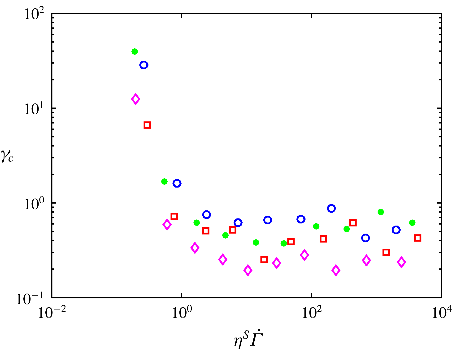
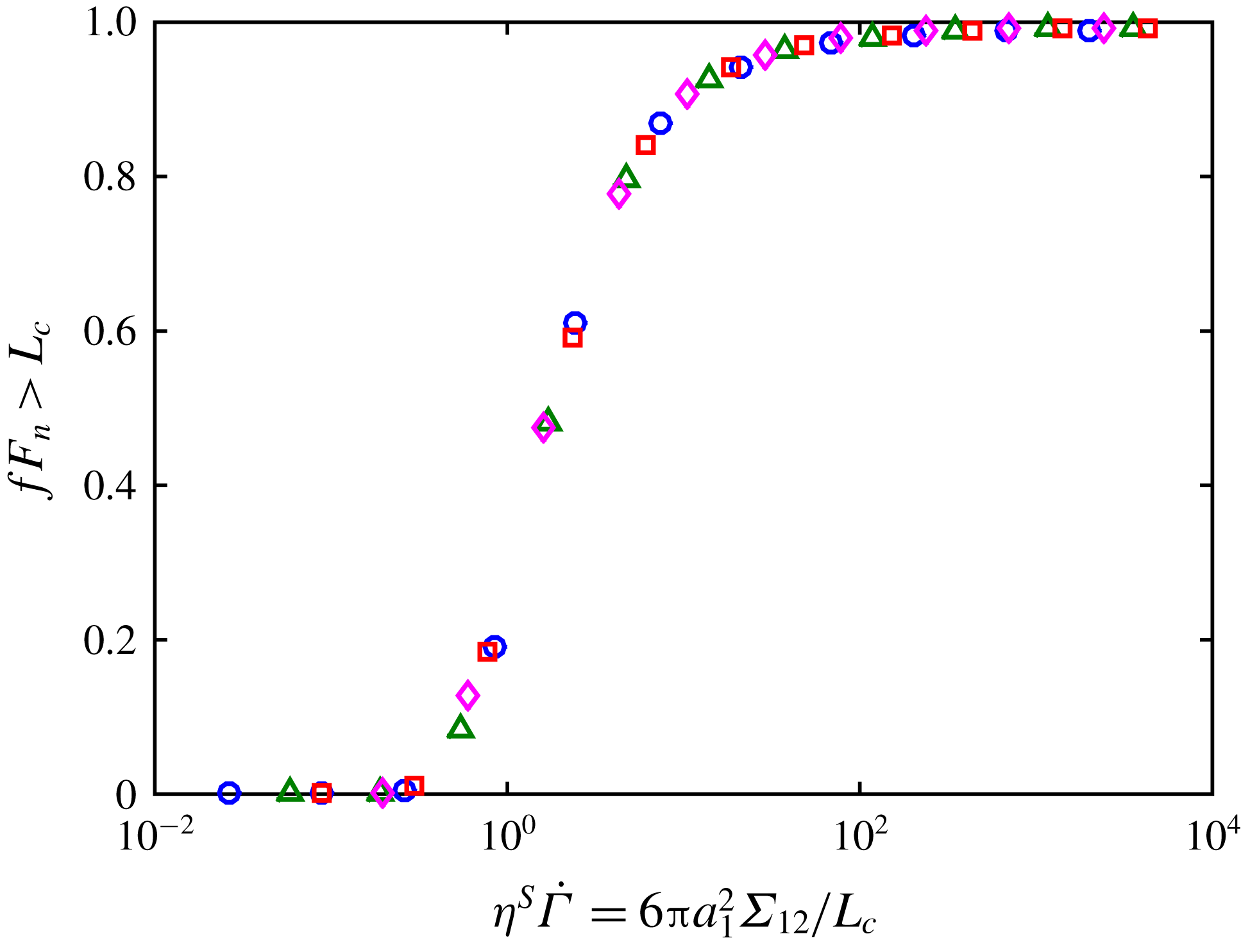
1 Introduction
Suspensions of rigid particles in low Reynolds number flows are ubiquitous in industry (food transport, cosmetic products, civil engineering, etc.) or natural flows (such as mud or lava flows) to mention but a few. This wide occurrence of suspensions has fostered significant research in the past years that has revealed a great complexity in the behaviour of these systems. Concentrated suspensions may present shear-thinning or shear-thickening behaviours, anisotropic normal stresses, irreversibility under oscillating shear and many other complex behaviours. Some of these features come from the possible complexity of the suspensions themselves. For instance, the suspending liquid may be non-Newtonian, particles may have irregular shape, be elongated or faceted, be deformable or polydisperse, they may interact through colloidal forces, Brownian or buoyancy forces may exist, etc. But it is quite fascinating that even very simple ‘model’ suspensions made of non-Brownian, non-colloidal, monodisperse spherical particles dispersed in a Newtonian fluid exhibit non-Newtonian behaviours. Most of these behaviours may be explained by the coupling between flow, contact interactions and microstructure. To mention just a few examples, Pham, Metzger & Butler (Reference Pham, Metzger and Butler2015) showed that irreversible dynamics of non-Brownian neutrally buoyant particles subjected to a periodic shear flow originates in particle solid–solid contacts. Gadala-Maria & Acrivos (Reference Gadala-Maria and Acrivos1980) proposed an explanation for the transient response of the viscosity under shear reversal by the presence of an asymmetric shear-induced microstructure that is broken and rebuilt along the new direction of the flow. Later Blanc, Peters & Lemaire (Reference Blanc, Peters and Lemaire2011) showed that the asymmetry of the microstructure comes from solid contact between particles through the asperities they have at their surface. The involvement of contact forces has also made it possible to explain the discontinuous shear thickening often observed in very concentrated suspensions of non-Brownian spheres (Seto et al.
Reference Seto, Mari, Morris and Denn2013; Mari et al.
Reference Mari, Seto, Morris and Denn2014) by a transition from frictionless to frictional contacts. The effect of solid friction between particles on both normal stress differences and viscosity of concentrated suspensions is also very significant. Numerical simulations of Gallier et al. (Reference Gallier, Lemaire, Peters and Lobry2014) showed that changing the friction coefficient,
 $\unicode[STIX]{x1D707}$
, from 0 to 0.5 for a 0.45 volume fraction suspension leads to an increase of the viscosity by a factor of 1.5 while the first normal stress difference magnitude – which is negative – is divided by almost 2 and the second normal stress is twofold increased. As the particle volume fraction,
 $\unicode[STIX]{x1D719}$
, increases, the contribution of contact forces to the viscosity becomes more and more important compared to the contribution of hydrodynamic forces. For rough frictional particles with
 $\unicode[STIX]{x1D707}=0.5$
, hydrodynamic and contact contributions are almost the same for
 $\unicode[STIX]{x1D719}=0.4$
but, at
 $\unicode[STIX]{x1D719}=0.46$
, the contact contribution is approximately twice the hydrodynamic contribution. So one has to keep in mind that the solid contacts between particles are a key ingredient to explain non-Brownian suspension rheology.
Among non-Newtonian behaviours that still raise questions, shear thinning occupies a special place because it is quite ubiquitous and can be observed in most experimental results on shear rate–shear stress dependence but is rarely discussed. A first attempt to explain shear thinning has been made by Acrivos, Fan & Mauri (Reference Acrivos, Fan and Mauri1994) who showed that the apparent shear thinning that they observed when the viscosity of a suspension of non-Brownian particles is measured in a Couette device is due to a mismatch in the densities of the liquid and of the particles. But whereas this explanation seems compelling in the case of the Couette flow, where the larger and larger resuspension of the denser particles as the shear rate increases should lead to a decrease of the measured apparent viscosity, it cannot explain shear thinning observed in other flow geometries such as for example in torsional parallel-plate flow. Shear thinning, however, has been reported in rotating parallel-plate measurements by several authors (Zarraga, Hill & Leighton Jr Reference Zarraga, Hill and Leighton2000; Dbouk Reference Dbouk2011; Vázquez-Quesada, Tanner & Ellero Reference Vázquez-Quesada, Tanner and Ellero2016). Vázquez-Quesada et al. (Reference Vázquez-Quesada, Tanner and Ellero2016) explains the shear thinning they observed by the shear-thinning behaviour of the suspending liquid (silicon oil) itself. More precisely, the suspending liquid is Newtonian at the macroscopic shear rates involved in the measurement of the viscosity but may be shear thinning in the range of the higher shear rates experienced by the host liquid in the interparticle gap. Later, the authors showed that this mechanism cannot apply for all systems and suggested that variable contact friction between particles may also be responsible for shear thinning (Vazquez-Quesada et al. Reference Vazquez-Quesada, Mahmud, Dai, Ellero and Tanner2017). Recently, Tanner et al. (Reference Tanner, Ness, Mahmud, Dai and Moon2018) proposed a model based on a bootstrap mechanism of friction that introduces shear thinning by assuming that the friction coefficient is a decreasing function of the sliding speed between particles. Here, we explore the same kind of idea and propose to explain shear thinning by a decrease of the friction coefficient between particles as the contact force between them, which is controlled by the suspension shear stress, increases. Prior to describing the contact law between particles, we would like to highlight that particle contacts are enabled by the asperities that are present at particle surface. For perfectly smooth particles, solid contact is prevented by lubrication forces that diverge as the particle separation tends to zero. By contrast, for rough particles, contact between particles is made possible through isolated asperities that maintain finite lubrication forces between particles. In other words, roughness is able to screen lubrication divergence. In such a scenario, only one or a few asperities may be involved in contact, and the macroscopic Amontons–Coulomb law, used to describe contact between macroscopic surfaces and according to which the friction coefficient does not depend on the magnitude of the tangential or normal load, is expected not to hold anymore. Indeed, this macroscopic contact law is usually understood in the frame of theories where a large number of asperities are compressed (Greenwood & Williamson Reference Greenwood and Williamson1966). Instead, in the case of a small number of elastically contacting asperities, the friction coefficient is expected to decrease with load (Archard Reference Archard1957).
In the present paper, we modify the contact model presented in Gallier et al. (Reference Gallier, Lemaire, Peters and Lobry2014) in order to account for a variable friction between particles. The first part is dedicated to the presentation of the numerical method and of the contact model that has been chosen to introduce a load-dependent friction coefficient in the numerical simulations. The second section presents the simulation results and proposes a viscosity model that makes it possible to estimate the influence of any particular friction law on the viscosity without performing new simulations. In the third section, experiments carried out on suspensions of monodisperse polystyrene particles,
 $40~\unicode[STIX]{x03BC}\text{m}$
in diameter, dispersed in a silicone oil for five values of the particle volume fraction are presented. And the last section is devoted to a comparison of the numerical model to the experimental results.
2 Numerical method
2.1 The force coupling method
We use the force coupling method to study the rheology of non-Brownian suspensions made of rigid rough particles in a Newtonian liquid,
 $\unicode[STIX]{x1D702}_{0}$
in viscosity. The main features of the method are recalled in Peters et al. (Reference Peters, Ghigliotti, Gallier, Blanc, Lemaire and Lobry2016) and the interested reader will find more detail in Yeo & Maxey (Reference Yeo and Maxey2010b
). In this method, the motion of the fluid is computed in the whole meshed domain, where the presence of the particles is taken into account using a specified force density that enforces rigid body motion in the particles. Small scale flows between the particles are not resolved by the direct computation, so that the hydrodynamic force and other moments are corrected using theoretical expressions from lubrication approximation. Thus, this method is able to catch both long-range and short-range hydrodynamic interactions. Inertia is neglected in computing both the liquid and the particle motion, and the particle density is matched to that of the liquid. As a consequence, the total force and torque on each particle vanish:
 $$\begin{eqnarray}\displaystyle & \displaystyle \boldsymbol{F}^{h}+\boldsymbol{F}^{c}=0, & \displaystyle\end{eqnarray}$$
 $$\begin{eqnarray}\displaystyle & \displaystyle \boldsymbol{T}^{h}+\boldsymbol{T}^{c}=0, & \displaystyle\end{eqnarray}$$
where the superscript
 $h$
stands for the hydrodynamic moments (both direct computation and lubrication corrections) and
 $c$
for the contact moments. The latter will be described in the following section, and the former are computed as explained in Peters et al. (Reference Peters, Ghigliotti, Gallier, Blanc, Lemaire and Lobry2016). The hydrodynamic force moment (stresslet)
 $\unicode[STIX]{x1D64E}^{h}$
as well as the contact force moment
 $\unicode[STIX]{x1D64E}^{c}$
of each particle are computed too, yielding the effective stress, and then the relative viscosity
 $\unicode[STIX]{x1D702}^{S}$
, which is defined as the ratio of the suspension viscosity to the host liquid viscosity.
The particles are contained in a cubic domain, where the shear rate
 $\dot{\unicode[STIX]{x1D6FE}}$
is imposed. The flow is made periodic in all three dimensions using Lee Edwards conditions. The total solid volume fraction is denoted by
 $\unicode[STIX]{x1D719}$
. We consider a bidisperse collection of spheres, of radius
 $a_{1}$
and
 $a_{2}=1.4a_{1}$
, with the same volume fraction
 $\unicode[STIX]{x1D719}/2$
, in order to avoid crystallisation. The particular value
 $a_{1}/a_{2}=1.4$
that was chosen is widely used in the literature (Seto et al.
Reference Seto, Mari, Morris and Denn2013; Mari et al.
Reference Mari, Seto, Morris and Denn2014; Ness & Sun Reference Ness and Sun2015; Seto, Giusteri & Martiniello Reference Seto, Giusteri and Martiniello2017). We note here that a recent study was published, that explored the influence of bidispersity on the suspension rheology, and compared it to polydisperse system rheology (Pednekar, Chun & Morris Reference Pednekar, Chun and Morris2018). From this study, it is possible to infer that, at least for the volume fraction range that is probed in the present article, the viscosity is nearly the same as for a monodisperse system without crystallisation. The size of the computation cell is
 $L_{x}\times L_{y}\times L_{z}=16a_{1}\times 16a_{1}\times 16a_{1}$
corresponding to approximately 300 particles for a solid volume fraction
 $\unicode[STIX]{x1D719}=0.5$
. The suspension is sheared during a total strain ranging between 40 and 100, depending on the solid volume fraction, in order to obtain correct averaging.
2.2 Contact model
2.2.1 Introduction
Up to now, most simulations of sheared frictional suspensions (Seto et al. Reference Seto, Mari, Morris and Denn2013; Gallier et al. Reference Gallier, Lemaire, Peters and Lobry2014; Mari et al. Reference Mari, Seto, Morris and Denn2014; Peters et al. Reference Peters, Ghigliotti, Gallier, Blanc, Lemaire and Lobry2016) have considered a simple model of frictional contact with a constant static friction coefficient, as defined by the ratio of the largest tangential force that is allowed before sliding motion occurs to the normal force. This simple Amontons–Coulomb model is a simplified description of the contact between macroscopic surfaces for which the real area of contact is far smaller than the apparent macroscopic contact area, meaning that contact occurs between surface asperities (Tabor Reference Tabor1981). Considering a macroscopic contact, it is usually assumed that a statistically large number of asperities are deformed, as in Greenwood & Williamson (Reference Greenwood and Williamson1966). Even though the contact area for each single asperity is not proportional to the corresponding load, the total area is approximately proportional to the total load, leading to a static friction coefficient that does not depend on the load, in agreement with the Amontons–Coulomb law.
Contrarily, when a contact between a single asperity and a smooth surface is considered, the contact law is not linear anymore and a decrease of the friction coefficient with increasing normal load is expected. Many models have been proposed, where the deformation remains elastic at low applied load, and enters a plastic regime as the load is increased (see for example Chang, Etsion & Bogy Reference Chang, Etsion and Bogy1987; Brizmer et al. Reference Brizmer, Zait, Kligerman and Etsion2006b ; Brizmer, Kligerman & Etsion Reference Brizmer, Kligerman and Etsion2007), and some experimental validations have been performed for the contact of a smooth sphere against a flat substrate, leading to a load-dependent static friction coefficient (Ovcharenko, Halperin & Etsion Reference Ovcharenko, Halperin and Etsion2008).
The present paper deals with contacting micro-particles immersed in a host liquid, the whole suspension experiencing a shear flow. This particular problem may be considered quite specific for several reasons. First, the contact forces that are controlled by the sheared suspension bulk stress may be very weak, depending on the shear rate and the volume fraction. As a consequence, contact occurs between a small number of asperities and not between a large distribution of asperities as in Greenwood–Williamson model (see § 2.2.4 for details on the model parameters and the estimation of the number of contacting asperities). Hence a load-dependent friction coefficient is expected, instead of the Amontons–Coulomb law.
During the last 2–3 decades, experimental studies have been performed by means of the so-called colloidal probe technique, where a single bead, a few microns in diameter typically, is attached to the cantilever of an atomic force microscope (AFM) (see for example the review by Butt, Cappella & Kappl (Reference Butt, Cappella and Kappl2005)). Some of these studies deal with the adhesion and/or friction coefficient between a particle and a hard flat substrate. When experiments are performed in a dry atmosphere, a significant adhesion is measured (Schaefer et al. Reference Schaefer, Carpenter, Gady, Reifenberger, Demejo and Rimai1995; Biggs & Spinks Reference Biggs and Spinks1998), that may depend on the applied load (Biggs & Spinks Reference Biggs and Spinks1998) possibly due to plastic deformation of the surface asperities (Reitsma, Craig & Biggs Reference Reitsma, Craig and Biggs2000). The static friction coefficient is affected by the adhesion forces, so that a finite friction force is observed with vanishing normal load (Biggs & Spinks Reference Biggs and Spinks1998; Reitsma et al. Reference Reitsma, Craig and Biggs2000; Ecke & Butt Reference Ecke and Butt2001). Adhesion forces between particles have been also measured for smooth particles in air, again leading to a friction coefficient that decreases as the load increases. The intensity of the adhesion depends on the nature of the particles and on the surface roughness (Heim et al. Reference Heim, Ecke, Preuss and Butt2002; Ling, Butt & Kappl Reference Ling, Butt and Kappl2007). When particles are immersed in water, the interaction forces are more complicated due to an electric double layer (Ducker, Senden & Pashley Reference Ducker, Senden and Pashley1992; Li et al. Reference Li, Tao, Pan, Garcia and Lindsay1993; Zou et al. Reference Zou, Jayasuriya, Manke and Mao2015). In the case of weak adhesion, the friction force between silica particles in a salty alkaline solution has been shown to follow the Amontons–Coulomb law (Fernandez et al. Reference Fernandez, Cayer-Barrioz, Isa and Spencer2015). This contrasts with the results of the article of Chatté et al. (Reference Chatté, Comtet, Niguès, Bocquet, Siria, Ducouret, Lequeux, Lenoir, Ovarlez and Colin2018) who used a quartz tuning fork based AFM to measure the friction force between polyvinyl chloride particles immersed in a plasticiser (Dinch). They observed that the friction coefficient decreased with increasing normal load. To conclude this overview of experimental studies, the friction law between microparticles in a liquid strongly depends on the particular system that is considered, and is affected by many factors such as adhesion, roughness, plastic deformation and surface coating that may introduce discrepancies with the Amontons–Coulomb law and yield an apparent friction coefficient that decreases as the load increases. In the following subsection, we focus on the choice of a contact model that would account for such load-dependent friction properties and we discuss the main underlying assumptions.
2.2.2 Choice of a contact model
As discussed above, the sliding friction between two rough micro-spheres is expected to involve mono- or few-asperity contacts which would result in a load-dependent friction coefficient. Among the relevant models available in the literature, we select one of the simplest that has been proposed by Brizmer et al. (Reference Brizmer, Kligerman and Etsion2007) who investigated the elastic–plastic contact between a single asperity and a rigid flat under full stick conditions. Using the finite element method, they show that, at low normal loads, the contact is elastic and the friction coefficient decreases with increasing normal load while, for higher normal loads, the contact becomes more and more plastic and the friction coefficient approaches a constant value. The decrease of the friction coefficient in the elastic regime can be explained by the variation of the contact area. According to the Hertz theory, the area of the elastic contact zone varies as
 $F_{N}^{2/3}$
(
 $F_{N}$
being the normal force), which leads to a decrease of the friction coefficient with increasing normal force:
 $\unicode[STIX]{x1D707}\propto F_{N}^{-1/3}$
. When the normal force is high enough for the contact to enter the plastic regime, the friction coefficient levels off at a constant value of approximately 0.3. In the following, we are going to use a simplified version of this model. Before explaining it in more detail, we have to make a few comments.
(i) The decrease of
 $\unicode[STIX]{x1D707}$
with increasing normal force is expected in the elastic regime i.e. at low normal loads. Thus, shear-thinning behaviour is anticipated for low shear stresses.
(ii) In the plastic regime, at higher normal loads,
$\unicode[STIX]{x1D707}$
is expected to level off and the viscosity to reach a plateau.(iii) The existence of an elastoplastic transition introduces a force scale in the system,
$L_{c}$
, which is the critical normal force at yield inception.(iv) A single-asperity contact is considered but the contact model can be straightforwardly refined to account for a few contacting asperities and would display the same qualitative trends.
(v) The contact is hysteretic at high normal load. This means that, in the plastic regime, the deformation is not totally recovered upon unloading. In the following the irreversibility associated with plasticity will not be considered. The main reason behind this simplification is the following: during the contact phase, the primary effect of plasticity on the particle dynamics would be depicted as a reduction of the asperity height and so of the interparticle distance. Several authors have showed that the viscosity weakly increases with decreasing particle separation distance, i.e. typically less than
$20\,\%$
for a hundredfold decrease of the distance between particle surfaces (Sierou & Brady Reference Sierou and Brady2002; Yeo & Maxey Reference Yeo and Maxey2010a
; Gallier et al.
Reference Gallier, Lemaire, Peters and Lobry2014). Thus, considering the weakness of the interparticle distance effects on viscosity, contact irreversibility will be neglected.


To conclude this discussion on the choice of the contact model, we would like to stress that the aim of the present paper is not to elucidate the micro-mechanisms at play in contact between particles but to test the influence of a variable friction coefficient on the rheological behaviour of non-Brownian suspensions. Notwithstanding this remark, we will show in § 5 that the numerical simulations conducted with such an elastic–plastic contact model yield flow curves in quite good agreement with experimental data. The realistic values of the physical parameters (Young’s modulus, Poisson’s ratio, yield strength, roughness height) that have to be introduced in the model to obtain a good agreement with the experimental results are a strong argument in favour of the presence of elastic–plastic contacts between particles. However, we do not pretend that other mechanisms cannot contribute to the decrease of the friction coefficient with increasing shear stress and to its saturation at high shear stresses. In particular, it is likely that the number of contacting asperities increases with load, which would lead also to a saturation of
 $\unicode[STIX]{x1D707}$
.
2.2.3 An elastic–plastic mono-asperity contact model
We consider rough spherical particles of radius
 $a_{1}$
or
 $a_{2}$
that come into contact through their surface asperities. It is assumed that the whole contact between particles occurs between one single asperity, modelled by a spherical surface with radius
 $h_{r}$
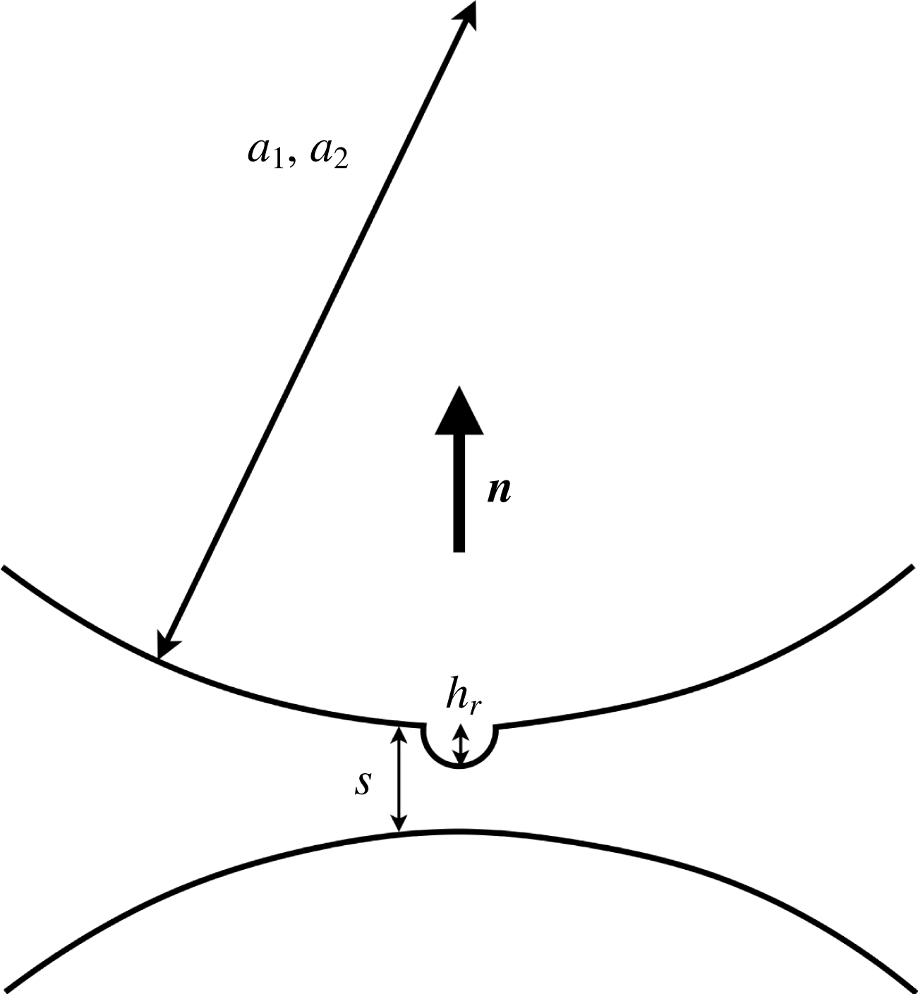
, and a smooth patch of the second particle (figure 1). In the original work of Brizmer et al. (Reference Brizmer, Kligerman and Etsion2007), the sphere was made of an elastic linear isotropic hardening material, where the Hooke and Prandtl–Reuss constitutive laws governed the elastic and plastic regimes, respectively. A normal preload
 $P$
was applied first and kept constant as the tangential load
 $Q$
was increased until sliding inception, which was treated as a plastic yield failure. The friction coefficient was defined as the ratio of the largest value of the tangential load
 $Q_{max}$
to the normal preload
 $P$
, and a correlation law was fitted to the variation of
 $Q_{max}$
with
 $P$
. Two different regimes were identified: when the preload is smaller than a critical value,
 $L_{c}$
(2.4), the deformation of the sphere keeps fully elastic during normal loading, and the friction coefficient decreases with the applied preload approximately as
 $(P/L_{c})^{-1/3}$
. As
 $P$
is increased, the fraction of the material that experiences plastic deformation increases and the friction coefficient gradually tends to a constant value. The correlation between the preload
 $P$
and the surface overlap is also provided, that includes the transition from elastic to plastic regime.
Sketch of the roughness modelling:
 $s$
is the hydrodynamic separation distance,
 $h_{r}$
is the roughness height.

In the present article, the contact force exerted on the smooth patch (figure 1) is split into the force normal to the surfaces,
 $\boldsymbol{F}_{n}$
, and the tangential force,
 $\boldsymbol{F}_{t}$
. The normal force depends on the surface overlap
 $\unicode[STIX]{x1D6FF}=h_{r}-s$
according to the correlation found by Brizmer, Kligerman & Etsion (Reference Brizmer, Kligerman and Etsion2006a
), Brizmer et al. (Reference Brizmer, Zait, Kligerman and Etsion2006b
), but, for the sake of simplicity, it is treated as fully elastic i.e. reversible. This means that the influence of the hysteresis of the contact law, which is connected to material plasticity, is neglected here. The normal force
 $\boldsymbol{F}_{n}$
is given in the elastic regime (
 $\unicode[STIX]{x1D6FF}\leqslant \unicode[STIX]{x1D6FF}_{c}$
,
 $L\leqslant L_{c}$
) by (2.3):
 $$\begin{eqnarray}\boldsymbol{F}_{n}=-L_{c}\left(\frac{\unicode[STIX]{x1D6FF}}{\unicode[STIX]{x1D6FF}_{c}}\right)^{3/2}\boldsymbol{n},\end{eqnarray}$$
where
 $L_{c}$
and
 $\unicode[STIX]{x1D6FF}_{c}$
are the critical normal load and surface overlap at yield inception, respectively:
 $$\begin{eqnarray}\displaystyle & \displaystyle L_{c}=\bar{L}_{c}\unicode[STIX]{x03C0}^{3}\frac{Y_{0}}{6}C_{\unicode[STIX]{x1D708}}^{3}\left(h_{r}\frac{2(1-\unicode[STIX]{x1D708}^{2})Y_{0}}{E}\right)^{2}, & \displaystyle\end{eqnarray}$$
 $$\begin{eqnarray}\displaystyle & \displaystyle \unicode[STIX]{x1D6FF}_{c}=\bar{\unicode[STIX]{x1D6FF}}_{c}h_{r}\left[\unicode[STIX]{x03C0}C_{\unicode[STIX]{x1D708}}\frac{(1-\unicode[STIX]{x1D708}^{2})Y_{0}}{E}\right]^{2}. & \displaystyle\end{eqnarray}$$
 $E$
,
 $\unicode[STIX]{x1D708}$
and
 $Y_{0}$
are Young’s modulus, Poisson’s ratio and the yield strength of the material, respectively, and
 $C_{\unicode[STIX]{x1D708}}=1.234+1.256\unicode[STIX]{x1D708}$
. Equations (2.3), (2.4) and (2.5) differ from the usual Hertz contact law between a sphere and a plane half-space made of the same material by the overbar quantities (2.6) and (2.7), that are characteristic of the full stick contact condition:
 $$\begin{eqnarray}\displaystyle & \displaystyle \bar{L}_{c}=[8.88\unicode[STIX]{x1D708}-10.13(\unicode[STIX]{x1D708}^{2}+0.089)], & \displaystyle\end{eqnarray}$$
 $$\begin{eqnarray}\displaystyle & \displaystyle \bar{\unicode[STIX]{x1D6FF}}_{c}=[6.82\unicode[STIX]{x1D708}-7.83(\unicode[STIX]{x1D708}^{2}+0.0586)]. & \displaystyle\end{eqnarray}$$
The case that was considered in the original articles of Brizmer et al. (Reference Brizmer, Kligerman and Etsion2006a
,Reference Brizmer, Zait, Kligerman and Etsion
b
, Reference Brizmer, Kligerman and Etsion2007) of a rigid flat surface was transposed to the present case of an elastic surface by considering that the relevant parameters for the contact between two spheres, 1 and 2, are the mean modulus
 $1/E^{\ast }=(1-\unicode[STIX]{x1D708}_{1}^{2})/E_{1}+(1-\unicode[STIX]{x1D708}_{1}^{2})/E_{2}=2(1-\unicode[STIX]{x1D708}^{2})/E$
and the mean curvature
 $1/R^{\ast }=1/R_{1}+1/R_{2}$
. This procedure is rigorously exact only for the elastic contact. In the present article, we only consider a contact between a spherical asperity with a radius
 $h_{r}$
and a flat surface, so that
 $1/R^{\ast }\approx 1/h_{r}$
.
In the plastic regime (
 $\unicode[STIX]{x1D6FF}>\unicode[STIX]{x1D6FF}_{c}$
,
 $L>L_{c}$
), the normal force is softer:
 $$\begin{eqnarray}\boldsymbol{F}_{n}=-L_{c}\left(\frac{\unicode[STIX]{x1D6FF}}{\unicode[STIX]{x1D6FF}_{c}}\right)^{3/2}\left[1-\exp \left(\frac{1}{1-\left({\displaystyle \frac{\unicode[STIX]{x1D6FF}}{\unicode[STIX]{x1D6FF}_{c}}}\right)^{\unicode[STIX]{x1D6FD}}}\right)\right]\boldsymbol{n},\end{eqnarray}$$
where
 $\unicode[STIX]{x1D6FD}=0.174+0.08\unicode[STIX]{x1D708}$
. In addition, due to the softness of the normal force, and the high level of contact forces at large shear rate and high solid volume fraction, particles may overlap, meaning that the asperity is fully flattened out, and the distance
 $s$
may become negative. To avoid this, a multiplying function is included, that goes to infinity for
 $s=0.2h_{r}$
(
 $\unicode[STIX]{x1D6FF}=0.8h_{r}$
), so that the distance between the particle surfaces,
 $s$
, is kept larger than 0.2
 $h_{r}$
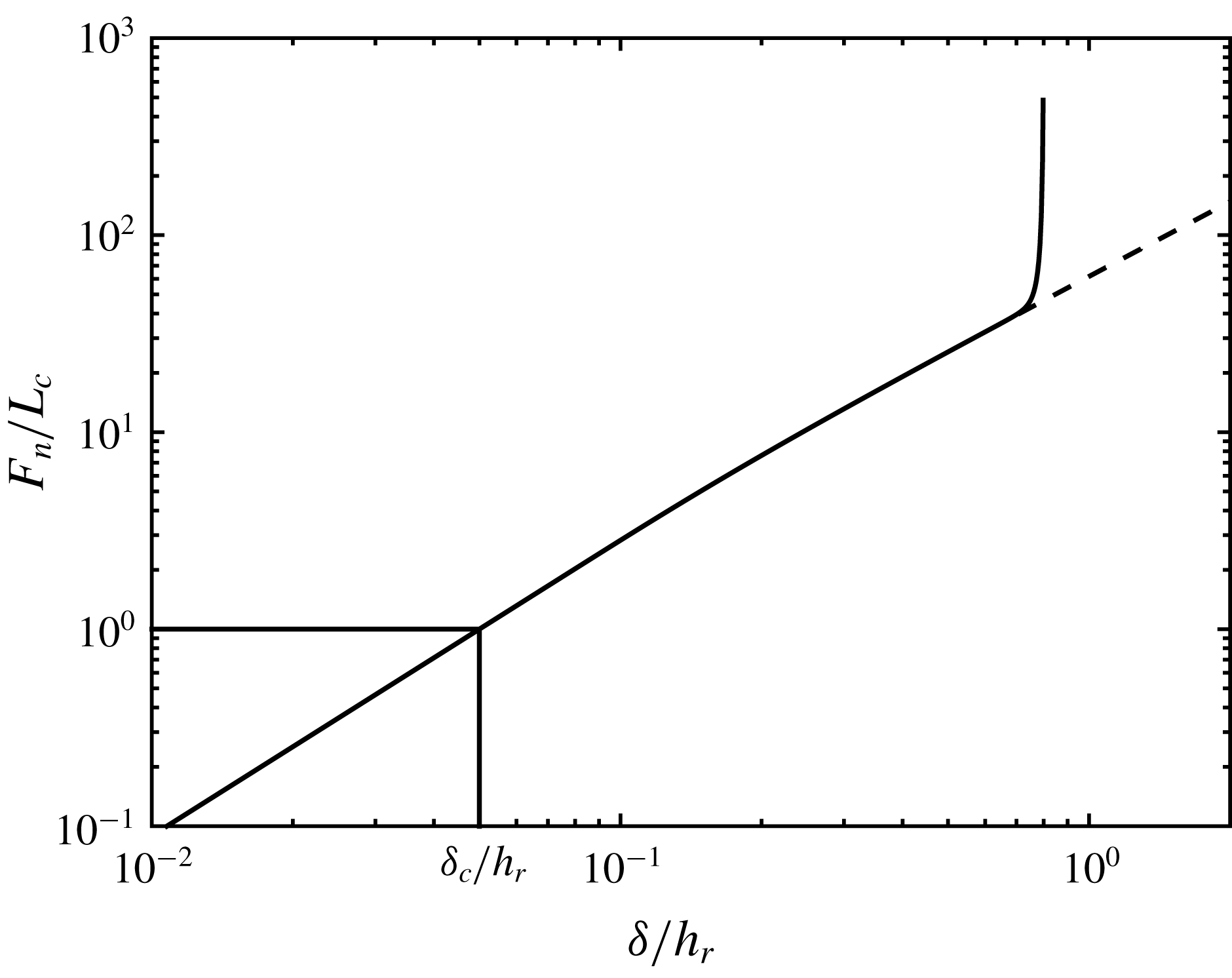
. This particular value was chosen arbitrarily but has only a quite weak influence on the lubrication stress. Figure 2 displays the interparticular force normalised by critical force
 $L_{c}$
as a function of the dimensionless overlap,
 $\unicode[STIX]{x1D6FF}/h_{r}$
. The dashed line is the dimensionless force from (2.8), while the solid line displays the force used in the simulations, in order to keep
 $\unicode[STIX]{x1D6FF}/h_{r}<0.8$
as mentioned above. Its expression differs from the original one only for
 $\unicode[STIX]{x1D6FF}/h_{r}\gtrsim 0.7$
.
Dimensionless normal contact force as a function of dimensionless overlap. Dashed line: original force from (2.8). Solid line: corrected force to keep
 $\unicode[STIX]{x1D6FF}/h_{r}<0.8$
.

The tangential force is modelled as a linear spring-like force with a threshold as in Cundall & Strack (Reference Cundall and Strack1979), Gallier et al. (Reference Gallier, Lemaire, Peters and Lobry2014), Peters et al. (Reference Peters, Ghigliotti, Gallier, Blanc, Lemaire and Lobry2016):
 $$\begin{eqnarray}\boldsymbol{F}_{t}=\left\{\begin{array}{@{}ll@{}}-\unicode[STIX]{x1D705}_{t}{\mathcal{Y}}\quad & \text{for}~|\boldsymbol{F}_{t}|<\unicode[STIX]{x1D707}|\boldsymbol{F}_{n}|\text{(stick-phase)}\\ \unicode[STIX]{x1D707}|\boldsymbol{F}_{n}|{\displaystyle \frac{\boldsymbol{F}_{t}}{|\boldsymbol{F}_{t}|}}\quad & \text{otherwise (slip-phase)},\end{array}\right.\end{eqnarray}$$
where
 $\unicode[STIX]{x1D707}$
is the (static and dynamic) friction coefficient.
 ${\mathcal{Y}}$
is the relative tangential displacement of the two particle surfaces and it is calculated as the integral of the slip velocity during contact (Peters et al.
Reference Peters, Ghigliotti, Gallier, Blanc, Lemaire and Lobry2016). The value of the stiffness of the tangential spring,
 $\unicode[STIX]{x1D705}_{t}$
, is linked to the normal force intensity
 $|\boldsymbol{F}_{n}|$
through (2.10) so that it depends on the surface overlap
 $\unicode[STIX]{x1D6FF}$
(2.8).
 $$\begin{eqnarray}\unicode[STIX]{x1D705}_{t}=\frac{2}{7}\frac{|\boldsymbol{F}_{n}|}{\unicode[STIX]{x1D6FF}}.\end{eqnarray}$$
The friction coefficient has been computed by Brizmer et al. (Reference Brizmer, Kligerman and Etsion2007) as:
 $$\begin{eqnarray}\unicode[STIX]{x1D707}=0.27\coth \left[0.27\left(\frac{|\boldsymbol{F}_{n}|}{L_{c}}\right)^{0.35}\right].\end{eqnarray}$$
The last equations deserve a few comments. Firstly, the tangential force in the stick phase, as defined in (2.9) and (2.10), is an approximate version of the original model by Brizmer et al. (Reference Brizmer, Kligerman and Etsion2007). In the present paper, the tangential force (2.9) is assumed to be linear with the tangential displacement, while in the original work of Brizmer et al. (Reference Brizmer, Kligerman and Etsion2007), the material undergoes plastic deformation, and the force does not depend on the tangential displacement in a strict linear way. In addition, the coefficient
 $2/7$
is smaller than the value
 $3(1-\unicode[STIX]{x1D708})/(2-\unicode[STIX]{x1D708})$
that may be estimated from Brizmer et al. (Reference Brizmer, Kligerman and Etsion2007). It is chosen here mostly to be consistent with earlier work (Gallier et al.
Reference Gallier, Lemaire, Peters and Lobry2014; Peters et al.
Reference Peters, Ghigliotti, Gallier, Blanc, Lemaire and Lobry2016). This particular value was originally chosen to fit experimental data from impact experiments (Shäfer, Dippel & Wolf Reference Shäfer, Dippel and Wolf1996).
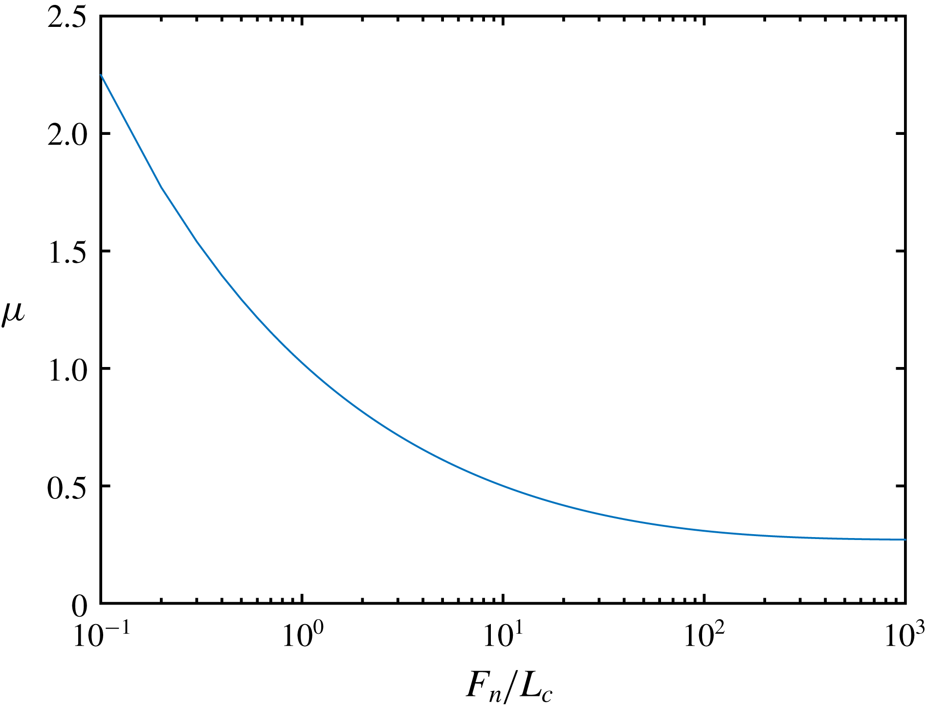
The most important feature of the model, at least for the present work, is displayed in (2.11), which is that the friction coefficient decreases as the normal force increases and reaches a plateau at high load. The variation of
 $\unicode[STIX]{x1D707}$
is plotted in figure 3. In the elastic regime (
 $F_{n}/L_{c}<1$
), equation (2.11) yields
 $\unicode[STIX]{x1D707}\propto (L_{c}/F_{n})^{0.35}$
in approximate agreement with Hertz theory according to which the contact area is determined by the normal force
 $A\propto F_{n}^{2/3}$
. Indeed, since sliding inception is modelled as a plastic yield failure, it occurs as the tangential force exceeds
 $F_{t}^{max}\propto Y_{0}A\propto Y_{0}F_{n}^{2/3}$
, leading to
 $\unicode[STIX]{x1D707}=F_{t}^{max}/F_{n}\propto F_{n}^{-1/3}\sim F_{n}^{-0.35}$
. As the dimensionless normal force
 $F_{n}/L_{c}$
increases far beyond 1, the material in the whole contact zone undergoes plastic deformation, and the contact area is proportional to the normal force, giving the constant friction coefficient
 $\unicode[STIX]{x1D707}=0.27$
. This particular value depends weakly on the material properties (Brizmer et al.
Reference Brizmer, Kligerman and Etsion2007).
Friction coefficient as a function of dimensionless contact normal force (2.11).

2.2.4 Dimensionless parameters
From the microscopic model presented in the last sections, several dimensionless parameters can be identified from the relevant length scales
 $a_{1}$
,
 $a_{2}$
,
 $h_{r}$
,
 $\unicode[STIX]{x1D6FF}_{c}$
and force scales
 $L_{c}$
,
 $6\unicode[STIX]{x03C0}\unicode[STIX]{x1D702}_{0}a_{1}^{2}\dot{\unicode[STIX]{x1D6FE}}$
. The latter is approximately the largest interparticle force experienced by two contacting particles of radius
 $a_{1}$
in a sheared dilute suspension. The value that we chose for the ratio of the roughness height to the smallest radius
 $h_{r}/a_{1}=5\times 10^{-3}$
is typical for polymer spheres model suspensions (Blanc et al.
Reference Blanc, Peters and Lemaire2011; Moon et al.
Reference Moon, Dai, Chang, Lee and Tanner2015). The interparticle force is completely specified by the critical force
 $L_{c}$
and the critical overlap
 $\unicode[STIX]{x1D6FF}_{c}$
, so that the relevant dimensionless parameters are the dimensionless shear rate defined as:
 $$\begin{eqnarray}\dot{\unicode[STIX]{x1D6E4}}=\frac{6\unicode[STIX]{x03C0}\unicode[STIX]{x1D702}_{0}a_{1}^{2}\dot{\unicode[STIX]{x1D6FE}}}{L_{c}}\end{eqnarray}$$
and the ratio of the critical overlap to the roughness height
 $\unicode[STIX]{x1D6FF}_{c}/h_{r}$
.
In addition, in dilute suspensions, the interparticle force level is
 $F_{n}\sim 6\unicode[STIX]{x03C0}\unicode[STIX]{x1D702}_{0}a_{1}^{2}\dot{\unicode[STIX]{x1D6FE}}$
, so that the value of the reduced shear rate
 $\dot{\unicode[STIX]{x1D6E4}}$
determines the typical overlap (figure 2) and the typical friction coefficient
 $\unicode[STIX]{x1D707}$
(figure 3). When
 $\dot{\unicode[STIX]{x1D6E4}}\ll$
1, the contact is mainly elastic (
 $\unicode[STIX]{x1D6FF}<\unicode[STIX]{x1D6FF}_{c}$
) and the typical friction coefficient decreases with shear rate, while the contact is mainly plastic and the typical friction coefficient tends to a plateau as
 $\dot{\unicode[STIX]{x1D6E4}}\gg$
1 (
 $\unicode[STIX]{x1D6FF}\gg \unicode[STIX]{x1D6FF}_{c}$
).
Typical values of physical parameters.

Table 1 gathers numerical values for different parameters computed for polystyrene for usual values of the shear rate
 $\dot{\unicode[STIX]{x1D6FE}}$
. Most importantly, the reduced shear rate
 $\dot{\unicode[STIX]{x1D6E4}}$
ranges from
 $4\times 10^{-3}$
to
 $4\times 10^{1}$
, meaning that the contacting material behaviour is expected to switch from elastic to plastic as the shear rate is increased. In addition, the initially decreasing friction coefficient will level off at high shear rate.
The small value of the ratio
 $\unicode[STIX]{x1D6FF}_{c}/h_{r}$
indicates that the roughness deformation at yield inception is very low, and supports the idea of a mono- or few-asperity contact, at least for
 $\dot{\unicode[STIX]{x1D6E4}}\lesssim 1$
. It is also possible to evaluate the number of asperities that come into contact as a first asperity is compressed with
 $\unicode[STIX]{x1D6FF}=\unicode[STIX]{x1D6FF}_{c}$
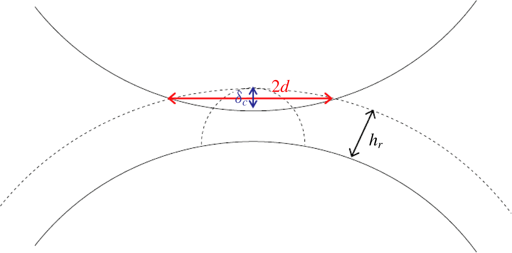
. The asperities likely to come into contact are those which are on the surface of a spherical cap of radius
 $d$
(see figure 4) where
 $d$
is the radius of the circle defined by the intersection of the two spheres of radius
 $a_{1}$
and
 $a_{1}+h_{r}$
whose centres are separated by a distance
 $2a_{1}+h_{r}-\unicode[STIX]{x1D6FF}_{c}$
. We then obtain that
 $d^{2}\approx \unicode[STIX]{x1D6FF}_{c}a_{1}$
or
 $d/h_{r}\approx \sqrt{(\unicode[STIX]{x1D6FF}_{c}/h_{r})(a_{1}/h)_{r}}\approx 1.4$
suggesting again a small number of compressed asperities.
Sketch of the contact;
 $d$
is the distance from a compressed asperity to the furthest compressed asperity.

The Reynolds number
 $Re=\dot{\unicode[STIX]{x1D6FE}}a_{1}^{2}\unicode[STIX]{x1D70C}/\unicode[STIX]{x1D702}_{0}$
is estimated from the values in table 1, using also the typical values of the viscosity
 $\unicode[STIX]{x1D702}_{0}=0.5$
Pa s and density
 $\unicode[STIX]{x1D70C}=1~\text{g}~\text{cm}^{-3}$
, which are close to the values in our experimental system (§ 4).
 $Re<8\times 10^{-5}$
, so that inertia can be safely neglected.
2.3 Simulation parameters
From a practical point of view, the variety of the length scales [
 $\unicode[STIX]{x1D6FF}_{c}$
;
 $h_{r}$
;
 $a_{1}$
] is quite difficult to deal with in computations, since very small time steps are required to accurately compute the contact dynamics, and quite long deformation is needed for correct averaging. To keep the time step reasonably large (i.e. larger than
 $10^{-6}$
in strain units), we set the critical length ratio
 $\unicode[STIX]{x1D6FF}_{c}/h_{r}=5\times 10^{-2}$
.
Finally, table 2 gathers the simulation parameters. Besides suspensions of particles displaying a load-dependent friction coefficient, suspensions made of particles with constant friction coefficient have been considered as well in another set of simulations for comparison. The microscopic model is strictly the same, except for (2.11).
Simulation parameters.

3 Simulation results
In this section, the shear stress and the viscosity are investigated. The normal stress differences are shortly studied in the first appendix at the end of the article, and some elements concerning contact force statistics are given in appendix B.
3.1 Constant friction coefficient
Before we address the issue of particles with load-dependent friction coefficient, we first present simulations where
 $\unicode[STIX]{x1D707}$
is kept constant. This will be our opportunity to recall the great influence of this microscopic parameter on the suspension viscosity, as well as to derive correlation laws from the simulations that will help quantitatively with our understanding of the more original case of load-dependent friction.
Quite recent numerical studies concerning frictional non-Brownian suspensions demonstrated a strong influence of the friction coefficient
 $\unicode[STIX]{x1D707}$
, taken as a constant, on the effective viscosity (Gallier et al.
Reference Gallier, Lemaire, Peters and Lobry2014; Mari et al.
Reference Mari, Seto, Morris and Denn2014; Peters et al.
Reference Peters, Ghigliotti, Gallier, Blanc, Lemaire and Lobry2016; Gallier, Peters & Lobry Reference Gallier, Peters and Lobry2018; Singh et al.
Reference Singh, Mari, Denn and Morris2018). The key feature here is that the jamming volume fraction significantly depends on the friction coefficient. For instance, Mari et al. (Reference Mari, Seto, Morris and Denn2014), in their study of concentrated discontinuous shear-thickening suspensions, computed the high shear rate jamming volume fraction
 $\unicode[STIX]{x1D719}_{m}$
for three values of the microscopic friction coefficient, namely
 $\unicode[STIX]{x1D707}=0$
,
 $\unicode[STIX]{x1D707}=1$
and
 $\unicode[STIX]{x1D707}=\infty$
. The jamming volume fraction was shown to decrease from
 $0.66$
to
 $0.56$
. More recently, Peters et al. (Reference Peters, Ghigliotti, Gallier, Blanc, Lemaire and Lobry2016) and Singh et al. (Reference Singh, Mari, Denn and Morris2018) explained the variation of the viscosity of non-colloidal suspensions with the microscopic particle friction coefficient by a smooth decrease of the jamming volume fraction for microscopic friction coefficient ranging from
 $0$
to
 $1$
. We note that such a correlation between jamming volume fraction and microscopic friction coefficient was evidenced in simulations of granular flows (Silbert Reference Silbert2010) and in experiments concerning discontinuous shear-thickening suspensions (Fernandez et al.
Reference Fernandez, Mani, Rinaldi, Kadau, Mosquet, Lombois-Burger, Cayer-Barrioz, Herrmann, Spencer and Isa2013; Chatté et al.
Reference Chatté, Comtet, Niguès, Bocquet, Siria, Ducouret, Lequeux, Lenoir, Ovarlez and Colin2018).
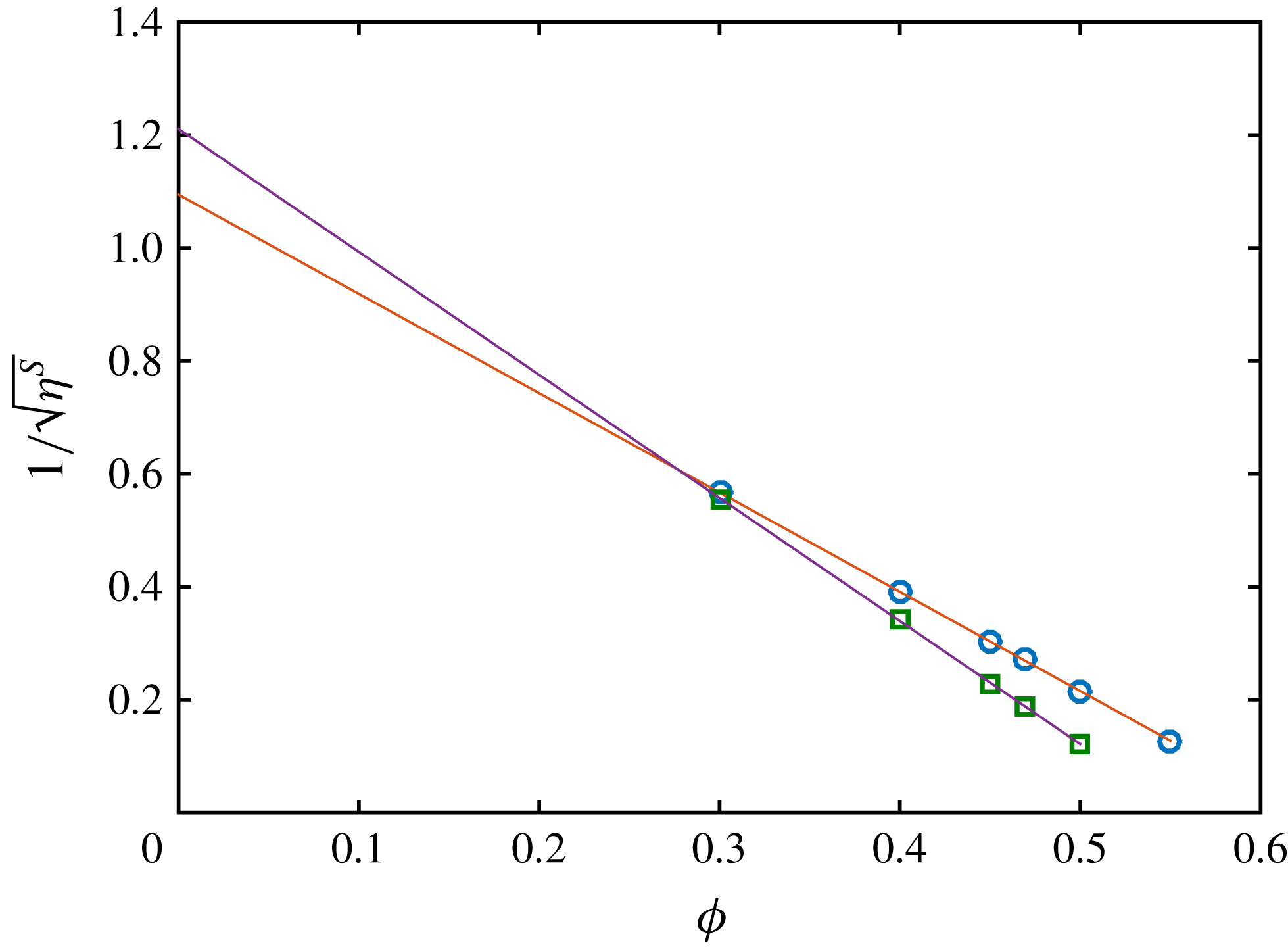
We show here similar simulations where the friction coefficient is kept constant (table 2). For each value of
 $\unicode[STIX]{x1D707}$
, the following simple correlation law is fitted to the variation of the relative viscosity against the volume fraction:
 $$\begin{eqnarray}\unicode[STIX]{x1D702}^{S}(\unicode[STIX]{x1D707},\unicode[STIX]{x1D719})=\frac{\unicode[STIX]{x1D6FC}_{0}(\unicode[STIX]{x1D707})}{\left(1-{\displaystyle \frac{\unicode[STIX]{x1D719}}{\unicode[STIX]{x1D719}_{m}(\unicode[STIX]{x1D707})}}\right)^{2}}.\end{eqnarray}$$
We note that such a fitting function has already been used in recent works concerning concentrated suspensions (Peters et al.
Reference Peters, Ghigliotti, Gallier, Blanc, Lemaire and Lobry2016; Singh et al.
Reference Singh, Mari, Denn and Morris2018). Obviously, the correlation (3.1) is not suitable at low volume fraction, for which the value
 $\unicode[STIX]{x1D6FC}_{0}=1$
is expected. The data from the simulation together with the respective correlation laws are displayed in figure 5 for two values of the friction coefficient.
Inverse of the square root of the shear viscosity against volume fraction for two values of the friction coefficient. (○)
 $\unicode[STIX]{x1D707}=0.27$
(▫)
 $\unicode[STIX]{x1D707}=2$
. Solid lines: best fit of (3.1) to the data. The variation of
 $\unicode[STIX]{x1D719}_{max}$
and
 $\unicode[STIX]{x1D6FC}_{0}$
with
 $\unicode[STIX]{x1D707}$
is clearly displayed.


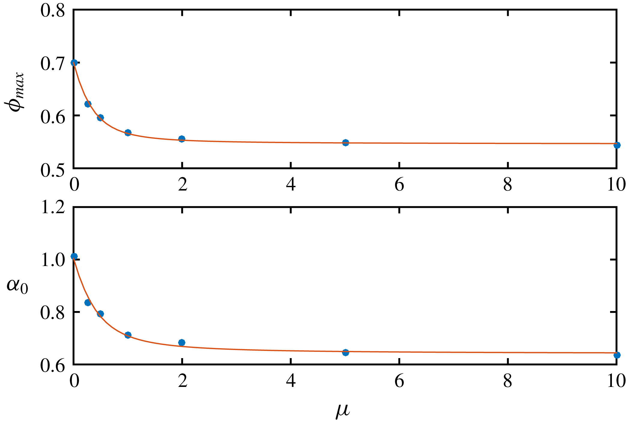
The fitting parameters
 $\unicode[STIX]{x1D6FC}_{0}$
and
 $\unicode[STIX]{x1D719}_{m}$
are displayed in figure 6 against the friction coefficient
 $\unicode[STIX]{x1D707}$
, together with the best fit to equations (3.2), where the
 $\unicode[STIX]{x1D719}_{m}^{x}$
,
 $\unicode[STIX]{x1D6FC}_{0}^{x}$
and
 $X^{x}$
are again fitting parameters, that are gathered in table 3.
 $$\begin{eqnarray}\begin{array}{@{}l@{}}\unicode[STIX]{x1D719}_{m}=\unicode[STIX]{x1D719}_{m}^{\infty }+(\unicode[STIX]{x1D719}_{m}^{0}-\unicode[STIX]{x1D719}_{m}^{\infty }){\displaystyle \frac{\exp (-X^{p}\text{atan}(\unicode[STIX]{x1D707}))-\exp (-\unicode[STIX]{x03C0}X^{p}/2)}{1-\exp (-\unicode[STIX]{x03C0}X^{p}/2)}}\\ \unicode[STIX]{x1D6FC}_{0}=\unicode[STIX]{x1D6FC}_{0}^{\infty }+(\unicode[STIX]{x1D6FC}_{0}^{0}-\unicode[STIX]{x1D6FC}_{0}^{\infty }){\displaystyle \frac{\exp (-X^{a}\text{atan}(\unicode[STIX]{x1D707}))-\exp (-\unicode[STIX]{x03C0}X^{a}/2)}{1-\exp (-\unicode[STIX]{x03C0}X^{a}/2)}}\end{array}.\end{eqnarray}$$
Fitting parameters of (3.2).

In particular, the jamming volume fraction seems to approach the limit
 $\unicode[STIX]{x1D719}_{m}^{\infty }=0.546$
as the friction coefficient goes to
 $\infty$
and is equal to
 $\unicode[STIX]{x1D719}_{m}^{0}=0.700$
for
 $\unicode[STIX]{x1D707}=0$
. These values are somewhat different from the values that can be found in the literature and that have been obtained from simulations performed at higher volume fraction. It is especially true for frictionless particles where the jamming fraction was estimated to be approximately
 $0.64$
for
 $\unicode[STIX]{x1D707}=0$
(Mari et al.
Reference Mari, Seto, Morris and Denn2014; Gallier et al.
Reference Gallier, Peters and Lobry2018; Singh et al.
Reference Singh, Mari, Denn and Morris2018). This is not really a problem in the present article, since the fitting functions in (3.1) and (3.2) properly describe the simulation data in the volume fraction range that is kept throughout the study. In addition, our data are in quite good agreement with measurements performed with discontinuous shear-thickening suspensions in the frictional regime (Fernandez et al.
Reference Fernandez, Mani, Rinaldi, Kadau, Mosquet, Lombois-Burger, Cayer-Barrioz, Herrmann, Spencer and Isa2013). Concerning
 $\unicode[STIX]{x1D6FC}_{0}$
, inspection of figure 6 shows that its variation with the friction coefficient is correlated with the variation of
 $\unicode[STIX]{x1D719}_{m}$
. This can be easily understood, noting that the viscosity from the simulations for any volume fraction lower than
 $0.3$
hardly depends on the friction coefficient, so that the variation of
 $\unicode[STIX]{x1D719}_{m}$
has to be balanced by the variation of
 $\unicode[STIX]{x1D6FC}_{0}$
in this volume fraction range. Finally, even though
 $\unicode[STIX]{x1D6FC}_{0}$
significantly decreases with the friction coefficient, the viscosity variations for sufficiently high volume fraction are mostly due to the variation of
 $\unicode[STIX]{x1D719}_{m}$
.
3.2 Load-dependent friction coefficient
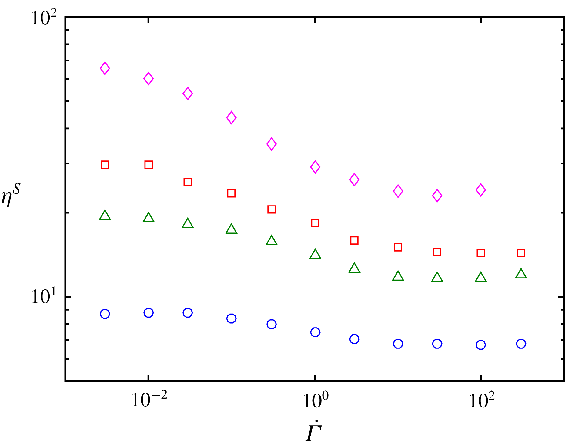
Relative viscosity as a function of the reduced shear rate. (○)
 $\unicode[STIX]{x1D719}=40\,\%$
, (▵)
 $\unicode[STIX]{x1D719}=45\,\%$
, (▫)
 $\unicode[STIX]{x1D719}=47\,\%$
, (♢)
 $\unicode[STIX]{x1D719}=50\,\%$
.

Figure 7 displays the computed relative viscosity as a function of the reduced shear rate
 $\dot{\unicode[STIX]{x1D6E4}}$
. As expected, as the reduced shear rate increases, the viscosity decreases, due to friction coefficient reduction. The viscosity exhibits two plateaus, one at low reduced shear rate and the other at high reduced shear rate. The latter is due to the saturation of the friction coefficient as
 $F_{n}/L_{c}$
increases. The low shear plateau originates in the saturation of the viscosity as the friction coefficient increases. More quantitatively, as recently shown for monodisperse suspensions (Peters et al.
Reference Peters, Ghigliotti, Gallier, Blanc, Lemaire and Lobry2016) and in more detail in the following, the friction coefficient has a strong influence on the viscosity only in a range of roughly [0;1–2]. In the present model, the friction coefficient may vary in the range [0.27;
 $+\infty$
] depending on the normal force between particles. For moderately concentrated suspensions, it is thus expected from figure 3 that the viscosity mostly varies when the reduced shear rate
 $\dot{\unicode[STIX]{x1D6E4}}$
(2.12) ranges from
 $10^{-1}$
to 10. This is approximately the case for the lowest volume fraction
 $\unicode[STIX]{x1D719}=40\,\%$
, and as the volume fraction increases, the curves shift toward lower reduced shear rate. This is expected, since the viscosity and more generally the stress level increase as
 $\unicode[STIX]{x1D719}$
increases, yielding a stronger contact force between particles at the same value of
 $\dot{\unicode[STIX]{x1D6E4}}$
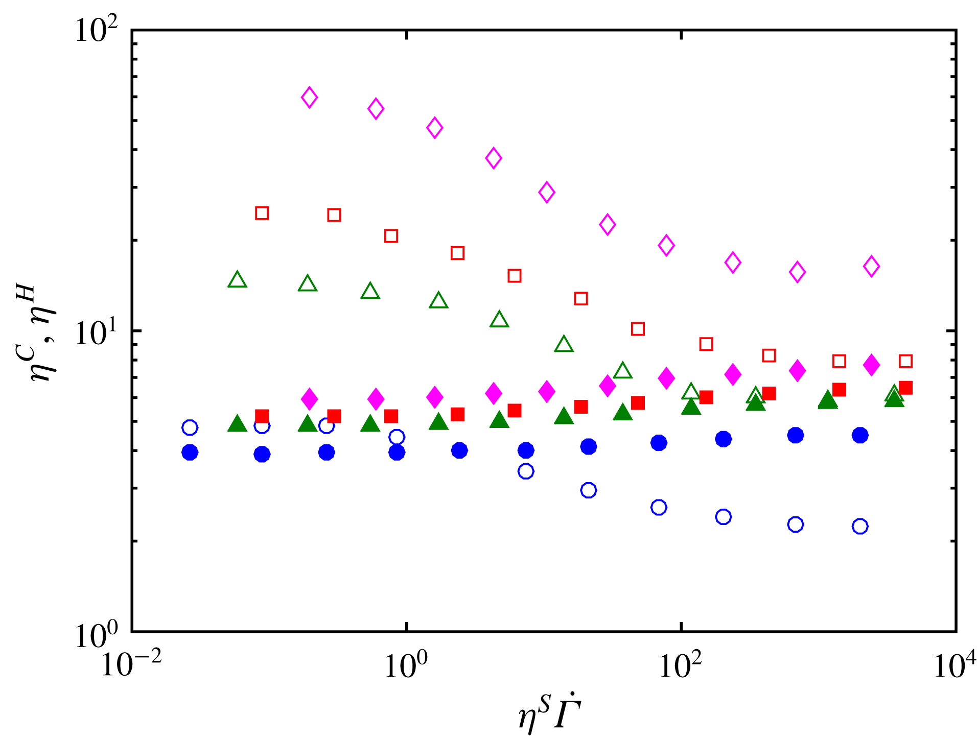
. It is also instructive to split the viscosity into the hydrodynamic and contact contributions, as displayed in figure 8. While the contact contribution features shear-thinning behaviour, the hydrodynamic part weakly increases as the reduced shear rate increases. This can be qualitatively understood, considering that the typical surface separation between contacting particles decreases, due to contact elasticity, leading to stronger lubrication interactions. Such a feature has already been noted for constant friction coefficient particles as the surface roughness height was varied (Gallier et al.
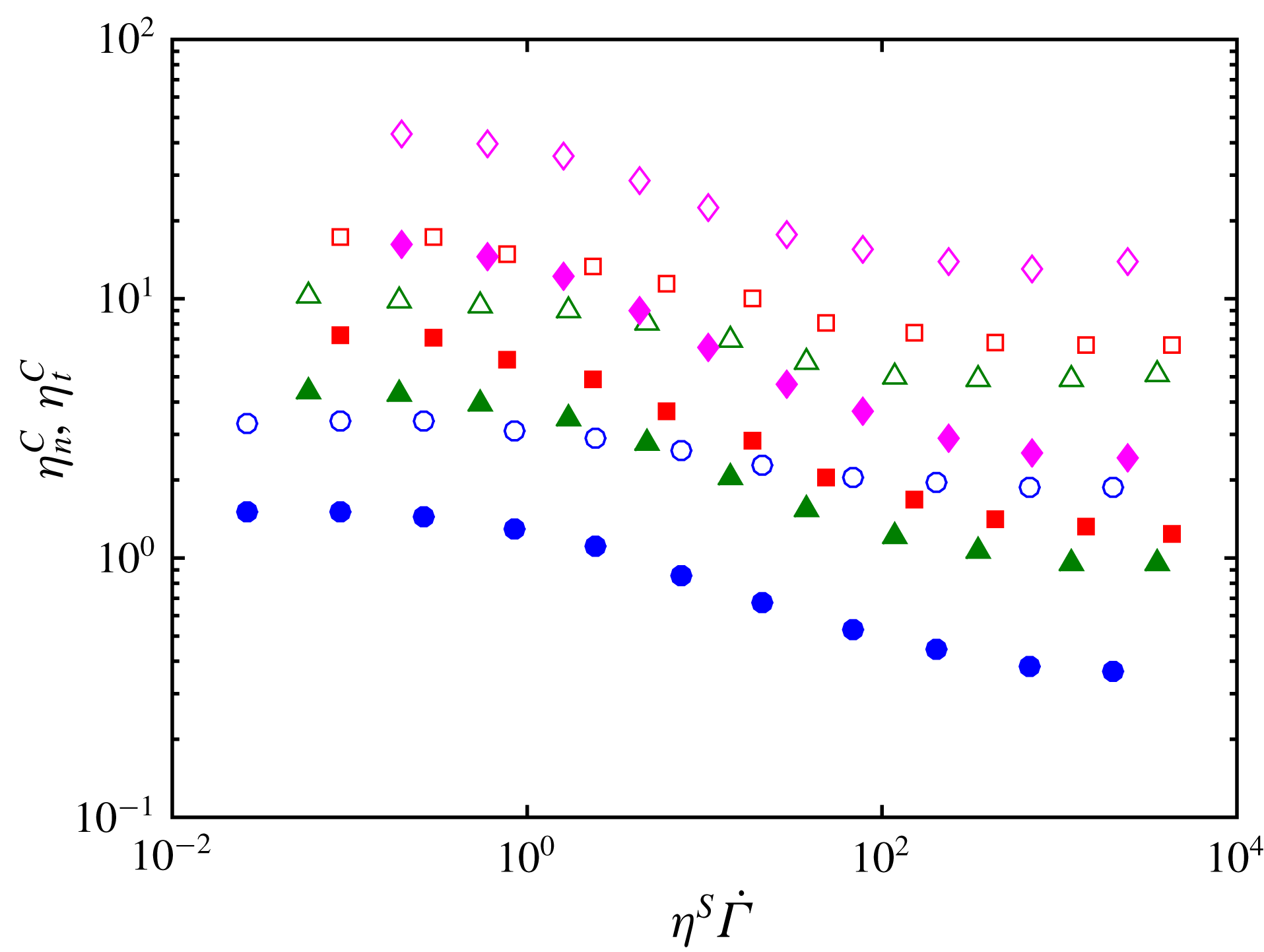
Reference Gallier, Lemaire, Peters and Lobry2014). In figure 9, the contact contribution is further split into the normal and tangential force contributions. The tangential force contribution is shown to undergo stronger decrease as the reduced shear rate increases compared to the normal force contribution. Again, this can be understood based on previous simulations of suspensions with a constant friction coefficient (Peters et al.
Reference Peters, Ghigliotti, Gallier, Blanc, Lemaire and Lobry2016), where the decrease of the friction coefficient leads to the decrease of the ratio between the tangential to normal force contributions. As a consequence, in the present study, as the reduced shear rate increases, the ratio of the tangential to normal force contribution decreases so that the decrease of the tangential force contribution is amplified compared to the normal force contribution.
Hydrodynamic and contact contributions to the viscosity. Open symbols: contact contribution. Closed symbols: hydrodynamic contribution. Same volume fraction values as in figure 7.

Normal and tangential contact force contributions to the viscosity. Open symbols: normal force contribution. Closed symbols: tangential force contribution. Same volume fraction values as in figure 7.

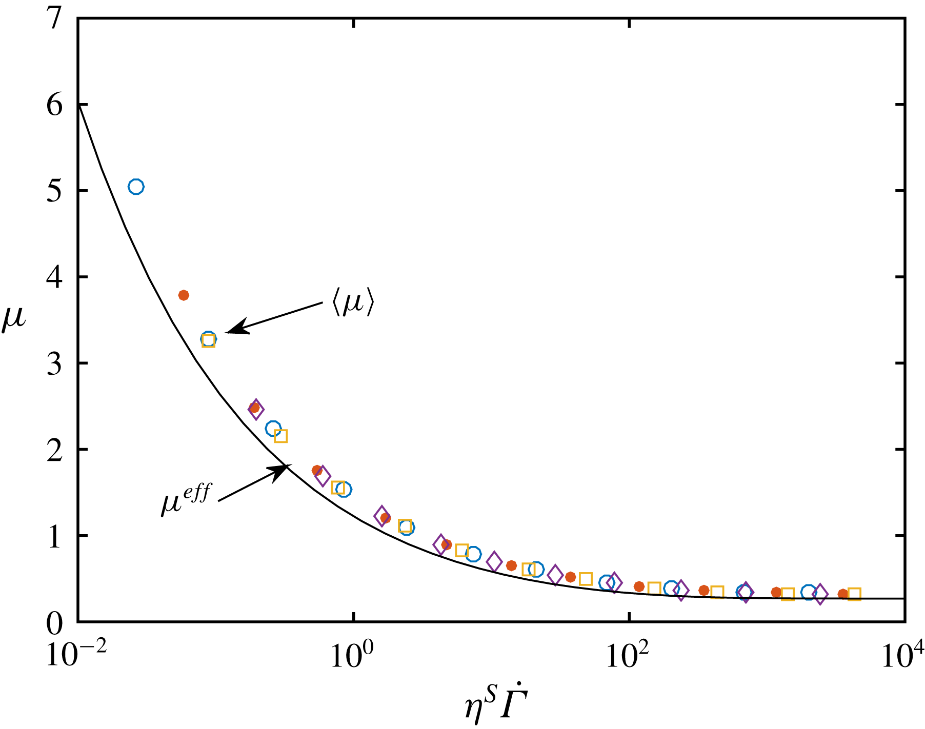
To gain a deeper insight into this transition from high to low viscosity, the mean friction coefficient,
 $\langle \unicode[STIX]{x1D707}\rangle$
, over all contacting particle pairs is displayed in figure 10 as a function of the reduced shear stress,
 $\unicode[STIX]{x1D702}^{S}\dot{\unicode[STIX]{x1D6E4}}$
, which quantifies the typical force experienced by two contacting particles. A striking feature is that the data collapse on a single curve whatever the particle volume fraction. This feature is not completely obvious and deserves a comment. The microscopic friction coefficient between contacting particles is indeed controlled by the actual normal contact force. However, the mean force is only qualitatively connected to the bulk shear stress. In addition, the contact force distribution is quite broad, with a distribution width which is comparable to the mean force (Gallier Reference Gallier2014) and may depend on the volume fraction. Since the relation between microscopic friction coefficient and force is highly nonlinear, even the relation between mean friction coefficient and mean force is not easy to anticipate. On the whole, it means that the reduced shear stress can be understood as the reduced effective normal force between contacting particles that controls the mean friction coefficient. The model built in § 3.3 is based on this idea.
Symbols: friction coefficient averaged over all contacting particle pairs. (○)
 $\unicode[STIX]{x1D719}=40\,\%$
(●)
 $\unicode[STIX]{x1D719}=45\,\%$
▫
 $\unicode[STIX]{x1D719}=47\,\%$
♢
 $\unicode[STIX]{x1D719}=50\,\%$
. Solid line: effective friction coefficient from (3.4).

3.3 Viscosity model
In this section, we show that a simple model based on the correlation laws from the simulations with constant friction coefficient described in § 3.1 allows us to precisely reproduce the viscosity that is simulated when the load-dependent friction is taken into account. Returning to the particles with a load-dependent friction coefficient, we make the assumption that the viscosity can be computed from (3.1) and (3.2), provided that the relevant effective friction coefficient,
 $\unicode[STIX]{x1D707}^{eff}$
, is controlled by the reduced shear stress as proposed in § 3.2 and supported by the collapse of the mean friction coefficient with
 $\unicode[STIX]{x1D702}^{S}\dot{\unicode[STIX]{x1D6E4}}$
(figure 10). We note that this approach is quite similar to that recently followed by Chatté et al. (Reference Chatté, Comtet, Niguès, Bocquet, Siria, Ducouret, Lequeux, Lenoir, Ovarlez and Colin2018) to explain their experimental results. Therefore, we obtain the following self-consistent expression for the shear-thinning suspension viscosity:
 $$\begin{eqnarray}\unicode[STIX]{x1D702}^{S}(\dot{\unicode[STIX]{x1D6E4}},\unicode[STIX]{x1D719})=\frac{\unicode[STIX]{x1D6FC}_{0}(\unicode[STIX]{x1D707}^{eff}(\unicode[STIX]{x1D702}^{S}\dot{\unicode[STIX]{x1D6E4}}))}{\left(1-{\displaystyle \frac{\unicode[STIX]{x1D719}}{\unicode[STIX]{x1D719}_{m}(\unicode[STIX]{x1D707}^{eff}(\unicode[STIX]{x1D702}^{S}\dot{\unicode[STIX]{x1D6E4}}))}}\right)^{2}}.\end{eqnarray}$$
A very good prediction of the viscosity–shear stress behaviour is obtained if the following expression of the effective friction coefficient is introduced in (3.3):
 $$\begin{eqnarray}\unicode[STIX]{x1D707}^{eff}=0.27\coth \left[0.27\left(\frac{\unicode[STIX]{x1D702}^{S}\dot{\unicode[STIX]{x1D6E4}}}{1.69}\right)^{0.35}\right],\end{eqnarray}$$
where the scaling factor 1.69 has been tuned in order for the model to fit the simulation data. The computed viscosity from (3.2), (3.3) and (3.4) is displayed in figure 11, and is in close agreement with the data from the simulation. It follows from this phenomenological model that the characteristic reduced force that controls friction, and consequently the suspension viscosity, is proportional to the reduced shear stress:
 $$\begin{eqnarray}\frac{\bar{F}_{n}}{L_{c}}=\frac{6\unicode[STIX]{x03C0}\unicode[STIX]{x1D702}_{0}\unicode[STIX]{x1D702}^{S}a_{1}^{2}\dot{\unicode[STIX]{x1D6FE}}}{1.69L_{c}}=\frac{\unicode[STIX]{x1D702}^{S}\dot{\unicode[STIX]{x1D6E4}}}{1.69}.\end{eqnarray}$$
It should be noted (figure 10) that the effective friction coefficient,
 $\unicode[STIX]{x1D707}^{eff}$
, which has been tuned in order for the modelled viscosity to fit the simulated viscosity, shows shear stress behaviour that is quite close to the mean friction coefficient,
 $\langle \unicode[STIX]{x1D707}\rangle$
, a direct output of the simulations (§ 3.2).

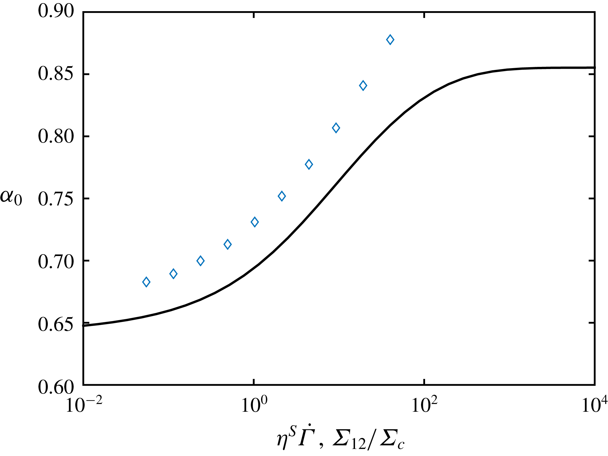
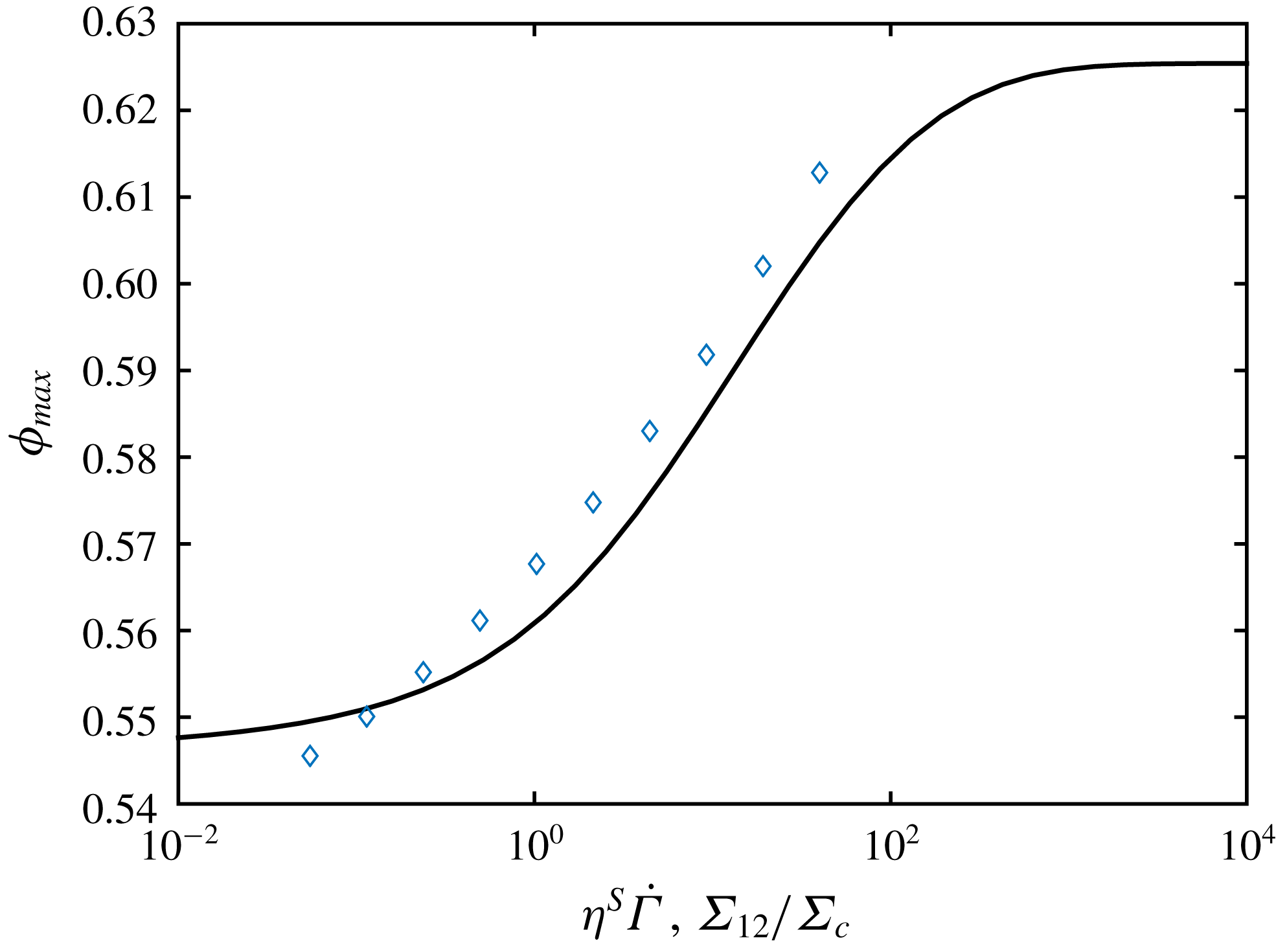
Using (3.2) and (3.4), we can compute the variation of
 $\unicode[STIX]{x1D6FC}_{0}$
(solid line in figure 12) and
 $\unicode[STIX]{x1D719}_{m}$
(solid line in figure 13) with
 $\unicode[STIX]{x1D702}_{S}\dot{\unicode[STIX]{x1D6E4}}$
. At low shear stress, where the friction coefficient diverges, the jamming volume fraction approaches the asymptotic value
 $\unicode[STIX]{x1D719}_{m}^{\infty }=0.546$
for high friction coefficient ((3.2) and text thereafter). At high shear stress,
 $\unicode[STIX]{x1D719}_{m}$
levels off at the value
 $0.625$
computed from (3.2) for the lowest friction coefficient
 $0.27$
corresponding to infinite shear stress (3.4).


To conclude this numerical section, it should be noted that the very good agreement between the data from the load-dependent friction simulations and the viscosity from (3.3) allows us to check the influence of any particular friction law on the viscosity without the need to perform new simulations. We follow this idea at the end of the experimental section.
4 Experiments
4.1 Suspensions
The suspensions are made of polystyrene (PS) particles (Dynoseed TS40, Microbeads), dispersed in silicon oil (M 500, Roth). The particles are
 $40~\unicode[STIX]{x03BC}\text{m}$
in diameter with a relative standard deviation lower than
 $5\,\%$
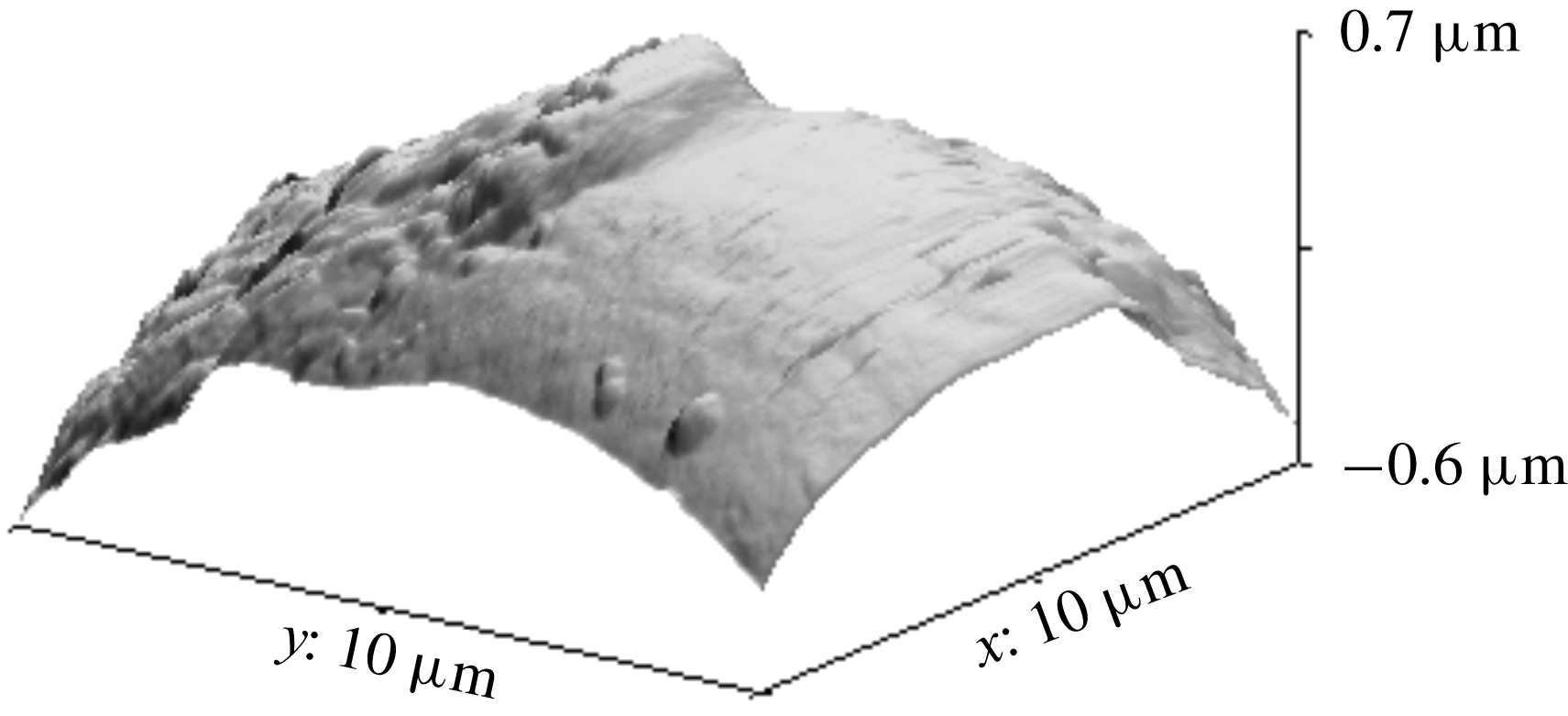
. Their roughness has been measured using an atomic force microscope (AFM) (see figure 14) and has been found to be around 36 nm (root-mean-square value) which agrees closely with the results of Moon et al. (Reference Moon, Dai, Chang, Lee and Tanner2015), who measured 32 nm, and not so far from the estimation of Garland et al. (Reference Garland, Gauthier, Martin and Morris2013), who measured a characteristic roughness height around 100 nm. Before adding the particles to the suspending liquid, they are carefully washed with clear water and dried under vacuum at
 $60\,^{\circ }\text{C}$
for 12 h.
AFM image of a polystyrene particle.

The particle density has been measured to be
 $1.044\pm 0.005~\text{g}~\text{cm}^{-3}$
and the density of the silicon oil to
 $0.972~\text{g}~\text{cm}^{-3}$
at
 $T=25\,^{\circ }\text{C}$
. The viscosity of the suspending liquid,
 $\unicode[STIX]{x1D702}_{0}$
, has been measured in a cone–plate geometry. At
 $T=25~^{\circ }\text{C}$
,
 $\unicode[STIX]{x1D702}_{0}$
is measured to be 0.487 Pa s and shows no variation with shear rate in the tested range
 $5\times 10^{-1}~\text{s}^{-1}<\dot{\unicode[STIX]{x1D6FE}}<250~\text{s}^{-1}$
. Five particle volume fractions have been tested: 0.4, 0.43, 0.45, 0.47 and 0.49, all at
 $T=25\,^{\circ }\text{C}$
. Due to a density mismatch between particles and silicon oil, it is necessary to measure the viscosity for stresses that are high enough for the particles to be resuspended. The settling of the particles is controlled by the Shields parameter,
 $Sh$
, that is the ratio of fluid force on the particle to the weight of the particle:
 $$\begin{eqnarray}Sh=\frac{\unicode[STIX]{x1D70F}}{2a\,\unicode[STIX]{x0394}\unicode[STIX]{x1D70C}\,g}\gg 1.\end{eqnarray}$$
 $Sh=1$
for
 $\unicode[STIX]{x1D70F}=0.03~\text{Pa}$
and in the experiments only stresses larger than 0.1 Pa are applied so that particle settling is not expected to take place.
4.2 Rheometric measurements
The viscosity has been measured in a rotating parallel-plate geometry. The radius of the disks,
 $R$
, is 30 mm and the gap height is set to 1 mm, i.e. 25 particle diameters. Rotating-plate geometry provides the advantage that no migration (Chow et al.
Reference Chow, Sinton, Iwamiya and Stephens1994) or very slow migration (Merhi et al.
Reference Merhi, Lemaire, Bossis and Moukalled2005) takes place. The drawback of using such a geometry to study non-Newtonian materials is obviously the variation of the shear rate magnitude over the gap. To account for shear rate variation from
 $0$
at the centre to
 $\dot{\unicode[STIX]{x1D6FE}}_{R}=\unicode[STIX]{x1D6FA}R/h$
at the rim, the Mooney–Rabinovitch correction is used:
 $$\begin{eqnarray}\unicode[STIX]{x1D702}(\dot{\unicode[STIX]{x1D6FE}}_{R})=\unicode[STIX]{x1D702}_{mes}\left(1+\frac{1}{4}\frac{\text{d}\ln (\unicode[STIX]{x1D702}_{mes})}{\text{d}\ln (\dot{\unicode[STIX]{x1D6FE}}_{R})}\right),\end{eqnarray}$$
where
 $\unicode[STIX]{x1D702}_{mes}=\unicode[STIX]{x1D70E}_{R}/\dot{\unicode[STIX]{x1D6FE}}_{R}$
is the apparent viscosity delivered by the rheometer, and the apparent stress
 $\unicode[STIX]{x1D70E}_{R}$
is given as a function of the torque
 $\unicode[STIX]{x1D6E4}$
as
 $\unicode[STIX]{x1D70E}_{R}=\unicode[STIX]{x1D6E4}\times 2/(\unicode[STIX]{x03C0}R^{3})$
.
The shear stress ranges from
 $0.1$
to 600 Pa and each measurement is preceded by a pre-shear of 100 Pa for a period of 20 s.
4.3 Experimental results
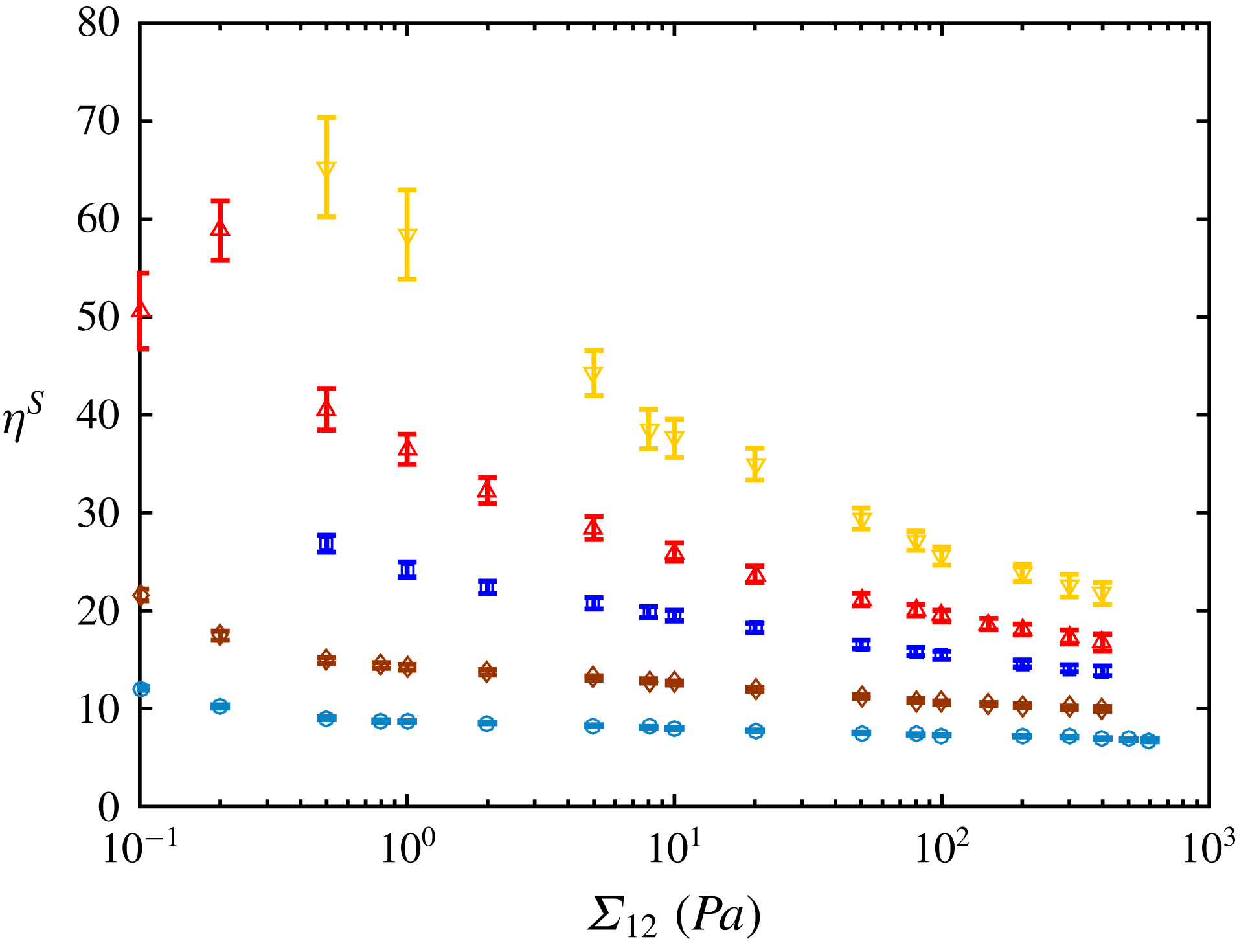
Figure 15 displays the shear rate dependence of the relative viscosity,
 $\unicode[STIX]{x1D702}_{S}=\unicode[STIX]{x1D702}/\unicode[STIX]{x1D702}_{0}$
, corrected using the Mooney–Rabinovitch correction (4.2) for the five particle volume fractions: 0.4, 0.43, 0.45, 0.47 and 0.49. The measurement uncertainties have been estimated by reloading five times the suspensions in the rheometer.
Relative viscosity as a function of shear stress. Symbols:
 $40~\unicode[STIX]{x03BC}\text{m}$
PS particles; (○)
 $\unicode[STIX]{x1D719}=0.4$
, (♢)
 $\unicode[STIX]{x1D719}=0.43$
, (▫)
 $\unicode[STIX]{x1D719}=0.45$
, (▵)
 $\unicode[STIX]{x1D719}=0.47$
, (▿)
 $\unicode[STIX]{x1D719}=0.49$
.

The shear-thinning behaviour extends over a range of more than the three decades that have been tested and is more pronounced as the particle volume fraction increases. These results are very consistent with those of Tanner & Dai (Reference Tanner and Dai2016) obtained with the same particles (Microbeads, TS40) dispersed in a silicon oil (viscosity 1.1 Pa s) in a slightly narrower range of shear stress.
5 Discussion: comparison between experiments and simulations
No simulations were performed for
 $\unicode[STIX]{x1D719}=0.43$
and
 $\unicode[STIX]{x1D719}=0.49$
. However, since the model defined in (3.3) accurately fits the simulation data, the experimental data are compared to the model. In addition, in order to draw the experimental and numerical data on the same figure, a single value of the critical stress
 $\unicode[STIX]{x1D6F4}_{c}$
has to be stated for all values of the volume fraction so that
 $\unicode[STIX]{x1D702}^{S}\dot{\unicode[STIX]{x1D6E4}}=\unicode[STIX]{x1D6F4}_{12}/\unicode[STIX]{x1D6F4}_{c}$
. We determine the value that fits the best is
 $\unicode[STIX]{x1D6F4}_{c}=9.53$
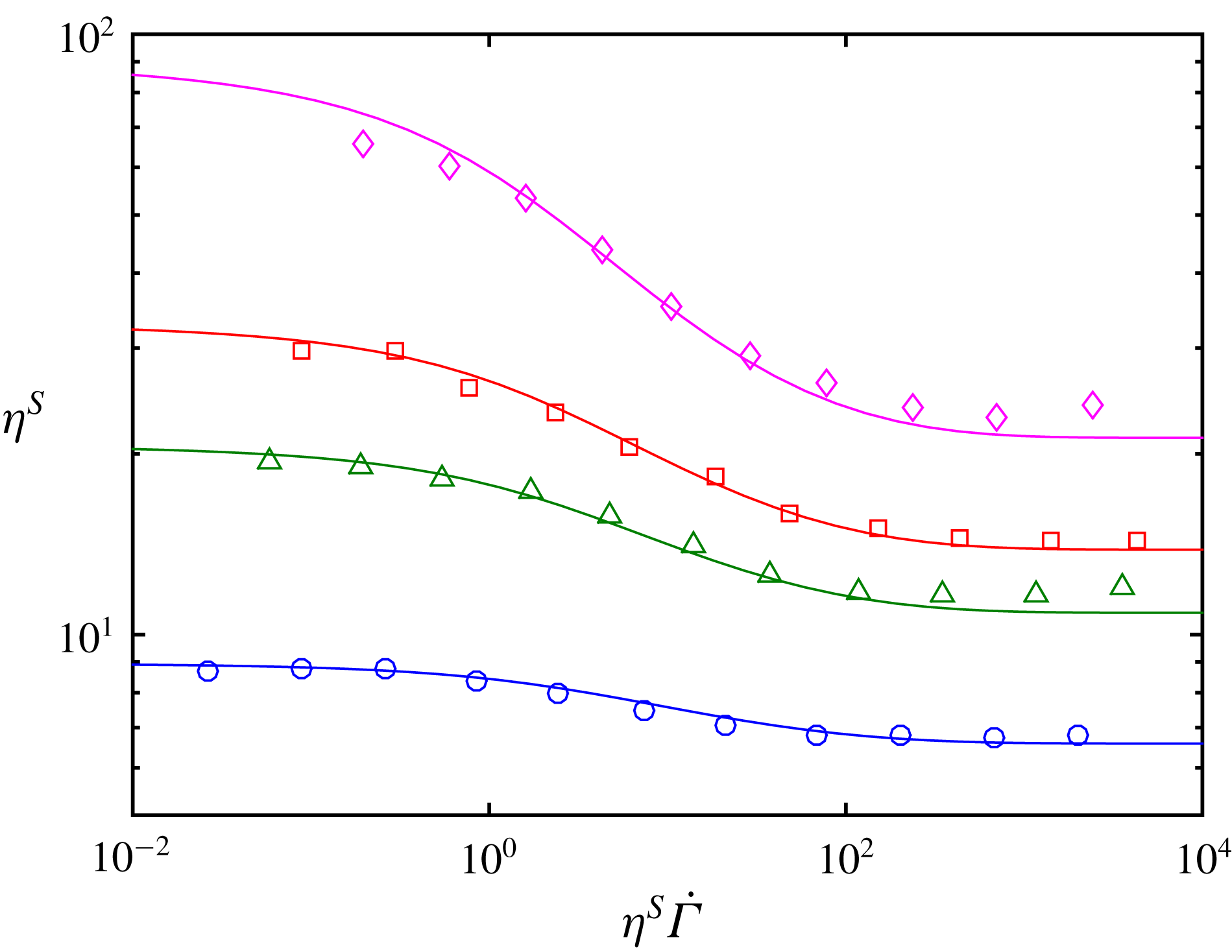
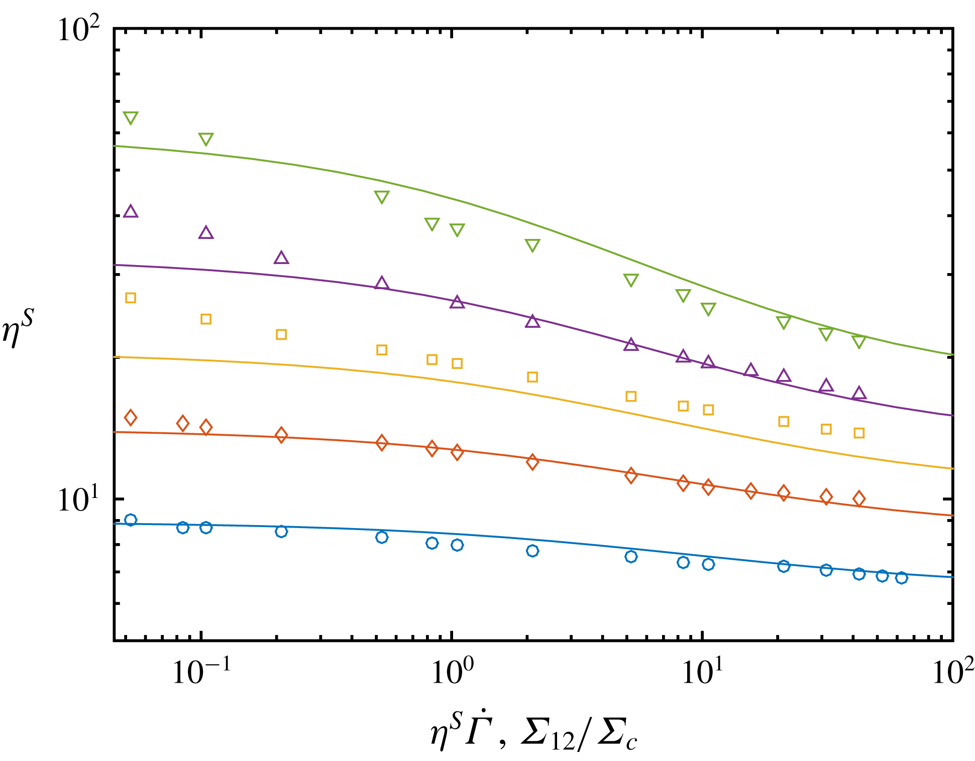
Pa. Figure 16 displays the suspension viscosity as a function of reduced shear stress, both experiments and model.
Viscosity as a function of reduced shear stress.
 $\unicode[STIX]{x1D719}=0.4$
,
 $\unicode[STIX]{x1D719}=0.43$
,
 $\unicode[STIX]{x1D719}=0.45$
,
 $\unicode[STIX]{x1D719}=0.47$
,
 $\unicode[STIX]{x1D719}=0.49$
. Symbols: experiments. Solid lines: model (3.3).

The experimental data are in quite good qualitative agreement with the model. The viscosity range for a given volume fraction is roughly the same in both cases, and spans the same reduced stress range too. From the value of the fitted critical stress
 $\unicode[STIX]{x1D6F4}_{c}=9.53$
Pa, we can deduce the value of the critical load
 $L_{c}$
:
 $L_{c}=\unicode[STIX]{x1D6F4}_{c}\times (6\unicode[STIX]{x03C0}a_{1}^{2})=46$
nN. As for the radius
 $a_{1}$
, this is
 $0.8$
times the mean radius of the bidisperse suspension in the simulations; we take
 $a_{1}=16~\unicode[STIX]{x03BC}\text{m}$
. The value of
 $L_{c}$
yields an estimation of the asperity radius of curvature
 $R_{exp}$
–
 $h_{r}$
in the contact law – using (2.4) together with the material constant in table 1:
 $R_{exp}\approx$
156 nm. We recall here that in the contact model, the asperity was considered as half a sphere of radius
 $h_{r}$
. However, the typical extension of an asperity in the direction parallel to the surface
 $L_{\Vert }$
may be different from the asperity height
 $h_{r}\sim 36~\text{nm}$
. This extension may be estimated from the curvature:
 $L_{\Vert }\sim \sqrt{2R_{exp}h_{r}}\approx 3.4~\unicode[STIX]{x03BC}\text{m}$
. We did not perform an extensive study of the surface roughness statistics. However, this value for the extension of an asperity is quite consistent with the AFM image displayed in figure 14. We note also that contact may occur through a few contact points instead of a single point as assumed in the model. The consequence would be qualitatively the same as increasing the radius of curvature, i.e. to increase the critical load. For instance, if the contact is supposed to involve two asperities, the curvature radius can be computed from
 $L_{c}=1/2\times \unicode[STIX]{x1D6F4}_{c}\times (6\unicode[STIX]{x03C0}a_{1}^{2})$
together with (2.4):
 $R_{exp}\approx 156/\sqrt{2}\approx$
110 nm, closer to
 $h_{r}$
. On the whole, this qualitative agreement suggests that the physical mechanism of the shear-thinning behaviour is satisfactorily captured by the load-dependent friction model.
In more detail, the viscosity from the model (or the simulations) presents some discrepancies with the experimental values. At low shear stress, the experimental viscosity does not really show any plateau, contrarily to what is expected from the model or the simulations. This difference may be explained by residual adhesion between particles regardless the great care that has been taken in the choice and in the preparation of the suspensions. Such adhesive interactions, even very small, should influence the viscosity at small enough shear stress. In the high stress range, the experimental measurement could not be performed at such high stresses that the viscosity plateau would be reached, due to the usual edge fracture in the parallel-plate geometry.
To go further in the comparison between the model and the experiments, it is possible to compute for each stress the parameters of the viscosity model
 $\unicode[STIX]{x1D6FC}_{0}(\unicode[STIX]{x1D6F4}_{12})$
and
 $\unicode[STIX]{x1D719}_{m}(\unicode[STIX]{x1D6F4}_{12})$
from the experimental data. These experimental parameters are displayed in figures 12 and 13, respectively, against the reduced shear stress, together with their numerical counterparts. We chose the same value of the critical stress
 $\unicode[STIX]{x1D6F4}_{c}=9.53$
Pa as in figure 16. The variations of
 $\unicode[STIX]{x1D719}_{m}$
from the experiments and from the model are in quite good agreement, with approximately the same volume fraction range, and the same reduced stress range. However, the experimental jamming fraction takes one value under
 $\unicode[STIX]{x1D719}_{m}^{\infty }$
at low shear stress, possibly due to the residual adhesion mentioned above. The experimental and numerical data for
 $\unicode[STIX]{x1D6FC}_{0}$
are in quite good agreement too, even though the experimental values are above those of the model. It should be stressed here that the values of
 $\unicode[STIX]{x1D6FC}_{0}$
and
 $\unicode[STIX]{x1D719}_{m}$
from the experiment significantly depend on the precise adjustment procedure, apparently due to the dispersion of the experimental data, especially in the low stress range, where the discrepancies are larger. It does not affect the qualitative shape of the
 $\unicode[STIX]{x1D719}_{m}$
curve, but leads to variations of
 $\unicode[STIX]{x0394}\unicode[STIX]{x1D719}_{m}\sim 0.01$
.
Finally the effective friction coefficient
 $\unicode[STIX]{x1D707}^{eff}(\unicode[STIX]{x1D6F4}_{12})$
can be computed from the experimental jamming volume fraction (figure 13) reversing (3.2). It is then assumed, as previously in (3.4), that
 $\unicode[STIX]{x1D707}^{eff}$
is actually the microscopic friction coefficient for the applied load
 $\bar{F}_{n}=6\unicode[STIX]{x03C0}a_{1}^{2}\unicode[STIX]{x1D6F4}_{12}/1.69$
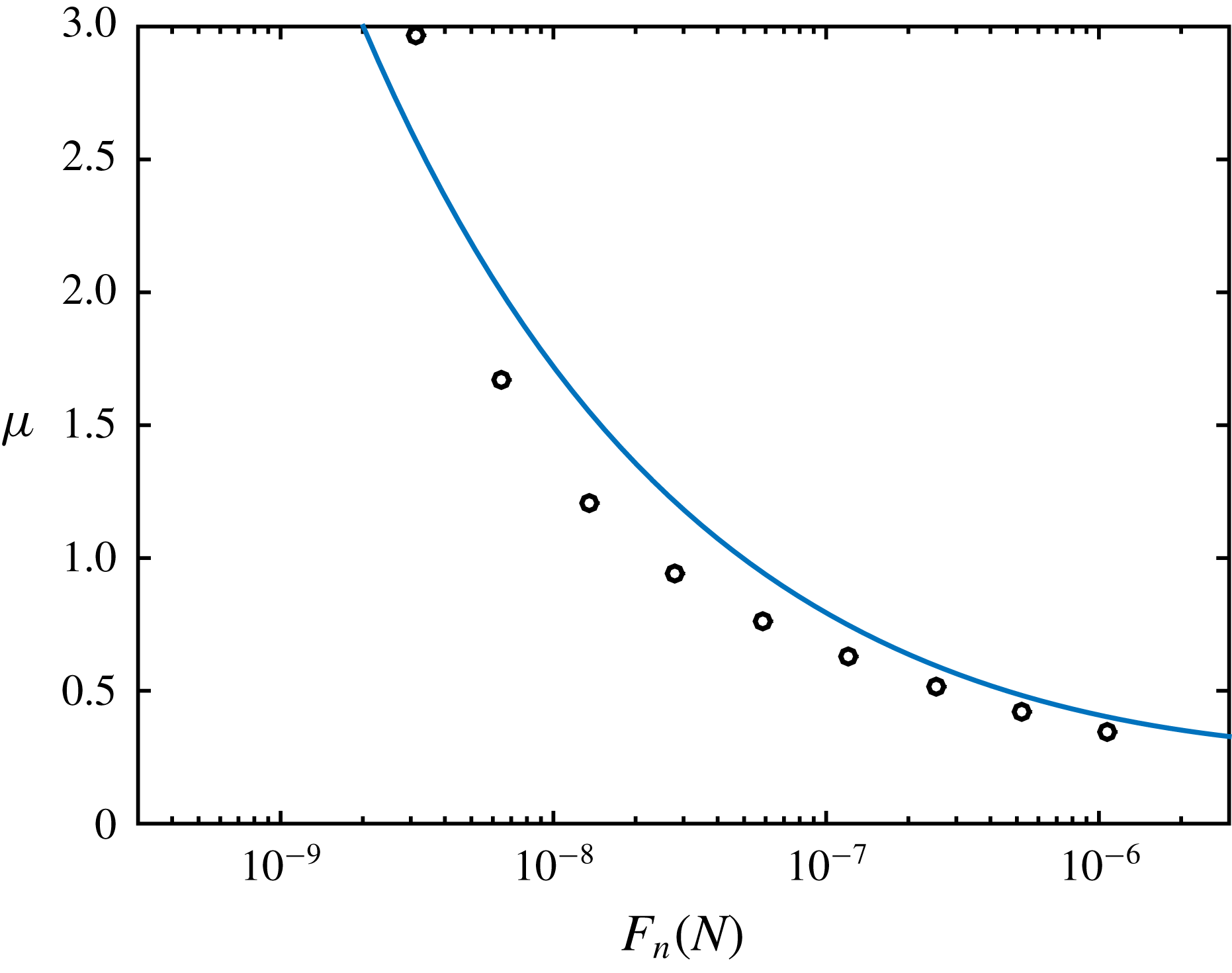
. The variation of resulting experimental load-dependent friction coefficient with the normal load is displayed in figure 17, together with the mono-asperity contact model (3.3). As expected, the experimental data are in quite satisfactory agreement with the mono-asperity contact model. We note that it is possible to deduce
 $\unicode[STIX]{x1D707}^{eff}$
from the viscosity measurements only if the values of the experimental jamming fraction belong to the variation range of
 $\unicode[STIX]{x1D719}_{m}$
deduced from the numerical simulations at constant friction coefficient. These values are between
 $\unicode[STIX]{x1D719}_{m}^{\infty }=0.546$
for
 $\unicode[STIX]{x1D707}\rightarrow \infty$
and
 $\unicode[STIX]{x1D719}_{m}^{0}=0.70$
for
 $\unicode[STIX]{x1D707}=0$
. Thus the inversion procedure presented above can be used only for values of the force corresponding to values of
 $\unicode[STIX]{x1D719}_{m}$
larger than the minimum value
 $\unicode[STIX]{x1D719}_{m}^{\infty }$
, i.e.
 $F_{n}>3$
nN. The values of the friction coefficient deduced from the viscosity measurements must be considered an estimation rather than a precise quantification. As shown in figure 6, for
 $\unicode[STIX]{x1D707}\gtrsim 2$
,
 $\unicode[STIX]{x1D719}_{m}$
hardly varies with
 $\unicode[STIX]{x1D707}$
so that even a low error on
 $\unicode[STIX]{x1D719}_{m}$
may have a significant impact on the value of
 $\unicode[STIX]{x1D707}$
.
Microscopic friction coefficient. Symbol: experimental data. Solid line: mono-asperity model from (3.4) with
 $L_{c}=46$
nN.

6 Conclusion
In this paper it is shown that it is possible to capture the shear-thinning behaviour that is observed in most concentrated non-Brownian frictional suspensions by considering variable friction interactions between particles. Owing to the low interparticle forces involved in sheared suspensions, it is expected that particles come into contact through one or a few asperities. For such a contact, it is anticipated that the value of the friction coefficient varies with normal load and thus with shear stress. To test the effect of variable friction on suspension rheology, we introduce in a numerical simulation code based on the force coupling method, a contact law adapted from the numerical work of Brizmer et al. (Reference Brizmer, Kligerman and Etsion2007). This model considers an elastic–plastic contact and results in a decrease of the friction coefficient at low normal loads followed by its saturation at high normal loads. The results of the simulations show a decrease of the viscosity with the shear stress that is in the same range as that observed experimentally. The comparison between simulations conducted either with constant friction coefficient or load-dependent friction coefficient makes it possible to propose a model for the shear-thinning viscosity. As already shown by Peters et al. (Reference Peters, Ghigliotti, Gallier, Blanc, Lemaire and Lobry2016) and Singh et al. (Reference Singh, Mari, Denn and Morris2018), the viscosity in the former case (constant friction coefficient) increases with the friction coefficient, mainly due to the decrease of the jamming volume fraction. In the proposed viscosity model for the particles with load-dependent friction coefficient, the effective friction coefficient
 $\unicode[STIX]{x1D707}^{eff}$
is specified by the effective normal contact force which is simply proportional to the shear stress. As the shear stress increases,
 $\unicode[STIX]{x1D707}^{eff}$
decreases and the jamming volume fraction increases, leading to the reduction of the viscosity. A very good agreement between the model and the simulations is found. These results are compared to experimental measurements carried out on suspensions of polystyrene particles (
 $40~\unicode[STIX]{x03BC}\text{m}$
in diameter) dispersed in silicone oil for five particle volume fractions between 0.40 and 0.49. The overall agreement between the model (or the simulations) and the experiments is satisfactory. The viscosity reduction as the shear stress increases is well captured by the model and the variation of the jamming volume fraction with the shear stress from the experiments is in quite good agreement with the predictions. The closeness between the experiments and the predictions of the model enabled us to evaluate the friction coefficient and its variation with the applied shear stress from rheometric measurements. Finally, the simplistic nature of the contact law deserves a few words. The essential feature is the variation of the friction coefficient with load, that is connected to the small number of asperities in contact – here a single asperity – in contrast to the usual model of a statistical distribution of contacting asperities. Such a mono-asperity contact model could be refined at will, to take into account a finite number of asperities, possibly growing with the bore load. This may also have an influence on the way the friction coefficient levels off at large load, possibly supplementing or even replacing plasticity. More generally, due to the complexity of contact at microscopic scale, and to the number of parameters that are potentially relevant in the surface physical chemistry, the next step to gaining a more quantitative understanding of the physical mechanism leading to this shear-thinning behaviour would be to determine the friction law between particles from colloidal probe AFM measurements.
Acknowledgements
The authors thank C. Claudet and O. Volkova for the AFM roughness measurements. This work was granted access to the HPC and visualisation resources of the Centre de Calcul Interactif hosted by Université Nice Sophia Antipolis.
Appendix A. Normal stress differences
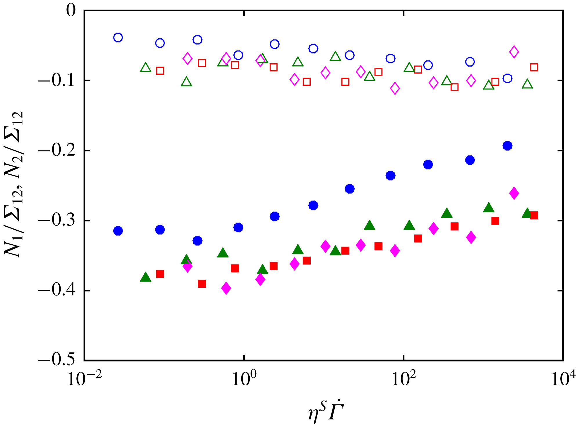
Figure 18 presents the variation of the two normal stress differences normalised by the shear stress,
 $N_{1}/\unicode[STIX]{x1D6F4}_{12}$
and
 $N_{2}/\unicode[STIX]{x1D6F4}_{12}$
, with the non-dimensional stress
 $\unicode[STIX]{x1D702}^{S}\dot{\unicode[STIX]{x1D6E4}}$
. These results are consistent with previous numerical results performed with a constant friction coefficient and present the same characteristics (Gallier et al.
Reference Gallier, Lemaire, Peters and Lobry2014): both
 $N_{1}$
and
 $N_{2}$
are negative,
 $N_{1}$
is much smaller than
 $N_{2}$
. The values of the reduced normal stress differences are also of the same order of magnitude as those obtained with a friction coefficient in the range [0.3–0.5]. At last,
 $N_{2}/\unicode[STIX]{x1D6F4}_{12}$
appears not to vary much with
 $\unicode[STIX]{x1D719}$
for
 $\unicode[STIX]{x1D719}\geqslant 0.45$
. This saturation of
 $N_{2}/\unicode[STIX]{x1D6F4}_{12}$
has already been observed in experiments (Zarraga et al.
Reference Zarraga, Hill and Leighton2000; Boyer, Pouliquen & Guazzelli Reference Boyer, Pouliquen and Guazzelli2011; Dbouk, Lobry & Lemaire Reference Dbouk, Lobry and Lemaire2013) and in numerical simulations conducted at constant friction coefficient (Gallier et al.
Reference Gallier, Lemaire, Peters and Lobry2014). Concerning the variation of
 $N_{1}/\unicode[STIX]{x1D6F4}_{12}$
and
 $N_{2}/\unicode[STIX]{x1D6F4}_{12}$
with
 $\unicode[STIX]{x1D702}^{S}\dot{\unicode[STIX]{x1D6E4}}$
, the trends are also consistent with the numerical results that have been obtained with different constant friction coefficients. According to the findings of §§ 3.2 and 3.3, increasing
 $\unicode[STIX]{x1D702}^{S}\dot{\unicode[STIX]{x1D6E4}}$
leads to a decrease of the friction coefficient. Figure 18 shows that the magnitude of
 $N_{1}/\unicode[STIX]{x1D6F4}_{12}$
increases and that of
 $N_{2}/\unicode[STIX]{x1D6F4}_{12}$
decreases with increasing
 $\unicode[STIX]{x1D702}^{S}\dot{\unicode[STIX]{x1D6E4}}$
, just as the magnitude of
 $N_{1}/\unicode[STIX]{x1D6F4}_{12}$
increases and that of
 $N_{2}/\unicode[STIX]{x1D6F4}_{12}$
decreases when the friction coefficient decreases, as shown by Gallier et al. (Reference Gallier, Lemaire, Peters and Lobry2014).
Open symbols: reduced first normal stress difference. Closed symbols: reduced second normal stress difference. (○)
 $\unicode[STIX]{x1D719}=40\,\%$
, (▵)
 $\unicode[STIX]{x1D719}=45\,\%$
, (▫)
 $\unicode[STIX]{x1D719}=47\,\%$
, (♢)
 $\unicode[STIX]{x1D719}=50\,\%$
.

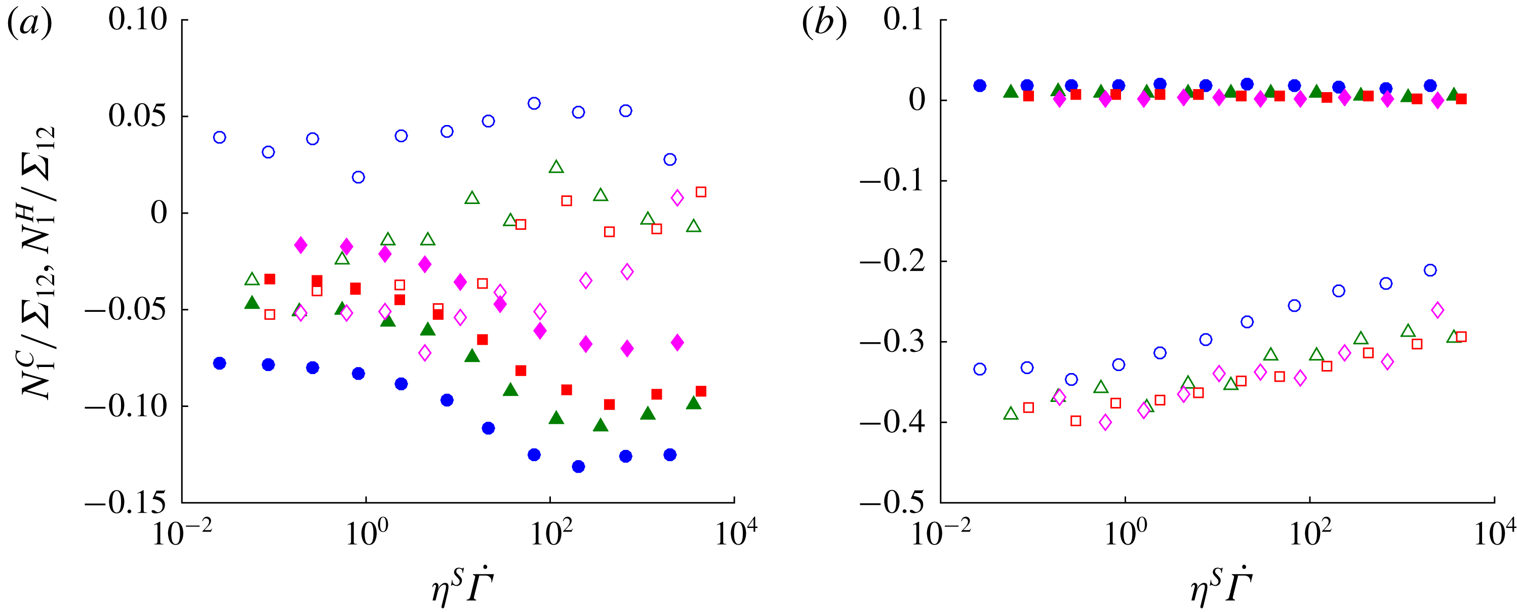
The hydrodynamic and contact contributions to the normal stress differences are displayed in figure 19. It is difficult to compare the trends displayed in figure 19(a) with the results of Gallier et al. (Reference Gallier, Lemaire, Peters and Lobry2014). The latter seem to indicate that for particle volume fractions larger than 0.4,
 $N_{1}^{H}/\unicode[STIX]{x1D6F4}_{12}$
hardly varies with
 $\unicode[STIX]{x1D707}$
while the magnitude of
 $N_{1}^{C}/\unicode[STIX]{x1D6F4}_{12}$
tends to decrease weakly with increasing
 $\unicode[STIX]{x1D707}$
. The behaviour of the shear-thinning suspensions considered here seems to be different, with a trend of decreasing
 $N_{1}^{H}/\unicode[STIX]{x1D6F4}_{12}$
and of increasing
 $N_{1}^{C}/\unicode[STIX]{x1D6F4}_{12}$
with increasing
 $\unicode[STIX]{x1D702}^{S}\dot{\unicode[STIX]{x1D6E4}}$
. But we have to keep in mind that both
 $N_{1}^{H}$
and
 $N_{1}^{C}$
are much smaller than the total stresses,
 $\unicode[STIX]{x1D6F4}_{11}$
and
 $\unicode[STIX]{x1D6F4}_{22}$
, from which they are deduced and can be very sensitive to the details of the suspension microstructure that may be a little different from a non-shear-thinning suspension. Concerning the results obtained for
 $N_{2}^{H}$
and
 $N_{2}^{C}$
, they are consistent with those of Gallier et al. (Reference Gallier, Lemaire, Peters and Lobry2014) with a small
 $N_{2}^{H}$
compared to
 $N_{2}^{C}$
and a trend of
 $N_{2}^{C}$
decreasing in magnitude with increasing
 $\unicode[STIX]{x1D702}^{S}\dot{\unicode[STIX]{x1D6E4}}$
.
(a) Reduced first normal stress difference. (b) Reduced second normal stress difference. Open symbols: contact contribution. Closed symbols: hydrodynamic contribution. Same volume fractions as in figure 18.

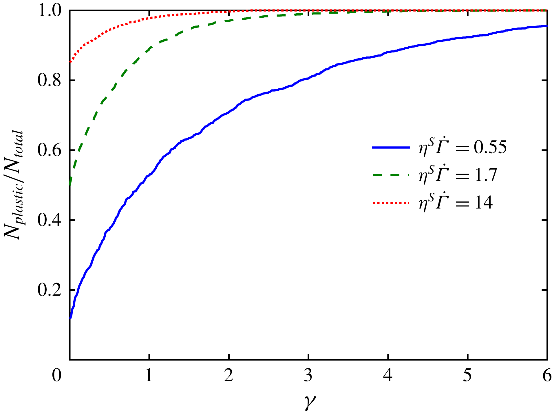
Variation of the fraction of particles that have experienced a plastic contact as a function of strain time for three values of
 $\unicode[STIX]{x1D702}^{S}\dot{\unicode[STIX]{x1D6E4}}$
at
 $\unicode[STIX]{x1D719}=0.45$
.

Appendix B. Some elements on contact statistics
Figure 20 displays the fraction of particles that have experienced plastic contact versus strain for three values of
 $\unicode[STIX]{x1D702}^{S}\dot{\unicode[STIX]{x1D6E4}}$
at
 $\unicode[STIX]{x1D719}=0.45$
. The initial value of
 $N_{Plastic}/N_{Total}$
is the average fraction of particles that undergo plastic contact. As the strain increases,
 $N_{Plastic}/N_{Total}$
increases with an exponential-like relaxation. From this variation, we deduce a characteristic strain
 $\unicode[STIX]{x1D6FE}_{c}$
which is the average strain necessary for a particle to undergo a plastic contact. The variation of
 $\unicode[STIX]{x1D6FE}_{c}$
with
 $\unicode[STIX]{x1D702}^{S}\dot{\unicode[STIX]{x1D6E4}}$
is displayed in figure 21 for the four values of the particle volume fraction. As
 $\unicode[STIX]{x1D702}^{S}\dot{\unicode[STIX]{x1D6E4}}$
increases,
 $\unicode[STIX]{x1D6FE}_{c}$
decreases and reaches for
 $\unicode[STIX]{x1D702}^{S}\dot{\unicode[STIX]{x1D6E4}}\approx 1$
a plateau whose value depends on the volume fraction. A qualitative understanding is quite straightforward. For reduced stress
 $\unicode[STIX]{x1D702}^{S}\dot{\unicode[STIX]{x1D6E4}}$
smaller than
 $2\times 10^{-1}$
no particle was found to undergo plastic deformation. As the reduced stress increases, the probability of a plastic contact takes a finite value, leading to a high value of the characteristic strain that decreases as the probability of plastic contact increases. For reduced stress larger that typically one, the characteristic strain levels off to a plateau. We note significant noise for the largest value of the reduced stress. The strain range of the simulation may be too short to reach completely satisfying statistical accuracy.
Characteristic strain for a particle to undergo a plastic contact.

Fraction of plastic contacts
 $f_{F_{n}>L_{c}}$
as a function of reduced shear stress. Same volume fractions as in figure 6.

A deeper understanding can be achieved by plotting the fraction of plastic contacts
 $f(F_{N}>L_{c})$
against
 $\unicode[STIX]{x1D702}^{S}\dot{\unicode[STIX]{x1D6E4}}$
. As shown in figure 22, the data obtained for the four particle volume fractions collapse on a single curve. Figure 22 is very similar to what has been obtained by Mari et al. (Reference Mari, Seto, Morris and Denn2014) who studied the fraction of frictional contacts in a shear-thickening suspension. They showed that the number of contacts was controlled by a competition between the applied shear forces and the short-range repulsive forces between particles. It is quite remarkable that similar results on contact statistics are obtained for discontinuous shear-thickening and shear-thinning suspensions, these two cases being different in many respects. In particular, in the description of discontinuous shear-thickening proposed by Mari et al. (Reference Mari, Seto, Morris and Denn2014), the repulsive force between particles controls the transition from a frictionless (
 $\unicode[STIX]{x1D707}=0$
) rheology to a contact dominated (
 $\unicode[STIX]{x1D707}\approx 1$
) rheology. In contrast, in the model of shear thinning that we propose here, the characteristic plastic force
 $L_{c}$
marks a soft transition from high to low friction coefficient that is continuously crossed by the sheared suspension.