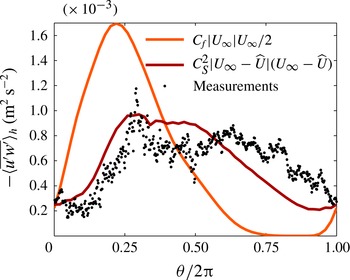
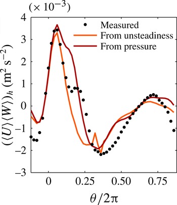
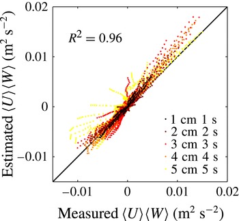
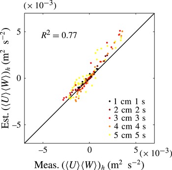
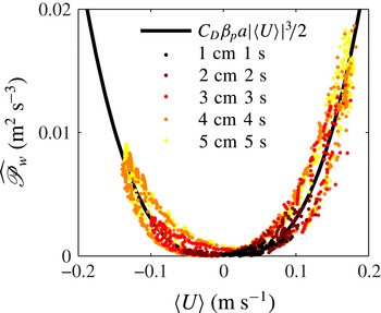
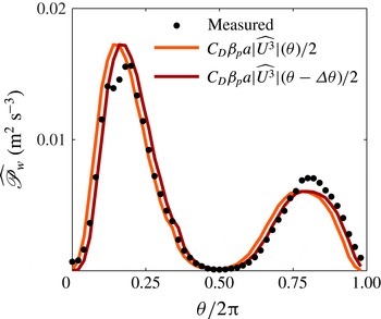
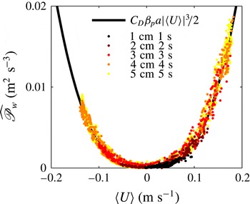
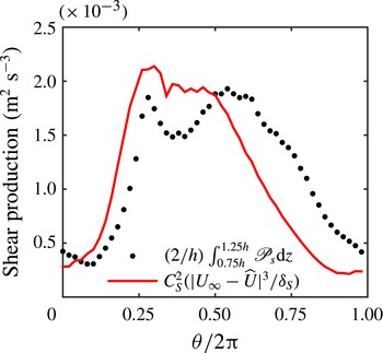
1. Introduction
Submerged aquatic canopies, such as coral reefs and seagrass meadows, play an important role in controlling physical and biological processes in aquatic ecosystems, including wave attenuation, nutrient cycling and sediment transport (Ward, Kemp & Boynton Reference Ward, Kemp and Boynton1984; López & García Reference López and García1998; Falter, Atkinson & Merrifield Reference Falter, Atkinson and Merrifield2004; Lowe et al. Reference Lowe, Falter, Koseff, Monismith and Atkinson2007; Bradley & Houser Reference Bradley and Houser2009; Taebi et al. Reference Taebi, Lowe, Pattiaratchi, Ivey, Symonds and Brinkman2011). Modelling of flow through these systems is critical to coastal and estuarine management and to understanding how ecosystems will react to a changing climate (Orth et al. Reference Orth, Carruthers, Dennison, Duarte, Fourqurean, Heck, Hughes, Kendrick, Kenworthy, Olyarnik, Short, Waycott and Williams2006; Monismith Reference Monismith2007; Waycott et al. Reference Waycott, Duarte, Carruthers, Orth, Dennison, Olyarnik, Calladine, Fourqurean, Heck, Hughes, Kendrick, Kenworthy, Short and Williams2009).
Canopy flow has been studied extensively, beginning with unidirectional flow over terrestrial canopies, such as cities and forests. A review of this work is provided in Finnigan (Reference Finnigan2000). The terrestrial canopy flow literature provided the initial framework for studying aquatic canopies and similarities have been found over a range of scales and applications (Ghisalberti Reference Ghisalberti2009). More recently, oscillatory canopy flow has been a growing area of research (Lowe et al. Reference Lowe, Shavit, Falter, Koseff and Monismith2008; Bradley & Houser Reference Bradley and Houser2009; Luhar et al. Reference Luhar, Coutu, Infantes, Fox and Nepf2010; Pujol & Nepf Reference Pujol and Nepf2012; Weitzman et al. Reference Weitzman, Aveni-Deforge, Koseff and Thomas2013). Wave-driven flows are common in coastal ecosystems and their dynamics differ significantly from the dynamics of unidirectional flow (Lowe, Koseff & Monismith Reference Lowe, Koseff and Monismith2005). Wave forcing is often the dominant driver of processes of interest in coastal systems, such as sediment resuspension, nutrient uptake and biomechanical failure (Storlazzi et al. Reference Storlazzi, Brown, Field, Rodgers and Jokiel2005; Hansen & Reidenbach Reference Hansen and Reidenbach2011; Weitzman et al. Reference Weitzman, Aveni-Deforge, Koseff and Thomas2013). Thus, practical models for wave-driven canopy flow are required for a variety of applications, from ecosystem conservation to coastal protection.
While this work was motivated by coral reefs and seagrass meadows, insights from oscillatory aquatic canopy flow may be relevant to a variety of applications. In terrestrial canopy flows, complex terrain and eddies from the atmospheric boundary layer could both induce spatially or temporally unsteady features (Calaf, Meneveau & Meyers Reference Calaf, Meneveau and Meyers2010; Belcher, Harman & Finnigan Reference Belcher, Harman and Finnigan2012). However, these are difficult to mimic experimentally and computationally expensive to simulate. Wave-driven aquatic flows provide a convenient test bed for studying unsteady turbulence dynamics in canopies. The periodicity facilitates ensemble averaging and the scales are reasonable to mimic in the laboratory. Understanding of wave-driven unsteadiness in coral reefs may provide insights that help in designing vertical-axis wind turbine arrays or predicting the dispersal of urban pollutants (Whittlesey, Liska & Dabiri Reference Whittlesey, Liska and Dabiri2010; Philips, Rossi & Iaccarino Reference Philips, Rossi and Iaccarino2013).
1.1. Aquatic canopy flow modelling
Many models have been developed to better understand the physics of flow through submerged aquatic canopies. These tend to be in one of two categories: models that capture bulk quantities and are extremely simple, and models that attempt to capture complex dynamics and are computationally expensive or difficult to implement. Lowe et al. (Reference Lowe, Koseff and Monismith2005) developed a simple 2-box model for estimating the depth-averaged in-canopy velocity from the freestream velocity in oscillatory flow and Luhar et al. (Reference Luhar, Coutu, Infantes, Fox and Nepf2010) used the 2-box model to show that pure oscillatory flow induces a mean current within a flexible canopy. Lowe et al. (Reference Lowe, Shavit, Falter, Koseff and Monismith2008) then further developed the 2-box model by comparing it with porous media flow theory. More complex models include those of King, Tinoco & Cowen (Reference King, Tinoco and Cowen2012), who developed a one-dimensional (1D)
 $k{-}{\it\epsilon}$
model for unidirectional canopy flow; Li & Yan (Reference Li and Yan2007), who developed a three-dimensional (3D) 1-equation eddy viscosity model for wave–current interaction with vegetation; and Maza, Lara & Losada (Reference Maza, Lara and Losada2013), who developed a two-dimensional (2D)
 $k{-}{\it\epsilon}$
model coupled with a vegetation dynamics model for wave-driven flow in flexible canopies. All three of these models include complex parameterizations for the effects of wake scale turbulence on the large scale momentum transfer, which are difficult to verify.
In this study, a 0-equation Reynolds-averaged Navier–Stokes (RANS) model was developed for predicting velocity profiles in combined wave–current canopy flows. The model was designed to balance simplicity and accuracy to make it widely applicable in field and laboratory studies, as well as large scale numerical models. To accommodate different use cases, the model has flexible resolution. At minimum resolution, it can act as a 2-box model, which is primarily useful for estimating the depth-averaged in-canopy velocity. Alternatively, the resolution can be increased to compute a well-resolved velocity profile. To reflect this flexibility, the model will be referred to as an N-box model.
While the idea of an N-box model is fairly obvious, there are two reasons why this type of model is not yet widely used: it is difficult to validate and it is not clear that it would be accurate. Accurate accounting of the unsteady momentum budget requires Reynolds-averaged and volume-averaged statistics, which are typically very difficult to measure. Ensemble averaging by wave phase requires extremely precise synchronization between the waves and the measurements because turbulent fluctuations represent a very weak signal compared with the wave-induced velocities. In the field, this type of synchronization is exceptionally difficult, and in the laboratory it requires that the wave actuation and the measurements are controlled by the same hardware. In light of these obstacles, most studies of wavy canopy flow settle for measurements of time-averaged statistics, such as root-mean-squared (r.m.s.) velocities (Lowe et al. Reference Lowe, Koseff and Monismith2005; Luhar et al. Reference Luhar, Coutu, Infantes, Fox and Nepf2010; Hansen & Reidenbach Reference Hansen and Reidenbach2011; Stevens & Lacy Reference Stevens and Lacy2012; Luhar et al. Reference Luhar, Infantes, Orfila, Terrados and Nepf2013). Although r.m.s. statistics quantify the magnitude of flow variability, they do not allow computation of the unsteady momentum budget terms. Lowe et al. (Reference Lowe, Shavit, Falter, Koseff and Monismith2008) captured the measurements required for direct ensemble-averaging by wave phase, but did not present phase-dependent turbulence statistics or a phase-dependent momentum budget.
Volume-averaging requires high-resolution in-canopy measurements over a region that is representative of the entire in-canopy space. Because canopy elements act as barriers to physical and optical access, most studies have to use sparse in-canopy measurements and assume that these are representative of the volume average (Lowe et al. Reference Lowe, Koseff and Monismith2005, Reference Lowe, Shavit, Falter, Koseff and Monismith2008; Hu et al. Reference Hu, Suzuki, Zitman, Uittewaal and Stive2014). It is also common practice to remove elements and take measurements in the gap, which is not necessarily representative of the in-canopy space (Neumeier & Ciavola Reference Neumeier and Ciavola2004; Luhar et al. Reference Luhar, Coutu, Infantes, Fox and Nepf2010; King et al. Reference King, Tinoco and Cowen2012; Pujol et al. Reference Pujol, Serra, Colomer and Casamitjana2013). Without unsteady Reynolds averaging and true volume averaging, the system dynamics are under-resolved and parameterizations are difficult to verify.
It is typically assumed that the Reynolds stress is a dominant term in the momentum budget and that improving model accuracy requires more complex turbulence modelling. This then suggests that a simple N-box model would be inaccurate and 1- or 2-equation turbulence models that account for canopy-scale and wake-scale turbulence are required, as in Li & Yan (Reference Li and Yan2007). Contrary to this, recent laboratory studies have suggested that in oscillatory flow, the Reynolds stress is only significant in extreme cases (Lowe et al. Reference Lowe, Shavit, Falter, Koseff and Monismith2008; Ghisalberti & Schlosser Reference Ghisalberti and Schlosser2013). Proper validation of this idea requires phase-dependent Reynolds stress measurements, which were not presented by either study. If Reynolds stress is small, complex turbulence models are unnecessary, and an N-box model could represent a simple, powerful tool for wavy canopy flows.
To address these issues, experiments were conducted to measure statistics with true volume averaging and ensemble averaging by wave phase in combined wave–current canopy flows. These laboratory results were used as a platform for a deep exploration of canopy flow modelling.
-
(a) Parameterizations for terms in the momentum and turbulent kinetic energy (TKE) budgets were evaluated directly, rather than being validated through testing of a numerical model.
-
(b) A simple N-box model was developed and validated for predicting velocity profiles in combined wave–current flows. The model is easy to understand and computationally efficient because it uses a simple Reynolds stress parameterization.
-
(c) The relative importance of the in-canopy momentum budget terms was assessed analytically and tested experimentally. Over a significant portion of the parameter space relevant to combined wave–current canopy flows, the Reynolds stress is expected to be a small contributor, indicating that the N-box model would be an effective tool in this space.
1.2. The volume-averaged equations
Volume-averaged momentum and energy equations provide the basic framework for understanding canopy flows. According to the review by Finnigan (Reference Finnigan2000), the averaging volume
‘consists of a horizontal slab, extensive enough in the horizontal to eliminate plant-to-plant variations in canopy structure but thin enough to preserve the characteristic variation of properties in the vertical’.
The advantage of applying this filter is that it creates relationships between the large-scale flow structure and correlations that capture the effects of small-scale spatial heterogeneity and fluid–element interaction. By parameterizing these correlations in terms of volume-averaged quantities, the equations of motion can be greatly simplified.
Under the volume-averaging framework, scale separation between the horizontal and vertical flow structure can be leveraged to yield vertically 1D governing equations, essentially treating canopy flow as a thin shear layer. The canopy is assumed to be horizontally homogeneous and extensive enough in the streamwise and transverse directions that there exists a region within the canopy where edge effects do not cause significant horizontal gradients in the volume-averaged statistics. Wave transformation due to shoaling and attenuation is assumed to occur over large distances, so the associated streamwise gradients of time-averaged statistics are negligible. Far from the canopy edges, the waves are assumed to be the dominant source of streamwise variability and their wavelength is assumed to be large compared with the canopy height. Under these assumptions, a sampling region with a streamwise extent that is much smaller than the wavelength will have horizontally homogeneous volume-averaged statistics that only depend on the height above the bottom,
 $z$
, and the wave phase,
 ${\it\theta}$
. The streamwise gradients of velocity statistics can be neglected in the momentum budget. For the phase-dependent component of any volume-averaged statistic, the wave frequency,
 ${\it\omega}$
, and the wavenumber,
 $k_{w}$
, can be used to translate between gradients in phase, gradients in time and gradients in the streamwise direction,
 $\partial /\partial {\it\theta}=(1/{\it\omega})(\partial /\partial t)=(1/k_{w})(\partial /\partial x)$
. Because the waves are assumed to be the dominant source of streamwise variability, the phase-dependence of volume-averaged statistics is the dominant driver of streamwise gradients.
1.2.1. Momentum
The assumptions above lead to the following form of the volume-averaged streamwise momentum equation (Finnigan Reference Finnigan2000):
 $$\begin{eqnarray}\frac{\partial \!\left\langle U\right\rangle }{\partial t}+\frac{\partial \!\left(\left\langle U\right\rangle \left\langle W\right\rangle \right)}{\partial z}=-\frac{1}{{\it\rho}}\frac{\partial \!\left\langle P\right\rangle }{\partial x}+\frac{\partial {\it\tau}_{xz}}{\partial z}-F_{D}-F_{I}\end{eqnarray}$$
where
 $U$
and
 $W$
are the streamwise and vertical velocity, respectively,
 $P$
is the pressure,
 $F_{D}$
is the drag force and
 $F_{I}$
is the inertia force. Angle brackets denote volume-averaging. Capitals and overbars denote ensemble averaging by wave phase. The shear stress,
 ${\it\tau}_{xz}$
, is composed of three terms:
 $$\begin{eqnarray}{\it\tau}_{xz}=-\!\left\langle \overline{u^{\prime }w^{\prime }}\right\rangle -\left\langle U^{\prime \prime }W^{\prime \prime }\right\rangle +{\it\nu}\frac{\partial \left\langle U\right\rangle }{\partial z}\end{eqnarray}$$
where primes denote fluctuations about the ensemble average and double primes denote fluctuations about the volume average. The volume-averaged Reynolds stress,
 $\langle \overline{u^{\prime }w^{\prime }}\rangle$
, is typically assumed to be the dominant shear stress term, so
 ${\it\tau}_{xz}\approx -\langle \overline{u^{\prime }w^{\prime }}\rangle$
. The dispersive flux,
 $\langle U^{\prime \prime }W^{\prime \prime }\rangle$
, arises from spatial correlation of mean velocities. It is typical to assume that
 $\langle U^{\prime \prime }W^{\prime \prime }\rangle$
is negligible, an assertion that is rarely verified because
 $\langle U^{\prime \prime }W^{\prime \prime }\rangle$
is difficult to measure, but is supported by the experimental results of Moltchanov, Bohbot-Raviv & Shavit (Reference Moltchanov, Bohbot-Raviv and Shavit2011). The viscous stress,
 ${\it\nu}\partial \langle U\rangle /\partial z$
, is negligible at high Reynolds number. The system is forced by the pressure gradient, which can be due to a time-average free-surface slope or surface waves. In order to solve the momentum equation,
 $\langle W\rangle$
,
 ${\it\tau}_{xz}$
,
 $F_{D}$
and
 $F_{I}$
must be estimated from
 $\langle U\rangle$
.
A common practice is to break the water column into two ‘boxes’ and consider the momentum budget in the lower box (Lowe et al. Reference Lowe, Koseff and Monismith2005). To do this, the streamwise momentum budget is averaged over the in-canopy space, ignoring the vertical advection and Reynolds stress at the bottom boundary:
 $$\begin{eqnarray}\frac{\partial \widehat{U}}{\partial t}+\frac{\left[\left\langle U\right\rangle \left\langle W\right\rangle \right]_{h}}{h}=-\frac{1}{{\it\rho}}\frac{\partial \widehat{P}}{\partial x}+\frac{\left.{\it\tau}_{xz}\right|_{h}}{h}-\widehat{F}_{D}-\widehat{F}_{I}\end{eqnarray}$$
where the hat is used to denote in-canopy depth-averaged quantities.
1.2.2. Turbulent kinetic energy
The volume-averaged TKE budget can be written as follows:
 $$\begin{eqnarray}\frac{\partial \!\left\langle k\right\rangle }{\partial t}+\left\langle W\right\rangle \frac{\partial \!\left\langle k\right\rangle }{\partial z}=\mathscr{P}_{s}+\mathscr{P}_{w}+\frac{\partial T_{k}}{\partial z}-\left\langle {\it\epsilon}\right\rangle\end{eqnarray}$$
where
 $k$
is the TKE,
 $T_{k}$
is the transport of TKE and
 ${\it\epsilon}$
is the dissipation of TKE. The shear production,
 $\mathscr{P}_{s}$
, and the wake production,
 $\mathscr{P}_{w}$
, represent the two components of turbulence production that arise from volume averaging:
 $$\begin{eqnarray}\displaystyle & \displaystyle \mathscr{P}_{s}=-\!\left\langle \overline{u^{\prime }w^{\prime }}\right\rangle \frac{\partial \!\left\langle U\right\rangle }{\partial z} & \displaystyle\end{eqnarray}$$
 $$\begin{eqnarray}\displaystyle & \displaystyle \mathscr{P}_{w}\approx -\!\left\langle \overline{u^{\prime 2}}^{\prime \prime }\frac{\partial U^{\prime \prime }}{\partial x}\right\rangle -\left\langle \overline{u^{\prime }v^{\prime }}^{\prime \prime }\left(\frac{\partial U^{\prime \prime }}{\partial y}+\frac{\partial V^{\prime \prime }}{\partial x}\right)\right\rangle -\left\langle \overline{v^{\prime 2}}^{\prime \prime }\frac{\partial V^{\prime \prime }}{\partial y}\right\rangle & \displaystyle\end{eqnarray}$$
 $\mathscr{P}_{s}$
and
 $\mathscr{P}_{w}$
represent two different mechanisms by which turbulence is produced. Here
 $\mathscr{P}_{s}$
results from large-scale vertical gradients and generates turbulence primarily above the top of the canopy. In contrast,
 $\mathscr{P}_{w}$
results from small-scale horizontal gradients caused by element drag and generates turbulence within the canopy. Estimates of
 $\mathscr{P}_{s}$
and
 $\mathscr{P}_{w}$
are necessary for computing a TKE budget and, because of the differences in the two mechanisms, they are important for understanding the properties of the turbulence generated in canopy flows.
1.3. Parameterizations
A variety of canopy flow parameterizations were evaluated in this study. Parameterizations for drag, Reynolds stress and vertical advection were evaluated for use in the momentum budget (1.1) and parameterizations for
 $\mathscr{P}_{w}$
and
 $\mathscr{P}_{s}$
were evaluated because of their relevance to canopy turbulence. The inertia force is also included in this section, although it was not tested for reasons that will become clear in a later section.
In order to simplify notation, three important velocities are defined. The freestream velocity,
 $U_{\infty }$
, is the depth-averaged velocity above the canopy:
 $$\begin{eqnarray}U_{\infty }=\frac{1}{H-h}\int _{h}^{H}\left\langle U\right\rangle \!\text{d}z\end{eqnarray}$$
where
 $h$
is the canopy height and
 $H$
is the depth. The current velocity,
 $U_{c}$
, is the time average of the freestream velocity:
 $$\begin{eqnarray}U_{c}=\frac{1}{2{\rm\pi}}\int _{0}^{2{\rm\pi}}U_{\infty }\text{d}{\it\theta}.\end{eqnarray}$$
The wave velocity,
 $U_{w}$
, is the r.m.s. of the phase-dependent portion of the freestream velocity:
 $$\begin{eqnarray}U_{w}=\sqrt{\frac{1}{2{\rm\pi}}\int _{0}^{2{\rm\pi}}\left(U_{\infty }-U_{c}\right)^{2}\text{d}{\it\theta}}.\end{eqnarray}$$
In order to use ‘freestream’ velocities to parameterize the flow, the canopy is assumed to be under shallow submergence, but far from emergent, so
 $2<H/h<5$
. This regime is relevant for many natural aquatic canopies (Nepf Reference Nepf2012).
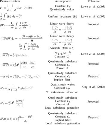
The remainder of this section provides a brief introduction to the parameterizations and their underlying assumptions. A summary is provided in table 1.
Summary of parameterizations.

1.3.1. Drag force
The drag force exerted by the canopy is typically parameterized with a quadratic drag law with a constant
 $C_{D}$
(Lowe et al.
Reference Lowe, Koseff and Monismith2005; King et al.
Reference King, Tinoco and Cowen2012).
 $$\begin{eqnarray}F_{D}=\frac{1}{2}\frac{1}{1-{\it\phi}}C_{D}a\left|\left\langle U\right\rangle \right|\left\langle U\right\rangle\end{eqnarray}$$
where
 $a$
is the canopy’s frontal area per unit volume and
 ${\it\phi}$
is the volume fraction of the canopy (King et al.
Reference King, Tinoco and Cowen2012). In the present study
 ${\it\phi}$
is generally assumed to be small enough that it can be neglected. The underlying assumptions for the quadratic drag parameterization are that the wakes are quasi-steady, the flow around the elements is 2D, and the wakes do not interact with downstream elements.
In a 2-box model, another assumption is required in order to estimate the drag from the depth-averaged velocity. The simplest assumption is that
 $\langle U\rangle$
is uniform with depth inside the canopy (Lowe et al.
Reference Lowe, Koseff and Monismith2005):
 $$\begin{eqnarray}\frac{1}{h}\int _{0}^{h}\left\langle U\right\rangle ^{2}\text{d}z=\widehat{U}^{2}.\end{eqnarray}$$
The error associated with this parameterization increases as the vertical variability of
 $\langle U\rangle$
increases.
1.3.2. Vertical advection
In previous studies, vertical advection has been included in 2D and 3D models by numerically solving the pressure Poisson equation (Li & Yan Reference Li and Yan2007). This approach is computationally expensive and cannot be applied in 1D models. A simpler and more efficient approach is to parameterize the vertical advection using linear wave theory. The continuity equation
 $$\begin{eqnarray}\frac{\partial \!\left\langle W\right\rangle }{\partial z}=-\frac{\partial \!\left\langle U\right\rangle }{\partial x}\end{eqnarray}$$
can be depth-integrated to give the vertical velocity at the top of the canopy:
 $$\begin{eqnarray}\left\langle W\right\rangle =-\int _{0}^{z}\frac{\partial \!\left\langle U\right\rangle }{\partial x}\text{d}{\check{z}}.\end{eqnarray}$$
This can be related to the unsteadiness using the phase speed of the wave.
 $$\begin{eqnarray}\left\langle W\right\rangle =-\frac{k_{w}}{{\it\omega}}\int _{0}^{z}\frac{\partial \!\left\langle U\right\rangle }{\partial t}\text{d}{\check{z}}.\end{eqnarray}$$
Assuming that the pressure gradient and unsteadiness are in approximate balance gives an estimate of the vertical velocity at any
 $z$
-location in the water column
 $$\begin{eqnarray}\left\langle W\right\rangle =-\frac{k_{w}}{{\it\omega}}\int _{0}^{z}\frac{1}{{\it\rho}}\frac{\partial \!\left\langle P\right\rangle }{\partial x}\text{d}{\check{z}}.\end{eqnarray}$$
Multiplying this by
 $\langle U\rangle$
gives an estimate of the momentum flux due to vertical advection.
At low resolution, the spatial discretization can also be an important source of error. For finite-volume models, fluxes are computed at the box faces, so
 $\langle U\rangle$
is interpolated from the nodes. For example, in a 2-box model, there is a box face located at the canopy height. The momentum flux at the canopy height is computed by estimating
 $\langle W\rangle$
from (1.15) and interpolating
 $\langle U\rangle$
from
 $\widehat{U}$
and
 $U_{\infty }$
:
 $$\begin{eqnarray}\left[\left\langle U\right\rangle \left\langle W\right\rangle \right]_{h}=-\frac{\left(H-h\right)\widehat{U}+hU_{\infty }}{H}\frac{k_{w}}{{\it\omega}}\int _{0}^{h}\frac{1}{{\it\rho}}\frac{\partial \!\left\langle P\right\rangle }{\partial x}\text{d}z.\end{eqnarray}$$
When appropriate, the estimate can be further simplified by assuming shallow water waves:
 $$\begin{eqnarray}\left[\left\langle U\right\rangle \left\langle W\right\rangle \right]_{h}=-\frac{\left(H-h\right)\widehat{U}+hU_{\infty }}{H}\frac{h}{{\it\rho}\sqrt{gH}}\frac{\partial \!\left\langle P\right\rangle }{\partial x}.\end{eqnarray}$$
1.3.3. Reynolds stress
In the 2-box model presented by Lowe et al. (Reference Lowe, Koseff and Monismith2005), the momentum transfer between the two boxes is estimated from the above-canopy velocity and a friction coefficient,
 $C_{f}$
:
 $$\begin{eqnarray}-\!\left\langle \overline{u^{\prime }w^{\prime }}\right\rangle ={\textstyle \frac{1}{2}}C_{f}\left|U_{\infty }\right|U_{\infty }.\end{eqnarray}$$
This estimate is a quadratic friction type parameterization where the canopy is treated as bed roughness and the in-canopy velocity is assumed to be negligible. The
 $C_{f}$
parameterization is accurate for a canopy exposed to a steady current because the flow is fully developed and
 $\widehat{U}$
is typically small relative to
 $U_{\infty }$
(Lowe et al.
Reference Lowe, Koseff and Monismith2005). However, the parameterization may be less accurate in waves because
 $\widehat{U}$
is similar to
 $U_{\infty }$
.
To address the non-negligible
 $\widehat{U}$
and to accommodate higher-resolution models, the shear can be used to parameterize the Reynolds stress using the Smagorinsky model (Vreman, Geurts & Kuerten Reference Vreman, Geurts and Kuerten1997):
 $$\begin{eqnarray}-\!\left\langle \overline{u^{\prime }w^{\prime }}\right\rangle =C_{S}^{2}{\it\Delta}^{2}\left|\frac{\partial \!\left\langle U\right\rangle }{\partial z}\right|\frac{\partial \!\left\langle U\right\rangle }{\partial z}\end{eqnarray}$$
where
 $C_{S}$
is the Smagorinsky constant and
 ${\it\Delta}$
is the filter length. Typical values of
 $C_{S}$
fall between 1 and 2, with a canonical value of 1.7 (Vreman et al.
Reference Vreman, Geurts and Kuerten1997). If
 ${\it\Delta}$
is assumed to be equal to the length of the spatial discretization,
 ${\rm\Delta}z$
, it is referred to as an implicit filter. Applying the Smagorinsky model with an implicit filter to the 2-box model yields a relationship between the Reynolds stress and the velocity deficit:
 $$\begin{eqnarray}-\!\left\langle \overline{u^{\prime }w^{\prime }}\right\rangle _{h}=C_{S}^{2}|U_{\infty }-\widehat{U}|(U_{\infty }-\widehat{U}).\end{eqnarray}$$
1.3.4. Inertia force
The parameterization for the inertia force is
 $$\begin{eqnarray}F_{I}=\frac{C_{M}{\it\phi}}{1-{\it\phi}}\frac{\partial \!\left\langle U\right\rangle }{\partial t}\end{eqnarray}$$
where
 $C_{M}$
is the inertia force coefficient (Lowe et al.
Reference Lowe, Koseff and Monismith2005). In the context of the 2-box model, this can simply be adjusted to use the depth-averaged velocity. The inertia force can be neglected when
 ${\it\phi}$
is small. For this reason, it is generally ignored in this study.
1.3.5. Wake production
If all of the work done by drag is converted into TKE, then
 $\mathscr{P}_{w}=F_{D}\langle U\rangle$
. To account for direct conversion of mean flow kinetic energy into heat by viscosity, the factor
 ${\it\beta}_{p}$
is added (King et al.
Reference King, Tinoco and Cowen2012). Substituting the quadratic drag parameterization for
 $F_{D}$
results in a cubic relationship:
 $$\begin{eqnarray}\mathscr{P}_{w}=\frac{1}{2}\frac{1}{1-{\it\phi}}C_{D}{\it\beta}_{p}a\left|\left\langle U\right\rangle \right|^{3}\end{eqnarray}$$
where
 ${\it\phi}$
can be neglected when the volume fraction of the canopy is small, as in the present study. Because it is based on the drag, the
 $\mathscr{P}_{w}$
parameterization depends on the same assumptions that the drag parameterization is based on. Unsteadiness, 3D wake effects and heterogeneity in
 $U$
could all contribute to error. The appropriateness of
 ${\it\beta}_{p}$
is an additional assumption, which has yet to be validated with direct measurements of
 $\mathscr{P}_{w}$
.
1.3.6. Shear production
The Smagorinsky model for predicting
 $\langle \overline{u^{\prime }w^{\prime }}\rangle$
can be extended to estimate
 $\mathscr{P}_{s}$
:
 $$\begin{eqnarray}\mathscr{P}_{s}=C_{S}^{2}{\it\Delta}^{2}\left|\frac{\partial \!\left\langle U\right\rangle }{\partial z}\right|^{3}.\end{eqnarray}$$
Applying this to a 2-box model and assuming an implicit filter gives an estimate of
 $\mathscr{P}_{s}$
at the top of the canopy:
 $$\begin{eqnarray}\mathscr{P}_{s}\left(z=h\right)=C_{S}^{2}\frac{|U_{\infty }-\widehat{U}|^{3}}{{\it\delta}_{S}}\end{eqnarray}$$
where
 ${\it\delta}_{S}$
is some length scale for the discretization of the shear. Based on the locations of the box nodes,
 $H/2$
may be a logical choice for
 ${\it\delta}_{S}$
. However, in the submergence regime under consideration, the mixing layer growth is limited by the bottom boundary. Therefore, the distance over which
 $U_{\infty }$
transitions to
 $\widehat{U}$
is likely to be more closely related to
 $h$
. Thus, it may be stated more generally that
 $\mathscr{P}_{s}\sim |U_{\infty }-\widehat{U}|^{3}/h$
.
1.4.
 $N$
-box model

The framework of the 2-box model can easily be extended to an arbitrary number of boxes in order to predict velocity profiles. This results in a 1D finite-volume 0-equation unsteady RANS model. Such a model is desirable for a variety of reasons:
-
(a) the model is simple and computationally efficient;
-
(b) the resolution can be adjusted from 2 boxes to an arbitrary
$N$
boxes; -
(c) the model can easily be incorporated into a larger-scale ocean model.

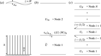
To derive an N-box model, the volume-averaged momentum equation is averaged over discrete boxes. The streamwise velocities are defined at the nodes. The vertical advection and the Reynolds stress are written in flux form and the fluxes are defined at the box faces:
 $$\begin{eqnarray}\frac{\partial U_{i}}{\partial t}=-\frac{\left[WU+{\it\tau}_{xz}\right]_{i+(1/2)}-\left[WU+{\it\tau}_{xz}\right]_{i-(1/2)}}{{\rm\Delta}z}-\left.\frac{1}{{\it\rho}}\frac{\partial P}{\partial x}\right|_{i}-{F_{D}}_{i}.\end{eqnarray}$$
Here, the
 $i$
subscript is used to denote the average over the
 $i$
th box. A schematic of the spatial discretization is provided in figure 1. The pressure gradient is an input to the model and the other terms are estimated using the parameterizations described in § 1.3. The resulting system of first-order ordinary differential equations (ODEs) can be solved with a standard ODE solver.
Schematic of (a) wave-driven flow over a submerged rigid canopy, (b) the spatial discretization for the 2-box model and (c) the spatial discretization of the N-box model. Fluxes are defined at the box faces and streamwise velocity is defined at the nodes.

1.5. Scaling
It is important to consider where in parameter space the N-box model is expected to be effective. The Smagorinsky model is a relatively simple parameterization and is most appropriate when the Reynolds stress is small and therefore unlikely to be the dominant source of error.
In wave-exposed canopies, the balance between unsteadiness and the wave-driven pressure gradient is modulated by vertical advection, Reynolds stress, drag and the inertia force (see (1.1)). Canopy flows take time to develop and in oscillatory flow the dominant force balance depends on how much the flow is able to develop over each wave period. In cases where the flow does not have time to develop at all, the drag does not significantly reduce the in-canopy velocity, shear does not develop at the top of the canopy and the Reynolds stress is unable to develop. In cases where the development time and the wave period are comparable, the drag becomes significant. In extreme cases where the wave period is very large compared with the development time, the drag greatly reduces the in-canopy velocity, shear develops at the top of the canopy and the Reynolds stress can become significant.
The spectrum from short wave periods to long wave periods relative to development time was discussed by Lowe et al. (Reference Lowe, Koseff and Monismith2005). However, little emphasis has been placed on the transitional region where drag can play an important role but the Reynolds stress is still relatively small. This region deserves further study for two reasons. First, it may encompass a large portion of the parameter space that is relevant to natural aquatic canopies. Second, if the drag is much larger than the Reynolds stress, a simple, standard turbulence model, such as the Smagorinsky parameterization, is appropriate because the drag parameterization is likely to be a more significant source of error. This has important implications because the Reynolds stress parameterization tends to be the primary driver of model complexity and computational cost. Furthermore, if the drag is the dominant source of error, improvements to the drag parameterization may be the best way to improve the accuracy of canopy flow models.
In the sections that follow, the region of applicability of the N-box model is identified through scaling similar to that in Lowe et al. (Reference Lowe, Koseff and Monismith2005). First, the non-dimensional momentum budget in the pure wave case is derived and analysed. Then, the in-canopy velocity reduction in the pure current case is considered. Finally, the findings are used to estimate the relative scales of the momentum budget terms in the combined wave–current case.
1.5.1. Pure wave case
The depth-averaged in-canopy momentum budget (1.3) with the Smagorinsky, quadratic drag and inertia force parameterizations is as follows:
 $$\begin{eqnarray}\frac{\partial \widehat{U}}{\partial t}+\frac{\left[\left\langle U\right\rangle \left\langle W\right\rangle \right]_{h}}{h}=-\frac{1}{{\it\rho}}\frac{\partial \widehat{P}}{\partial x}+\frac{C_{S}^{2}}{h}\left|U_{\infty }-\widehat{U}\right|\left(U_{\infty }-\widehat{U}\right)-\frac{C_{D}a}{2(1-{\it\phi})}\left|\widehat{U}\right|\widehat{U}-\frac{C_{M}{\it\phi}}{1-{\it\phi}}\frac{\partial \widehat{U}}{\partial t}.\end{eqnarray}$$
The in-canopy and freestream velocities are non-dimensionalized by the wave-induced velocity:
 $$\begin{eqnarray}U_{\infty }^{\ast }=\frac{U_{\infty }}{U_{w}},\quad \widehat{U}^{\ast }=\frac{\widehat{U}}{U_{w}}.\end{eqnarray}$$
Time is non-dimensionalized by the inverse of the angular wave frequency,
 ${\it\omega}$
, which is the dominant time scale.
 $$\begin{eqnarray}t^{\ast }={\it\omega}t.\end{eqnarray}$$
In order to non-dimensionalize the vertical advection,
 $[\langle U\rangle \langle W\rangle ]_{h}$
, a scale for the vertical velocity at the top of the canopy can be derived from (1.14). This is done by assuming that the phase speed is the shallow water wave speed, substituting in the scale for the unsteadiness and integrating to the top of the canopy:
 $$\begin{eqnarray}\left\langle W\right\rangle \left(z=h\right)\sim \frac{h{\it\omega}U_{w}}{\sqrt{gH}}\end{eqnarray}$$
where
 $g$
is gravitational acceleration. The scale for the streamwise velocity at the top of the canopy is
 $U_{w}$
, which gives rise to the following non-dimensionalization:
 $$\begin{eqnarray}[\left\langle U\right\rangle \left\langle W\right\rangle ]_{h}^{\ast }=\frac{[\left\langle U\right\rangle \left\langle W\right\rangle ]_{h}}{\displaystyle \frac{1}{2}\frac{h{\it\omega}U_{w}^{2}}{\sqrt{gH}}}.\end{eqnarray}$$
The factor of
 $1/2$
is included because
 $\langle U\rangle$
and
 $\langle W\rangle$
are out of phase. According to linear wave theory, they are sinusoidal signals that are
 $90^{\circ }$
out of phase, which suggests that the amplitude of
 $\langle U\rangle \langle W\rangle$
is half the product of the amplitudes of
 $\langle U\rangle$
and
 $\langle W\rangle$
. The scale for the vertical advection includes the Froude number of the wave,
 $\mathit{Fr}_{w}$
, which is associated with nonlinearity:
 $$\begin{eqnarray}\mathit{Fr}_{w}=\frac{U_{w}}{\sqrt{gH}}\approx \frac{a_{w}}{H}\end{eqnarray}$$
where
 $a_{w}$
is the wave amplitude.
The pressure term is scaled using the hydrostatic pressure under the wave. According to linear wave theory, under the shallow water wave assumption, the wave amplitude is
 $U_{w}\sqrt{H/g}$
(Dalrymple & Dean Reference Dalrymple and Dean1991). Thus, the pressure gradient scales as the quotient between
 ${\it\rho}gU_{w}\sqrt{H/g}$
and the fluid density times the wavelength,
 ${\it\rho}\sqrt{gH}/{\it\omega}$
. This suggests that the pressure term is of the same scale as the unsteadiness and the following parameterization applies:
 $$\begin{eqnarray}\frac{\partial P^{\ast }}{\partial x^{\ast }}=\frac{1}{{\it\rho}{\it\omega}U_{w}}\frac{\partial P}{\partial x}.\end{eqnarray}$$
By substituting the non-dimensional terms defined above into the parameterized in-canopy depth-averaged momentum budget (1.26) and dividing both sides of the equation by the scale for the unsteadiness,
 ${\it\omega}U_{w}$
, the non-dimensional depth-averaged in-canopy momentum budget becomes the following:
 $$\begin{eqnarray}\displaystyle & & \displaystyle \frac{\partial \widehat{U}^{\ast }}{\partial t^{\ast }}+\frac{1}{2}\mathit{Fr}_{w}\left[\left\langle U\right\rangle \left\langle W\right\rangle \right]_{h}^{\ast }\nonumber\\ \displaystyle & & \displaystyle \quad =-\frac{\partial \widehat{P}^{\ast }}{\partial x^{\ast }}+\frac{A_{w}}{L_{S}}|U_{\infty }^{\ast }-\widehat{U}^{\ast }|(U_{\infty }^{\ast }-\widehat{U}^{\ast })-\frac{A_{w}}{L_{D}}|\widehat{U}^{\ast }|\widehat{U}^{\ast }-\frac{C_{M}{\it\phi}}{1-{\it\phi}}\frac{\partial \widehat{U}^{\ast }}{\partial t^{\ast }}.\end{eqnarray}$$
The scale factors for the Reynolds stress and the drag have been simplified using three additional length scales. The drag length scale
 $$\begin{eqnarray}L_{D}=\frac{2(1-{\it\phi})}{C_{D}a}\end{eqnarray}$$
and the shear length scale
 $$\begin{eqnarray}L_{S}=\frac{h}{C_{S}^{2}}\end{eqnarray}$$
are easily found in (1.26) and are length scales for the development of the drag and the Reynolds stress, respectively (Lowe et al. Reference Lowe, Koseff and Monismith2005). The orbital excursion of the wave
 $$\begin{eqnarray}A_{w}=\frac{U_{w}}{{\it\omega}}\end{eqnarray}$$
is a length scale of the wave based on the horizontal excursion of a particle according to linear wave theory (Lowe et al. Reference Lowe, Koseff and Monismith2005).
For the rest of this article, it will be assumed that
 ${\it\phi}\approx 0$
and therefore the inertia force is negligible. This is appropriate for the experiments in the present study and helps to clarify the analysis by removing the confounding effects of the inertia force. While it was not tested in this study, some of the trends described below may persist when
 ${\it\phi}\neq 0$
and the inertia force is significant.
In order to assess the scales of the Reynolds stress and the drag, it is important to consider the velocity reduction inside the canopy, which can be quantified by
 ${\it\alpha}$
(Lowe et al.
Reference Lowe, Koseff and Monismith2005):
 $$\begin{eqnarray}{\it\alpha}=\frac{\text{r.m.s.}\;(\widehat{U})}{\text{r.m.s.}\;(U_{\infty })}.\end{eqnarray}$$
The non-dimensional in-canopy velocity scales as
 $\widehat{U}^{\ast }\sim {\it\alpha}$
and the non-dimensional velocity deficit scales as
 $U_{\infty }^{\ast }-\widehat{U}^{\ast }\sim 1-{\it\alpha}$
. This gives scales for the drag and the Reynolds stress:
 $$\begin{eqnarray}\displaystyle & \displaystyle \text{drag}\sim \frac{A_{w}}{L_{D}}{\it\alpha}^{2} & \displaystyle\end{eqnarray}$$
 $$\begin{eqnarray}\displaystyle & \displaystyle \text{Reynolds stress}\sim \frac{A_{w}}{L_{S}}\left(1-{\it\alpha}\right)^{2}. & \displaystyle\end{eqnarray}$$
 ${\it\beta}$
, it becomes clear that their relative importance depends on
 $L_{D}/L_{S}$
and
 ${\it\alpha}$
:
 $$\begin{eqnarray}{\it\beta}=\frac{\text{r.m.s. (Reynolds stress)}}{\text{r.m.s. (drag)}}\sim \frac{L_{D}}{L_{S}}\frac{\left(1-{\it\alpha}\right)^{2}}{{\it\alpha}^{2}}.\end{eqnarray}$$
This quantitatively demonstrates relationships that are obvious from physical intuition. When the in-canopy flow is unattenuated (
 ${\it\alpha}\sim 1$
), drag dominates because there is no shear to support a Reynolds stress. When the in-canopy flow is greatly attenuated (
 ${\it\alpha}\ll 1$
), there is little flow available to produce drag and the strong shear can produce a large Reynolds stress. The flow attenuation is caused by the drag, so these two limiting cases occur when
 $A_{w}/L_{D}\rightarrow 0$
and
 $A_{w}/L_{D}\rightarrow \infty$
. In the former case,
 $A_{w}/L_{D}$
is a linear approximation for the velocity deficit because it is the cumulative drag over one wave period. Thus, when
 $A_{w}/L_{D}\ll 1$
, the following estimates apply:
 $$\begin{eqnarray}{\it\alpha}\sim 1-\frac{A_{w}}{L_{D}},\quad {\it\beta}\sim \frac{A_{w}}{L_{S}}.\end{eqnarray}$$
Based on (1.40), it is useful to consider the range of possible values for the drag to shear length ratio:
 $$\begin{eqnarray}\frac{L_{D}}{L_{S}}=\frac{2C_{S}^{2}(1-{\it\phi})}{C_{D}ah}.\end{eqnarray}$$
In order for a geometry to exhibit canopy behaviour, it must satisfy the requirement that
 $C_{D}ah>0.1$
(Ghisalberti Reference Ghisalberti2009). For
 $C_{S}$
in the range given by Vreman et al. (Reference Vreman, Geurts and Kuerten1997),
 $C_{S}^{2}\sim O(10^{-2})$
. Thus,
 $L_{D}/L_{S}\ll 1$
for any canopy geometry and
 ${\it\alpha}$
must be fairly small to generate a significant
 ${\it\beta}$
.
In order to put this limit on
 $L_{D}/L_{S}$
into context, aquatic canopies described in the literature tend to have
 $L_{D}/L_{S}\sim O(10^{-3}{-}10^{-1})$
. Canonical values of
 $C_{D}=1$
and
 $C_{S}=0.17$
can be used to estimate
 $L_{D}$
and
 $L_{S}$
for geometries observed in field studies. Based on this, the three species of coral measured in Reidenbach et al. (Reference Reidenbach, Koseff, Monismith, Steinbuck and Genin2006) had
 $L_{D}/L_{S}$
between 0.009 and 0.03. The seven species of branched coral measured by Marshall (Reference Marshall2000) had
 $L_{D}/L_{S}$
between 0.007 and 0.05. For canopies of seagrass,
 $L_{D}/L_{S}$
can be estimated by assuming that the grass stands up straight and rigid. For the geometries of the 10 species of seagrass reported in Luhar et al. (Reference Luhar, Coutu, Infantes, Fox and Nepf2010),
 $L_{D}/L_{S}$
varied between approximately 0.1 and 0.001, with typical values around 0.01.
Equation (1.40) can be used to estimate the ratio between the Reynolds stress and the drag for experiments in the literature. Based on the wavy cases in four studies (Lowe et al.
Reference Lowe, Koseff and Monismith2005, Reference Lowe, Shavit, Falter, Koseff and Monismith2008; Luhar et al.
Reference Luhar, Coutu, Infantes, Fox and Nepf2010; Pujol et al.
Reference Pujol, Serra, Colomer and Casamitjana2013), the largest estimated
 ${\it\beta}$
value was approximately 2 %, which comes from a case in Lowe et al. (Reference Lowe, Koseff and Monismith2005) where
 ${\it\alpha}=0.69$
and
 $L_{D}/L_{S}=0.095$
. More typical experimental values of
 ${\it\alpha}=0.85$
and
 $L_{D}/L_{S}=0.01$
suggest that
 ${\it\beta}=0.03\,\%$
is more typical.
One might argue that these experimental
 ${\it\beta}$
values are uncharacteristically small because it is difficult to generate large waves in the laboratory, but it can be shown that
 ${\it\beta}$
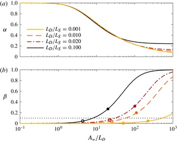
remains low even for fairly large waves over natural canopies. Following the approach of Lowe et al. (Reference Lowe, Koseff and Monismith2005), (1.33) was numerically integrated to compute
 ${\it\alpha}$
and
 ${\it\beta}$
in pure oscillatory flow over a wide range of
 $A_{w}/L_{D}$
(see figure 2). The value of
 ${\it\alpha}$
is independent of
 $L_{D}/L_{S}$
for
 $A_{w}/L_{D}$
up to 50 for all canopies and up to
 $A_{w}/L_{D}=200$
for typical canopies. This suggests that the in-canopy velocity is insensitive to the Reynolds stress over a large range of parameter space. Similar insensitivity to Reynolds stress was shown in Lowe et al. (Reference Lowe, Shavit, Falter, Koseff and Monismith2008).
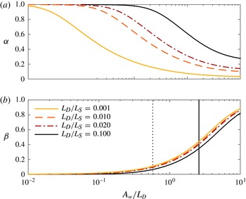
Plots of
 ${\it\alpha}$
and
 ${\it\beta}$
as a function of the orbital excursion to drag length ratio for four representative values of
 $L_{D}/L_{S}$
(see table 2). The curves are for the pure wave case and were generated by numerically integrating (1.33). The pressure gradient was assumed to be uniform throughout the water column and the inertia force and vertical advection were neglected with the intention of isolating the Reynolds stress and drag effects. Here
 ${\it\beta}$
was computed based on the r.m.s. Reynolds stress and drag. The open circles are for 10 s breaking waves at 1 m depth and the dots are for 20 s breaking waves at 5 m depth (see table 3). Smaller waves would be to the left on the
 ${\it\beta}$
curve.

Figure 2(b) demonstrates that
 $A_{w}/L_{D}$
has to be very large for the Reynolds stress to be significant compared with drag. At first inspection, it may seem that a canopy with large
 $L_{D}/L_{S}$
is more likely to have significant Reynolds stress. However, canopies with large
 $L_{D}/L_{S}$
logically have large values of
 $L_{D}$
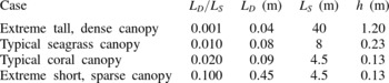
, indicating that they are sparse (see table 2). If
 $L_{D}$
is large, it takes much larger waves to produce large values of
 $A_{w}/L_{D}$
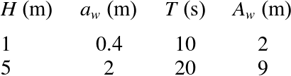
. To demonstrate this point, two extreme orbital excursions were chosen as reference points. These conditions are summarized in table 3 and the corresponding values of
 $A_{w}/L_{D}$
are indicated in figure 2. Only in the most extreme cases does
 ${\it\beta}$
become large. In fact, the results suggest that for all of the reference canopies, any wave with a period of 10 s or less in 1 m of water would produce a Reynolds stress that is less than 10 % of the drag.
Parameters for representative canopies. The
 $L_{D}/L_{S}$
and associated
 $L_{D}$
values were chosen to be representative of the values in Marshall (Reference Marshall2000), Reidenbach et al. (Reference Reidenbach, Koseff, Monismith, Steinbuck and Genin2006) and Luhar et al. (Reference Luhar, Coutu, Infantes, Fox and Nepf2010) with the assumption that
 $C_{D}=1$
and
 $C_{S}=0.17$
. The
 $L_{S}$
and
 $h$
values were computed from the other two quantities.

Conditions chosen for the reference extreme orbital excursions. In order to allow large waves, the
 $H$
values were chosen to be at the upper end of the specified submergence ratio range (
 $2<H/h<5$
) for very tall coral and seagrass canopy heights. The wave amplitudes were chosen to be at the breaking limit of
 $a_{w}/H=0.4$
(Dalrymple & Dean Reference Dalrymple and Dean1991). Based on linear wave theory, waves produce their most extreme orbital excursions when they are at their breaking limit. The wave period,
 $T$
, values were chosen to be in the middle and the upper end of the spectrum for swell waves. The orbital excursions were computed based on the other values according to linear wave theory.

Plots of
 ${\it\alpha}$
and
 ${\it\beta}$
as a function of the orbital excursion to shear length ratio for the four representative values of
 $L_{D}/L_{S}$
(see table 2). The curves are for the pure wave case and were generated by the same approach as figure 2. The vertical lines mark the extreme wave cases for the shortest canopies presented in the literature, which have
 $L_{S}=3.5~\text{m}$
based on
 $h=0.1$
m and
 $C_{S}=0.17$
. The dotted line is for the 10 s wave and the solid line is for the 20 s wave (see table 3).

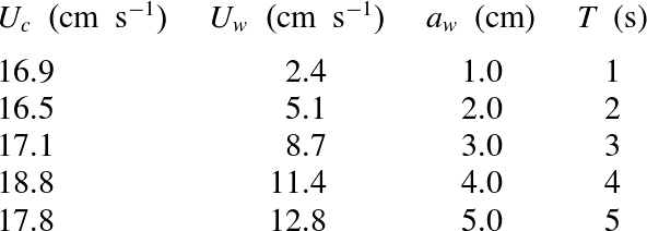
Parameters of the five flow conditions.

In order to remove the confounding dependence on
 $L_{D}$
, figure 3 demonstrates the dependence of
 ${\it\alpha}$
and
 ${\it\beta}$
on
 $A_{w}/L_{S}$
. Where
 ${\it\alpha}$
collapses as a function of
 $A_{w}/L_{D}$
because it is insensitive to Reynolds stress,
 ${\it\beta}$
collapses as a function of
 $A_{w}/L_{S}$
because it is insensitive to drag (this is consistent with (1.41)). In order to relate the collapsed
 ${\it\beta}$
curve to natural canopies,
 $h=10~\text{cm}$
was chosen as a lower bound for aquatic canopies based on all the observations in Marshall (Reference Marshall2000), Reidenbach et al. (Reference Reidenbach, Koseff, Monismith, Steinbuck and Genin2006), Lowe et al. (Reference Lowe, Shavit, Falter, Koseff and Monismith2008) and Luhar et al. (Reference Luhar, Coutu, Infantes, Fox and Nepf2010). The corresponding
 $A_{w}/L_{S}$
values for the reference extreme waves are marked in figure 3(b). Clearly, the Reynolds stress can become significant when the canopy is short and the waves are extremely large; an excellent example is provided by the artificial canopy flows in Ghisalberti & Schlosser (Reference Ghisalberti and Schlosser2013), which had
 $h=3~\text{cm}$
and
 $A_{w}$
up to 1.2 m. However,
 ${\it\beta}$
is small over a very large region of parameter space that is relevant to natural aquatic canopies in pure oscillatory flow.
To summarize, all canopy geometries have
 $L_{D}/L_{S}\ll 1$
. For pure wave cases with
 $A_{w}/L_{D}\ll 10$
, there is little velocity reduction within the canopy, so
 ${\it\alpha}\sim 1$
. Because
 $L_{D}/L_{S}$
is small and because large orbital excursions are required to generate a velocity deficit, it is only in the most extreme pure wave cases that the Reynolds stress becomes significant compared with drag.
1.5.2. Current-only case
In order to incorporate the effect of the background current in combined wave–current flows, the current-only case is first considered. In this case, (1.26) reduces to the following:
 $$\begin{eqnarray}0=-\frac{1}{{\it\rho}}\frac{\partial \widehat{P}}{\partial x}+\frac{1}{L_{S}}\left|U_{\infty }-\widehat{U}\right|\left(U_{\infty }-\widehat{U}\right)-\frac{1}{L_{D}}\left|\widehat{U}\right|\widehat{U}.\end{eqnarray}$$
The pressure gradient for unidirectional flow is uniform with depth and based on a depth-averaged momentum budget, the pressure balances the drag:
 $$\begin{eqnarray}-\frac{H}{{\it\rho}}\frac{\partial \widehat{P}}{\partial x}=\frac{h}{L_{D}}\left|\widehat{U}\right|\widehat{U}.\end{eqnarray}$$
Substituting for the pressure in (1.43) gives
 $$\begin{eqnarray}\frac{1}{L_{S}}\left|U_{\infty }-\widehat{U}\right|\left(U_{\infty }-\widehat{U}\right)=\left(1-\frac{h}{H}\right)\frac{1}{L_{D}}\left|\widehat{U}\right|\widehat{U}.\end{eqnarray}$$
Dividing both sides by
 $U_{\infty }$
and applying the scaling
 ${\it\alpha}_{c}\sim \widehat{U}/U_{\infty }$
,
 $$\begin{eqnarray}\frac{L_{D}}{L_{S}}(1-{\it\alpha}_{c})^{2}\sim \left(1-\frac{h}{H}\right){\it\alpha}_{c}^{2}.\end{eqnarray}$$
Solving for
 ${\it\alpha}_{c}$
gives the following:
 $$\begin{eqnarray}{\it\alpha}_{c}\sim \frac{\sqrt{\displaystyle \frac{L_{D}}{L_{S}}}}{\sqrt{\displaystyle \frac{L_{D}}{L_{S}}}+\sqrt{\displaystyle 1-\frac{h}{H}}}\end{eqnarray}$$
which reduces to
 $\sqrt{L_{D}/L_{S}}$
as in Lowe et al. (Reference Lowe, Koseff and Monismith2005) when
 $L_{D}/L_{S}\rightarrow 0$
and
 $h/H\rightarrow 0$
. For this study,
 $h/H$
is assumed to be between
 $1/2$
and
 $1/5$
and
 $L_{D}/L_{S}\ll 1$
. This indicates that
 ${\it\alpha}_{c}\ll 1$
. Thus, current-induced velocities are strongly attenuated by the canopy.
1.5.3. Combined waves and currents
The results of the analysis in §§ 1.5.1 and 1.5.2 can be used to develop scales for the momentum budget terms in the combined wave–current case. The following assumptions are made:
 $A_{w}/L_{D}\ll 10$
,
 $L_{D}/L_{S}\ll 1$
,
 $U_{c}/U_{w}\sim O(1)$
,
 $2<H/h<5$
and
 $\mathit{Fr}_{w}\ll 1$
. Based on the analysis of the pure wave case, when
 $A_{w}/L_{D}$
is small,
 ${\it\alpha}_{w}\approx 1$
. Based on the analysis of the pure current case, when
 $L_{D}/L_{S}$
is small,
 ${\it\alpha}_{c}\ll 1$
. Physically, this indicates that wave-induced velocities fully penetrate into the canopy, but the current is strongly attenuated inside the canopy. Although the two flows will not superpose linearly, it is assumed that these results still hold in the combined wave–current case. Because
 $U_{c}$
and
 $U_{w}$
are of the same order, the waves dominate the in-canopy velocity,
 $\widehat{U}\sim U_{w}$
, and the current dominates the velocity deficit,
 $U_{\infty }-\widehat{U}\sim U_{c}$
. With this finding, each of the momentum budget terms will now be scaled for the combined wave–current case.
The unsteadiness scales as
 ${\it\omega}U_{w}$
, just as in the pure wave case, so the entire momentum budget can be non-dimensionalized by
 ${\it\omega}U_{w}$
once again:
 $$\begin{eqnarray}\text{unsteadiness}\sim O(1).\end{eqnarray}$$
For the vertical advection, the pure wave scaling for the vertical velocity holds because the current does not induce vertical velocity. However, the velocity at the top of the canopy is from a combination of the waves and the current, and therefore scales as
 $\sqrt{U_{c}^{2}+U_{w}^{2}}$
. This gives a revised non-dimensionalization for the vertical advection:
 $$\begin{eqnarray}[\left\langle U\right\rangle \left\langle W\right\rangle ]_{h}^{\ast }=\frac{[\left\langle U\right\rangle \left\langle W\right\rangle ]_{h}}{\displaystyle \frac{1}{2}\frac{h{\it\omega}U_{w}}{\sqrt{gH}}\sqrt{U_{c}^{2}+U_{w}^{2}}}.\end{eqnarray}$$
It is convenient to define a Froude number for the combined wave–current velocity:
 $$\begin{eqnarray}\mathit{Fr}=\frac{\sqrt{U_{c}^{2}+U_{w}^{2}}}{\sqrt{gH}}.\end{eqnarray}$$
This gives the non-dimensional scale for the vertical advection:
 $$\begin{eqnarray}\text{vertical advection}\sim {\textstyle \frac{1}{2}}\mathit{Fr}.\end{eqnarray}$$
For the pressure gradient, the wave component is of the same order as the unsteadiness, as shown in the pure wave case. The mean component of the pressure gradient balances the current drag, as shown in the pure current case. Non-dimensionalizing the mean pressure gradient by
 ${\it\omega}U_{w}$
suggests the following:
 $$\begin{eqnarray}\left[\frac{\partial P^{\ast }}{\partial x^{\ast }}\right]_{c}\sim \frac{h}{H}\frac{{\it\alpha}_{c}^{2}U_{c}^{2}}{L_{D}}\frac{1}{{\it\omega}U_{w}}.\end{eqnarray}$$
Because
 $U_{c}\sim U_{w}$
, this can be rewritten as the following:
 $$\begin{eqnarray}\left[\frac{\partial P^{\ast }}{\partial x^{\ast }}\right]_{c}\sim \frac{h}{H}{\it\alpha}_{c}^{2}\frac{A_{w}}{L_{D}}.\end{eqnarray}$$
Based on our assumptions,
 $h/H$
is less than unity,
 $A_{w}/L_{D}\ll 10$
, and
 ${\it\alpha}_{c}\ll 1$
. Thus, the mean pressure gradient can be neglected and only the wave-induced pressure gradient remains:
 $$\begin{eqnarray}\text{pressure}\sim O(1).\end{eqnarray}$$
For the Reynolds stress, it is now clear that the velocity deficit scales with the mean current, so the Reynolds stress scale is adjusted for the combined wave–current case:
 $$\begin{eqnarray}\text{Reynolds stress}\sim \frac{A_{w}}{L_{S}}{U_{c}^{\ast }}^{2}\end{eqnarray}$$
where
 $U_{c}^{\ast }=U_{c}/U_{w}$
.
For the drag, the waves dominate the in-canopy velocity, so the scale from the pure wave case with
 ${\it\alpha}_{w}\approx 1$
is appropriate:
 $$\begin{eqnarray}\text{drag}\sim \frac{A_{w}}{L_{D}}.\end{eqnarray}$$
Based on the arguments and assumptions presented above, in the parameter space where
 $A_{w}/L_{D}\ll 10$
,
 $L_{D}/L_{S}\ll 1$
,
 $U_{c}/U_{w}\sim O(1)$
,
 $2<H/h<5$
and
 $\mathit{Fr}\ll 1$
, the hierarchy for the in-canopy momentum budget is expected to be the following:
 $$\begin{eqnarray}\displaystyle \text{pressure }\sim \text{unsteadiness }\gg \text{drag }\gg \text{advection},\text{ Reynolds stress} & & \displaystyle \nonumber\end{eqnarray}$$
because
 $$\begin{eqnarray}O(1)\gg \frac{A_{w}}{L_{D}}\gg {\displaystyle \frac{1}{2}}\mathit{Fr},\quad \frac{A_{w}}{L_{S}}{U_{c}^{\ast }}^{2}.\end{eqnarray}$$
This region of parameter space encompasses many natural aquatic canopy flows and the hierarchy indicates that the Reynolds stress is a relatively small contributor to the in-canopy momentum budget. For combined wave–current flows where the wave-induced velocity is of similar magnitude or greater than the background current, the Reynolds stress is only expected to become a dominant term in the momentum budget when
 $A_{w}/L_{D}$
is very large and
 $L_{S}$
is small, indicating extremely large waves over a short, dense canopy.
2. Methods
Experiments were conducted in a recirculating wave flume in Stanford University’s Bob and Norma Street Environmental Fluid Mechanics Laboratory (Weitzman Reference Weitzman2013; Zeller et al.
Reference Zeller, Weitzman, Abbett, Zarama, Fringer and Koseff2014). The flume’s test section is 4.9 m long and 1.2 m wide. A canopy of staggered rigid elements was mounted to transparent plastic plates in the flume. The height,
 $h$
, was 15.5 cm, the element width,
 $D$
, was 6.3 mm, and the centre-to-centre spacing between element rows,
 $S$
, was 2.9 cm. For this geometry, the frontal area per unit volume is
 $a=D/2S^{2}$
. Most of the canopy was composed of 6.3 mm diameter wood dowels that were mounted on sheets of polycarbonate. In a 5 element by 5 element region surrounding the sampling location, 6.3 mm wide, 1.6 mm thick steel plates were used instead. The elements were mounted on a 26.7 cm
 $\times$
26.7 cm acrylic sheet and oriented normal to the flow. The aspect ratio and orientation of the steel plates gave the same frontal area as the cylinders, while greatly improving optical access from the transverse direction. Unlike a cylinder, the drag coefficient for a normal flat plate is independent of the element width Reynolds number,
 $\mathit{Re}_{D}=\widehat{U}_{rms}D/{\it\nu}$
, where
 ${\it\nu}$
is the kinematic viscosity of the fluid. Based on Tanino & Nepf (Reference Tanino and Nepf2008), the viscous drag for the wood cylinder portion of the canopy is expected to be negligible as well. Based on
 $C_{D}=1$
and
 $C_{S}=0.17$
, the canopy had
 $L_{D}=26~\text{cm}$
and
 $L_{S}=5.4~\text{m}$
, which gives
 $L_{D}/L_{S}=0.048$
. The canopy extended from wall to wall in the transverse direction (
 ${\approx}8h$
) and
 $35h$
in the streamwise direction. The sampling location was located approximately
 $3h$
from the nearest sidewall and
 $18h$
from the upstream end of the canopy. This was sufficient to create horizontally homogeneous volume-averaged statistics at the sampling location.
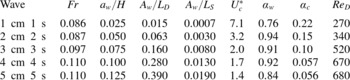
Five wave–current flow conditions were used (see table 4). All flow conditions used the same pump rate, so they had similar freestream current velocities. The mean water depth was
 $H=0.4~\text{m}$
in all cases, indicating that the canopy was in the shallow submergence regime (
 $H/h\approx 2.6$
), but it was far from being emergent (Nepf Reference Nepf2012). Progressive surface waves were generated using a vertical plunger-style wavemaker, which is situated at the upstream end of the flume. All waveforms were designed to have similar slope, so the wave amplitude,
 $a_{w}$
, in centimetres was tuned to match the wave period,
 $T$
, in seconds. The wave cases are referred to by their amplitude and period (i.e. ‘1 cm 1 s’, ‘2 cm 2 s’, etc.). Owing to amplitude dispersion and the complex geometry of the flume, the shapes of the waves had to be optimized empirically. This was done by assuming that all of the distortion of the wave was caused by amplitude dispersion according to the Korteweg–de Vries (KdV) equation. The KdV equation was integrated in reverse to determine the wave shape that needed to be created at the plunger to get a symmetric wave at the sampling location. Time-integrating the surface displacement gave the wavemaker displacement required to create the wave. This process had to be done iteratively, but proved to be an effective method for creating the desired waveforms. The waves were evaluated using a capacitance wave gage. Before each experiment, they were allowed to come to a steady state, which took a few minutes for the largest waves.
Velocity measurements were taken using a Nortek Vectrino acoustic velocimeter (ADV) and a particle image velocimetry (PIV) system composed of a New Wave Gemini laser and a LaVision imaging system. The primary purpose of the PIV measurements was to generate true volume-averaged statistics within the canopy. The ADV measurements were used to increase vertical and temporal resolution and to capture vertical velocities. All measurements were synchronized through the wavemaker control system. The servo controller (National Instruments PCI-7342) was programmed to treat the wavemaker motion and the measurement triggering as two-axis motion, allowing extremely precise synchronization. This was critical to computing accurate ensemble-averaged phase-dependent turbulence statistics.
The ADV was mounted to a 2D Cartesian robot to allow precise, automated profiling. ADV measurements were taken at 19 heights between 3 and 30 cm above the bottom with 1 cm resolution near the top of the canopy. The ADV was located at the midpoint between diagonally adjacent elements in the centre of the steel plate region. The ADV was operated at 100 Hz and 256 waves were sampled in each flow condition. The ADV data was cleaned with iterative statistical outlier detection with no filling of missing data.
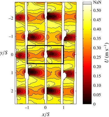
PIV measurements were taken in 7 horizontal planes at 2, 5, 8, 10, 12, 14, and 16 cm above the bottom. The laser sheet entered through the glass sidewall of the flume. The camera imaged through the flume’s glass bottom and the acrylic mounting sheet. The positions of the steel elements were adjusted to minimize shadows in the laser sheet. The camera was centred directly below one of the elements to minimize obstruction of the imaging plane. These adjustments allowed imaging of almost the entire in-canopy region (see figure 4), which was critical for computing volume-averaged statistics. A total of 128 waves were sampled, except in the 1 cm 1 s wave case, where 256 waves were sampled. Image pairs were captured at 10 Hz every third wave to allow time for data to transfer from memory to storage on the computer. The PIV images were processed with LaVision’s DaVis PIV software. The images were pre-processed with intensity normalization and masking of shadow regions. Multipass PIV with 50 % overlap was used to compute the vector fields. In post-processing, outliers were removed and replaced with interpolated values. The vector fields were smoothed with a filter that was chosen so that the sides were shorter than the laser sheet thickness.
Example PIV data for the streamwise velocity ensemble-averaged by wave phase,
 $U~(\text{m}~\text{s}^{-1})$
. The data was taken in the 5 cm 5 s wave condition at 14 cm above the bottom. The laser sheet enters from the positive
 $y$
direction. The vertical white streaks are regions that were masked during image pre-processing because they were in the shadows that the elements created in the laser sheet. The masked regions were filled with interpolated data, except in the immediate vicinity of the elements. The rectangle in the centre of the image indicates the ROI that was used for volume-averaging.

The data was ensemble-averaged by wave phase to get unsteady Reynolds-averaged statistics. This procedure represents a straightforward, rigorous wave–turbulence decomposition. For volume-averaging, an image processing algorithm was developed to identify a region of interest (ROI) around the centre element in the PIV data. The region was rectangular with an extent of
 $2S$
in the
 $x$
direction and
 $S$
in the
 $y$
direction. This represents a symmetric region that is spatially periodic throughout the canopy. Thus, averaging over the ROI is a reasonable approximation of the volume average, as defined in Finnigan (Reference Finnigan2000).
All flow statistics were computed using a combination of PIV and ADV measurements, then interpolated onto a 1 cm resolution grid to allow straightforward depth averaging. For
 $z\leqslant 16~\text{cm}$
,
 $\langle U\rangle$
and
 $\langle V\rangle$
were computed from direct volume averaging of the PIV data and for
 $z>16~\text{cm}$
they were computed from ADV measurements. Bootstrapping was used to compute confidence intervals for each
 $\langle U\rangle$
value from PIV within the canopy and the mean 95 % confidence interval was
 $\pm 1.6\times 10^{-4}~\text{m}~\text{s}^{-1}$
. Estimates of
 $\langle W\rangle$
were computed from the ADV measurements by assuming that
 $W$
was horizontally homogeneous. The horizontal Reynolds stresses and horizontal gradients of
 $U$
and
 $V$
from PIV were used to compute
 $\mathscr{P}_{w}$
. ADV measurements alone were used to compute
 $\overline{u^{\prime }w^{\prime }}$
, which was used as an estimate of
 $\langle \overline{u^{\prime }w^{\prime }}\rangle$
at each height. The shear layer turbulence dominates
 $\langle \overline{u^{\prime }w^{\prime }}\rangle$
and should not be influenced by inter-element variability. Although capacitance wave gauge measurements were available, the pressure gradient was computed using the momentum budget above the canopy where there is no drag. The time-averaged component of
 $\partial P/\partial x$
was two orders of magnitude smaller than the phase-dependent component. The relationship from linear wave theory,
 $[\partial P/\partial x]_{w}\propto \cosh (k_{w}z)$
, was fit to the wave-driven pressure gradient estimates and the time-averaged component was added back in to give the pressure gradient profile over the full water column at each wave phase.
3. Results and discussion
3.1. Basic results
Example PIV data is provided in figure 4 to demonstrate the shadow minimization and volume-averaging techniques. Basic laboratory results for the largest waves are presented in figure 5. Here
 ${\it\theta}$
is defined so that
 $\widehat{U}$
transitions from negative to positive at
 ${\it\theta}=0$
and
 $\langle U\rangle$
and
 $\langle W\rangle$
were approximately 90° out of phase as predicted by linear wave theory. The in-canopy PIV measurements of
 $\langle U\rangle$
were roughly 10 % smaller than
 $U$
measured by the ADV in all cases. This is because the ADV measurements were taken outside the wake, which is standard practice. Using the true volume average from PIV led to smaller, more uniform in-canopy
 $\langle U\rangle$
than in previous studies and more highly concentrated shear at the top of the canopy. The Reynolds stress lagged behind the shear and spread vertically as it was generated. There were also slight downward and upward movements of the Reynolds stress peak, which correspond with the negative and positive values of
 $\langle W\rangle$
.
Example results from the 5 cm 5 s flow condition: (a)
 $\langle U\rangle ~(\text{m}~\text{s}^{-1})$
; (b)
 $\langle W\rangle ~(\text{m}~\text{s}^{-1})$
; (c)
 $\partial \langle U\rangle /\partial z~(\text{s}^{-1})$
; (d)
 $-\langle \overline{u^{\prime }w^{\prime }}\rangle ~(\text{m}^{2}~\text{s}^{-2})$
. These results were computed and interpolated from a combination of PIV and ADV measurements as described in § 2.

3.2. Momentum budget scaling
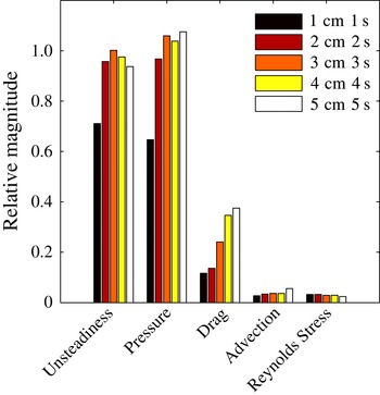
In order to quantify the relative magnitudes of the momentum budget terms, the r.m.s. in-canopy depth average of each term was non-dimensionalized by
 ${\it\omega}U_{w}$
(see figure 6). The results confirmed the hierarchy predicted by the proposed momentum budget scaling: unsteadiness
 ${\sim}$
pressure
 $\gg$
drag
 $\gg$
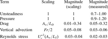
advection, Reynolds stress. The influence of wave size on the relative magnitudes of the momentum budget terms was also consistent with the proposed scaling. The scale for each term based on (1.33) is summarized in table 5. The values of the non-dimensional flow parameters for the five wavy flow conditions are listed in table 6.
Relative magnitudes of the momentum budget terms for the 5 wavy flow conditions. The magnitudes were computed by taking the RMS in-canopy depth-average of each term and non-dimensionalizing by
 ${\it\omega}U_{w}$
. The drag is based on the residual of the momentum budget.

Summary of the scale for each term based on (1.33).

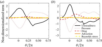
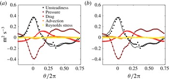
Example non-dimensionalized in-canopy depth-averaged momentum budgets (1.33) for (a) the 2 cm 2 s wave case and (b) the 5 cm 5 s wave case as a function of wave phase. Each term is non-dimensionalized by
 ${\it\omega}U_{w}$
. All terms were moved to the left-hand side of (1.33), so their sum should be zero. There is a clear balance between pressure and unsteadiness, modulated by drag.

Summary of the parameters for the five flow conditions. For reference,
 $L_{D}=26~\text{cm}$
and
 $L_{S}=5.4~\text{m}$
based on
 $C_{D}=1$
and
 $C_{S}=0.17$
.

Unsteadiness and pressure represent the dominant balance in the proposed scaling, so they are always
 $O(1)$
. This was confirmed by the experimental results. The drag was the next largest term. According to the scaling, its magnitude should have varied from 0.01 to 0.34. The experimental results generally agree. The smallest value was slightly larger (approximately 0.05), which can be attributed to the current inside the canopy. For the smallest waves,
 $U_{c}^{\ast }\approx 7$
, violating the assumption that
 $U_{c}^{\ast }\sim O(1)$
, which was used to justify the assertion that the in-canopy current can be neglected. The magnitude of the drag increased with wave size because of the increasing
 $A_{w}$
. Vertical advection and Reynolds stress were much smaller and had similar magnitudes according to both the scaling and the experiments. The vertical advection increased as wave size increased because of the increase in
 $\mathit{Fr}$
. The Reynolds stress remained almost constant as the wave size increased because the increase in
 $A_{w}$
was balanced by the decrease in
 ${U_{c}^{\ast }}^{2}$
.
Examples of phase-dependent in-canopy momentum budgets are provided in figure 7, demonstrating balances that are dominated by unsteadiness and pressure modulated by drag. Based on the proposed scaling, this type of balance is expected to be representative of many combined wave–current flows and was likely present in previous experimental studies, such as Lowe et al. (Reference Lowe, Koseff and Monismith2005, Reference Lowe, Shavit, Falter, Koseff and Monismith2008), Luhar et al. (Reference Luhar, Coutu, Infantes, Fox and Nepf2010) and Pujol et al. (Reference Pujol, Serra, Colomer and Casamitjana2013). However, this was not clear because the studies did not present phase-dependent momentum budgets or hierarchies of the terms.
3.3. Parameterization testing
3.3.1. Drag
The volume-averaged momentum budget was used to estimate
 $F_{D}(z,{\it\theta})$
in each flow condition. The quadratic drag parameterization was fit to the results of all of the experiments, which yielded
 $C_{D}=2.4$
. This value was a good fit for each individual experiment as well. The
 $R^{2}$
values for the parameterization and the momentum budget residuals were
 $R^{2}=0.71$
for
 $\widehat{F}_{D}({\it\theta})$
and
 $R^{2}=0.84$
for
 $F_{D}(z,{\it\theta})$
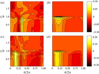
. The quadratic drag parameterization and the momentum budget estimates agree on the rough qualitative features of
 $F_{D}(z,{\it\theta})$
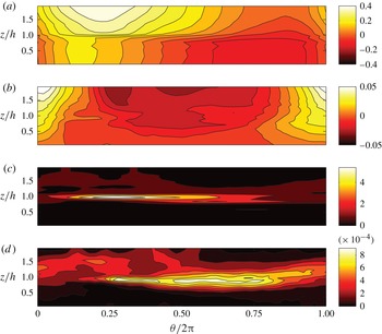
, namely the two pulses of high drag when the fluid velocity has its positive and negative peaks (see figure 8). However, the more detailed features of
 $F_{D}(z,{\it\theta})$
are significantly different in the two estimates. The momentum budget estimates suggest that the positive pulse in
 $F_{D}({\it\theta})$
at
 ${\it\theta}/2{\rm\pi}\approx 1/4$
has a sharp peak and that
 $F_{D}(z)$
at that phase is maximized below the top of the canopy, near
 $z/h=0.8$
. The parameterization suggests that the pulses in
 $F_{D}({\it\theta})$
are much smoother and that
 $F_{D}(z)$
is always maximized at the top of the canopy. Both of these inconsistencies were observed in all flow conditions and they can be attributed to the assumption of constant drag for the
 $C_{D}$
parameterization. Studies of finite-aspect-ratio flat plates oriented normal to unsteady flow have shown that
 $C_{D}$
depends on the aspect ratio of the plate, the end conditions and the vortex formation time (Ringuette Reference Ringuette2004; Ringuette, Milano & Gharib Reference Ringuette, Milano and Gharib2007).
Estimates of
 $F_{D}~(\text{m}^{2}~\text{s}^{-1})$
for the (a,b) 2 cm 2 s wave case and (c,d) the 5 cm 5 s wave case estimated from (a,c) the momentum budget (1.1) and (b,d) the quadratic drag parameterization (1.10) with
 $C_{D}=2.4$
. The momentum equation
 $F_{D}$
shows a more concentrated positive peak as a function of
 ${\it\theta}$
. At the top of the canopy, the momentum equation suggests that
 $F_{D}$
drops off sharply, whereas the parameterization suggests that it has a sharp increase.

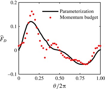
Comparison between the momentum budget and quadratic drag parameterization estimates of
 $\widehat{F}_{D}$
as a function of wave phase. The value of
 $C_{D}=2.4$
was chosen by fitting the quadratic drag parameterization to the local
 $F_{D}$
values for all flow cases.

The elements in the present study have a large aspect ratio (
 $h/D\approx 24$
), a free end at the top of the canopy and a fixed end at the bottom. The portion of the element that is far from the free end should have a 2D wake, resulting in a large
 $C_{D}$
. However, near the free end, the flow is 3D and
 $C_{D}$
should be much smaller. For reference, a single flat plate normal to steady, high-
 $\mathit{Re}$
flow has
 $C_{D}=2.3$
when
 $h/D=\infty$
and
 $C_{D}=1.5$
when the plate has one free end and
 $h/D=1$
(Ringuette Reference Ringuette2004; Narasimhamurthy & Andersson Reference Narasimhamurthy and Andersson2009). This reduction in
 $C_{D}$
at the top of the canopy explains why the momentum budget estimate of
 $F_{D}$
demonstrates a maximum below the top of the canopy, whereas the
 $C_{D}$
parameterization incorrectly predicts a maximum at
 $z=h$
.
The unsteadiness of the flow adds further error into the constant
 $C_{D}$
assumption (1.10). When the flow accelerates and decelerates, wake development lags behind the changes in
 $\langle U\rangle$
, violating the quasi-steady assumption. The sharper peak in the momentum budget estimates of
 $F_{D}$
as compared with the parameterization estimates (see figures 8 and 9), is consistent with the observations of Ringuette (Reference Ringuette2004). When the flow is accelerating, the undeveloped wakes result in anomalously high
 $C_{D}$
. As
 $\langle U\rangle$
reaches its maximum value, the wakes are allowed to develop and
 $C_{D}$
relaxes to its quasi-steady value. The resulting correlation between
 $C_{D}$
and
 $\langle U\rangle$
causes a sharp peak in drag. Unsteady wake effects for a single element are typically quantified by using the eddy turnover time to non-dimensionalize the time that the wake has had to develop, resulting in quantities such as the Keulegan–Carpenter number and the vortex formation time (Dalrymple & Dean Reference Dalrymple and Dean1991; Ringuette Reference Ringuette2004). This deserves further exploration in canopies, where multiple length scales are at play.
While the above explanations are based on previous studies of drag on a single element, there are many more complexities that could influence
 $C_{D}$
in wave-driven canopy flow. Horizontal variability of
 $U$
, vertical shear, wave-induced
 $W$
and interaction between shear and wake turbulence may all have an influence on the apparent
 $C_{D}(z,{\it\theta})$
. While it is beyond the scope of this paper, the
 $C_{D}$
parameterization needs to be improved for applications where accurate high-resolution local
 $F_{D}$
values are critical, such as biomechanical failure analysis. Accounting for the end condition, aspect ratio and unsteadiness effects may be appropriate initial improvements.
The constant
 $C_{D}$
approximation is more appropriate when the application only requires an accurate estimate of
 $\langle U\rangle$
, especially at low resolution. This is because
 $\langle U\rangle$
depends on the cumulative effect of
 $F_{D}$
, rather than the instantaneous value. Because the influence of unsteadiness on
 $C_{D}$
primarily causes the peaks in
 $F_{D}({\it\theta})$
to sharpen, the constant
 $C_{D}$
approximation essentially acts as a low-pass filter on
 $F_{D}({\it\theta})$
.
The assumption of uniform in-canopy
 $\langle U\rangle$
for estimating drag in a 2-box model (1.11) was evaluated using the laboratory measurements. The estimate is extremely accurate, with
 $R^{2}=0.997$
. The accuracy can be attributed to the dominance of the wave-induced velocity inside the canopy. The time-averaged velocity increases rapidly as it nears the top of the canopy. However, this vertical variability is small compared with the large swings in the wave-induced velocity, which are uniform with depth. Thus, vertical variability of
 $\langle U\rangle$
is not a significant source of error in the drag parameterization. In reality, the error would be reduced even further by the free end condition at the tops of the elements because reduction in the apparent drag coefficient would counteract the anomalous velocities near the top of the canopy.
3.3.2. Reynolds stress
The Reynolds stress measured by the Vectrino at
 $z=16~\text{cm}$
was used as an estimate of
 $-\langle \overline{u^{\prime }w^{\prime }}\rangle _{h}$
in order to assess the Reynolds stress parameterizations in the context of a 2-box model. This test case was chosen because the top of the canopy is the most important and most difficult location to estimate the Reynolds stress.
The
 $C_{f}$
parameterization (1.18) was compared with experimental data (see figure 10). The value of
 $C_{f}$
was chosen to match the time average of the parameterization to the time-averaged Reynolds stress in the 5 cm 5 s case. This strategy was selected because it represents one method that could be used in situations where phase-dependent data is unavailable. The
 $C_{f}$
parameterization fails to capture the variability in
 $-\langle \overline{u^{\prime }w^{\prime }}\rangle _{h}$
. The variation in
 $U_{\infty }$
is disproportionately large compared with the variation in
 $-\langle \overline{u^{\prime }w^{\prime }}\rangle _{h}$
, and the two statistics are poorly correlated. This is because
 $-\langle \overline{u^{\prime }w^{\prime }}\rangle _{h}$
is created by the velocity deficit. Here
 $U_{\infty }$
is not a good predictor of the velocity deficit because the waves induce large variations in velocity that are fairly uniform throughout the water column. In unidirectional cases, the
 $C_{f}$
parameterization works well because
 $\widehat{U}$
is small compared with
 $U_{\infty }$
(Grimmond & Oke Reference Grimmond and Oke1999). However, the parameterization is clearly inappropriate for flows with significant wave forcing.
Reynolds stress measurements compared with the
 $C_{f}$
parameterization for
 $C_{f}=0.025$
. In order to take advantage of the higher sampling rate of the ADV, only ADV data was used for this figure. This is appropriate because
 $U_{\infty }$
and
 $-\langle \overline{u^{\prime }w^{\prime }}\rangle _{h}$
do not require in-canopy volume averaging. The data parameterization passes near the centre of the data for each flow condition, but does not capture the variability with phase.

The 2-box Smagorinsky model (1.19) demonstrates much better performance because it uses a direct estimate of the shear (see figure 11). In the context of a 2-box model, the shear is estimated using the velocity deficit,
 $U_{\infty }-\widehat{U}$
. The value of
 $C_{S}$
was chosen to match the time average of the parameterization to the time-averaged Reynolds stress in the 5 cm 5 s case, giving
 $C_{S}=0.14$
. This is well within the typical
 $C_{S}$
range of 0.1–0.2 (Vreman et al.
Reference Vreman, Geurts and Kuerten1997). The error in this parameterization is analogous to the error attributed to unsteadiness in the drag parameterization. There is a small phase lag between
 $-\langle \overline{u^{\prime }w^{\prime }}\rangle _{h}$
and
 $U_{\infty }-\widehat{U}$
, which is reasonable because the anisotropy does not instantaneously adjust to changes in shear. In addition, the phase lag is smaller when the shear increases and larger when the shear decreases. This is because the development of anisotropy and the return to isotropy occur by two different mechanisms: rapid pressure–strain correlation and slow pressure–strain correlation (Pope Reference Pope2000). The former acts on a time scale associated with the shear and the latter acts on a time scale associated with the turbulence. Similarly, the peak in
 $-\langle \overline{u^{\prime }w^{\prime }}\rangle _{h}$
near
 ${\it\theta}/2{\rm\pi}=0.3$
results because the production of turbulence lags behind the sudden increase in shear, so the rapid pressure–strain correlation is briefly dominant over slow pressure–strain correlation.
Comparison of the
 $C_{f}$
and Smagorinsky parameterizations with
 $-\langle \overline{u^{\prime }w^{\prime }}\rangle _{h}$
measurements from the 5 cm 5 s flow case. Here
 $C_{f}=0.025$
and
 $C_{S}=0.14$
were used. The parameterization values were computed using the combined ADV and PIV data, whereas
 $-\langle \overline{u^{\prime }w^{\prime }}\rangle _{h}$
was computed from ADV measurements alone.

The errors due to the Reynolds stress adjustment time are exacerbated in the higher-frequency waves because the wave time scales are closer to the turbulence time scale, but the Smagorinsky model always performs much better than the quadratic friction parameterization. The turbulence time scale effects are precisely what 1- and 2-equation models attempt to capture. However, based on the result that Reynolds stress accounts for less than 5 % of the momentum budget, modelling the turbulence time scale is unnecessary. Furthermore, both the accuracy of the Smagorinsky model and the significance of the Reynolds stress are expected to increase with increasing
 $A_{w}/L_{S}$
, so the parameterization is more accurate when accuracy is more important.
3.3.3. Vertical advection
The proposed parameterization for vertical advection was evaluated for implementation in both high- and low-resolution models. These can be seen as upper and lower bounds on the accuracy of the parameterization.
For
 $[\langle U\rangle \langle W\rangle ]_{h}$
,
 $\langle W\rangle$
was estimated using two different methods in order to evaluate the assumption that pressure balances unsteadiness. In order to estimate
 $\langle W\rangle$
directly from unsteadiness, the phase speed of the waves estimated from linear wave theory was used to substitute unsteadiness into (1.13). The second method is the proposed parameterization, which uses the depth-integrated pressure as a proxy for the depth-integrated unsteadiness (see (1.16)). Qualitatively, there is little difference in the accuracy of the two estimates (see figure 12). The phase-dependent estimates contain two interesting features relative to the measured values. First, the measurements demonstrate
 ${\sim}$
1 s long fluctuations that are not mimicked accurately by the estimates. These may be caused by ejection of fluid out of the canopy or entrainment of fluid in the element wakes. Second, there is a phase-lag when the vertical velocity is increasing most rapidly. Based on linear wave theory, this is coincident with the maximum surface displacement. This suggests that the phase lag may be caused by nonlinearity of the waves, which would cause the phase speed during the maximum surface displacement to be larger than the phase speed based on linear wave theory.
Estimated and measured advective flux as a function of wave phase for the 5 cm 5 s flow condition. Estimates based on integrating the pressure gradient (1.15) are provided, as well as estimates based on directly integrating the unsteadiness. The difference is that the pressure estimate assumes that pressure balances unsteadiness.

Because
 $\langle W\rangle$
alone may be important in some applications, estimates of
 $\langle W\rangle$
were compared with measurements, giving
 $R^{2}=0.93$
. When the vertical advection parameterization was tested directly, the
 $R^{2}$
value was 0.96 (see figure 13). The improvement suggests that the
 $\langle W\rangle$
estimate is more accurate when the flux is stronger.
Estimates of advective flux compared with measurements from all wave cases at all heights. Estimates are based on the
 $\langle W\rangle$
parameterization (1.15) and measured
 $\langle U\rangle$
values.

The 2-box model was used to evaluate the parameterization in the context of a low-resolution model (see figure 14). This gives a lower bound on the accuracy of finite-volume approximations for the vertical advection. The estimated versus measured momentum flux into the canopy had an
 $R^{2}$
value of 0.77. One might assume that the spatial discretization causes the increase in error. However, further analysis indicated that the true cause was that the
 $\langle W\rangle$
parameterization was less accurate at the top of the canopy than at other locations.
Estimated advective flux at the top of the canopy compared with measurements for all wave cases. Estimates are based on the parameterization of
 $\langle W\rangle$
and spatial interpolation of
 $\langle U\rangle$
presented in (1.16).

3.3.4. Wake production
Direct measurements of
 $\mathscr{P}_{w}$
were used to assess the accuracy of the
 $C_{D}$
parameterization. The cubic proportionality appropriately captures the trend in the relationship between
 $\mathscr{P}_{w}$
and
 $\langle U\rangle$
(see figure 15). However, there is significant spread in the data. Many of the measured
 $\mathscr{P}_{w}$
values are less than 50 % of the predicted value. In figure 16, estimated values and measured values are plotted as a function of time. There is a lag between
 $\mathscr{P}_{w}$
and
 $|\langle U\rangle |^{3}$
, which is attributed to the finite time required for the wakes to develop. The eddy turnover time of the wake scale eddies,
 $D/U_{w}$
, is a logical time scale for estimating the lag. Based on observations from the five flow conditions, the lag is approximately
 $3D/U_{w}$
. The
 $C_{D}$
parameterization was greatly improved by incorporating this small lag time (see figure 17). The value of
 ${\it\beta}_{p}$
was chosen by fitting the
 $\mathscr{P}_{w}$
parameterization to the data while using the
 $C_{D}=2.4$
value that was computed for the quadratic drag parameterization.
The
 $C_{D}$
parameterization for
 $\mathscr{P}_{w}$
compared with measurements from the five flow conditions. Here
 $C_{D}=2.4$
was chosen to match the
 $F_{D}$
parameterization and
 ${\it\beta}_{p}=0.8$
was chosen to match the
 $\mathscr{P}_{w}$
data.

Lagged and unlagged versions of the in-canopy depth-averaged
 $C_{D}$
parameterization for
 $\mathscr{P}_{w}$
compared with data for the 5 cm 5 s wave case. Here
 $C_{D}=2.4$
and
 ${\it\beta}_{p}=0.8$
. The phase lag is
 ${\it\theta}/2{\rm\pi}=0.02$
, which is equivalent to 0.1 s.

Lagged
 $C_{D}$
parameterization for
 $\mathscr{P}_{w}$
compared with measurements from the five flow conditions. Here
 $C_{D}=2.4$
,
 ${\it\beta}_{p}=0.8$
and the parameterization is lagged
 ${\it\theta}/2{\rm\pi}=0.02$
(0.1 s).

3.3.5. Shear production
The shear production parameterization was evaluated by comparing it with the average measured
 $\mathscr{P}_{s}$
between
 $z=(3/4)h$
and
 $z=(5/4)h$
(see figure 18). This region was chosen by assuming that
 $\mathscr{P}_{s}$
happens almost entirely within a quarter canopy height of the top of the canopy. The
 $C_{S}$
value was chosen to be 0.14 based on the Reynolds stress parameterization. The
 ${\it\delta}_{S}$
value was chosen to give the same r.m.s. value as the measurements. This yielded
 ${\it\delta}_{S}=0.65h$
, which is a reasonable length scale for the mixing layer shear. Once the magnitude of the parameterization was scaled appropriately, the shape showed good agreement with the shape of the measured values. There is a phase lag that varies with phase, similar to the lag seen in the Reynolds stress estimate. It is logical that
 $\mathscr{P}_{s}$
would take a finite time to react to changes in shear. As with the Reynolds stress, the lag during increasing shear is smaller than the lag during decreasing shear, corresponding to rapid and slow pressure–strain correlation, respectively. While the utility of the
 $\mathscr{P}_{S}$
parameterization is diminished by the need for empirical fitting, these results demonstrate the general concept that
 $\mathscr{P}_{S}\sim |U_{\infty }-\widehat{U}|^{3}/h$
.
Mixing layer
 $\mathscr{P}_{s}$
estimates from the Smagorinsky parameterization for the 2-box model compared with laboratory measurements from the 5 cm 5 s flow condition. The mixing layer is assumed to be the region within
 $0.25h$
of the top of the canopy. The value of
 $C_{S}=0.14$
was chosen based on the results for the Reynolds stress and the value of
 ${\it\delta}_{S}=0.65h$
was chosen by matching the r.m.s. of the parameterization to the r.m.s. of the measurements.

3.4.
$N$
-box model

Four different implementations of the N-box model were used to explore the trade-offs between simplicity, resolution, and accuracy. The implementations have only two distinguishing features:
-
(a) the number and location of box faces and
-
(b) the choice of explicit or implicit filtering for the Reynolds stress parameterization.
Based on these distinctions, the models were given the following names: 2-box implicit (2BI), high-resolution implicit (HRI), high-resolution explicit (HRE) and non-uniform-resolution implicit (NRI). The order of this list represents sequential adjustments to the model in order to accurately resolve the in-canopy velocity while minimizing complexity. The accuracy of each implementation was evaluated through comparison with laboratory measurements from the largest wave condition. Table 7 summarizes the four models and figure 19 provides a representation of how each model performs at a single snapshot in phase.
Example output from each of the four models at a single snapshot in phase: (a) 2BI; (b) HRI; (c) HRE; and (d) NRI. The vertical lines are used to denote the extent of each box and the dots denote the nodes.

Summary of the four implementations of the N-box model that were tested. The
 $R^{2}$
values are based on comparison with all of the
 $\langle U\rangle$
measurements from the five flow conditions.

2BI consists of two boxes with faces at the bottom boundary, the top of the canopy, and the mean water surface. 2BI is similar to the 2-box model from Lowe et al. (Reference Lowe, Koseff and Monismith2005). However, 2BI (a) uses the Smagorinsky model rather than the
 $C_{f}$
parameterization for Reynolds stress, (b) includes vertical advection based on linear wave theory and (c) takes a pressure gradient as an input instead of the above-canopy velocity. 2BI accurately represents the variability of the above- and in-canopy velocities. The obvious shortcoming of the model is that it does not resolve the transition region from low velocity inside the canopy to high velocity above.
HRI was designed to resolve the velocity transition by (naively, in retrospect) increasing the resolution to
 ${\rm\Delta}z=h/8$
, giving 16 boxes from
 $z=0$
to
 $z=2h$
. The velocity estimates at the top of the canopy were improved. However, with increasing height above the canopy, the model increasingly overestimated the velocity. This was caused by underestimates of the Reynolds stress because the filter length was assumed to be equal to the length scale of the spatial discretization. An implicit filter is inappropriate in HRI because of the large eddies that dominate above the canopy. The N-box model does not simulate these eddies and they are not accounted for in the Reynolds stress parameterization.
In HRE, an explicit filter was implemented in order to reduce the errors in HRI caused by the implicit filter. The Smagorinsky model with explicit filtering is defined as follows (Vreman et al. Reference Vreman, Geurts and Kuerten1997):
 $$\begin{eqnarray}{{\it\tau}_{xz}}_{i+(1/2)}=\left(\frac{C_{S}{\it\Delta}}{{\rm\Delta}z}\right)^{2}\left|U_{i+1}-U_{i}\right|(U_{i+1}-U_{i}).\end{eqnarray}$$
For HRE,
 ${\it\Delta}$
was specified as a piecewise function that represents the largest possible scale of eddies:
 $$\begin{eqnarray}{\it\Delta}=\left\{\begin{array}{@{}ll@{}}{\it\delta}_{e}\quad & \text{if }z\leqslant h-{\it\delta}_{e}\\ z-h+{\it\delta}_{e}\quad & \text{if }h-{\it\delta}_{e}<z\leqslant \displaystyle \frac{H+h-{\it\delta}_{e}}{2}\\ H-z\quad & \text{if }\displaystyle \frac{H+h-{\it\delta}_{e}}{2}<z\end{array}\right.\end{eqnarray}$$
where the penetration depth,
 ${\it\delta}_{e}\approx (1/6)L_{D}$
, represents the distance to which vortices can penetrate into the canopy (Ghisalberti Reference Ghisalberti2009). Equation (3.2) shows that
 ${\it\delta}_{e}$
is mainly important because it determines the maximum eddy size above the canopy where the velocity gradients are strongest. The chosen filter length profile implicitly assumes that the turbulence is fully developed, which may seem like a poor assumption in a flow that has significant wave forcing that could modulate the eddy scales. In reality, even for strong wave forcing, the shear is current-dominated, which means that the dominant eddies are fully developed. Thus, the explicit filter in (3.2) significantly reduces the error in the above-canopy velocities. It was only validated for one canopy, so it is not necessarily generalizable and results near the free surface are sensitive to the explicit filter, so it will need to be validated using a specialized technique that can capture measurements near the free surface in waves. However, the results show that a simple, a priori choice for the filter can produce accurate results and that turbulence length scale modulation by the waves can be ignored when the shear is current-dominated.
For some applications, it is important to have high resolution inside the canopy, but not above. This may be the case when estimating nutrient uptake or sediment transport, especially when the canopy density varies with depth. NRI addresses this situation through non-uniform resolution. NRI has high resolution inside the canopy (
 ${\rm\Delta}z=h/8$
), and a single cell above the canopy
 $({\rm\Delta}z=h)$
. Inside the canopy, eddies are restricted in size by the element spacing, so the implicit filter remains accurate at high resolution. Above the canopy, the implicit filter can be used because of the low resolution. NRI provides accurate estimates of the in-canopy velocity profile, as well as the average velocity between
 $z=h$
and
 $z=2h$
. NRI is closely related to the 3-box model of Weitzman (Reference Weitzman2013) and Weitzman et al. (Reference Weitzman, Zeller, Thomas and Koseff2015), which employs two in-canopy boxes to account for polycultural vegetation with a sparse upper canopy and a dense understory. NRI demonstrates how the N-box model could be used to generalize the 3-box approach to incorporate higher-resolution vegetation density profiles.
The above observations indicate the trade-offs that should be considered when implementing an N-box model. 2BI, HRE and NRI represent three strategies that are appropriate in different situations. The accuracy of HRE mostly depends on the choice of explicit filter. The accuracies of 2BI and NRI are explored further below.
2BI and NRI demonstrated similar accuracy as a function of phase for locations far above the canopy and deep inside the canopy. The main advantage of NRI is the point at the top of the canopy that captures the transition between the above-canopy and in-canopy velocity (see figure 20). The phase-dependent momentum budgets for 2BI’s in-canopy box and NRI’s
 $z=h/2$
box were evaluated against laboratory results (see figure 21). The two models’ momentum budgets show almost identical behaviour and both models qualitatively capture the behaviour seen in the laboratory results. Figure 21 demonstrates the core reason that a simple N-box model works: vertical advection and Reynolds stress are small compared with drag. Since the pressure gradient is an input, the drag is the most important parameterization for estimating unsteadiness. Based on visual inspection of figure 21, most of the error seems to come from measurement uncertainty and the drag parameterization. The error due to the Reynolds stress and vertical advection parameterizations is small.
The
 $N$
-box model results for the streamwise velocity as a function of phase compared with laboratory results from the 5 cm 5 s flow condition: (a) 2BI and (b) NRI. The lines represent model results and the dots represent laboratory results.

Modelled momentum budget terms as a function of phase compared with laboratory results from the 5 cm 5 s flow condition: (a) 2BI’s in-canopy box and (b) NRI’s box between
 $3h/8$
and
 $h/2$
. The lines represent model results and the dots represent laboratory data.

Results from 2BI, HRI, HRE and NRI were compared against all of the corresponding measurements for the five flow conditions and
 $R^{2}$
values were computed. 2BI had
 $R^{2}=0.98$
, HRI had
 $R^{2}=0.68$
, HRE had
 $R^{2}=0.98$
and NRI had
 $R^{2}=0.98$
. The comparison between HRE estimates and measured values is shown in figure 22. While the 2BI, HRE and NRI implementations of the N-box model have been shown to be effective in a limited range of conditions, the broader implication is that when a simple, standard turbulence model is used, it is not the dominant source of error. HRE is accurate without accounting for features such as unsteady turbulence time scales or non-local generation of wake scale kinetic energy because these features are irrelevant to the large-scale flow structure. In general, complexity and computational cost should be carefully weighed against accuracy when specialized turbulence models are developed for canopy flows.
The
 $\langle U\rangle$
values modelled by HRE compared with laboratory measurements for all five flow conditions.

4. Conclusions
Laboratory experiments were used to evaluate scaling, parameterizations and a simple model for combined wave–current canopy flow. The scaling indicates that pressure-driven unsteadiness modulated by drag accounts for the vast majority of the momentum budget in a large range of parameter space. Parameterizations for drag, Reynolds stress, vertical advection, wake production and shear production were evaluated. The results were used to develop a simple N-box model that predicts streamwise velocity profiles and is expected to be effective in a wide range of wave-driven canopy flows with a background current.
4.1. Scaling
Scaling was used to show that the following hierarchy of terms is applicable to a large region of parameter space that is relevant to natural aquatic canopies under shallow submergence exposed to wind waves and swell waves:
 $$\begin{eqnarray}\displaystyle \text{pressure }\sim \text{unsteadiness }\gg \text{drag }\gg \text{advection }\sim \text{Reynolds stress}. & & \displaystyle \nonumber\end{eqnarray}$$
The notion that Reynolds stress is negligible compared with drag has significant implications for modelling of wave-driven canopy flows. Namely, modelling of the shear scale turbulence is not expected to be the dominant source of error. Because shear-scale turbulence modelling accounts for most of the complexity in canopy flow models, the adjusted scaling implies that relatively simple models can be used to predict phase-dependent behaviour in combined wave–current canopy flows.
4.2. Parameterizations
A variety of parameterizations that are commonly used in canopy flows were assessed based on ADV profiles and horizontal PIV measurements. The parameterizations had not previously been tested independently in a canopy exposed to waves with a background current. Drag force, Reynolds stress and vertical advection parameterizations were tested for use in the momentum budget. Wake production and shear production parameterizations were also tested so TKE information could be extrapolated from volume-averaged streamwise velocity information.
The quadratic drag parameterization was found to be appropriate for estimating the rough qualitative behaviour of the drag and for use in predicting
 $\langle U\rangle$
. However, high-resolution estimates of
 $F_{D}$
contained errors caused by flow complexities such as unsteadiness and 3D effects. The vertical variability of the streamwise velocity was assessed in terms of its effect on the
 $F_{D}$
parameterization in a 2-box model. The error was found to be negligible because the wave velocity was fairly uniform with depth and was dominant over the current velocity.
Direct measurements of the Reynolds stress at the top of the canopy were compared with Reynolds stress parameterizations for a 2-box model. The quadratic friction model was unable to capture the true phase-dependence of the Reynolds stress. A parameterization based on the Smagorinsky model proved to be far more accurate.
Vertical advection was estimated by using shallow water wave theory to compute vertical velocity. In the context of the 2-box model it captured 77 % of the variability in vertical advection at the top of the canopy. Away from the top of the canopy it was much more accurate.
While the vertical advection and Reynolds stress parameterizations were the least accurate, the non-dimensional magnitudes of these terms were typically less than 5 %. Therefore the errors are small in the context of the full momentum budget.
The
 $\mathscr{P}_{w}$
parameterization was compared with direct measurements from PIV. The parameterization was fairly accurate, but demonstrated a small phase lag associated with wake development.
Here
 $\mathscr{P}_{s}$
was estimated using the Smagorinsky model for the 2-box model. The parameterization had to be fit to the measurements, but it was able to reproduce the general behaviour of the average
 $\mathscr{P}_{s}$
within the mixing layer.
4.3.
$N$
-box model

The scaling and parameterizations developed in the present study suggest that a relatively simple model is appropriate in wave-driven canopy flows. In order to leverage this finding, a simple N-box model was developed. The model is an extension and improvement over the 2- and 3-box models presented by Lowe et al. (Reference Lowe, Koseff and Monismith2005) and Weitzman et al. (Reference Weitzman, Zeller, Thomas and Koseff2015). The N-box model allows accurate prediction of the volume-averaged streamwise velocity profile based on a pressure gradient and a canopy density profile. The model is quick to implement, computationally efficient, and easy to interpret. Because of these qualities, the N-box model is a practical tool for a variety of applications; it could be used to interpret sparse field measurements, or to account for aquatic canopies in larger-scale numerical models.
Acknowledgements
We acknowledge W. Sabala, T. Mandel, A. Craig and I. Rozensweig for valuable discussion and for assistance with preparing the experiments. We also thank the associate editor, J. Riley, and three anonymous reviewers for their insightful and constructive comments. R. Zeller and J. Weitzman were supported by the Stanford Woods Institute for the Environment and F. Zarama was supported by a National Science Foundation Graduate Research Fellowship.