1. Introduction
When a perturbed interface separating two fluids of different densities is continuously accelerated from the light fluid towards the heavy one, Rayleigh–Taylor instability (RTI) occurs (Rayleigh Reference Rayleigh1883; Taylor Reference Taylor1950). This instability is driven by baroclinic vorticity arising from the misalignment of the pressure gradient and the local density gradient. Initially, perturbation growth enters a linear stage with an exponential growth rate. Then, in the nonlinear stage, large-scale finger structures of bubbles (light fluids penetrating into heavy fluids) and spikes (heavy fluids intruding into light fluids) emerge. The finger growth in this stage first follows an approximately constant rate, known as the quasi-steady stage, before potentially undergoing re-acceleration (Ramaprabhu et al. Reference Ramaprabhu, Dimonte, Young, Calder and Fryxell2006). Over time, these finger structures evolve across a wide range of scales, eventually transitioning to turbulence.
The RTI can be induced by various factors, most commonly by gravity. A typical occurrence in gravitational fields is the destabilisation of the interface when a heavy fluid is placed above a light fluid. Since the pioneering work of Rayleigh (Reference Rayleigh1883) and the modern development by Taylor (Reference Taylor1950), RTI under constant acceleration has been extensively investigated. Theoretically, several nonlinear models extended from the Layzer potential-flow framework (Layzer Reference Layzer1955) have been established to characterise the finger evolution during the quasi-steady stage (Hecht, Alon & Shvarts Reference Hecht, Alon and Shvarts1994; Alon et al. Reference Alon, Hecht, Ofer and Shvarts1995; Mikaelian Reference Mikaelian1998; Zhang Reference Zhang1998; Goncharov Reference Goncharov2002; Abarzhi Reference Abarzhi2003; Sohn Reference Sohn2003; Zhang & Guo Reference Zhang and Guo2016; Guo & Zhang Reference Guo and Zhang2020; Liu et al. Reference Liu, Wu-Wang, Zhang and Xiao2023a ,Reference Liu, Zhang and Xiao b ). Numerical studies have validated the asymptotic finger behaviour predicted by these nonlinear models (Ramaprabhu & Dimonte Reference Ramaprabhu and Dimonte2005; Zhou, Zhang & Tian Reference Zhou, Zhang and Tian2018), and a re-acceleration of the finger growth beyond the quasi-steady stage was observed (Ramaprabhu et al. Reference Ramaprabhu, Dimonte, Young, Calder and Fryxell2006; Wei & Livescu Reference Wei and Livescu2012; Bian et al. Reference Bian, Aluie, Zhao, Zhang and Livescu2020; Fu et al. Reference Fu, Zhao, Wang, Liu, Wan and Lu2023). The self-similar evolution of fingers in the turbulent mixing stage has been numerically investigated, with particular attention to the dependence of late-time mixing on initial conditions (Dimonte et al. Reference Dimonte2004; Ramaprabhu, Dimonte & Andrews Reference Ramaprabhu, Dimonte and Andrews2005; Cabot & Cook Reference Cabot and Cook2006; Youngs Reference Youngs2013). Experimentally, RTI has been explored in water and gas channels (Snider & Andrews Reference Snider and Andrews1994; Banerjee & Andrews Reference Banerjee and Andrews2006; Andrews & Dalziel Reference Andrews and Dalziel2010; Banerjee, Kraft & Andrews Reference Banerjee, Kraft and Andrews2010; Akula et al. Reference Akula, Suchandra, Mikhaeil and Ranjan2017) and in stationary tanks with a sliding plate separating two fluids (Linden, Redondo & Youngs Reference Linden, Redondo and Youngs1994; Jacobs & Dalziel Reference Jacobs and Dalziel2005; Lawrie & Dalziel Reference Lawrie and Dalziel2011). In these experiments, an initially random perturbation was typically introduced to investigate the development of large- and small-scale structures in the turbulent mixing stage. In addition, the magnetic levitation technique (Pacitto et al. Reference Pacitto, Flament, Bacri and Widom2000; Huang et al. Reference Huang, De Luca, Atherton, Bird, Rosenblatt and Carles2007; White et al. Reference White, Oakley, Anderson and Bonazza2010) and the soap-film technique (Liang et al. Reference Liang, Alkindi, Alzeyoudi, Liu, Ali and Masmoudi2024) have been employed to maintain a heavy fluid on top of a light one. These techniques allow for the creation of single-mode perturbations, enabling detailed examination of instability development across both linear and nonlinear regimes.
The RTI driven by time-dependent acceleration has been experimentally studied using gas guns (Kucherenko et al. Reference Kucherenko, Balabin, Cherret and Haas1997, Reference Kucherenko, Balabin, Ardashova, Kozelkov, Dulov and Romanov2003), rocket rigs (Read Reference Read1984; Youngs Reference Youngs1989) or linear electric motors (Dimonte et al. Reference Dimonte1996; Dimonte & Schneider Reference Dimonte and Schneider2000), with acceleration varying from tens to hundreds of times the gravitational acceleration. Random multi-mode perturbations were produced in these experiments to explore the RTI-induced turbulence. In contrast, single-mode perturbations were formed in drop tower experiments with low acceleration variations (0.33–1.35 times gravitational acceleration), and a detailed analysis of finger growth in the linear and nonlinear stages was conducted (Waddell, Niederhaus & Jacobs Reference Waddell, Niederhaus and Jacobs2001; Wilkinson & Jacobs Reference Wilkinson and Jacobs2007). Analytical models applicable to finger amplitudes and mixing layer widths across linear, nonlinear and turbulent regimes were developed by Mikaelian (Reference Mikaelian2014), who extended the potential-flow model of Layzer (Reference Layzer1955) to flows governed by time-dependent acceleration. Additionally, Ramaprabhu et al. (Reference Ramaprabhu, Karkhanis, Banerjee, Varshochi, Khan and Lawrie2016) derived two models for variable acceleration scenarios, with one based on the Layzer potential-flow framework for two-dimensional (2-D) bubbles, and the other employing a drag–buoyancy approach for both bubbles and spikes in two and three dimensions. The predictions from both models of Ramaprabhu et al. (Reference Ramaprabhu, Karkhanis, Banerjee, Varshochi, Khan and Lawrie2016) agreed well with the numerical counterparts under various time-dependent acceleration histories.
Differing from the RTI driven solely by constant or variable acceleration, rarefaction-driven RTI not only features variable acceleration but also incorporates time-dependent density (Gao et al. Reference Gao, Guo, Zhai and Luo2024), since the pressure in rarefaction regions decreases from the rarefaction head to the tail. In recent decades, rarefaction-driven RTI has received increasing attention due to its critical relevance in inertial confinement fusion (ICF) and air-breathing engines (Aglitskiy et al. Reference Aglitskiy2010; Zhou Reference Zhou2017a ,Reference Zhou b ; Urzay Reference Urzay2018; Zhou et al. Reference Zhou, Clark, Clark, Glendinning, Skinner, Huntington, Hurricane, Dimits and Remington2019, Reference Zhou2021, Reference Zhou, Sadler and Hurricane2025). In ICF, the laser-driven shock strikes the ablator/fuel interface, forming rarefaction waves that propagate back toward the ablation front. The interaction between these rarefaction waves and the ablation front leads to RTI-induced perturbation growth, enhancing mixing between the outer ablators and inner fuels, thereby reducing the fusion yield (Goncharov et al. Reference Goncharov, Skupsky, Boehly, Knauer, McKenty, Smalyuk, Town, Gotchev, Betti and Meyerhofer2000; Qiao & Lan Reference Qiao and Lan2021). In air-breathing engines, the rarefaction waves generated due to geometric corners or fuel injection create vorticity at the oxidiser/fuel interface, leading to mixing enhancement and thereby improving the propulsion efficiency (Li, Kailasanath & Book Reference Li, Kailasanath and Book1991; Li & Book Reference Li and Book1991). As a result, it is of significance to explore the mechanism of rarefaction-driven RTI.
The pioneering experimental studies on the rarefaction-driven RTI of liquid interfaces were performed by Lewis (Reference Lewis1950) in a rectangular tube connected to a large air reservoir. Their experimental results verified the linear stability theory proposed by Taylor (Reference Taylor1950). Recently, continuous 2-D and 3-D single-mode gaseous interfaces were produced in a vertical rarefaction tube, and both the early- and late-time RTI finger growth behaviours across various density ratios were investigated (Morgan et al. Reference Morgan, Likhachev and Jacobs2016, Reference Morgan, Cabot, Greenough and Jacobs2018; Morgan & Jacobs Reference Morgan and Jacobs2020). Theoretically, the model of Layzer (Reference Layzer1955) was extended by Mikaelian (Reference Mikaelian2009) to describe the finger growth in flows with time-dependent acceleration and density. Due to the failure of the potential function in characterising the spike growth (Abarzhi Reference Abarzhi2003; Mikaelian Reference Mikaelian2008), the model of Mikaelian (Reference Mikaelian2009) was only formulated for bubbles. Numerically, Li et al. (Reference Li, Kailasanath and Book1991) and Li & Book (Reference Li and Book1991) investigated the rarefaction-driven interface evolution in supersonic flows, observing significant mixing enhancement due to sustained rarefaction-induced vorticity deposition. Liang et al. (Reference Liang, Zhai, Luo and Wen2020) focused on RTI driven by narrow-width rarefaction waves, and found that the rarefaction-induced RTI evolves more quickly than the shock-induced Richtmyer–Meshkov instability. Wang et al. (Reference Wang, Song, Ma, Ma, Wang and Wang2022a ,Reference Wang, Song, Ma, Zhang, Shi, Wang and Wang b ) studied the effects of interface diffusion on the transition to turbulence in rarefaction-driven flows, and found that the transition is delayed as the diffusion thickness increases.
Up to now, most previous models have been developed for describing finger growth under constant or time-dependent acceleration scenarios. Although the model proposed by Mikaelian (Reference Mikaelian2009) addressed the finger growth under the combined effects of variable acceleration and density, it was only constructed for bubbles. Currently, a theoretical framework for characterising the spike growth under time-dependent acceleration and density conditions is still lacking. The previous work has shown that the bubble exhibits different growth behaviours when the density varies with time or not (Goncharov & Li Reference Goncharov and Li2005). As a result, it is desirable and significant to construct a theoretical model that can characterise both bubble and spike growth under time-dependent acceleration and density conditions. In addition, experimental studies on rarefaction-driven RTI are still scarce, except for the work of Morgan et al. (Reference Morgan, Likhachev and Jacobs2016, Reference Morgan, Cabot, Greenough and Jacobs2018), who focused on the developments of continuous interfaces created by the gas diffusion technique. The previous work has proven that gas diffusion can potentially influence the perturbation growth (Duff, Harlow & Hirt Reference Duff, Harlow and Hirt1962; Brouillette & Sturtevant Reference Brouillette and Sturtevant1994; Motl et al. Reference Motl, Oakley, Ranjan, Weber, Anderson and Bonazza2009; Morgan et al. Reference Morgan, Cabot, Greenough and Jacobs2018). Therefore, it is desirable to carry out experimental studies on rarefaction-driven RTI with discontinuous interfaces, which motivates the present work.
In this study, the finger growth dynamics of 2-D single-mode interfaces driven by rarefaction waves is investigated. In the following, a unified model for both bubbles and spikes at arbitrary density ratios is first developed by extending the potential-flow framework of Layzer (Reference Layzer1955) to account for the time-dependent acceleration and density. The model primarily focuses on finger growth up to the quasi-steady stage, consistent with the scope of most previous studies. Then, a series of experiments with discontinuous interfaces and numerical simulations is performed to examine the validity of the model.
2. Theoretical formulation
In 2-D flows where both acceleration and density are time-dependent, two inviscid and irrotational semi-infinite fluids, initially separated by a single-mode perturbation, are considered. Based on the Layzer potential-flow model (Goncharov & Li Reference Goncharov and Li2005; Mikaelian Reference Mikaelian2009), the governing equations for this system can be expressed as
 \begin{align} & \qquad\qquad\qquad\qquad\qquad\quad\nabla ^2\phi _i+\frac {\dot {\rho _i}(t)}{\rho _i(t)}=0,\end{align}
 \begin{align} & \qquad\qquad\qquad\qquad\qquad\frac {\partial {z}}{\partial {t}}+\frac {\partial {\phi _i}}{\partial {x}}\frac {\partial {z}}{\partial {x}}- \frac {\partial {\phi _i}}{\partial {z}}=0,\end{align}
 \begin{align}& \sum _{i=1}^{2}(-1)^i\rho _i(t)\left \{g(t)z+\frac {\partial {\phi _i}}{\partial {t}}+\frac {1}{2}\left [\left (\frac {\partial {\phi _i}}{\partial {x}}\right )^2+\left (\frac {\partial {\phi _i}}{\partial {z}}\right )^2\right ]\right \}=f(t).\end{align}
Here, the coordinates
 $x$
and
 $z$
are perpendicular and parallel to the time-dependent acceleration
 $g(t)$
, respectively,
 $\phi _i$
denotes the velocity potential and
 $\rho _i(t)$
denotes the fluid density. The subscripts
 $i$
(
 $=$
1, 2) correspond to the two fluids: for bubbles,
 $i=$
1 refers to the heavy fluid,
 $i=$
2 to the light fluid and
 $g(t)\gt 0$
; for spikes, the situation is reversed, with
 $i=$
1 corresponding to the light fluid,
 $i=$
2 to the heavy fluid and
 $g(t)\lt 0$
. This definition can simplify the analysis, enabling a consistent treatment of both bubbles and spikes (Zhang & Guo Reference Zhang and Guo2016), and also results in a signed Atwood number
 $A$
(
 $=(\rho _1-\rho _2)/(\rho _1+\rho _2)$
), with
 $A\gt 0$
for bubbles, and
 $A\lt 0$
for spikes. Following Layzer’s approach, the shape of the finger tip is approximated by a parabola,
 $z(x,t)=\eta (t)+k\xi (t)x^2$
, where
 $k$
denotes the wavenumber of the initial interface, and
 $\eta (t)$
and
 $\xi (t)$
denote the finger amplitude and the finger-tip curvature, respectively.
In the governing equations, (2.1) is essentially Laplace’s equation for the velocity potential
 $\phi _i$
, with an additional term
 $\dot {\rho }_i(t)/\rho _i(t)$
representing a dilatation effect due to time-dependent density
 $\rho _i(t)$
. Physically, this term acts as an effective body force arising from mass conservation under non-stationary density variations. Equation (2.2) represents the kinematic boundary condition at the interface, which enforces that fluid particles initially on the interface remain there for all time. Equation (2.3) represents the dynamic boundary condition, which imposes pressure continuity across the interface. In (2.3), the term
 $\rho _i(t)g(t)z$
denotes the potential under time-dependent acceleration, while the remaining terms on the left-hand side correspond to the unsteady Bernoulli contributions for fluid
 $i$
. The function
 $f(t)$
, an integration constant from pressure matching, is typically set to
 $f(t) = 0$
by defining a reference pressure datum.
In Layzer’s potential-flow framework, the potential function is often represented by a Fourier series,
 $\phi _i=\sum _{j=1}^{\infty }P_i(t)^{(j)}\cos (jkx)e^{(-1)^ijkz}$
. In this series, lower-order terms dominate, while higher-order terms contribute minimally due to their exponential decay with increasing order. Retaining more modes enhances the accuracy of early-time finger behaviour but becomes unsuitable for late-time behaviour because the series diverges at large times (this divergence is especially severe for spikes in high Atwood number cases). In our model, the first term of the Fourier series, denoted as
 $P_i(t)\cos (kx)e^{(-1)^ikz}$
, is used to characterise the dominant behaviour of the finger. Following Zhang & Guo (Reference Zhang and Guo2016), we approximate the contribution of all remaining terms
 $\sum _{j=2}^{\infty }P_i(t)^{(j)}\cos (jkx)e^{(-1)^ijkz}$
by
 $Q_i(t)\cos (c(t)kx)e^{(-1)^ic(t)kz}$
, where
 $c(t)$
is dependent on the density ratio. Finally, the velocity potentials for compressible fluids can be written as
 \begin{equation} \phi _i=P_i(t)\cos (kx)e^{(-1)^ikz}+Q_i(t)\cos (c(t)kx)e^{(-1)^ic(t)kz}-\frac {\dot {\rho _i}(t)}{2\rho _i(t)}z^2,\,\,\,i=1,\,2, \end{equation}
where the term,
 $\dot {\rho _i}(t)z^2/[2\rho _i(t)]$
, denoting a density-related component for compressible fluids, is obtained by the solution of (2.1) expanded up to
 $x^2$
(Goncharov & Li Reference Goncharov and Li2005); and
 $P_i(t)$
and
 $Q_i(t)$
, depending on time
 $t$
, are also functions of
 $A$
and
 $g$
.
Substituting (2.4) into (2.2) and expanding the resulting equations through the order of
 $x^2$
yields
 \begin{align} \dot {\eta }(t)-(-1)^{i}k\big [P_i(t)e^{(-1)^ik\eta (t)}+c(t)Q_i(t)e^{(-1)^ic(t)k\eta (t)}\big ]+\frac {\dot {\rho }_i(t)\eta (t)}{\rho _i(t)}=0,\end{align}
 \begin{align} \begin{aligned}& 2\dot {\xi }(t)-6k^2\xi (t)\big [P_i(t)e^{(-1)^ik\eta (t)}+c(t)^2Q_i(t)e^{(-1)^ic(t)k\eta (t)}\big ]+\\ & (-1)^ik^2\big [P_i(t)e^{(-1)^ik\eta (t)}+c(t)^3Q_i(t)e^{(-1)^ic(t)k\eta (t)}\big ]+\frac {2\dot {\rho }_i(t)\xi (t)}{\rho _i(t)}=0. \end{aligned}\end{align}
By solving
 $P_i(t),\,Q_i(t)$
from the above equations and substituting the resulting expressions into (2.3), one can obtain an ordinary differential equation for the term proportional to
 $x^2$
 \begin{align} F_1\frac {\textrm { d}^2\eta }{\textrm { d}t^2}+F_2\frac {\textrm { d}^2\xi }{\textrm { d}t^2}+F_3 \!\left [\!k^2c^2 \! \left(\! \frac {\textrm { d}\eta }{\textrm { d}t} \right)^2 \! +16 \!\left(\!\frac {\textrm { d}\xi }{\textrm { d}t} \right)^2\!\right ]\!+\!F_4\frac {\textrm { d}\xi }{\textrm { d}t}\frac {\textrm { d}c}{\textrm { d}t}\!+\!F_5\frac {\textrm { d}\xi }{\textrm { d}t}\!+\!F_6\frac {\textrm { d}c}{\textrm { d}t}+F_7=0, \end{align}
where
 $\textrm { d}\eta /\textrm { d}t$
denotes the finger growth rate, and
 \begin{align}& F_1=2k\xi (-\rho _1+\rho _2)-\frac {kc\rho _1}{1+c+6\xi }-\frac {kc\rho _2}{1+c-6\xi },\end{align}
 \begin{align} &\qquad\qquad F_2=\frac {2\rho _1}{1+c+6\xi }+\frac {2\rho _2}{1+c-6\xi },\end{align}
 \begin{align} & \qquad\qquad F_3=\frac {-\rho _1}{(1+c+6\xi )^2}+\frac {\rho _2}{(1+c-6\xi )^2},\end{align}
 \begin{align} & \qquad\qquad F_4=\frac {-2\rho _1}{(1+c+6\xi )^2}+\frac {-2\rho _2}{(1+c-6\xi )^2},\\[-6pt] \nonumber \end{align}
 \begin{align}& F_5=\frac {10kc\dot {\eta }\rho _1+2(1+c-4\xi +5kc\eta )\dot {\rho }_1}{(1+c+6\xi )^2}+\frac {-10kc\dot {\eta }\rho _2+2(1+c+4\xi -5kc\eta )\dot {\rho }_2}{(1+c-6\xi )^2}, \\[-12pt] \nonumber\end{align}
 \begin{align} & F_6=\frac {(-1-6\xi )k\dot {\eta }\rho _1-(2\xi +k\eta +6k\eta \xi )\dot {\rho }_1}{(1+c+6\xi )^2}+\frac {(-1+6\xi )k\dot {\eta }\rho _2-(2\xi +k\eta -6k\eta \xi )\dot {\rho }_2}{(1+c-6\xi )^2},\end{align}
 \begin{align} F_7 & =-\frac {kc\dot {\eta }\dot {\rho }_1(2kc\eta +c+2\xi +1)}{(1+c+6\xi )^2}-\frac {\dot {\rho }_1^2(kc\eta -2\xi )(kc\eta -c-8\xi -1)}{\rho _1(1+c+6\xi )^2}-2kg\rho _1\xi \nonumber\\ & \quad +\frac {kc\dot {\eta }\dot {\rho }_2(2kc\eta -c+2\xi -1)}{(1+c-6\xi )^2}+\frac {\dot {\rho }_2^2(kc\eta -2\xi )(kc\eta +c-8\xi +1)}{\rho _2(1+c-6\xi )^2}+2kg\rho _2\xi \nonumber\\ & \quad +\frac {\ddot {\rho }_1(2\xi -kc\eta )}{1+c+6\xi }+\frac {\ddot {\rho }_2(2\xi -kc\eta )}{1+c-6\xi }. \end{align}
There are three unknowns,
 $c(t),\,\xi (t)$
and
 $\eta (t)$
, in (2.7). To close the model, two additional relations will be introduced. In the work of Zhang & Guo (Reference Zhang and Guo2016), the term
 $c(t)$
, introduced as a density-ratio-dependent function, primarily ensures convergence for spike growth while exerting negligible influence on bubble growth. For incompressible fluids,
 $c(t)=$
 $[-6+o(1)]\xi (t)$
, where
 $o(1)$
denotes higher-order terms that are typically negligible, reducing the approximation to
 $-6\xi (t)$
(Zhang & Guo (Reference Zhang and Guo2016)). However, this formulation fails to capture spike behaviour in variable-density flows at high Atwood numbers, where density variations significantly alter the interfacial dynamics. Specifically,
 $c(t)=-6\xi (t)$
markedly underestimates the experimental spike growth due to its omission of compressibility effects. To address this limitation, we proposed a modified form
 \begin{equation} c(t)=[-6+\alpha ]\xi (t), \end{equation}
where the dimensionless parameter
 $\alpha$
accounts for density variation effects. Drawing from Goncharov & Li (Reference Goncharov and Li2005),
 $\alpha$
is formulated using the density-related term
 $\dot {\rho }_i(t)/\rho _i(t)$
, which is crucial to finger growth. Since the spike dynamics is dominated by the heavy fluid (density
 $\rho _2$
), we define
 $\alpha$
as
 \begin{equation} \alpha =\frac {-\dot {\rho }_2/\rho _2}{\dot {\rho }_1/\rho _1+\dot {\rho }_2/\rho _2}=\frac {-\dot {\rho }_2\rho _1}{\dot {\rho }_1\rho _2+\dot {\rho }_2\rho _1}, \end{equation}
where
 $\rho _1$
and
 $\rho _2$
correspond to the light and heavy fluid densities for spikes, respectively. Although
 $\alpha$
is small compared with the leading term (
 $-6$
), it critically corrects spike growth predictions in variable-density regimes. Note that (2.16) becomes indeterminate (
 $0/0$
) under three conditions, including
 $A=1\, (\rho _2=0,\,\dot {\rho }_2=0)$
,
 $A=-1\,(\rho _1=0,\,\dot {\rho }_1=0)$
and
 $\dot {\rho }_1=\dot {\rho }_2=0$
. In these cases,
 $\alpha$
is explicitly defined as
 $\alpha = 0$
.
In the work of Zhang & Guo (Reference Zhang and Guo2016), the finger-tip curvature
 $\xi (t)$
was approximated as a constant, specifically equal to the quasi-steady curvature
 $\xi _{qs}$
, which is expressed as
 $\xi _{qs}$
=
 $-(3+A)/(12\sqrt {2(1+A)})$
for both bubbles and spikes under arbitrary density ratios. Although this approximation is reasonable for moderate initial amplitudes, it becomes inadequate for smaller initial amplitudes. For example, in the following experiments, the initial Atwood number is 0.85, resulting in
 $\xi _{qs}$
=
 $-$
0.167. For a single-mode case with an initial amplitude of 6 mm and a wavelength of 120 mm, the initial finger-tip curvature
 $\xi _0$
(defined as
 $\xi _0=-k\eta _0/2$
, where
 $\eta _0$
denotes the initial finger amplitude) is calculated as
 $-0.157$
, which is close to
 $\xi _{qs}$
=
 $-$
0.167. However, when the initial amplitude is reduced to 2 mm while maintaining the same wavelength (120 mm),
 $\xi _0$
decreases to
 $-0.052$
, approximately one third of
 $\xi _{qs}$
=
 $-$
0.167. In this situation, the theoretical finger growth is found to deviate significantly from the experimental results, indicating that the assumption
 $\xi _0=\xi _{qs}$
is inadequate, particularly for smaller initial amplitudes. Therefore, it is essential to examine the evolution of
 $\xi (t)$
from its initial value
 $\xi _0$
to the asymptotic value
 $\xi _{qs}$
.
To formulate the expression of finger-tip curvature, we define
 $f(\xi ) = {\rm d}\xi /{\rm d}\eta$
. Following the approach of Zhang & Guo (Reference Zhang and Guo2022), a first-order asymptotic expansion of
 $f(\xi )$
is performed at
 $\xi =\xi _{qs}$
. This yields
 \begin{equation} f(\xi )=f(\xi _{qs})+\beta (\xi -\xi _{qs}). \end{equation}
Here,
 $\beta =f^\prime (\xi _{qs})$
with
 $f^\prime = {\rm d}f/{\rm d}\xi$
. Since the finger-tip curvature during the quasi-steady stage is insensitive to amplitude growth (Sohn Reference Sohn2004), i.e.
 $f(\xi _{qs})=0$
, we have
 \begin{equation} f(\xi )=\beta (\xi -\xi _{qs}). \end{equation}
Using the two conditions,
 $\xi _0=-k\eta _0/2$
and
 $\xi _{qs}$
=
 $-(3+A)/(12\sqrt {2(1+A)})$
(Zhang & Guo Reference Zhang and Guo2016), the solution to (2.18) can be expressed as
 \begin{equation} \begin{aligned} \xi (\eta )=\xi _{qs}+\big [\xi _0-\xi _{qs}\big ]e^{\beta (\eta -\eta _0)}, \end{aligned} \end{equation}
where
 $\beta$
remains unknown.
To determine
 $\beta$
, we summarise key properties of finger curvature from previous studies:
-
(i) for
 $A$
= 1, the bubble curvature is given by
$\xi = (\xi _0+1/6 )e^{-3k(\eta -\eta _0)}-1/6$
(Zhang Reference Zhang1998; Goncharov Reference Goncharov2002);
-
(ii) the bubble curvature in the quasi-steady stage is insensitive to the density ratio (Sohn Reference Sohn2004; Zhang & Guo Reference Zhang and Guo2022; Liu et al. Reference Liu, Zhang and Xiao2023b );
-
(iii) as
$A \rightarrow -1$
, the spike curvature in the quasi-steady stage tends to infinity (Zhang Reference Zhang1998).


Following Zhang & Guo (Reference Zhang and Guo2016, Reference Zhang and Guo2022),
 $\beta$
can be expressed as a Laurent series in terms of
 $\sqrt {1+A}$
. Keeping only the three leading terms yields
 \begin{equation} \beta (A)=\frac {h_{-1}}{\sqrt {1+A}}+h_0+h_1\sqrt {1+A}, \end{equation}
where
 $h_{-1},h_0,h_1$
are three constant coefficients. For
 $A=1$
, (2.19) reduces to
 $\xi = [\xi _0+1/6 ]e^{\beta (\eta -\eta _0)}-1/6$
, which matches the expression for finger curvature given in property (i). By comparing these two expressions, we have
 \begin{equation} \beta (1)=h_{-1}/\sqrt {2}+h_0+h_1\sqrt {2}=-3k. \end{equation}
Based on property (ii),
 $\xi _{qs}$
is approximately constant for
 $A\in (0,1]$
. Since
 $\beta (A)$
represents the higher-order derivative of
 $\xi$
, it is assumed that
 $\beta (A)$
is a constant. To satisfy (2.20),
 $h_1=h_{-1}=0$
. Substituting these values into (2.21) gives
 $h_0=-3k$
, namely
 $\beta (A)$
=
 $-3k$
.
Then, the expression for the variable finger-tip curvature under time-dependent acceleration and density is given by
 \begin{equation} \ \xi (\eta )=-\frac {3+A}{12\sqrt {2(1+A)}}+\bigg [-\frac {k\eta _0}{2}+\frac {3+A}{12\sqrt {2(1+A)}}\bigg ]e^{-3k(\eta -\eta _0)}, \end{equation}
which holds for all
 $A\in (-1,1]$
. Equation (2.22) characterises the dependence of finger curvature on the initial interface conditions (including
 $A$
,
 $k$
and
 $\eta _0$
), as well as the interrelation between the morphology evolution and growth rate of fingers.
Property (iii) is used to further assess (2.22). As
 $A \rightarrow -1$
, the first term on the right-hand side of (2.22) tends to
 $-\infty$
, while the remaining term approaches zero in the quasi-steady stage. Therefore, property (iii) is satisfied.
Through simple mathematical transformations,
 ${\rm d}\xi /{\rm d}t$
and
 ${\rm d}^2\xi /{\rm d}t^2$
can be expressed respectively as
 \begin{equation} \ \frac {\textrm { d}\xi }{\textrm { d}t}=\frac {\textrm { d}\xi }{\textrm { d}\eta }\frac {\textrm { d}\eta }{\textrm { d}t},\,\,\, \frac {\textrm { d}^2\xi }{\textrm { d}t^2}=\frac {\textrm { d}^2\xi }{\textrm { d}\eta ^2}\bigg (\frac {\textrm { d}\eta }{\textrm { d}t}\bigg )^2+\frac {\textrm { d}\xi }{\textrm { d}\eta }\frac {\textrm { d}^2\eta }{\textrm { d}t^2}. \end{equation}
Neglecting the higher-order terms results in
 $\textrm { d}c/\rm dt=(-6+\alpha )\textrm { d}\xi /\rm dt$
. Substituting the expression of
 $\textrm { d}c/\rm dt$
and (2.23) into (2.7), the finger growth rate (
 $v=\textrm { d}\eta /\textrm { d}t$
), governed by time-dependent acceleration and density, can be obtained by solving the following expression:
 \begin{equation} \dot {v}=-\frac {S_2v^2+S_3}{S_1}, \end{equation}
where
 \begin{align} & \,\,\,\qquad\qquad\qquad\qquad S_1=F_1+F_2\frac {\textrm { d}\xi }{\textrm { d}\eta },\end{align}
 \begin{align} & S_2=F_2\frac {\textrm { d}^2\xi }{\textrm { d}\eta ^2}+F_3\left [k^2c^2+16 \left(\frac {\textrm { d}\xi }{\textrm { d}\eta } \right)^2\right ]+F_4(-6-\alpha ) \left(\frac {\textrm { d}\xi }{\textrm { d}\eta } \right)^2,\end{align}
 \begin{align} & \qquad\qquad S_3=\left [F_5+F_6(-6-\alpha )\right ]\frac {\textrm { d}\xi }{\textrm { d}\eta }v+F_7.\end{align}
We comment that the result of (2.24) is valid for arbitrary density ratios. It should be emphasised that the setting of
 $A \gt 0$
and
 $g \gt 0$
in (2.24) results in the solution for bubbles, while
 $A \lt 0$
and
 $g \lt 0$
correspond to the solution for spikes. The rarefaction-induced acceleration and density, required as inputs for (2.24), were recently derived by Gao et al. (Reference Gao, Guo, Zhai and Luo2024), and their expressions are provided in Appendix A. The density expressions, (A2) and (A3), represent the densities in the vicinity of the interface and incorporate both temporal and spatial (interface position) variations. Therefore, the present model is capable of addressing the spatio-temporal variation of interface density in rarefaction-driven RTI. When
 $\dot {\rho }_i$
vanishes and both
 $g$
and
 $\xi$
are constant, the model (2.24) naturally reduces to the model proposed by Zhang & Guo (Reference Zhang and Guo2016), which applies to constant acceleration and density conditions. Furthermore, when
 $\dot {\rho }_i=0,\,c=1$
and
 $g$
is constant, (2.24) recovers to the classical Layzer-type model (Zhang Reference Zhang1998), which is applicable for infinite density ratio extremes (
 $A=\pm 1$
).
To sum up, the contributions of the present model to the theoretical modelling of RTI flows are threefold. First, the effect of time-dependent density on finger evolution, which has seldom been considered in RTI flows, is quantified. Second, the present model can describe the growth behaviours of both bubbles and spikes in rarefaction-driven RTI flows, while the previous model was formulated only for bubbles (Mikaelian Reference Mikaelian2009). Third, the present model provides the expression for the time-dependent curvature of the finger tip as it evolves from its initial value to the quasi-steady value, in contrast to the previous model that assumed a constant finger-tip curvature (Zhang & Guo Reference Zhang and Guo2016). To verify the present model, the experiments and numerical simulations are performed in the following sections.
3. Experimental methods
The experiments of rarefaction-driven RTI are conducted in a horizontal rarefaction tube, as depicted in figure 1(
 $a$
). This tube, with an inner cross-sectional area of 6 mm
 $\times$
120 mm, contains four main sections: a 1.0 m vacuum section, a 0.35 m transition section, a 0.45 m test section and a 1.0 m reflection section. Both the vacuum and reflection sections are sufficiently long to ensure that the interface evolution during the experimental duration is not affected by the reflected waves from the ends of the tube. Before the experiments, a 3
 $\unicode {x03BC}$
m-thick polyethylene terephthalate (PET) diaphragm, secured by a clamp device, is used to separate the vacuum and transition sections. As shown in figure 1(
 $b$
), the clamp consists of two parts, with the left part featuring a sharp blade-like edge. Air is then extracted from the vacuum section using a vacuum pump. When the pressure inside the vacuum section reduces to the PET diaphragm’s endurance limit, the sharp edge of the clamp completely cuts off the PET diaphragm, forming rarefaction waves that travel downstream along the transition section. Further details of the rarefaction-tube flow can be found in Appendix B.
Schematics of the experimental apparatus: the horizontal rarefaction tube (
 $a$
), the clamp device used to secure the diaphragm (
 $b$
) and the interface formation device (
 $c$
). Here, SHO coating denotes the super-hydrophobic-oleophobic coating, used to confine the soap film to the designed shape.

Initial experimental interface parameters. Here,
 $a_0$
and
 $\lambda$
represent the initial amplitude and wavelength of the single-mode interface.

In the experiments, to ensure that the evolving interface remains within the rarefaction region, the rarefaction tail must move upstream along the vacuum section after the diaphragm rupture. According to one-dimensional (1-D) gas dynamics theory (Han & Yin Reference Han and Yin1993), when the pressure ratio
 $p_2/p_1$
(where
 $p_2$
and
 $p_1$
denote the pressures in the transition and vacuum sections, respectively) exceeds 5.969, the rarefaction tail propagates upstream under the present experimental conditions (see Appendix B for the determination of
 $p_2/p_1$
). In our experiments, the diaphragm ruptures at 10 kPa, yielding
 $p_2/p_1=$
10, which satisfies the theoretical criterion for upstream movement of the rarefaction tail.
Five different sets of single-mode interfaces, with their initial amplitudes (
 $a_0$
) and wavelengths (
 $\lambda$
) listed in table 1, are taken into account to study the evolution of rarefaction-driven RTI. For each case, the initial amplitude–wavelength ratio (
 $a_0/\lambda$
) does not exceed 0.05, satisfying the small-perturbation hypothesis. The centre of the initial interface for each case is located at 758.5 mm downstream of the diaphragm. The soap-film technique (Li et al. Reference Li, Cao, Wang, Zhai and Luo2023) is adopted to generate the single-mode interfaces. Transparent acrylic plates are used to manufacture the interface formation device. As depicted in figure 1(
 $c$
), this interface device consists of two sub-devices, with their edges pre-carved into sinusoidal shapes. To confine the soap film to the designed shape, a super-hydrophobic-oleophobic coating is applied to the sinusoidal edges of the interface device. Then, by pulling a rectangular brush with moderate soap-film solutions on its borders along the sinusoidal edges, a well-defined soap-film interface is generated.
Combinations of SF
 $_6$
/air and air/helium gas are commonly used for generating heavy/light interfaces in previous experimental studies (Brouillette & Sturtevant Reference Brouillette and Sturtevant1989; Jourdan & Houas Reference Jourdan and Houas2005; Zhai et al. Reference Zhai, Dong, Si and Luo2016; Morgan et al. Reference Morgan, Cabot, Greenough and Jacobs2018; Guo et al. Reference Guo, Cong, Si and Luo2022a
,Reference Guo, Si, Zhai and Luo
b
; Li et al. Reference Li, Chen, Zhai and Luo2024). These two gas combinations yield initial Atwood numbers (
 $A_0$
) of 0.67 and 0.75, respectively, under pure gas conditions. However, in rarefaction-driven flows, the density on both sides of the interface decreases continuously, causing the SF
 $_6$
/air or air/helium interface to become progressively indistinct in schlieren imaging during late stages (Gao et al. Reference Gao, Guo, Zhai and Luo2024). This poses a significant challenge for experimental measurements. To improve the schlieren imaging in the experiments, a higher initial density ratio is required. In this work, CF
 $_4$
and helium are selected. In the experiments, after inserting the interface device with a prepared soap film into the test section, CF
 $_4$
and helium are injected into the test section through small holes at the transition and reflection sections, respectively. The soap film effectively impedes gas exchange on both sides of the interface, creating a discontinuous CF
 $_4$
/helium gaseous interface. The inflation rate and duration are strictly controlled to ensure consistent gas concentrations in each experimental run. The volume fractions of both CF
 $_4$
and helium for each run are maintained at approximately 90
 $\%$
, resulting in
 $A_0$
= 0.85.
A schlieren system with a high-speed camera (FASTCAM SA5, Photron Limited) is used to visualise the flow field. The frame rate of the camera is 30 000 frames per second and the exposure time is 1
 $\unicode {x03BC}$
s. The spatial resolution is 0.416 mm pixel
 $^{-1}$
. Further details about the schlieren system can be found in the previous work (Guo et al. Reference Guo, Cong, Si and Luo2022a
). The ambient pressure and temperature are approximately 101.3 kPa and 293.5 K, respectively.
4. Results and discussion
4.1. Qualitative results
The rarefaction-induced interface images for five different cases are displayed in figures 2(
 $a$
)–2(
 $e$
). The time origin is defined as the moment when the rarefaction head arrives at the interface centre. As shown in figure 2(
 $a$
), accelerated by the rarefaction waves, the interface gradually moves upstream. In the early stage, the perturbation exhibits a clear 2-D sinusoidal shape (387
 $\unicode {x03BC}$
s), indicating that the initial interface shape is well defined. Subsequently, the symmetry of the interface is disrupted (787
 $\unicode {x03BC}$
s), forming large-scale finger structures of bubbles and spikes. As time elapses, the bubbles expand, and the spikes elongate significantly, with vortex pairs rolling up at the spike tip (1987–2387
 $\unicode {x03BC}$
s). When the initial amplitude is fixed, increasing the interface wavelength results in slower instability evolution due to reduced baroclinic vorticity deposition from the rarefaction waves, as shown in figures 2(
 $a$
)–2(
 $c$
). In contrast, for a fixed wavelength, increasing the initial amplitude accelerates the instability evolution, as depicted in figure 2(
 $b$
,
 $d$
) and figure 2(
 $c$
,
 $e$
).
Notably, during the breakup of the soap film caused by the rarefaction impact, high-wavenumber perturbations are introduced at the CF
 $_4$
/helium interface. These small perturbations are initially comparable in scale to the rarefaction-induced atomised soap droplets, typically tens of micrometres in size (Ranjan et al. Reference Ranjan, Niederhaus, Oakley, Anderson and Bonazza2009). Therefore, the interfaces appear smooth in the early stages, as illustrated in the first column of figure 2. However, the continuous energy injection from the rarefaction waves results in the sustained development of these small perturbations, triggering secondary RTI. This secondary instability is characterised by the emergence of numerous small vortex structures along the interface, particularly at the bubble tips. Moreover, as the spikes elongate, Kelvin–Helmholtz instabilities develop at the spike stems, generating additional small vortex structures.
Schlieren images of rarefaction-driven evolution of discontinuous single-mode CF
 $_4$
/helium interfaces for cases 2-40 (
 $a$
), 2-60 (
 $b$
), 2-120 (
 $c$
), 3-60 (
 $d$
) and 6-120 (
 $e$
). Numbers denote time in
 $\unicode {x03BC}$
s.

Comparisons of finger growth between the experimental results and the theoretical predictions in different cases. The symbols represent the experimental results. The blue dashed lines represent the theoretical predictions from the model (4.1) and (4.2) of Mikaelian (Reference Mikaelian2009), and the red solid lines represent the theoretical predictions of our model (2.24). The black dashed lines separate the linear stage from the nonlinear stage.

4.2. Quantitative comparisons
Figure 3(
 $a$
–
 $e$
) shows the comparisons of finger growth between the theoretical predictions from (2.24) and the experimental results in different cases. The amplitude of bubbles (or spikes) is defined as the distance from the bubble (or spike) tip to the position of a flat interface driven by rarefaction waves, with the flat interface location given by (A5). When secondary RTI develops at the finger tips, the measured position of the bubble (or spike) tip is defined as the average position of small perturbations along the flow direction. Error bars in figure 3(
 $a$
–
 $e$
) represent the extending range of these perturbations in the flow direction. The black dashed lines in figure 3(
 $a$
–
 $e$
) indicate the boundary between the linear and nonlinear stages. In the linear stage, spikes and bubbles grow symmetrically with similar exponential growth rates. However, in the nonlinear stage, the growth of both spikes and bubbles gradually approaches an approximately constant rate, with spike growth rates surpassing those of bubbles. The theoretical model (2.24) effectively captures the amplitude growth of spikes and bubbles during both the linear and nonlinear stages.
Figure 3(
 $a$
–
 $e$
) also displays the theoretical curves from the potential-flow model proposed by Mikaelian (Reference Mikaelian2009). The finger amplitude in the Mikaelian model is determined by solving the following two coupled equations:
 \begin{equation} \frac {\textrm { d}}{\textrm { d}t}(\rho _1\eta _2)=-\frac {k(k+6\eta _2)}{2}\frac {\textrm { d}}{\textrm { d}t}(\rho _1\eta ), \end{equation}
Comparison of curvature for bubbles (
 $a$
) and spikes (
 $b$
) between numerical simulations and our model (2.22) in different cases.

 \begin{align} \rho _1\left \{\frac {k}{2}\frac {\textrm { d}}{\textrm { d}t}\left [\frac {1}{\rho _1}\frac {\textrm { d}}{\textrm { d}t}(\rho _1\eta )\right ]+\frac {k^2}{2}\left [\frac {1}{\rho _1}\frac {\textrm { d}}{\textrm { d}t}(\rho _1\eta )\right ]^2\right \} & +\rho _2\left (\frac {k\dot {b}_1}{2}-\frac {k^2b_1^2}{2}\right )\nonumber \\ & +(\rho _1-\rho _2)(g+\ddot {\eta })\eta _2=0,\end{align}
with
 \begin{align} b_1=\frac {\frac {\textrm { d}}{\textrm { d}t}(\rho _2\eta _2)}{k\rho _2(3\eta _2-k/2)}. \end{align}
Here,
 $\eta _2$
is related to the finger curvature. Notably, Mikaelian (Reference Mikaelian2009) only provided the theoretical prediction for bubbles; consequently, the theoretical curves for spikes are absent in figure 3(
 $a$
–
 $e$
). One can find that the results from the Mikaelian model align closely with those of our model (2.24).
To validate the theoretical temporal evolution of finger curvatures predicted by our model (2.22), we perform numerical simulations initialised with conditions matching experimental cases (see Appendix C for details of the numerical methods). Figures 4(
 $a$
) and 4(
 $b$
) compare the simulated curvatures of bubbles (
 $\xi _b$
) and spikes (
 $\xi _s$
) against model predictions. Notably, secondary RTI developing along the interface complicates curvature extraction at late times, restricting numerical results to early and intermediate stages. As presented in figure 4(
 $a$
), for cases with large
 $a_0/\lambda$
(2-40, 3-60 and 6-120), the initial bubble curvature is already near its asymptotic value, aligning with the constant-curvature assumption proposed by Zhang & Guo (Reference Zhang and Guo2016). In contrast, smaller
 $a_0/\lambda$
cases exhibit gradual curvature growth, requiring finite time to reach saturation. The spike curvature, as shown in figure 4(
 $b$
), exhibits analogous behaviour in different cases: the initial value is much smaller than the asymptotic value, but converges to saturation over time. For fixed
 $a_0$
(2-40, 2-60 and 2-120), as
 $a_0/\lambda$
decreases, the curvature growth for both bubbles and spikes is reduced and the saturation is delayed. A similar trend is observed in cases 2-40, 3-60 and 6-120, which share identical
 $a_0/\lambda$
. The dependence of curvature evolution on the initial conditions is effectively described by our model (2.22). Crucially, the saturation timescale of curvature in figure 4 coincides with the linear-to-nonlinear transition observed in amplitude evolution (figure 3). This demonstrates that the model successfully captures the interrelation between the morphology evolution and growth rate of fingers.
Comparison of Froude numbers for bubbles (
 $Fr_b$
) and spikes (
 $Fr_s$
) between experimental results and theoretical predictions. The present model with
 $\dot \rho$
= 0 considers variable acceleration only, which is achieved by setting the density derivative terms in (2.12)–(2.14) to zero.

The finger amplitude growth can be scaled using the Froude number, which compares the relative importance of inertial forces to buoyancy forces. The balance between these two forces reveals the nonlinear transition of the instability, where drag counteracts buoyancy forces, leading to a reduction in the acceleration of bubbles and spikes (Morgan et al. Reference Morgan, Cabot, Greenough and Jacobs2018). According to Ramaprabhu et al. (Reference Ramaprabhu, Dimonte, Young, Calder and Fryxell2006), the Froude number (
 $Fr_{b}$
and
 $Fr_{s}$
) for bubbles and spikes can be expressed as
 \begin{equation} Fr_{b/s}=\frac {U_{b/s}}{\sqrt {Ag\lambda /(1 \pm A)}}, \end{equation}
where the subscripts ‘
 $b$
’ and ‘
 $s$
’ correspond to bubbles and spikes, respectively; and ‘
 $+$
’ is for bubbles, and ‘
 $-$
’ is for spikes.
Figures 5(
 $a$
) and 5(
 $b$
) show the variations of
 $Fr_b$
and
 $Fr_s$
versus
 $a_b/\lambda$
and
 $a_s/\lambda$
, respectively. This scaling approach effectively collapses the growth of bubbles and spikes across different cases. Notably, no obvious re-acceleration occurs within the experimental duration, indicating that the finger growth is still within the quasi-steady stage. Predictions of
 $Fr_b$
and
 $Fr_s$
under constant acceleration, obtained from different potential-flow models, are compared with the experimental Froude numbers. The expressions of the quasi-steady velocities (
 $U_{b/s}^{qs}$
) and Froude numbers (
 $Fr_{b/s}^{qs}$
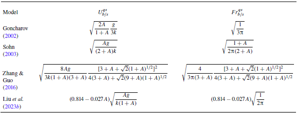
) for bubbles and spikes in different potential-flow models are summarised in table 2. The horizontal lines of
 $Fr_b^{qs}$
and
 $Fr_s^{qs}$
given by these potential-flow models are close to each other but consistently lower than the experimental values. This indicates that the rarefaction-driven bubbles and spikes achieve higher asymptotic growth rates compared with constant acceleration conditions. Figures 5(
 $a$
) and 5(
 $b$
) also include the theoretical predictions of
 $Fr_b$
and
 $Fr_s$
based on our model (2.24), in which the density derivative terms in (2.12)–(2.14) are set to zero. In other words, the model considers variable acceleration only. The predictions are lower than the experimental quasi-steady Froude numbers but approach predictions under constant acceleration. This is consistent with the previous numerical finding that when the flow is driven solely by variable acceleration, the quasi-steady Froude numbers converge to the theoretical values predicted under constant acceleration (Ramaprabhu et al. Reference Ramaprabhu, Karkhanis, Banerjee, Varshochi, Khan and Lawrie2016). Therefore, the higher quasi-steady Froude numbers in rarefaction-driven flows are attributed to the compressible effects resulting from time-dependent density, rather than variable acceleration.
Quasi-steady velocities (
 $U_{b/s}^{qs}$
) and Froude numbers (
 $Fr_{b/s}^{qs}$
) for bubbles and spikes obtained from different potential-flow models. The models of Goncharov (Reference Goncharov2002) and Sohn (Reference Sohn2003) are applicable only to bubbles, whereas the models of Zhang & Guo (Reference Zhang and Guo2016) and Liu et al. (Reference Liu, Zhang and Xiao2023b
) apply to both bubbles and spikes, with
 $A\gt 0$
corresponding to bubbles and
 $A\lt 0$
to spikes.

To account for the effect of time-dependent density, the finger growth rates obtained by (2.24), along with the acceleration and Atwood numbers in rarefaction-driven flows, are substituted into (4.4), and the time-dependent
 $Fr_b$
and
 $Fr_s$
are obtained. From figures 5(
 $a$
) and 5(
 $b$
), the model effectively captures the increase in Froude numbers in rarefaction-driven flows, which demonstrates the significance of the compressibility effect. Note that in the rarefaction field, the density decreases gradually from the wave head to its tail. As the interface moves toward the wave tail, the fluid penetrated by the bubbles and spikes becomes progressively lighter, thereby reducing the drag forces acting on the bubble tips and spike tips. Thus, the bubbles and spikes need to achieve higher asymptotic velocities to balance the drag and buoyancy forces. This results in larger Froude numbers in rarefaction-driven flows, compared with flows driven solely by constant or time-dependent acceleration.
4.3. Further validation across varied Atwood numbers
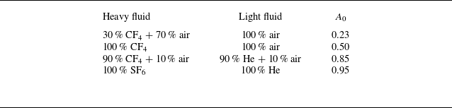
Since the late-time interface profile for lower Atwood number cases becomes increasingly indistinct in experimental schlieren imaging (Gao et al. Reference Gao, Guo, Zhai and Luo2024), numerical simulations are employed to assess the model’s applicability across different Atwood numbers. In the simulations, four different initial Atwood numbers,
 $A_0$
= 0.23, 0.50, 0.85 and 0.95, are generated by adjusting the species and concentrations of gases on either side of the interface. The specific gas combinations for these numerical cases are listed in table 3. The initial interface amplitude and wavelength for each numerical case are 2 and 60 mm, respectively. Other initial conditions are the same as those in the experiments. Note that the numerical case with
 $A_0$
= 0.85 has identical initial conditions compared with the experimental case 2-60.
Gas combinations and initial Atwood numbers for the numerical cases.

Comparison of amplitude growth for bubbles and spikes between numerical simulations and our model (2.24) at
 $A_0$
= 0.23 (
 $a$
), 0.50 (
 $b$
), 0.85 (
 $c$
) and 0.95 (
 $d$
). Experimental data of case 2-60 are included in panel (
 $c$
) for comparison.

The comparisons of finger growth at different Atwood numbers between the numerical results and the predictions of our model (2.24) as well as the Mikaelian’s model (4.1)–(4.2) are displayed in figure 6(
 $a$
–
 $d$
). The experimental data for case 2-60 are plotted in figure 6(
 $c$
) for comparison, showing good agreement with the numerical results. For low Atwood numbers (
 $A_0$
= 0.23), the Mikaelian model slightly overestimates the numerical bubble growth, while for high Atwood numbers (
 $A_0$
= 0.85 and 0.95), the Mikaelian model gives the same prediction as our model. Overall, our model provides excellent predictions of the numerical amplitude growth for both bubbles and spikes across different Atwood numbers.
The model (2.24) is also verified through the numerical results for a single-mode SF
 $_6$
/air interface (
 $A_0$
= 0.67) obtained from the 2-D Miranda simulations by Morgan et al. (Reference Morgan, Cabot, Greenough and Jacobs2018), as illustrated in figure 7. The comparison demonstrates that our model can also accurately capture the growth of both bubbles and spikes reported by Morgan et al. (Reference Morgan, Cabot, Greenough and Jacobs2018).
Figures 8(
 $a$
) and 8(
 $b$
) compare the temporal evolution of bubble (
 $\xi _b$
) and spike (
 $\xi _s$
) curvatures from numerical simulations against prediction of the model (2.22) at varying Atwood numbers (
 $A_0$
). The bubble curvature evolution shows minimal sensitivity to
 $A_0$
, with curvature trajectories converging to similar asymptotic values across cases. However, the spike asymptotic curvature increases with increasing
 $A_0$
. Notably, during the transition from initial to asymptotic states, the curvature growth rate varies non-monotonically with
 $A_0$
: the curvature growth rate for
 $A_0$
= 0.85 exceeds that for
 $A_0$
= 0.95. This anomaly arises from differences in gas composition (table 3): the
 $A_0$
= 0.85 case employs a mixture of 90 % CF4/10 % air as heavy fluid, generating stronger rarefaction waves compared with pure SF
 $_6$
(
 $A_0$
= 0.95) (Han & Yin Reference Han and Yin1993). Enhanced rarefaction amplifies finger growth rates, as shown in figures 6(
 $c$
) and 6(
 $d$
), which in turn accelerates curvature evolution. These trends are successfully captured by the model (2.22). In short, the model (2.22) captures both the
 $A_0$
-dependent asymptotic curvature of spikes and the non-monotonic growth behaviour of bubbles induced by rarefaction effects. This consistency confirms the model’s predictive capability across a broad range of
 $A_0$
.
Comparison of finger growth between the theoretical prediction from our model (2.24) and the numerical results of a single-mode SF
 $_6$
/air interface (
 $A_0$
= 0.67) from the 2-D Miranda simulations by Morgan et al. (Reference Morgan, Cabot, Greenough and Jacobs2018).

Comparison of curvature for bubbles (
 $a$
) and spikes (
 $b$
) between numerical simulations and our model (2.22) at different Atwood numbers.

5. Conclusion
Rayleigh–Taylor instability caused by rarefaction waves not only features variable acceleration but also incorporates time-dependent density, which introduce great challenges in predicting the finger growth behaviours. In this work, by extending Layzer’s potential-flow framework (Zhang & Guo Reference Zhang and Guo2016) to account for time-dependent acceleration and density, a theoretical model is developed to describe the 2-D amplitude growth of both bubbles and spikes. Relative to the previous models, the present model can evaluate the effect of time-dependent density on the finger growth, and can describe the growth behaviours of both bubbles and spikes in rarefaction-driven RTI flows. In addition, the time-dependent curvature of the finger tip as it evolves from its initial value to the quasi-steady value is quantified.
To validate the model, rarefaction-tube experiments on discontinuous single-mode interfaces with varying amplitude–wavelength combinations generated using the soap-film technique are carried out. In addition, numerical simulations with low, moderate and high Atwood numbers are conducted to further assess the model’s applicability across distinct density ratios. The results show that the present model can accurately capture the amplitude growth and curvature evolution of bubbles and spikes across various density ratios. The reliability of our model is also verified by the numerical results obtained from the 2-D Miranda simulations by Morgan et al. (Reference Morgan, Cabot, Greenough and Jacobs2018). Moreover, both the present model and experiments demonstrate that the continuous density reduction in rarefaction-driven flows causes larger asymptotic velocities of bubbles and spikes in the quasi-steady stage, leading to higher Froude numbers relative to those under constant or time-dependent acceleration. This is because the sustained density reduction in the rarefaction field decreases the drag forces acting on the bubble tips and spike tips. As a result, bubbles and spikes achieve larger asymptotic velocities to balance drag and buoyancy forces.
The current model focuses on 2-D, single-mode RTI configurations, however, its framework supports several natural extensions. First, extending the model to 3-D geometries or multi-mode perturbations would enable study of such phenomena as mode coupling and turbulent mixing. Second, the model’s input parameters, time-dependent acceleration and density, allow adaptation to arbitrary acceleration profiles and dynamic density evolution. Third, by neglecting density variations, the model simplifies to study RTI dominated by only variable acceleration, such as acceleration reversals (Aslangil, Lawrie & Banerjee Reference Aslangil, Lawrie and Banerjee2022; Pak et al. Reference Pak, Theriot, Aslangil, Lawrie and Banerjee2025).
Acknowledgements
The authors would like to thank Dr Z. Zhou for his help in numerical simulation and analysis.
Funding
This work was supported by the National Natural Science Foundation of China (Nos. 12302371, 12372281 and 12388101), the Youth Innovation Promotion Association CAS, the Strategic Priority Research Program of Chinese Academy of Sciences (No. XDB0620201) and the Fundamental Research Funds for the Central Universities (No. WK2090000048).
Declaration of interests
The authors report no conflict of interest.
Appendix A. Expressions for the rarefaction-induced acceleration and density
Recently, Gao et al. (Reference Gao, Guo, Zhai and Luo2024) derived the analytical solutions for the rarefaction-induced acceleration (
 $g_r$
) and the densities (
 $\rho _h$
and
 $\rho _l$
) of heavy and light fluids on either side of the interface. The expressions of
 $g_r$
,
 $\rho _h$
and
 $\rho _l$
can be expressed respectively as
 \begin{align} & \qquad\qquad\qquad g_r(t)=\zeta _1\theta _1t^{\theta _1-1}+\zeta _2\theta _2t^{\theta _2-1},\end{align}
 \begin{align} & \rho _h(t)=\rho _{h0}\left (1+\frac {\gamma _{h}-1}{2} \frac {u^\ast }{c_{h0}}\right )^{\frac {2}{\gamma _{h}-1}}\left (1-\frac {\gamma _{h}-1}{2} \frac {u_r-u^\ast }{c^\ast }\right )^{\frac {2}{\gamma _{h}-1}}, \\[-12pt] \nonumber\end{align}
 \begin{equation} \rho _l(t)=\rho _{l0}\left (1+\frac {\gamma _{l}-1}{2} \frac {u_r}{c_{l0}}\right )^{\frac {2}{\gamma _{l}-1}}, \end{equation}
with
 \begin{equation} \theta _{1,2}=\left (-1\pm \sqrt {1-\frac {4p_0 }{\rho _{l0}}\frac {2\gamma _{l}(\gamma _{l}-1)}{(\gamma _{l}+1)^2c_{l0}^2}}\right )/2. \end{equation}
Here,
 $p_0$
denote the initial flow pressure;
 $\rho _{h0}$
and
 $\rho _{l0}$
(
 $c_{h0}$
,
 $c_{l0}$
;
 $\gamma _{h}$
,
 $\gamma _{l}$
) denote the initial densities (sound speeds and adiabatic indices) for heavy and light fluids, respectively;
 $\zeta _1$
and
 $\zeta _2$
, dependent on the initial conditions, can be determined by solving geometric relations (see Gao et al. Reference Gao, Guo, Zhai and Luo2024);
 $u^\ast = (x_r/t-c_{h0} ) ({2}/{\gamma _h+1})$
and
 $c^\ast =c_{h0}-({\gamma _{h}-1}/{2})u^\ast$
; and
 $x_r$
and
 $u_r$
denote the rarefaction-induced interface displacement and velocity, respectively, with
 \begin{equation} x_r(t)=\frac {\zeta _1}{\theta _1+1}t^{\theta _1+1}+\frac {\zeta _2}{\theta _2+1}t^{\theta _2+1}-\frac {2}{\gamma -1}c_{l0}t+\kappa , \end{equation}
and
 \begin{equation} u_r(t)=\zeta _1t^{\theta _1}+\zeta _2t^{\theta _2} -\frac {2}{\gamma _l-1}c_{l0}. \end{equation}
Here,
 $\kappa$
in (A5) can be determined by solving geometric relations (Gao et al. Reference Gao, Guo, Zhai and Luo2024).
Appendix B. One-dimensional rarefaction-tube flow
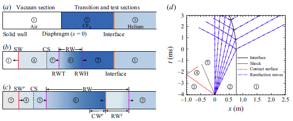
Distributions of flow regions in the rarefaction tube at different moments: (
 $a$
) the moment before the diaphragm rupture, (
 $b$
) the moment after the diaphragm rupture and (
 $c$
) the moment after the rarefaction waves reach the interface. Here, RWH and RWT denote the head and tail of the rarefaction waves, respectively; CS denotes the contact surface; and RW
 $^t$
and CW
 $^r$
denote the transmitted rarefaction waves and reflected compression waves, respectively. (
 $d$
) The
 $x$
–
 $t$
plot of the 1-D rarefaction-tube flow.

Figure 9(
 $a$
–
 $c$
) presents the distributions of flow regions at specific moments in the rarefaction tube. Before the diaphragm rupture, the diaphragm and the CF
 $_4$
/helium interface divide the flow fields into regions 1, 2 and 3, as shown in figure 9(
 $a$
). The sudden rupture of the diaphragm generates an upstream-travelling shock (SW), downstream-travelling rarefaction waves (RW) and a contact surface (CS) between these two waves, as depicted in figure 9(
 $b$
). The zones on either side of CS are designated as regions 4 and 5, with both velocities and pressures remaining constant across CS. The RW propagate downstream, transforming region 2 to region 6, characterised by time-dependent flow parameters. The interaction of RW with the CF
 $_4$
/helium interface generates downstream-moving transmitted rarefaction waves (RW
 $^t$
) and upstream-moving reflected compression waves (CW
 $^r$
), leading to the interface moving upstream continuously, as depicted in figure 9(
 $c$
). Figure 9(
 $d$
) shows the
 $x$
–
 $t$
diagram of the 1-D rarefaction-tube flow based on our experimental conditions. After the rarefaction waves impact, the interface undergoes variable acceleration motion. During the experimental duration (
 $t$
 $\approx$
0–3 ms), the shock reflected from the end wall does not arrive at the interface, thereby having no influence on the interface evolution.
In the experiments, the evolving interface must remain within the rarefaction region. This requires the rarefaction tail to move upstream along the vacuum section after the diaphragm rupture. The condition for the rarefaction tail moving upstream can be expressed as
 \begin{equation} v_{tl}=c_5-u_5 \lt 0, \end{equation}
where
 $v_{tl}$
denotes the velocity of the rarefaction tail, and
 $c_5$
and
 $u_5$
denote the sound speed and flow velocity in region 5, respectively. According to 1-D gas dynamics theory (Han & Yin Reference Han and Yin1993),
 $c_5$
and
 $u_5$
can be expressed respectively as
 \begin{align}& c_{5}=\sqrt {\frac {\gamma _5p_5}{\rho _5}}=\sqrt {\frac {\gamma _2p_2} {\rho _2^\ast }\left \{1+\frac {\gamma _2-1}{2}\left [\sqrt {\frac {\gamma _2\rho _1^\ast }{\gamma _1\rho _2^\ast }}\frac {M_s(\gamma _1+1)} {2(M_s^2-1)}-\frac {\gamma _2-1}{2}\right ]^{-1}\right \}^{\gamma _2}},\end{align}
 \begin{align} & \qquad\qquad\qquad\qquad\qquad u_{5}=\frac {2c_1}{\gamma _1+1} \left (M_s-\frac {1}{M_s}\right ),\end{align}
where
 $\gamma$
,
 $p$
and
 $\rho$
(or
 $\rho ^\ast$
) denote the adiabatic index, pressure and density, respectively, with the subscripts corresponding to the regions illustrated in figure 9; and
 $M_s$
denotes the shock Mach number, which can be obtained by numerically solving the following expression:
 \begin{equation} \frac {p_2}{p_1}=\left [1+\frac {2\gamma _1}{\gamma _1+1}(M^2_s-1)\right ]\left [1-\frac {\gamma _2-1} {\gamma _1+1}\frac {c_1}{c_2}\left (M_s-\frac {1}{M_s}\right )\right ]^{-\frac {2\gamma _2}{\gamma _2-1}}, \end{equation}
with
 $p_2/p_1$
denoting the initial pressure ratio of gases on either side of the diaphragm. Combining (B1)–(B4),
 $v_{tl}$
can be expressed as a function of
 $p_2/p_1$
. By numerically solving the relation between
 $v_{tl}$
and
 $p_2/p_1$
, the condition for
 $v_{tl}\lt 0$
is determined as
 $p_2/p_1$
 $\gt$
5.969. In our experiments, the diaphragm is broken at 10 kPa, resulting in
 $p_2/p_1$
= 10, ensuring that the rarefaction tail consistently moves upstream.
Appendix C. Numerical methods
The rarefaction–interface interactions are simulated by solving 2-D compressible multi-component Euler equations. The optimised six-point weighted compact nonlinear scheme (WCNS) with minimum dispersion and adaptive dissipation (Zhou et al. Reference Zhou, Ding, Huang and Luo2023b ) is used. Combined with the double-flux algorithm of Abgrall & Karni (Reference Abgrall and Karni2001), the optimised WCNS scheme is extended to multi-species flows, demonstrating a good capability in simulating RTI and shock-induced interface instabilities (Zhou et al. Reference Zhou, Ding, Cheng and Luo2023a , Reference Zhou, Ding, Huang and Luob , Reference Zhou, Ding and Cheng2024).
(
 $a$
) The computational domain used for the rarefaction–interface interaction. Numerical results of case 2–40 under different mesh sizes: (
 $b$
) density distribution along the symmetric line of the interface at
 $t$
= 911
 $\unicode {x03BC}$
s, and (
 $c$
) temporal variations of the perturbation amplitude. Experimental data of case 2-40 are included in panel (
 $c$
) for comparison.

The schematic of the computational domain is presented in figure 10(
 $a$
), where the virtual diaphragm is located at
 $x$
= 0, the initial interface at
 $x$
= 758.5 mm and the left and right boundaries of the domain at
 $x$
=
 $-$
700 and 1400 mm, respectively. The domain length is sufficiently large to prevent interference from reflected waves produced at the domain boundaries during the simulation. A pressure difference is initially applied across
 $x$
= 0, forming rarefaction waves that propagate in the positive direction along the
 $x$
-axis.
Four mesh sizes of 0.5, 0.4, 0.2 and 0.1 mm are adopted for grid convergence examination. The initial conditions for the numerical simulations match those of the experimental case 2-40. Figure 10(
 $b$
) shows the density distribution along the symmetry line of the interface at
 $t$
= 911
 $\unicode {x03BC}$
s, and figure 10(
 $c$
) shows the temporal variations of the perturbation amplitude. As the grid size decreases, both the density and amplitude curves converge, with similar results for mesh sizes of 0.2 and 0.1 mm. To balance computational cost and accuracy, a mesh size of 0.2 mm is selected in computations.
Comparison between the experimental (
 $a$
) and numerical (
 $b$
) schlieren images of interface evolution for a single-mode CF
 $_4$
/helium interface in case 2-40. Numbers denote time in
 $\unicode {x03BC}$
s.

The interface evolution in case 2-40 is compared between experimental and numerical results, as shown in figure 11. To maintain a discontinuous interface, a diffusion thickness of 0.5 mm is used in the simulations. This sharp interface introduces numerous small perturbations due to the Cartesian gridding. These small perturbations grow continuously under sustained energy injection from the rarefaction waves, triggering secondary RTI, as illustrated in figure 11(
 $b$
). Although the origins of the small perturbations differ between the simulation and the experiment, the interface evolution morphologies in figures 11(
 $a$
) and 11(
 $b$
) exhibit strong similarity. A quantitative comparison between the experimental and numerical results is presented in figure 10(
 $c$
), demonstrating good agreement.