2.1 Large Mach-number limit

In the strong-shock limit, $M\gg 1$ , shock dynamics provides the asymptotic relation

(2.10) $$\begin{eqnarray}q(A)=A^{-1/p}(\unicode[STIX]{x1D6FD},t),\end{eqnarray}$$

where

(2.11) $$\begin{eqnarray}p\equiv p(\unicode[STIX]{x1D6FE})=1+\frac{2}{\unicode[STIX]{x1D6FE}}+\sqrt{\frac{2\unicode[STIX]{x1D6FE}}{\unicode[STIX]{x1D6FE}-1}},\end{eqnarray}$$

$\unicode[STIX]{x1D6FE}$ being the (constant) ratio of specific heats, so that

(2.12) $$\begin{eqnarray}\frac{\unicode[STIX]{x2202}Z}{\unicode[STIX]{x2202}\unicode[STIX]{x1D70F}}=\text{i}\left(\frac{\unicode[STIX]{x2202}Z}{\unicode[STIX]{x2202}\unicode[STIX]{x1D6FD}}\frac{\unicode[STIX]{x2202}Z^{\ast }}{\unicode[STIX]{x2202}\unicode[STIX]{x1D6FD}}\right)^{-(p+1/2p)}\frac{\unicode[STIX]{x2202}Z}{\unicode[STIX]{x2202}\unicode[STIX]{x1D6FD}},\end{eqnarray}$$

where the variable transformation $\unicode[STIX]{x1D70F}=a_{0}M_{0}t$ scales the constants $M_{0},a_{0}$ out of the system. Strictly, $\unicode[STIX]{x1D70F}$ is space-like but we will refer to it as a re-scaled time for convenience of interpretation. We study this formulation because it is relatively simpler than (2.9) and allows for a straightforward Fourier representation.

Equation (2.12) describes the evolution in time of the entire shock. It can be written in terms of the perturbation $z(\unicode[STIX]{x1D6FD},\unicode[STIX]{x1D70F})$ on the motion of the flat shock, $Z_{0}(\unicode[STIX]{x1D6FD},\unicode[STIX]{x1D70F})=\unicode[STIX]{x1D6FD}+\text{i}\unicode[STIX]{x1D70F}$ , by using (2.2) and (2.3). Using the shorthand $D=\unicode[STIX]{x2202}/\unicode[STIX]{x2202}\unicode[STIX]{x1D6FD}$ we obtain

(2.13) $$\begin{eqnarray}\frac{\unicode[STIX]{x2202}z}{\unicode[STIX]{x2202}\unicode[STIX]{x1D70F}}+\text{i}=\text{i}[(1+Dz)(1+Dz^{\ast })]^{-(p+1/2p)}(1+Dz),\end{eqnarray}$$

noting that since $\unicode[STIX]{x1D6FD}$ is real, $Dz^{\ast }=D(z^{\ast })=(Dz)^{\ast }$ . Equation (2.13) will be the main focus of this study.

To leading order (2.13) is also valid for strong, fast MHD shocks which are parallel to an applied (uniform) magnetic field ahead of the shock in the mean. This corresponds to MHD shocks where the magnetosonic Mach number $M_{f}=Ma_{0}/c_{f0}\gg 1$ , where $c_{f0}$ is the magnetosonic speed for a parallel field ahead of the shock. This is because $M_{f}\gg 1$ implies $M\gg 1$ and it is shown in appendix A that in this limit the gas-dynamic result (2.10) is recovered with a small correction. This case is presented briefly in § 7. The weak-shock MHD case ( $M_{f}-1\ll 1$ ) is not considered here.

2.2 Small Mach-number limit

When the gas-dynamic shock is weak, that is when $M-1\ll 1$ , then the asymptotic relation between $M$ and $A$ is

(2.14) $$\begin{eqnarray}\frac{(M-1)^{2}}{(M_{0}-1)^{2}}\sim \frac{A_{0}}{A}.\end{eqnarray}$$

By substitution directly into (2.4), we have

(2.15) $$\begin{eqnarray}\frac{\unicode[STIX]{x2202}Z}{\unicode[STIX]{x2202}t}=\text{i}a_{0}\left[(M_{0}-1)\left(\frac{\unicode[STIX]{x2202}Z}{\unicode[STIX]{x2202}\unicode[STIX]{x1D6FD}}\frac{\unicode[STIX]{x2202}Z^{\ast }}{\unicode[STIX]{x2202}\unicode[STIX]{x1D6FD}}\right)^{-1/4}+1\right]\frac{\unicode[STIX]{x2202}Z}{\unicode[STIX]{x2202}\unicode[STIX]{x1D6FD}}\left(\frac{\unicode[STIX]{x2202}Z}{\unicode[STIX]{x2202}\unicode[STIX]{x1D6FD}}\frac{\unicode[STIX]{x2202}Z^{\ast }}{\unicode[STIX]{x2202}\unicode[STIX]{x1D6FD}}\right)^{-1/2}.\end{eqnarray}$$

This equation may be treated by the same substitution of $z=Z-(\unicode[STIX]{x1D6FD}+\text{i}a_{0}M_{0}\,t)$ as for (2.13).

5.1 Development of solution form

The equations (4.7) form a system of linear, inhomogeneous ODEs, except for the case $|m|=1$ which is homogeneous. For a given $m>0$ , we have the positive and negative modes given by

(5.1) $$\begin{eqnarray}\displaystyle & \displaystyle \frac{\text{d}R_{m}}{\text{d}\unicode[STIX]{x1D70F}}=-mR_{m}-mb_{1}(R_{m}+R_{-m}^{\ast })+\text{i}f_{m}, & \displaystyle\end{eqnarray}$$

(5.2) $$\begin{eqnarray}\displaystyle & \displaystyle \frac{\text{d}R_{-m}}{\text{d}\unicode[STIX]{x1D70F}}=mR_{-m}+mb_{1}(R_{-m}+R_{m}^{\ast })+\text{i}f_{-m}, & \displaystyle\end{eqnarray}$$

dropping the tildes for convenience. $f_{\pm m}$ is a forcing term depending only on the lower mode solutions $R_{j}$ , $j<m$ . Solving sequentially $|m|=1,2,3,\ldots$ the forcing term is therefore always known in terms of the lower mode solutions, and hence in principle all the solutions may be produced recursively. However, we desire the behaviour of the $R_{m}$ for $m\gg |1|$ which is unfeasible to produce in this manner. But if the general form of $R_{m}(\unicode[STIX]{x1D70F})$ can be deduced, then it is possible to determine the behaviour of these coefficients asymptotically without the need for recursive solutions. We do this as follows. Compose (5.1)–(5.2) into a single second-order ODE,

(5.3) $$\begin{eqnarray}\frac{\text{d}^{2}R_{m}}{\text{d}\unicode[STIX]{x1D70F}}+b_{1}m^{2}\left(b_{1}-\frac{(b_{1}+1)^{2}}{b_{1}}\right)R_{m}=\text{i}\left(\frac{\text{d}f_{m}}{\text{d}\unicode[STIX]{x1D70F}}+b_{1}mf_{-m}^{\ast }-m(b_{1}+1)f_{m}\right).\end{eqnarray}$$

For $m=1$ , the forcing terms are $f_{m}=f_{-m}^{\ast }=0$ so that (5.3) is homogeneous and we have the solution

(5.4) $$\begin{eqnarray}\left.\begin{array}{@{}c@{}}R_{1}(\unicode[STIX]{x1D70F})=C_{+}\text{e}^{\sqrt{1+2b_{1}}\unicode[STIX]{x1D70F}}+C_{-}\text{e}^{-\sqrt{1+2b_{1}}\unicode[STIX]{x1D70F}},\\ R_{-1}^{\ast }(\unicode[STIX]{x1D70F})=C_{+}M_{+}\text{e}^{\sqrt{1+2b_{1}}\unicode[STIX]{x1D70F}}+C_{-}M_{-}\text{e}^{-\sqrt{1+2b_{1}}\unicode[STIX]{x1D70F}},\end{array}\right\}\end{eqnarray}$$

where

(5.5a,b ) $$\begin{eqnarray}M_{+}=-\frac{(1+b_{1}+\sqrt{1+2b_{1}})}{b_{1}},\quad M_{-}=-\frac{(1+b_{1}-\sqrt{1+2b_{1}})}{b_{1}},\end{eqnarray}$$

and the complex constants $C_{\pm }$ are determined from the IC constant $\unicode[STIX]{x1D70E}$ ,

(5.6) $$\begin{eqnarray}C_{\pm }=\pm \frac{\text{i}(1+b_{1}-\unicode[STIX]{x1D70E}^{\ast }b_{1}\mp \sqrt{1+2b_{1}})}{4\sqrt{1+2b_{1}}}.\end{eqnarray}$$

Since $1+2b_{1}=-1/p(\unicode[STIX]{x1D6FE})$ , and $p(\unicode[STIX]{x1D6FE})>0$ for $\unicode[STIX]{x1D6FE}>1$ (as for ideal gases) for any reasonable choice of $\unicode[STIX]{x1D6FE}$ (see § 6), the exponentials in (5.4) are purely oscillatory. Note also that $M_{\pm }$ are complex numbers with unity magnitude, so their effect in the $-m$ solution is that of a time-phase shift to each term.

The forcing term of (5.3) for $m=2$ is

(5.7) $$\begin{eqnarray}\displaystyle F_{2} & = & \displaystyle {\displaystyle \frac{\text{d}f_{2}}{\text{d}\unicode[STIX]{x1D70F}}}+2b_{1}\,f_{-2}^{\ast }-2(b_{1}+1)f_{2}\end{eqnarray}$$

(5.8) $$\begin{eqnarray}\displaystyle & = & \displaystyle 2(K_{+}C_{+}^{2}\text{e}^{2\sqrt{1+2b_{1}}\unicode[STIX]{x1D70F}}+K_{-}C_{-}^{2}\text{e}^{-2\sqrt{1+2b_{1}}\unicode[STIX]{x1D70F}})+O(1),\end{eqnarray}$$

where

(5.9) $$\begin{eqnarray}\displaystyle K_{+} & = & \displaystyle (1-M_{+}^{2})b_{1}^{2}+(2M_{+}+1)b_{1}(1-\sqrt{1+2b_{1}})\end{eqnarray}$$

(5.10) $$\begin{eqnarray}\displaystyle & & \displaystyle +\,(M_{+}+1)^{2}(1-\sqrt{1+2b_{1}})b_{2},\end{eqnarray}$$

(5.11) $$\begin{eqnarray}\displaystyle K_{-} & = & \displaystyle (1-M_{-}^{2})b_{1}^{2}+(2M_{-}+1)b_{1}(1+\sqrt{1+2b_{1}})\end{eqnarray}$$

(5.12) $$\begin{eqnarray}\displaystyle & & \displaystyle +\,(M_{-}+1)^{2}(1+\sqrt{1+2b_{1}})b_{2},\end{eqnarray}$$

and in fact $K_{-}=K_{+}^{\ast }$ , and we have the corresponding particular solution

(5.13) $$\begin{eqnarray}\left.\begin{array}{@{}c@{}}R_{2}(\unicode[STIX]{x1D70F})={\displaystyle \frac{\text{i}\unicode[STIX]{x1D70F}}{2\sqrt{1+2b_{1}}}}(C_{+}^{2}K_{+}\text{e}^{2\sqrt{1+2b_{1}}\unicode[STIX]{x1D70F}}-C_{-}^{2}K_{-}\text{e}^{-2\sqrt{1+2b_{1}}\unicode[STIX]{x1D70F}})+O(1),\\ R_{-2}^{\ast }(\unicode[STIX]{x1D70F})={\displaystyle \frac{\text{i}\unicode[STIX]{x1D70F}}{2\sqrt{1+2b_{1}}}}(C_{+}^{2}K_{+}M_{+}\text{e}^{2\sqrt{1+2b_{1}}\unicode[STIX]{x1D70F}}-C_{-}^{2}K_{-}M_{-}\text{e}^{-2\sqrt{1+2b_{1}}\unicode[STIX]{x1D70F}})+O(1),\end{array}\right\}\end{eqnarray}$$

where the homogeneous part of the solution is held in the $O(1)$ term since it is dominated by the $O(\unicode[STIX]{x1D70F})$ particular integral. We note in passing this implies that the initial conditions to the $m=2$ mode do not contribute to its growth in the leading order, subject to the constraints specified in § 4. Comparison of (5.4) with (5.13) suggests the following ansatz for $R_{m}$ ,

(5.14) $$\begin{eqnarray}\displaystyle & \displaystyle R_{m}(\unicode[STIX]{x1D70F})=\unicode[STIX]{x1D70F}^{m-1}\left[C_{+}^{m}\unicode[STIX]{x1D706}_{m}^{+}\text{e}^{m\sqrt{1+2b_{1}}\unicode[STIX]{x1D70F}}+C_{-}^{m}\unicode[STIX]{x1D706}_{m}^{-}\text{e}^{-m\sqrt{1+2b_{1}}\unicode[STIX]{x1D70F}}\right]+O(\unicode[STIX]{x1D70F}^{m-2}), & \displaystyle\end{eqnarray}$$

(5.15) $$\begin{eqnarray}\displaystyle & \displaystyle R_{-m}^{\ast }(\unicode[STIX]{x1D70F})=\unicode[STIX]{x1D70F}^{m-1}\left[C_{+}^{m}M_{+}\unicode[STIX]{x1D706}_{m}^{+}\text{e}^{m\sqrt{1+2b_{1}}\unicode[STIX]{x1D70F}}+C_{-}^{m}M_{-}\unicode[STIX]{x1D706}_{m}^{-}\text{e}^{-m\sqrt{1+2b_{1}}\unicode[STIX]{x1D70F}}\right]+O(\unicode[STIX]{x1D70F}^{m-2}), & \displaystyle\end{eqnarray}$$

so that if the behaviour of $\unicode[STIX]{x1D706}_{m}$ for large $m$ can be determined, then the leading-order asymptotic behaviour of the coefficients will be established.

5.2 Recursion relation for coefficients

The forcing terms are

(5.16) $$\begin{eqnarray}\displaystyle f_{m}(\unicode[STIX]{x1D70F}) & = & \displaystyle -\mathop{\sum }_{r_{1}+r_{2}=m}r_{1}r_{2} (\!b_{1}[R_{r_{1}}R_{-r_{2}}^{\ast }+R_{r_{1}}\{R_{r_{2}}+R_{-r_{2}}^{\ast }\}]\nonumber\\ \displaystyle & & \displaystyle +\,b_{2}[R_{r_{1}}+R_{-r_{1}}^{\ast }][R_{r_{2}}+R_{-r_{2}}^{\ast }])+\cdots \,,\end{eqnarray}$$

(5.17) $$\begin{eqnarray}\displaystyle f_{-m}^{\ast }(\unicode[STIX]{x1D70F}) & = & \displaystyle -\mathop{\sum }_{r_{1}+r_{2}=m}r_{1}r_{2} (\!b_{1}[R_{-r_{1}}^{\ast }R_{r_{2}}+R_{-r_{1}}^{\ast }\{R_{r_{2}}+R_{-r_{2}}^{\ast }\}]\nonumber\\ \displaystyle & & \displaystyle +\,b_{2}[R_{r_{1}}+R_{-r_{1}}^{\ast }][R_{r_{2}}+R_{-r_{2}}^{\ast }])+\cdots \,,\end{eqnarray}$$

(5.18) $$\begin{eqnarray}\displaystyle F_{m}(\unicode[STIX]{x1D70F}) & = & \displaystyle \frac{\text{d}f_{m}}{\text{d}\unicode[STIX]{x1D70F}}+mb_{1}\,f_{-m}^{\ast }-m(b_{1}+1)f_{m},\end{eqnarray}$$

which can be written more compactly as

(5.19) $$\begin{eqnarray}F_{m}=\mathop{\sum }_{s=2}^{m}\left[\unicode[STIX]{x1D70F}^{s-2}\mathop{\sum }_{q=0}^{m/2}\{\unicode[STIX]{x1D6E4}_{s}^{(q,+)}\text{e}^{(m-2q)\sqrt{1+2b_{1}}\unicode[STIX]{x1D70F}}+\unicode[STIX]{x1D6E4}_{s}^{(q,-)}\text{e}^{-(m-2q)\sqrt{1+2b_{1}}\unicode[STIX]{x1D70F}}\}\right].\end{eqnarray}$$

The upper bound on the second sum of (5.19) is taken as $(m-1)/2$ if $m$ is odd. The coefficients $\unicode[STIX]{x1D6E4}_{s}^{(q,\pm )}$ (the superscripts and subscripts signify labels) can be determined explicitly from the lower mode solutions. It can be shown, first, that only the leading-order term $s=m$ contributes to the leading-order term of the solution $R_{m}$ , and second, that within this term the only leading-order contributor is the $q=0$ subterm. The $s=m$ term corresponds to the second-order convolutions in the forcing term, thus justifying our earlier truncation to those terms. Now after identifying the constants $\unicode[STIX]{x1D6E4}_{m}^{(0,\pm )}$ by comparison with (5.18) and substituting in the form of the ansatz, after some algebra we obtain

(5.20) $$\begin{eqnarray}\displaystyle & \displaystyle \unicode[STIX]{x1D6E4}_{m}^{(0,+)}=mC_{+}^{m}K_{+}\mathop{\sum }_{r_{1}+r_{2}=m}r_{1}r_{2}\unicode[STIX]{x1D706}_{r_{1}}^{+}\unicode[STIX]{x1D706}_{r_{2}}^{+}, & \displaystyle\end{eqnarray}$$

(5.21) $$\begin{eqnarray}\displaystyle & \displaystyle \unicode[STIX]{x1D6E4}_{m}^{(0,-)}=mC_{-}^{m}K_{-}\mathop{\sum }_{r_{1}+r_{2}=m}r_{1}r_{2}\unicode[STIX]{x1D706}_{r_{2}}^{-}\unicode[STIX]{x1D706}_{r_{2}}^{-}, & \displaystyle\end{eqnarray}$$

and using variation of parameters to solve for $R_{m}$ gives

(5.22) $$\begin{eqnarray}\left.\begin{array}{@{}c@{}}\unicode[STIX]{x1D706}_{m}^{+}={\displaystyle \frac{\text{i}K_{+}}{2(m-1)\sqrt{1+2b_{1}}}}\displaystyle \mathop{\sum }_{r_{1}+r_{2}=m}r_{1}r_{2}\unicode[STIX]{x1D706}_{r_{1}}^{+}\unicode[STIX]{x1D706}_{r_{2}}^{+},\\ \unicode[STIX]{x1D706}_{m}^{-}={\displaystyle \frac{(\text{i}K_{+})^{\ast }}{2(m-1)\sqrt{1+2b_{1}}}}\displaystyle \mathop{\sum }_{r_{1}+r_{2}=m}r_{1}r_{2}\unicode[STIX]{x1D706}_{r_{1}}^{-}\unicode[STIX]{x1D706}_{r_{2}}^{-}.\end{array}\right\}\end{eqnarray}$$

This proves the ansatz by induction since it holds for the cases $m=1,2$ with $\unicode[STIX]{x1D706}_{1}^{\pm }=1$ , and (5.22) shows that if the $(m-1)$ th solution follows the ansatz then the $m$ th must as well.

5.3 Asymptotic behaviour

Equation (5.22) is a recursion relation for the $\unicode[STIX]{x1D706}_{m}^{\pm }$ but still not enough to determine analytically their asymptotic behaviour. For this we utilize the generating-function method of Moore (Reference Moore1979) for the amplitudes,

(5.23) $$\begin{eqnarray}g(x)=\mathop{\sum }_{m=1}^{\infty }|\unicode[STIX]{x1D706}_{m}|x^{m},\end{eqnarray}$$

over $x$ complex. The $\pm$ -superscript is omitted since (5.22) implies $|\unicode[STIX]{x1D706}_{m}^{+}|=|\unicode[STIX]{x1D706}_{m}^{-}|$ . Likewise, $|K_{+}|=|K_{-}|$ . Given (5.22), (5.23) satisfies the ODE

(5.24) $$\begin{eqnarray}\frac{\text{d}}{\text{d}x}\left(\frac{g(x)}{x}\right)=\frac{K_{B}}{2}\left(\frac{\text{d}g}{\text{d}x}\right)^{2},\end{eqnarray}$$

where $K_{B}=\text{i}|K_{\pm }|/\sqrt{1+2b_{1}}$ . Note that this ODE is similar in form to equation (3.8) of Moore (Reference Moore1979). This is because in both studies the quadratic in the system of inhomogeneous equations dominates the forcing term, leading to a recursion relation with the form of (5.22). Since $|\unicode[STIX]{x1D706}_{1}|=1$ there is the initial condition

(5.25) $$\begin{eqnarray}g^{\prime }(0)=1,\end{eqnarray}$$

giving the following solution to (5.24),

(5.26) $$\begin{eqnarray}g(x)=-\frac{2W(-xK_{B})+W^{2}(-xK_{B})}{2K_{B}},\end{eqnarray}$$

where $W(x)$ is the principal branch of the Lambert $W$ -function. Now $g(x)$ has a singularity in its derivative at $x_{c}=-(K_{B}e)^{-1}$ , but is analytic everywhere else on the circle in complex $x$ of radius $|x_{c}|$ . Recall that we seek the behaviour of $|\unicode[STIX]{x1D706}_{m}|$ as $m\rightarrow \infty$ . For this we use Darboux’s method (Olver Reference Olver1974). We seek a comparison function $f(x)$ which is analytic in some disc around $x_{c}$ , for which $g(x)-f(x)$ is continuous in that disc, and whose Laurent series expansion coefficients have known asymptotic behaviour. Then, the coefficients of the $g(x)$ generating function behave asymptotically like those of the $f(x)$ Laurent series. This comparison function is constructed as follows: $g(x)$ has a Laurent series expansion around $x_{c}$ ,

(5.27) $$\begin{eqnarray}g(x)\simeq \frac{1}{2K_{B}}-\frac{1-xK_{B}e}{K_{B}}+\frac{2\sqrt{2}(1-xK_{B}e)^{3/2}}{3K_{B}}+\cdots \,.\end{eqnarray}$$

The third term dominates singular behaviour in the derivative, and we identify it as $f(x)$ , satisfying the requirements and having an expansion

(5.28) $$\begin{eqnarray}f(x)=\frac{2\sqrt{2}(1-exK_{B})^{3/2}}{3K_{B}}=\mathop{\sum }_{m=0}^{\infty }a_{m}x^{m},\end{eqnarray}$$

with Darboux’s method concluding via the binomial theorem asymptotically,

(5.29) $$\begin{eqnarray}|\unicode[STIX]{x1D706}_{m}|\sim a_{m}\simeq \frac{1}{\sqrt{2\unicode[STIX]{x03C0}}}K_{B}^{m+1}\text{e}^{m}m^{-5/2}.\end{eqnarray}$$

Hence we have the asymptotic form of the shock perturbation Fourier coefficients to leading order:

(5.30) $$\begin{eqnarray}\displaystyle R_{m}(\unicode[STIX]{x1D70F}) & = & \displaystyle \text{i}\unicode[STIX]{x1D70F}^{m-1}K_{B}^{m+1}\text{e}^{m}m^{-5/2}\nonumber\\ \displaystyle & & \displaystyle \times (|C_{+}^{m}|\text{e}^{m\sqrt{1+2b_{1}}\unicode[STIX]{x1D70F}+\text{i}Q_{+}}+|C_{-}^{m}|\text{e}^{-m\sqrt{1+2b_{1}}\unicode[STIX]{x1D70F}+\text{i}Q_{-}})+O(\unicode[STIX]{x1D70F}^{m-1}),\end{eqnarray}$$

(5.31) $$\begin{eqnarray}\displaystyle R_{-m}^{\ast }(\unicode[STIX]{x1D70F}) & = & \displaystyle \text{i}\unicode[STIX]{x1D70F}^{m-1}K_{B}^{m+1}\text{e}^{m}m^{-5/2}\nonumber\\ \displaystyle & & \displaystyle \times (|C_{+}^{m}|M_{+}\text{e}^{m\sqrt{1+2b_{1}}\unicode[STIX]{x1D70F}+\text{i}Q_{+}}+|C_{-}^{m}|M_{-}\text{e}^{-m\sqrt{1+2b_{1}}\unicode[STIX]{x1D70F}+\text{i}Q_{-}})+O(\unicode[STIX]{x1D70F}^{m-1}),\qquad\end{eqnarray}$$

where $Q_{\pm }=\arg (\unicode[STIX]{x1D706}_{m}^{\pm }C_{\pm }^{m})$ . The generating function does not yield $\arg \unicode[STIX]{x1D706}_{m}^{\pm }$ but this is not important since its only effect is a time-phase shift to the oscillating part of $R_{m}$ . By definition of $R_{m}$ , we then have

(5.32) $$\begin{eqnarray}\displaystyle \hat{z}_{m}(\unicode[STIX]{x1D70F}) & = & \displaystyle \frac{\text{i}K_{B}m^{-5/2}}{\unicode[STIX]{x1D70F}}\exp (m(1+\log [\unicode[STIX]{x1D70F}K_{B}|C_{+}|\unicode[STIX]{x1D716}]))\{\text{e}^{m\sqrt{1+2b_{1}}\unicode[STIX]{x1D70F}+\text{i}Q_{+}}\}\nonumber\\ \displaystyle & & \displaystyle +\,\frac{\text{i}K_{B}m^{-5/2}}{\unicode[STIX]{x1D70F}}\exp (m(1+\log [\unicode[STIX]{x1D70F}K_{B}|C_{-}|\unicode[STIX]{x1D716}]))\{\text{e}^{-m\sqrt{1+2b_{1}}\unicode[STIX]{x1D70F}+\text{i}Q_{-}}\}\nonumber\\ \displaystyle & & \displaystyle +\,O(\unicode[STIX]{x1D716}^{m}\unicode[STIX]{x1D70F}^{m-1})+O(\unicode[STIX]{x1D716}^{m+1}\unicode[STIX]{x1D719}(\unicode[STIX]{x1D70F})),\end{eqnarray}$$

for $m>0$ , and similarly for $z_{-m}$ recalling that $|M_{+}|=|M_{-}|=1$ . We remark that the above analysis does not explicitly consider the $m=0$ mode. The highest-order contribution to the $m=0$ mode comes from second-order convolution of the $|m|=1$ terms, and so is an oscillatory function with $O(\unicode[STIX]{x1D716}^{2})$ . However it has no effect on any coefficients $m\neq 0$ because of the form of the forcing function.

5.4 Time to singularity formation

Our approach contains the combination of truncation with asymptotic analysis of the truncated system. We cannot justify this formally. Indeed, the order term involving $\unicode[STIX]{x1D719}(\unicode[STIX]{x1D70F})$ in (5.32) comes from the higher-order subsystems for $R_{m,j},j\neq 0$ , which have been neglected in this analysis. Therefore, in writing (5.32) we assume without proof that the unknown time dependence $\unicode[STIX]{x1D719}(\unicode[STIX]{x1D70F})$ is not so large that the first term ceases to be leading order. As noted by Moore (Reference Moore1979) for vortex-sheet evolution, ‘the possibility that the expansion is not uniformly valid as $m$ goes to infinity cannot be ruled out …the conclusions drawn here must remain merely plausible’. But such a non-uniformity would imply that $\hat{z}_{m}$ is greater than $O(\unicode[STIX]{x1D716}^{m})$ which is implausible in light of the reasoning in § 4. Thus, although we do not prove that the assumptions made in § 4 are correct, they are consistent with the neglect of $\unicode[STIX]{x1D719}(\unicode[STIX]{x1D70F})$ . In § 9 we will discuss the numerical evidence further supporting this assumption. There are two leading-order terms in (5.32). In each, the quantity in curled brackets is purely oscillatory, and the amplitude is controlled by the real exponent and the factor $m^{-5/2}$ . Therefore, the shock profile remains analytic for as long as

(5.33) $$\begin{eqnarray}1+\log [\unicode[STIX]{x1D70F}K_{B}C\unicode[STIX]{x1D716}]<0,\end{eqnarray}$$

where $C=\max (|C_{+}|,|C_{-}|)$ , implying that a singularity forms in the geometry of the shock at the critical time,

(5.34) $$\begin{eqnarray}\unicode[STIX]{x1D70F}_{c}=\frac{\text{e}^{-1}}{K_{B}C\unicode[STIX]{x1D716}},\end{eqnarray}$$

corresponding to whichever of the two leading terms in (5.32) first loses exponential decay. Using the definition of $\unicode[STIX]{x1D70F}$ and $K_{B}$ ,

(5.35) $$\begin{eqnarray}t_{c}=\frac{\text{e}^{-1}|\sqrt{1+2b_{1}}|}{M_{0}a_{0}|K_{\pm }|C\unicode[STIX]{x1D716}}.\end{eqnarray}$$

The constants $K_{+},K_{-}$ are given by (5.10), (5.11), themselves depending on $M_{\pm }$ given by (5.5) and $b_{1},b_{2}$ given by (3.3) by setting $k=1,2$ . These constants depend on Whitham’s exponent $p(\unicode[STIX]{x1D6FE})$ calculated by (2.11), and for comparisons made here we use a specific heat ratio $\unicode[STIX]{x1D6FE}=5/3$ . The constants $C_{+},C_{-}$ used in determining $C$ are given by (5.6) and contain the effect of the IC through the choice of $\unicode[STIX]{x1D70E}$ . Note that $C=|C_{+}|$ for $\text{Im}(\unicode[STIX]{x1D70E})\geqslant 0$ and $C=|C_{-}|$ for $\text{Im}(\unicode[STIX]{x1D70E})\leqslant 0$ , and hence for real $\unicode[STIX]{x1D70E}$ , $C=|C_{+}|=|C_{-}|$ .

This completes the analysis for strong shocks. At time $t_{c}$ , the Fourier coefficients cease to decay exponentially with mode number and hence analyticity is lost, or equivalently a singularity has formed in the shock geometry. Equation (5.35) suggests, firstly, that the formation time of the singularity occurs inversely proportional to amplitude. As implied by § 6 the form of this dependence is not restricted to the strong-shock limit, but the constant of proportionality in (5.34) is for this limit only. Singularity formation in a time that goes as $\unicode[STIX]{x1D716}^{-1}$ is in agreement with the numerical results and theoretical sketch provided in Mostert et al. (Reference Mostert, Pullin, Samtaney and Wheatley2017) for the gas-dynamic shock. We note in passing that this dependence is quite distinct from the result of Moore (Reference Moore1979) which predicts $t_{c}\propto \log \unicode[STIX]{x1D716}$ (with $\unicode[STIX]{x1D716}$ defined as in the present case). This difference arises because Moore’s form for the Fourier coefficients involves a factor $e^{mt}$ associated with perturbation amplitude growth for the vortex sheet, rather than the oscillatory behaviour of the propagating shock seen presently.

For the strong-shock limit, the constant is inversely proportional to the unperturbed shock speed $a_{0}M_{0}$ , directly proportional to the shock oscillation fundamental frequency $\unicode[STIX]{x1D714}_{0}=\text{Im}(\sqrt{1+2b_{1}})$ and in general is a function of $\unicode[STIX]{x1D6FE}$ and the initial condition via the constants $K_{\pm }$ and $C_{\pm }$ . The dependency on $\unicode[STIX]{x1D6FE}$ ultimately comes in through $b_{1},b_{2}$ , which, in the strong-shock limit, depend on Whitham’s exponent $p(\unicode[STIX]{x1D6FE})$ . 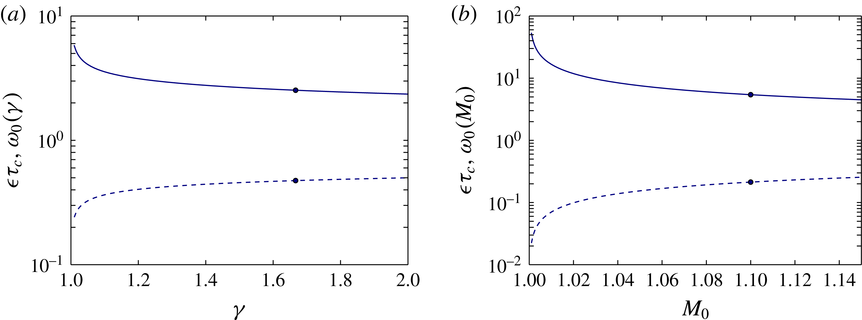Some features of these dependencies are discussed in figure 1, in § 6.1.

The algebraic decay rate of $m^{-5/2}$ in (5.32) indicates a loss of analyticity in the shock shape. At this stage the nature of the implied singularity at $t=t_{c}$ is not apparent. We might identify this with the formation of a shock–shock, if it were a discontinuity in slope, but this is not consistent with an $m^{-5/2}$ decay in Fourier coefficients. This is considered further in § 8.2, where the character of the singularity is discussed, and also in § 9. Lastly, equation (5.32) (and the leading-order solution to the first Fourier mode) asserts that the shock perturbations oscillate with a fundamental frequency $\text{Im}(\sqrt{1+2b_{1}})$ in time. The higher Fourier mode coefficients oscillate at a harmonic of this frequency, superimposed on polynomial growth in time.

6.1 Small Mach-number limit

On defining

(6.1) $$\begin{eqnarray}P(\unicode[STIX]{x1D6FD},\unicode[STIX]{x1D70E})=\mathop{\sum }_{k=1}^{\infty }c_{k}(\unicode[STIX]{x1D70E})(Dz+Dz^{\ast }+DzDz^{\ast })^{k},\quad c_{k}(\unicode[STIX]{x1D70E})=\binom{\unicode[STIX]{x1D70E}}{k},\end{eqnarray}$$

equation (2.15) becomes

(6.2) $$\begin{eqnarray}\text{i}a_{0}M_{0}+\frac{\unicode[STIX]{x2202}z}{\unicode[STIX]{x2202}t}=\text{i}a_{0}\left[(M_{0}-1)\left\{1+P\left(\unicode[STIX]{x1D6FD},-\frac{1}{4}\right)\right\}+1\right](1+Dz)\left\{1+P\left(\unicode[STIX]{x1D6FD},-\frac{1}{2}\right)\right\}.\end{eqnarray}$$

Retaining up to quadratic terms as in the previous analysis, this may be written (suppressing $\unicode[STIX]{x1D6FD}$ dependence for brevity)

(6.3) $$\begin{eqnarray}\displaystyle \frac{\unicode[STIX]{x2202}z}{\unicode[STIX]{x2202}t} & \simeq & \displaystyle \text{i}a_{0}\left[M_{0}\left\{P_{2}\left(-\frac{1}{4}\right)+P_{2}\left(-\frac{1}{2}\right)+Dz\right\}-P_{2}\left(-\frac{1}{4}\right)\right.\nonumber\\ \displaystyle & & \displaystyle +\,(M_{0}-1)\left\{\left[P_{1}\left(-\frac{1}{4}\right)+P_{1}\left(-\frac{1}{2}\right)\right]Dz+P_{1}\left(-\frac{1}{2}\right)P_{1}\left(-\frac{1}{4}\right)\right\}\nonumber\\ \displaystyle & & \displaystyle +\left.P_{1}\left(-\frac{1}{2}\right)Dz\right],\end{eqnarray}$$

where the $P_{k}(\unicode[STIX]{x1D70E})$ denote partial sums of $k$ terms. Define

(6.4) $$\begin{eqnarray}\displaystyle Q(\unicode[STIX]{x1D6FD},\unicode[STIX]{x1D70E}_{1},\unicode[STIX]{x1D70E}_{2}) & = & \displaystyle P(\unicode[STIX]{x1D6FD},\unicode[STIX]{x1D70E}_{1})+P(\unicode[STIX]{x1D6FD},\unicode[STIX]{x1D70E}_{2})\nonumber\\ \displaystyle & = & \displaystyle \mathop{\sum }_{k=1}^{\infty }(c_{k}(\unicode[STIX]{x1D70E}_{1})+c_{k}(\unicode[STIX]{x1D70E}_{2}))(Dz+Dz^{\ast }+DzDz^{\ast })^{k}\end{eqnarray}$$

(6.5) $$\begin{eqnarray}\displaystyle N_{1}(\unicode[STIX]{x1D6FD},\unicode[STIX]{x1D70E}_{1},\unicode[STIX]{x1D70E}_{2}) & = & \displaystyle P_{1}(\unicode[STIX]{x1D6FD},\unicode[STIX]{x1D70E}_{1})P_{1}(\unicode[STIX]{x1D6FD},\unicode[STIX]{x1D70E}_{2})\nonumber\\ \displaystyle & = & \displaystyle c_{1}(\unicode[STIX]{x1D70E}_{1})c_{1}(\unicode[STIX]{x1D70E}_{2})(Dz+Dz^{\ast }+DzDz^{\ast })^{2},\end{eqnarray}$$

so that, again suppressing $\unicode[STIX]{x1D6FD}$ dependence,

(6.6) $$\begin{eqnarray}\displaystyle \frac{\unicode[STIX]{x2202}z}{\unicode[STIX]{x2202}t} & \simeq & \displaystyle ia_{0} [M_{0}\{Q_{2}(-1/4,-1/2)+Dz\}-P_{2}(-1/4)\end{eqnarray}$$

(6.7) $$\begin{eqnarray}\displaystyle & & \displaystyle +\,(M_{0}-1)\{Q_{1}(-1/4,-1/2)Dz+N_{1}(-1/4)\}+P_{1}(-1/2)Dz].\end{eqnarray}$$

Separating the first- and second-order terms, and defining, as for the strong-shock case, $\unicode[STIX]{x1D70F}=a_{0}M_{0}t$ ,

(6.8) $$\begin{eqnarray}\displaystyle \frac{1}{\text{i}}\frac{\unicode[STIX]{x2202}z}{\unicode[STIX]{x2202}\unicode[STIX]{x1D70F}}\simeq Dz+\tilde{b}_{1}(Dz+Dz^{\ast })+\tilde{b}_{1}[DzDz^{\ast }+Dz(Dz+Dz^{\ast })]+\tilde{b}_{2}(Dz+Dz^{\ast })^{2}, & & \displaystyle\end{eqnarray}$$

where

(6.9) $$\begin{eqnarray}\displaystyle & \displaystyle \tilde{b}_{1}=c_{1}\left(-\frac{1}{4}\right)\left[1-\frac{1}{M_{0}}\right]+c_{1}\left(-\frac{1}{2}\right), & \displaystyle\end{eqnarray}$$

(6.10) $$\begin{eqnarray}\displaystyle & \displaystyle \tilde{b}_{2}=\frac{M_{0}-1}{M_{0}}\left[c_{1}\left(-\frac{1}{4}\right)c_{1}\left(-\frac{1}{2}\right)\right]+c_{2}\left(-\frac{1}{4}\right)+c_{2}\left(-\frac{1}{2}\right)-\frac{1}{M_{0}}c_{2}\left(-\frac{1}{4}\right).\qquad & \displaystyle\end{eqnarray}$$

After substituting the Fourier representations into (6.8) the analysis is analogous to the strong-shock case. Then (5.34) and (5.35) are reproduced except that $b_{1},b_{2}$ are replaced in the calculation of all constants by $\tilde{b}_{1},\tilde{b}_{2}$ , given by (6.9) and (6.10). One key difference is that for the weak-shock case, the constants $\tilde{b}_{1},\tilde{b}_{2}$ are functions only of $M_{0}$ , and hence the singularity formation time $t_{c}$ is a function of $\unicode[STIX]{x1D6FE}$ only through the sound speed $a_{0}$ . Also, while in §§ 3–5, $b_{2}$ is a binomial coefficient of $b_{1}$ , the same is not true for $\tilde{b}_{1}$ and $\tilde{b}_{2}$ . This does not affect the analysis.

Figure 1 shows the behaviour of the proportionality constant for singularity formation $\unicode[STIX]{x1D716}\unicode[STIX]{x1D70F}_{c}$ and the fundamental oscillation frequency $\unicode[STIX]{x1D714}_{0}$ with respect to the relevant parameter for the strong- ( $\unicode[STIX]{x1D6FE}$ ) and weak-shock ( $M_{0}$ ) cases. For the strong shock, as $\unicode[STIX]{x1D6FE}\rightarrow 1$ , then by (2.11) the parameter $p(\unicode[STIX]{x1D6FE})$ grows without bound, giving $b_{1}\rightarrow -1/2,b_{2}\rightarrow 3/8$ , and in turn $\unicode[STIX]{x1D714}_{0}\rightarrow 0$ along with $\unicode[STIX]{x1D716}\unicode[STIX]{x1D70F}_{c}\rightarrow \infty$ . In fact, the same limits are reached for $\tilde{b}_{1},\tilde{b}_{2}$ as $M_{0}\rightarrow 1$ , and so the graphs appear similar respective to their parameters.

6.2 General $M$

The difficulty in the general $M$ case is in obtaining an explicit $q(A)=f^{-1}(M)$ . For both the strong- and weak-shock analysis it was found sufficient to truncate at quadratic convolution terms. This suggests treatment of the general $M$ case under a second-order Taylor expansion of $f(M)$ around any $M_{0}$ . The goal is to obtain a form like (6.8) in which the equivalent general coefficients, $\bar{b}_{1},\bar{b}_{2}$ , tend to the respective limiting cases $\tilde{b}_{1},\tilde{b}_{2}$ as $M_{0}\rightarrow 1$ and $b_{1},b_{2}$ as $M_{0}\rightarrow \infty$ . The algebra is cumbersome, and so we provide a sketch of the main result. The Taylor expansion of $f(M)$ can be written, rearranging the constants appropriately,

(6.11) $$\begin{eqnarray}f(M)=\unicode[STIX]{x1D6FC}_{0}(M_{0},\unicode[STIX]{x1D6FE})+\unicode[STIX]{x1D6FC}_{1}(M_{0},\unicode[STIX]{x1D6FE})M+\unicode[STIX]{x1D6FC}_{2}(M_{0},\unicode[STIX]{x1D6FE})M^{2}+O((M-M_{0})^{3}),\end{eqnarray}$$

where the coefficients $\unicode[STIX]{x1D6FC}_{i}(M_{0},\unicode[STIX]{x1D6FE}),i=1,2,3$ can be determined numerically. Truncating to second order and solving the quadratic then gives the required $M=q(A)$ . The analogue of (6.8) is then

(6.12) $$\begin{eqnarray}\displaystyle \frac{1}{\text{i}}\frac{\unicode[STIX]{x2202}z}{\unicode[STIX]{x2202}\unicode[STIX]{x1D70F}}\simeq Dz+\bar{b}_{1}(Dz+Dz^{\ast })+\bar{b}_{1}[DzDz^{\ast }+Dz(Dz+Dz^{\ast })]+\bar{b}_{2}(Dz+Dz^{\ast })^{2}, & & \displaystyle\end{eqnarray}$$

where

(6.13) $$\begin{eqnarray}\displaystyle & \displaystyle \bar{b}_{1}=c_{1}(-1/2)-\frac{{\mathcal{A}}{\mathcal{B}}}{M_{0}}c_{1}^{2}(1/2), & \displaystyle\end{eqnarray}$$

(6.14) $$\begin{eqnarray}\displaystyle & \displaystyle \bar{b}_{2}=c_{2}(-1/2)-\frac{{\mathcal{A}}{\mathcal{B}}}{M_{0}}(c_{1}(1/2)c_{2}(1/2)+{\mathcal{A}}c_{2}(1/2)c_{1}^{2}(1/2)-c_{1}^{3}(1/2)), & \displaystyle\end{eqnarray}$$

(6.15a,b ) $$\begin{eqnarray}{\mathcal{A}}=\frac{{\mathcal{C}}}{{\mathcal{C}}+{\mathcal{D}}},\quad {\mathcal{B}}=\sqrt{{\mathcal{C}}+{\mathcal{D}}},\end{eqnarray}$$

(6.16a,b ) $$\begin{eqnarray}{\mathcal{C}}=\frac{\unicode[STIX]{x1D6FC}_{0}+\unicode[STIX]{x1D6FC}_{1}M_{0}+\unicode[STIX]{x1D6FC}_{2}M_{0}^{2}}{\unicode[STIX]{x1D6FC}_{2}},\quad {\mathcal{D}}=\frac{\unicode[STIX]{x1D6FC}_{1}^{2}-4\unicode[STIX]{x1D6FC}_{2}\unicode[STIX]{x1D6FC}_{0}}{4\unicode[STIX]{x1D6FC}_{2}^{2}}.\end{eqnarray}$$

The analysis then proceeds as in the strong-shock case. The constants $\bar{b}_{1},\bar{b}_{2}$ tend to the appropriate limiting cases as desired, and are functions of both $\unicode[STIX]{x1D6FE}$ and $M_{0}$ .

8.1 Time to shock–shock formation

In the numerical GSD code, shock–shocks are detected with a spectral edge detector (Gelb & Tadmor Reference Gelb and Tadmor1999) which is applied on the Mach-number profile extracted from contours of the time-like parameter $\unicode[STIX]{x1D6FC}$ . The detector uses a minmod-type limiter which chooses between a first-order concentration kernel close to discontinuities in the Mach number and an exponential kernel away from discontinuities (Gelb & Tadmor Reference Gelb and Tadmor2000), and an additional nonlinear enhancement technique (Gelb & Tadmor Reference Gelb and Tadmor2006). This technique relies on a parameter $\unicode[STIX]{x0394}M_{r}/N_{\unicode[STIX]{x1D702}}$ which is the smallest expected jump in Mach number on the shock associated with the formation of a shock–shock, scaling with the resolution in $\unicode[STIX]{x1D702}$ . Although $t_{s}$ is largely insensitive to the enhancement parameter, possible variations in its choice along with some methodological details suggest an estimated uncertainty of approximately 5 %–6 % in the final values. The Mach number along a given shock contour is obtained by a simple nearest-cell interpolation routine, and the value of $t_{s}$ is effectively grid-converged to within 2 % for resolution in both $\unicode[STIX]{x1D709}$ and $\unicode[STIX]{x1D702}$ directions for tested points, accounting for the parameter-dependent effects. We distinguish between the time to shock–shock formation $t_{s}$ obtained in this way and the analytical result for time to singularity formation $t_{c}$ , for reasons that will be discussed fully in § 9, but refer to both times as critical times for the sake of comparison.

Figure 2.

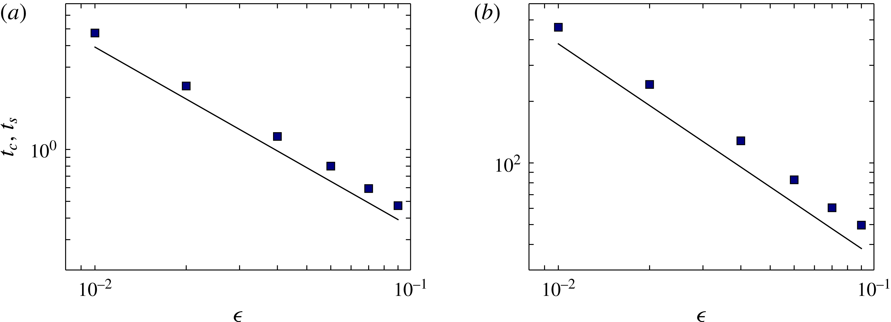
Comparison of analytical singularity times $t_{c}$ , calculated from (5.35), and numerical shock–shock formation times $t_{s}$ , collectively called critical times for (a) strong shocks, $M_{0}=50$ and (b) weak shocks, $M_{0}=1.1$ . $\unicode[STIX]{x1D6FE}=5/3$ for these cases; ——,  $t_{c}$ ; ▪ (navy), $t_{s}$ .

Figure 2 shows the data for the analytical result compared with some points collected from the numerical method, with $\unicode[STIX]{x1D6FE}=5/3$ . The analytical result underestimates the numerical $t_{s}$ at the largest amplitudes by approximately 15 %–26 %. For both cases, the agreement between $t_{c}$ and $t_{s}$ tends to improve slightly as $\unicode[STIX]{x1D716}$ is decreased. These discrepancies are discussed further in § 9.

8.2 Analytical shock shape construction

Although the focus of § 5 is the asymptotic behaviour of the $\unicode[STIX]{x1D706}_{m}$ , and hence the $\hat{z}_{m}(\unicode[STIX]{x1D70F})$ , at high $m$ , the recursion relation (5.22) may be used in the form for $R_{m}(\unicode[STIX]{x1D70F})$ , equation (5.15), and from there in (4.6). 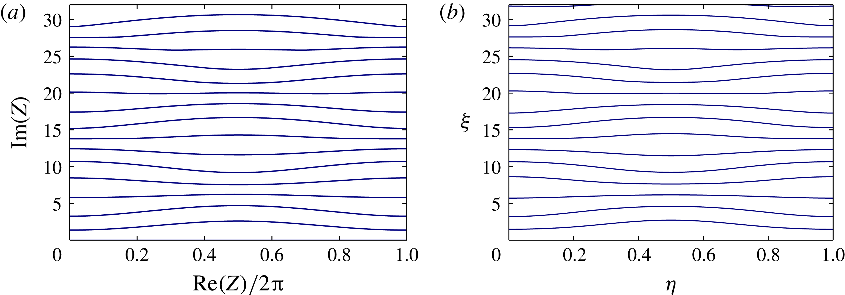Provided the recursion relation is not catastrophically unstable, this generates the leading order of the Fourier coefficients up to some high $m$ , say 512, and may then be used in the Fourier series to reconstruct the physical shock shape, which can in turn be compared with the numerical results from the GSD code. This comparison for $M_{0}=50$ , $\unicode[STIX]{x1D716}=0.08$ is shown in figure 3.

Figure 3.

Comparison of analytical reconstruction of shock shape (a) with numerical GSD results (b) for $M_{0}=50$ , $\unicode[STIX]{x1D716}=0.08$ . The GSD results are contours of the quantity $M_{0}\unicode[STIX]{x1D6FC}$ , which is equivalent to $\unicode[STIX]{x1D70F}$ in the analytical results. Contours are plotted in increments of $\unicode[STIX]{x0394}\unicode[STIX]{x1D70F}=\unicode[STIX]{x1D6E5}(M_{0}\unicode[STIX]{x1D6FC})=2$ . The shock is travelling upwards and amplitudes are artificially amplified twentyfold for visibility. $\text{Im}(Z)$ is equivalent to $\unicode[STIX]{x1D709}$ and is the coordinate parallel to mean shock motion; $\text{Re}(Z)$ is equivalent to $\unicode[STIX]{x1D702}$ and is the coordinate perpendicular to mean shock motion. In (a), the uppermost contour just precedes the singularity formation predicted by (5.35), at $\unicode[STIX]{x1D70F}_{c}=31.614$ .

The shock profiles obtained from the reconstructed analytical result and the GSD numerical solutions are qualitatively quite similar. In fact a further comparison can be drawn in shock oscillation time. At early times, the shock profile should remain smooth and roughly sinusoidal. During this early stage the fundamental frequency of oscillation of the shock can be determined. The analytically predicted time for a single oscillation $t_{osc}$ can be calculated from the fundamental frequency,

(8.5) $$\begin{eqnarray}t_{osc}=\frac{2\unicode[STIX]{x03C0}}{M_{0}a_{0}\text{Im}(\sqrt{1+2b_{1}})},\end{eqnarray}$$

which for the case of $M_{0}=50$ shown in figure 3 is $t_{osc}\simeq 0.205$ . The result found using GSD numerics differs by approximately 2.4 % from the predicted result, and this close agreement in shock oscillation time is visible qualitatively in figure 3. This oscillation time is not a function of perturbation amplitude.

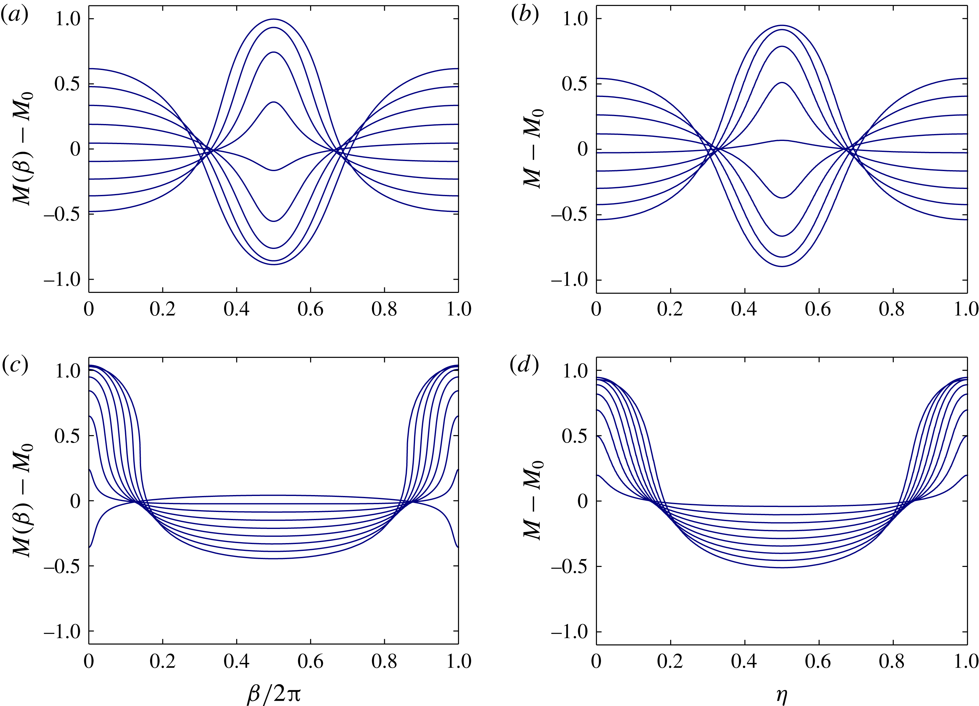
A comparison may also be drawn between the Mach-number profiles during a given time bracket. Figure 4 compares the analytical reconstruction with the numerical result during a time window well before either critical time (figure 4 a,b) and immediately before $\unicode[STIX]{x1D70F}_{c}$ (figure 4 c,d). The results are similar qualitatively in the former case, with opposite-travelling waves on the shock first colliding and then diverging along the shock. Physically, shock–shock formation corresponds to the steepening of these waves into discontinuities as $t\rightarrow t_{s}$ ; for the times just before $\unicode[STIX]{x1D70F}_{c}$ , the analytically constructed profiles are steeper than the GSD result.

Figure 4.

Mach-number profiles on the shock plotted (a,b) over time periods $\unicode[STIX]{x1D70F}=[21,25]$ with increments $\unicode[STIX]{x0394}\unicode[STIX]{x1D70F}=\unicode[STIX]{x1D6E5}(M_{0}\unicode[STIX]{x1D6FC})=0.5$ , and (c,d) $\unicode[STIX]{x1D70F}=[29.614,31.614]$ with increments $\unicode[STIX]{x0394}\unicode[STIX]{x1D70F}=0.25$ . $\unicode[STIX]{x1D70F}$ increasing on the left from top to bottom (a,b); from bottom to top (c,d). The last curve in (c,d) corresponds to $\unicode[STIX]{x1D70F}_{c}=31.614$ . Analytical construction (a,c), calculated by central differences on the reconstructed shock profile; GSD numerical result (b,d), found by nearest-point interpolation on extracted contours of $M_{0}\unicode[STIX]{x1D6FC}$ . The case is $M_{0}=50$ , $\unicode[STIX]{x1D716}=0.08$ . For the numerical result, $M_{0}=\langle M\rangle$ along the profile.

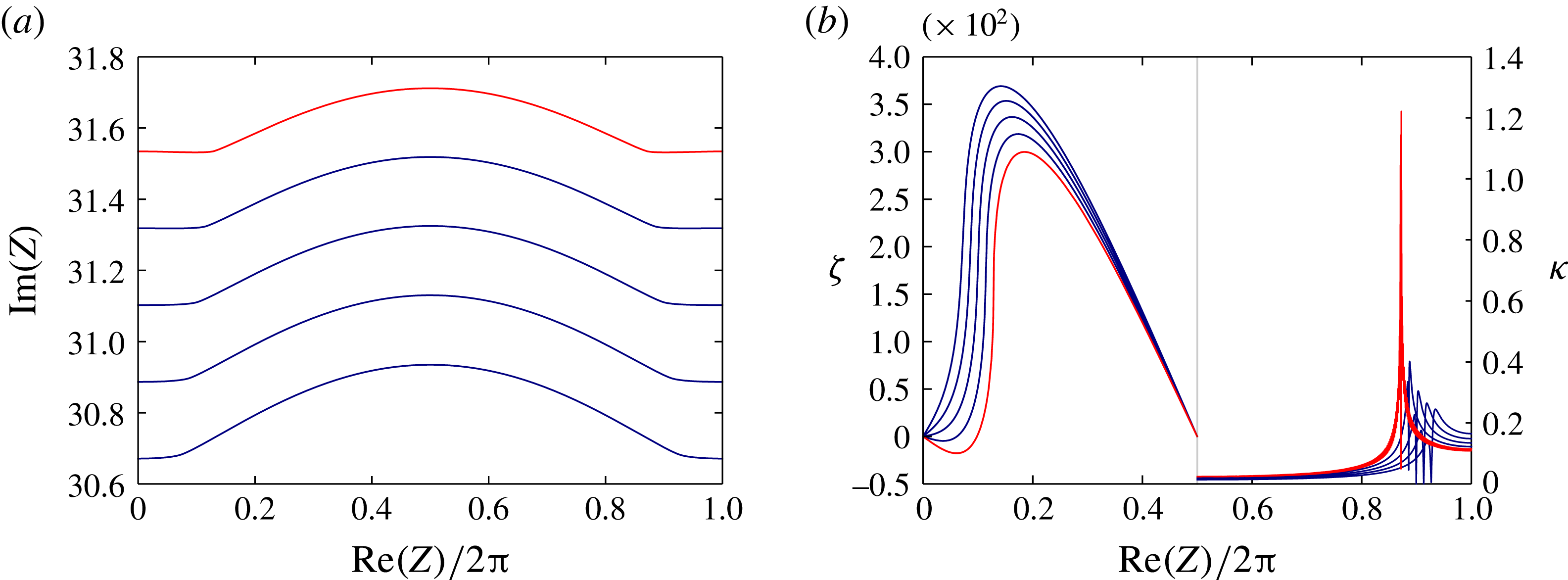
Some insight into the character of the singularity at $t=t_{c}$ can be obtained by examining the shock shape, slope and curvature as $\unicode[STIX]{x1D70F}\rightarrow \unicode[STIX]{x1D70F}_{c}$ . Figure 5 shows the analytically reconstructed shock shape, slope (defined $\unicode[STIX]{x1D70D}=\text{Im}(Z^{\prime })/\text{Re}(Z^{\prime })$ ) and curvature,

(8.6) $$\begin{eqnarray}\unicode[STIX]{x1D705}=\frac{\sqrt{(Z^{\prime }.{Z^{\prime }}^{\ast })(Z^{\prime \prime }.{Z^{\prime \prime }}^{\ast })-[(Z^{\prime }.{Z^{\prime \prime }}^{\ast }+{Z^{\prime }}^{\ast }.Z^{\prime \prime })/2]^{2}}}{(Z^{\prime }.{Z^{\prime }}^{\ast })^{3/2}},\end{eqnarray}$$

primes indicating differentiation with respect to $\unicode[STIX]{x1D6FD}$ . The quantities $Z^{\prime },Z^{\prime \prime }$ were obtained by summing term-by-term differentiation of the Fourier series of $Z$ with 2048 Fourier coefficients. This is valid provided $Z,Z^{\prime }$ remain continuous. Derivatives of higher order than $Z^{\prime \prime }$ do not exist owing to the decay rate $m^{-5/2}$ of the Fourier coefficients.

As $\unicode[STIX]{x1D70F}\rightarrow \unicode[STIX]{x1D70F}_{c}$ , figure 5(a) shows that the shock profile appears to be evolving toward the formation of two kinks, or slope discontinuities. In figure 5(b), the asymmetric (about $\text{Re}(Z)/(2\,\unicode[STIX]{x03C0})=0.5$ ) slope is plotted in $0\leqslant \text{Re}(Z)/(2\,\unicode[STIX]{x03C0})<0.5$ while the symmetric curvature $\unicode[STIX]{x1D705}$ is plotted in $0.5<\text{Re}(Z)/(2\,\unicode[STIX]{x03C0})<1.0$ . The slope is everywhere finite at $\unicode[STIX]{x1D70F}=\unicode[STIX]{x1D70F}_{c}$ but is approaching a discontinuity, while the curvature appears to exist everywhere except possibly at two isolated points where $Z^{\prime \prime }$ may become singular. It can be seen that the maximum shock curvature increases, as $\unicode[STIX]{x1D70F}\rightarrow \unicode[STIX]{x1D70F}_{c}$ , along two converging, oblique lines in the $\text{Re}(Z){-}\text{Im}(Z)$ plane. This effect can also be observed as a prelude to shock–shock formation in figure 2(a) of Mostert et al. (Reference Mostert, Pullin, Samtaney and Wheatley2017).

Figure 5.

(a) Shock-profile perturbation amplified fourfold, (b) split plot of slope $\unicode[STIX]{x1D70D}$ (left half) and curvature $\unicode[STIX]{x1D705}$ (right half). Profiles plotted $\unicode[STIX]{x1D70F}\leqslant \unicode[STIX]{x1D70F}_{c}$ up to $\unicode[STIX]{x1D70F}_{c}=31.6146$ at increments of $\unicode[STIX]{x0394}\unicode[STIX]{x1D70F}=0.2$ , with the profile at $\unicode[STIX]{x1D70F}_{c}$ in red. The line $\text{Re}(Z)/2\unicode[STIX]{x03C0}=0.5$ is a symmetry axis for $\unicode[STIX]{x1D705}$ and an antisymmetry axis for $\unicode[STIX]{x1D70D}$ . $M_{0}=50$ , $\unicode[STIX]{x1D716}=0.08$ , $\unicode[STIX]{x1D6FE}=5/3$ for this case.

8.3 MHD strong-shock dependence on magnetic field strength

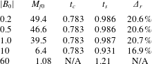
Finally we examine the effect of varying magnetic field on $t_{s}$ for perturbed parallel strong MHD shocks. The code of Mostert et al. (Reference Mostert, Pullin, Samtaney and Wheatley2017) is used with a non-zero magnetic field. The full area–Mach-number ODE is adjusted accordingly and the shock-detection routine remains unchanged. We test the same initial conditions as the gas-dynamic strong-shock case above, $M_{0}=50$ , with a single representative perturbation amplitude $\unicode[STIX]{x1D716}=0.05$ , with uniform magnetic fields $B_{0}=0.2$ , 0.5, 1, 10, 60. This corresponds to unperturbed fast magnetosonic Mach numbers of $M_{f0}=49.4$ , 46.6, 39.5, 6.4, 1.08. The condition that $M_{f}\gg 1$ is marginal in the case $B_{0}=10$ , and clearly not met in the case $B_{0}=60$ ; these are included for comparison. For $B_{0}=60$ particularly it is not clear that (8.3) is the relevant initial condition for the numerical comparison since the analysis of appendix A does not apply.

Table 1.

Comparison of time to shock–shock formation for parallel MHD shocks. $\unicode[STIX]{x1D6E5}_{r}$ is the relative difference of the analytical singularity formation time $t_{c}$ to the numerically determined shock–shock formation time $t_{s}$ . The strong-shock condition is not met in the case $B_{0}=60$ so the analytical result does not apply.

Table 1 compares critical times for the strong-shock MHD case. As expected from the correspondence of the MHD $A{-}M$ relation to the gas-dynamic case, critical times are insensitive to magnetic field strength for sufficiently small values. The relative differences are similar to those observed in the previous gas-dynamic comparisons. The strong-field case, in which $M_{f0}\simeq 1$ , shows a different $t_{s}$ as expected. Note that the case $B_{0}=10$ , with a large but not truly strong $M_{f0}$ , shows some difference to the other cases.