



1. Introduction
The importance of drag reduction (DR) is highlighted by the need to reduce energy consumption and pollutant emission in the next-generation transportation systems. The transportation sector consumes 25 % of the energy budget and produces over 10 % of the global greenhouse gas emissions. These numbers are directly connected to the drag of transportation vehicles. Skin friction is one of the most important sources of drag, contributing up to 55 % of the total drag of commercial aircraft and over 70 % of oil tankers. Various DR techniques have been proposed in the past several decades. See, for example, Karniadakis & Choi (Reference Karniadakis and Choi2003), Kasagi, Suzuki & Fukagata (Reference Kasagi, Suzuki and Fukagata2009), Quadrio (Reference Quadrio2011), Perlin, Dowling & Ceccio (Reference Perlin, Dowling and Ceccio2016) for recent reviews.
Most of the DR strategies target the near-wall coherent structures, including the quasi-streamwise vortices (QSVs) and the velocity streaks, which are closely associated with the skin-friction drag (Orlandi & Jiménez Reference Orlandi and Jiménez1994). The production of Reynolds shear stress is linked directly with the QSVs in the wall layer, which are generally located immediately above and displaced laterally from the high wall shear stress (WSS) region (Bernard, Thomas & Handler Reference Bernard, Thomas and Handler1993; Kravchenko, Choi & Moin Reference Kravchenko, Choi and Moin1993). The well-known events, i.e. ejections, sweeps, bursts and streaky structures, are closely connected to the QSVs (Kim Reference Kim1983; Robinson Reference Robinson1991). The ejection events occur on the up-draught side of the QSVs, leading to the formation of the low-speed streaks (Kline et al. Reference Kline, Reynolds, Schraub and Runstadler1967). On the other hand, the sweep events take place on the down-draught side, resulting in the high-speed streaks and increasing the local WSS. The streaks are unstable to the normal mode instability (Hamilton, Kim & Waleffe Reference Hamilton, Kim and Waleffe1995) and even more so to the non-normal mode instability (Schoppa & Hussain Reference Schoppa and Hussain2002), resulting in the streamwise-dependent disturbance and hence the generation of the new QSVs.
Various passive techniques have been developed for DR in the turbulent boundary layer (TBL), e.g. riblets, compliant surfaces and superhydrophobic materials. Active controls prove to be more effective and robust in DR and has received increasing attention in the literature, such as the wall-normal or in-plane uniform wall oscillation (e.g. Choi, Moin & Kim Reference Choi, Moin and Kim1993; Baron & Quadrio Reference Baron and Quadrio1996; Carlson & Lumley Reference Carlson and Lumley1996), the spanwise or streamwise-travelling wave-like wall-normal deformation (e.g. Tomiyama & Fukagata Reference Tomiyama and Fukagata2013; Li et al. Reference Li, Roggenkamp, Hecken, Jessen, Klaas and Schröder2018) and externally introduced large-scale streamwise vortices (Schoppa & Hussain Reference Schoppa and Hussain1998). Among the active techniques, blowing and suction, the subject of this paper, are potentially implementable in engineering applications and have been rather extensively studied. It is now well established that uniform blowing reduces local WSS but increases the turbulence intensity, while suction does the opposite (e.g. Park & Choi Reference Park and Choi1999; Kametani & Fukagata Reference Kametani and Fukagata2011). Global uniform blowing on the wall over the entire TBL may produce a DR of 70 %–75 % (e.g. Kametani & Fukagata Reference Kametani and Fukagata2011; Kornilov & Boiko Reference Kornilov and Boiko2012). Localized uniform blowing through a spanwise slit in the TBL has also been investigated both experimentally and numerically (e.g. Park & Choi Reference Park and Choi1999; Krogstad & Kourakine Reference Krogstad and Kourakine2000; Kim, Kim & Sung Reference Kim, Kim and Sung2003). Locally, DR may reach up to 70 %, though often accompanied by a drag increase further downstream. Park & Choi (Reference Park and Choi1999) suggested that the QSVs are lifted away from the wall by the localized blowing, so that the interaction between the QSVs and the wall is weakened, resulting in lessened friction. At the same time, the lifted QSVs become stronger, contributing to an increase of the turbulence intensity and WSS further downstream of the slot.
Attempts have also been made for unsteady blowing control. Tardu (Reference Tardu2001) experimentally studied the effect of periodically varying blowing through a spanwise slot in the TBL, achieving a local maximum DR of 45 % at 20 wall units downstream of the slot. However, there was a drag increase by 200 % over 80–300 wall units downstream of the slot. Tardu & Doche (Reference Tardu and Doche2009) deployed a periodical but dissymmetric blowing, characterized by a rapid acceleration phase in the blowing velocity followed by a slow deceleration, rather than the sinusoidal waveform used by Tardu (Reference Tardu2001). A local maximum DR of 53 % was observed and the DR effect persisted to 1000 wall units downstream. The improvement was ascribed to much weaker spanwise vortical structures generated by the dissymmetric blowing than by the sinusoidal waveform. The blowing velocity in Tardu (Reference Tardu2001) and Tardu & Doche (Reference Tardu and Doche2009) is large, approximately 30 % of the free-stream velocity, as their focus was on the newly generated spanwise vortical structure rather than modifying near-wall coherent structures in the natural TBL (Kim & Sung Reference Kim and Sung2006). Using a relatively small periodical blowing amplitude, less than 5 % of the free-stream velocity, through a spanwise slot, Kim & Sung (Reference Kim and Sung2003, Reference Kim and Sung2006) achieved numerically a local maximum DR of 75 % in the TBL. Such a pronounced DR with a much smaller blowing velocity is likely to be linked to a larger streamwise extent (100 wall units) of their slot, to be compared with only 8 wall units in Tardu's (Reference Tardu2001) and Tardu & Doche's (Reference Tardu and Doche2009) experiments.
Attention has also been given to wall-normal blowing through streamwise slits. Rathnasingham & Breuer (Reference Rathnasingham and Breuer2003) used one spanwise array of synthetic jets through streamwise slits to manipulate a TBL, and achieved a local maximum DR of only 7 %. Abbassi et al. (Reference Abbassi, Baars, Hutchins and Marusic2017) deployed one array of nine wall-normal blowing jets through streamwise slits in a TBL with a friction Reynolds number as high as 14 400. With an aim to manipulate the coherent structures in the outer region, they used a very large blowing amplitude, 64 % of the free-stream velocity, and obtained a local maximum DR of 3.2 %, although the DR persisted for more than five times the boundary layer thickness. Nevertheless, our knowledge on the technique based on one array of unsteady blowing jets through streamwise slits is rather limited. For example, could this technique produce a substantial DR accompanied by net power saving? If so, what are the underlying mechanisms? The control performance depends on a number of parameters such as the blowing frequency and amplitude, and the overall spanwise and streamwise extents of the jet array. This dependence has yet to be documented in detail. Furthermore, could we find a scaling parameter that dictates DR?
This work aims to address the issues raised above. Its initiation is also inspired by Bai et al.'s (Reference Bai, Zhou, Zhang, Xu, Wang and Antonia2014) investigation, who deployed one spanwise array of longitudinally arranged oscillating piezo-ceramic actuators to produce a spanwise-travelling wave of wall-normal deformation in the TBL. They achieved a local maximum DR of 50 %. However, the drag recovered rapidly, probably because of a short effective oscillating length due to the cantilever-supported actuators. One naturally wonders whether the DR would persist if the effective length were substantially increased. In this work, we deploy one array of unsteady blowing jets through a large number of narrow streamwise slits, and the actuation length greatly exceeds that in Bai et al. (Reference Bai, Zhou, Zhang, Xu, Wang and Antonia2014). The dependence of DR on the control parameters, including the blowing amplitude and frequency, is investigated in detail. Extensive measurements are conducted to capture the flow structure with and without control using hot-wire, particle image velocimetry (PIV) and smoke-wire flow visualization techniques. Experimental details are given in § 2. Results are presented and discussed in §§ 3–6. This work is concluded in § 7.
2. Experimental details
2.1. Generation of TBL
Experiments were conducted in a closed-circuit wind tunnel with a 5.6 m long horizontal test section of 0.8 m in width and 1.0 m in height at Harbin Institute of Technology (Shenzhen). A 4.8 m long flat plate with 0.78 m in width and 0.015 m in thickness, rounded at the leading edge, was placed vertically in the test section, slightly inclined with respect to flow to produce a zero-pressure-gradient boundary layer. The flow passage between the flat plate surface and the wind tunnel wall was 0.6 m. Flow separation from the leading edge was minimized by tuning the pitch angle of a 0.2 m long tail-end board. The flow was tripped at 0.1 m downstream of the leading edge by two spanwise arrays of screws separated longitudinally by 15 mm and stagger mounted, as in Bai et al. (Reference Bai, Zhou, Zhang, Xu, Wang and Antonia2014). Each screw, 15 mm in height, was separated from its adjacent ones by 15 mm in the spanwise direction. Measurements were conducted at a free-stream velocity U∞ = 2.4 m s−1 and the corresponding free-stream longitudinal turbulence level was 0.4 %. The characteristic parameters of the uncontrolled TBL at the test position, 3.2 m downstream of the leading edge of the plate (figure 1), are given in table 1, where δ is the boundary layer thickness based on the location of 99 %U∞, θ is the momentum thickness, H 12 is the shape factor, Reθ is the θ-based Reynolds number, uτ is the friction velocity, lv (≡ ν/uτ, ν is the kinematic viscosity) and tv  $({\equiv} \nu /u_\tau ^2)$ are the viscous length and time scales, respectively.
Schematic of the experimental set-up, including actuator, its installation and measurements (not to scale; units in mm).

Characteristic parameters of the uncontrolled TBL.

2.2. Jet generation
One array of nine streamwise slits is placed 3.2 m downstream from the leading edge (figure 1). This number is increased to 31 when the smoke-wire flow visualization is carried out in order to improve the quality of flow images. The increase of slit number may reduce the three-dimensional effect of meandering streaks, i.e. the interaction between the uncontrolled and controlled flows when developing downstream. This may lead to an appreciably postponed drag recovery but essentially no effect on the DR near the actuator. Each slit is 20 mm in length, 0.5 mm in width and 3 mm in depth. The centre-to-centre spacing between two adjacent slits is 2 mm. Air from a compressor passes a filter, a pressure relief valve, a throttle valve, a flow meter and an electromagnetic valve, a plate of 30 mm × 120 mm with eight equally separated holes of 10 mm in diameter, and a contraction with an area ratio of 6, which acts to ensure the uniformity of jets through the slits. The electromagnetic valve works on a 20 % duty cycle with a frequency range of f = 5–400 Hz, which is controlled by a real-time signal-processing platform dSpace. The flow rate is manually adjusted by a simple throttle. The instantaneous jet exit velocity Uout ,c at the centre of each slit is confirmed to be longitudinally rather uniform and unchanged from one slit to the other. The jet exit velocity  ${A^ + } = \overline {{U_{out,c}}} /{u_\tau }$ is in the range of 0–2 and
 ${f^ + } = f\nu /u_\tau ^2$ is 0.007–0.56. In this paper, the overbar denotes a time-averaged quantity; unless otherwise stated, the superscript ‘+’ and ‘*’ represent normalization by the inner and outer scales of the uncontrolled TBL, respectively. The coordinates x, y and z are along the streamwise, wall-normal and spanwise directions, respectively, and their origin is defined at the mid-point of the slit array trailing edge, as shown in figure 1; U
 $({\equiv} \bar{U} + u)$, V
 $({\equiv} \bar{V} + v)$ and W
 $({\equiv} \bar{W} + w)$ are the instantaneous velocities along the x, y and z directions, respectively, where u, v and w are their corresponding fluctuating components.
2.3. Flow measurements
The WSS is measured, following for example Hutchins & Choi (Reference Hutchins and Choi2002), from the slope of the mean streamwise velocity profile in the viscous sublayer. A single tungsten wire of 5 μm diameter, operated on a constant temperature circuit (Dantec Streamline Pro) at an overheat ratio of 1.8, is used to measure the streamwise velocity. The signals from the hot-wire are filtered at a cutoff frequency of 3 kHz and then digitized using a 16-bit analogue/digital board at a sampling frequency of 6 kHz. The duration for each record of the hot-wire signal is 40 s so that the mean and root mean square (r.m.s.) values of the velocity are converged to within 0.0014 and 0.0027 m s−1, corresponding to 0.06 % and 0.11 % of the free-stream velocity, respectively. This hot-wire probe is mounted on a computer-controlled three-dimensional traversing mechanism, whose spatial resolution is 3.125 μm along each spatial direction.
A LaVision time-resolved PIV system is used to measure the TBL in different planes with and without control under the control conditions, i.e. A+ = 1.42 and f+ = 0.42, where the maximum local DR is achieved. The flow is seeded with peanut oil droplets, with an average diameter of 1 μm, generated by a TSI 9307-6 particle generator. The laser source has a maximum energy output of 30 mJ per pulse. Particle images are captured using one CCD camera operated on the mode of the double frames (2016 pixels × 2016 pixels), with an interval of 120 μs between the frames. The image magnification factors are 0.03, 0.04 and 0.03 mm per pixel in the y–z, x–z and x–y planes, respectively. A total of 3000 image pairs were captured in each plane at a sample frequency of 800 Hz. A convergence test for the PIV-measured mean velocity in the TBL confirmed that the distributions of streamwise velocities obtained from the image pairs of 3000, 4000 and 5000 all collapse very well with a maximum departure of approximately 1 %.
The smoke-wire flow visualization is conducted in the x–z plane of y = 1 mm, corresponding to 6 wall units for the uncontrolled TBL, with and without control. A nickel–chromium wire of 0.05 mm diameter, strained and supported at both ends, is placed 3 mm upstream of the leading edge of the slit jet array, perpendicularly to mean flow in the plane of y = 0.9 mm (5 wall units for the uncontrolled TBL) parallel to the flat plate. The wire is coated with paraffin oil for the entire length. A uniform smoke sheet may be produced once the wire is heated by a direct electric current with a maximum of 30 mA. The same LaVision PIV system is deployed to capture flow images. The flow is illuminated by a laser sheet of 1.0 mm thick. The flow images are recorded at 800 frames per second. U∞ is set at 1.8 m s−1 (Reθ = 1050) to ensure reasonably high-quality flow visualization images.
In the estimate of input fluid energy into the TBL, discussed in § 6.6, the pressure loss of the injected fluid through the array of slits from the contraction to the TBL is excluded. To measure this loss, pressure taps of 1 mm diameter are drilled 5 mm downstream of the actuator trailing edge and also on the contraction chamber, as shown in figure 1. Pressure at these points is measured using microphones (GRAS 46BL). Each microphone is fitted with a sponge rubber wind screen in order to suppress noise from other sources. The background noise generated by the wind tunnel fan is also measured simultaneously and then subtracted from the obtained pressure signals. The signals are captured simultaneously using a NI USB-6341 A/D board, built with on-board software-controlled anti-aliasing filters. The signals are digitized at a sampling frequency of 250 Hz. The sampling duration is 40 s.
3. Actuator-generated flow
It is important to document first the flow generated by the blowing slit jets in the absence of the TBL. A single hot-wire is placed parallel to and above the slits to measure Uout ,c at the slit exit when U ∞ = 0. At A+ = 1.42, figure 2 illustrates the time histories of jet exit velocity  $U_{out,c}^ + $ measured at the streamwise and spanwise centre of the middle slit using a hot-wire and the input signal E*, whose 0 and 1 correspond to the off- and on-state of the magnetic valve, respectively. Note that there is a time delay of 4.8 ms from the instant when the magnetic valve is switched on to the sudden rise of
 $U_{out,c}^ + $. The ideal performance of unsteady blowing is that the jet exit velocity and frequency are independent of each other; for example, the velocity or its maximum remains unchanged when the excitation frequency varies. However, this is extremely difficult, if not impossible, experimentally due to the limitation of the present state-of-the-art technology (magnetic valves) and the inertia of the air in the tube. The performance can be improved if the length (0.5 m) of the tube from the electromagnetic valve to the slit nozzle exit could be reduced. A change in the magnetic-valve-controlled frequency will unavoidably cause the jet exit velocity to vary, as shown in the characteristic curve between
 $U_{out,cmax}^ + $ and f+ (figure 3a). Given f+ ≤ 0.14, the
 $U_{out,c}^ + $ signal varies between its maximum and zero, as illustrated in figure 2(a,b); however, for f+ > 0.14, this velocity could not go to zero, albeit exhibiting the specified periodic variation (figure 2c,d) as is evident in the spectra (figure 3b). The time-averaged jet exit velocities
 $\overline {U_{out,c}^ + } $ (figure 3c) measured at the centrelines of the nine slits are almost identical, with a maximum deviation of 0.9 %. The deviation is less than the uncertainty of the hot-wire measurement (0.0014 m s−1 or 1.02 % of
 $\overline {U_{out,c}^ + } $), indicating a good uniformity of the blowing jets.
Time histories of the inner-scale-normalized velocity  $U_{out,c}^ + $ at jet exit (black curve) measured using a hot-wire placed at (x+, y+, z+) = (66.7, 6.7, 0) and the input signal E* (red curve) of the magnetic valve. The magnetic valve switches off and on once E* reaches 0 and 1, respectively. Control parameter: Q = 2.625 l min−1 and A+ = 1.42; (a) f+ = 0.028, (b) f+ = 0.14, (c) f+ = 0.42, (d) f+ = 0.56.

(a) Dependence on f+ of the maximum instantaneous jet exit velocity  $U_{out,cmax}^ + $. Q = 2.625 l min−1 and A+ = 1.42. (b) Power spectral density function
 $E_u^ +$ of the exit velocity Uout ,c of slits at (A+, f+) = (1.42, 0.42). (c) Distribution of the time-averaged jet exit velocity
 $\overline {U_{out,c}^ + } $ measured by the hot-wire at (x+, y+) = (−66.7, 6.7). Control parameters: f + = 0.42, A+ = 1.42.

In the presence of the TBL, the present periodic blowing jets through slits produce two effects. The first is to add zero-streamwise-momentum fluid into the TBL, as noted in previous investigations (e.g. Park & Choi Reference Park and Choi1999; Kametani & Fukagata Reference Kametani and Fukagata2011). The injection of the low-momentum fluid shifts the mean velocity profile away from the wall and decreases the streamwise velocity near the wall, resulting in DR (Kametani & Fukagata Reference Kametani and Fukagata2011). The second is to generate one array of counter-rotating streamwise vortices near the wall. This is evident from the iso-contours of the instantaneous streamwise vorticity  $\omega _x^ +$ (= ∂W+/∂y+ − ∂V+/∂z+) and the velocity vectors (V+, W+) in the PIV-measured y–z plane at x+ = −67 (figure 4), which display one array of periodically varying and highly regularized streamwise vortices, with a pair of counter-rotating vortices associated with each blowing jet. Note that the instantaneous streamwise vorticity structures are not perfectly symmetric, which is perhaps not unexpected. The streamwise vorticity structures shown in figure 4 result from the interaction between the blowing jets and the near-wall turbulence. The latter is spanwise non-uniform. The nine slits cover an area of about 120 wall units in the spanwise direction, larger than the mean separation (100 wall units) between the low-speed streaks (e.g. Kline et al. Reference Kline, Reynolds, Schraub and Runstadler1967; Robinson Reference Robinson1991). As such, there are in general at least one low-speed and one high-speed streak over the span of the slit array, accounting for the non-uniform distribution of the instantaneous streamwise vorticity along spanwise direction. This result resembles the streamwise vortex array generated by the wall-normal oscillation of the piezo-ceramic actuators in Bai et al. (Reference Bai, Zhou, Zhang, Xu, Wang and Antonia2014). However, there are differences. First of all, the latter vortices are co-rotating. Further, the streamwise extent of the present vortex array is obviously much longer than that in Bai et al. (Reference Bai, Zhou, Zhang, Xu, Wang and Antonia2014), due to the larger effective length of the actuator. Apparently, the present actuation is distinctly different from previously reported TBL control based on steady or pulsed spanwise blowing (Tardu Reference Tardu2001; Tardu & Doche Reference Tardu and Doche2009) or uniform blowing (e.g. Kametani & Fukagata Reference Kametani and Fukagata2011) where no streamwise vortices are observed.
Instantaneous streamwise vorticity  $\omega _x^ +$ (= ∂W+/∂y+ − ∂V+/∂z+) and cross-stream velocity vectors (V+, W+) measured by PIV in the y–z plane x+ = −67. Periodic blowing jets with control parameters (A+ = 1.42, f+ = 0.028).

4. Control performance
4.1. Dependence of DR on control parameters
The time-averaged local WSS  $\overline {{\tau _w}} $ is estimated from the mean streamwise velocity gradient in the viscous sublayer. Figure 5 presents the distribution of the time-averaged streamwise velocity near the wall along the y direction. The hot-wire measurement below y+ < 3 is apparently influenced by the wall effect. As such, only the data points that fall within 3 < y+ < 5, i.e. a total of 7 points, are used to determine the slope of the streamwise velocity. Following Hutchins & Choi (Reference Hutchins and Choi2002), the uncertainty of the measured WSS from linear fitting is estimated to be less than 1.8 % at U∞ = 2.4 m s−1. A comprehensive study of the dependence of local DR on A + and f + is conducted at x+ = 33 (z+ = 0), where the hot-wire measurement is already cleared of the direct blowing jet effect. The local drag change is defined as
 ${\delta _{{\tau _w}}} = [{(\overline {{\tau _w}} )_{on}} - {(\overline {{\tau _w}} )_{off}}]/{(\overline {{\tau _w}} )_{off}}$, where the subscripts ‘on’ and ‘off’ denote the values with and without control, respectively. The standard uncertainty
 ${s_R}$ of
 ${\delta _{{\tau _w}}}$ can be calculated through
 ${s_R} = (1 + {\delta _{{\tau _w}}})\sqrt {s_{off}^2 + s_{on}^2}$, where soff and son are the uncertainties of the hot-wire-measured WSS without and with control, respectively (Yao, Chen & Hussain Reference Yao, Chen and Hussain2018). The total uncertainty of
 ${\delta _{{\tau _w}}}$ is defined as
 $1.96{s_R}$, corresponding to the standardized 95 % confidence interval.
Distribution of mean streamwise velocity in the near-wall region along y direction normalized by (a) inner scale and (b) outer scale.

At the low control frequency range, f+ = 0.007–0.14, the local friction change depends on both A+ and f+ (figure 6a), and  ${\delta _{{\tau _w}}}$ displays an obvious local minimum (i.e. maximum friction reduction) for each f+ at the optimum A+, i.e.
 $A_{opt}^ + $. For example,
 $A_{opt}^ + $ is 0.57, 0.86, 1.14 and 1.71 for f+ = 0.007, 0.021, 0.028 and 0.14, respectively. The DR decreases once A+ exceeds
 $A_{opt}^ + $. Two factors may account for the observation. Firstly, the penetration depth of the actuation is crucially important; the best control effect occurs when the height of the blowing-induced vortices is comparable to the thickness of the viscous sublayer. As a matter of fact, the present result is similar to Bai et al.'s (Reference Bai, Zhou, Zhang, Xu, Wang and Antonia2014) observation that the DR was more pronounced with the increasing oscillation amplitude of the actuators, but contracted after reaching its maximum at
 $A_{opt}^ +\approx 2$, where the penetration depth of the actuation was comparable to the viscous-sublayer thickness. The similarity may not be surprising. Although actuators are different between the two studies, the streamwise vortex array generated near the wall in both cases acts as a barrier to alleviate the interaction between the coherent motions such as the sweep events, and the wall, thus causing a DR. Secondly, the strength of the blowing-induced vortices also plays a role. An over-strengthened streamwise vortex array once
 ${A^ + } > A_{opt}^ + $ may lead to an increase in the coherent shear stress and adversely affect the DR. It is well established that the net effect of the upwash and downwash effects on each side of the streamwise vortices is to increase the WSS in a TBL (e.g. Kravchenko et al. Reference Kravchenko, Choi and Moin1993). After reaching its optimum strength to manipulate the TBL, any further increase in the strength of the streamwise vortex array would not keep improving the control effect, but lead to a rapid growth of the additional WSS. In spite of distinct DR mechanisms, Yao et al. (Reference Yao, Chen and Hussain2018) introduced using direct numerical simulation (DNS) a spanwise body force and generated large-scale streamwise vortices (LSSVs) in a channel flow. The LSSVs acted to stabilize the streaky structures, resulting in a maximum spatially averaged DR of 19 %. They also observed that the DR became less pronounced as the coherent shear stress grew for over-strengthened LSSVs. They proposed, based on the Fukagata–Iwamoto–Kasagi (FIK) identity (Fukagata, Iwamoto & Kasagi Reference Fukagata, Iwamoto and Kasagi2002), that the coherent shear stress increased rapidly with the strengthened LSSVs, which accounted for the decreased DR.


At the high frequency range, i.e. f+ = 0.28–0.56, the measured local DR becomes different, since  ${\delta _{{\tau _w}}}$ exhibits little dependence on f+. The
 ${\delta _{{\tau _w}}}$ values collapse for given A+ and keeps declining for increasing A+. Furthermore,
 ${\delta _{{\tau _w}}}$ is always smaller at high f+ (≥0.28) than at low f+ given the same A+. Two factors may contribute to the observations. Firstly, the collapse of the
 ${\delta _{{\tau _w}}}$ profiles is connected to the fact that the difference in the Uout ,cmax becomes negligibly small and changes little at large f+ (figure 3a), implying a small and almost constant penetration depth. As shown in figure 4, the jet-induced streamwise vortices at f+ = 0.028 appear producing a perturbation to the flow up to y+ = 15 in the buffer layer. Bai et al. (Reference Bai, Zhou, Zhang, Xu, Wang and Antonia2014) assumed that, being positively related to the induced wall-normal velocity, the oscillating amplitude of the piezo-ceramic actuators could be linearly related to the penetration depth. In the present study, Uout ,max at f+ = 0.028 is approximately three times that at f+ = 0.42 (figure 2). It may be inferred that the perturbation to flow at f+ = 0.42 is comparable to the thickness of the viscous sublayer (y+ < 5) following Bai et al.'s (Reference Bai, Zhou, Zhang, Xu, Wang and Antonia2014) assumption. This inference is consistent with previous reports that the penetration depth must remain small to avoid the disruption of the outer flow for the purpose of effective control. In their DNS study, Du, Symeonidis & Karniadakis (Reference Du, Symeonidis and Karniadakis2002) deployed a transverse travelling wave and produced the maximum DR of 30 % in a turbulent channel flow when the penetration depth was comparable to the viscous sublayer. Quadrio & Ricco (Reference Quadrio and Ricco2011) reported that the maximum DR took place when the thickness of the generalized Stokes layer was 6.5 wall units for the streamwise-travelling wave control. The interaction between the Stokes layer and the turbulent flow would be less effective beyond an optimal thickness of the Stokes layer (Quadrio, Ricco & Viotti Reference Quadrio, Ricco and Viotti2009). As such, given the same A+, the smaller penetration depth, which is comparable to the thickness of the sublayer, may account for the more pronounced DR at high f+. Secondly, an increased A+ is accompanied by a larger mass flow rate of the zero-streamwise-momentum fluid, which acts to decrease the near-wall streamwise velocity, causing a further drop in
 ${\delta _{{\tau _w}}}$. However, a larger mass flow rate implies an increased energy input, which may have an adverse effect on the control efficiency. Figure 6(b) presents the dependence of
 ${\delta _{{\tau _w}}}$ on the inner-scale-normalized maximum jet exit velocity
 $U_{out,cmax}^ + $. The knowledge obtained from this figure is similar to that of
 ${\delta _{{\tau _w}}}$ on A+ (figure 6a).
Unless otherwise stated, the following discussion is presented for the case of  ${\delta _{{\tau _w}}} \approx{-} 70\,\%$ under A + = 1.42 and f + = 0.42, which is a compromise of substantial DR and good control efficiency. It is worth pointing out that no flow separation takes place at these control parameters. The shape factor H is 1.41 without control and increases to a maximum value of 1.47 when control is applied, which is much smaller than the critical value of 2 for flow separation (Simpson, Strickland & Barr Reference Simpson, Strickland and Barr1977). Tardu (Reference Tardu2001) deployed unsteady wall-normal blowing through a spanwise slot in the TBL (Reτ ≈ 473), and no flow separation was observed given A+ = 8. The present A+ is less than 2 (Reτ = 572), which provides another support for the absence of flow separation.
4.2. Downstream recovery of local WSS
The WSS recovers gradually downstream and reaches the natural state at x+ ≈ 500 (figure 7). A small overshoot or drag increase up to 7 % occurs further downstream, which drops gradually to zero by x + ≈ 1500. Using an array of piezo-ceramic actuators with the same streamwise length as the present slits, Bai et al. (Reference Bai, Zhou, Zhang, Xu, Wang and Antonia2014) obtained a local DR of approximately 50 % at x+ = 17, which fully recovered at x+ = 160. Two reasons may account for the present better performance in terms of DR and its associated length than Bai et al. (Reference Bai, Zhou, Zhang, Xu, Wang and Antonia2014). Firstly, although with the same length, the cantilever-supported piezo-ceramic actuator has a significantly shorter effective length than the other. Secondly, the injection of zero-streamwise-momentum fluid into the TBL contributes to the DR (e.g. Kametani & Fukagata Reference Kametani and Fukagata2011; Kornilov & Boiko Reference Kornilov and Boiko2012; Stroh et al. Reference Stroh, Hasegawa, Schlatter and Frohnapfel2016). The present overshooting further downstream is not surprising, which is an inherent attribute of local blowing techniques. For example, the overshoot was numerically observed by Park & Choi (Reference Park and Choi1999) and Kim & Sung (Reference Kim and Sung2006), who used steady and unsteady wall-normal blowing through a spanwise slot, respectively, and also experimentally by Tardu (Reference Tardu2001) who deployed spanwise slot blowing. Park & Choi (Reference Park and Choi1999) suggested that the QSVs lifted by blowing grew stronger downstream, resulting in an increase in the turbulence intensity and also the WSS. Nevertheless, Stroh et al. (Reference Stroh, Hasegawa, Schlatter and Frohnapfel2016) observed no overshoot in their DNS study of local blowing in a TBL. They advocated that the drag increase would occur given the blowing region was longitudinally small but not if this region was large.
Variation of  ${\delta _{{\tau _w}}}$ with the distance downstream of the actuator at z + = 0. Control parameters: A + = 1.42, f+ = 0.42.

5. Alterations to the flow structure
5.1. Statistics of streamwise velocity
Figures 8(a) and (b) presents the mean streamwise velocity profiles normalized by the actual inner and outer scales, respectively, measured at x+ = 33 and z+ = 0. Note that the rightmost plot is equivalent to using unmanipulated wall units, since external units are unaffected by control. In the absence of control, the  $\overline {{U^ + }} $ profile agrees well with Bai et al. (Reference Bai, Zhou, Zhang, Xu, Wang and Antonia2014) and follows the law of wall, showing a linear near-wall region for y+ < 5 and a logarithmic region for 30 < y+ < 170 (figure 8a) characterized by a von Kàrmàn constant of 0.41 and an intercept of 5.1. These observations suggest that the uncontrolled TBL is fully developed at the measurement location. Under control, both linear and log regions are still evident. Owing to the chosen scaling, the two linear regions in figure 8(a) are superimposed, whereas with the alternative outer scaling of figure 8(b) the reduced streamwise momentum near the wall is clearly visualized. The logarithmic region is shifted upwards compared with the uncontrolled TBL: this is a well-known feature of flows with DR, which presents a thickened viscous sublayer. Together with the vertical shift, a minor increase in the slope of the log layer is also observed, pointing to a smaller value of the von Kàrmàn constant. Gatti & Quadrio (Reference Gatti and Quadrio2016) proved for parallel flows that DR by active spanwise control can be described as a special sort of roughness which reduces friction, and that the upward shift is equivalent to DR once the Reynolds number (Re) is known. Skote (Reference Skote2014) reports similar data for the flat-plate TBL; by extrapolating at the observed, large value of DR, very similar values of shift and slope change are observed. This serves as a further indirect confirmation of the reliability of the friction measurements. Moreover, these changes are supposed to be Re independent (Skote Reference Skote2014; Gatti & Quadrio Reference Gatti and Quadrio2016), hence they represent a more robust information than simply the numerical value of DR, which necessarily depends on Re.
Wall-normal distribution of the streamwise mean velocity (panels a, c) and the root-mean-square value of its fluctuations (b, d) measured at (x+, z+) = (33, 0). Quantities are normalized by the actual inner (a, b) and outer (c, d) scales. Control parameters: A + = 1.42, f + = 0.42.

The wall-normal extent of the altered flow is readily discernible from the outer-scale-normalized mean velocity profile (figure 8b). Although the jet-induced streamwise vortices are largely confined within the viscous sublayer,  $\bar{U}/{U_\infty }$ under control shows an appreciable departure from the uncontrolled flow up to at least y = 0.065δ or y + = 37, due to both the injection of zero-streamwise-momentum fluid and the existence of the jet-induced vortices. For y/δ > 0.065, the
 $\bar{U}/{U_\infty }$ profile remains almost unchanged.
The r.m.s. value  $u_{rms}^ +$ of the fluctuating streamwise velocity component u, normalized by both inner and outer scales (figure 8c,d) in the absence of control, agrees well with Bai et al. (Reference Bai, Zhou, Zhang, Xu, Wang and Antonia2014), providing another indirect validation for the present measurements. Under control,
 $u_{rms}^ +$ rises rapidly and exceeds the uncontrolled value until y+ ≈ 355. The maximum
 $u_{rms}^ +$ increases from 2.74 without control to 5.65 with control. Note that
 $u_{rms}^ +$ under control becomes smaller than the uncontrolled at y+ > 220, resulting from normalization by the local wall variables, not from the control. The umrs/U∞ profile (figure 8d) may give a more intuitive view of the control-affected area. Under control, umrs/U∞ becomes much smaller than the uncontrolled flow for y/δ < 0.02 or y+ < 11, indicating weakened turbulence intensities near the wall, which is beneficial for the DR. This is opposite to the distribution of
 $u_{rms}^ +$ which is larger than the uncontrolled flow in this region. The difference is ascribed to the greatly changed local inner scales under control due to large local DR. For example, uτ decreases from 0.105 to 0.058 m s−1 while
 $l_v$ increases from 0.15 to 0.27 mm. At 0.02 < y/δ < 0.13 (11 < y+ < 74), umrs/U∞ exceeds its uncontrolled counterpart due to the strengthened QSVs. The location of the maximum umrs/U∞ moves from y/δ = 0.021 to y/δ = 0.033, i.e. from y+ = 11.5 to y+ = 18.5. As u rms is closely associated with the QSVs (Wallace Reference Wallace2016), the shift in its maximum indicates that the QSVs are lifted due to the existence of the jet-induced streamwise vortices near the wall and the injection of zero-streamwise-momentum fluid, which is in conformity to the observed DR. Park & Choi (Reference Park and Choi1999) suggested that the lifted QSVs grew downstream in strength, resulting in an increase in turbulence intensity. The umrs/U∞ profiles collapse with and without control for y/δ > 0.13, or y+ > 74, where the fluid structures can hardly be affected by periodic blowing because of the present small A+.
5.2. Streaky structures
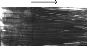
The flow structure obtained from flow visualizations is examined qualitatively in order to gain some insight into the flow physics behind the observed DR. Note that the incoming velocity is reduced to 1.8 m s−1 in order to capture high quality flow visualization images. Figures 9(a) and 9(b) presents the typical images of instantaneous near-wall flow structures from the smoke-wire flow visualization in the x–z plane without and with control, respectively. The laser sheet is fixed at y + = 6, while the smoke-wire is placed at y + = 5 (cfr. § 2). In the absence of control, high- and low-speed streaks are lying side by side as indicated in figure 9(a). The average spanwise spacing between low-speed streaks is approximately 100 wall units, in agreement with a large number of works, starting with the pioneering Kline et al. (Reference Kline, Reynolds, Schraub and Runstadler1967) hydrogen bubble visualization. Video clips (see supplementary movies, https://doi.org/10.1017/jfm.2021.439) indicate that smoke filaments from the smoke-wire are entangled and raised to form thick longitudinal smoke tubes. These tubes tend to slow down, forming low-speed streaks, and are captured by the laser sheet, resulting in white-coloured streaks. On the other hand, dark colour corresponds to the high-momentum fluid moving towards the wall. Once control is applied, the flow structures are greatly modified. The large low- and high-speed streaks are no longer visible over the slit array all the way down to x+ ≈ 160. Instead, we see smaller-scale longitudinal structures, which are more stable and less meandering than the uncontrolled flow. The flow thus exhibits a signature of local relaminarization, resembling Bai et al.'s (Reference Bai, Zhou, Zhang, Xu, Wang and Antonia2014) observation. This is fully consistent with the reduced umrs/U∞ at y + = 6 (figure 8d). The instability of the streaks is essential for the generation of new QSVs in the TBL (Schoppa & Hussain Reference Schoppa and Hussain2002; Kim Reference Kim2011). The stabilized streaks partially inhibit the near-wall turbulence regeneration cycle and therefore account for the reduced WSS. Note that the width and the spanwise spacing between the small structures under control is much smaller than their counterpart in Bai et al. (Reference Bai, Zhou, Zhang, Xu, Wang and Antonia2014). This is attributed to the much longer effective length of present blowing actuation, which is also responsible for the more pronounced local DR and the longer drag recovery distance. At x+ > 160, the larger streaky structures begin to develop, although still not as strong as the uncontrolled TBL. Consequently, the local WSS recovers gradually to the natural states, as shown in figure 7.
Typical photographs of instantaneous flow structures captured at Reθ = 1050 (U∞ = 1.8 m s−1) in the x–z plane (y + = 6) by smoke-wire visualization: (a) uncontrolled, (b) controlled. Control parameters: A + = 1.42, f + = 0.42. Smoke-wire was placed at x + = −153 and y + = 5. The x+ = 0 indicates the trailing edge of slits and the vertical shadow line at x + ≈ 20 results from the joining of the slit assembly (metal) and flat plate (Perspex).

6. Discussion
6.1. Weakened streamwise vorticity
The QSVs play a crucial role in the near-wall dynamics of the TBL and their variation may be quantitative reflected in the wall-normal profile of  $\omega _{x,rms}^ +$ (figure 10), where
 $\omega _x^ += \partial {W^ + }/\partial {y^ + } - \partial {V^ + }/\partial {z^ + }$ and
 $\omega _{x,rms}^ += \sqrt {\left( {\sum\nolimits_{i = 1}^{{N_p}} {\omega^{\prime + 2}_x} } \right)/{N_p}}$ (the prime denotes the fluctuating component and Np (= 3000) is the number of PIV image pairs). The uncertainty of the PIV-measured ωx ,rms results largely from a lack of convergence and the uncertainty of instantaneous ωx (Benedict & Gould Reference Benedict and Gould1996; Sciacchitano & Wieneke Reference Sciacchitano and Wieneke2016). The standard uncertainty
 ${s_{{\omega _{x,rms}}}}$ can be calculated through
 \begin{equation}{s_{{\omega _{x,rms}}}} = \frac{1}{{2\sqrt {\omega _{x,rms}^2 - \overline {\gamma _{{\omega _x}}^2} } }}\sqrt {\omega _{x,rms}^2 + {{\left( {\sqrt 2 {\sigma_{{\gamma_{{\omega_x}}}}}\overline {{\gamma_{{\omega_x}}}} \sqrt {1 + \frac{{\sigma_{{\gamma_{{\omega_x}}}}^2}}{{2{{\overline {{\gamma_{{\omega_x}}}} }^2}}}} } \right)}^2}} \sqrt {\frac{2}{{{N_p}}}} ,\end{equation}
where  ${\gamma _{{\omega _x}}}$ is the uncertainty of ωx of the instantaneous flow,
 $\overline {{\gamma _{{\omega _x}}}} $ and
 ${\sigma _{{\gamma _{{\omega _x}}}}}$ are the time-averaged value and the standard deviation of
 ${\gamma _{{\omega _x}}}$, respectively. The uncertainty of the PIV measurement arises from a variety of sources, such as the density of the seeding particles, interrogation window size, time delay between two successive frames, image distortions and wall reflections (e.g. Raffel et al. Reference Raffel, Willert, Scarano, Kähler, Wereley and Kompenhans2018; Zhang et al. Reference Zhang, Liu, Zhou, To and Tu2018). Following Sciacchitano, Wieneke & Scarano (Reference Sciacchitano, Wieneke and Scarano2013),
 ${\gamma _{{\omega _x}}}$ is evaluated through the image matching process. The basic concept of this approach is to evaluate the residual distance or particle disparity between the particle image pairs in two successive images (Zhang et al. Reference Zhang, Liu, Zhou, To and Tu2018). Thus determined error bars, i.e.
 $1.96{s_{{\omega _{x,rms}}}}$ corresponding to a 95 % confidence interval, are shown in figure 10. It is evident that the uncertainty of the PIV-measured ωx ,rms grows considerably for y + < 10. In the absence of control, the
 $\omega _{x,rms}^ +$ profile agrees reasonably with Kim, Moin & Moser's (Reference Kim, Moin and Moser1987) DNS data, except the point at y+ = 3.5. The discrepancy at this point is ascribed to the poor quality of the PIV images near the wall, due to the reflection of the laser. Once control is applied,
 $\omega _{x,rms}^ +$ becomes considerably smaller than the uncontrolled flow for y+ < 25. The reduced
 $\omega _{x,rms}^ +$ near the wall was also observed by other DR investigations in the wall-bounded flows. For example, Baron & Quadrio (Reference Baron and Quadrio1996) introduced numerically spanwise wall oscillation into a turbulent channel flow. They achieved a maximum DR of up to 40 % and found that the
 $\omega _{x,rms}^ +$ near the wall was greatly suppressed. It is also noteworthy that the location of the maximum
 $\omega _{x,rms}^ +$ moves from y+ = 20 to y+ = 25 (figure 10). As is well established, this location corresponds to the average position of the centre of QSVs (e.g. Kim et al. Reference Kim, Moin and Moser1987; Kim & Sung Reference Kim and Sung2006), and its shift points to the lift-up of the QSVs due to the blowing jets. Naturally, the sweep motions induced by these QSVs become weaker and less effective in producing high WSS, contributing to the measured DR.
Wall-normal distribution of the r.m.s. value  $\omega _{x,rms}^ + $ of the streamwise vorticity fluctuations measured at (x+, z+) = (33, 0). Control parameters: A + = 1.42, f + = 0.42.

6.2. Redistributed energy of turbulent structures
Insight may be gained into the change in the turbulence structures via the power spectral density function Eu of the fluctuating streamwise velocity u acquired with the hot-wire. The value of Eu is calculated from a fast Fourier transform (FFT) algorithm with an FFT window size of 4096. The integration of Eu over the entire frequency range yields the variance of u (Bai et al. Reference Bai, Zhou, Zhang, Xu, Wang and Antonia2014). At y+ = 3, the manipulated  ${f^ + }E_u^ +$ shows a considerable reduction for f+ < 0.01 and an increase for f+ > 0.01, indicating less energetic large-scale structures and more energetic smaller ones (figure 11). This result is consistent with the observation from smoke-wire flow visualization images (figure 9), where rather stable and small-scale structures occur near the wall in lieu of the natural larger-scale streaky structures. A discernible spike at f+ = 0.42 is also observed in figure 11, which results from the applied unsteady blowing. A similar observation is made at y+ = 6, though changes are less obvious. The distributions of
 ${f^ + }E_u^ +$ with and without control at y+ = 14 and 38 become undiscernible, if exception is made for the spike at f+ = 0.42. The change in
 ${f^ + }E_u^ +$ near the wall is consistent with the observation of Bai et al. (Reference Bai, Zhou, Zhang, Xu, Wang and Antonia2014), who also found similar energy distribution modification, with less energy in larger-scale structure but more energy in smaller-scale structures. The similarity between the two studies is not surprising. In both studies, the streamwise vortex array is generated near the wall and the natural large-scale streaky structures are replaced by smaller-scale motions. In contrast, the present redistribution of
 ${f^ + }E_u^ +$ is opposite to Iuso et al.'s (Reference Iuso, Onorato, Spazzini and Di Cicca2002) finding, who introduced jet-induced large-scale counter-rotating streamwise vortices in a channel flow, achieving a spanwise-averaged DR of 15 %, and observed an energy increase at low f+ but a decrease at high f+. The difference may be connected to distinct DR mechanisms involved. In Iuso et al. (Reference Iuso, Onorato, Spazzini and Di Cicca2002), the large-scale manipulation increased both the length and lateral spacing of the near-wall velocity streaks, making them more stable and thus leading to the DR. Therefore, the energies associated with the large-scale structures increased, while those with small-scale structures contracted. However, the present wall-normal jets through the slit array induce small-scale streamwise vortices and inject zero-streamwise-momentum fluid.
Weighted power spectral density functions of the hot-wire-measured fluctuating velocity u at (a) (x +, y +, z +) = (33, 3, 0), (b) (x +, y +, z +) = (33, 6, 0), (c) (x +, y +, z +) = (33, 14, 0) and (d) (x +, y +, z +) = (33, 38, 0). Solid line, uncontrolled TBL; dotted line, controlled TBL, with control parameters A + = 1.42, f + = 0.42.

6.3. Dissipation and production
The dissipation  $\varepsilon ( = \nu \overline {(\textrm{d}{u_i}/\textrm{d}{x_j})(\textrm{d}{u_i}/\textrm{d}{x_j})} )$ and production rate
 $- \overline {{u_i}{u_j}} \textrm{(d}\overline {{U_i}} /\textrm{d}{x_j})$ of turbulent kinetic energy (TKE) are two important terms in the budget equation for TKE near the wall in the TBL. Although experimental access to the remaining terms of TKE budget is difficult from the present type of measurements, examining how production and dissipation are altered by control may provide additional physical insight into the DR mechanisms.
The ε involves 12 components or velocity derivatives. Fortunately, among the various derivatives, the term  $\overline {{{(\textrm{d}u^+/\textrm{d}y^+)}^2}}$ overwhelms the others and in the unmanipulated case accounts for approximately 80 % of the total ε in the viscous sublayer and 41 %–72 % in the buffer layer for wall-bounded flows (Antonia, Kim & Browne Reference Antonia, Kim and Browne1991). Therefore, it is reasonable to estimate the variation of ε through
 $\overline {{{(\textrm{d}u^+/\textrm{d}y^+)}^2}} $, as shown in figure 12(a). The standard uncertainty
 ${s_{\overline {{{(\textrm{d}u/\textrm{d}y)}^2}} }}$ of
 $\overline {{{(\textrm{d}u/\textrm{d}y)}^2}} $ is calculated by
 \begin{equation}{s_{\overline {{{(\textrm{d}u/\textrm{d}y)}^2}} }} = \sqrt {{{(\overline {{{(\textrm{d}u/\textrm{d}y)}^2}} )}^2} + {{\left( {\sqrt 2 {\sigma_{{\gamma_{\textrm{d}u/\textrm{d}y}}}}\overline {{\gamma_{\textrm{d}u/\textrm{d}y}}} \sqrt {1 + \frac{{\sigma_{{\gamma_{\textrm{d}u/\textrm{d}y}}}^2}}{{2{{\overline {{\gamma_{\textrm{d}u/\textrm{d}y}}} }^2}}}} } \right)}^2}} \sqrt {\frac{2}{{{N_p}}}} ,\end{equation}
where  ${\gamma _{\textrm{d}u/\textrm{d}y}}$ is the measurement uncertainty of du/dy, and
 $\overline {{\gamma _{\textrm{d}u/\textrm{d}y}}} $ and
 ${\sigma _{{\gamma _{\textrm{d}u/\textrm{d}y}}}}$ are the time-averaged value and the standard deviation of
 ${\gamma _{\textrm{d}u/\textrm{d}y}}$, respectively. The error bars in figure 12(a,b) represent
 $1.96{s_{\overline {{{(\textrm{d}u/\textrm{d}y)}^2}} }}$, corresponding to a 95 % confidence interval. In the absence of control,
 $\overline {{{(\textrm{d}u/\textrm{d}y)}^2}}$ agrees well with Qiao, Xu & Zhou's (Reference Qiao, Xu and Zhou2019) measurement using parallel hot-wires and reasonably well with Antonia et al.'s (Reference Antonia, Kim and Browne1991) DNS data. Once control is applied,
 $\overline {{{(\textrm{d}{u^ + }/\textrm{d}{y^ + })}^2}}$ exceeds greatly the uncontrolled flow, especially near the wall, suggesting a substantial increase in dissipation, in agreement with the result of the isotropic estimate. Although these indications only have a qualitative significance, it is interesting to note how the scenario of increased TKE dissipation, suggested by the change in
 $\overline {{{(\textrm{d}{u^ + }/\textrm{d}{y^ + })}^2}} $, is consistent with stabilized streaky structures and a flow with locally reduced turbulence (figure 9).
Wall-normal variation of (a,b) the dominant component  $\overline {{{(\textrm{d}u/\textrm{d}y)}^2}}$ of the mean turbulent energy dissipation, (c,d) production
 $- \overline {uv} (\textrm{d}\bar{U}/\textrm{d}y)$ measured at (x+, z +) = (33, 0). Control parameters: A + = 1.42, f + = 0.42. Plots in the left column employ inner scaling, and outer scaling is used for the right column.

The production term  $- \overline {{u_i}{u_j}} (\textrm{d}\overline {{U_i}} /\textrm{d}{x_j})$ assumes the simpler expression
 $- \overline {u^+v^+} (\textrm{d}\bar{U}^+/\textrm{d}y^+)$ in the absence of control (Pope Reference Pope2001), as shown in figure 12. The standard uncertainty
 ${s_P}$ of the production term
 $- \overline {uv} (\textrm{d}\bar{U}/\textrm{d}y)$ is calculated through
 ${s_P} = \sqrt {{{(\overline {uv} )}^2}s_{\textrm{d}\bar{U}/\textrm{d}y}^2 + {{(\textrm{d}\bar{U}/\textrm{d}y)}^2}s_{\overline {uv} }^2} $, where
 ${s_{\textrm{d}\bar{U}/\textrm{d}y}}$ and
 ${s_{\overline {uv} }}$ are the standard uncertainties of
 $\textrm{d}\bar{U}/\textrm{d}y$ and
 $\overline {uv} $, respectively (Sciacchitano & Wieneke Reference Sciacchitano and Wieneke2016). The error bars plotted in figure 12(c,d) as
 $1.96{s_P}$ correspond to a 95 % confidence interval. The quantity
 $- \overline {{u^ + }{v^ + }} (\textrm{d}\overline {{U^ + }} /\textrm{d}{y^ + })$ exhibits a sharp increase in the near-wall region (figure 12c). Again, one should be cautioned that the other terms of the production tensor, difficult to be accurately measured using a two-dimensional PIV, may become non-negligible under control. However,
 $\overline {{{(\textrm{d}{u^ + }/\textrm{d}{y^ + })}^2}}$ and
 $- \overline {{u^ + }{v^ + }} (\textrm{d}\overline {{U^ + }} /\textrm{d}{y^ + })$ increase markedly under control, partially due to the altered local inner scales, i.e. the friction velocity uτ and viscous length scale lv. When control is applied, uτ decreases from 0.105 to 0.058 m s−1 and lv grows from 0.15 to 0.27 mm, resulting in a smaller
 ${({u_\tau }/{l_v})^2}$.
Naturally, it is of interest to examine the production and dissipation terms normalized by the outer scales, i.e. U∞ and δ, which are unchanged by control, thus providing a different perspective of modifications. The manipulated  $\overline {{{(\textrm{d}{u^\ast }/\textrm{d}{y^\ast })}^2}} $ is again much larger than the uncontrolled flow (figure 12b). The jet-induced small-scale streamwise vortices, which are more dissipative, are probably largely responsible for the increased dissipation (Bai et al. Reference Bai, Zhou, Zhang, Xu, Wang and Antonia2014). Under control,
 $- \overline {{u^\ast }{v^\ast }} (\textrm{d}\overline {{U^\ast }} /\textrm{d}{y^\ast })$ becomes appreciably smaller than that without control for y/δ < 0.017, corresponding to y+ < 10, in consistence with the reduced umrs/U∞ in the same region (figure 8d). The reduced
 $- \overline {{u^\ast }{v^\ast }} (\textrm{d}\overline {{U^\ast }} /\textrm{d}{y^\ast })$ is attributed to the stabilized streaks (figure 9b), which shows unambiguously an interrupted near-wall turbulence regeneration cycle and suppression of the new QSVs. On the other hand,
 $- \overline {{u^\ast }{v^\ast }} (\textrm{d}\overline {{U^\ast }} /\textrm{d}{y^\ast })$ rises rapidly and exceeds uncontrolled flow for 0.017 < y/δ < 0.1, or 10 < y+ < 57; the maximum production climbs by 108 %, although its location moves away from the wall. As the TKE production is closely associated with the QSVs (Wallace Reference Wallace2016), the movement of its maximum is a clear indicator that the QSVs are lifted up. The lifted QSVs grow stronger due to the weakened interaction between the QSVs and near-wall flow (Park & Choi Reference Park and Choi1999), accounting for the climbing production further away from the wall. Accordingly, there is an increase in umrs/U∞ in this region (figure 8d). The reduced outer-scale-normalized production is consistent with the stabilized streaks, as seen from the smoke-wire visualization (figure 9). As such, the DR mechanism is presently discussed based on the outer-scale-normalized results (figure 12b,d).
Overall, the following scenario is proposed. The periodically blowing jets through the streamwise slits generate an array of streamwise vortices near the wall. The vortices, together with the effect of injecting fluid from the wall towards the bulk flow, act to push the QSVs away from the wall (figures 8–12) and work as a barrier between the QSVs and the wall, preventing the sweep motions from reaching the wall, large WSS from being generated and natural near-wall streaky structures from being formed (figure 9b). As a result, the near-wall turbulence regeneration cycle is partially inhibited, causing a reduced TKE production near the wall (figure 12d). Furthermore, the vortices are highly dissipative, leading to a great increase in ε (figure 12b). Meanwhile, the injection of the zero-streamwise-momentum fluid reduces the near-wall streamwise velocity gradient, also contributing to local flow relaminarization (figure 9b) and DR.
6.4. Contributions from different mechanisms to DR
As noted earlier, the injected fluid through slits modifies the TBL in two ways. One is to add zero-streamwise-momentum fluid in the near-wall region, resulting in decelerated velocity in this region and hence contributing to DR. The other is to generate one row of streamwise vortices, which act to suppress the high-speed sweeps (figure 4), thus interrupting the near-wall turbulence generation cycle and also contributing to DR. One important question arises naturally. Which mechanism plays a more important role in reducing drag? Further, can we quantify the two contributions? To address this issue, we conducted two experiments, i.e. the opposition control and the desynchronized control following Abbassi et al. (Reference Abbassi, Baars, Hutchins and Marusic2017). The latter is as an open-loop control, and the injection of jet fluid is desynchronized with the high-speed events.
In the opposition control, the blowing actuator is activated only when high-speed events are detected, preferentially related to sweep motions. A feed-forward control strategy (figure 13) is deployed as described by Qiao, Zhou & Wu (Reference Qiao, Zhou and Wu2017), although their piezo-ceramic actuators are replaced by the present jets. Figure 13 schematically presents 10 actuators and four sensors to form two sensor–actuator groups for the feed-forward opposition control, including the detecting signal Ud, monitoring signal Um, predicted signal Up and transfer function G(s), where s is the transform operator. Each sensor–actuator group is composed of an upstream detecting sensor, a downstream monitoring sensor and five slits, and works independently from the other. Following Qiao et al. (Reference Qiao, Zhou and Wu2017) and Qiao, Wu & Zhou (Reference Qiao, Wu and Zhou2018), we used four fixed wall wires, made of tungsten, to measure the streamwise velocity and approximately the WSS. The sensing element of each wall wire is 5 μm or 0.034 wall unit in diameter (d) and 1.2 mm or 8 wall units in length (l), resulting in l/d = 240. The gap between the plate surface and the sensing element is set as 0.5 mm or 3.4 wall units to ensure that the sensing element is immersed in the viscous sublayer (y + < 5). Two wall wires or detecting sensors are placed 7 mm or 47 wall units upstream of the actuators to measure the velocity signal Ud and detect the incoming large events of WSS. The spanwise separation between the sensors is 10 mm or 67 wall units, i.e. less than the average spanwise separation of 100 wall units between the near-wall low-speed streaks (e.g. Kline et al. Reference Kline, Reynolds, Schraub and Runstadler1967). The other two wall wires or monitoring sensors are positioned at (x +, y +, z +) = (47, 3.4, ±33) to measure the velocity signal Um for the estimate of local WSS. The transfer function G(s), developed by Qiao et al. (Reference Qiao, Zhou and Wu2017), is introduced to predict the real-time uncontrolled flow state (Up) at the leading edge of the actuators from Ud. The transfer function G(s) is determined based on an off-line system identification method, with Ud and Um as the input and output signals, respectively, and in general G(s) = (chsh + ch −1sh− 1 +  $\cdots$ + c 1s 1 + c 0)/(sn + kn −1sn −1 +
 $\cdots$ + k 1s 1 + k 0), where [c 0,…, ch −1, ch] and [k 0,…,kn −1] are the undetermined constants and subscripts ‘h’ and ‘n’ are the natural numbers. Applying a prediction error minimization technique, we may determine the optimal constants so that the prediction error
 $e = 1/{N_G}\sum\nolimits_{i = 1}^{{N_G}} {{{({U_p} - {U_m})}^2}} $ is minimized, where NG = 5000 is the sampling number of Um for the determination of G(s). Please refer to Qiao et al. (Reference Qiao, Zhou and Wu2017) and Qiao et al. (Reference Qiao, Wu and Zhou2018) for more details on how to determine the constants. A reasonable prediction is achieved, as demonstrated by Qiao et al. (Reference Qiao, Zhou and Wu2017, Reference Qiao, Wu and Zhou2018). This is because the average length of streaky structures is approximately 1000 wall units in TBL (Robinson Reference Robinson1991), while the distance from the monitoring sensor to the leading edge of the actuators is only 47 wall units. There is a time delay Tc in G(s) associated with the feed-forward opposition control, which is connected to the convection time of the organized structures from the detecting sensors to the actuators; Tc plays a significant role in the control performance. As shown in figure 14,
 ${\delta _{{\tau _w}}}$ depends on Tc and the optimal Tc occurs at 4.1 ms, where
 ${\delta _{{\tau _w}}} ={-} 0.39$. However, there is a significant difference between the optimal and expected Tc. Two factors need to be considered in the choice of the expected Tc, i.e. the convection time for the coherent events to travel from the detecting sensors to the trailing edge of the slit array and the response time of the actuators once actuated. The former is 24.0 ms given a convection velocity
 $\bar{U}_{cn}^ + $ of 11.5 (e.g. Qiao et al. Reference Qiao, Zhou and Wu2017) and the latter is 4.8 ms. Then, the expected time delay is 24.0–4.8 = 19.2 ms, which deviates significantly from the optimal Tc (figure 14). Note that the near-wall high-speed streaks are tilted due to the shear at an angle of approximately 4.7° with respect to the wall (Rebbeck & Choi Reference Rebbeck and Choi2001) and hence their upper parts occur downstream of the lower parts (Lundell & Alfredsson Reference Lundell and Alfredsson2004). That is, the centre of a streak is already far downstream of the detecting sensors when the lower parts are detected. This suggests that the actuators should be activated before the organized structures of concern reach the actuators, which contributes directly to the discrepancy between the optimal and expected time delays.
Schematic diagram of the feed-forward opposition control set-up (units in mm). The detecting and monitoring sensors are placed at (x +, y+, z +) = (−193, 3.4, ±33) and (47, 3.4, ±33), capturing the Ud and Um, respectively. The signal Up is predicted from Ud based on the transfer function G(s).

Dependence of  ${\delta _{{\tau _w}}}$ on the time delay Tc for the feed-forward opposition control. The duty cycle is 350 %.

Figure 15 presents the typical signals of  $U_d^ + ,U_m^ + ,U_p^ +$ and the triggering signal Ut for the actuator, all simultaneously obtained, for the feed-forward opposition control. In general,
 $U_d^ +$ displays a good similarity in large-scale events, both qualitatively and quantitatively, to
 $U_p^ +$ indicating that the transfer function used is acceptable for the WSS prediction. Once the magnitude of
 $U_p^ +$, exceeds a threshold of Th 1 (figure 15c), a high-speed WSS event is detected and Ut jumps from 0 to 1 V, which activates the periodic blowing. The frequency and amplitude (f +, A +) of the blowing jets are chosen to be (0.35, 0.67), corresponding to a DR of 60 % in the open-loop control. Apparently, the threshold Th 1 for
 $U_p^ +$ influences directly the duty cycle of Ut (figure 15d) and hence the amount of zero-streamwise-momentum fluid injected, which plays a dominant role in DR. Assume the sweep and ejection events occur equally on the down- and up-draught sides of the QSVs, respectively, which are responsible for producing the high- and low-speed WSS events (Kline et al. Reference Kline, Reynolds, Schraub and Runstadler1967; Robinson Reference Robinson1991). As such, we choose a threshold, i.e. Th 1 = 3.2 uτ such that the duty cycle of Ut (figure 15d) is 50 %. A similar approach was also used by Abbassi et al. (Reference Abbassi, Baars, Hutchins and Marusic2017) who chose a duty cycle of 50 % for their unsteady wall-normal jet injection used to suppress high-speed WSS events. The high-speed WSS events, indicated by arrows in
 $U_p^ +$, contract significantly in magnitude and duration under control, as shown in
 $U_m^ +$, accounting for the observed significant DR. Note that the choice of the duty cycle will change the proportion of the contribution to the total DR between the injection of low-streamwise-momentum fluid and controlling large-scale organized events. Take a duty cycle of 60 % for example. The DR, resulting from the latter mechanism, is the same as that when the duty cycle of 50 % is deployed because the high-speed WSS events only account for 50 % of the total time. However, there is an increase for the DR associated with the former mechanism at the duty cycle of 60 %, as compared with 50 %.
(a) Ud from the detecting sensor upstream of the actuator, (b) Um from the monitoring sensor downstream of the actuator, (c) predicted Up and (d) actuation signal Ut that drives the actuators via a dSpace control platform. Here, t = 0 s is chosen arbitrarily. Control parameters (f +, A+) = (0.35, 0.67). All measurements are taken at U∞ = 2.4 m s−1.

In the desynchronized control, actuation is not correlated with the organized aspects such as the sweep or ejection events. Hence, the same amount of low-momentum fluid or input energy as the opposition control is injected randomly into the TBL to facilitate a comparison between the two schemes. This is made possible by pre-recording Ut used in the opposition control and then using it to trigger the actuator in a new realization of the flow where the desynchronized control is applied. The same f + and A + as the opposition control are used. The triggering signal is obviously unaware of the upstream flow condition and is thus desynchronized with the organized events. The actuation is not directed against the organized structures, and any DR incurred may be ascribed to the injected zero-streamwise-momentum fluid. The assertion is confirmed by the weighted power spectral density function  ${f^ + }E_u^ +$ of Um, as shown in figure 16. Under opposition control, there is an appreciable decrease in
 ${f^ + }E_u^ +$ for f + < 0.01 and meanwhile an increase for f + > 0.015, compared with the uncontrolled case. However, under the desynchronized control, there appears no difference in
 ${f^ + }E_u^ +$ for f + < 0.03, and
 ${f^ + }E_u^ +$ is only slightly larger than the uncontrolled case for f + > 0.03. The observation indicates an appreciable energy transfer from large- to small-scale structures under opposition control, but this energy transfer is not evident under the desynchronized control.
Weighted power spectral density functions of the hot-wire-measured fluctuating velocity u at (x +, y +, z +) = (47, 3.4, 33) under different control schemes.

The DR is 39 % for the feed-forward opposition control and 30 % for the desynchronized control. The latter results from the injection of low-streamwise-momentum fluid (Abbassi et al. Reference Abbassi, Baars, Hutchins and Marusic2017), while the former also contains the contribution from the blowing-jet-generated streamwise structures, which suppress the large-scale WSS events. This difference of 9 % may be attributed to the blowing-jet-generated streamwise structures and hence a modification of organized structures in the near-wall region. It may be further inferred that the injection of low-streamwise-momentum fluid accounts for 77 % of the total DR, while controlling large-scale organized events is responsible for 23 %.
Some remarks are due on the effect of the slit length. The control performance (e.g. DR and drag recovery length) depends on the penetration depth of actuation, reaching the optimum when this depth is of the order of the viscous sublayer (e.g. Du et al. Reference Du, Symeonidis and Karniadakis2002). In Bai et al. (Reference Bai, Zhou, Zhang, Xu, Wang and Antonia2014), the cantilever-supported piezo-ceramic actuator was characterized by the bending displacements from zero at the fixed end to the maximum at the free end, implying a penetration depth range from zero to its maximum. As such, its effective length, corresponding to the most effective or optimum penetration depth, was bound to be greatly shorter than the actuator length. In contrast, the present wall-normal jets are longitudinally uniform. The effective length of the actuator is much larger than that in Bai et al. (Reference Bai, Zhou, Zhang, Xu, Wang and Antonia2014), which accounts for the significantly postponed drag recovery. However, this effective length, when changing from 20 mm used in the open-loop control to 22 mm, has little influence on the percentage contributions to DR from the two mechanisms, i.e. the jet-induced highly regularized streamwise vortices and the injection of the zero-streamwise-momentum fluid. This is substantiated by supplementary experiments using the slits of 35 and 50 mm in length, respectively, the latter being 43 % longer than the former. The jets through 50 mm long slits at A + = 0.91 inject 16 % more of zero-streamwise-momentum fluid into the near-wall region than those of 35 mm long slits at A + = 1.12. Then, DR may be estimated by 23 % × (1 + 43 %) + 77 % × (1 + 16 %) = 22 % in view of the contributions, 23 % and 77 %, to the total DR from controlling large-scale organized events and the injection of zero-streamwise-momentum fluid, respectively. The measured DRs averaged over x + = 0–360 are 33 % and 41 % for the slits of 35 and 50 mm in length, respectively. The latter produces 24 % more of the averaged DR than the former, rather close to the estimated 22 %. For the same token, the contributions to DR from the two mechanisms may vary only slightly when DR changes from 60 % to say 70 %.
6.5. Scaling of DR
In this section, the scaling of DR is empirically investigated. Figure 6(a) indicates clearly that  ${\delta _{{\tau _w}}}$ depends on A + and f +, but A + and f + are closely coupled. One may surmise that
 ${\delta _{{\tau _w}}}$ is connected to the energy input per pulse of blowing, which is proportional to A +3/f +. Here, A+ 3 is the energy injected into the boundary layer per unit time and f+ is the injection number per unit time. Therefore, A+ 3/f+ is a direct indicator for the input energy per pulse. After a careful analysis of the experimental data in figure 6(a) along with numerous trial-and-error attempts at least-squares fitting the data, we propose a relationship among
 ${\delta _{{\tau _w}}}$, A + and f +, viz.
 \begin{equation}{\delta _{{\tau _w}}} = \; g\left( {\frac{{{A^{ + 3}}}}{{{f^{+ }}}}} \right)\varPi ({f^ + }),\end{equation}
where g and Π are functions of  ${A^{ + 3}}/f{ ^ + }$ and f +, respectively. Equation (6.3) takes into account (i) a coupling between A + and f + and (ii) the positive influence of f + on
 ${\delta _{{\tau _w}}}$ as evident in figure 6(a). After numerous trial-and-error attempts, Π is determined to be ln(−3f +2 + 3.5f + + 1.6) which fits the data well. Function g in (6.3) is determined by plotting
 ${\delta _{{\tau _w}}}/\varPi $ against A +3/f +. As shown in figure 17, almost all the data collapse reasonably well with a piecewise least-squares fit by
 \begin{gather}\frac{{{\delta _{{\tau _w}}}}}{\varPi } ={-} 0.51 \times {\left( {\frac{{{A^{ + 3}}}}{{f{^ + }}}} \right)^{0.33}},\quad \frac{{{A^{ + 3}}}}{{f^{ + }}} \le 24,\end{gather}
 \begin{gather}\frac{{{\delta _{{\tau _w}}}}}{\varPi } ={-} \left( {1.5 - 0.0014 \times \frac{{{A^{ + 3}}}}{{{f^{+ }}}}} \right),\quad \frac{{{A^{ + 3}}}}{{f{ ^ + }}} > 24,\end{gather}
or a single function fit, viz.
 \begin{align}\frac{{{\delta _{{\tau _w}}}}}{\varPi } = \; {a_1}exp \left[ { - {{\left( {\frac{{{{({A^{ + 3}}/{f^{+ }})}^{0.33}} - {b_1}}}{{{c_1}}}} \right)}^2}} \right] + {a_2}exp \left[ { - {{\left( {\frac{{{{({A^{ + 3}}/{f^{+ }})}^{0.33}} - {b_2}}}{{{c_2}}}} \right)}^2}} \right],\end{align}
where the coefficients a 1, b 1, c 1, a 2, b 2 and c 2 are listed in table 2. The scaling law is obtained and thus valid for a rather limited range of the control parameters, i.e. f+ ≤ 0.56 and A+ ≤ 2.


Coefficients in (6.5).

Some interesting inferences can be made from (6.4) and (6.5). Firstly, recast (6.4a) as  ${\delta _{{\tau _w}}} ={-} 0.51\varPi \times ({A^{ + 3}}/f{ ^ + }){\; ^{0.33}}$. Given a fixed A +3/f +,
 ${\delta _{{\tau _w}}}$ is then directly proportional to Π, suggesting that Π can be understood to be an indicator of the control efficiency. Obviously, as a function of f +, Π increases monotonically with f +, that is, a larger DR can be achieved given a higher f + under a fixed input energy per pulse. For example, given A +3/f + = 6.4,
 ${\delta _{{\tau _w}}}$ is −0.7 for f + = 0.42, while
 ${\delta _{{\tau _w}}}$ is −0.6 for f + = 0.14. Secondly,
 ${\delta _{{\tau _w}}}/\varPi $ declines parabolically and sharply for A +3/f + < 24, suggesting a rapid increase in the control efficiency given a small input energy per pulse. In contrast, Bai et al. (Reference Bai, Zhou, Zhang, Xu, Wang and Antonia2014) found a linear relation between DR and input energy before reaching a critical point, which is not surprising in view of very different actuators deployed in the two investigations. Nevertheless, beyond the critical point where A +3/f + = 24,
 ${\delta _{{\tau _w}}}/\varPi $ rises very slowly and almost linearly, as the input energy per pulse increases further, that is, exceeding a certain level, a further increase in the input energy per pulse affects the control efficiency adversely. Obviously, the higher the input energy per pulse, the larger the blowing penetrates. As the DR depends strongly on the penetration depth, as discussed previously, it is reasonable to infer that the critical level of A +3/f + is linked to a critical penetration depth. Thirdly, the critical A + for each specified f + may be predicted via (6.5). For a given f +, we set
 $(\partial {\delta _{{\tau _w}}}/\partial {A^ + }){|_{{f^ + }}} = \; 0$ to obtain A + by using a graphical method (Castillo Reference Castillo1988). For example, given f + = 0.028, 0.07 and 0.14, the solutions for A+ are 0.99, 1.35 and 1.70, respectively, very close to those measured from experiments, cf. those circled points where the gradient of
 ${\delta _{{\tau _w}}}$varies markedly, as marked by the circles in figure 6(a) and the corresponding ones (also circled) in figure 17. Fourthly, the data points of f + ≥ 0.28 all populate on the left side of the critical point (A +3/f + = 24), where
 ${\delta _{{\tau _w}}}/\varPi $ drops sharply, in figure 17. That is, the control efficiency rises rapidly with increasing input energy per pulse given f + ≥ 0.28. This is in distinct contrast with Bai et al. (Reference Bai, Zhou, Zhang, Xu, Wang and Antonia2014) where
 ${\delta _{{\tau _w}}}/\varPi $ or the control efficiency does not go up so quickly with increasing input energy (their figure 23). This is not unexpected. Before reaching the critical point, both mechanisms, i.e. zero-streamwise-momentum fluid and externally generated streamwise vortices (§ 6.4), work together presently in favour of DR, leading to a high control efficiency. However, the first mechanism is absent in Bai et al. (Reference Bai, Zhou, Zhang, Xu, Wang and Antonia2014). Finally, beyond the critical point, the data are characterized by small f + (<0.28) and relatively large A + such as A + > 0.85 at f + = 0.028 and the DR due to the second mechanism diminishes rapidly with increasing input energy, as shown in Bai et al. (Reference Bai, Zhou, Zhang, Xu, Wang and Antonia2014), which accounts for the present slow rise in
 ${\delta _{{\tau _w}}}/\varPi $.
Multiplying Π on both left and right sides of (6.5) yields
 \begin{align}{\delta _{{\tau _w}}} = \left\{ {{a_1}exp \left[ { - {{\left( {\frac{{{{({A^{ + 3}}/{f^ + })}^{0.33}} - {b_1}}}{{{c_1}}}} \right)}^2}} \right] + {a_2}exp \left[ { - {{\left( {\frac{{{{({A^{ + 3}}/{f^ + })}^{0.33}} - {b_2}}}{{{c_2}}}} \right)}^2}} \right]} \right\}\varPi .\end{align}
Then, defining the right side of (6.6) as −ξ, we can achieve a linear function  ${\delta _{{\tau _w}}} ={-} \xi $, as shown in figure 18. With this transformation,
 ${\delta _{{\tau _w}}}$ can be linearly related to a single parameter, which is a combination of both A+ and f+. It can be found that
 ${\delta _{{\tau _w}}}$ declines gradually with increasing ξ. The scaling of DR in figure 18 works for almost every data point in present study.
Dependence of  ${\delta _{{\tau _w}}}$ on the scaling factor ξ. The solid line is a least-square fit to the data. The circled points are the critical points predicted by (6.5).

6.6. Net energy saving
The efficiency is an important aspect for the proposed DR technique. One would definitely like to know whether a net energy saving is possible and, if yes, under what conditions. Following Kametani & Fukagata (Reference Kametani and Fukagata2011), the net energy saving rate S is defined as
 \begin{equation}S = \frac{{{P_{{\tau _{w,0}}}} - ({P_{{\tau _{w,ctr}}}} + {w_{in}})}}{{{P_{{\tau _{w,0}}}}}},\end{equation}
where  ${P_{{\tau _{w,0}}}}$ and
 ${P_{{\tau _{w,ctr}}}}$ are the powers that are needed to drive the flow in the absence and presence of control, respectively, and may be calculated as
 \begin{gather}{P_{{\tau _{w,0}}}} = \int_{{x_1}}^{{x_2}} {\int_{{z_1}}^{{z_2}} {\overline {{\tau _{w,0}}} \,\textrm{d}z\,\textrm{d}x{U_\infty }} } ,\end{gather}
 \begin{gather}{P_{{\tau _{w,ctr}}}} = \int_{{x_1}}^{{x_2}} {\int_{{z_1}}^{{z_2}} {\overline {{\tau _{w,ctr}}} \,\textrm{d}z\,\textrm{d}x{U_\infty }} } ,\end{gather}
where  $\overline {{\tau _{w,0}}} $ and
 $\overline {{\tau _{w,ctr}}} $ are the time-averaged local WSSs without and with control, respectively, z 1 = −8.25 mm
 $(z_1^ += 55)$ and z 2 = 8.25 mm
 $(z_2^ += 55)$ correspond to spanwise extent of the streamwise slit array, and x 1 = 5 mm
 $(x_1^ += 33)$ and x 2 = 225 mm
 $(x_2^ += 1500)$, are the first hot-wire measurement position and the location where the overshoot vanishes in figure 7, respectively. Note that the region over the slit array is not considered in calculation. Following Stroh et al. (Reference SpalartReference Stroh, Frohnapfel, Schlatter and Hasegawa2015), the energy input win in (6.7) is given by
 \begin{equation}{w_{in}} = n\int_0^{{L_z}} {\int_0^{{L_x}} {[|\overline {0.5\rho U_{out}^3} |+ |\overline {\Delta p{U_{out}}} |]\,\textrm{d}x\,\textrm{d}z,} }\end{equation}
where Uout is the jet velocity through the slits, n is the number of the slits, Lz = 0.5 mm and Lx = 20 mm are the width and length of a single slit, respectively. The Δpw is the pressure difference as flow is blown from the contraction chamber into the TBL, which is measured through pressure taps at contraction chamber wall and x = 5 mm (x+ = 33) on the flat plate (§ 2.3). Note that Uout is measured only at the centreline of the slit. The distribution of Uout along the cross section (z direction) of the slit is assumed as a parabolic profile following New, Lim & Luo (Reference New, Lim and Luo2006), given by
 \begin{equation}{U_{out}}/{U_{out,c}} = 1 - {(2z/{L_z})^2},\end{equation}
The net energy saving is achieved when S > 0, that is, the energy saved is larger than that of input.
The dependence of S on A + is qualitatively the same for different f+ (figure 19). The value of S rises with increasing A + at first and then drops rapidly when A + exceeds a critical value. For a given A+, S is always large for high f+, which is consistent with the fact that the DR is larger at high f+ than at low f+. Equation (6.7) indicates a dependence of S on both DR and the energy input, both connected to A+. For small A+, the DR rises rapidly with increasing A+ (figure 6a), and S grows gradually. At large A+, on the other hand, the rise in DR slows down significantly but the corresponding win grows more rapidly. Please refer to (6.10). As such, S drops quickly with further increasing A+. Note that the positive S is always achievable given a reasonably small A+, irrespective of f+. The maximum S of 4.01 % occurs at A+ = 0.86 for f+ = 0.42, corresponding to  ${\delta _{{\tau _w}}} ={-} 49\,\%$ at x+ = 33 (figure 6a). From a practical point of view, both positive net energy saving rate and large DR are of great importance. That is, the choice of A+ should not be too small to ensure a large DR but cannot be too large to achieve a net energy saving. Given A+ = 1.42 for f+ = 0.42, the local DR is as high as 70 % and the corresponding net energy saving rate is 2.21 %. Note that the small S results from the fact that S is the spatially averaged results over a large streamwise distance (x+ = 33–1500). The energy gain G, defined as the ratio between the energy saved and the energy input, is presented in figure 20. Although S is less than 4 % for the range of A+ and f+ examined, the maximum G is larger than 10, indicating that the energy saved could be much larger than the energy input.
(a) Dependence of the net energy saving rate S on A+ at different f+. (b) Zoom-in view of S in the red rectangular region of (a).

Dependence of the energy gain G, defined as the ratio between the energy saved and energy input, on A+ at different f+.

6.7. Comparison with uniform blowing
Some remarks are due on comparison between periodic and uniform blowings. Firstly, two mechanisms are responsible for DR in case of present periodic blowing, i.e. the injection of zero-streamwise-momentum fluid and the interruption of the near-wall turbulence regeneration cycle. The latter is not directly responsible for DR in case of uniform blowing and it is this mechanism that allowed Bai et al. (Reference Bai, Zhou, Zhang, Xu, Wang and Antonia2014) to achieve a local DR of 50 %. These authors deployed one array of piezo-ceramic actuators to produce wall-normal oscillations which formed a spanwise-travelling wave. Yet, this mechanism leads presently to a significantly smaller DR, about 16 % given (A+, f+) = (1.42, 0.42). This is not surprising. The injection of zero-streamwise-momentum fluid acts to lift up the near-wall coherent structures (Park & Choi Reference Park and Choi1999), resulting in weakened interaction between the periodic-jet-induced streamwise vortices and the natural near-wall turbulent structures, compared with Bai et al.'s case. Secondly, periodic blowing achieves a local DR beyond 70 %, downstream of actuation, which is comparable to what uniform blowing may achieve (e. g. Kametani & Fukagata Reference Kametani and Fukagata2011). It could be inferred from the DR recovery (figure 7) that DR over the slits should be 70 % or more. Thirdly, periodic blowing may improve the control efficiency. As shown in scaling analysis (figure 17), the control efficiency grows with increasing input energy per pulse (A +3/f +) and then drops after reaching the maximum at A +3/f + ≈ 24 at f+ = 0.007–0.14. It is worth mentioning that DR by periodic blowing at higher frequencies (f+ ≥ 0.28) behaves essentially like steady blowing (figure 6a) or uniform blowing where DR shoots towards 100 % with increasing A+ (Park & Choi Reference Park and Choi1999). Note that the minimum  ${\delta _{{\tau _w}}}/\varPi$ at f+ = 0.007–0.14 is appreciably lower than at f+ ≥ 0.28, suggesting that periodic blowing can achieve a higher control efficiency than steady or uniform blowing. Finally, blowing through one array of slits is practically implementable, while uniform blowing through the wall is extremely difficult, if not impossible, to implement.
7. Conclusions
Control of a TBL using periodic blowing jets through one array of streamwise slits is experimentally performed, with a view to reducing the skin friction. The dependence of local DR on the main control parameters, i.e. A+ (0–2) and f+ (0.007–0.56), is investigated in detail. Hot-wire, PIV and smoke-wire visualization measurements are conducted to understand the flow physics behind the DR. Furthermore, the net energy saving is examined. The following conclusions can be drawn.
(i) The local drag change
 ${\delta _{{\tau _w}}}$ downstream of the streamwise slit array depends on both A+ and f+. For f+ < 0.28, ${\delta _{{\tau _w}}}$ is more pronounced with increasing A+ but changes oppositely once A+ exceeds a critical level. For f+ ≥ 0.28, ${\delta _{{\tau _w}}}$ does not depend on f+ anymore and drops monotonically with increasing A+. The DR may persist for 500 wall units downstream of the lowing jets, followed by a small drag increase region, up to x+ = 1500. The DR region exceeds greatly that (160 wall units) observed by Bai et al. (Reference Bai, Zhou, Zhang, Xu, Wang and Antonia2014).
(ii) Two mechanisms contribute to the observed DR. Firstly, the periodic blowing jets generate one array of highly regularized streamwise vortices near the wall. These vortices act as a barrier between the natural QSVs and the wall, preventing the sweep motions from reaching the wall and creating large WSS. As a result, the near-wall turbulence regeneration cycle is partially inhibited, causing the disappearance of natural streaky structures and a drop in the TKE production near the wall. Meanwhile, the jet-induced vortices are highly dissipative, accounting for a great rise in the dissipation. The decreased production and the increased dissipation are responsible for the observed local flow relaminarization (figure 9). Secondly, the injection of zero-streamwise-momentum fluid acts to decrease the near-wall streamwise velocity gradient, thus contributing to the DR. Additional experiments, i.e. the opposition control and the desynchronized control, indicate that the injection of zero-streamwise-momentum fluid may account for 77 % of the total DR, while the modification of the coherent structures is responsible for 23 %.
(iii) Empirical scaling analysis is conducted, with a view to gaining a better understanding of the DR mechanism. It is found that
${\delta _{{\tau _w}}}/\varPi $ (Π = ln (−3f +2 + 3.5f + + 1.6)), which is physically the DR per unit input energy or control efficiency, scales with the input energy A +3/f +. The scaling works quite well and all experimental data points collapse well with a piecewise least-square fit or a single function fit. This analysis indicates a sharp rise in the control efficiency with increasing input energy per pulse blowing, though a slow and almost linear decline beyond a critical level (A +3/f + = 24).(iv) A positive, albeit very small, net energy saving rate S is achievable for the f+ range examined given a reasonably small A+. The maximum S of 4.01 % takes place at A+ = 0.86 for f+ = 0.42, the corresponding local maximum DR being 49 %. At a larger A+ say 1.42 (f+ = 0.42), the local maximum DR is as high as 70 %, the corresponding net energy saving rate is 2.2 %.


Supplementary movies
Supplementary movies are available at https://doi.org/10.1017/jfm.2021.439.
Funding
Y.Z. wishes to acknowledge support given to him from NSFC through grants 11632006, 91752109, 91952204 and from Research Grants Council of Shenzhen Government through grants JCYJ20150513151706565 and JCYJ20160531193045101.
Declaration of interests
The authors report no conflict of interest.



