1 Introduction
The concepts of metamaterials have been proposed in electromagnetic waves for realizing unconventional wave behaviours, of which constitutive parameters are arbitrarily designed. Metamaterials are often regarded as materials which cause a negative refractive index (Pendry Reference Pendry2000; Smith et al. Reference Smith, Padilla, Vier, Nemat-Nasser and Schultz2000) or control anisotropy. They have especially become a significant trend since the possibility of cloaking was proven by controlling medium anisotropy (Pendry, Schurig & Smith Reference Pendry, Schurig and Smith2006; Schurig et al. Reference Schurig, Mock, Justice, Cummer, Pendry, Starr and Smith2006). Cloaking refers to the phenomenon that renders an object transparent, and this idea is based on coordinate transformation which controls the space distortion and resultant wave rays for detouring the object. The space distortion is interpreted as the medium deformation equivalent to the space distortion, whose parameters become anisotropic and heterogeneous. Therefore, cloaking is possible if anisotropy can be designed by the metamaterial. This metamaterial consists of composite materials of which the assembled elements are smaller than the wavelength. The first feasible approach to modelling the metamaterial was from the split-ring resonator (SRR) for the purpose of designing negative permeability and permittivity in microwaves (Shelby, Smith & Schultz Reference Shelby, Smith and Schultz2001), or for the purpose of designing anisotropic parameters (Schurig et al. Reference Schurig, Mock, Justice, Cummer, Pendry, Starr and Smith2006). After this approach, several methods were proposed to reduce the limitations in terms of possible medium properties, frequency and implementation. The approach of the transmission line (Eleftheriades, Iyer & Kremer Reference Eleftheriades, Iyer and Kremer2002; Nagayama & Sanada Reference Nagayama and Sanada2015) is one of these alternatives, which has advantages in regard to its feasibility and wide band.
Recently, metamaterials have been extended from electromagnetic waves to other kinds of waves such as acoustic waves (Fokin et al. Reference Fokin, Ambati, Sun and Zhang2007; Zigoneanu, Popa & Cummer Reference Zigoneanu, Popa and Cummer2014), seismic waves (Brule et al. Reference Brule, Javelaud, Enoch and Guenneau2014) or elastic waves (Farhat et al. Reference Farhat, Guenneau, Enoch and Movchan2009; Stenger, Wilhelm & Wegener Reference Stenger, Wilhelm and Wegener2012). In the field of water waves, the use of metamaterials composed of concentric arrays of cylinders (Farhat et al. Reference Farhat, Enoch, Guenneau and Movchan2008) has been proposed at the beginning of the study of metamaterials in order to cloak a cylinder from surface gravity–capillary waves. In the context of surface gravity-dominant waves, Berraquero et al. (Reference Berraquero, Maurel, Petitjeans and Pagneux2013) utilized the geometry of water depth to control the wave trajectory for a wave shifter, whose depth topography is designed by a homogenization in shallow water. Likewise, water wave cloaking was proposed (Zareei & Alam Reference Zareei and Alam2015, Reference Zareei and Alam2016) by using a nonlinear transformation. Since operational variables are limited in shallow water waves, applicable transformations are also limited. They used specific transformations for which the magnitude of the Jacobian is constant to eliminate the number of operational variables. Dupont et al. (Reference Dupont, Guenneau, Kimmoun, Molin and Enoch2016) applied the homogenization to the mild-slope equation, which allows a linear transformation. However, their method requires too severe constraint conditions to construct actual models and therefore their feasible model could not show effective cloaking.
Here, we propose the use of a small water channel network (Iida & Kashiwagi Reference Iida and Kashiwagi2017) in shallow water to design wave fields and attain cloaking. The small water channel network works as a metamaterial that can manipulate the isotropic and anisotropic characters of water wave fields. Since the water channel has three operational variables (widths for branches and depth), the degree of freedom in design can be enhanced. The design formula of the network is derived by analogizing waves in a water channel and in an electric circuit. Waves propagating to the water channel can be analogized to electric waves in the electric circuit (Mochizuki, Ando & Mitsuhashi Reference Mochizuki, Ando and Mitsuhashi1990). Hence, the approach of a transmission line (Christopoulos Reference Christopoulos1995) based metamaterial (Caloz & Itoh Reference Caloz and Itoh2002; Nagayama & Sanada Reference Nagayama and Sanada2015) is extended to the water channel. The size of the water channel is sufficiently smaller than the water wavelength. One small water channel is a unit structure equivalent to a discretized wave field and a number of the channels are periodically connected as a network. This small water channel network makes artificial wave fields. Since the water channel is assumed to be small, it works for a wide range of frequency bands.
First, we design an isotropic network to be equivalent to a shallow water space with constant depth in order to validate the proposed design method. Parameters of the water channel are selected to attain impedance matching and thus no waves reflect at the interface. After that, the proposed theory is applied to the design of an anisotropic small water channel network to demonstrate the shallow water cloaking. The cloaking domain is discretized for small spaces and each space requires different medium properties. Parameters of each channel are designed to fit for each discretized space, and therefore a heterogeneous wave field is modelled. Then, a cylinder is cloaked from waves by the surrounding channel network. Numerical computations are carried out by solving the three-dimensional boundary-value problem based on the linear potential theory.
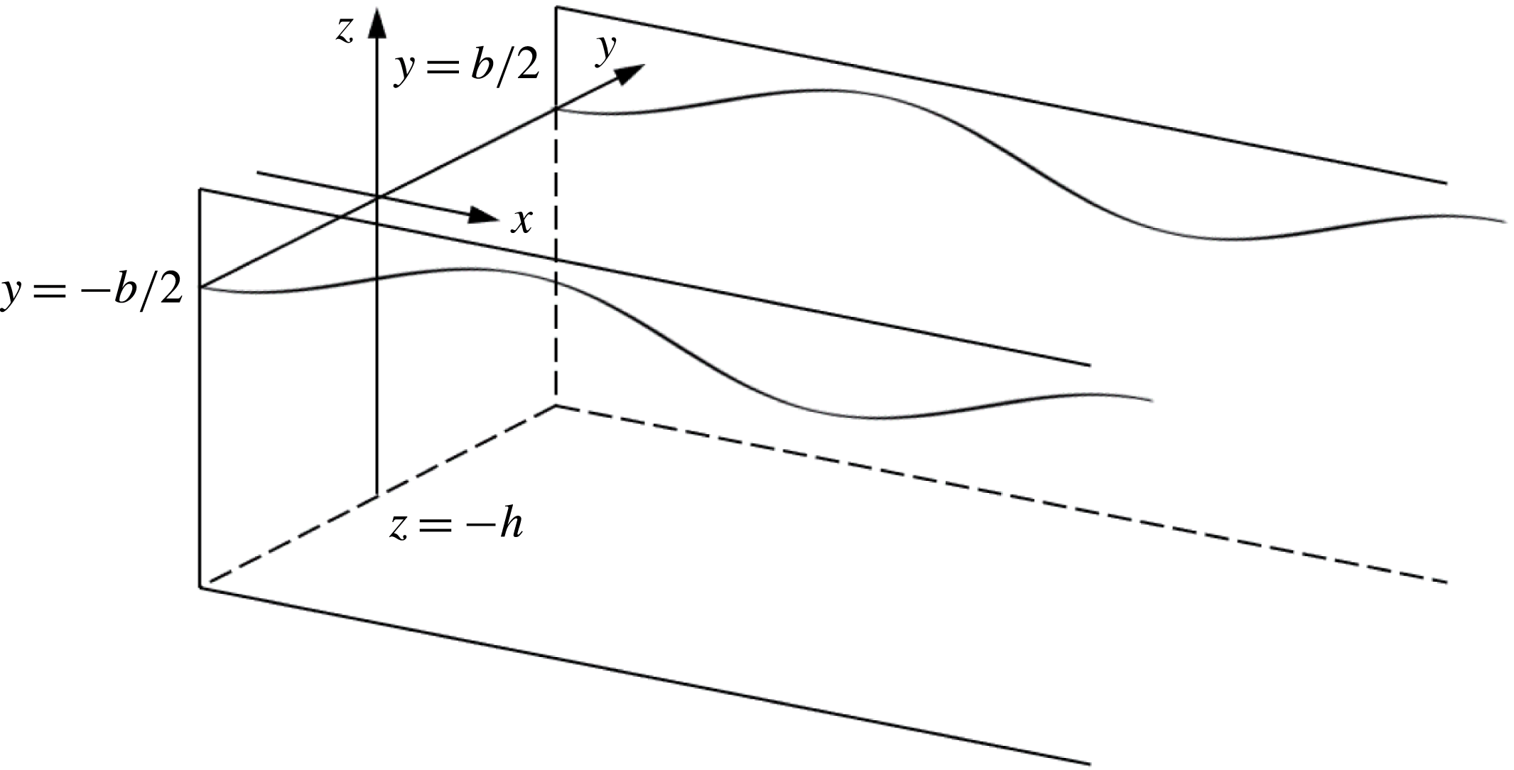
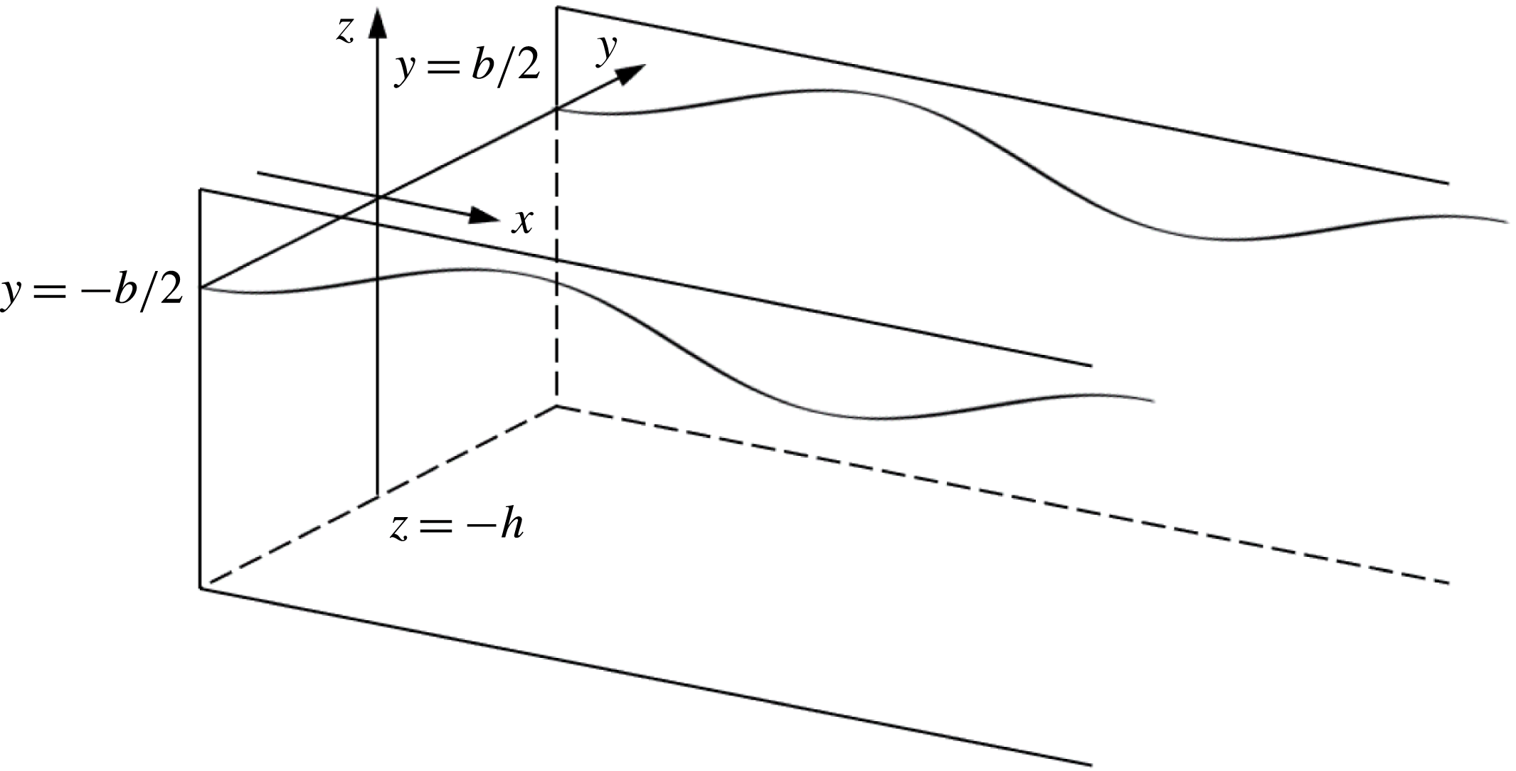
View of rectangular water channel and coordinate system.
2 Formulation of the problem
2.1 Characteristics of waves in a rectangular water channel
The aim of this section is to derive the characteristics of a small cross-joint water channel by circuit analysis. First, the characteristics of waves in a rectangular water channel are derived. Let us consider water waves propagating to the rectangular water channel with width
 $b$
. Figure 1 shows a view of the rectangular water channel. The origin of the coordinate system is placed on the undisturbed free surface. Incident waves propagate along the
 $x$
-axis, and the
 $z$
-axis is positive vertically upward. Side walls are located at
 $y=\pm b/2$
parallel to the
 $x$
-axis and the water depth is
 $z=-h$
. In order to analyse the linearized potential-flow problem, small amplitude incident waves and an incompressible and inviscid flow with irrotational motion are assumed. Then, the velocity potential,
 $\unicode[STIX]{x1D6F7}$
, is introduced. Under these conditions, the velocity potential satisfies the law of conservation of mass
 $$\begin{eqnarray}\displaystyle \unicode[STIX]{x1D6FB}^{2}\unicode[STIX]{x1D6F7}=0, & & \displaystyle\end{eqnarray}$$
where
 $\unicode[STIX]{x1D735}$
is a vector differential operator and
 $\unicode[STIX]{x1D6FB}^{2}=\unicode[STIX]{x1D735}\boldsymbol{\cdot }\unicode[STIX]{x1D735}$
is the Laplacian. Equation (2.1) is Laplace’s equation that dominates the fluid domain. To solve the boundary-value problem, boundary conditions should be taken into account as follows
 $$\begin{eqnarray}\displaystyle & \displaystyle [\text{F}]\frac{\unicode[STIX]{x2202}^{2}\unicode[STIX]{x1D6F7}}{\unicode[STIX]{x2202}t^{2}}+g\frac{\unicode[STIX]{x2202}\unicode[STIX]{x1D6F7}}{\unicode[STIX]{x2202}z}=0\quad \text{on }z=0, & \displaystyle\end{eqnarray}$$
 $$\begin{eqnarray}\displaystyle & \displaystyle [\text{B}]\frac{\unicode[STIX]{x2202}\unicode[STIX]{x1D6F7}}{\unicode[STIX]{x2202}z}=0\quad \text{at }z=-h, & \displaystyle\end{eqnarray}$$
 $$\begin{eqnarray}\displaystyle & \displaystyle [\text{S}]\frac{\unicode[STIX]{x2202}\unicode[STIX]{x1D6F7}}{\unicode[STIX]{x2202}y}=0\quad \text{at }y=\pm \frac{b}{2}, & \displaystyle\end{eqnarray}$$
where
 $g$
is the gravitational acceleration. Equation (2.2) is the linearized free surface condition on the free surface [F], equation (2.3) is the bottom condition at the bottom surface [B] and (2.4) is the side wall condition at the surface of the side wall [S]. The set of these equations is solved by the variable separation method. Velocity potential is separated with respect to each axis and is assumed to be sinusoidal in time as
 $$\begin{eqnarray}\displaystyle \unicode[STIX]{x1D6F7}(x,y,z;t)=Y(y)Z(z)\cos (\unicode[STIX]{x1D714}t-k_{x}x), & & \displaystyle\end{eqnarray}$$
where
 $\unicode[STIX]{x1D714}$
is the circular frequency and
 $k_{x}$
is the wavenumber for the
 $x$
direction. By substituting (2.5) into (2.1) with boundary conditions, we get
 $$\begin{eqnarray}\displaystyle \unicode[STIX]{x1D6F7}(x,y,z;t)=G\text{e}^{\text{i}(\unicode[STIX]{x1D714}t-k_{x}x)}\cos \left\{k_{y}\left(y+\frac{b}{2}\right)\right\}\cosh \{k_{z}(z+h)\}, & & \displaystyle\end{eqnarray}$$
where
 $G$
is a constant and
 $k_{y},k_{z}$
are the wavenumbers for the
 $y$
and
 $z$
directions. Wavenumbers satisfy the following conditions
 $$\begin{eqnarray}\displaystyle & \displaystyle k_{x}^{2}+k_{y}^{2}=k_{z}^{2}\equiv k^{2}, & \displaystyle\end{eqnarray}$$
 $$\begin{eqnarray}\displaystyle & \displaystyle k_{y}=\frac{n\unicode[STIX]{x03C0}}{b}\quad (n=0,1,2,\ldots ), & \displaystyle\end{eqnarray}$$
 $$\begin{eqnarray}\displaystyle & \displaystyle \frac{\unicode[STIX]{x1D714}^{2}}{g}=k_{z}\tanh k_{z}h, & \displaystyle\end{eqnarray}$$
where
 $n$
is the number of the wave mode.
In this paper, we in particular deal with the shallow water problem. When the water depth
 $h$
is sufficiently smaller than the wavelength
 $\unicode[STIX]{x1D706}$
, the long wave approximation is applicable. (
 $h/\unicode[STIX]{x1D706}\leqslant 1/20$
is a standard condition for which the error is less than 3 %.) Then, the wavenumbers become
 $$\begin{eqnarray}\displaystyle & \displaystyle k_{x}=\sqrt{\frac{\unicode[STIX]{x1D714}^{2}}{gh}-\left(\frac{n\unicode[STIX]{x03C0}}{b}\right)^{2}}, & \displaystyle\end{eqnarray}$$
 $$\begin{eqnarray}\displaystyle & \displaystyle k_{y}=\frac{n\unicode[STIX]{x03C0}}{b}, & \displaystyle\end{eqnarray}$$
 $$\begin{eqnarray}\displaystyle & \displaystyle k_{z}=k=\frac{\unicode[STIX]{x1D714}}{\sqrt{gh}}. & \displaystyle\end{eqnarray}$$
Phase velocity
 $c$
is also obtained as
 $$\begin{eqnarray}\displaystyle c=\sqrt{gh}. & & \displaystyle\end{eqnarray}$$
Equation (2.10) indicates that the waves propagate along the
 $x$
-axis only when the value in the square root is positive. Here,
 $\unicode[STIX]{x1D714}_{c}=\sqrt{gh}(n\unicode[STIX]{x03C0}/b)$
are cutoff frequencies which reduce energy flowing through the channel.
2.2 Equivalent electric circuit model to rectangular water channel
We consider designing wave fields in the water channels by an electric circuit model because circuit theory has an advantage in terms of designing its characteristics. Characteristics of waves propagating in a rectangular water channel can be expressed by the equivalent circuit (Mochizuki et al. Reference Mochizuki, Ando and Mitsuhashi1990). Particularly, a transmission line is introduced, which is an electric circuit taking length into consideration.
Let us describe an electric circuit density model, which is equivalent to the water channel per unit length. Considering the Euler equations and the continuity equation under the long wave approximation, the following equations are obtained
 $$\begin{eqnarray}\displaystyle \frac{\unicode[STIX]{x2202}P}{\unicode[STIX]{x2202}x}=-\text{i}\unicode[STIX]{x1D714}\unicode[STIX]{x1D70C}u,\quad \frac{\unicode[STIX]{x2202}u}{\unicode[STIX]{x2202}x}=-\!\left\{\text{i}\unicode[STIX]{x1D714}\frac{1}{\unicode[STIX]{x1D70C}gh}+\frac{1}{\text{i}\unicode[STIX]{x1D714}}\frac{1}{\unicode[STIX]{x1D70C}}\left(\frac{n\unicode[STIX]{x03C0}}{b}\right)^{2}\right\}P, & & \displaystyle\end{eqnarray}$$
 $$\begin{eqnarray}\displaystyle \frac{\unicode[STIX]{x2202}P}{\unicode[STIX]{x2202}y}=-\text{i}\unicode[STIX]{x1D714}\unicode[STIX]{x1D70C}v,\quad \frac{\unicode[STIX]{x2202}v}{\unicode[STIX]{x2202}y}=\frac{1}{\text{i}\unicode[STIX]{x1D714}}\frac{1}{\unicode[STIX]{x1D70C}}\left(\frac{n\unicode[STIX]{x03C0}}{b}\right)^{2}P, & & \displaystyle\end{eqnarray}$$
 $$\begin{eqnarray}\displaystyle \frac{\unicode[STIX]{x2202}P}{\unicode[STIX]{x2202}z}=-\text{i}\unicode[STIX]{x1D714}\unicode[STIX]{x1D70C}w,\quad \frac{\unicode[STIX]{x2202}w}{\unicode[STIX]{x2202}z}=\text{i}\unicode[STIX]{x1D714}\frac{1}{\unicode[STIX]{x1D70C}gh}P, & & \displaystyle\end{eqnarray}$$
where
 $P$
is the pressure,
 $(u,v,w)$
are components of the velocity vector
 $\boldsymbol{u}$
and
 $\unicode[STIX]{x1D70C}$
is the fluid density. Equations (2.14) to (2.16) are pair equations corresponding to telegraphic equations for each direction. Then, equivalent circuit models can be introduced for equations (2.14) to (2.16); however, it is much more complicated to deal with the higher wave modes
 $n>0$
, even by circuit analysis. Therefore, we only treat the progressive wave mode
 $n=0$
such that waves propagate along the
 $x$
-axis to simplify the problem. By defining the flow rate
 $Q=bhu$
, equation (2.14) is rewritten as
 $$\begin{eqnarray}\displaystyle \frac{\unicode[STIX]{x2202}P}{\unicode[STIX]{x2202}x}=-\text{i}\unicode[STIX]{x1D714}\frac{\unicode[STIX]{x1D70C}}{bh}Q,\quad \frac{\unicode[STIX]{x2202}Q}{\unicode[STIX]{x2202}x}=-\text{i}\unicode[STIX]{x1D714}\frac{b}{\unicode[STIX]{x1D70C}g}P, & & \displaystyle\end{eqnarray}$$
where the pressure
 $P$
and the flow rate
 $Q$
are sinusoidal functions in time. Equation (2.17) is equivalent to lossless circuit equations written as
 $$\begin{eqnarray}\displaystyle \frac{\unicode[STIX]{x2202}V}{\unicode[STIX]{x2202}x}=-\text{i}\unicode[STIX]{x1D714}L^{\prime }I,\quad \frac{\unicode[STIX]{x2202}I}{\unicode[STIX]{x2202}x}=-\text{i}\unicode[STIX]{x1D714}C^{\prime }V, & & \displaystyle\end{eqnarray}$$
where
 $V$
and
 $I$
are the voltage and the electric current,
 $L$
and
 $C$
are the inductance and the electric capacity and the superscript
 $^{\prime }$
denotes per unit length quantities which have the relations
 $L^{\prime }=L/\ell ,C^{\prime }=C/\ell$
, where
 $\ell$
is the unit length of the transmission line (or water channel). The lossless assumption corresponds to the wave mode
 $n=0$
and it is often used for transmission line metamaterials for designing the corresponding circuit models (e.g. Caloz & Itoh Reference Caloz and Itoh2002). Comparing (2.17) and (2.18), the following relations are obtained
 $$\begin{eqnarray}\displaystyle \left[P,Q,\frac{\unicode[STIX]{x1D70C}}{bh},\frac{b}{\unicode[STIX]{x1D70C}g}\right]\Longleftrightarrow [V,I,L^{\prime },C^{\prime }]. & & \displaystyle\end{eqnarray}$$
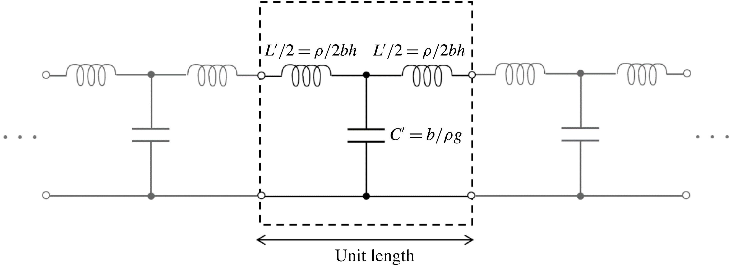
From this relations, we can write an equivalent electric circuit density model for the water channel as shown in figure 2. Characteristics of the water channel are obtained by circuit analysis as
 $$\begin{eqnarray}\displaystyle & \displaystyle Z_{0}=\sqrt{\frac{L^{\prime }}{C^{\prime }}}=\frac{\unicode[STIX]{x1D70C}}{b}\sqrt{\frac{g}{h}}, & \displaystyle\end{eqnarray}$$
 $$\begin{eqnarray}\displaystyle & \displaystyle \unicode[STIX]{x1D6FE}=\text{i}k=\text{i}\unicode[STIX]{x1D714}\sqrt{L^{\prime }C^{\prime }}=\frac{\text{i}\unicode[STIX]{x1D714}}{\sqrt{gh}}, & \displaystyle\end{eqnarray}$$
 $$\begin{eqnarray}\displaystyle & \displaystyle c=\frac{1}{\sqrt{L^{\prime }C^{\prime }}}=\sqrt{gh}, & \displaystyle\end{eqnarray}$$
where
 $Z_{0}$
is the characteristic impedance and
 $\unicode[STIX]{x1D6FE}$
is the propagation constant. We can see that the phase velocity
 $c$
obtained by the circuit analysis is equal to the one given by directly solving the shallow water wave problem as in (2.13).
Electric circuit density equivalent to water channel per unit length.

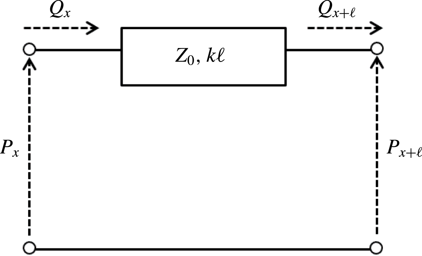
Transmission line with length
 $\ell$
equivalent to water channel.

The actual water channel has the dimension of length and thus equivalent circuit densities are connected in a cascade as in figure 2. Since it is cumbersome to cope with such cascaded circuits, the transmission line is introduced. Figure 3 shows the transmission line equivalent to the water channel with length
 $\ell$
. The transmission line is a type of linear system where input parameters
 $P_{x}$
and
 $Q_{x}$
are transferred to the outputs
 $P_{x+\ell }$
and
 $Q_{x+\ell }$
by a transfer function. To obtain the transfer function, let us consider the relation between the pressure and the flow rate at two points
 $x$
and
 $x+x^{\prime }$
with an arbitrary distance
 $x^{\prime }$
. Wave equations are obtained by (2.17) as
 $$\begin{eqnarray}\displaystyle \frac{\unicode[STIX]{x2202}^{2}P}{\unicode[STIX]{x2202}x^{2}}=-k^{2}P,\quad \frac{\unicode[STIX]{x2202}^{2}Q}{\unicode[STIX]{x2202}x^{2}}=-k^{2}Q. & & \displaystyle\end{eqnarray}$$
We assume trial functions as follows
 $$\begin{eqnarray}\displaystyle & \displaystyle P=P_{01}\text{e}^{\text{i}kx^{\prime }}+P_{02}\text{e}^{-\text{i}kx^{\prime }}, & \displaystyle\end{eqnarray}$$
 $$\begin{eqnarray}\displaystyle & \displaystyle Q=Q_{01}\text{e}^{\text{i}kx^{\prime }}+Q_{02}\text{e}^{-\text{i}kx^{\prime }}, & \displaystyle\end{eqnarray}$$
where
 $P_{01},P_{02},Q_{01}$
and
 $Q_{02}$
are unknown constants. Considering an initial condition
 $(P_{x},Q_{x})$
at point
 $x$
, solutions of (2.23) are determined as
 $$\begin{eqnarray}\displaystyle & \displaystyle P_{x+x^{\prime }}=P_{x}\cos kx^{\prime }-\text{i}Z_{0}Q_{x}\sin kx^{\prime }, & \displaystyle\end{eqnarray}$$
 $$\begin{eqnarray}\displaystyle & \displaystyle Q_{x+x^{\prime }}=-\frac{P_{x}}{Z_{0}}\sin kx^{\prime }+Q_{x}\cos kx^{\prime }. & \displaystyle\end{eqnarray}$$
The relation between distance
 $\ell$
in particular is written as
 $$\begin{eqnarray}\displaystyle \displaystyle \left(\begin{array}{@{}c@{}}P_{x}\\ P_{x+\ell }\end{array}\right)=-\text{i}Z_{0}\left(\begin{array}{@{}cc@{}}\cot k\ell & \csc k\ell \\ \csc k\ell & \cot k\ell \end{array}\right)\left(\begin{array}{@{}c@{}}Q_{x}\\ -Q_{x+\ell }\end{array}\right). & & \displaystyle\end{eqnarray}$$
The coefficient matrix which describes the relationship between the pressure and the flow rate (or voltage and current) is called the Z-parameter. Once we obtain the characteristic impedance
 $Z_{0}$
, the propagation constant
 $\unicode[STIX]{x1D6FE}=\text{i}k$
and distance
 $\ell$
, that is, once the width, depth and length of the water channel are determined, the characteristics at an arbitrary point are obtained.
The analogical design theory of the rectangular water channel described above was validated by an experiment (Mochizuki et al.
Reference Mochizuki, Ando and Mitsuhashi1990) and three-dimensional wave analysis (Kiyokawa & Mochizuki Reference Kiyokawa and Mochizuki1994). Both authors made a wave filter to prevent waves transmitting and both results show good agreement with the theory. The filter (Kiyokawa & Mochizuki Reference Kiyokawa and Mochizuki1994) also works for waves incident at angles
 $0^{\circ }$
–
 $30^{\circ }$
even though they also only consider the
 $n=0$
mode.
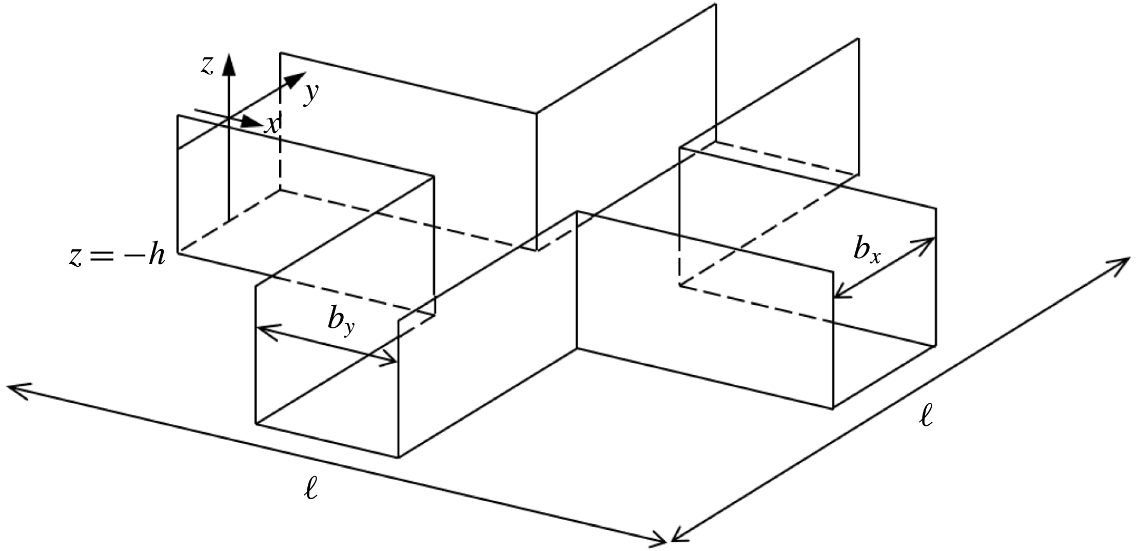
View of cross-joint rectangular water channel.

2.3 Equivalent electric circuit model to small cross-joint water channel
We extend circuit analysis of the water channel to the cross-joint rectangular water channel. Rectangular water channels with depth
 $h$
, widths
 $b_{x}$
and
 $b_{y}$
for each direction and length
 $\ell /2$
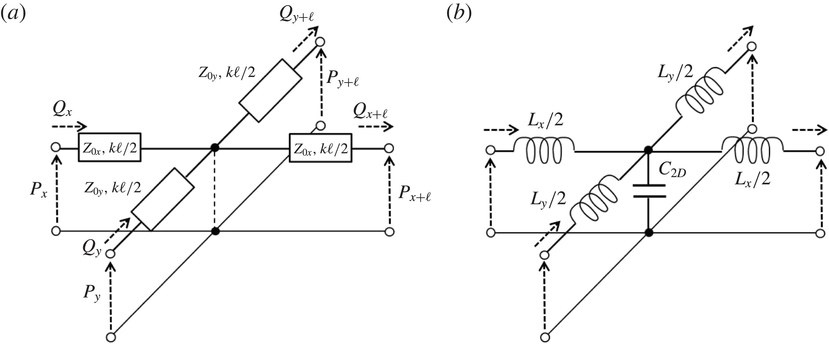
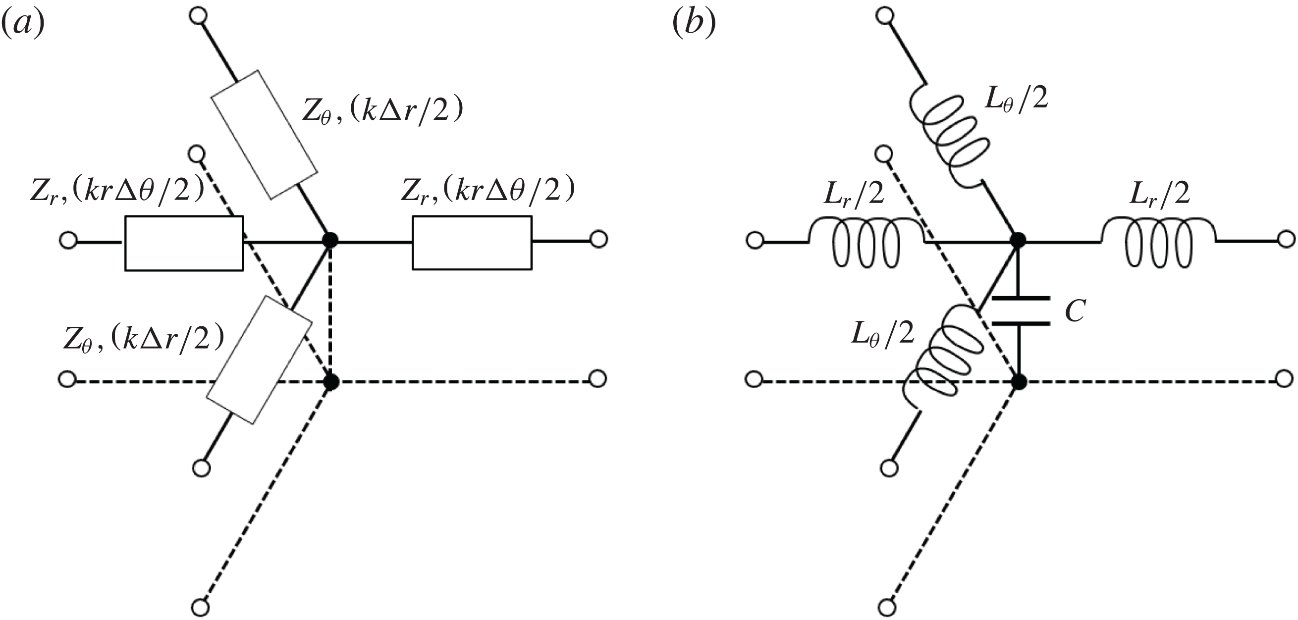
are jointed as shown in figure 4. The transmission line equivalent to this cross-joint water channel is written by the combination of a one-dimensional transmission line represented by figure 3 (even the length becomes half of its previous value), and this model is shown in figure 5(a). The relationship among pressures and flow rates is analytically obtained by Kirchhoff’s circuit laws through equation (2.28) with the use of the analogical relation of (2.19). Here, we only show the summarized result as follows
 $$\begin{eqnarray}\displaystyle \left(\begin{array}{@{}c@{}}P_{x}\\ P_{x+\ell }\\ P_{y}\\ P_{y+\ell }\end{array}\right)=\left(\begin{array}{@{}cccc@{}}A+B & B & B & B\\ B & A+B & B & B\\ B & B & D+B & B\\ B & B & B & D+B\end{array}\right)\left(\begin{array}{@{}c@{}}Q_{x}\\ -Q_{x+\ell }\\ Q_{y}\\ -Q_{y+\ell }\end{array}\right), & & \displaystyle\end{eqnarray}$$
where
 $$\begin{eqnarray}\displaystyle A=\text{i}Z_{0x}\tan \frac{k\ell }{2},\quad D=\text{i}Z_{0y}\tan \frac{k\ell }{2}, & & \displaystyle\end{eqnarray}$$
 $$\begin{eqnarray}\displaystyle B=\frac{\displaystyle Z_{0x}Z_{0y}\sec \frac{k\ell }{2}\csc \frac{k\ell }{2}}{2\text{i}(Z_{0x}+Z_{0y})}, & & \displaystyle\end{eqnarray}$$
 $$\begin{eqnarray}\displaystyle Z_{0x}=\frac{\unicode[STIX]{x1D70C}}{b_{x}}\sqrt{\frac{g}{h}},\quad Z_{0y}=\frac{\unicode[STIX]{x1D70C}}{b_{y}}\sqrt{\frac{g}{h}}. & & \displaystyle\end{eqnarray}$$
Note that equation (2.29) holds only when the depths and lengths of the
 $x$
and
 $y$
directions are equal (that is,
 $k_{x}\ell _{x}/2=k_{y}\ell _{y}/2=k\ell /2$
).
(a) Transmission line equivalent to cross-joint water channel. (b) Equivalent circuit model to (a).

In addition, the transmission line can be transformed into the equivalent circuit model as in figure 5(b). The relational expressions among pressures and flow rates in figure 5(b) are also obtained as
 $$\begin{eqnarray}\displaystyle \left(\begin{array}{@{}c@{}}P_{x}\\ P_{x+\ell }\\ P_{y}\\ P_{y+\ell }\end{array}\right)=\left(\begin{array}{@{}cccc@{}}\hat{A}+\hat{B} & \hat{B} & \hat{B} & \hat{B}\\ \hat{B} & \hat{A}+\hat{B} & \hat{B} & \hat{B}\\ \hat{B} & \hat{B} & \hat{D}+\hat{B} & \hat{B}\\ \hat{B} & \hat{B} & \hat{B} & \hat{D}+\hat{B}\end{array}\right)\left(\begin{array}{@{}c@{}}Q_{x}\\ -Q_{x+\ell }\\ Q_{y}\\ -Q_{y+\ell }\end{array}\right), & & \displaystyle\end{eqnarray}$$
where
 $$\begin{eqnarray}\displaystyle \hat{A}=\text{i}\unicode[STIX]{x1D714}\frac{L_{x}}{2},\quad \hat{D}=\text{i}\unicode[STIX]{x1D714}\frac{L_{y}}{2}, & & \displaystyle\end{eqnarray}$$
 $$\begin{eqnarray}\displaystyle \hat{B}=\frac{1}{\text{i}\unicode[STIX]{x1D714}C_{2D}}, & & \displaystyle\end{eqnarray}$$
 $L_{x}$
,
 $L_{y}$
and
 $C_{2D}$
are inductances and the capacity of the cross-joint water channel, and they are unknown coefficients. Comparing matrix coefficients between equations (2.29) and (2.33), we get
 $$\begin{eqnarray}\displaystyle L_{x}=\frac{2Z_{0x}}{\unicode[STIX]{x1D714}}\tan \frac{k\ell }{2},\quad L_{y}=\frac{2Z_{0y}}{\unicode[STIX]{x1D714}}\tan \frac{k\ell }{2} & & \displaystyle\end{eqnarray}$$
 $$\begin{eqnarray}\displaystyle C_{2D}=\frac{(Z_{0x}+Z_{0y})\sin k\ell }{\unicode[STIX]{x1D714}Z_{0x}Z_{0y}}. & & \displaystyle\end{eqnarray}$$
 $Z_{0x}$
,
 $Z_{0y}$
and
 $k\ell$
are calculated from the widths, depth and length of the water channel. Hence the characteristics of waves in the cross-joint water channel can be obtained.
Generally, the inductances and capacity are periodic functions as shown in (2.36) and (2.37). Here, we assume a very small water channel which is sufficiently smaller than the wavelength,
 $10\ell \leqslant \unicode[STIX]{x1D706}$
for instance. Then, trigonometric functions can be assumed as
 $\sin \unicode[STIX]{x1D703}=\tan \unicode[STIX]{x1D703}\approx \unicode[STIX]{x1D703}$
and
 $\cos \unicode[STIX]{x1D703}\approx 1$
. By using these approximations, equations (2.36) and (2.37) are deformed as
 $$\begin{eqnarray}\displaystyle L_{x}\approx \frac{Z_{0x}k\ell }{\unicode[STIX]{x1D714}}=\frac{\unicode[STIX]{x1D70C}\ell }{b_{x}h},\quad L_{y}\approx \frac{Z_{0y}k\ell }{\unicode[STIX]{x1D714}}=\frac{\unicode[STIX]{x1D70C}\ell }{b_{y}h}, & & \displaystyle\end{eqnarray}$$
 $$\begin{eqnarray}\displaystyle C_{2D}\approx \frac{(Z_{0x}+Z_{0y})k\ell }{\unicode[STIX]{x1D714}Z_{0x}Z_{0y}}=\frac{(b_{x}+b_{y})\ell }{\unicode[STIX]{x1D70C}g}. & & \displaystyle\end{eqnarray}$$
Hence, the inductances and capacity approximately approach definite values independent of the frequency. As a result, this small water channel works for a wide range of frequencies as long as the water channel and water depth can be treated as relatively small compared to the wavelength.
Finally, we consider the special case where the widths for the
 $x$
and
 $y$
directions hold the relation
 $b_{x}=b_{y}=b$
, namely, where an isotropic small water channel is designed. Characteristics of the small channel are then deformed as
 $$\begin{eqnarray}\displaystyle & \displaystyle L_{2D}\equiv L_{x}=L_{y}=\frac{\unicode[STIX]{x1D70C}\ell }{bh}, & \displaystyle\end{eqnarray}$$
 $$\begin{eqnarray}\displaystyle & \displaystyle C_{2D}=\frac{2b\ell }{\unicode[STIX]{x1D70C}g}. & \displaystyle\end{eqnarray}$$
Inductance
 $L_{2D}$
is same as the inductance of the unidirectional rectangular water channel. However, the capacity
 $C_{2D}$
doubles (see (2.19)). This is because the capacity at which a flow can pass through the small cross-joint channel becomes twice as much as the capacity of the unidirectional rectangular channel at the junction. Such a curious result is validated in electric waves and the details have been discussed in a book (Christopoulos Reference Christopoulos1995). Therefore, the characteristics of the small cross-joint channel are obtained as
 $$\begin{eqnarray}\displaystyle & \displaystyle Z_{2D}=\sqrt{\frac{L_{2D}^{\prime }}{C_{2D}^{\prime }}}=\frac{\unicode[STIX]{x1D70C}}{b}\sqrt{\frac{g}{2h}}=\frac{1}{\sqrt{2}}Z_{0}, & \displaystyle\end{eqnarray}$$
 $$\begin{eqnarray}\displaystyle & \displaystyle \unicode[STIX]{x1D6FE}_{2D}=\text{i}k_{2D}=\text{i}\unicode[STIX]{x1D714}\sqrt{L_{2D}^{\prime }C_{2D}^{\prime }}=\sqrt{2}\frac{\text{i}\unicode[STIX]{x1D714}}{\sqrt{gh}}=2\unicode[STIX]{x1D6FE}. & \displaystyle\end{eqnarray}$$
Similarly, phase velocity is given as
 $$\begin{eqnarray}\displaystyle c_{2D}=\frac{1}{\sqrt{2}}\sqrt{gh}=\frac{1}{\sqrt{2}}c. & & \displaystyle\end{eqnarray}$$
This indicates that waves in the small cross-joint water channel delay their phase velocity compared to waves in the unidirectional rectangular water channel (
 $c=\sqrt{gh}$
) due to the capacity at the cross-junction.
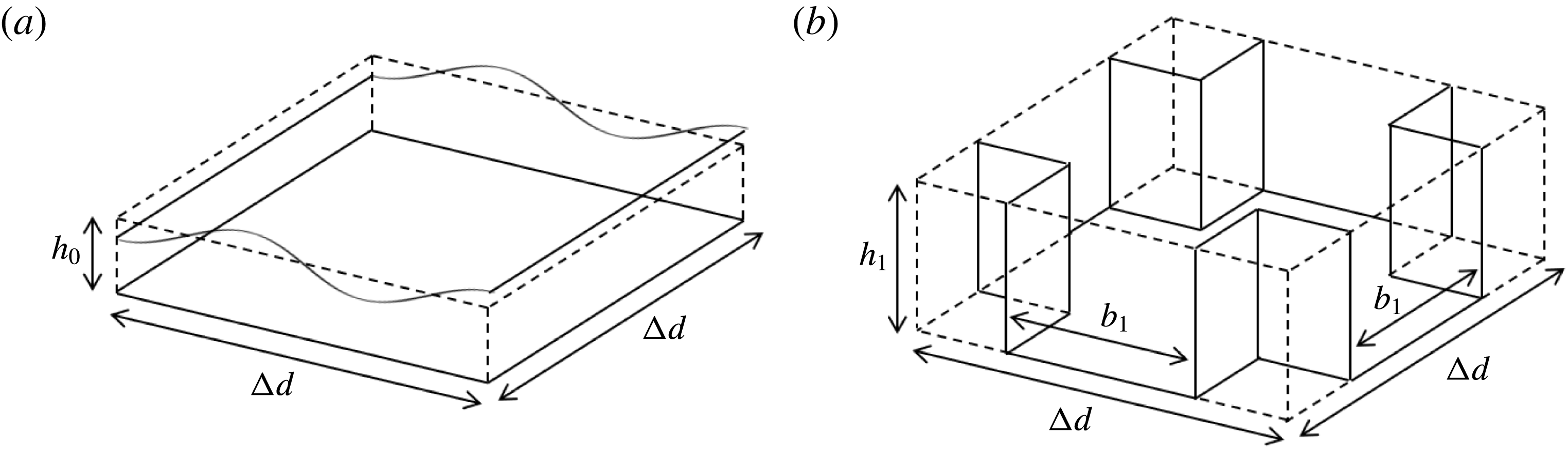
(a) Small space with size
 $\unicode[STIX]{x0394}d\times \unicode[STIX]{x0394}d\times h_{0}$
to which shallow water waves propagate. (b) Small water channel with width
 $b_{1}$
installed in the small space
 $\unicode[STIX]{x0394}d\times \unicode[STIX]{x0394}d\times h_{1}$
.

3 Isotropic small water channel network equivalent to shallow water with constant depth
3.1 Design of small water channel network
In order to confirm the proposed theory, an isotropic small water channel is designed to be equivalent to the shallow water space with constant depth
 $h_{0}$
. In particular, we focus on the small space of a shallow water domain with size
 $\unicode[STIX]{x0394}d\times \unicode[STIX]{x0394}d\times h_{0}$
as shown in figure 6(a). This domain is an open space, and waves seamlessly transfer to/from other domains through surrounding boundaries. Flow rates through cross-sections of the
 $x$
- and
 $y$
-axes are defined as
 $Q_{x}=\unicode[STIX]{x0394}dh_{0}u$
and
 $Q_{y}=\unicode[STIX]{x0394}dh_{0}v$
. Governing equations are obtained in the same way as the derivation of (2.17) and are shown as functions of the pressure and flow rates as
 $$\begin{eqnarray}\displaystyle & \displaystyle \frac{\unicode[STIX]{x2202}P}{\unicode[STIX]{x2202}x}=-\text{i}\unicode[STIX]{x1D714}\frac{\unicode[STIX]{x1D70C}}{\unicode[STIX]{x0394}dh_{0}}Q_{x}, & \displaystyle\end{eqnarray}$$
 $$\begin{eqnarray}\displaystyle & \displaystyle \frac{\unicode[STIX]{x2202}P}{\unicode[STIX]{x2202}y}=-\text{i}\unicode[STIX]{x1D714}\frac{\unicode[STIX]{x1D70C}}{\unicode[STIX]{x0394}dh_{0}}Q_{y}, & \displaystyle\end{eqnarray}$$
 $$\begin{eqnarray}\displaystyle & \displaystyle \frac{\unicode[STIX]{x2202}Q_{x}}{\unicode[STIX]{x2202}x}+\frac{\unicode[STIX]{x2202}Q_{y}}{\unicode[STIX]{x2202}y}=-\text{i}\unicode[STIX]{x1D714}\frac{\unicode[STIX]{x0394}d}{\unicode[STIX]{x1D70C}g}P. & \displaystyle\end{eqnarray}$$
This wave field is the isotropic space, and we make the small water channel equivalent to this field. We consider a small space with size
 $\unicode[STIX]{x0394}d\times \unicode[STIX]{x0394}d\times h_{1}$
and the small cross-joint water channel with width
 $b_{1}$
is arranged as shown in figure 6(b). The equivalent circuit model of this channel is given in figure 5(b). Therefore, inductances and capacity are obtained as
 $$\begin{eqnarray}\displaystyle & \displaystyle L_{2D}=\frac{\unicode[STIX]{x1D70C}\unicode[STIX]{x0394}d}{b_{1}h}, & \displaystyle\end{eqnarray}$$
 $$\begin{eqnarray}\displaystyle & \displaystyle C_{2D}=\frac{2b_{1}\unicode[STIX]{x0394}d}{\unicode[STIX]{x1D70C}g}. & \displaystyle\end{eqnarray}$$
This condition is satisfied when the water channel is smaller than the wavelength. Telegraphic equations are also derived by the equivalent circuit model of figure 6(b) as
 $$\begin{eqnarray}\displaystyle & \displaystyle \frac{\unicode[STIX]{x2202}P}{\unicode[STIX]{x2202}x}=-\text{i}\unicode[STIX]{x1D714}\frac{L_{2D}}{\unicode[STIX]{x0394}d}Q_{x}, & \displaystyle\end{eqnarray}$$
 $$\begin{eqnarray}\displaystyle & \displaystyle \frac{\unicode[STIX]{x2202}P}{\unicode[STIX]{x2202}y}=-\text{i}\unicode[STIX]{x1D714}\frac{L_{2D}}{\unicode[STIX]{x0394}d}Q_{y}, & \displaystyle\end{eqnarray}$$
 $$\begin{eqnarray}\displaystyle & \displaystyle \frac{\unicode[STIX]{x2202}Q_{x}}{\unicode[STIX]{x2202}x}+\frac{\unicode[STIX]{x2202}Q_{y}}{\unicode[STIX]{x2202}y}=-\text{i}\unicode[STIX]{x1D714}\frac{C_{2D}}{\unicode[STIX]{x0394}d}P. & \displaystyle\end{eqnarray}$$
Equations (3.6)–(3.8) are governing equations which represent waves propagating to the small cross-joint water channel.
Then, we design this small water channel to be equivalent to figure 6(a). By comparing equations (3.1)–(3.3) and (3.6)–(3.8), the following relations are obtained
 $$\begin{eqnarray}\displaystyle & \displaystyle b_{1}=\frac{\unicode[STIX]{x0394}d}{2}, & \displaystyle\end{eqnarray}$$
 $$\begin{eqnarray}\displaystyle & \displaystyle h_{1}=2h_{0}. & \displaystyle\end{eqnarray}$$
There are conditions for the small water channel to be equivalent to the shallow water space. The characteristic impedance and the phase velocity are determined as
 $$\begin{eqnarray}\displaystyle & \displaystyle Z_{1}=\frac{\unicode[STIX]{x1D70C}}{\unicode[STIX]{x0394}d}\sqrt{\frac{g}{h_{0}}}, & \displaystyle\end{eqnarray}$$
 $$\begin{eqnarray}\displaystyle & \displaystyle c_{1}=\sqrt{gh_{0}}. & \displaystyle\end{eqnarray}$$
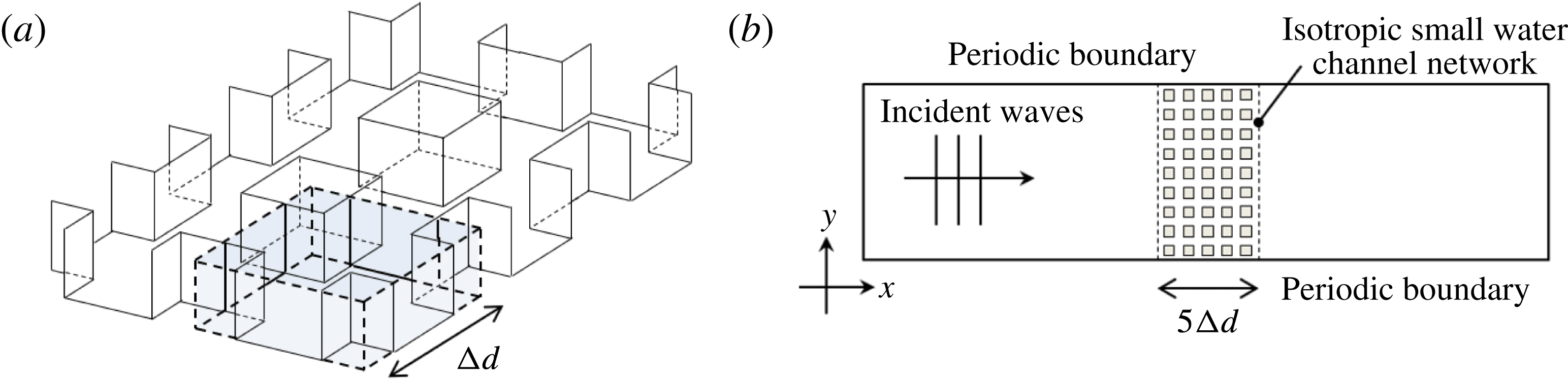
We can see that the impedance and phase velocity are matched between the small water channel and the small shallow water space. Since the impedance and the phase velocity of this water channel match with the open space, this water channel can be connected as a network. The image of the small water channel network is shown in figure 7(a).
(a) View of small water channel network. (b) Computation domain and boundaries.

3.2 Modelling and computation results
In order to validate the proposed equivalent model, numerical computations are carried out. We solve the three-dimensional boundary-value problem based on the linear potential theory represented by (2.1) with boundary conditions, and the assumption of the long wave approximation is not applied. We use COMSOL Multiphysics, a finite element method based software, to solve this problem. Figure 7(b) shows an image of the computational model. Equations (2.2)–(2.4) are chosen as the free surface, walls of the channel and the bottom boundaries, respectively. Waves are incident from left to right boundaries and other vertical boundaries have periodic conditions. The value of the water depth is
 $h_{0}=1.0~(\text{m})$
and the size of the small water channel is
 $\unicode[STIX]{x0394}d=4h_{0}=4.0~(\text{m})$
. The network, composed of
 $5\times 9$
small water channels designed to be equivalent, are arranged at the centre of the fluid domain.
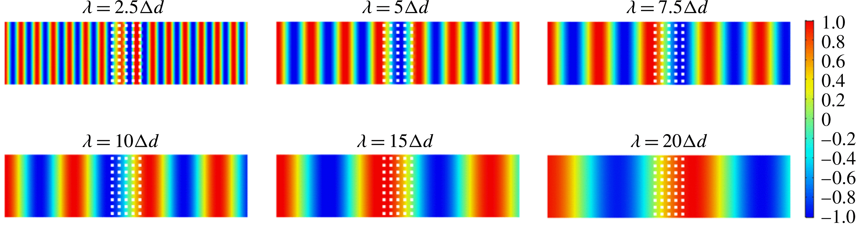
Wave patterns for wavelength
 $\unicode[STIX]{x1D706}$
equal
 $2.5\unicode[STIX]{x0394}d$
,
 $5\unicode[STIX]{x0394}d$
,
 $7.5\unicode[STIX]{x0394}d$
,
 $10\unicode[STIX]{x0394}d$
,
 $15\unicode[STIX]{x0394}d$
and
 $20\unicode[STIX]{x0394}d$
. An equivalent small water channel network is arranged in the centre domain.

Figure 8 shows the wave patterns for each wavelength. According to the results of
 $\unicode[STIX]{x1D706}=10\unicode[STIX]{x0394}d,15\unicode[STIX]{x0394}d$
and
 $20\unicode[STIX]{x0394}d$
, waves are not scattered when they are incident on an interface between the shallow water space and the small water channel network. Consequently, transmitted waves keep the form of the original incident waves. This is because the impedance of the wave fields in the small water channel network matches the impedance of the shallow water with a constant depth. In contrast, a few waves are reflected at the interface when the wavelength is not large enough, e.g.
 $\unicode[STIX]{x1D706}\leqslant 7.5\unicode[STIX]{x0394}d$
. Equations (3.11) and (3.12) are satisfied only when the size of the channel is sufficiently smaller than the wavelength. These computation results show good agreement with the proposed theory of the small water channel network.
Wave patterns of waves incident on the small water channel network at
 $15^{\circ }$
,
 $30^{\circ }$
and
 $45^{\circ }$
for
 $\unicode[STIX]{x1D706}=10\unicode[STIX]{x0394}d$
,
 $15\unicode[STIX]{x0394}d$
and
 $20\unicode[STIX]{x0394}d$
.

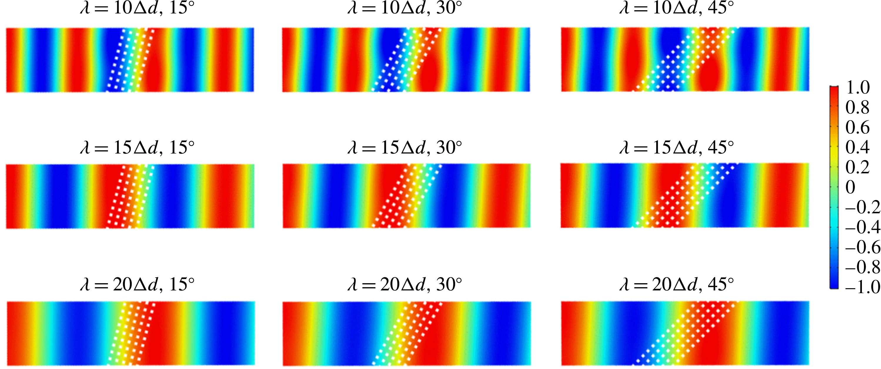
The proposed design method only considers progressive waves, which propagate to the network at right angles. On the other hand, the problem might be changed if waves have oblique angles. To investigate the validity of the proposed design, we have computed several cases where the waves are incident on the network at angles. We have tested some boundary conditions for upper and lower vertical boundaries; periodic, no flux (wall) and oblique inflow and outflow conditions. The result of the periodic condition is shown in figure 9. Figure 9 shows wave patterns with oblique angles
 $15^{\circ },30^{\circ }$
and
 $45^{\circ }$
for wavelengths
 $\unicode[STIX]{x1D706}=10\unicode[STIX]{x0394}d,15\unicode[STIX]{x0394}d$
and
 $20\unicode[STIX]{x0394}d$
, respectively. The results for
 $\unicode[STIX]{x1D706}=10$
indicate that wave deformations increase as the angles become bigger. On the other hand, the impedance seems to be matching if the wavelength
 $\unicode[STIX]{x1D706}$
is
 $15\unicode[STIX]{x0394}d$
or more. In spite of ignoring the higher wave modes, the small water channel network works well. These results correspond to the results by Kiyokawa & Mochizuki (Reference Kiyokawa and Mochizuki1994), even though they used unidirectional water channels and did not assume small channels. Note that the vertical boundaries can be bound by the periodic condition because the impedance matching is satisfied. When we use the wall condition or oblique inflow and outflow conditions, the network is only valid for smaller angles. It should also be noted that the scale of the small water channel itself is not so small, although the channels are relatively smaller than the wavelength. Since our target is free surface gravity-dominant waves in shallow water, capillary effects are not considered. We expect that the proposed design method might be applied to coastal engineering for the purpose of managing long waves.
4 Anisotropic small water channel network for realizing cloaking
4.1 Design of the small water channel network for cloaking
The design of an anisotropic small water channel is demonstrated by applying it to realize shallow water cloaking. Cloaking refers to a phenomenon that makes an object invisible. This study is influenced by Pendry et al. (Reference Pendry, Schurig and Smith2006), who proposed a method to deform the space for the sake of mimicking an object. As a result, waves propagate to detour the cloaked space and the object behaves as if it is invisible. The theory is originally based on the fact that Maxwell’s equations for electromagnetic waves are invariant under coordinate transformation. Nowadays, this idea is applied to several kinds of waves. We focus on the analogical method studied by Cummer & Schurig (Reference Cummer and Schurig2007), who compared the two-dimensional governing equations between electromagnetic and acoustic waves. Following their method, we can also analogize shallow water waves (vertically invariant two-dimensional water waves) to acoustic waves. Then, the governing equations, which are required to maintain the invariance under the transformation, are obtained as
 $$\begin{eqnarray}\displaystyle & \displaystyle \frac{\unicode[STIX]{x2202}P}{\unicode[STIX]{x2202}r}=-\text{i}\unicode[STIX]{x1D714}\frac{\unicode[STIX]{x1D70C}}{\unicode[STIX]{x1D70E}_{r}}u_{r}, & \displaystyle\end{eqnarray}$$
 $$\begin{eqnarray}\displaystyle & \displaystyle \frac{1}{r}\frac{\unicode[STIX]{x2202}P}{\unicode[STIX]{x2202}\unicode[STIX]{x1D703}}=-\text{i}\unicode[STIX]{x1D714}\frac{\unicode[STIX]{x1D70C}}{\unicode[STIX]{x1D70E}_{\unicode[STIX]{x1D703}}}u_{\unicode[STIX]{x1D703}}, & \displaystyle\end{eqnarray}$$
 $$\begin{eqnarray}\displaystyle & \displaystyle \frac{1}{r}\frac{\unicode[STIX]{x2202}}{\unicode[STIX]{x2202}r}(ru_{r})+\frac{1}{r}\frac{\unicode[STIX]{x2202}u_{\unicode[STIX]{x1D703}}}{\unicode[STIX]{x2202}\unicode[STIX]{x1D703}}=-\text{i}\unicode[STIX]{x1D714}\unicode[STIX]{x1D6FE}\frac{1}{\unicode[STIX]{x1D70C}gh_{0}}P, & \displaystyle\end{eqnarray}$$
where
 $$\begin{eqnarray}\displaystyle \unicode[STIX]{x1D748}\equiv \frac{\unicode[STIX]{x1D63C}\unicode[STIX]{x1D63C}^{\unicode[STIX]{x1D64F}}}{|\unicode[STIX]{x1D63C}|},\quad \unicode[STIX]{x1D6FE}\equiv \frac{1}{|\unicode[STIX]{x1D63C}|},\quad \unicode[STIX]{x1D748}_{cy}=\left(\begin{array}{@{}cc@{}}\unicode[STIX]{x1D70E}_{r} & 0\\ 0 & \unicode[STIX]{x1D70E}_{\unicode[STIX]{x1D703}}\end{array}\right). & & \displaystyle\end{eqnarray}$$
The original forms of (4.1) to (4.3) are obtained by transforming a shallow water continuity equation and Euler’s equations into a cylindrical system, and the additional coefficients detailed in (4.4) are the non-dimensional parameters which keep their original forms under the transformation.
 $\unicode[STIX]{x1D748}$
is the coefficient matrix represented in the Cartesian system and
 $\unicode[STIX]{x1D748}_{cy}$
denotes the form on the cylindrical coordinate system which is obtained by deforming
 $\unicode[STIX]{x1D748}$
to the cylindrical system.
 $\unicode[STIX]{x1D63C}$
is the Jacobian transformation matrix between the original and transformed coordinate systems, and superscript
 $\unicode[STIX]{x1D64F}$
represents the transposed matrix. Since
 $\unicode[STIX]{x1D748}_{cy}$
is represented by a diagonal matrix, dealing with the form in the cylindrical system is easier than that in the Cartesian grid.
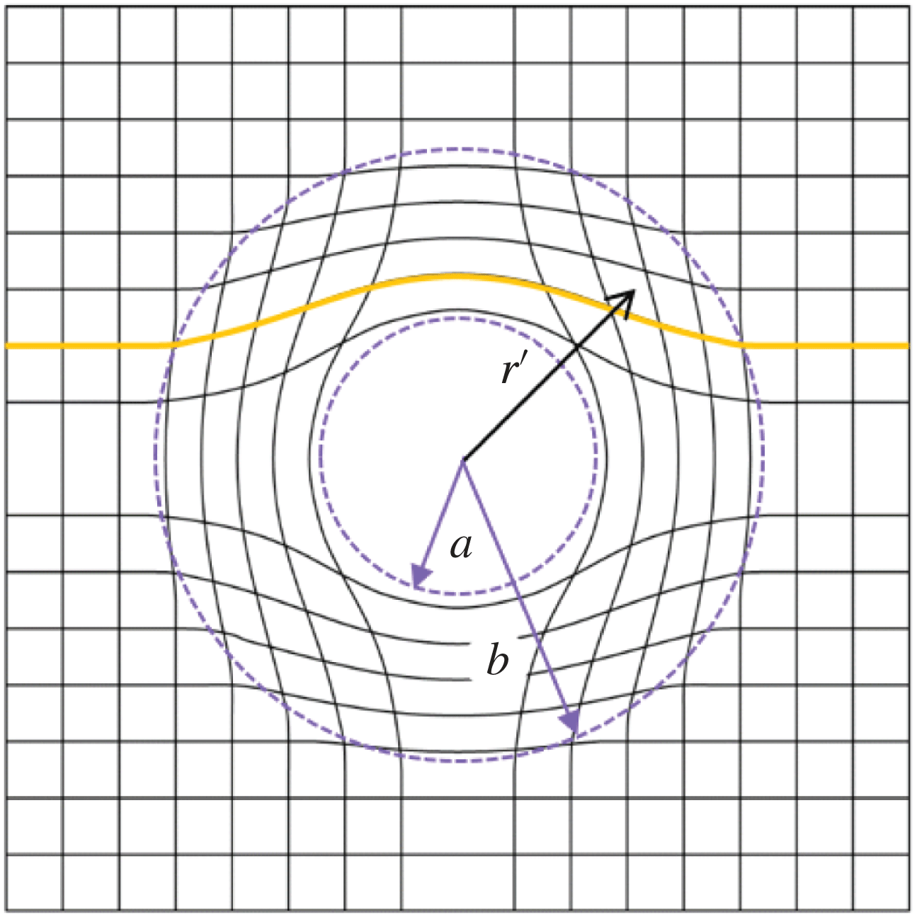
We particularly consider the coordinate transformation to compress a space from a cylindrical region to an annular region so as to cloak an object in the annulus
 $$\begin{eqnarray}\displaystyle r^{\prime }=\frac{b-a}{b}r+a,\quad \unicode[STIX]{x1D703}^{\prime }=\unicode[STIX]{x1D703},\quad z^{\prime }=z, & & \displaystyle\end{eqnarray}$$
where
 $(r,\unicode[STIX]{x1D703},z)$
denotes the original cylindrical coordinate system,
 $(r^{\prime },\unicode[STIX]{x1D703}^{\prime },z^{\prime })$
is a new system for cloaking and
 $a$
and
 $b$
are inner and outer radii of the cloaking region, respectively. This transformation is shown in figure 10. Then, the origin becomes a singular point that can cover the object. By substituting equation (4.5) into equation (4.4),
 $\unicode[STIX]{x1D748}_{cy}$
and
 $\unicode[STIX]{x1D6FE}$
are obtained as
 $$\begin{eqnarray}\displaystyle \unicode[STIX]{x1D70E}_{r}=\frac{r-a}{r},\quad \unicode[STIX]{x1D70E}_{\unicode[STIX]{x1D703}}=\frac{r}{r-a},\quad \unicode[STIX]{x1D6FE}=\frac{b^{2}}{(b-a)^{2}}\frac{r-a}{r}. & & \displaystyle\end{eqnarray}$$
In acoustic waves,
 $\unicode[STIX]{x1D748}_{cy}$
corresponds to the coefficients of the mass density
 $(\unicode[STIX]{x1D70C}_{r},\unicode[STIX]{x1D70C}_{\unicode[STIX]{x1D703}})$
and
 $\unicode[STIX]{x1D6FE}$
to the bulk modulus
 $\unicode[STIX]{x1D705}$
. Therefore, the acoustic cloaking domain can be modelled by using these three parameters. On the other hand, the shallow water governing equations do not have plenty of variables. Zareei & Alam (Reference Zareei and Alam2015) used the water depth
 $(h_{r},h_{\unicode[STIX]{x1D703}})$
and the gravitational acceleration
 $g$
as these variables; however, the gravitational acceleration
 $g$
cannot change practically, so that they introduced the nonlinear transformation to reduce the number of variables, and the gravity remains constant. Berraquero et al. (Reference Berraquero, Maurel, Petitjeans and Pagneux2013) also utilized such a feasible transformation with a condition
 $|\unicode[STIX]{x1D63C}|=1$
for a water wave shifter.
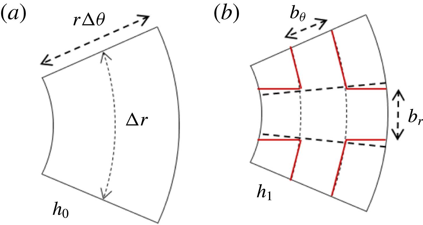
Here, we propose the use of the small water channel network to increase the feasible variables; the widths and depth of the cross-joint channel correspond to the three variables. Attention is now focused, as shown in figure 11(a), on a micro-section with
 $\unicode[STIX]{x0394}r\times r\unicode[STIX]{x0394}\unicode[STIX]{x1D703}\times h_{0}$
, that is selected to satisfy the condition
 $\unicode[STIX]{x0394}r=r\unicode[STIX]{x0394}\unicode[STIX]{x1D703}$
for every radius in the cylindrical system. We pick up the micro-section and the flow rates
 $Q_{r}$
, and
 $Q_{\unicode[STIX]{x1D703}}$
are introduced. Then, equations (4.1)–(4.3) are rewritten as
 $$\begin{eqnarray}\displaystyle & \displaystyle \frac{\unicode[STIX]{x2202}P}{\unicode[STIX]{x2202}r}=-\text{i}\unicode[STIX]{x1D714}\frac{1}{\unicode[STIX]{x1D70E}_{r}}\frac{\unicode[STIX]{x1D70C}}{\unicode[STIX]{x0394}rh_{0}}Q_{r}, & \displaystyle\end{eqnarray}$$
 $$\begin{eqnarray}\displaystyle & \displaystyle \frac{1}{r}\frac{\unicode[STIX]{x2202}P}{\unicode[STIX]{x2202}\unicode[STIX]{x1D703}}=-\text{i}\unicode[STIX]{x1D714}\frac{1}{\unicode[STIX]{x1D70E}_{\unicode[STIX]{x1D703}}}\frac{\unicode[STIX]{x1D70C}}{\unicode[STIX]{x0394}rh_{0}}Q_{\unicode[STIX]{x1D703}}, & \displaystyle\end{eqnarray}$$
 $$\begin{eqnarray}\displaystyle & \displaystyle \frac{1}{r}\frac{\unicode[STIX]{x2202}}{\unicode[STIX]{x2202}r}(rQ_{r})+\frac{1}{r}\frac{\unicode[STIX]{x2202}Q_{\unicode[STIX]{x1D703}}}{\unicode[STIX]{x2202}\unicode[STIX]{x1D703}}=-\text{i}\unicode[STIX]{x1D714}\unicode[STIX]{x1D6FE}\frac{\unicode[STIX]{x0394}r}{\unicode[STIX]{x1D70C}g}P. & \displaystyle\end{eqnarray}$$
Equation (4.9) is given only when
 $\unicode[STIX]{x0394}r=r\unicode[STIX]{x0394}\unicode[STIX]{x1D703}$
. To satisfy equations (4.7)–(4.9), we arrange the anisotropic small water channel network as shown in figure 11(b), where
 $b_{r}$
and
 $b_{\unicode[STIX]{x1D703}}$
are the widths of each direction and
 $h_{1}$
is the depth of the channel. Dotted line shows a model of an ideal cylindrical water channel. In fact, it is difficult to analyse this cylindrical channel by taking into account the width spreading distance
 $r$
and curving. Therefore, such forms are ignored in designing the circuit model, and a connection of rectangular water channels is assumed. A solid line shows the shape of this rectangular water channel, and the transmission line and equivalent circuit model of this water channel are shown in figure 12. As shown in figures 11 and 12, water channels and circuit models for the radial and azimuth directions are actually connected slantwise. Since this oblique angle is small, we assume it is a right angle. Therefore, the circuit model of this water channel is treated as the simple models shown in figure 5.
Coordinate transformation for cloaking.

(a) Small section of shallow water domain which holds
 $\unicode[STIX]{x0394}r=r\unicode[STIX]{x0394}\unicode[STIX]{x1D703}$
. (b) View of small water channel arranged in micro-section; dotted line shows ideal cylindrical model and solid line represents approximate channel model which is used for theory construction.

(a) Transmission line of anisotropic water channel for cloaking. (b) Equivalent circuit model to (a). Energy spread, curving and slantwise connection at junction are ignored.

Telegraphic equations are obtained from the equivalent circuit model as
 $$\begin{eqnarray}\displaystyle & \displaystyle \frac{\unicode[STIX]{x2202}P}{\unicode[STIX]{x2202}r}=-\text{i}\unicode[STIX]{x1D714}\frac{L_{r}}{\unicode[STIX]{x0394}r}Q_{r}, & \displaystyle\end{eqnarray}$$
 $$\begin{eqnarray}\displaystyle & \displaystyle \frac{1}{r}\frac{\unicode[STIX]{x2202}P}{\unicode[STIX]{x2202}\unicode[STIX]{x1D703}}=-\text{i}\unicode[STIX]{x1D714}\frac{L_{\unicode[STIX]{x1D703}}}{\unicode[STIX]{x0394}r}Q_{\unicode[STIX]{x1D703}}, & \displaystyle\end{eqnarray}$$
 $$\begin{eqnarray}\displaystyle & \displaystyle \frac{\unicode[STIX]{x2202}}{\unicode[STIX]{x2202}r}Q_{r}+\frac{1}{r}\frac{\unicode[STIX]{x2202}Q_{\unicode[STIX]{x1D703}}}{\unicode[STIX]{x2202}\unicode[STIX]{x1D703}}=-\text{i}\unicode[STIX]{x1D714}\frac{C}{\unicode[STIX]{x0394}r}P, & \displaystyle\end{eqnarray}$$
where
 $$\begin{eqnarray}\displaystyle L_{r}=\frac{\unicode[STIX]{x1D70C}\unicode[STIX]{x0394}r}{b_{r}h_{1}},\quad L_{\unicode[STIX]{x1D703}}=\frac{\unicode[STIX]{x1D70C}\unicode[STIX]{x0394}r}{b_{\unicode[STIX]{x1D703}}h_{1}}, & & \displaystyle\end{eqnarray}$$
 $$\begin{eqnarray}\displaystyle C=\frac{\unicode[STIX]{x0394}r(b_{r}+b_{\unicode[STIX]{x1D703}})}{\unicode[STIX]{x1D70C}g}, & & \displaystyle\end{eqnarray}$$
where the inductances and the capacity are given by (2.38) and (2.39). Note that the energy spread is ignored in (4.12). Equations (4.10)–(4.12) are the governing equations of this small water channel and its parameters are designed to be equivalent to equations (4.7)–(4.9). Comparing these equations, the widths and depth are finally determined as
 $$\begin{eqnarray}\displaystyle & \displaystyle b_{r}=\left(\frac{b}{b-a}\right)^{2}\frac{(r-a)^{3}}{((r-a)^{2}+r^{2})r}\unicode[STIX]{x0394}r, & \displaystyle\end{eqnarray}$$
 $$\begin{eqnarray}\displaystyle & \displaystyle b_{\unicode[STIX]{x1D703}}=\left(\frac{b}{b-a}\right)^{2}\frac{r(r-a)}{(r-a)^{2}+r^{2}}\unicode[STIX]{x0394}r, & \displaystyle\end{eqnarray}$$
 $$\begin{eqnarray}\displaystyle & \displaystyle h_{1}=\left(\frac{b-a}{b}\right)^{2}\frac{(r-a)^{2}+r^{2}}{(r-a)^{2}}h_{0}. & \displaystyle\end{eqnarray}$$
These parameters are given regardless of frequency and the restrictions of this theory are the long wave condition (
 $\unicode[STIX]{x1D706}\gg h$
) and the small water channel condition (
 $\unicode[STIX]{x1D706}\gg \unicode[STIX]{x0394}r$
). Therefore, the proposed theory is valid as long as these conditions are satisfied. It should be noted that the depth
 $h_{1}$
approaches infinity at
 $r=a$
and the long wave condition cannot be fully satisfied. Practically, widths also have to meet the condition where widths are smaller than the length of micro-section (
 $b_{r},b_{\unicode[STIX]{x1D703}}<\unicode[STIX]{x0394}r$
). This transmission line model is implemented for diagonal anisotropy. The transmission line model for extension of the full tensor anisotropy with non-diagonal elements is shown in Nagayama & Sanada (Reference Nagayama and Sanada2015).
4.2 Modelling and computation results
We design the small water channel network to make a wave field equivalent to cloaking. In order to reduce time cost for computation, only the unilateral domain is considered. Initial parameters are carefully determined to satisfy the constraint conditions. We choose the water depth
 $h_{0}=1.0~(\text{m})$
and inner radius
 $a=10.0~(\text{m})$
. The semicircular cloaking domain is divided into
 $N_{\unicode[STIX]{x1D703}}=30$
channels in the azimuthal direction (
 $\unicode[STIX]{x0394}\unicode[STIX]{x1D703}=\unicode[STIX]{x03C0}/30$
). The outer radius
 $b$
and number of channels in the radial direction
 $N_{r}$
are selected so as to satisfy
 $\unicode[STIX]{x0394}r=r\unicode[STIX]{x0394}\unicode[STIX]{x1D703}$
and
 $b_{\unicode[STIX]{x1D703}}/\unicode[STIX]{x0394}r<1.0$
. Then, the outer radius
 $b=35.18~(\text{m})$
is determined with 12 channels for the radial direction. In total,
 $N_{\unicode[STIX]{x1D703}}\times N_{r}=360$
channels are considered. The maximum
 $\unicode[STIX]{x0394}r$
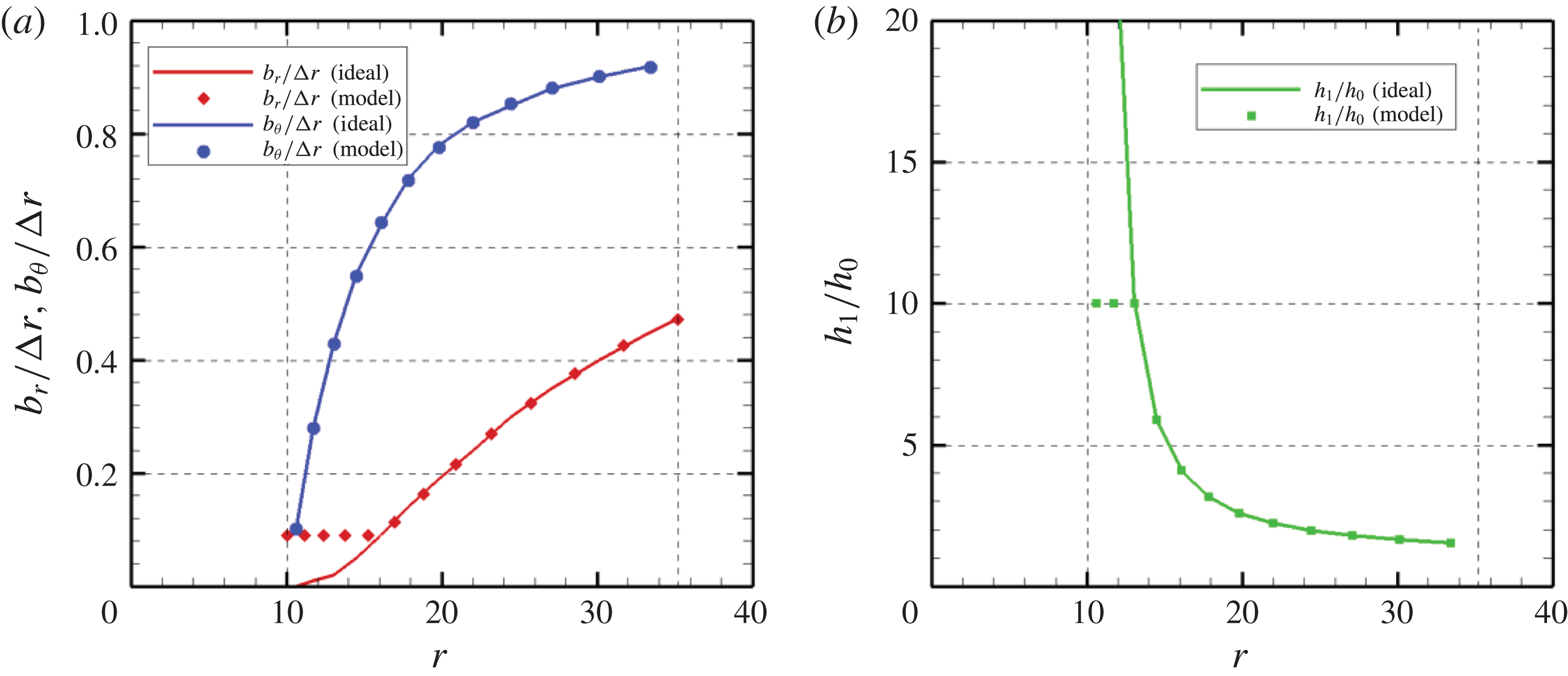
is 3.89 (m) on the outermost layer. The parameters of each channel are given by (4.15)–(4.17), and non-dimensional values are shown in figure 13. Figure 13(a) shows the widths
 $b_{r}$
and
 $b_{\unicode[STIX]{x1D703}}$
normalized by the size
 $\unicode[STIX]{x0394}r$
and figure 13(b) shows the depth
 $h_{1}$
per fundamental depth
 $h_{0}$
. Solid lines represent ideal values and symbols are feasible parameters for modelling. As the radius shortens, the relative widths become smaller. In contrast, depth diverges to infinity on the innermost layer. Widths are selected due to the limitation of the mesh modelling and the water depth is chosen to keep the long wave approximation.
(a) Widths of the small water channel network normalized by the size
 $\unicode[STIX]{x0394}r$
along the radius. (b) Depth normalized by constant depth
 $h_{0}$
. Solid lines show theoretical values and symbols are parameters for practical implementations.

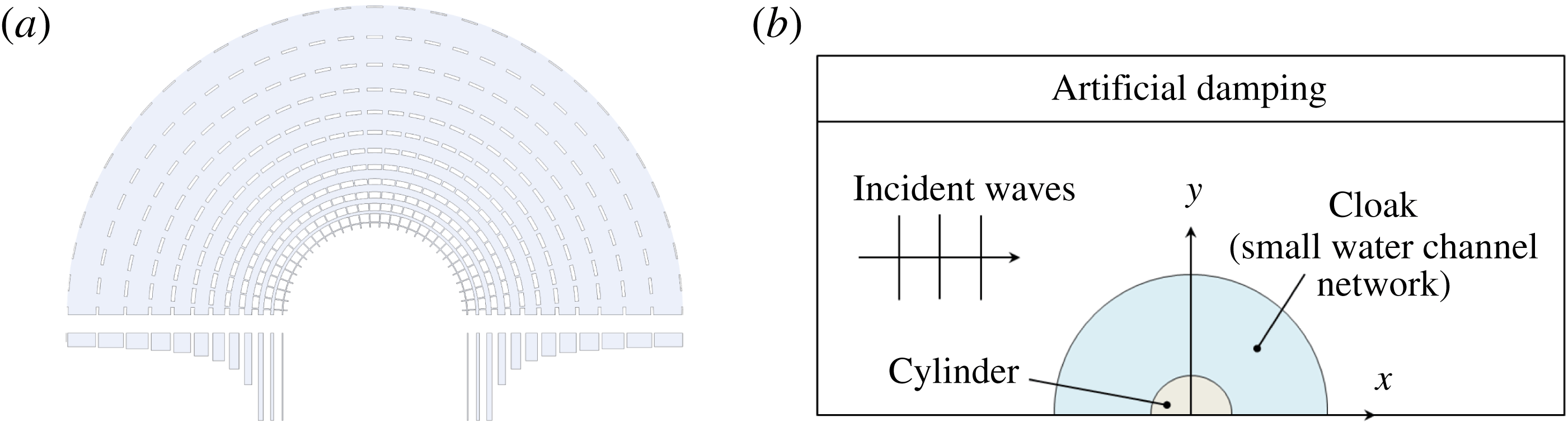
By using these parameters, the small water channel network is fashioned. Figure 14(a) shows top and side views of the small water channel network. Fluid domains of the channel are shown in light blue and blank domains represent walls. The width spreading along the radius was ignored to construct the circuit model; however, it is reconsidered to design the model. Figure 14(b) shows a computational domain. For numerical computations, the three-dimensional boundary-value problem is solved similar to § 3. Waves are incident from the left inflow boundary, and go out to the right outflow boundary. Artificial damping is applied for the top domain to reduce wave reflections. The bottom mounted cylinder is arranged at the centre and the small water channel network is arranged so as to cloak the cylinder.
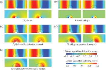
Resultant wave patterns are shown in figure 15. Each panel is composed of four figures. Figures above are diffraction waves which are superpositions of incident waves and scattering waves, and figures below are scattering wave patterns. Note that the colour legends are different for the upper figures
 $[-1.0,1.0]$
and the lower figures
 $[-0.2,0.2]$
for visualization. Left-hand figures are results of the wavelength
 $\unicode[STIX]{x1D706}=200~(\text{m})$
and right-hand figures are of the wavelength
 $\unicode[STIX]{x1D706}=240~(\text{m})$
.
(a) Top and side views of small water channel network for cloaking. Light blue colour represents fluid domain. (b) Modelling of computation domain and boundaries.

Wave patterns obtained by numerical computations. Each panel is composed of four figures; patterns above show diffraction waves which are superpositions of incident and scattering waves with colour legend
 $[-1.0,1.0]$
normalized by the incident wave amplitude, patterns below are scattering waves with colour legend
 $[-0.2,0.2]$
. Figures on the left are the case of wavelength
 $\unicode[STIX]{x1D706}=200~(\text{m})$
and the right figures are of
 $\unicode[STIX]{x1D706}=240~(\text{m})$
. (a) Wave pattern around the cylinder. (b) Ideal cloaking assuming virtual anisotropic fluid. (c) Cylinder surrounded by equivalent small water channel network. (d) Cloaking by anisotropic small water channel network. (e) Equivalent small water channel network as reference network model.

Figure 15(a) shows waves around the bottom mounted cylinder. Incident waves are scattered by the cylinder, although the wavelengths are very large. To cloak the cylinder and reduce scattering of waves, we assume an anisotropic virtual fluid represented by (4.6) surrounds the cylinder. This result is shown in figure 15(b). Waves detour to avoid the cylinder through the virtual fluid and therefore no wave is scattered as outgoing waves. This cloaking is valid regardless of the frequency because the parameters in (4.6) are independent of the frequency.
In order to realize this ideal cloaking, the small water channel network is designed. First, we design a reference channel model equivalent to the shallow water space with constant depth in the same manner as § 3. Choosing width
 $b_{r}=b_{\unicode[STIX]{x1D703}}=\unicode[STIX]{x0394}r/2$
and
 $h_{1}=2h_{0}$
, the impedance approximately matches at the interface. The results of the equivalent network model are shown in figure 15(e). The item of
 $\unicode[STIX]{x1D706}=200~(\text{m})$
in figure 15(e) indicates that shadow occurs behind the cylinder and the channel does not work equivalently to the shallow space even if the wavelengths are very large compared to the maximum size of the channel
 $(\unicode[STIX]{x1D706}=200~(\text{m})\gg \unicode[STIX]{x0394}r_{max}=3.89~(\text{m}))$
. On the other hand, the
 $\unicode[STIX]{x1D706}=240~(\text{m})$
point shows a seemingly good wave pattern although a few waves are still scattered by the reference network. The rectangular water channel network as in § 3 works if the wavelength is 10 times larger than the size of the channel; however, the cylindrical water channel requires a stricter condition, e.g.
 $\unicode[STIX]{x1D706}>60\unicode[STIX]{x0394}r_{max}\approx 240~(\text{m})$
, due to some assumptions we consider for the cylindrical system. We have tested some cases to investigate the validity of this equivalent model, such as by changing the size of the inner circular domain and the angle of channel connection (the number of discretizations for the azimuth direction), and
 $\unicode[STIX]{x1D706}>60\unicode[STIX]{x0394}r_{max}$
is required for all cases. This equivalent network is arranged around the cylinder and these results are shown in figure 15(c). Scattering waves for this case look like summations of the scattering waves of the cylinder (figure 15
a) and of the equivalent network (figure 15
e). We find that the diffraction waves at
 $\unicode[STIX]{x1D706}=240~(\text{m})$
are very close to those of figure 15(a).
Figure 15(d) shows the wave patterns by arranging the anisotropic network to cloak the cylinder. Similar to figure 15(c), a few waves are scattered on the outside of the network due to the existence of the channel itself, as shown in figure 15(e). These waves are caused regardless of the design of the channel. On the other hand, scattering waves generated by the cylinder can be suppressed especially in front of the cylinder. Consequently, diffraction waves show good agreement with waves of the ideal cloaking in figure 15(b). We cannot qualitatively discuss the achievement level of the cloaking because the scattered wave energy in the far field, which is usually used to estimate the cloaking, is very small due to the long wave restriction. The tendency of the cloaking, phase delays in front of the cylinder and rapid movement behind the cylinder, are well realized in the anisotropic network. The channel design is only valid for a progressive wave with wave mode
 $n=0$
, and therefore this channel network cannot achieve perfect cloaking. However, the effects of the higher wave modes do not appear to be high, and this model can approximate cloaking. Scattering waves by the cylinder can also be reduced even at
 $\unicode[STIX]{x1D706}=200~(\text{m})$
and therefore we believe that this discretization is sufficient for cloaking. In fact, a reduction in the number of discretizations requires a larger
 $b$
and
 $\unicode[STIX]{x0394}r_{max}$
, and then the valid wavelength becomes larger. The most dominant restriction of this proposed method is the use of the cylindrical water channel itself. If we use the rectangular channel as in § 3, such conditions might be mitigated, although it requires non-diagonal anisotropy to realize cylindrical cloaking.
5 Conclusions
We have proposed the use of a metamaterial with a small water channel network for designing wave fields in shallow water, and it is applied to attain water wave cloaking. The analytical solution of waves in the small water channel is derived by analogizing waves in a water channel to waves in an electric circuit. Using this analogy, the approach of the transmission line metamaterial is extended to metamaterials for water waves and the water channel is used as an alternative for the transmission line. We assume the size of the water channel is sufficiently smaller than the wavelength and a number of the channels are periodically connected as a network. By changing the widths and depth of each water channel of the network, the wave fields are artificially designed. Since the channel is small, the characteristics of the channel are decided as definite values and thus the proposed theory works for a wide range of frequency bands.
In order to validate the proposed method, we first design the isotropic water channel network to be equivalent to the shallow water space with constant depth. Choosing half the widths and twice the depth of the micro-section for the parameters of the water channel, the impedance and the phase velocity become equivalent to the shallow water space. Numerical computations are carried out and the isotropic network works when the wavelength is over 10 times larger than the size of the channel. We also compute oblique cases where waves are incident on the network at angles and the network still works if the wavelength is 15 times larger than the channel.
After that, the proposed design method is applied to designing an anisotropic small water channel network for demonstrating shallow water wave cloaking. We use cylindrical water channels, and the design parameters of the channels are analytically obtained by circuit analysis. A reference channel model, which is equivalent to a shallow water space with constant depth, is first designed in the same manner as the rectangular one. However, numerical results show that the model seemingly works only when the wavelength is 60 times bigger than the channel. An anisotropic network is also modelled and arranged to surround the cylinder. Computation results show that scattering waves from the cylinder can be reduced by the anisotropic network, and this network cloaks the cylinder well.
Acknowledgement
This work was supported by JSPS KAKENHI grant no JP16J00369.