3.1. Numerical methods

The mean velocity profiles used for resolvent analysis are all obtained from direct numerical simulations (DNS). These simulations use a staggered second-order finite difference scheme (Orlandi Reference Orlandi2000), with a fractional step method (Kim & Moin Reference Kim and Moin1985) and third-order Runge–Kutta time-advancing scheme (Wray Reference Wray1990). Further details regarding the use and validations of these methods, and their application to the specific cases considered here, can be found in Bae et al. (Reference Bae, Lozano-Duran, Bose and Moin2018, Reference Bae, Lozano-Durán, Bose and Moin2019) and Lozano-Durán & Bae (Reference Lozano-Durán and Bae2019).

For resolvent analysis, the wall-normal direction is discretised using a Chebyshev collocation method. In the cases where the spanwise dimension is explicitly discretised, we use a Fourier discretisation scheme with periodic boundary conditions along the spanwise domain. Moreover, if homogeneity is not assumed in the temporal dimension, we adopt a Fourier discretisation scheme when the system is assumed to be statistically stationary or time periodic (i.e. §§ 3.2–3.4), and an explicit Euler finite-differentiation scheme in the temporal dimension with Neumann boundary conditions at the boundaries in § 3.5. The corresponding differentiation operators for both Chebyshev and Fourier discretisations are defined according to the specifications given in Weideman & Reddy (Reference Weideman and Reddy2000). The number of collocation points used for each of the examples considered in this work will be indicated in the corresponding section. In each case, we verify that the numerical resolution gives converged results, with details of these convergence studies given in Appendix B.

In the space–time implementations of the analysis showcased in this paper (i.e. §§ 3.3–3.5), no-slip and no-penetration conditions are enforced at $y=0$ (lower wall), while free-slip and no-penetration conditions are enforced at $y=h$ (the channel centreline). The space–time analysis identifies modes that are sufficiently localised away from the mid-plane using the chosen set of parameters, allowing us to reduce the size of the numerical domain to the area below $y/h=1$.

3.2. Spatially sparse resolvent analysis of turbulent channel flow

Here, we apply the sparse resolvent analysis methodology on a fully developed turbulent channel flow, where we consider spatial (rather than temporal) sparsity. The mean velocity profile is obtained from DNS at a friction Reynolds number of $\textit {Re}_\tau =186$, defined as $\textit {Re}_\tau =u_\tau h/\nu$ and the friction velocity, expressed as $u_\tau =\sqrt {\tau _w/\rho }$. The variables $\nu$ and $\rho$ represent the kinematic viscosity and density of the flow, respectively, the shear stress at the wall boundary is denoted as $\tau _w$, and $h$ is the channel half-height. Hereafter, the superscript $({\cdot })^+$ denotes viscous (inner) units. In this reference, the velocities are scaled by the friction velocity $u_\tau$ and the length scale is given by $\nu /u_\tau$. In order to showcase the application of the sparse formulation of resolvent analysis introduced in § 2.4, we consider two configurations, both of which assume homogeneity in the streamwise direction and the temporal dimension: a first case where the spanwise dimension is assumed to have an infinite extent, followed by a second implementation in which the spanwise dimension is limited to a finite periodic domain.

The first configuration represents a one-dimensional analysis, where the chosen wavelengths in the streamwise $\lambda _x^+=1000$ and spanwise $\lambda _z^+=100$ directions correspond to the average size of the streaks and vortices that arise in the near-wall cycle (Jiménez & Pinelli Reference Jiménez and Pinelli1999). The temporal frequency is fixed at $\omega =17.14$, where the temporal scale is normalised by the friction velocity ($u_\tau$) and the half-height of the channel ($h$). The frequency is chosen to be that which yields the maximum resolvent gain at these wavelengths, which will best enable direct comparison with the following space–time resolvent results. Note that this frequency gives a critical layer at a location $y^+\approx 40$ inner units from the wall, which is further from the wall than typical near-wall streaks (which are characteristically found at $y^+\approx 15$). To avoid any misinterpretation, henceforth we will generally refer to the resulting structures coming from resolvent response modes (which tend to have amplitude peaks near the critical layer) simply as streamwise (rather than near-wall) streaks and vortices. Note also that the location of these structures could be moved closer to the wall either by reducing the choice of $\omega$ (which we find yields qualitatively similar results) or by introducing an eddy viscosity term to the resolvent formulation (Symon et al. Reference Symon, Madhusudanan, Illingworth and Marusic2023). In this application, the number of collocation points in the wall-normal direction is $N_y=101$. No-slip and no-penetration conditions are enforced for the velocity at the upper and lower boundaries.

Results obtained from applying both standard and sparsity-promoting (in the wall-normal direction) resolvent analysis are shown in figure 1, where we show the amplitude of the streamwise velocity component of the leading two resolvent response modes. For standard resolvent analysis, the chosen wavenumbers and frequency produces modes with two peaks, each centred near one of the two critical layer locations (where $U(y) = \omega /k_x$). The leading two singular values are essentially identical and represent the fact that the two peaks are separated from each other, and can each represent structures that have an arbitrary phase shift between them. Mathematically, these modes are basis vectors for a subspace of dimension two, and thus, an equally valid choice of basis for this subspace would be given by localised modes with one peak each.

Figure 1.

Streamwise components ($u$) of the first (a,b) and second (c,d) standard and sparse resolvent response modes computed for a turbulent channel flow with $\textit {Re}_\tau =186$, $\lambda _x^+=1000$, $\lambda _z^+=100$ and temporal frequency $\omega =17.14$. Note that the standard modes (black) have been computed using (2.8), while (2.36) produced the raw sparse modes $\hat {\boldsymbol {\psi }}^{raw}$ (a,c) from which we extract the adjusted modes $\hat {\boldsymbol {\psi }}$ (b,d). The streamwise mean flow $U$ is added to all plots for reference. The black dashed lines denote critical layer locations.

To compare to the results of sparse resolvent analysis, several solutions are computed for different sparsity ratios $\gamma$ via the optimisation problem posed in (2.36). The obtained raw sparse resolvent modes shown in figures 1(a) and 1(c) seem to be highly dependent on the corresponding value of $\gamma$, although they are again all located near one of the two critical layer locations. This dependence on the sparsity parameter subsides after regularising the modes following algorithm , as shown in figures 1(b) and 1(d). We observe that these regularised modes each recover one of the two peaks identified by regular resolvent analysis, indicating that the sparse variant is finding basis elements for the leading resolvent subspace that are spatially sparse. The sparse singular values (computed via (2.39)) are also consistent with the standard resolvent case, with $\sigma _1$ being about 1 % lower for the sparse case with $\gamma = 0.1$ ($\alpha = 0.0486$) in comparison with the non-sparse equivalent.

As the regularisation step appears to both remove the dependence on the sparsity parameter and recover the results for regular resolvent analysis for this example, we will exclusively use this regularised version for the remaining cases.

We now consider the same turbulent channel flow, but instead of assuming a Fourier decomposition in the spanwise direction, we instead explicitly discretise this dimension, applying periodic boundary conditions with a spanwise extent $L_z$ twice the channel height (that is, $L_z/h=4$). We use a Fourier basis in this spanwise dimension, with $N_z=92$ collocation points (with $N_y=101$ as before). We keep the same frequency and streamwise wavelength that was used in the one-dimensional analysis. This configuration is motivated by the fact that structures and correlations that are observed in wall-bounded turbulent flows typically exist only over a finite spanwise extent (Kim, Moin & Moser Reference Kim, Moin and Moser1987; Hutchins & Marusic Reference Hutchins and Marusic2007; Dennis & Nickels Reference Dennis and Nickels2011; Sillero, Jimenez & Moser Reference Sillero, Jimenez and Moser2014; Jiménez Reference Jiménez2018). While such localised structures could be represented by an appropriate combination of spanwise Fourier modes, this would be less efficient than a single-mode representation.

Figure 2 shows the leading resolvent forcing and response modes obtained from standard and sparse resolvent analyses, visualised in the $y\unicode{x2013}z$ plane. Note that the contours represent the streamwise component ($u$) of the modes, which correspond to streamwise streaks of fast- and slow-moving regions. The vector fields represent the wall-normal ($v$) and spanwise ($w$) velocity components of the modes, which here form streamwise-aligned vortical structures. Since the system is homogeneous in the spanwise dimension, the standard resolvent modes (figure 2a,c) give Fourier modes in this direction. The response mode consists of alternating slow- and fast-moving streamwise streaks, with streamwise vortices located between each streak. The wall-normal profile of these modes is close to matching those from the one-dimensional analysis shown in figure 1, where the identified spanwise wavelength for the leading mode is slightly different from that selected in the one-dimensional analysis shown in figure 1. The configuration of these streamwise streaks is consistent with the lift-up mechanism (Landahl Reference Landahl1975, Reference Landahl1980), through which streamwise vortices lead to the formation of streamwise streaks by transporting slow-moving fluid away from the wall and vice-versa.

Figure 2.

Real component of leading response modes $\hat {\boldsymbol {\psi }}_1$ (a,b) and forcing modes $\hat {\boldsymbol {\phi }}_1$ (c,d), for standard (a,c) and sparse (b,d) resolvent analysis with $\gamma = 0.001$ ($\alpha = 0.953$) resolvent analysis, applied to a turbulent channel flow at $\textit {Re}_\tau = 186$, with a finite periodic domain in the spanwise direction defined by $z/h \in \lbrace -2,2\rbrace$ and a frequency $\omega =17.14$. Contours of streamwise velocity are shown, with arrows indicating the velocity in the spanwise ($z$) and wall-normal ($y$) directions. Green dashed lines indicate critical layer locations. The streamwise wavelength is $\lambda _x^+$ = 1000.

The sparse resolvent modes shown in figures 2(b) and 2(d) contain a spatially localised unit of the periodic structures identified by standard resolvent analysis in figures 2(a) and 2(c). In particular, the sparse response mode consists of a primary central vortex surrounded by a fast and slow streak, flanked by lower-amplitude secondary vortices and streaks. Note that while we are only showing the lower half of the domain, on the upper half the same structure is present for standard resolvent analysis, but not for the sparse equivalent (again consistent with figure 1) with $\gamma = 0.001$ ($\alpha = 0.953$). While not shown here, higher-order sparse resolvent modes consist of repetitions of this localised structure both on the upper wall and translated in the spanwise direction (with the spanwise location of the leading mode being arbitrary). Note also that the relative phase of the forcing and response modes is consistent between the regular and sparse modes. In terms of the energy content of these structures, the first non-sparse singular value is about 1.178 times larger than its sparse counterpart.

To further explore the relationship between the sparse and non-sparse modes for this configuration, we show in figure 3 modes computed using the standard version of resolvent analysis, but the region where amplification is measured is restricted in the spatial domain along the $z$ axis (while maintaining a domain of infinite extent in the streamwise direction). This is achieved by modifying the weight function associated with the resolvent operator to only consider amplification at spatial locations within the indicated regions. Note that in this case, the spanwise domain is defined over a larger region $-4 \leqslant z/h \leqslant +4$ to further emphasise this localisation. As in the previous results for both sparse and non-sparse analyses, the identified modes consist of alternating slow- and fast-moving streamwise streaks, with streamwise vortices between each pair of streaks. The size of these structures is approximately the same once the window reaches a width $L_z \gtrapprox h$, with the number of such structures present dependent on the width of the window. Restricting the spanwise domain also reduces energy amplification associated with these structures, in comparison with the Fourier mode extending across the entire domain width.

Figure 3.

Real component of leading response modes $\hat {\boldsymbol {\psi }}_1$ for standard resolvent analysis, applied to a turbulent channel flow at $\textit {Re}_\tau = 186$, with a finite periodic domain in the spanwise direction restricted to $L_z/h \in \{0.42,0.83,1.17,1.58,2 \}$ with $\omega =17.14$ and $\lambda _x^+$ = 1000. Contours of streamwise velocity are shown, with arrows indicating the velocity in the spanwise ($z$) and wall-normal ($y$) directions.

Figure 4 shows the leading singular value of the resolvent modes as a function of the mode width $(L_z/h)$, along with the singular values associated with the sparse and non-sparse modes depicted in figure 2 (blue dotted line). As the mode width increases, we observe that the singular value increases rapidly for small $L_z$, and then becomes more gradual as the singular value approaches that obtained using the full domain. When $L_z = 0.83h$ (figure 3b), we observe a mode structure similar to that found for the sparse mode, with a pair of central positive and negative streamwise streaks and a central streamwise vortex sitting between the streak pair. In figure 4 it is observed that this case is located near the elbow of the amplification against the mode width curve, with a singular value approximately matching that obtained for the sparse mode (blue dotted line). This suggests that the sparse mode is identifying a structure that finds an appropriate trade-off between amplification and sparsity, by identifying a structure that is much more localised that the original spanwise Fourier mode, while still having a comparable singular value. To show the effect that the choice of sparsity parameter has on this trade-off between amplification and localisation, we also show in figure 4 (green dotted line) the sparse singular value for a larger sparsity ratio of $\gamma =0.0078$ ($\alpha =0.625$). This amplification level intersects the $\sigma _1$ vs mode width curve at a larger mode width. The associated sparse resolvent response mode, while not plotted, was found to be similar to the configuration of streamwise streaks and vortices identified in figure 3(d), which is near this intersection point.

Figure 4.

Leading singular values of the resolvent operator for a restricted spanwise domain of length $0.08 \leqslant L_z/h \leqslant 8$. The values corresponding to the modes compiled in figure 3 are indicated with red markers. Note that the leading singular value of the non-sparse and sparse resolvent modes depicted in figure 2 are also indicated with dashed black and blue dotted lines, respectively, for reference. In addition, the leading singular value of the sparse mode retrieved for $\gamma =0.0078$ ($\alpha =0.625$) is indicated with a green dotted line.

3.3. Space–time resolvent analysis of a turbulent channel flow

In this section we demonstrate the implementation of the non-sparse and sparse space–time variants of resolvent analysis on the statistically stationary turbulent channel flow considered in § 3.2. Here, we do not perform a Fourier transform in the temporal dimension but instead implement the space–time formulation of resolvent analysis introduced in (2.32). All the parameters adopted in the analysis conducted in § 3.2 are also adopted here (except for the frequency, which is no longer specified), and time is non-dimensionalised by the friction velocity, $u_\tau$, and the half-height of the channel, $h$.

First, the streamwise ($u$) and wall-normal velocity ($v$) components of the resolvent modes obtained from the non-sparse space–time analysis are shown in figure 5 with a time horizon $\tau _{tot}=20\tau$ that spans over 20 cycles of length $\tau =2{\rm \pi} /\omega =0.3659$, where $\omega = 17.14$ is the same frequency used in §§ 3.2–3.3. The number of collocation points is $N_y=101$ in the wall-normal direction and $N_t=551$ in the temporal dimension. The location of maximum mode amplitude along the $y$ axis is indicated with a horizontal dotted line, and the value is indicated for each subplot with the symbol with $y_0/h$ and its equivalent in inner units $y_0^+$ for reference.

Figure 5.

Real component of space–time leading response $\boldsymbol {\psi }_1$ (a,b) and forcing $\boldsymbol {\phi }_1$ (c,d) modes of the resolvent operator in a turbulent channel flow with $\textit {Re}_\tau =186$, and $\lambda _x^+=1000$, $\lambda _z^+=100$ for a time horizon $\tau _{tot}=20\tau =20(2{\rm \pi} /\omega )$. Horizontal dotted lines in (a–d) indicate the $y$ location where each mode component achieves its maximum amplitude ($y_0/h$). Panels (a,c) show the streamwise velocity component ($u$), while (b,d) give the wall-normal component ($v$).

As expected, we observe that the leading space–time resolvent modes are Fourier modes in time, with a frequency that matches that used in the previous analyses (i.e. the mode exhibits twenty periods over the time domain of length $20\tau$).

To further demonstrate that the space–time variant gives equivalent results to standard resolvent analysis, in figure 6 we compare the leading 30 singular values from both versions, where in the standard resolvent analysis we compile the results across all frequencies that are permissible when using this temporal domain (i.e. $\omega =2{\rm \pi} n/\tau _{tot}$ with $n \in \mathbb {Z}$).

Figure 6.

Leading $30$ singular values of the space–time resolvent (black) and singular values of the space (standard) resolvent computed at $\omega _n=n(2{\rm \pi} /\tau _{tot})$ with $-100\leqslant n \leqslant 100$ sorted in descending order (red) for a turbulent channel flow with $\textit {Re}_\tau =186$, $\lambda _x^+=1000$, $\lambda _z^+=100$ with a time horizon (for the space–time variant) $\tau _{tot}=20\tau =20(2{\rm \pi} /\omega )$, where $\omega =17.14$.

We now consider the spatio-temporally sparse variant of this analysis. The total time horizon is again set to $\tau _{tot}=20\tau$, which allows for the potential growth and decay of temporally localised modes without the influence of the periodic boundary conditions. Here $N_y=101$ collocation points are used in the wall-normal direction and $N_t=501$ in the time dimension. Figure 7 contains the streamwise and wall-normal components of the updated response and forcing modes with a sparsity ratio $\gamma =0.001$ ($\alpha = 0.883$). The location of the maximum mode amplitude along the $y$ axis is again indicated with a horizontal dotted line. Notice how the analysis identifies structures that are sparse both in the spatial and temporal dimensions. Observe that the forcing modes in figures 7(c) and 7(d) precede the response in figures 7(a) and 7(b). The phase variation in time (corresponding to the temporal frequency) and wall-normal location of the modes approximately match those identified from the leading non-sparse space–time resolvent mode shown in figure 5. The sparse mode, however, identifies aspects of the physics that cannot be directly observed without sparsity promotion (and thus localisation), such as the change in inclination angle and wall-normal location of the mode components with time. In particular, the inclination angle of structures tend to lean further backwards in the $y\unicode{x2013}t$ plane as time increases, which would correspond to an increased downstream tilt over time in the $x\unicode{x2013}y$ plane, consistent with the Orr mechanism (Orr Reference Orr1907).

Figure 7.

Real component of space–time sparse leading response $\boldsymbol {\psi }_1$ (a,b) and forcing $\boldsymbol {\phi }_1$ (c,d) modes of the resolvent operator in a turbulent channel flow with $\textit {Re}_\tau =186$, and $\lambda _x^+=1000$, $\lambda _z^+=100$, computed with a sparsity parameter $\gamma =0.001$ ($\alpha = 0.094$), for a time horizon $\tau _{tot}=20\tau =20(2{\rm \pi} /\omega )$. Horizontal dotted lines in (a–d) indicate the $y$ location where each mode component achieves its maximum amplitude ($y_0/h$). Panels (e,f) show contour levels of the absolute value of leading forcing (red) and response (blue) modes.

We also note that the temporal locations of these time-localised resolvent mode components are consistent with the inherent causal structure of the time domain, in which the forcing precedes the response in the same way that an input to a dynamical system precedes an output. This temporal structure is also consistent with known physical mechanisms as well, with forcing in $v$ proceeding the response in $v$ (figure 7f) that in turn proceeds the (energetically dominant) response in $u$ (figure 7e), consistent with the lift-up mechanism. In terms of the energy content, for a fixed time horizon of $20\tau$, the leading non-sparse singular value is larger than the leading sparse one by a factor of 5.60.

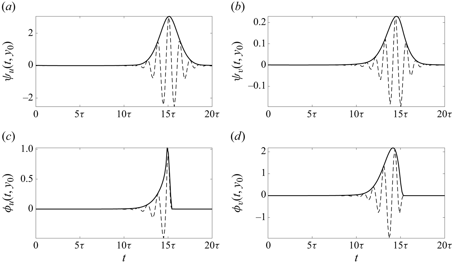
To explore the temporal profiles of the components of these sparse space–time modes, figure 8 shows the cross-sections along the $t$ axis of the sparse modes in figure 7 at the locations in $y$ where the amplitude of the signal finds its maximum. The temporal evolution of the forcing mode components seems to be more localised in these cross-sections, as they abruptly drop to zero near where the amplitude of the response modes finds its maximum value. The locations of the temporal peaks of these mode components is consistent with the discussion above related to figure 7, with the peak amplitude $\phi _v$ preceding that of $\psi _v$, which itself comes prior to the maximum in $\psi _u$. Quantitatively, the time duration between the peaks is of the same order of magnitude as $\tau$, with a time lag of approximately $0.41\tau$ between the peaks in the $v$ components of the forcing and response modes, and a further time lag of $0.68\tau$ between the peak amplitude of the responses in $v$ and $u$. This suggests that the energy transfer between these mode components occurs over a single oscillatory cycle. Note also that the phase lag in between the $\psi _v$ and $\psi _u$ peaks approximately matches the phase difference between the oscillating component of these signals, as both are entirely real near their peak amplitudes. The shape of the streamwise and wall-normal components of the modes (first row in figure 8) displays a Gaussian envelope with a nearly constant phase gradient and a uniform phase variation across all mode components. This could potentially suggest a natural choice of wavelet basis functions for a low-order temporally localised analysis of this flow (Ballouz et al. Reference Ballouz, Lopez-Doriga, Dawson and Bae2023, Reference Ballouz, Lopez-Doriga, Dawson and Bae2024; Madhusudanan & Kerswell Reference Madhusudanan and Kerswell2024). Moreover, the particular shape of the response modes could enable the implementation of wavepacket pseudomode theory to approximate these response modes (Obrist & Schmid Reference Obrist and Schmid2010, Reference Obrist and Schmid2011; Mao & Sherwin Reference Mao and Sherwin2011; Edstrand et al. Reference Edstrand, Schmid, Taira and Cattafesta2018; Dawson & McKeon Reference Dawson and McKeon2019, Reference Dawson and McKeon2020).

Figure 8.

Absolute (solid) and real (dashed) components of the temporal evolution of the sparse modes shown in figures 7(a)–7(d), at the $y$ locations of maximum amplitude ($y_0$).

3.4. Space-time resolvent analysis of a turbulent Stokes boundary layer

In this section we apply non-sparse and sparse space–time resolvent analysis to a turbulent Stokes boundary layer, with a time-periodic mean velocity field as shown in figure 9. This flow sits between two plates that oscillate synchronously with a velocity given by

(3.1)\begin{equation} U_w(t) = U_0\cos{(\varOmega t)}, \end{equation}

with $U_w$ denoting the velocity of the oscillating walls and $U_0$ representing a constant. There is no external pressure gradient, so the flow is entirely driven by the motion of the walls. The Reynolds number for this flow is defined as a function of the frequency of the oscillations $\varOmega$, such that $\textit {Re}_\varOmega =U_0\delta _\varOmega /\nu$, and $\delta _\varOmega =\sqrt {2\nu /\varOmega }$ is a length parameter denoting the boundary layer thickness. For the ensuing analysis, we choose $\textit {Re}_\varOmega =1500$ to ensure that the flow lies in the intermittently turbulent regime (Hino, Sawamoto & Takasu Reference Hino, Sawamoto and Takasu1976; Akhavan, Kamm & Shapiro Reference Akhavan, Kamm and Shapiro1991; Verzicco & Vittori Reference Verzicco and Vittori1996; Vittori & Verzicco Reference Vittori and Verzicco1998; Costamagna, Vittori & Blondeaux Reference Costamagna, Vittori and Blondeaux2003). Note that while there appears to be little prior work performing linear analyses of this configuration in the turbulent regime, linear analysis of laminar pulsatile channel flow has been considered using Floquet analysis (Pier & Schmid Reference Pier and Schmid2017) and optimally time-dependent modes (Kern et al. Reference Kern, Beneitez, Hanifi and Henningson2021).

Figure 9.

(a) Streamwise mean flow $U(y,t)$ (colourmap) and streamwise turbulence intensity $u_{rms}$ (grey dashed) of a turbulent Stokes boundary layer, with levels indicating $\{20\,\%, 30\,\%, 50\,\%, 75\,\%, 95\,\%\}$ of its maximum value, over a full oscillating cycle; (b) time instances of the turbulent mean at $t\varOmega ={\rm \pi}$ (black) and $t\varOmega =3{\rm \pi} /2$ (red).

The mean velocity profile and the root mean square of the fluctuating turbulent velocity components are obtained through DNS as described in § 3.1. The size of the domain for the DNS is $6{\rm \pi} \delta _\varOmega \times 80\delta _\varOmega \times 3{\rm \pi} \delta _\varOmega$ (in the streamwise, wall-normal and spanwise directions, respectively) and contains 64, 385 and 64 grid points in each of the corresponding dimensions. To collect mean data, the DNS was run for 100 eddy turnover times after the decay of transient startup effects, where here we define this time scale as $\delta _\varOmega /u_\tau$, with $\delta _\varOmega =0.025h$. The time-periodic mean velocity profile is obtained through averaging in the dimensions of spatial homogeneity (i.e. the streamwise and spanwise directions) for each phase of wall motion. For resolvent analysis, the size of the numerical domain is $[0,h]\times [0,\tau _{tot}]$ with $h=1$ and $\tau _{tot}$ being the length of the time horizon.

For performing both sparse and non-sparse space–time resolvent analysis, we consider wavelengths corresponding to the extent of the DNS computational domain, i.e. $\lambda _x = 6{\rm \pi} \delta _\varOmega \approx 0.471 h$ and $\lambda _z = 3{\rm \pi} \delta _\varOmega \approx 0.236 h$. That is, we look at the largest three-dimensional structure that the DNS would be capable of resolving. The reason for focusing on such large structures in $x$ and $z$ is that we expect that they will correspond to space–time resolvent modes that also have a large extent in $t$ and $y$, allowing for the distinction between the sparse and non-sparse variants to be clearly observed.

For the non-sparse implementation of resolvent analysis, the domain is discretised using $N_y=105$ collocation points in the wall-normal axis and $N_t=651$ collocation points in the temporal dimension over a time window comprised of one oscillating cycle. The streamwise and wall-normal velocity components of the leading forcing and response modes obtained from this analysis are shown in figure 10, along with the corresponding streamwise and wall-normal turbulence intensity computed from the DNS. Observe that the identified coherent structures do not correspond to a single temporal Fourier mode. Instead, they are concentrated over approximately half of the full oscillation period. Although not shown here, the second leading resolvent mode depicts a coherent structure of almost identical energy content that is similar to the leading modes in figure 10, with a relative temporal shift of a half-period.

Figure 10.

Real component of leading space–time resolvent (a,b) response $\boldsymbol {\psi }_1$ and (c,d) forcing $\boldsymbol {\phi }_1$ modes of the resolvent operator in a turbulent Stokes boundary layer with $\lambda _x/h=0.471$ and $\lambda _z/h=0.236$ during a full oscillating cycle. The grey dashed lines represent the (a,c) streamwise and (b,d) wall-normal turbulence intensity, with contours at $\{15\,\%,20\,\%30\,\%,40\,\%,60\,\%\}$ and $\{22\,\%,30\,\%,45\,\%,55\,\%,70\,\%\}$ of the maximum value of $u_{rms}$ and $v_{rms}$, respectively.

The location of the modes along the $y$ axis shifts away from the wall as the mean flow evolves over time. This angle in the $y\unicode{x2013}t$ plane appears to be similar to that observed for the turbulence intensities, suggesting that the mode depicts an energy transfer mechanism away from the wall that is present in the full nonlinear system. These modes are not concentrated in the near-wall region where the mean shear and turbulence intensity is largest. In this region the turbulent energy content is likely dominated by structures at smaller length scales than the wavelengths considered here. We do observe, however, in figure 10(a) that the streamwise velocity response is amplified as the mode enters a region of higher streamwise turbulence intensity at $(t\varOmega,y/h)\approx ({\rm \pi},0.2)$. In addition, the disturbance streamfunctions identified in Blennerhassett & Bassom (Reference Blennerhassett and Bassom2002) for a flat Stokes boundary layer are similar to the behaviour of the space–time modes presented in figure 10 in two ways: first, the spatial shift of the structures along the wall-normal direction; second, the time-dependent oscillation frequency of these structures. The latter property will be addressed in more depth later in this section.

For the sparse implementation of space–time resolvent analysis at the same wavelengths, we adopt the same time horizon as in the non-sparse case, and a numerical domain with $N_y=101$ collocation points in the wall-normal axis and $N_t=631$ collocation points in the temporal dimension, with a sparsity ratio $\gamma =0.001$ ($\alpha = 0.625$). The location of maximum mode amplitude along the $y$ axis is indicated with a horizontal dotted line, and the value is indicated for each subplot with the symbol with $y_0/h$ and its equivalent in inner units $y_0^+$ for reference.

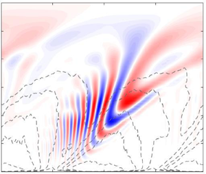
The leading sparse resolvent modes are shown in figure 11, again overlaid with contour levels of the streamwise and wall-normal turbulence intensity. We observe that at these streamwise and spanwise wavelengths, the structure of the leading resolvent modes differs substantially between the non-sparse and sparse analyses. In figure 11 the sparse analysis identifies localised structures for which the streamwise and wall-normal components are concentrated within one quarter of the total temporal domain, and within a small spatial region near $y/h=0.2$ (note that the vertical range shown in figure 11 is smaller than in figure 10). Moreover, both forcing mode components precede their corresponding response modes (shown directly in figure 11e,f), with a peak response in $v$ preceding that for $u$, which was also observed in the sparse modes computed for statistically stationary channel flow in § 3.3. Comparing the sparse modes with the non-sparse counterparts in figure 10, the sparse analysis favours structures that are closer to the peak of the turbulence intensity.

Figure 11.

Real component of sparse space–time leading (a,b) response $\boldsymbol {\psi }_1$ and (c,d) forcing $\boldsymbol {\phi }_1$ modes of the resolvent operator for a turbulent Stokes boundary layer with $\lambda _x/h=0.471$ and $\lambda _z/h=0.236$, computed with a sparsity ratio $\gamma =0.001$, across a full oscillation cycle. Panels (e,f) show contour levels of the absolute value of leading forcing (red) and response (blue) modes. The grey dashed lines represent the corresponding streamwise and wall-normal turbulence intensity, with contour levels at $\{23\,\%,32\,\%40\,\%,50\,\%,70\,\%\}$ and $\{35\,\%,45\,\%,60\,\%,75\,\%\}$ of the maximum value of $u_{rms}$ and $v_{rms}$, respectively. Horizontal dotted lines in (a–d) indicate the $y$ location where each mode component achieves its maximum amplitude ($y_0/h$).

Figure 12 shows cross-sections of these sparse modes along the temporal axis at the $y$ locations where they achieve their maximum amplitude (see the dotted lines indicated in figure 11). Comparing figures 7 and 12, we observe greater variation in the phase both within and across each mode component for the time-varying Stokes boundary layer configuration. For example, the streamwise velocity response in figure 12(a) shows that the rate of phase variation increases over time. The phase variation in the streamwise component of the sparse forcing mode is much slower, which figure 11(c) shows is due to the almost horizontal inclination of this component. As was the case in figure 7, we observe that the forcing mode components have envelopes that are less symmetric in time, abruptly decaying to zero at a given cutoff time.

Figure 12.

Absolute (solid) and real (dashed) components of the temporal evolution of the sparse modes shown in figures 11(a)–11(d), at the $y$ locations of maximum amplitude ($y_0$).

Figure 13 presents the spectral power of the non-sparse (a,b) and sparse (c,d) response modes shown in figures 10 and 11, respectively. Each plot is generated via a temporal Fourier transform at each spatial location along the wall-normal axis ($y$). On the one hand, the regions of higher spectral power corresponding to the sparse modes in figures 13(c) and 13(f) are localised in $y$, but consist of a relatively broad frequency range. Conversely, the regions corresponding to the location of maximum spectral power of the non-sparse modes do not show the same degree of localisation in $y$, and also exhibit several distinct peaks in the ($\omega, y/h$) plane. Furthermore, both the non-sparse and sparse spatio-temporal analyses identify continuous regions of active frequencies. Indeed, the identified modes in figures 10 and 11 depict structures with time-varying frequencies. This evolution of the frequency within a single space–time mode would not be directly captured via harmonic resolvent analysis, where each component mode is associated with a single (discrete) temporal frequency (though triadic interactions between different frequencies could be isolated with this approach). Instead, the superposition of a considerable amount of temporal frequencies would be required to capture the dominant spatio-temporal modes identified by the direct space–time analysis. This suggests that the present approach could be more insightful when applied to flows that do not necessarily possess sparse frequency content, such as the configuration considered in this section.

Figure 13.

Spectral power of the streamwise ($u$) (a,c) and wall-normal ($v$) (b,d) components of the non-sparse (a,b) and sparse (c,d) spatio-temporal resolvent modes presented in figures 10 and 11, respectively. A discrete Fourier transform is computed during one oscillating period at each of the locations of the $y$ axis in the numerical domain.

3.5. Space–time resolvent analysis of a turbulent channel flow with sudden lateral pressure gradient

The last case considered in this work is a fully developed turbulent channel flow at $\textit {Re}_\tau =186$ that is subjected to a sudden lateral pressure gradient at $t=0$. The spanwise pressure gradient is related to the fixed streamwise gradient by $\partial p/\partial z=\varPi (\partial p/\partial x)$, where here we use $\varPi =30$. Additional information about this configuration can be found in Moin et al. (Reference Moin, Shih, Driver and Mansour1990) and Lozano-Durán et al. (Reference Lozano-Durán, Giometto, Park and Moin2020). The turbulent mean flow therefore contains both streamwise $U(y,t)$ and spanwise $W(y,t)$ non-zero components, which evolve over time until the system reaches its new statistically stationary state. These velocity components are shown in figure 14.

Figure 14.

Temporal evolution of the streamwise $U(t,y)$ (black) and spanwise $W(t,y)$ (red) mean velocity profiles obtained by DNS of a turbulent channel flow at $\textit {Re}_\tau =186$ with a sudden lateral pressure gradient at $t=0$ with $\partial p/\partial z=\varPi (\partial p/\partial x)$ and $\varPi =30$ at $tu_\tau /h\in \lbrace 0,0.58,1.17,1.38,1.76,2.34\rbrace$ (Lozano-Durán et al. Reference Lozano-Durán, Giometto, Park and Moin2020).

To form the resolvent operator, the temporal domain is implicitly non-dimensionalised by the initial friction velocity $u_{\tau,0}$ at $t=0$ and $h$, and it is determined in two steps to achieve numerical accuracy. It is first defined as the interval $[-0.58,2.34]h/u_\tau$ to extend the numerical domain before the initial condition to include time prior to the application of the spanwise pressure gradient. Thus, for $t<0$, the base flow is constant, with $U(t<0,y)=U(T=0,y)$ and $W(t<0,y)=0$, and $\partial p/\partial z(t<0)=0$. After a first analysis is conducted, the time domain is restricted to a smaller temporal window near the observed temporal location of the leading modes that is large enough to produce unaltered results with a larger temporal resolution. Note that here we implement an explicit Euler finite-differentiation scheme in the temporal dimension. Thus, the final numerical domain used in this analysis is given by $[0,h]\times [0.4,2]h/u_\tau$.

As was the case for the statistically stationary channel flow studied in §§ 3.2–3.3, we concentrate our analysis on streamwise and spanwise wavenumbers corresponding to the typical size of near-wall streaks. After the pressure gradient is applied, the magnitude and direction of the mean flow changes, meaning that the wavelengths associated with near-wall streaks is also expected to change. Assuming that near-wall streaks adjust their size and orientation with the mean, we can select wavelengths corresponding to the typical size of near-wall streaks at a certain point in time (Ballouz et al. Reference Ballouz, Lopez-Doriga, Dawson and Bae2024) (though as before, we are not guaranteed that the wall-normal location of the resulting modes will match those typical of such streaks). Here, we select $\lambda ^+_x=189$ and $\lambda ^+_z=1890$, which correspond to the typical length of the near-wall streaks at a time instance $t u_\tau /h=1.38$.

For the non-sparse space–time resolvent analysis, the domain is discretised using $N_y=132$ and $N_t=500$ collocation points. The location of the maximum mode amplitude along the $y$ axis is indicated with a horizontal dotted line, and the value is indicated for each subplot with the symbol with $y_0/h$ and its equivalent in inner units $y_0^+$ for reference. Leading resolvent mode components for this analysis are shown in figure 15. We observe that the modes are localised in time, centred near to the nominal time ($t u_\tau /h=1.38$) where the streamwise and spanwise length scales of the modes coincide with near-wall streaks. The structure of the modes share some similarities with those observed for both the non-sparse and sparse analyses of stationary channel flow (figures 5 and 7). In all cases, the wall-normal response consists of vertically aligned structures, while the forcing is inclined upstream in the $y\unicode{x2013}t$ plane. The $u$ component of the response appears to incline further backwards as time progresses in both figures 7(a) and 15(a), though the latter does appear to move towards and move away from the wall as observed in the former. Note that the $u$ component plotted in figure 15 no longer entirely corresponds to the streamwise direction, due to the spanwise pressure gradient.

Figure 15.

Real component of space–time $u$ and $v$ velocity components of the leading (a,b) response $\boldsymbol {\psi }_1$ and (c,d) forcing $\boldsymbol {\phi }_1$ modes of the space–time resolvent operator for a channel flow with a sudden lateral pressure gradient with $\textit {Re}_\tau =186$, and $\lambda ^+_x=189$, $\lambda ^+_z =1890$. (e,f) Contour levels of the absolute value of the leading forcing (red) and response (blue) modes. Horizontal dotted lines in (a–d) indicate the $y$ location where each mode component achieves its maximum amplitude ($y_0/h$). The grey dashed lines represent the boundaries of the temporal numerical domain.

Figures 15(e)–15(f) show that the forcing and response mode components are all located over approximately the same time interval for this case. This is different from the sparse analysis of statistically stationary channel flow (see figure 7e,f), where the forcing mode components decayed before their responses did, and the wall-normal forcing and response components started before the streamwise components. These differences can likely be attributed to the differences in how localised modes are obtained; for the three-dimensional channel configuration we are not explicitly promoting sparse modes, but rather the modes are aligning with a region of time corresponding to a mean flow with maximum linear energy amplification for structures at the specified spatial scales. This can be further explored by applying the sparse variant to this configuration.

For the sparse implementation of space–time resolvent analysis, we adopt the same wavelengths and a sparsity ratio $\gamma =0.001$ ($\alpha = 0.781$). The domain is discretised using $N_y=130$ and $N_t=500$ collocation points. The leading sparse modes are shown in figure 16, where both the $u$ and $v$ components display a similar structure, but with more temporal localisation, to those shown for the non-sparse analysis in figure 15. The location of the maximum mode amplitude along the $y$ axis is indicated with a horizontal dotted line, and the value is indicated for each subplot with the symbol with $y_0/h$ and its equivalent in inner units $y_0^+$ for reference.

Figure 16.

Real component of sparse space–time $u$ and $v$ velocity components of the leading (a,b) response $\boldsymbol {\psi }_1$ and (c,d) forcing $\boldsymbol {\phi }_1$ modes of the space–time resolvent for a channel flow with a sudden lateral pressure gradient with $\textit {Re}_\tau =186$, and $\lambda ^+_x=189$, $\lambda ^+_z =1890$ with a sparsity ratio $\gamma =0.001$ ($\alpha = 0.781$). (e,f) Contour levels of the absolute value of the leading forcing (red) and response (blue) modes. Horizontal dotted lines in (a–d) indicate the $y$ location where each mode component achieves its maximum amplitude ($y_0/h$). The grey dashed lines represent the boundaries of the temporal numerical domain.

The sparse analysis thus appears to identify the same mechanism, localised around the same region in time. Unlike the non-sparse version, here we observe in figures 16(e)–16(f) differences in the temporal footprints of each mode component, with the decay in amplitude of both components of the forcing preceding the decay of the response.

The cross-sections along the time axis of the modes contained in figures 15 and 16 are shown in figure 17 in red and black, respectively. The amplitudes of both the non-sparse and sparse modes adopt qualitatively similar envelopes, with the sparse variant being narrower, and centred at a slightly later time. We emphasise that unlike the profiles shown in figure 8, here the time location of these modes is not arbitrary and corresponds to a region of time where the mean profile enables the largest linear amplification. The phase variation is similar across all mode components, indicating a characteristic frequency maximising amplification. Here, we thus find that both sparse and non-sparse space–time resolvent analyses appear to identify the same amplification mechanism, with the addition of the $l_1$-norm term in the objective function restricting the sparse modes to a smaller temporal window.

Figure 17.

Absolute (solid) and real (dashed) components of the temporal evolution of the non-sparse modes shown in figures 15(a)–15(d) (red) and sparse modes shown in figures 16(a)–16(d) (black), at the $y$ locations of maximum amplitude.

Lastly, to demonstrate the numerical convergence of the results presented in this section, figure 18 presents the first 10 singular values of the non-sparse and sparse space–time resolvent operators with $\gamma \in \lbrace 0.001,0.15 \rbrace$ space–time resolvent operators against the leading singular values obtained in the study described in Ballouz et al. (Reference Ballouz, Lopez-Doriga, Dawson and Bae2024), where the numerical methods utilize a wavelet transform in time. The corresponding leading modes coincide with figure 15 and figure 16 in the non-sparse and sparse with $\gamma = 0.001$ ($\alpha = 0.781$) implementation of the space–time analysis, respectively. First, observe that the singular values of the non-sparse analysis closely match the reference values. Second, a sparsity ratio of $\gamma =0.15$ ($\alpha = 0.004$) is sufficiently large to obtain similar amplification levels to these reference values (note that the corresponding modes are not shown in this paper). This agreement also confirms the convergence of the sparse analysis. However, the singular values retrieved from the sparse analysis with $\gamma = 0.001$ ($\alpha = 0.781$) and $\gamma = 0.005$ ($\alpha = 0.258$) retrieve only a portion of the reference values. In particular, the leading reference value is larger than the leading sparse singular value with $\gamma = 0.001$ by a factor of 2.0958, and we observe that this ratio decreases for higher-order singular values. The fact that the sparse and non-sparse analyses yield similar results for this case is likely due to the highly transient nature of the flow, where the leading resolvent modes are naturally localised even without explicitly promoting sparsity.

Figure 18.

Leading $10$ singular values of the non-sparse and sparse (with $\gamma \in \lbrace 0.001,0.15 \rbrace$) space–time resolvent operator for a channel flow with a sudden lateral pressure gradient with $\textit {Re}_\tau =186$, and $\lambda ^+_x=189$, $\lambda ^+_z =1890$. The reference values correspond to the analysis described in Ballouz et al. (Reference Ballouz, Lopez-Doriga, Dawson and Bae2024).