



1. Introduction
There are numerous (well in excess of 100) computational and experimental studies, many reviewed in Choi (Reference Choi2000), Karniadakis & Choi (Reference Karniadakis and Choi2003), Quadrio (Reference Quadrio2011), Abdulbari et al. (Reference Abdulbari, Yunus, Abdurahman and Charles2013), Asidin et al. (Reference Asidin, Suali, Jusnukin and Lahin2019), Zhang, Shan & Xie (Reference Zhang, Shan and Xie2020), Leschziner (Reference Leschziner2020) and Ricco, Skote & Leschziner (Reference Ricco, Skote and Leschziner2021), which demonstrate that the imposition of periodic and/or spatially varying spanwise wall motion onto streamwise-oriented near-wall flows in channels, on single walls and in pipes results in a substantial reduction in turbulent drag. A similar response arises from analogous spanwise body forcing within the viscous sublayer (e.g. Yao et al. Reference Yao, Chen, Thomas and Hussain2017; Du & Karniadakis Reference Du and Karniadakis2000) or from plasma-induced unsteady transverse motion (e.g. Choi, Jukes & Whalley Reference Choi, Jukes and Whalley2011; Wong et al. Reference Wong, Zhou, Li and Li2015; Corke & Thomas Reference Corke and Thomas2020). Although the level of the drag reduction depends sensitively on the actuation parameters – the spanwise wall-motion amplitude, the actuation period and/or the wavelength of the spatially varying motion, in particular – the gross and net drag-reduction margins can reach approximately 45 % and 20 %, respectively, in the most favourable scenario in which the oscillatory spanwise wall motion is imposed in the form of streamwise waves in channel flow at a friction Reynolds number  $Re_{\tau } = 250$ (Quadrio, Ricco & Viotti Reference Quadrio, Ricco and Viotti2009).
Aside from the obvious challenges of realising the potential of the above-mentioned control methods in a practical environment, one potentially serious obstacle is that the drag-reduction margin declines with increasing Reynolds number. Extensive simulation studies in channel flow at friction Reynolds numbers up to  $Re_\tau = 1600$ (Hurst, Yang & Chung Reference Hurst, Yang and Chung2014), 2000 (Gatti & Quadrio Reference Gatti and Quadrio2013) and 2100 (Yao, Chen & Hussain Reference Yao, Chen and Hussain2018), suggest a decline in drag reduction in proportion to
 $Re_\tau ^\alpha$, the exponent
 $\alpha$ being in the range 0.1–0.46, depending strongly on the actuation scenario, with additional uncertainties arising from drastic differences in the computational boxes. Alternatively, Gatti & Quadrio (Reference Gatti and Quadrio2016) suggest that, for judiciously chosen actuation parameters, and provided the log-law slope is invariant in all circumstances, the decline in drag-reduction effectiveness can be depressed to the slower logarithmic variation
 \begin{equation} \sqrt{\frac{2}{C_{f}}}-\sqrt{\frac{2}{C_{f, 0}}}=\frac{1}{\kappa} \ln \left(\frac{R e_{\tau}}{R e_{\tau, 0}}\right)+{\rm \Delta} B^{+}, \end{equation}
in which  $C_f$ and
 $C_{f,0}$ are the friction factors of the actuated and the unactuated flow, respectively, and
 ${\rm \Delta} B^+$ is the upward shift in the log law, which is held to depend solely on the drag-reduction margin and
 $C_{f,0}$. As
 ${\rm \Delta} B^+$ is observed, within the modest range for which direct numerical simulation (DNS) data are available, to approach a constant value as the bulk Reynolds number,
 $Re_b$, increases, the implication is that the sensitivity of the drag-reduction margin on the Reynolds number is governed only by the functional dependence
 $C_{f,0}(Re_b)$.
Whether or not the assumptions underpinning (1.1) are valid, it is an inescapable fact that the processes that play a role in the decline of the drag-reduction margin are unclear, especially at more than a modest Reynolds-number range, and this ambiguity is part and parcel of a much wider debate, punctuated by many conflicting paradigms (e.g. Ricco et al. Reference Ricco, Ottonelli, Hasegawa and Quadrio2012; Agostini, Touber & Leschziner Reference Agostini, Touber and Leschziner2015), purporting to explain the physical interactions that are responsible for the drag reduction and its complex dependence on the actuation parameters.
One important element in the mix of arguments is that the actuation-induced directional rate of change in the strain rate within the viscous sublayer disrupts the processes that are responsible for the formation and sustenance of the streaks and quasi-streamwise vortices, reflecting the lift-up, bursting and regeneration mechanisms. A remarkable observation at nearly optimal actuation parameters, for which the drag-reduction margin is maximised, is that the streaks are severely damped during portions of the (sinusoidal) actuation cycle in which the strain vector in the viscous sublayer rotates at a rapid rate, while the streaks tend to strengthen at portions in which the strain rate changes slowly, i.e. when the strain ‘lingers’. If the time scale of the actuation is comparable to, or shorter than, the streak regeneration time scale, the streaks remain weak and the drag, once reduced, fails to recover.
As the Reynolds number increases, there is an increasing tendency of the broadening spectrum of turbulent structures in the log-law region to impact the viscous sublayer. While this intensification does not express itself by major changes to the universal behaviour of inner-scaled properties of the canonical flow close to the wall, the effectiveness of the oscillatory spanwise forcing diminishes, at least in line with (1.1), as the viscous sublayer is progressively more ‘agitated’ by footprinting of the turbulent motions. However, a potentially influential additional mechanism that emerges with increasing Reynolds number, over and above those in the universal near-wall layer, is a distinctive Reynolds-number-dependent elevation of the streamwise turbulence intensity around the location  $y^+=\frac{y u_{\tau}}{\nu} \approx 4 \sqrt{Re_{\tau}}$, as proposed by Mathis, Hutchins & Marusic (Reference Mathis, Hutchins and Marusic2009), based on experimental data for boundary layers at
 $Re_\tau$ up to
 $19\ 000$. This elevation gives rise to a near-horizontal plateau in a planar boundary layer at sufficiently high Reynolds number (Örlü et al. Reference Örlü, Fiorini, Segalini, Bellani, Talamelli and Alfredsson2017), or a ‘second maximum’ in pipe flow (Smits, McKeon & Marusic Reference Smits, McKeon and Marusic2011), the ‘first maximum’ being at
 $y^+\approx 12.5$. The elevation in intensity reflects the presence of large-scale ‘super-streaks’ that appear to be sustained, as will be shown by the results to follow, by large-scale sweeps and ejections similar to those giving rise to the streaks in the buffer layer. In channel flow, the statistical dimensions of these structures scale with the channel half-height, their length being of order 5–10 half-heights long and being separated by approximately 0.5 half-height (Del Álamo & Jiménez Reference Del Álamo and Jiménez2003; Hoyas & Jiménez Reference Hoyas and Jiménez2006; Agostini & Leschziner Reference Agostini and Leschziner2017).
A substantial body of work that has exposed and quantified the effects of the outer high-energy layer on the near-wall region of canonical boundary layers has been published by Marusic and collaborators (Marusic & Heuer Reference Marusic and Heuer2007; Hutchins et al. Reference Hutchins, Nickels, Marusic and Chong2009; Marusic, Mathis & Hutchins Reference Marusic, Mathis and Hutchins2010). These studies, reporting statistical data derived from hot-wire anemometry (HWA) measurements, identify large-scale ‘footprinting’ in the viscous sublayer, closely correlated with the outer structures, and the ‘modulation’ (amplification and attenuation) of small-scale motions within large-scale footprints as being the primary effects of the outer structures on the viscous sublayer. Agostini & Leschziner have subsequently reported several studies (Agostini & Leschziner Reference Agostini and Leschziner2014, Reference Agostini and Leschziner2016; Agostini et al. Reference Agostini, Leschziner, Poggie, Bisek and Gaitonde2017; Agostini & Leschziner Reference Agostini and Leschziner2018) in which DNS data for canonical channel flow were analysed to reveal structural aspects as well as statistical manifestations of footprinting and modulation, in addition to which ‘splatting’ by large-scale sweeps was identified as provoking a substantial asymmetry and hysteresis in the response of the near-wall properties to the outer large scales. Their analysis hinged on the application of the empirical mode decomposition (EMD), outlined in § 3 below, to separate large from small scales in hundreds of full-volume DNS realisations, allowing small-scale statistics conditional on spatial sub-volumes of large-scale motions to be derived. The only application of the EMD to actuated channel flow using the above methodology is that of Agostini & Leschziner (Reference Agostini and Leschziner2018), in which the asymmetric effect of the outer structures was investigated for streamwise-homogeneous oscillatory wall motion at  $T^+=T{u_\tau }^2/\nu =100$ and
 $200$.
An illustration of the processes that are the focus on the influence of outer structures is given in figure 1, which arises from DNS data for a channel flow subjected to oscillatory wall motion at  $T^+=100$ (Agostini, Touber & Leschziner Reference Agostini, Touber and Leschziner2014). This shows wall-parallel fields of streamwise-velocity fluctuations at an identical time level, figure 1(a) being for
 $y^+\approx 200$, figure 1(b) being for
 $y^+\approx 18$ and figure 1(c) for
 $y^+\approx 3$, the latter effectively representing the skin friction. The choice
 $y^+\approx 200$ is based on the observation that this location lies within the region of elevated streamwise energy, reflecting the presence of the large-scale structures of primary interest herein. The pattern shown in figure 1(a) suggests the presence of large, coherent, streaky structures with a length scale of order
 $5h$, where h is the channel half-height, separated by a distance of order
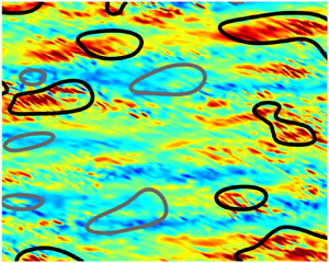
 $1h$. More pertinent to the present argument is the fact that the field in figure 1(c) shows clear footprints that are closely correlated with the outer structures, thus implying that the processes in the forced near-wall layer be sensitive to the outer structures. Closer inspection of the red regions of positive fluctuations reveals the presence of fine inclined streaks which are associated with the lift-up mechanism within the viscous and buffer regions, the inclination being due to the spanwise Stokes strain that is induced by the wall motion. The streaks are separated by roughly 100 wall units in the spanwise direction (as will be seen more clearly in figure 3). No streaks are visible within the negative large-scale footprints. This qualitative difference is rooted in the modulation of the small near-wall scales by the footprints: positive footprints amplify small-scale fluctuations, while negative footprints tend to attenuate these fluctuations. A detailed discussion of the physical response of the streaks to the spanwise strain is given in Touber & Leschziner (Reference Touber and Leschziner2012).
Streamwise-velocity fluctuations across three wall-parallel planes in channel flow at  $Re_\tau \approx 1025$ with oscillatory spanwise motion at
 $T^+=100$: (a)
 $y^+\approx 200$, (b)
 $y^+\approx 18$ and (c)
 $y^+\approx 3$. The colour scales indicate wall-scaled velocity.

The above reference to ‘negative large-scale footprints’ requires a terminological qualification. A strict interpretation of footprinting is that this process is associated only with positive large-scale near-wall fluctuations, which are induced by sweeping motions. However, irrespective of formal causation arguments (Lozano-Durán, Bae & Encinar Reference Lozano-Durán, Bae and Encinar2020), positive and negative large-scale events are intimately linked, via the association of sweeps with ejections, the latter linking events near the wall to those in the outer region. Thus, footprints arguably encompass both positive and negative large-scale fluctuations induced by the outer-flow motions. This is a justification for ‘negative footprints’ and large-scale negative fluctuations being used synonymously in the present paper.
Apart from illuminating the decline and amplification in streak strength within positive and negative large-scale footprints, respectively – and hence corresponding reduction and increase in local friction drag – the analysis brought to the fore a strong asymmetry in the footprinting, with positive large-scale footprints being much more intense than negative ones, a process associated with ‘splatting’. In Agostini & Leschziner (Reference Agostini and Leschziner2014), the EMD methodology was then extended to allow the analysis of an actuated channel flow at  $Re_\tau \approx 1025$ subjected to streamwise-homogeneous oscillatory wall motion at
 $T^+=100$ and 200. The results provided further evidence for the disproportionate impact of positive footprints on the near-wall statistics, including the streamwise intensity and the shear stress, sampled conditionally on large-scale skin-friction fluctuations. This was thus interpreted as providing evidence for the increasing damage that large-scale footprints cause to the drag-reduction effectiveness as the Reynolds number increases. One other important result derived from the EMD methodology was that the large-scale motions were responsible, on their own – i.e. without their effects on the small-scale processes – for approximately 25 % of the total skin friction.
A limitation of the methodology used in Agostini et al. (Reference Agostini, Touber and Leschziner2014, Reference Agostini, Touber and Leschziner2015) is that it did not allow the mechanisms and interactions responsible for the asymmetric impact described above to be identified. This limitation was addressed by Agostini & Leschziner (Reference Agostini and Leschziner2019a) through the extraction from DNS data for unactuated channel flow of multi-dimensional probability-density functions (PDFs) of the form  $P(X_1,\ldots ,X_i,\ldots ,X_N, Cf_{LS})$, where
 $X_i$ is the turbulent fluctuation of any flow variable and
 $Cf_{LS}$ are large-scale skin-friction fluctuations, derived from the EMD. This then allowed a variety of conditional statistical properties to be derived, including turbulent-production levels, allowing the processes driving the total, large-scale and small-scale stresses to be studied. The present study applies this novel methodology to channel flow subjected to oscillatory spanwise motion at
 $T^+=100$. The principal purpose of doing so is to investigate whether the oscillatory wall motion leads to a fundamental change in the response of the near-wall small scales to the outer large scales, this mechanism being specifically pertinent to the drag-reduction effectiveness of the actuation.
2. The configuration examined
The analysis previously described is performed on DNS data for a streamwise and spanwise periodic channel flow at friction Reynolds number  $Re_\tau \approx 1025$, having a half-height
 $h$ and dimensions
 $6{\rm \pi} h \times 2{\rm \pi} h \times 2h$ covered with a mesh of 500 million cells. The upper and lower walls are actuated in phase with the streamwise-homogeneous spanwise velocity
 \begin{equation} W(t)=W_m^+ \sin(2{\rm \pi} t/T^+), \end{equation}
where  $W_m^+=W_m/u_\tau =12$ and
 $T^+=100$, the latter value giving rise to the highest drag-reduction margin, at 30 %, achievable with a streamwise homogeneous actuation. The details of the simulation are comprehensively covered in Touber & Leschziner (Reference Touber and Leschziner2012) and Agostini et al. (Reference Agostini, Touber and Leschziner2014). It is important to make clear here that the 30 % reduction in drag results in a reduction in
 $Re_\tau$ from 1025 to 875, while the bulk Reynolds number is maintained at the same level. In the presentation of results to follow, wall scaling is effected, unless otherwise stated, with the
 $u_\tau$ value of the actuated case. Because of the reduced value of
 $Re_\tau$, the intensity of the energetic outer structure that plays a central role in the present study is somewhat weaker than that in the canonical (unactuated) case considered in Agostini & Leschziner (Reference Agostini and Leschziner2019a), and so are the interactions that are discussed herein.
A total of 500 full-volume realisation have been collected over a period  $t^+=5000$, corresponding to 50 actuation cycles. At the present actuation period, the flow conditions are virtually unaffected by the periodicity of the actuation – i.e. the drag shows insignificant oscillations around the low-drag level of 70 % of the unactuated case. Hence, the temporal or phase location of any of the 500 realisations relative to the actuation cycle is of no importance.
3. Statistical processing
To examine the scale interactions of interest, the velocity field is decomposed into wavelength modes by means of EMD Huang et al. (Reference Huang, Shen, Long, Wu, Shih, Zheng, Yen, Tung and Liu1998). The method originates from the signal-processing domain, and has conventionally been used to decompose one-dimensional (1-D) spatial or temporal functions into modes, each of which comprises a narrow range of time or length scales. In the present 3-D context, the method has been generalised to the decomposition of any spatial-variable field  $f(x,z)$ across any wall-parallel
 $(x,z)$ plane at a wall distance
 $y$. The EMD thus represents the field by a set of ‘intrinsic mode functions’ (imfs) and a residual:
 \begin{equation} f(x, z)|_{y}=\sum_{n=1}^{m} imf_{n}(x, z)+R(x, z). \end{equation}
The process starts by constructing envelopes of the minima and maxima of the signal, yielding the surfaces  $E_{high}(x,z)$ and
 $E_{low}(x,z)$, respectively. The mean of the two envelopes is then computed as
 $E_{mn}(x,z) = (E_{high}(x,z) + E_{low}(x,z))/2$. This mean is then subtracted from
 $f(x,z)$ to yield a residual
 $R(x,z)=f(x,z)-E_{mn}(x,z)$. This residual constitutes the first approximation of
 $imf_1$. The above process, referred to as ‘sifting’, is repeat, using
 $f(x,z)\leftarrow f(x,z)-R(x,z)$ as the input field, until a pre-defined stopping criterion is reached. The residual is then deemed to have converged to the first imf,
 ${R(x,z)=imf_1(x,z)}$. The above process is repeated on the field
 $f(x,z)\leftarrow f(x,z)-imf_1(x,z)$ to yield subsequent modes,
 $imf_i$, the end result being
 $m$ imfs plus the residual. All
 $y$-planes are treated sequentially in an analogous manner.
In the present application, mode  $imf_1$ corresponds to the smallest-scale motions associated with the streaks in the buffer layer, while subsequent modes capture sub-ranges of increasing length scale. A property of the EMD is that a mode
 $imf_i$ has a mean length scale that is twice the previous one,
 $imf_{i-1}$. It follows that a continuation of the decomposition eventually ends when the modes have negligible energy. The number of pertinent modes is therefore dependent on the range of length scales of the signal – i.e. the Reynolds number of the flow being considered.
In contrast to other methods, e.g. proper orthogonal decomposition (POD), the EMD requires no pre-determined functional elements, such as Fourier or wavelet functions. Rather, the imfs are the data-driven basis functions generated by the EMD, which arise purely from the baseline signal itself. The method does not imply linearity, involves no frequency or length-scale cutoffs and is energy conserving.
The above decomposition is exemplified by figure 2(a), which shows the spanwise spectrum of streamwise-velocity fluctuations for the present actuated channel flow. The colour contours indicate the five modes arising from the decomposition, the residual on the extreme right-hand side being omitted. Modes 1 and 2 are deemed to be ‘small’, while modes 4 and 5 are regarded as ‘large’, the two being separated by the ‘intermediate’ mode 3. Importantly, the sum of the contributions of the scales to any energy component or the shear stress, including components that represent interactions between scales, is identical to the relevant total stress derived directly from the DNS. This is illustrated in figure 2(b), which shows profiles of scale-wise contributions to the streamwise stress, except from a minor scale-interaction component. The profiles demonstrate that the large-scale component persists across the entire near-wall layer, penetrating well into the viscous sublayer, thus representative of footprinting. In the buffer layer,  $y^+ \approx 20$ (rather than 12–15 in the unactuated flow), where the streamwise stress reaches its maximum, the small-scale component dominates. This behaviour is in accord with expectation, as the buffer region is where the small-scale streaks are most pronounced.
Contribution of different scales to streamwise turbulence energy in channel flow at  $Re_\tau \approx 1025$ and
 $T^+=100$; (a) premultiplied spanwise spectral map; grey contours represent the total field; coloured iso-lines represent sub-spectra for the different EMD modes and the residual; (b) scale-wise contributions to streamwise energy: blue line represent small scales (modes 1 and 2,
 $\overline {u_{SS}u_{SS}}^+$), red line represents large scales (mode 4, mode 5 and residual,
 $\overline {u_{LS}u_{LS}}^+$), green line represents intermediate scales (mode 3), black line is the total stress (
 $\overline {u^{\prime } u^{\prime }}^+$).

With the decomposition achieved, the effects of the large-scale motions on the properties of the flow as a whole or its small-scale components can be studied. One outcome of the application of the EMD is the PDF of the large-scale skin-friction fluctuations, shown in figure 3(a). This PDF arises from the assumption that the large-scale motion is captures by right-most modes 4 and 5 in figure 2(a) and residual. These structures are seen to cover the spanwise scale within the approximate range  $\lambda _z^+ =800 - 2000$ - i.e.
 $0.8 - 2h$ (as shown in figure 1a). They originate at
 $y^+ \approx 200$ and persist across almost the entire layer below this position by virtue of the footprinting mechanism.
Illustration of EMD processing across one wall-parallel plane at  $y^+\approx 3$; (a) PDF of large-scale streamwise-velocity fluctuations derived from EMD, dashed dark blue and red lines correspond to
 $1\,\%$ extreme events, light blue and orange lines correspond to
 $10\,\%$ and green line to
 $50\,\%$ (median of PDF); (b) large-scale fluctuations obtained by summing up all EMD modes (4 and above) across one quarter of the computational box; (c) full field of streamwise fluctuations: black and grey iso-lines correspond to the
 $15\,\%$ extreme large-scale positive and negative large-scale fluctuations, respectively. Inclined small-scale streaks within black islands reflect the influence of the spanwise Stokes layer.

The PDF of the large-scale skin-friction fluctuations (figure 3a) is seen to be highly asymmetric. figure 3(c) shows a snapshot of the raw turbulent fluctuation field at  $y^+=3$, which is effectively a surrogate of the skin friction. Attention is drawn to the fact that the plots cover one quarter of the extent of the wall-parallel computational domain. An interesting feature to highlight here is the pronounced skewed small-scale patterns within the high-speed red regions. These are the near-wall streaks, tilted by the Stokes strain. When the EMD is applied to this field, the large-scale fluctuations can be isolated, and these are shown in figure 3(b). The islands identify the extreme
 $+$15 % and
 $-$15 % large-scale fluctuation events within the tails of the PDF of the large-scale motions on this plane. In the methodology reported in Agostini, Leschziner & Gaitonde (Reference Agostini, Leschziner and Gaitonde2016) and Agostini & Leschziner (Reference Agostini and Leschziner2018), the turbulence statistics – e.g. small-scale stresses – conditional on the large-scale motions were determined by sampling the small-scale motions within islands of the type shown in figures 3(b) and 3(c). More precisely, the large-scale PDF was divided into 5 % bins, and sampling was done within these bins at all
 $y^+$ planes for which DNS data were available.
4. The joint-probability-density function analysis
In a recent paper (Agostini & Leschziner Reference Agostini and Leschziner2019a,Reference Agostini and Leschzinerb), a novel, more general approach to analysing any statistical flow property conditional on any value of the large-scale skin-friction fluctuation was presented and applied to canonical (unactuated) channel flow. The principal merit of the approach is that it allows a transparent identification of the mechanisms responsible for the observed response of the turbulent statistics to the large-scale motions. Here, only its key elements are summarised.
The general joint PDF  $P(X_1,\ldots ,X_n,Y)$, in which
 $Y$ identifies a ‘conditional variable’, is considered. Here,
 $X$ can be any turbulent flow property or a property specific to a spectral sub-range within the spectrum shown in figure 2(a).
The following properties can be then examined:
 $$\begin{gather} \frac{\textrm{d} \overline{X_i}}{\textrm{d} Y} =\int_{- \infty }^{+\infty} \cdots \int_{- \infty }^{+\infty} X_i P(X_1,\ldots,X_n,Y) \, \textrm{d} X_1 \ldots\, \textrm{d} X_n, \end{gather}$$
 $$\begin{gather}\frac{\textrm{d} \overline{x_i^{\prime} x_j^{\prime}}}{\textrm{d} Y} = \frac{\textrm{d} \overline{X_iX_j}}{\textrm{d} Y}- \frac{\textrm{d} \overline{X_i}}{\textrm{d} Y} \frac{\textrm{d} \overline{X_j}}{\textrm{d} Y}. \end{gather}$$
These derivatives represent the contribution of the properties in question to their respective totals within a band of  $dY$, and their integral with respect to
 $Y$ then yields the property itself.
A second set of informative statistical quantities are the conditional mean values and associated variances
 \begin{equation} \overline{X_i}|_{Y}=\int_{- \infty }^{+\infty} \cdots \int_{- \infty }^{+\infty} X_i \frac{P(X_1,\ldots,X_n,Y)}{P(Y)}\, \textrm{d} X_1 \cdots\, \textrm{d} X_n,\end{equation}
 \begin{align} \overline{x_i^{\prime} x_j^{\prime} }|_{Y} &= \overline{(X_i-\overline{X_i}|_Y) (X_j-\overline{X_j}|_Y)} |_Y \nonumber\\ &=\overline{X_i X_j}|_Y - \overline{X_i}|_Y \overline{X_j}|_Y. \end{align}
The merit of these conditional values for the mean and the variance is that they bring to light the influence of large-scale fluctuations on the quantities considered at large positive and negative  $Y$ values without the obscuring influence, or weighting, of the low density levels in the PDF
 $P(Y)$.
In the particular application pursued herein,  $X_i$ are instantaneous velocity components, while
 $Y$ is the local and instantaneous skin friction that is driven by the large-scale footprints,
 $Cf_{LS}$. In other words, the variation of statistical properties of the turbulent velocity field – e.g. stresses and their production rates – as a function of
 $Cf_{LS}$ is examined, allowing the contribution of the pertinent statistical properties to be related to the sign and magnitude of the large-scale skin-friction footprints. As the actuated channel flow is statistically streamwise homogeneous, the statistical properties only depend on the wall distance
 $y$, so that any statistical property can be conveyed by contour maps in the
 $y - Cf_{LS}$ plane, the lag between wall fluctuations and the rest of the flow being removed.
5. Results
5.1. Mean flow
The dependence of the mean-flow properties on the intensity of the large-scale footprints is conveyed in figure 4. An important reason for examining these properties, in particular the strain rate, is that they are relevant, in conjunction with the Reynolds stresses, to the stress-production levels and also to the response of the small-scale turbulence levels near the wall to the footprints.
Velocity and strain fields conditional on large-scale skin-friction fluctuations: (a) mean streamwise-velocity field relative to the average ( $\overline {u}^+|_{Cf_{LS}} -\overline {u}^+$); (b) velocity profiles at the five locations marked in the PDF in figure 3(a); (c,d): as (a,b), respectively, but for the wall-normal velocity; (e,f) as (a,b), respectively, but for the streamwise shear strain rate (
 $\textrm {d} \overline {u}^+|_{Cf_{LS}}/{\textrm {d} y}-\textrm {d} \overline {u}^+ / {\textrm {d} y}$). Dashed lines in (b,d, f) are the respective mean profiles. Grey line and curve in (b) represent the canonical log law and viscous-layer profile, respectively. Grey curve in (a,e is the locus
 $y^+_{LS}\approx 12$, with
 $LS$ denoting scaling with large-scale friction velocity.

Figures 4(a), 4(c) and 4(e) show, respectively, maps of the streamwise velocity, wall-normal velocity and strain rate, all three conditional on the large-scale skin-friction fluctuations  $Cf_{LS}$. These maps arise from the application of the normalised PDFs, (4.3), the aim being to avoid the obscuring influence of low probability density within the tails of the PDF in figure 3(a), and they thus bring out the impact of the large-scale footprints relative to number of
 $Cf_{LS}$ events (or probability density). The five full-line profiles in figures 4(b), 4(d) and 4(f) are sections through the corresponding contour maps at the five locations marked in figure 3(a), the two locations on either side of the PDF median value bounding 10 % and 1 % of the extreme events, respectively. In addition, the dashed-line profiles represent the respective mean values across the entire
 $Cf_{LS}$ range, the grey curve in figure 4(a) is the locus of
 $y^+_{LS}=12$, in which
 $LS$ identifies scaling with the large-scale friction velocity, and the grey lines in figure 4(b) identify the canonical log law and the viscous-layer law, respectively. As regards the last item, attention is drawn to the fact that the mean-velocity profiles lying above the canonical log law is a well-known manifestation of the reduced drag level resulting from the actuation. The discontinuities in the slope of some of the profiles and contours in the outer region are due to the fact that the unsteady-flow data arising from the DNS were only saved at a relatively small number of wall-normal planes beyond
 $y^+ \approx 80$.
The results in figure 4 reveal six features that deserve to be brought out:
• The velocity and strain fields respond asymmetrically to
 $Cf_{LS}$, and so do the thicknesses of the viscous sublayer, in consonance with the asymmetric PDF shown in figure 3(a).
• As the
$Cf_{LS}$ fluctuations increase, in the positive range, the velocity increases across the entire near-wall layer, but especially steeply around the buffer layer. Conversely, the velocity decreases throughout the layer for negative $Cf_{LS}$ fluctuations, and again, especially around the buffer layer, as is indicated by the grey line in figure 4(a), which characterises the response of the viscous sublayer to the footprints. The fact that this line passes through the minimum and maximum contour values has no obvious physical relevance – except insofar as the wall-normal locations of the maximum increase in the streamwise velocity at positive $Cf_{LS}$ values and its maximum decrease at negative $Cf_{LS}$ values, as well as the variations in the thickness of the viscous sublayer and the location of maximum velocity curvature, are all driven in the same direction by the action of the conditional wall-normal motions shown in figures 4(c) and 4(d).• Associated with the increase and decrease in the streamwise velocity are, respectively, large-scale downward and upward motions – i.e. large-scale sweeps and ejections – the latter being more intense than the former at the extreme levels of the large-scale footprints.
• For positive
$Cf_{LS}$ fluctuations, the strain increases steeply in the viscous sublayer, and decreases above $y^+ \approx 12$.• For negative
$Cf_{LS}$ fluctuations, there is an increase in the strain, albeit weak, in the outer layer $y^+ \approx 30 - 90$.• For negative
$Cf_{LS}$ fluctuations, the strain decreases in the viscous sublayer, but at a magnitude much lower than the increase for positive $Cf_{LS}$ fluctuations. At the largest positive value of $Cf_{LS}$, the location of maximum curvature (the gradient of the strain profiles) moves markedly towards the wall, and this is consonant with the thinning of the viscous sublayer, as indicated by the grey line in figure 4(a).


The fact that the impact of the outer large scales on the strain in the buffer layer is rather weak might suggest that the distortions provoked by the large scales may not result in changes to the turbulent state in the buffer layer, the region in which the streaks reside and which is important to the drag. However, as will emerge below, in the examination of the strain-driven production rate, there is a strong increase in the shear stress in the buffer layer, for positive footprints, due to increased production rates of both the streamwise and shear stress, and hence an amplification of the streaks, associated with increased drag.
5.2. Stress fields
Figures 5(a) and 5(c) show maps of the  $Cf_{LS}$-wise rate of change of the streamwise stress
 $(\textrm {d} \overline {u^{\prime } u^{\prime } }^+(y^+)/\textrm {d} Cf_{LS})$ and the shear stress
 $(-\textrm {d} \overline {u^{\prime } v^{\prime }}^+(y^+)/\textrm {d} Cf_{LS})$, derived from 4.2. These allow an appreciation to be gained of how the stresses increase across the range of
 $Cf_{LS}$ and how this increase varies across the boundary layer. The black profiles on the right-hand side arise upon integrating the corresponding left-hand side maps across the
 $Cf_{LS}$ range and represent the actual statistical averages of the stresses across the boundary layer. The solid red and blue profiles represent, respectively, partially integrated stress levels over the segments to the right and left of the median of the
 $Cf_{LS}$ PDF in figure 3(a) – i.e. essentially pertaining to the positive and negative
 $Cf_{LS}$ subranges. Finally, the dashed red and blue lines represent partial stresses arising from an integration over the extreme positive and negative 10 % tails of the
 $Cf_{LS}$ PDF, respectively.
Response of the stresses to the large-scale skin-friction: (a) maps of  $Cf_{LS}$-dependent rate of increase in the streamwise stress
 $(\textrm {d} \overline {u^{\prime } u^{\prime } }^+/\textrm {d} Cf_{LS})$; (b) profile of the streamwise stress (
 $Cf_{LS}$-wise integral of field (a); (c) and (d) correspond to (a) and (b), respectively, but for the shear stress (
 $-\textrm {d} \overline {u^{\prime } v^{\prime}}^+/\textrm {d} Cf_{LS})$. Solid red and blue profiles in (b) and (d) are partial integrals of the respective maps across
 $Cf_{LS}$ sub-ranges to the right (positive
 $Cf_{LS}$) and left (negative
 $Cf_{LS}$) of the median of the
 $Cf_{LS}$ PDF, respectively. Dashed red and blue lines: partial integrals over the extreme
 $\pm$10 % tails of the
 $Cf_{LS}$ PDF, respectively.

In accord with expectations, the maps convey the fact that the bulk of the contribution to the stresses arises from the region around the mean (and median) of the PDF for  $Cf_{LS}$ – i.e. within the region in which the probability density is highest. Of greater interest, however, is the behaviour on either side of
 $Cf_{LS}=0$. This is characterised, again, by a distinct asymmetry: large positive
 $Cf_{LS}$ values, associated with large-scale sweeping motions, causing a preferential elevation of the streamwise and the shear stress relative to negative fluctuations. The most important feature to highlight is that the increase in shear stress and, to a lesser extent, of the streamwise stress occur around the buffer layer, reflecting a strengthening of the streaks for positive
 $Cf_{LS}$ fluctuations and an increase in drag. The disparity in the response of the stresses to positive and negative footprints is especially striking when attention is focused on the partial-stress profiles pertaining to extreme
 $\pm 10\,\%$ tails of the
 $Cf_{LS}$ PDF. This behaviour is consistent with the oft-noted ‘modulation’ of the near-wall turbulence by the large-scale footprints. The dashed partial-stress profiles around the buffer region, in particular, provide a clear link to the images in figure 3(c), which indicates a pronounced strengthening of the inclined streaky structure within patches of highly positive
 $Cf_{LS}$ levels.
The lower level of the stresses close to the wall for negative  $Cf_{LS}$ is likely to be favoured by the lower level of the shear strain shown in figure 4(f). However, above
 $y^+ \approx 12$, the shear strain conditional on
 $Cf_{LS}$ is only weakly sensitive to
 $Cf_{LS}$, so that the substantial differences in the stress contributions for the positive and negative sub-ranges of
 $Cf_{LS}$ at these
 $y^+$ locations cannot be linked to the strain rate. Indeed, it is noted that the strain rate in figure 4(f) for the condition
 $Cf_{LS}\approx 0.7$ (dark-red curve) is below that for negative
 $Cf_{LS}$ values, although it has to be immediately added here that, at this extreme positive
 $Cf_{LS}$ value (and beyond), the conditional stresses contribute little to the partial stress integrals for the positive sub-range of
 $Cf_{LS}$ in figure 5 (red curves).
The map and profiles relating to the streamwise stress (figure 5a,b) show that this stress is elevated preferentially around the buffer layer, where the streaks reside. The fact that the maximum streamwise stress occurs at  $y^+ \approx 20$, rather than 12, is a reflection of the turbulence-damping action of the spanwise forcing. This increases, for a fixed bulk Reynolds number, the thickness of the viscous sublayer, as implied in figure 4(b) by the elevated profiles relative to the log law.
The maps given in figure 6(a,b) replot the information in figures 5(a,c), respectively, in the form  $ \textrm {d} \overline {u^{\prime } u^{\prime } }^+ ( y^+ ) /\textrm {d} Cf_{LS} / \overline {u^{\prime } u^{\prime } }^+ ( y^+ )$ and
 ${ \textrm {d} \overline {u^{\prime } v^{\prime } }^+ ( y^+ ) /\textrm {d} Cf_{LS} / \overline {u^{\prime } v^{\prime } }^+( y^+ ) }$. They are intended to illuminate the relative contribution of the rate of increase of the stresses when normalised by the stress itself at any location
 $y^+$. The rationale of this presentation is that it accentuates the
 $Cf_{LS}$-driven rate of change of the stresses in regions of relatively low stress levels, but that are nevertheless important for the drag variation, especially in the viscous sublayer where the
 $Cf_{LS}$ shear strain varies by a substantial margin. Here again, a strong asymmetry comes to the fore, and it is especially noteworthy that the relative impact of large positive
 $Cf_{LS}$ levels is very pronounced in the case of the shear stress in the viscous sublayer where the strain rise is correspondingly high. This observation may therefore be taken to indicate that large-scale positive footprints and associated sweeping motions are especially effective in degrading the drag-reduction effectiveness in the near-wall layer.
Normalised fields of stresses: (a) map of  $Cf_{LS}$-dependent rate of change of streamwise stress normalised by streamwise stress
 $\textrm {d} \overline {u^{\prime } u^{\prime } }^+ ( y^+ ) /\textrm {d} Cf_{LS} / \overline {u^{\prime } u^{\prime } }^+ ( y^+ )$; (b) as (a) but for the shear stress
 $\textrm {d} \overline {u^{\prime } v^{\prime } }^+ ( y^+ ) /\textrm {d} Cf_{LS} / \overline {u^{\prime } v^{\prime } }^+ ( y^+)$.

The maps in figure 7 arise from applying (4.3) and (4.4) to the streamwise shear and wall-normal stress fields. They identify and accentuate, therefore, regions in which the stresses are elevated by the large-scale motion without the obscuring effects of low levels of  $Cf_{LS}$ probability density (i.e. the number of extreme events). The profiles in (b,d,f) are sections through the maps at the five locations shown in the PDF in figure 3(a). The addition of results for the wall-normal stress is intended to support the discussion in the next section on the production rate of the shear stress, which is the product of the wall-normal stress and the strain rate.
Conditional stress fields: (a) map of streamwise stress conditional on  $Cf_{LS}$ (see (4.4); (b) profiles of conditional streamwise stress at locations marked in the PDF of figure 3(a); (c,e) and (d,f) as (a) and (b), respectively, for the shear stress and wall-normal stress; dashed profiles in (b,d,f ) represent averages. Grey curve is the locus
 $y^+_{LS}\approx 12$, with
 $LS$ denoting scaling with large-scale friction velocity.

The results shown in figure 7 are especially pertinent to the amplification of the near-wall turbulence by the modulating action of the positive large-scale footprints, as they indicate the strong amplification of all stresses, but especially the shear stress, by the positive footprints, with the largest increase occurring in the buffer layer. In addition, there is a weak amplification of the shear and wall-normal stress in the outer region, around  $y^+ > 100$, induced by negative large-scale footprints – a response that implies a negative correlation between outer large-scale velocity fluctuations and skin-friction fluctuations.
The negative correlation between the wall-normal stress and  $Cf_{LS}$ at large negative levels of the latter, evident in figure 7(f), is intriguing. One plausible origin for this behaviour is the presence of large-scale ejections that compensate for large-scale sweeps at positive
 $Cf_{LS}$ values. The strength of such ejections is likely to rise as the distance from the wall increases. However, this rise does not go hand-in-hand with a correspondingly material rise in the streamwise stress in the outer region. Hence, the above argument remains open to question.
An observation that is more pertinent to the impact of large-scale footprints on the drag is that the wall-normal stress,  $\overline {v^{\prime } v^{\prime }}^+$ is substantially elevated in the near-wall region for positive
 $Cf_{LS}$ fluctuations. This rise is instrumental in elevating the near-wall shear stress by the process of generation, as exposed in the next subsection.
Figures 8(a) and 8(b) serve to accentuate the asymmetric response of the stresses to  $Cf_{LS}$ by way of examining the behaviour of the streamwise turbulent stress across the location
 $y^+=20$ in figures 5(a) and 7(a), respectively – i.e. the location at which this stress reaches its peak value. The blue profile in figure 5(a) is the
 $Cf_{LS}$-wise integral of the red curve, which shows
 $\textrm {d} \overline {u^{\prime } u^{\prime } }^+/\textrm {d} Cf_{LS}$. Figure 8(b) is a section through the conditional streamwise-stress field in figure 7(a), again at
 $y^+=20$. It is important to point out here that the
 $Cf_{LS}$-PDF median value is identified by the dashed vertical green line (see figure 3a). Note also that the blue curve reaches a value
 $\overline {u^{\prime } u^{\prime }}^+|_{Cf_{LS}} \approx 6.5$, which is the peak value shown in figure 5(b). As is evident from figure 8, the response to
 $Cf_{LS}$ is strikingly asymmetric, with large positive
 $Cf_{LS}$ values resulting in a strong rise in the conditional streamwise stress, figure 8(b), reaching a value of approximately
 $12$ at
 $Cf_{LS}/\overline {Cf} \approx 1$. Correspondingly, the proportion of the streamwise itself associated with positive
 $Cf_{LS}$ values is approximately
 $65\,\%$ of the total.
Properties of streamwise stress at  $y^+=20$; (a) variation of
 $(\textrm {d} \overline {u^{\prime } u^{\prime } }^+/\textrm {d} Cf_{LS})$ (red line) and its
 $Cf_{LS}$-wise integral
 $u^{\prime } u^{\prime }$ (blue line); (b) conditional streamwise stress
 $\overline {u^{\prime } u^{\prime }}^+|_{Cf_{LS}}$. The vertical straight lines correspond to those in the
 $Cf_{LS}$ PDF, figure 3(a).

5.3. Stress production
To clarify the origin of the features seen in figure 7, it is instructive to examine the shear-induced production of the streamwise normal stress and the shear stress. This is done in figures 9 and 10, respectively. The maps of the  $Cf_{LS}$-conditional productions arise, again, from the application of (4.3) and (4.4). For each of the stresses, two maps and corresponding profiles are given. Both maps show the same data, except for the fact that the production shown in panels (c,d) of figures 9 and 10 are pre-multiplied by
 $y^+$ in order to bring to light the response of the productions in the outer region within which figures 7(b) and 7(d) show an outer rise in the streamwise and shear stresses for negative
 $Cf_{LS}$ fluctuations.
Production of streamwise stress: (a) map of production conditional on  $Cf_{LS}$; (b) profiles of conditional production at the locations marked in the PDF in figure 3(a); (c,d) as (a,b), respectively, but premultiplied by
 $y^+$. The dashed profiles in (b,d) represent averages.

Production of shear stress: (a) map of production conditional on  $Cf_{LS}$; (b) profiles of conditional production at the locations marked in the PDF in figure 3(a); (c,d) as (a,b), respectively, but pre-multiplied by
 $y^+$. The dashed profiles in (b,d) represent averages.

The productions are driven by the wall-normal stress or the shear stress multiplied by the shear strain. As seen in figure 4, large strain fluctuations arise predominantly in the viscous sublayer, rather than above it. However, both the wall-normal and shear stresses are high not only in the viscous sublayer but also in the region above it, by virtue of a mechanism discussed below. It is this fact that is responsible for the productions, especially that for the shear stress, being elevated across a major proportion of the near-wall layer, including within the buffer region, as seen from the profiles in figures 7 and 9. This high level of streamwise- and shear-stress production at large positive  $Cf_{LS}$ fluctuations give rise, in turn, to the correspondingly high levels of the stresses themselves in the buffer layer.
Evidently, an important factor in the elevation of the shear stress in the buffer layer, and hence of the streamwise stress, for positive  $Cf_{LS}$ values, is the substantial increase in the wall-normal stress in this region (figure 7f). This stress is not caused by production, but by energy redistribution (or isotropisation) – driven by the pressure–strain interaction process – from the streamwise stress to the wall-normal and spanwise components. This conclusion is supported by the observation that the spanwise-stress component (not shown here) is also substantially elevated for positive
 $Cf_{LS}$ values. Hence, the mechanism that drives the stresses in the buffer layer and the layer just about it, within
 $y^+ \approx 50 - 70$, is a cycle in which the key elements are the production of the streamwise normal stress by the shear stress, the elevation of the wall-normal stress by a transfer of energy from the streamwise stress and the production of the shear stress by the wall-normal stress, the last feeding the production of the streamwise normal stress.
Both sets of stress-production profiles show that their response to the  $Cf_{LS}$ fluctuations is, again, highly asymmetrical, with negative fluctuations resulting in a modest decrease of the production in the buffer layer. The slight rise in the production in the outer region the gives rise to the increase in the streamwise and shear stresses in this region, as seen in figures 7(b) and 7(d).
It is finally remarked that the rise in streamwise stress and its production for large positive  $Cf_{LS}$ fluctuations is associated with the accentuated streaky structures within the patches surround by the black boundaries in figure 3(c) – a process that is usually referred to as ‘modulation’. Conversely, low levels of production and stresses for negative
 $Cf_{LS}$ fluctuations are associated with indistinct small-scale structures within the patches defined by the grey boundaries.
5.4. Small-scale and large-scale properties
The forgoing discussion focused on the response of the full turbulence field to large-scale fluctuations, with particular emphasis on the layer closest to the wall. The principal observation made therein was that positive large-scale fluctuations had a disproportionate large effect on the near-wall stresses and their production rates, both being amplified predominantly in the buffer layer. As shown in figure 2, the energy in the near-wall region is dominated by the motions that are associated with small scales – i.e. broadly with the streaks that reside in the region  $y^+ \approx 20$ and are separated by a spanwise distance
 $\delta z^+ \approx 100$. Interest in the question of how these small scales respond to the large-scale fluctuations is rooted in the fact that this interaction is specifically associated with what is conventionally understood to be ‘modulation’ – i.e. the amplification or attenuation of near-wall scales that are far removed from the scales of the large-scale motions. This is the subject of the present section.
Figure 11 provides the small-scale stress equivalent to the total stress results shown in figure 7. Here again, the dominance of the large-scale motions is the most striking feature. The amplification of the small scales is observed to rise strongly in response to intensely positive large-scale fluctuations and to occur around the buffer layer. In contrast, the attenuation provoked by negative large-scale fluctuations is quite modest, accentuating the arguments around the asymmetric effects of the large-scale fluctuations. It is instructive to emphasise here, as done in relation to the total stresses, that these results arise from the normalised PDF in (4.4), so that the profiles shown in figure 11 are not actual contributions to, or are parts of, the relevant stresses. Rather, the profiles in figure 11 represent the intensity of the stresses generated within specific portions of  $Cf_{LS}$ PDF, normalised by the local
 $Cf_{LS}$ probability. Thus, large values derived at the tails of the PDF of (especially at 1 % event level) contribute only modestly to the actual stress levels.
Conditional small-scale stress fields: (a) map of streamwise stress conditional on  $Cf_{LS}$ (see (4.4); (b) profiles of conditional streamwise stress at locations marked in the PDF of figure 3(a). Dashed profile identifies the mean distribution; (c,e) and (d,f) as (a) and (b), respectively, for the shear stress and wall-normal stress. The dashed profiles in (b), (d), (f) represent averages.

Figure 12 shows profiles for the small-scale [figure 12(a,b)] and large-scale [figure 12(c,d)] streamwise and shear stresses. In each plot, the black profile represents the contribution to the total stress, the red and blue solid profile arise from an integration over the positive and negative  $Cf_{LS}$ sub-ranges, and the dashed profiles are analogous to the solid profiles, but represent contributions from the
 $\pm$10 % tails of the
 $Cf_{LS}$ PDF, respectively.
Profiles of stress components; (a) small-scale streamwise stress; (b) small-scale shear stress; (c) large-scale streamwise stress; (d) large-scale shear stress. Solid blue/red lines: contributions arising from the left/right of the median of the  $Cf_{LS}$ PDF, respectively; dashed blue/red lines: contributions arising from partial integration across extreme
 $\pm$10 % tails of the
 $Cf_{LS}$ PDF, respectively; black lines: total level (sum of solid blue and red profiles).

A comparison of figure 12(a,b) with figure 5(b,d) shows that the general behaviour of the small-scale stresses follows that of the total stresses, especially close to the wall, where the total stresses are dominated by the small-scale components. As with the total stresses, the small-scale contributions associated with positive footprints are markedly higher than those associated with negative footprints. This is especially so for the shear stress. For both stresses, the disparity increases substantially close to the wall, just below the mean position of the buffer,  $y^+\approx 20$. It is noted here, however, that the actual location of the buffer layer is a function of
 $Cf_{LS}$. As will be shown by results to follow, the nominal position of the buffer layer varies between
 $y^+\approx 22$, for extreme negative footprints, and
 $\approx 11$ for extreme positive footprints. This is why the peaks of the red and blue dashed profiles are at different wall-normal locations.
The large-scale stress profiles, given in figures 12(c) and 12(d), imply that the large-scale contributions are driven by mechanisms that are significantly different from those governing the corresponding small-scale profiles. The streamwise stress is broadly uniform over a large portion of the near-wall layer, right down to the viscous sublayer – a behaviour that is consistent with the concept of footprinting, whereby the large-scale streamwise fluctuations are highly correlated in the  $y$ direction. This is also observed in the spectrum in figure 2(a) and the red profile in figure 2(b), the latter identical to the black line in figure 12(c). The peak of the sum of small-scale and large-scale profiles (EMD modes (1+2) and (4+5+residual), respectively) is around 6, compared with the maximum total streamwise stress of around 7.5 (see figure 2). The difference of around 1.5 accounts for the intermediate EMD scales as well as inter-scale interactions that give rise to mixed correlations of the form
 $\overline {u^{\prime }_{SS}u^{\prime }_{LS}}^+$ etc (see figure 7
(a) in Agostini & Leschziner Reference Agostini and Leschziner2018). In contrast to the streamwise component, the shear stress associated with the large-scale motions is only elevated in the outer portion of the near-wall layer, thus implying that the large-scale motions are dynamically only weakly active in and below the buffer layer. A further noteworthy difference between the profiles for the large-scale and small-scale stresses is that the disparity between contributions arising from positive and negative footprints is negligible or very modest. This is entirely as expected, because the large-scale stresses are derived from either half of the
 $Cf_{LS}$ PDF for the large-scale footprints, in the case of the solid profiles, and from identically areas in the tails of this PDF, in the case of the dashed profiles.
While the profiles for the small-scale stresses in figure 12(a,b) show that the positive footprints generate contributions that are significantly larger than negative ones, this does not, in itself, provide unambiguous evidence for an asymmetric amplification vs attenuation process – although this issue has been considered by reference to figure 11. Further evidence is provided, however, in figure 13, which shows variations of the wall-normal location of maximum streamwise energy (figure 13a) and the level of this maximum energy (figure 13b) across the  $Cf_{LS}$ range. The red curves pertain to the actuated case, and these are compared to the corresponding blue variations for the canonical case, which is the subject of the study by Agostini & Leschziner (Reference Agostini and Leschziner2019a). The rather noisy behaviour at the extreme ends of the
 $Cf_{LS}$ range arises from a paucity of data underpinning the statistics. As noted already, the location of maximum streamwise stress declines from
 $y^+ \approx 22.5$ to
 $13$, the mean value being approximately
 $19$ at
 $Cf_{LS}=0$. Concurrently, the streamwise small-scale energy rises from
 $\overline {u^{\prime }_{SS}u^{\prime }_{SS}}^+|_{Cf_{LS}} \approx 3.7$ to
 $6.7$, the mean being approximately
 $4$. For the canonical case (the Reynolds number of which is
 $15\,\%$ higher), the blue variations indicate a similar qualitative behaviour, but at different quantitative levels.
Variations of buffer-layer properties across the range of  $Cf_{LS}$; (a) wall-normal location of the nominal centre of the buffer layer, defined as the line of maximum streamwise energy of the small scales; figure 13(b) the magnitude of the maximum streamwise small-scale energy along the loci in (a); (c) the magnitude of the maximum streamwise small-scale energy in (b) as a function of the wall-normal distance
 $y^+$ of the loci in (a). The red and magenta curves pertain to the actuated case, and blue curves to the canonical case examined in Agostini & Leschziner (Reference Agostini and Leschziner2019a). The
 $u_{\tau }$ scaling is indicated in (c).

In figure 13(c), the data displayed in figures 13(a) and 13(b) are recast in a manner that reveals additional characteristics which are of interest to the drag-reduction behaviour. Two curves are shown for the actuated flow, one normalised with the baseline friction velocity (magenta line) and the other with the actual value (red line). The former scaling is relevant, because the bulk Reynolds number is the same for both flows. It is instructive to point out here that the left-hand side of the curves is associated with positive  $Cf_{LS}$ values, while the right-hand sides characterise negative fluctuations. As observed already, the general trend, for both the canonical and actuated flows, is for the small-scale stress to increase and the viscous layer to decrease with increasingly positive skin-friction fluctuations, while the reverse occurs for increasingly negative values. However, the quantitative behaviour shows clear differences. First, the level of the stress is substantially lower, irrespective of the wall scaling, which goes hand-in-hand with the substantially thicker viscous layer. Second, the variation of the stress for the actuated flow is distinctly more nonlinear: the initially steep rise in the stress for positive
 $Cf_{LS}$ levels declines at a decreasing rate for negative
 $Cf_{LS}$ values and appears to asymptote towards a constant level at which the streaks, which are already materially weakened by the actuation, are relatively insensitive to the large-scale motions. In explicit terms: the strong amplification of small-scale energy by positive large-scale fluctuations is not balanced by its attenuation at negative large-scale fluctuations, which clearly has adverse implications to the drag-reduction process.
Although it is reasonable to conjecture that the dominance of the high near-wall turbulence intensity associated with asymmetric processes discussed herein is responsible for the degradation in the drag-reduction effectiveness of the actuation, there is another pertinent mechanism that deserves to be discussed – namely the dependence of the wall-scaled actuation period  $T^+_{LS}=Tu_{\tau ,LS}^2/ \nu$.
It is well established that  $T^+$ values higher than the near-optimum level of 100 (based on the friction velocity of the non-actuated case) tend to decrease the drag-reduction margin. In the present case,
 $T^+_{LS}$ reaches 150, relative to the actual mean period
 $T^+=70$ (the value 100 is for baseline, non-actuated case). One consequence of the significant increase in
 $T^+$ above the near-optimum value is that the unsteady Stokes layer begins to penetrate through the buffer layer, thus increasing the near-wall turbulence level by extra strain-induced turbulence production. This process is likely to be exacerbated by the substantial thinning of the viscous sublayer at large
 $Cf_{LS}$ values. An additional mechanism, but one that is arguably related to that above, has been proposed in Touber & Leschziner (Reference Touber and Leschziner2012), Blesbois et al. (Reference Blesbois, Chernyshenko, Touber and Leschziner2013) and Agostini et al. (Reference Agostini, Touber and Leschziner2015). The key argument is that
 $T^+$ (more precisely, one half of this actuation period) should be below the streak-generation time scale – i.e. the scale that dictates the re-generation of the streaks following their weakening or disruption by the optimum oscillatory period. If the actuation period is unduly high, the streamwise shear strain at the wall is able to regenerate the turbulent streaks. The asymmetric footprinting strongly favours high levels of
 $T^+$, and this can reasonably be expected to degrade the drag-reduction effectiveness by the action of highly positive
 $Cf_{LS}$ values.
5.5. Skin friction
A subject of particular interest in the context of drag reduction is the origin of the processes that contribute to the generation of drag. One route to investigating this issue is via the Fukagata–Iwamoto–Kasagi (FIK) identity (Fukagata, Iwamoto & Kasagi Reference Fukagata, Iwamoto and Kasagi2002), which derives the friction drag from the cross-flow integrated streamwise momentum equation. In the present channel-flow configuration, the FIK identity takes the simple form
 \begin{equation} C f=\frac{6}{R e_{b}}+6 \int_{0}^{1}\left(1-\frac{y}{h}\right)\left(-\frac{\overline{u v}}{U_{b}^{2}}\right) \, \textrm{d} \left(\frac{y}{h}\right). \end{equation}
in which the first term represents the purely viscous contribution.
Equations (4.1)–(4.4) now allow the manner in which the turbulent shear stress contributes to  $Cf$ to be studied. In fact, the EMD-derived modes of the total stress allow the contribution of the small-scale and large-scale contributions to be separately quantified, and the spatial origin of these contributions to be clarified. This is done, collectively, in figure 14. Panels (a), (b) and (c) arise from the application of (4.4) to the fields
 $(1-{y^+}/{Re_\tau })(-\overline {u v}^+), (1-{y^+}/{Re_\tau })(-\overline {u_{SS} v_{SS}}^+)$ and
 $(1-{y^+}/{Re_\tau })(-\overline {u_{LS} v_{LS}}^+)$, respectively. The purpose of using the
 $Cf_{LS}$-conditional fields, as done in previous results, is to highlight, or accentuate, the origin of the contributions to the quantity being considered (in this case, the above pre-multiplied total,
 $SS$ and
 $LS$ shear stresses), without the obscuring influence of the variation of the PDF of
 $Cf_{LS}$ – in particular, its low values at the PDF tails. Figure 14(d) shows distributions of the
 $y$-wise integrals of the
 $Cf_{LS}$-wise gradients of the above pre-multiplied shear stresses, as derived from (4.2). These distributions clarify the actual contributions of the shear stresses to the skin friction across the
 $Cf_{LS}$ range, the blue and red areas pertaining to the small-scale and large-scale contributions, respectively, relative to the
 $Cf_{LS}$ distribution of pre-multiplied total shear stress, represented by the black curve. Finally, the columns of the right-hand side of figure 14(d) show the integrals across
 $Cf_{LS}$ of the red and blue areas under the left-hand-side curves, representing the
 $SS$ and
 $LS$ contributions to the turbulent skin friction, as well as the integral under the black curve, the last being identically 100 % – i.e. the total turbulent skin-friction portion – as must be the case. The fact that the blue and red columns do not sum up to 100 % is indicative of the magnitude of the contributions arising from the intermediate EMD scales, as well as mixed scales – i.e. correlations between fluctuations at the large, small and intermediate scales.
Contributions to the skin friction via the FIK relationship, (5.1): (a) map of  $(1-{y^+}/{Re_\tau })(-\overline {u^{\prime } v^{\prime }}^+|_{Cf_{LS}})$; (b) as (a) but for small-scale stress contribution; (c) as (a) but for large-scale stress contribution; (d)
 $Cf_{LS}$-wise gradients of
 $(1-{y^+}/{Re_\tau })(-\overline {u^{\prime } v^{\prime }}^+)$ in which the shear stress is either the total level (upper black curve), or the large-scale component (red area under lower curve), or the small-scale component (blue area under the middle curve); columns on the right-hand side of the figure represent the corresponding small-scale (blue) and large-scale (red) contributions to the turbulent skin friction
 $Cf_T$ (grey).

The fields in figures 14(a), 14(b) and 14(c) convey three main messages: (i) small-scale contributions arise primarily from positive large-scale fluctuations, generating high levels of stress in the buffer layer; (ii) large-scale contributions arise from the outer layer,  $y^+ O(200)$, across the entire range of
 $Cf_{LS}$ fluctuations; and (iii) the effect of the total shear stress to the skin friction is highly asymmetric and strongly dominated by contributions associated with positive large-scale fluctuations – hence, entirely consistent with earlier observations.
In terms of the contribution of different scales, it is remarkable that the outer large scales contribute, on their own, approximately 25 % to the total skin friction – remarkable, because the friction Reynolds number is low, at 875, based on the true mean wall shear stress. Clearly, as the Reynolds number increases, this contribution is likely rise substantially. The significant indirect effect of the large scales also deserves to be noted. This indirect effect is what is understood to be the modulating effect, and it is clearly the case, as already observed in figure 11, that this modulation occurs primarily by the action of positive footprints generating enhanced small-scale motions in the buffer layer. Here again, this effect is likely to rise with the Reynolds number. Finally, it is remarked the contribution of mixed terms is quite large, of order 30 %, and this reflects the lack of scale separation at the present relatively low Reynolds number, as implied by the overlapping regions in figure 2.
6. Conclusions
The aim of this study has been to illuminate and quantify the influence of outer large-scale structures, populating a portion of the log-law layer around  $y^+ \approx 150$, on the buffer and viscous sublayers in which a transverse oscillatory Stokes strain is applied as a means of reducing the friction drag. To this end, large-scale and small-scale fluctuations have been separated by applying a data-driven filtering method (EMD) over planes parallel to the wall at different wall-normal locations, followed by the application of a new multiple-variable joint PDF method used to quantify the characteristics of wall-normal variations of turbulence properties when conditional on the large-scale skin-friction footprints. These properties include the Reynolds stresses, their large-scale and small-scale parts, the production of the streamwise and shear stresses and the characteristics of the buffer layer. This combination of methods offers a practical, flexible and accurate approach to performing conditional analyses, and it differs from that used previously by the authors, which involved sampling small-scale events within pre-defined bins in the PDF of the large-scale footprints to define
 $Cf_{LS}$-distribution. The purpose of this analysis is to identify how positive and negative large-scale fluctuations affect the conditions in different wall-normal regions, especially in the buffer layer, the wall-normal position of which varies greatly with the sign and magnitude of the footprints, and in which the turbulence intensity, associated with the streak strength, is also very sensitive to the large-scale footprints.
The major conclusions derived from the analysis may be summarised as follows:
• The most striking observation seen in maps of the total stresses, as well as their small-scale components, is the strong asymmetry in the effect of the large scales on the turbulence activity within the buffer layer – i.e. the intensity of the modulation – with positive large-scale footprints provoking a substantial amplification of the turbulence energy and the shear stress, while negative fluctuations cause a modest attenuation in the near-wall layer and a slight increase in the outer layer. The weak modulation that occurs at negative footprints is due to a combination of the relatively low intensity of the negative large-scale footprints and the nonlinearity in the modulation, with the decline in turbulence in the buffer layer following a lower slope than the rate of increase for positive footprints. The observation that the slope of the
$Cf_{LS}$-wise variation changes around $Cf_{LS}=0$ in the actuated case suggests that the streak response to the large-scale motions is not compatible with a linear modulation process observed in the baseline flow.• The increase in activity within the buffer layer is consistent with the observed increase in the strength of the streaks in wall patches in which the large-scale skin friction is positive and high. Conversely, the streaks are barely distinguishable in patches in which the large-scale skin friction is negative. This asymmetry gives rise to the conjecture that the turbulence amplification plays an important role in the progressive decline in the drag-reduction level at increasing Reynolds number. One aspect of the asymmetry is that the
$Cf_{LS}$-wise variations of the maximum small-scale streamwise stress (figure 13b) increases by around $53\,\%$ for the strongest large-scale sweeps and reduces by up to $45\,\%$ during ejections.• The wall-normal position of the buffer layer, when identified by reference to the maximum streamwise energy generated by the streaks, varies greatly with the sign and magnitude of the footprints. At the extreme positive end of the
$Cf_{LS}$ range, the buffer layer is only 10.5 wall units away from the wall, relative to a mean value of 20 and a maximum value of 22.5 at the extreme negative end of the $Cf_{LS}$ range. This major asymmetry in the wall-distance is also likely to detrimental to the drag-reduction margin. When compared with the baseline case, the thickness of the viscous layer for the actuated case changes by a larger margin over the $Cf_{LS}$ range (figure 13a). As the high drag-reduction margin hinges on the wall-motion-induced Stokes layer being confined within the viscous sublayer, it follows that the disproportionate thinning of the layer for large positive large-scale footprints must have an added negative impact on the drag-reduction effectiveness. Associated with this process is a large variation of the actuation period when scaled with the large-scale wall shear stress, $T^+_{LS}$, the limiting values of this parameter being 50 and 110 and asymmetrically positioned relative to the actual mean value of 70 (which corresponds to the nominal canonical-case value of 100).• A possible supplementary mechanism prejudicial to the drag-reduction margins is that strongly positive large-scale skin-friction fluctuations cause a substantial increase – by up to a factor 2, in the present case – of the wall-scaled actuation period, when the period is scaled with the local large-scale skin friction. Thus, the conditions on parts of wall are such that the real actuation period is substantially different from the optimum value.
• The intensification of the near-wall Reynolds stresses is driven by increased streamwise and shear-stress production in the buffer layer at positive
$Cf_{LS}$ and a correspondingly weak production in the outer layer at negative $Cf_{LS}$. Although there is a strong increase in the shear strain at positive $Cf_{LS}$, this increase is confined mainly to the viscous sublayer, while changes in the strain in the upper parts of the buffer layer and the layer above it are small. Hence, the production increments in the buffer layer do not appear to be driven, primarily, by changes in the shear strain. Rather, there is an increase in the wall-normal stress, which then feeds into the shear-stress- and streamwise-stress-production rates.• Although the characterisation of the dynamics of the large-scale motions was not part of the present study, the analysis revealed the existence of distinctive large-scale sweeps and ejections, the former concurrent with positive footprints and the latter with negative footprints. The sweeping motions are likely to be the cause for the steep rise in strain near the wall due to the blocking effect of the wall, and they may well be the reason for the wall-normal coherence of the large-scale fluctuations and hence for the presence of the large-scale footprints. Finally, the fundamental mechanistic differences between sweeps and ejections, especially in respect of their interaction with the wall, are likely to be the cause of the asymmetry of the PDF for
$Cf_{LS}$.• Consistent with the asymmetry highlighted above, there is also a strong asymmetry in the contribution of the small-scale shear-stress component to the mean skin friction, as derived from the FIK relationship. Again, the contribution of the shear stress is enhanced by the amplification of small-scale turbulence at large positive
$Cf_{LS}$ fluctuations. The FIK analysis also shows that the direct shear-stress contributions of large-scale fluctuations arise from the outer parts, $y^+ \approx 200$, where these scales are most pronounced. In contrast, the large-scale shear stress is low near the wall, notwithstanding the substantial level of large-scale streamwise stress associated with large-scale footprinting extending into the buffer and viscous sublayers.• By analysing stresses and production terms in the outer flow, it is shown that large-structure ejections generate structures, which, counter intuitively, also actively contribute to the drag.
• The influence of the large scales on the small-scale buffer-layer turbulence aside, it is remarkable that, at the relatively low Reynolds number of the flow, the direct contribution of large-scale shear stress to the mean skin friction is approximately 25 %. While this level is similar to that recorded for the baseline (canonical) case, it has to be borne in mind that the friction Reynolds number is 15 % lower in the actuated flow, for the same bulk Reynolds number. As a consequence, the outer structures are weaker in the actuated flow. However, the small-scale structures are also weaker, on average, because of the actuation. Hence, the influence of the large-scale structure increases in relative terms. This heightens the expectation that the outer structures play a significant role in the decline of the drag-reduction margin as the Reynolds number increases.


Declaration of interests
The authors report no conflict of interest.



