1 Introduction
Surrogate empirical models of flow dynamics with a reduced set of degrees of freedom are widely used in fluid mechanics for control applications or physical analysis (Noack, Morzynski & Tadmor Reference Noack, Morzynski and Tadmor2010). Within such modelling, a few modes extracted from experimental or numerical measurements are used to represent the main dynamical behaviour of a flow. The modes in themselves may help in unveiling recurrent dynamical patterns. Spectral approaches are quite natural for this purpose. Fourier representation has been used for a long time to characterize hydrodynamic instabilities. Proper orthogonal decomposition (POD) and the spectral representation of the velocity auto-correlation matrix are used to extract a descriptive empirical spatial or temporal basis of the flow (Sirovich Reference Sirovich1987; Aubry et al. Reference Aubry, Holmes, Lumley and Stone1988; Holmes, Lumley & Berkooz Reference Holmes, Lumley and Berkooz1996). More recently the dynamic mode decomposition (DMD) approach, relying on the eigenvectors of the Koopman operator (Koopman Reference Koopman1931) and Takens’s delay embedding theorem (Takens Reference Takens1981), has been proposed to represent, from the evolution of observations, the principal modes of the dynamical system’s attractor (Mezic Reference Mezic2005; Rowley et al. Reference Rowley, Mezić, Bagheri, Schlatter and Henningson2009; Schmid Reference Schmid2010). Combination of both representations can also be used to provide a suitable energy spectrum representation (Cammilleri et al. Reference Cammilleri, Gueniat, Carlier, Pastur, Mémin, Lusseyran and Artana2013). In all those modal representations the construction of the reduced-order dynamics requires a truncation operation in which the most ‘influential’ modes, with respect to a given criterion, are kept to describe the flow. In general, the action of the discarded modes must be modelled to obtain accurate and stable dynamical systems. The effect of those neglected processes encompasses dissipation effects but is also responsible for some energy redistribution and backscattering (Piomelli et al. Reference Piomelli, Cabot, Moin and Lee1991).
In most of the flow low-order dynamics, the unresolved small-scale processes are represented on the basis of an eddy-viscosity assumption (Boussinesq Reference Boussinesq1877). This takes the form of a damping term in the reduced-order dynamical system. In Galerkin POD reduced models, this extra dissipation, which is added to the linear molecular diffusion, is modelled by a constant coefficient (Aubry et al. Reference Aubry, Holmes, Lumley and Stone1988) or through a modal constant vector (Rempfer & Fasel Reference Rempfer and Fasel1994; Cazemier, Verstappen & Veldman Reference Cazemier, Verstappen and Veldman1998). Recently, nonlinear functions have been proposed for a bluff body wake flow (Östh et al. Reference Östh, Noack, Krajnović, Barros and Borée2014). Although those models have demonstrated their efficiency in numerous situations, the estimation of the associated parameters and/or the choice of the nonlinear dependency between the eddy-viscosity coefficients and the modal coefficients constitute a sensible issue. Furthermore, from a physical interpretation point of view, the action of the small-scale velocity component is interpreted only with regard to a homogeneous stationary dissipation effect. Neither preferential local direction of diffusion related to the flow physics, nor energy redistribution action by the small scales are considered.
Robust techniques based on optimal control strategies have also been proposed for building reduced dynamical models from noisy data (D’Adamo et al. Reference D’Adamo, Papadakis, Mémin and Artana2007; Artana et al. Reference Artana, Cammilleri, Carlier and Mémin2012; Cordier et al. Reference Cordier, Noack, Tissot, Lehnasch, Delville, Balajewicz, Daviller and Niven2013; Semaan et al. Reference Semaan, Kumar, Burnazzi, Tissot, Cordier and Noack2016) and incomplete knowledge of the actual flow dynamics (i.e. unknown initial condition, partially known forcing terms, etc.). Calibration techniques built from very close paradigms have also been proposed to tune appropriately the dynamics parameters (Couplet, Basdevant & Sagaut Reference Couplet, Basdevant and Sagaut2005; Buffoni et al. Reference Buffoni, Camarri, Iollo and Salvetti2006; Perret, Collin & Delville Reference Perret, Collin and Delville2006). Those techniques accurately estimate low-order dynamical systems in the temporal windows on which the data are available. These methods unfortunately present some limitations for predicting new states of the system. Furthermore, the physical interpretation of the unresolved velocity component remains difficult since its contribution is distributed in an unknown manner over all the coefficients of the dynamical system and on the error function when weak dynamical constraint is considered (Artana et al. Reference Artana, Cammilleri, Carlier and Mémin2012).
In this work, to take into account the unresolved modes in the surrogate dynamic model, we will rely on a recently proposed stochastic framework (Mémin Reference Mémin2014; Resseguier, Mémin & Chapron Reference Resseguier, Mémin and Chapron2017a ). In this context, an advection of the large-scale component due to the action of the unresolved random component emerges naturally, together with an inhomogeneous non-stationary diffusion. This will lead us to consider corrective advection and diffusion terms driven by the turbulence inhomogeneity whose local effects can now be physically interpreted.
After presenting the stochastic model in § 2, we describe the derivation of the associated POD reduced-order model in § 3. Furthermore, we propose a method to estimate the additional components of the dimensional reduced system from the residual velocity. Then, the data benchmarks are detailed in § 4. From the estimated additional components, we analyse the influence of the residual velocity on the large-scale flow and reconstruct the temporal modes of the reduced-order models in § 5.
2 Dynamics stochastic modelling
The proposed stochastic principle relies on a Lagrangian random description of the flow velocity:
 $$\begin{eqnarray}\displaystyle \frac{\text{d}\boldsymbol{X}_{t}}{\text{d}t}=\boldsymbol{w}(\boldsymbol{X}_{t},t)+\dot{\boldsymbol{\unicode[STIX]{x1D702}}}(\boldsymbol{X}_{t},t). & & \displaystyle\end{eqnarray}$$
The first term on the right-hand side,
 $\boldsymbol{w}$
, stands for the large-scale velocity component. It is a smooth component in time. For turbulent flows, it is associated with a much larger time scale than the unresolved small-scale velocity component. This latter,
 $\dot{\boldsymbol{\unicode[STIX]{x1D702}}}=\text{d}\boldsymbol{\unicode[STIX]{x1D702}}/\text{d}t$
, is associated with fast modes that are rapidly decorrelating at the resolved time scale. Based on this observation, we will assume that such a component can be ideally represented through a spatially smooth incompressible (divergence-free) Gaussian random field uncorrelated in time. This (possibly inhomogeneous) random field is formally built from an infinite-dimensional Brownian motion. It is associated with a covariance tensor denoted
 $\unicode[STIX]{x1D64C}$
that has the following form:
 $$\begin{eqnarray}\displaystyle \unicode[STIX]{x1D618}_{ij}(\boldsymbol{x},\boldsymbol{y},t,t^{\prime })=\mathbb{E}(\text{d}\unicode[STIX]{x1D702}_{i}(\boldsymbol{x},t)\text{d}\unicode[STIX]{x1D702}_{j}(\boldsymbol{y},t^{\prime }))=\unicode[STIX]{x1D658}_{ij}(\boldsymbol{x},\boldsymbol{y},t)\unicode[STIX]{x1D6FF}(t-t^{\prime })\,\text{d}t. & & \displaystyle\end{eqnarray}$$
In the following, the diagonal of the covariance tensor, which plays a central role in our setting, will be denoted as:
 $\unicode[STIX]{x1D656}(\boldsymbol{x})\stackrel{\triangle }{=}\unicode[STIX]{x1D658}(\boldsymbol{x},\boldsymbol{x},t)$
. This tensor, which may depend on time, will be referred to as the small-scale variance tensor. It is a symmetric positive definite matrix at all spatial points,
 $\boldsymbol{x}$
(excluding degenerate cases) with dimension in
 $\text{m}^{2}~\text{s}^{-1}$
. It thus corresponds to an eddy viscosity term.
This stochastic formulation is related in spirit to the Lagrangian stochastic models based on Langevin equations that have been intensively used for turbulent dispersion (Sawford. Reference Sawford1986) or in probability density function modelling of turbulent flows (Haworth & Pope Reference Haworth and Pope1986; Pope Reference Pope1994, Reference Pope2000). However, our interest here focuses on the associated large-scale Eulerian representations of the flow dynamics. This Eulerian description of the resolved velocity component is obtained through a formulation of the Reynolds transport theorem adapted to such a stochastic flow.
2.1 Stochastic conservation equations
Considering the flow decomposition (2.1), the rate of change of a scalar quantity (in the absence of random forcing) within a material volume is given by the following expression (Mémin Reference Mémin2014; Resseguier et al. Reference Resseguier, Mémin and Chapron2017a ):
 $$\begin{eqnarray}\displaystyle \frac{\text{d}}{\text{d}t}\int _{V(t)}q\,\text{d}\boldsymbol{x}=\int _{V(t)}\left(\frac{\unicode[STIX]{x2202}q}{\unicode[STIX]{x2202}t}+\unicode[STIX]{x1D735}\boldsymbol{\cdot }(q\boldsymbol{w}^{\ast })-\unicode[STIX]{x1D735}\boldsymbol{\cdot }\left(\frac{1}{2}\unicode[STIX]{x1D656}\unicode[STIX]{x1D735}q\right)+\dot{\boldsymbol{\unicode[STIX]{x1D702}}}\boldsymbol{\cdot }\unicode[STIX]{x1D735}q\right)\text{d}\boldsymbol{x}, & & \displaystyle\end{eqnarray}$$
where the effective advection velocity is given as
 $$\begin{eqnarray}\displaystyle \boldsymbol{w}^{\ast }\stackrel{\triangle }{=}\boldsymbol{w}-{\textstyle \frac{1}{2}}(\unicode[STIX]{x1D735}\boldsymbol{\cdot }\unicode[STIX]{x1D656})^{\text{T}}. & & \displaystyle\end{eqnarray}$$
Equation (2.3) provides a stochastic representation of the so-called Reynolds transport theorem. It is important to outline that at a given grid point,
 $q$
is a random value which depends, among other things, on the Brownian component of the particles flowing through that point. The second term corresponds to the large-scale advection by an effective drift,
 $\boldsymbol{w}^{\ast }$
, which includes a contribution related to the divergence of the small-scale velocity variance tensor (2.4). The third term is a diffusion expressing the mixing effect exerted by the small-scale velocity component. The final term corresponds to the scalar advection by the small-scale velocity field. From this expression a conservation of an extensive property,
 $\int _{V(t)}q$
, such as mass or internal energy (neglecting diabatic and compressive effects) reads immediately as the following intensive property evolution equation
 $$\begin{eqnarray}\displaystyle \frac{\unicode[STIX]{x2202}q}{\unicode[STIX]{x2202}t}+\unicode[STIX]{x1D735}\boldsymbol{\cdot }(q\boldsymbol{w}^{\ast })+\dot{\boldsymbol{\unicode[STIX]{x1D702}}}\boldsymbol{\cdot }\unicode[STIX]{x1D735}q=\unicode[STIX]{x1D735}\boldsymbol{\cdot }\left(\frac{1}{2}\unicode[STIX]{x1D656}\unicode[STIX]{x1D735}q\right). & & \displaystyle\end{eqnarray}$$
As the term on the right-hand side is a smooth temporal component, we observe immediately that the Brownian terms associated, on the one hand, with the scalar temporal variation and, on the other hand, with the small-scale advection necessarily compensate each other. A fluid with a constant density
 $\unicode[STIX]{x1D70C}$
, naturally requires a divergence-free constraint on the effective advection:
 $$\begin{eqnarray}\displaystyle & \displaystyle 0=\unicode[STIX]{x1D735}\boldsymbol{\cdot }\dot{\boldsymbol{\unicode[STIX]{x1D702}}}, & \displaystyle\end{eqnarray}$$
 $$\begin{eqnarray}\displaystyle & \displaystyle 0=\unicode[STIX]{x1D735}\boldsymbol{\cdot }\boldsymbol{w}^{\ast }=\unicode[STIX]{x1D735}\boldsymbol{\cdot }\left(\boldsymbol{w}-{\textstyle \frac{1}{2}}(\unicode[STIX]{x1D735}\boldsymbol{\cdot }\unicode[STIX]{x1D656})\right). & \displaystyle\end{eqnarray}$$
This is the case we are dealing with in this study. The two constraints (2.6)–(2.7) correspond to the incompressibility conditions associated with the stochastic representation. For isochoric flows with variable density, as in geophysical fluid dynamics, interested readers can refer to Resseguier et al. (Reference Resseguier, Mémin and Chapron2017a ), Resseguier, Mémin & Chapron (Reference Resseguier, Mémin and Chapron2017b ,Reference Resseguier, Mémin and Chapron c ).
2.2 Navier–Stokes equations associated with a stochastic representation of the small scales
Let us denote by
 $\unicode[STIX]{x1D70C}$
the density and by
 $p$
the pressure. As in Newton’s second law, a dynamical balance between the temporal differentiation of the stochastic momentum,
 $\unicode[STIX]{x1D70C}\,\text{d}\boldsymbol{X}_{t}$
, and the action of the forces is assumed. Applying the stochastic representation of the Reynolds transport theorem (2.3) leads to the following Navier–Stokes equations (Mémin Reference Mémin2014):
 $$\begin{eqnarray}\displaystyle \frac{\unicode[STIX]{x2202}\boldsymbol{w}}{\unicode[STIX]{x2202}t}+(\boldsymbol{w}^{\ast }\boldsymbol{\cdot }\unicode[STIX]{x1D735})\boldsymbol{w}=-\frac{1}{\unicode[STIX]{x1D70C}}\unicode[STIX]{x1D735}p+\mathop{\sum }_{i,j=1}^{d}\frac{\unicode[STIX]{x2202}}{\unicode[STIX]{x2202}x_{i}}\left(\frac{1}{2}\unicode[STIX]{x1D622}_{ij}\frac{\unicode[STIX]{x2202}\boldsymbol{w}}{\unicode[STIX]{x2202}x_{j}}\right)+\unicode[STIX]{x1D708}\triangle \boldsymbol{w}. & & \displaystyle\end{eqnarray}$$
This equation corresponds to the large-scale momentum equation. This expression differs from the classical Reynolds decomposition formulation mainly by the introduction of both a large-scale dissipation term and a correction term in the large-scale advection. The dissipative term plays a role that is similar to the eddy-viscosity models which are introduced in classical large-scale representations (Smagorinsky Reference Smagorinsky1963; Bardina, Ferziger & Reynolds Reference Bardina, Ferziger and Reynolds1980; Lilly Reference Lilly1992) or to spectral vanishing viscosity (Tadmor Reference Tadmor1989; Karamanos & Karniadakis Reference Karamanos and Karniadakis2000; Pasquetti Reference Pasquetti2006). It is also akin to numerical regularization models considered in implicit models (Boris et al. Reference Boris, Grinstein, Oran and Kolbe1992; Aspden et al. Reference Aspden, Nikiforakis, Dalziel and Bell2008; Lamballais, Fortuné & Laizet Reference Lamballais, Fortuné and Laizet2011). The small-scale stochastic representation principle is nevertheless more general as it does not rely on a priori fixed shapes of the subgrid tensor (e.g. the Boussinesq assumption) nor does it presuppose a given numerical scheme (e.g. implicit models). The subgrid term takes a general diffusion form whose matrix coefficients are given by the small-scale variance tensor. The diffusion principal directions are thus aligned with this tensor principal directions.
The advection correction term is much less intuitive. It is related here to an advection bias due to the inhomogeneity of the small-scale variance tensor. This corresponds to the eddy-induced velocity introduced for tracer mean transport in oceanic or atmospheric circulation models (Andrews & McIntyre Reference Andrews and McIntyre1976; Gent et al. Reference Gent, Willebrand, Mcdougall and Mcwilliams1995) and more generally to the turbophoresis phenomenon associated with small-scale inhomogeneity, which drives inertial particles toward the regions of lower diffusivity (Sehmel Reference Sehmel1970; Caporaloni et al. Reference Caporaloni, Tampieri, Trombetti and Vittori1975; Reeks Reference Reeks1983; Brooke et al. Reference Brooke, Kontomaris, Hanratty and McLaughlin.1992). Qualitatively, this drift correction can be understood as follows. Fluid parcels with higher turbulent kinetic energy (TKE) move faster. It ensues that at large scales, areas associated with maximum TKE spread whereas areas associated with minimum TKE shrink. Hence, a large-scale drift oriented toward these maxima/minimum emerges. This orientation suggests an anticorrelation with the TKE gradient. Since the turbulent velocity variations are multidimensional, they are better described by the variance tensor. The drift correction is consequently proportional to the opposite of the variance tensor divergence. For homogeneous turbulence, the small-scale variance tensor is constant and this corrective advection does not come into play. It can be noted that this advection correction is of the same form as that proposed in Caporaloni et al. (Reference Caporaloni, Tampieri, Trombetti and Vittori1975), Reeks (Reference Reeks1983), Macinnes & Bracco (Reference Macinnes and Bracco1992).
The small-scale random field can be freely defined and be in a shape that goes from isotropic stationary models up to inhomogeneous non-stationary random fields. However, in the inhomogeneous case (such as the Smagorinsky model) the advection correction term comes into play. A stochastic representation of the unresolved scales thus differs significantly from classical large-scale modelling. It relies on less strict assumptions, which enable us to cope naturally with inhomogeneous anisotropic turbulence.
This stochastic representation relies on a scale gap assumption, which is coherent with deterministic justifications of the eddy viscosity (Kraichnan Reference Kraichnan1987). The stochastic transport expression (2.3) and the momentum equation (2.8) provide the foundations of a physically relevant large-scale fluid dynamics formulation. It opens a new paradigm for large-scale modelling adapted to turbulence inhomogeneity in involving a general subgrid diffusion together with a small-scale drift correction. In the next section, we will rely on this model for the construction of reduced-order dynamical systems.
3 Reduced-order models
Dimensional reduction techniques enable the constitution of simplified lower-dimensional representations of partial differential equations (PDE). They are usually specified from a Galerkin projection onto a data-based dedicated basis. The proper orthogonal decomposition, also called empirical orthogonal functions in geophysics, is one of those methods for turbulent flows. In § 3.1 the POD model reduction is briefly presented. Then, in § 3.2 we introduce the derivation of the reduced-order model from the stochastic representation principle described in § 2. In § 3.3, different characteristic time scales are introduced for the different modes, leading to the concept of modal characteristic time steps. Finally, in § 3.4 a precise specification of the small-scale variance tensor is proposed with two different estimation methods.
3.1 POD model reduction
POD reduced-order models rely on the linear decomposition of the velocity
 $\boldsymbol{w}$
on a reduced number of orthogonal spatial modes (Holmes et al.
Reference Holmes, Lumley and Berkooz1996):
 $$\begin{eqnarray}\displaystyle \boldsymbol{w}(\boldsymbol{x},t)\approx b^{i}(t)\unicode[STIX]{x1D753}_{i}(\boldsymbol{x}), & & \displaystyle\end{eqnarray}$$
where we used Einstein summation convention. Unless stated otherwise, this convention is adopted in this paper.
The number of modes,
 $n$
, is assumed to be much lower than the state space dimension. The functions
 $(\unicode[STIX]{x1D753}_{i}(\boldsymbol{x}))_{1\leqslant i\leqslant N}$
encoding the spatial flow variations are referred to as topos and are computed from a Karunen–Loeve decomposition on a series of
 $N+1$
available velocity snapshots. The topos are sorted by decreasing order of the snapshots’ empirical covariance eigenvalues:
 $\unicode[STIX]{x1D706}_{1}>\cdots >\unicode[STIX]{x1D706}_{N}$
. The
 $(b_{i}(t))_{1\leqslant i\leqslant N}$
denote the temporal modes; they are called chronos. The chronos are the eigenvectors of the spatially averaged temporal correlation matrix, whereas the topos constitute the eigenvectors of the temporally averaged spatial correlation matrix. They are both computed from the snapshots’ covariance. Function
 $\unicode[STIX]{x1D719}_{0}$
corresponds to the time average velocity and
 $b_{0}\stackrel{\triangle }{=}\unicode[STIX]{x1D706}_{0}\stackrel{\triangle }{=}1$
. We also denote by
 $T$
the time between the first and the last snapshot. The Navier–Stokes equations can be written in the general following form:
 $$\begin{eqnarray}\displaystyle \frac{\unicode[STIX]{x2202}\boldsymbol{w}}{\unicode[STIX]{x2202}t}=\boldsymbol{I}+\boldsymbol{L}(\boldsymbol{w})+\boldsymbol{C}(\boldsymbol{w},\boldsymbol{w}), & & \displaystyle\end{eqnarray}$$
where
 $\boldsymbol{L}$
and
 $\boldsymbol{C}$
stand respectively for linear and bilinear differential operators. The first term,
 $\boldsymbol{I}$
, collates the pressure and the external forces such as gravity. The second one,
 $\boldsymbol{L}$
, includes the molecular friction term and possibly the Coriolis force. The last one,
 $\boldsymbol{C}$
, encodes the nonlinear advection term. Projecting this PDE on each topos (with the
 ${\mathcal{L}}^{2}$
scalar product noted
 $\langle \boldsymbol{\cdot },\boldsymbol{\cdot }\rangle$
):
 $$\begin{eqnarray}\displaystyle \langle \unicode[STIX]{x2202}_{t}w,\unicode[STIX]{x1D719}_{i}\rangle =\langle \boldsymbol{I},\unicode[STIX]{x1D719}_{i}\rangle +\langle \boldsymbol{L}(\boldsymbol{w}),\unicode[STIX]{x1D719}_{i}\rangle +\langle \boldsymbol{C}(\boldsymbol{w},\boldsymbol{w}),\unicode[STIX]{x1D719}_{i}\rangle , & & \displaystyle\end{eqnarray}$$
leads to a system of ordinary differential equations for the chronos:
 $$\begin{eqnarray}\displaystyle \frac{\text{d}b_{i}}{\text{d}t}=\underbrace{\left(\int _{\unicode[STIX]{x1D6FA}}\unicode[STIX]{x1D753}_{i}\boldsymbol{\cdot }\boldsymbol{I}\right)}_{\stackrel{\triangle }{=}i_{i}}+\underbrace{\left(\int _{\unicode[STIX]{x1D6FA}}\unicode[STIX]{x1D753}_{i}\boldsymbol{\cdot }\boldsymbol{L}(\unicode[STIX]{x1D753}^{p})\right)}_{\stackrel{\triangle }{=}l_{i}^{p}}b_{p}+\underbrace{\left(\int _{\unicode[STIX]{x1D6FA}}\unicode[STIX]{x1D753}_{i}\boldsymbol{\cdot }\boldsymbol{C}(\unicode[STIX]{x1D753}^{p},\unicode[STIX]{x1D753}^{q})\right)}_{\stackrel{\triangle }{=}c_{i}^{pq}}b_{p}b_{q}. & & \displaystyle\end{eqnarray}$$
Due to nonlinearity, the temporal modes strongly interact with one another. In particular, even though the original model (with
 $n=N$
) is computationally stable for moderate Reynolds number, a strongly reduced model (
 $n\ll N$
) appears unstable in general. A frequency shift is also often observed. Those artefacts are extensively documented in the literature (Aubry et al.
Reference Aubry, Holmes, Lumley and Stone1988; Rempfer & Fasel Reference Rempfer and Fasel1994; Artana et al.
Reference Artana, Cammilleri, Carlier and Mémin2012; Östh et al.
Reference Östh, Noack, Krajnović, Barros and Borée2014; Protas, Noack & Östh Reference Protas, Noack and Östh2015). The introduction of a damping eddy-viscosity term to mimic the truncated modes’ dissipation leads to a modified linear term in (3.4). Unfortunately, as this term is built on empirical grounds its precise form is difficult to justify. Furthermore, its parametrization has to be tuned for each simulation to achieve good results. When large wake domains are considered, the influence of the pressure term (and of the boundaries) is in general negligible (Deane et al.
Reference Deane, Kevrekidis, Karniadakis and Orszag1991; Ma et al.
Reference Ma, Karniadakis, Park and Gharib2002; Noack, Papas & Monkevitz Reference Noack, Papas and Monkevitz2005). We will also rely on this assumption, although several authors have shown that neglecting the pressure term was a source of uncertainty regarding an accurate representation of the flow dynamics (Noack et al.
Reference Noack, Papas and Monkevitz2005; Kalb & Deane Reference Kalb and Deane2007). To take into account the effect of the outflow boundary, corrective terms are introduced by some authors through modifications of the linear (Galetti et al.
Reference Galetti, Botaro, Bruneau and Iollo2007) or quadratic terms (Noack et al.
Reference Noack, Papas and Monkevitz2005).
3.2 Reduced-order modelling associated with the stochastic representation
To overcome the difficulties previously evoked, we propose to derive the reduced-order model from the stochastic representation principle described previously. To account for the effect due to the modal truncation, we will assume that the whole field
 $\boldsymbol{u}=\boldsymbol{w}+\dot{\boldsymbol{\unicode[STIX]{x1D702}}}$
can be decomposed in such a way that the large-scale component lives on the subspace endowed with the reduced POD basis
 $\boldsymbol{w}=\sum _{i=0}^{n}b_{i}\unicode[STIX]{x1D753}_{i}$
while realisations of the small-scale component belong to the orthogonal complement subspace
 $\dot{\boldsymbol{\unicode[STIX]{x1D702}}}=\sum _{i=n+1}^{N}b_{i}\unicode[STIX]{x1D753}_{i}$
. Since
 $\unicode[STIX]{x1D735}\boldsymbol{\cdot }\boldsymbol{u}=0$
, for all
 $i$
,
 $\unicode[STIX]{x1D735}\boldsymbol{\cdot }\unicode[STIX]{x1D753}_{i}=0$
and, then,
 $\unicode[STIX]{x1D735}\boldsymbol{\cdot }\boldsymbol{w}=0$
. The dynamics of the large-scale component,
 $\boldsymbol{w}$
, is given by the incompressible Navier–Stokes equations (2.8). Projecting this equation onto the topos
 $\unicode[STIX]{x1D753}_{i}$
now leads for
 $i>0$
to
 $$\begin{eqnarray}\displaystyle & \displaystyle \frac{\text{d}b_{i}}{\text{d}t}=i_{i}+(l_{i}^{p}+\breve{f}_{i}^{p}(\unicode[STIX]{x1D656}))b_{p}+c_{i}^{pq}b_{p}b_{q}, & \displaystyle\end{eqnarray}$$
 $$\begin{eqnarray}\displaystyle & \displaystyle \text{with }\breve{f}_{i}^{p}(\unicode[STIX]{x1D656})\stackrel{\triangle }{=}\int _{\unicode[STIX]{x1D6FA}}\unicode[STIX]{x1D719}_{i}^{(k)}\left(\underbrace{-\frac{1}{2}(\unicode[STIX]{x1D735}\boldsymbol{\cdot }\unicode[STIX]{x1D656})\unicode[STIX]{x1D735}\unicode[STIX]{x1D719}_{(k)}^{p}}_{Advection}+\underbrace{\unicode[STIX]{x1D735}\boldsymbol{\cdot }\left(\frac{1}{2}\unicode[STIX]{x1D656}\unicode[STIX]{x1D735}\unicode[STIX]{x1D719}_{(k)}^{p}\right)}_{Diffusion}\right), & \displaystyle\end{eqnarray}$$
where
 $\unicode[STIX]{x1D719}_{i}^{(k)}$
and
 $\unicode[STIX]{x1D719}_{(k)}^{p}$
stand for the
 $k$
th coordinate of the
 $i$
th and of the
 $p$
th topos respectively.
The additional term
 $\breve{\boldsymbol{f}}(\unicode[STIX]{x1D656})$
corresponds to the projection on the topos of the effective advection and the diffusion brought by the stochastic representation of the small scales. We note that this function is linear and is the only function that depends on the variance tensor
 $\unicode[STIX]{x1D656}$
. This system now includes a natural small-scale dissipation mechanism, through the diffusion term. But it also corrects the frequency shift through the additional advective term ensuing from the small-scale inhomogeneity.
To fully define this system, we need to specify the small-scale variance tensor
 $\unicode[STIX]{x1D656}$
. This issue is developed in § 3.4. But before that, we will further elaborate on the choice of the characteristic times related to the modal truncation.
3.3 Time scale characterisation
Very efficient flow simulations are obtained by reducing as much as possible the number of modes of the associated surrogate model. An even higher efficiency can be obtained by increasing the evolution time step. Moreover, a larger sampling time step of the snapshots also reduces the computational cost of the reduced system computation. This time step can be naturally chosen as a single constant for the whole system. However, as we shall see, different characteristic time scales can be fixed for the different modes, leading to the concept of modal characteristic time steps.
3.3.1 Single time step
As long as the resolved modes, representing
 $\boldsymbol{w}$
, are smooth with respect to time, the assumption pertaining to our reduced model construction is valid. The time step must thus be fixed as the largest value that guarantees that all the chronos remain smooth. The characteristic time scale associated with the fastest resolved mode (which is often the least energetic mode) is a good target for that purpose. This time scale is associated with the highest frequency of the chronos Fourier modes. Quantitatively, the Shannon–Nyquist theorem provides us with a natural upper bound to fix its value. This theorem states that a function can be sampled, without loss of information, if the sampling frequency is at least twice as large as the largest frequency of the original function. Otherwise, the sampled function undergoes an aliasing artefact characterized by a folding of the Fourier spectrum and a loss of regularity. We will thus assume that the required regularity condition is fulfilled if the modes are not affected by aliasing phenomena. A sufficient condition thus reads
 $$\begin{eqnarray}\displaystyle \frac{1}{\unicode[STIX]{x0394}t}\geqslant 2\max _{i\leqslant n}(f_{max}(b_{i})), & & \displaystyle\end{eqnarray}$$
where
 $f_{max}(b_{i})$
is the maximum frequency of the
 $i$
th mode. Aliasing takes place in the unresolved temporal modes, which are associated with smaller time scales, and live on the chronos complement space. However, the stochastic representation is precisely built from a decorrelation assumption of the small-scale unresolved part of the velocity. This characteristic time scale of the resolved modes may be thus also seen as a sampling time at which the unresolved modes appear uncorrelated. So, a strong subsampling of those components strengthens further the decorrelation property of the unresolved modes.
3.3.2 Modal characteristic times
The previous model can be enriched by considering that the resolved chronos are associated with different time scales. Thus, we introduce a new criterion that reads for each chronos,
 $b_{i}$
 $$\begin{eqnarray}\displaystyle \frac{1}{\unicode[STIX]{x0394}t_{i}}\geqslant 2f_{max}(b_{i}). & & \displaystyle\end{eqnarray}$$
A modal variance tensor field for each chronos immediately follows:
 $$\begin{eqnarray}\displaystyle \unicode[STIX]{x1D656}^{(i)}(\boldsymbol{x})\stackrel{\triangle }{=}\unicode[STIX]{x0394}t_{i}\mathbb{E}\{\dot{\boldsymbol{\unicode[STIX]{x1D702}}}\dot{\boldsymbol{\unicode[STIX]{x1D702}}}^{\text{T}}\}(\boldsymbol{x})=\frac{\unicode[STIX]{x0394}t_{i}}{\unicode[STIX]{x0394}t}\tilde{\unicode[STIX]{x1D656}}(\boldsymbol{x})\quad \text{with }\tilde{\unicode[STIX]{x1D656}}(\boldsymbol{x})=\unicode[STIX]{x0394}t\mathbb{E}\{\dot{\boldsymbol{\unicode[STIX]{x1D702}}}\dot{\boldsymbol{\unicode[STIX]{x1D702}}}^{\text{T}}\}(\boldsymbol{x}). & & \displaystyle\end{eqnarray}$$
The modal variance tensor
 $\unicode[STIX]{x1D656}_{i}$
corresponds to the small-scale velocity variance over a period given by the time scale of the chronos
 $b_{i}$
(i.e. it corresponds to an eddy viscosity associated with the neglected modes expressed with respect to the characteristic time associated with
 $b_{i}$
). The chronos evolution equation (3.5) becomes
 $$\begin{eqnarray}\displaystyle \frac{\text{d}b_{i}}{\text{d}t}=i_{i}+\left(l_{i}^{p}+\frac{\unicode[STIX]{x0394}t_{i}}{\unicode[STIX]{x0394}t}\breve{f}_{i}^{p}(\tilde{\unicode[STIX]{x1D656}})\right)b_{p}+c_{i}^{pq}b_{p}b_{q}\quad (\text{no sum on }i). & & \displaystyle\end{eqnarray}$$
In practice, the common characteristic time
 $\unicode[STIX]{x0394}t$
is set up by formula (3.7). Even though it does not depend on the index
 $i$
of the chronos, this time is a function of the number
 $n$
of resolved modes. The estimation procedures involved in the construction of the reduced system – detailed in the following – use this characteristic time as a sampling time step for the velocity snapshots. Let us note that to reconstruct the chronos from that reduced system, the simulation time step is in general fixed to smaller values than this characteristic time; it is indeed ruled by a Courant–Friedrichs–Lewy (CFL) condition in order to ensure the convergence of the temporal discretization scheme.
3.4 Estimation of the small-scale variance tensor
The full definitions of the reduced-order models (3.5) and (3.10) require a precise specification of the small-scale variance tensor. We compare here two different estimation methods for this tensor. A first method will rely on a stationarity assumption while a second technique will allow us to define a non-stationary tensor. To avoid misunderstanding, note that the time steps
 $\unicode[STIX]{x0394}t$
and
 $\unicode[STIX]{x0394}t_{i}$
– previously described – are a priori not related to the possible time variations of the variance tensor. Indeed, the characteristic time steps
 $\unicode[STIX]{x0394}t$
and
 $\unicode[STIX]{x0394}t_{i}$
are by definition associated with the fastest time variations of the resolved chronos. In contrast, the possible time variations of the variance tensor is defined as the time evolution of the variance of the unresolved modes.
3.4.1 Stationary small-scale variance tensor
This case corresponds to the model developed in Mémin (Reference Mémin2014). The small-scale velocity variance,
 $\unicode[STIX]{x1D656}/\unicode[STIX]{x0394}t$
, can be computed through a temporal averaging of the residual velocity second moment
 $(\boldsymbol{v}-\boldsymbol{w})(\boldsymbol{v}-\boldsymbol{w})^{\text{T}}(t_{i})$
at all spatial locations. This simple scheme thus provides a representation of a spatially varying stationary variance tensor. The computational cost of this estimator linearly depends on the number of snapshots and is thus inversely proportional to the sampling characteristic time step
 $\unicode[STIX]{x0394}t$
of the unresolved modes.
3.4.2 Small-scale variance tensor in the chronos subspace
A stationary model has obvious limitations in terms of turbulence intermittency modelling. A time-dependent variance tensor is nevertheless more complex to estimate as in this case only a single realization of the small-scale velocity trajectory,
 $(\boldsymbol{v}(\boldsymbol{x},t)-\boldsymbol{w}(\boldsymbol{x},t))$
, is available. However considering a temporal basis it is possible to estimate, at a fixed point, the matrix coefficients,
 $\unicode[STIX]{x1D66F}_{i}(\boldsymbol{x})$
, of the tensor,
 $\unicode[STIX]{x1D656}(\boldsymbol{x},t)$
(Genon-Catalot, Laredo & Picard Reference Genon-Catalot, Laredo and Picard1992). We term those coefficients the diffusion modes, as they correspond to a modal decomposition of the principal diffusion directions. With the chronos reduced basis we obtain
 $$\begin{eqnarray}\displaystyle \tilde{\unicode[STIX]{x1D656}}(\boldsymbol{x},t)=b^{j}(t)\unicode[STIX]{x1D66F}_{j}(\boldsymbol{x}). & & \displaystyle\end{eqnarray}$$
Note that even though the residual velocity,
 $(\boldsymbol{v}-\boldsymbol{w})$
, lives in the subspace which is orthogonal to the chronos reduced basis, its one-point one-time covariance, and hence the variance tensor, do not. So, it seems natural to introduce the decomposition (3.11). Using the orthogonality of the chronos,
 $\int _{0}^{\text{T}}b_{k}b_{l}\,\text{d}t=\unicode[STIX]{x1D6FF}_{kl}\unicode[STIX]{x1D706}_{k}T$
(no sum on
 $k$
), leads without sum on
 $j$
to:
 $$\begin{eqnarray}\displaystyle \unicode[STIX]{x1D66F}_{j}(\boldsymbol{x})=\int _{0}^{\text{T}}\frac{b_{j}(t)}{T\unicode[STIX]{x1D706}_{j}}\tilde{\unicode[STIX]{x1D656}}(\boldsymbol{x},t)\,\text{d}t\approx \frac{\unicode[STIX]{x0394}t}{N+1}\mathop{\sum }_{k=0}^{N}\frac{b_{j}(t_{k})}{\unicode[STIX]{x1D706}_{j}}(\boldsymbol{v}-\boldsymbol{w})(\boldsymbol{x},t_{k})((\boldsymbol{v}-\boldsymbol{w})(\boldsymbol{x},t_{k}))^{\text{T}}, & & \displaystyle\end{eqnarray}$$
where
 $N=T/\unicode[STIX]{x0394}t$
. Again, the computational costs of these estimators are inversely proportional to the sampling time step
 $\unicode[STIX]{x0394}t$
. The formulas (3.11) and (3.12), rigorously supported by stochastic calculus theory (Genon-Catalot et al. Reference Genon-Catalot, Laredo and Picard1992), can be heuristically understood as a time smoothing of the square residua,
 $(\boldsymbol{v}-\boldsymbol{w})(\boldsymbol{v}-\boldsymbol{w})^{\text{T}}$
. Indeed, by the projections of this square residua onto the large-scale chronos we only keep the large-scale patterns of the square residua. It can be noticed that keeping only the zero-diffusion mode and cancelling the others:
 $z_{i}=0,\;\forall i\geqslant 1$
, brings us back to the stationary variance tensor model. The non-zero modes introduce a non-stationary variance. However, it is important to outline that the reduced-order model (3.5) remains a quadratic autonomous system. As a matter of fact from (3.11), we obtain the following system:
 $$\begin{eqnarray}\displaystyle \frac{\text{d}b_{i}}{\text{d}t}=i_{i}+l_{i}^{p}b_{p}+(c_{i}^{pq}+f_{i}^{pq})b_{p}b_{q},\text{ where }f_{i}^{pq}\stackrel{\triangle }{=}\frac{\unicode[STIX]{x0394}t_{i}}{\unicode[STIX]{x0394}t}\breve{f}_{i}^{q}(\unicode[STIX]{x1D66F}^{p})\quad (\text{no sum on }i). & & \displaystyle\end{eqnarray}$$
Finally, we can combine the parametrization based on single or modal characteristic times with the stationary or with the non-stationary variance tensor model. As such, we obtain four distinct methods. Even with their large adaptabilities, each of these methods only requires simple estimation algorithms and yields an autonomous quadratic reduced-order model.
4 Flow configuration and numerical simulations
To evaluate the pertinence of the modelling developed in the previous section for the specification of a low-order dynamical system and to analyse the contribution of the small-scale component, we consider two-dimensional and three-dimensional incompressible flows past a circular cylinder at Reynolds number
 $Re=100$
and
 $Re=3900$
respectively. For the Reynolds
 $Re=100$
, we performed direct numerical simulations (DNS) using Incompact3d, a high-order flow solver based on the discretization of the incompressible Navier–Stokes equations with finite-difference sixth-order schemes on a Cartesian mesh (Laizet & Lamballais Reference Laizet and Lamballais2009). A second-order Adams–Bashforth scheme was used for the time advancement. The incompressibility condition is treated with a fractional step method based on the resolution of a Poisson equation in spectral space, allowing here for the velocity field the use of periodic boundary conditions in the two lateral directions
 $y$
and
 $z$
. A constant flow is imposed at the inlet of the computational domain and a simple convection equation is solved at the exit. Using the concept of the modified wavenumber, the divergence-free condition is ensured up to machine accuracy. The pressure field is staggered from the velocity field by half a mesh to avoid spurious oscillations. The modelling of circular cylinder of diameter
 $D$
inside the computational domain was performed here with a simple immersed boundary method (IBM). This is based on a direct forcing to ensure a zero velocities boundary condition at the wall and inside the solid body. We performed the DNS at Reynolds number
 $Re=100$
on a domain extending over
 $20D\times 20D\times 0.5D$
with
 $241\times 145\times 8$
points in the streamwise, perpendicular and spanwise directions, respectively. This reduced spanwise length corresponds to the minimum domain size possible with Incompact3d and led to a three-dimensional wake flow simulation with a very short periodicity in the spanwise direction. We highlight the fact that the third dimension is here only for a practical numerical reason. Incompact3d cannot be used without this spanwise direction. However, no three-dimensional structures are present here. This low Reynolds choice was made to reduce the computational cost and to simulate a longer time series, necessary for the POD analysis.
 $N=10\,000$
snapshots are saved to observe
 $100$
vortex shedding cycles.
In addition, a large-eddy numerical simulation (LES) was performed with Incompact3d. This code solved incompressible Navier–Stokes equations on a grid stretched along the
 $y$
direction in a non-staggered configuration. It uses the customized IBM technique of Gautier, Laizet & Lamballais (Reference Gautier, Laizet and Lamballais2014) to avoid discontinuities on the velocity field, leading to the creation of spurious oscillations when high-order centred schemes are used. Except for the grid stretching and the resolution, the simulation configuration is similar to that described in Parnaudeau et al. (Reference Parnaudeau, Carlier, Heitz and Lamballais2008). The subgrid-scale model proposed by Smagorinsky (Reference Smagorinsky1963) was combined with a fixed filter length which is estimated as the cubic root of the mesh volume. The subgrid parametrization is a classic Smagorinsky subgrid model with the constant
 $C_{s}=0.1$
as suggested by Ouvrard et al. (Reference Ouvrard, Koobus, Dervieux and Salvetti2010). To provide long-time integration data, this LES was carried out with the low spatial resolution configuration used by Parnaudeau et al. (Reference Parnaudeau, Carlier, Heitz and Lamballais2008). The LES was computed on a domain size of
 $20D\times 20D\times \unicode[STIX]{x03C0}D$
with
 $481\times 481\times 48$
points in the streamwise, perpendicular and spanwise directions, respectively. We extracted from this simulation
 $1460$
equidistant snapshots over
 $73$
vortex shedding cycles.
Summary of simulations and of extracted data.

In the following (with the exception of § 5.1), non-dimensional quantities are considered, and calculated using the cylinder diameter
 $D$
and the inflow velocity
 $U_{0}$
. Dimensionless quantities will be identified by lowercase symbols, e.g.
 $(x,y,z)$
for the coordinate system and
 $t$
for the time. In this frame of reference, the inflow velocity vector at
 $x=0$
is
 $(u,v,w)=(1,0,0)$
and the cylinder is located at
 $(x,y,z)=(5,0,z)$
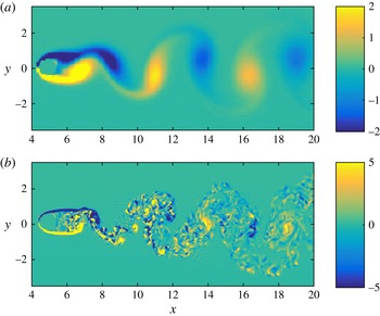
. Details of the three cases are provided in table 1. Figure 1 shows the spanwise vorticity component in the plane
 $z=0$
for the DNS at Reynolds number
 $Re=100$
and the LES at Reynolds number
 $Re=3900$
respectively. At Reynolds number
 $Re=100$
and due to the quasi two-dimensional configuration of the simulation, there are only few small-scale features. Most of the energy is gathered in the large-scale vortical structures. In this regime two topos modes are sufficient to reliably describe the flow. At Reynolds number
 $Re=3900$
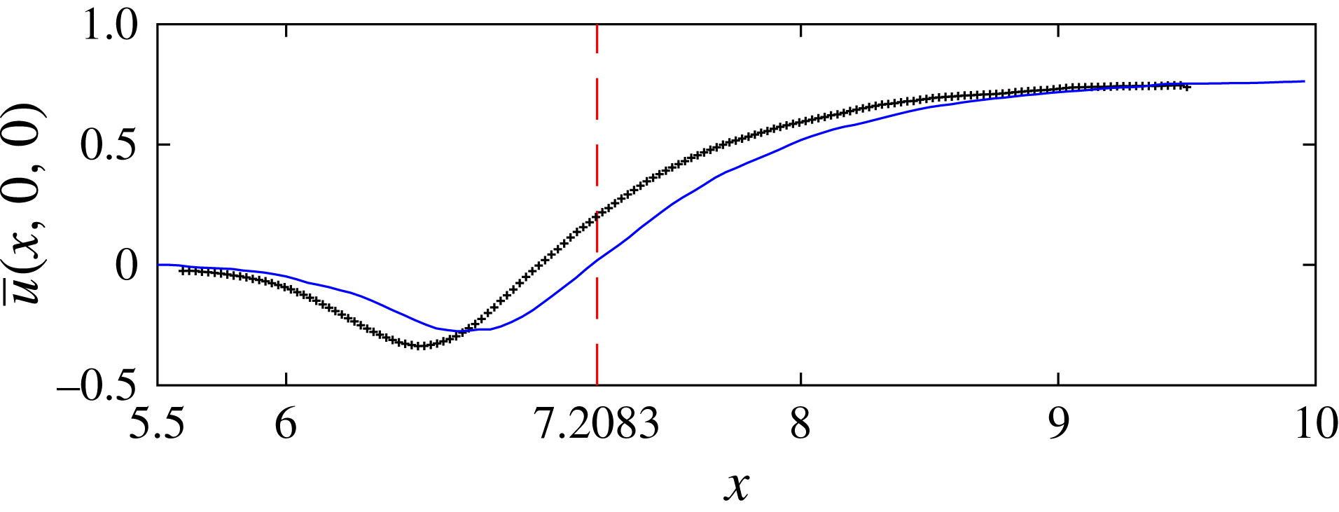
, a sustained turbulence can be observed in the far wake of the cylinder and in the recirculation zone just behind the cylinder. The boundary layer on the body is laminar and transition to turbulence takes place in the shear layers. The near-wake flow is mostly driven by those two shear layers (Ma, Karamanos & Karniadakis Reference Ma, Karamanos and Karniadakis2000). Their oscillations trigger the von Kármán vortex shedding and determine the size of the recirculation area. For this wake flow regime a higher number of modes must be retained. Figure 2 provides a test of the LES accuracy. There, we plotted the mean stream component of the velocity just after the cylinder in order to measure the length of the recirculation zone. To define it we here rely on the so-called bubble length. It is the distance between the base of the cylinder and the point with null longitudinal mean velocity (
 $\overline{u}=0$
) on the centreline of the flow (
 $y=0$
). Figure 2 shows a bubble length of approximately
 $1.7$
. This value is larger than experimental measurements (Parnaudeau et al.
Reference Parnaudeau, Carlier, Heitz and Lamballais2008) as expected with the classical Smagorinsky subgrid model (Chandramouli et al.
Reference Chandramouli, Heitz, Laizet and Mémin2016).
Spanwise vorticity component in a circular cylinder wake flow at Reynolds number: (a)
 $Re=100$
(DNS) and (b)
 $Re=3900$
(LES).

Mean stream velocity component in a circular cylinder wake flow at Reynolds number
 $Re=3900$
: (black crosses), particle image velocimetry (PIV) measurements (Parnaudeau et al.
Reference Parnaudeau, Carlier, Heitz and Lamballais2008); (blue line), LES used in this paper.

5 Diffusion modes results
We now apply the novel POD modelling, based on a stochastic small-scale representation as presented in § 3, to the cylinder flow configuration which is described in § 4. The reduced-order dynamics of the cylinder wake flow is known to be sensitive to the unresolved small-scale velocity component. In § 5.1, the small-scale energy and anisotropy are linked to small-scale diffusion modes. Assessment of the stochastic modelling is then performed in the following at the Reynolds number
 $Re=100$
and
 $Re=3900$
, respectively. In § 5.2, contributions of small-scale diffusion modes to large-scale flows are described and interpreted to determine which physical mechanisms of the wake flow are concerned. In § 5.3, we assess the performance of the subgrid term that was introduced by the stochastic representation of the small scales by comparing the chronos trajectories to the reference.
5.1 Estimation and decomposition of the turbulent velocity components
It can be noticed in the decomposition (3.11), that the diffusion modes
 $\unicode[STIX]{x1D66F}_{i}(x)$
are
 $d\times d$
symmetric matrices (with
 $\unicode[STIX]{x1D66F}_{i}=0$
for
 $i>0$
in the stationary case) at all spatial points. They can be diagonalized in a local orthonormal basis. Let us note however this decomposition does not ensure that
 $\unicode[STIX]{x1D656}(x,t)=\sum _{k=0}^{n}b_{k}(t)\unicode[STIX]{x1D66F}_{k}(x)$
is positive definite since
 $b_{i}(t)$
takes positive and negative values. In practice, though the stationary coefficient dominates largely the other coefficients (which gives a positive definite estimation), we would have to project the variance tensor on the manifold of positive definite matrices. In the following section, to analyse the small-scale energy and anisotropy we visualize the absolute values of the eigenvalues associated with the matrix modes,
 $\unicode[STIX]{x1D66F}_{i}$
. Due to chronos normalization, the variance tensor diffusion modes must also be normalized by the chronos’ square root eigenvalues
 $\sqrt{\unicode[STIX]{x1D706}_{i}}$
, as
 $$\begin{eqnarray}\displaystyle \tilde{\boldsymbol{a}}(x,t)=\mathop{\sum }_{k=0}^{n}\frac{b_{k}(t)}{\sqrt{\unicode[STIX]{x1D706}_{k}}}(\sqrt{\unicode[STIX]{x1D706}_{k}}z_{k}(x))\quad \text{and}\quad \frac{1}{T}\int _{0}^{\text{T}}\left(\frac{b_{k}}{\sqrt{\unicode[STIX]{x1D706}_{k}}}\right)^{2}=1\quad (\text{no sum on }k).\qquad & & \displaystyle\end{eqnarray}$$
We note that this normalization puts an even stronger emphasis on the stationary dissipation zero mode. Then, by (2.4) the corrective drift reads
 $$\begin{eqnarray}\displaystyle \boldsymbol{w}^{\star }-\boldsymbol{w}=\mathop{\sum }_{k=0}^{n}\frac{b_{k}(t)}{\sqrt{\unicode[STIX]{x1D706}_{k}}}(\boldsymbol{v}_{c})_{k}\quad \text{with }(\boldsymbol{v}_{c})_{k}=-\frac{1}{2}\unicode[STIX]{x1D735}\boldsymbol{\cdot }(\sqrt{\unicode[STIX]{x1D706}_{k}}\unicode[STIX]{x1D66F}_{k})^{\text{T}}\quad (\text{no sum on }k). & & \displaystyle\end{eqnarray}$$
Before dealing with chronos reconstruction, we propose in § 5.2 a new type of POD data analysis involving the information contained in the residual velocity. Algorithm 1 summarizes the steps of our data analysis, including the POD, the diffusion modes and the corrective drift computation.

5.2 Small-scale energy density, stationarity and anisotropy
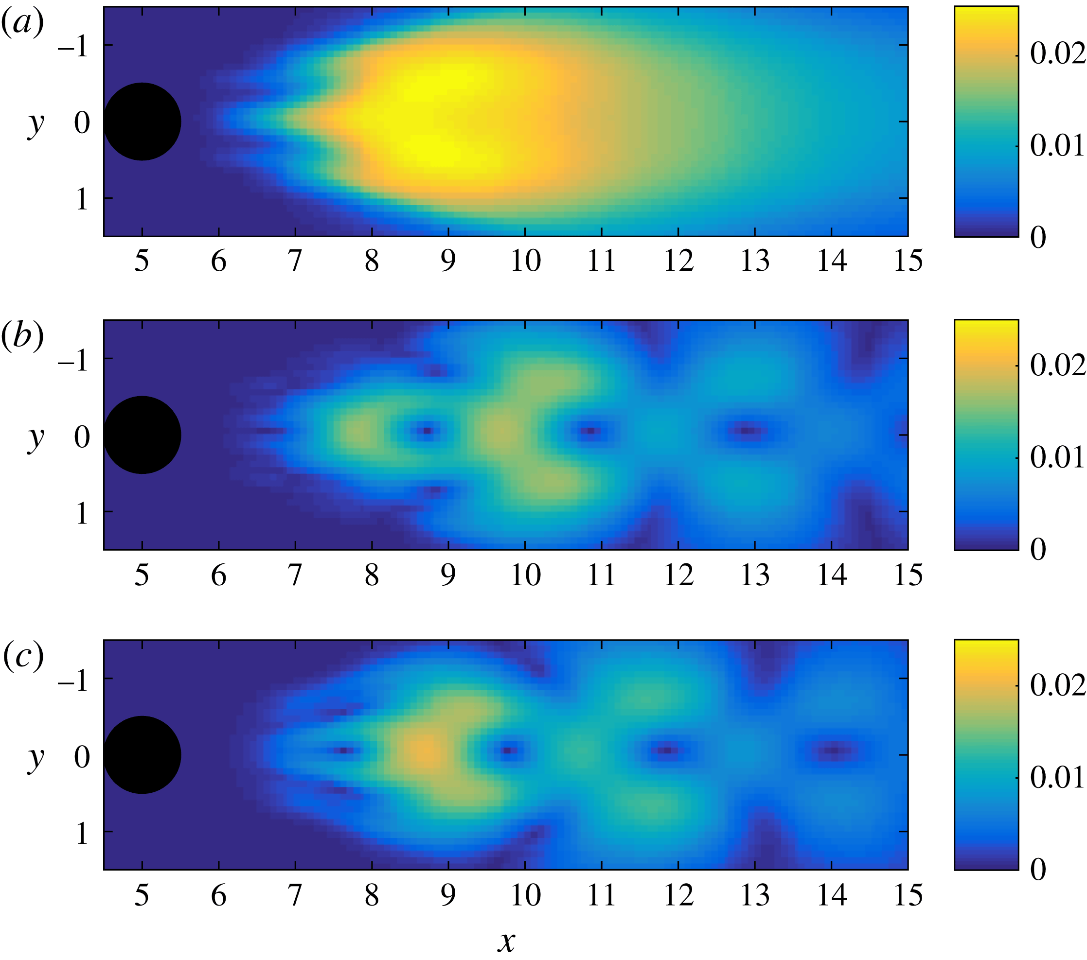
The turbulent kinetic energy density was computed by the sum of the diffusion modes eigenvalues, since small-scale TKE is represented (up to a time scale) by the norm of that tensor. The bigger the TKE, the more important is the diffusion of the resolved velocity by the small-scale velocity. The diffusion mode energies are plotted in figure 3(a–c) for the circular cylinder wake flow at
 $Re=100$
, with two POD modes and in the plane
 $z=0$
. The mode
 $\unicode[STIX]{x1D66F}_{0}$
yields regions of high TKE in the transitional region just downstream of the recirculation zone, i.e. for
 $7.5\leqslant x\leqslant 12$
. The other diffusion modes
 $\unicode[STIX]{x1D66F}_{1}$
and
 $\unicode[STIX]{x1D66F}_{2}$
work together since the two first chronos
 $b_{1}$
and
 $b_{2}$
are similar up to a phase difference. These diffusion modes are twice weaker than the stationary mode
 $\unicode[STIX]{x1D66F}_{0}$
. Their spatial patterns are more complex, although the large diffusion is still confined in the transitional region.
Local spectral representations of the matrix
 $\unicode[STIX]{x1D656}$
in a cylinder wake flow at
 $Re=100$
, for
 $n=2$
POD modes and in the plane
 $z=0$
. Turbulent kinetic energy of the diffusion modes: (a) diffusion mode
 $\unicode[STIX]{x1D66F}_{0}$
; (b) diffusion mode
 $\unicode[STIX]{x1D66F}_{1}$
; (c) diffusion mode
 $\unicode[STIX]{x1D66F}_{2}$
(square root of the sum of the squared eigenvalues).

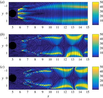
Local spectral representations of the matrix
 $\unicode[STIX]{x1D656}$
in a cylinder wake flow at
 $Re=100$
, for
 $n=2$
POD modes and in the plane
 $z=0$
. Small-scale anisotropy of the diffusion modes: (a) diffusion mode
 $\unicode[STIX]{x1D66F}_{0}$
; (b) diffusion mode
 $\unicode[STIX]{x1D66F}_{1}$
; (c) diffusion mode
 $\unicode[STIX]{x1D66F}_{2}$
(ratio of the absolute value of the largest eigenvalue to the absolute value of the smallest eigenvalue). The streamlines represent the first proper diffusion direction (i.e. the eigenvectors corresponding to the largest eigenvalues of the small-scale variance tensor).

To measure small-scale anisotropy, we computed the ratio between largest and smallest eigenvalues, corresponding to the condition number of the local small-scale velocity variances (see Algorithm 1). The bigger this quantity the more aligned toward the first local proper direction the small-scale velocity is, i.e. the more anisotropic the small-scale velocity and the diffusion of the resolved velocity are. Figure 4 shows the colour map of this quantity for the circular cylinder wake flow at
 $Re=100$
. In regions where the unresolved velocity component is largely anisotropic, the small-scale velocity is mainly directed towards the eigenvector which is associated with the largest eigenvalue of the small-scale variance tensor. The small-scale component imposes a diffusion of the resolved velocity in the same direction. The streamlines in figure 4 show the principal local diffusion directions defined by the largest eigenvectors. The orthogonal to the streamlines would depict the directions of least diffusion of the large-scale velocity by the small-scale component. These directions can be interpreted as those of lowest small-scale uncertainty. The streamlines clearly show the vortex formation region with the symmetric vortex rolling zone. The two pivotal locations at
 $y=\pm 0.5$
just before station
 $x=6$
where both shear layers start to roll into vortices are precisely indicated by high values of the small-scale anisotropy. The centreline of the recirculation zone (just before
 $x=6$
up to
 $x=7$
) is also associated with large anisotropy due to the alternation between formations of clockwise and anticlockwise vortices. After the transitional region (
 $x\geqslant 12$
), i.e. where regular and aligned vortices move downstream, the small-scale velocity anisotropy is maximum on the sides of the von Kármán vortex street (
 $x=\pm 1$
). This is due to the tails of the vortices visible in figure 1. This anisotropy is also visible in the non-stationary diffusion modes
 $\unicode[STIX]{x1D66F}_{1}$
and
 $\unicode[STIX]{x1D66F}_{2}$
.
Spanwise vorticity (a,c,e) and divergence (b,d,f) of the drift correction
 $-((\unicode[STIX]{x1D735}\boldsymbol{\cdot }\unicode[STIX]{x1D656})^{\text{T}})/2$
in a cylinder wake flow at
 $Re=100$
, for
 $n=2$
POD modes: (a,b) diffusion mode
 $\unicode[STIX]{x1D66F}_{0}$
; (c,d) diffusion mode
 $\unicode[STIX]{x1D66F}_{1}$
; (e,f) diffusion mode
 $\unicode[STIX]{x1D66F}_{2}$
.

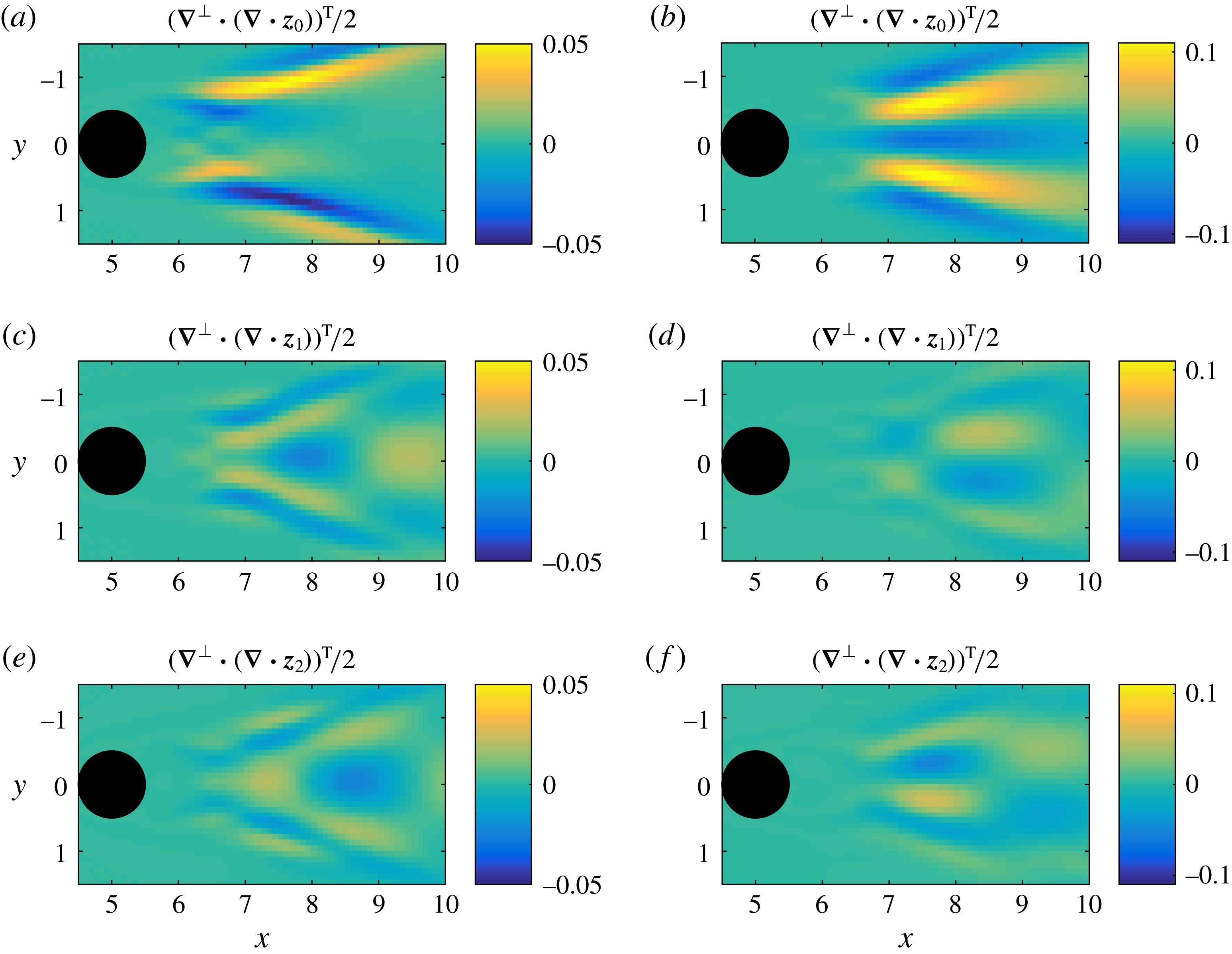
Another interesting feature of the small-scales stochastic representation principle concerns the emergence of the small-scale effective velocity (2.4), also called drift correction, related to the variance tensor inhomogeneity (see Algorithm 1 for the computation). Though at
 $Re=100$
, this contribution is weak as the flow is well captured with only two POD modes, it is nevertheless interesting to observed the velocity component that is induced by the neglected POD modes. In figure 5(a–f) we plot the vorticity and divergence of this advection correction term (2.4) for the diffusion modes
 $\unicode[STIX]{x1D66F}_{0}$
to
 $\unicode[STIX]{x1D66F}_{2}$
. The small-scale vorticity induced by the neglected modes is 2 orders of magnitude weaker than the whole flow vorticity (figure 1), which confirms its minor effect on the large-scale flow. However some interesting patterns emerge from these figures. In the vorticity map associated with the diffusion mode
 $\unicode[STIX]{x1D66F}_{0}$
(figure 5
a) we observe high divergence zones located at
 $6\leqslant x\leqslant 7$
with
 $y$
close to
 $\pm 0.5$
. In these regions where both shear layers roll into vortices, the vorticity drift correction due to the unresolved modes enhances the rolling process. Just downstream, at the boundaries of the shedding zone, elongated vorticity patterns can be observed. In the divergence map associated with the diffusion mode
 $\unicode[STIX]{x1D66F}_{0}$
(figure 5
b) we observe high divergence elongated zones located at
 $7\leqslant x\leqslant 9$
corresponding the trajectories of the launched vortices along which their sizes are increasing. Convergence zones are also shown at the same stations but between and on both sides of the divergence regions. Such flow corrections, albeit weak, take place in the region of the flow where physical mechanisms that give rise to vortex shedding are active and may have significant contributions if the flow is sensitive in these regions. One interesting feature, here, is the presence of high values of vorticity, corresponding to the maximum of anisotropy, at the two pivotal locations of the shear layers rolling into vortices. The non-stationary corrective advection is even weaker than the stationary one. The vorticity plots figure 5(c,e) unveil elongated vortices outside the recirculation zone but also relatively circular ones in the transitional region near the
 $x$
axis. In the divergence fields figure 5(c,e), large spots of convergence and divergence zones, odd with respect to the
 $x$
axis, appear in the end of the recirculation zone and in the transitional region.
Next it is of particular interest to analyse how the proposed small-scale stochastic modelling behaves with a more turbulent wake flow. So we consider the cylinder wake flow at Reynolds number
 $Re=3900$
.
Local spectral representation of the matrix
 $\unicode[STIX]{x1D656}$
in a cylinder wake flow at
 $Re=3900$
(LES), for
 $n=4$
POD modes: small-scale turbulent kinetic energy isosurfaces of the diffusion modes
 $\unicode[STIX]{x1D66F}_{0}$
–
 $\unicode[STIX]{x1D66F}_{4}$
, respectively. At places where the energy is high, the unresolved velocity and the diffusion are strong. The green isosurfaces are associated with higher values than the yellow isosurfaces (
 $0.007$
) and the blue isosurface (
 $0.08$
) corresponds to a higher value than the green isosurfaces (
 $0.03$
).

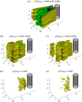
Figure 6 is a mapping of three-dimensional isosurfaces of the energy density for the diffusion modes
 $\unicode[STIX]{x1D66F}_{0}$
,
 $\unicode[STIX]{x1D66F}_{1}$
,
 $\unicode[STIX]{x1D66F}_{2}$
,
 $\unicode[STIX]{x1D66F}_{3}$
and
 $\unicode[STIX]{x1D66F}_{4}$
, in a cylinder wake flow at
 $Re=3900$
. We observe that the turbulent energy of the diffusion zero mode is approximately three times larger than for the non-stationary modes. These spatial small-scale energy distributions show that the largest magnitudes are reached at the end of the recirculation region and further downstream in the transitional region.
Local spectral representation of the matrix
 $\unicode[STIX]{x1D656}$
in a cylinder wake flow at
 $Re=3900$
(LES), for
 $n=4$
POD modes: Top (a,c,e) and side view (b,d,f) of the small-scale anisotropy isosurfaces of diffusion modes
 $\unicode[STIX]{x1D66F}_{0}$
(a,b),
 $\unicode[STIX]{x1D66F}_{1}$
(c,d) and
 $\unicode[STIX]{x1D66F}_{2}$
(e,f), respectively. This is the anisotropy of both the small-scale velocity statistics and of the diffusion of the large-scale velocity. The green surface (
 $\unicode[STIX]{x1D70E}=6$
) is associated with a higher anisotropy than the yellow surface (
 $\unicode[STIX]{x1D70E}=3$
). The red cones represent the preferential diffusion directions (i.e. the eigenvectors corresponding to the largest eigenvalues of the small-scale variance tensor). For the diffusion modes
 $\unicode[STIX]{x1D66F}_{1}$
(c,d) and
 $\unicode[STIX]{x1D66F}_{2}$
(e,f), these direction fields are spatially smoothed for an easier visualisation.

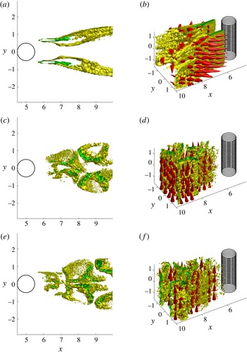
Let us now examine the small-scale anisotropy spatial distribution together with the arrows of the principal local diffusion directions plotted in figure 7. Figure 7(a,b) indicates that the stationary component of the turbulent diffusion of the resolved velocity is isotropic (i.e. shows a low anisotropy) in the centre of the von Kármán vortex street and further downstream whereas this stationary diffusion is anisotropic in the sides of the recirculation zone and of the von Kármán vortex street. There, the turbulent diffusion mostly acts along the plane perpendicular to the cylinder. The anisotropy maximums (highlighted by green surfaces in figure 7 a,b) reveals the two pivotal regions where the shear layers start to roll into vortices.
For
 $\unicode[STIX]{x1D66F}_{1}$
and
 $\unicode[STIX]{x1D66F}_{2}$
diffusion modes the structures of the non-stationary anisotropy are more complex (see figure 7
c,e), although large values are mainly confined inside the von Kármán vortex street. The associated non-stationary turbulent diffusion is preferentially in the spanwise direction. This behaviour can be related to the three-dimensionalization of the wake flow especially taking place along the spanwise direction in the transitional region. Our analysis gives an additional comprehension of this phenomena. In particular, the associated spanwise turbulent viscosity coefficient is found to be non-stationary.
Vorticity (a,c,e) and divergence (b,d
f) isosurfaces of the drift correction
 $-((\unicode[STIX]{x1D735}\boldsymbol{\cdot }\unicode[STIX]{x1D656})^{\text{T}})/2$
in a cylinder wake flow at
 $Re=3900$
, for
 $n=4$
POD modes: (a,b), diffusion mode
 $\unicode[STIX]{x1D66F}_{0}$
; (c,d), diffusion mode
 $\unicode[STIX]{x1D66F}_{1}$
; (e,f), diffusion mode
 $\unicode[STIX]{x1D66F}_{2}$
. In (a,c,e), the green isosurfaces are associated with a vorticity vector aligned downward whereas the yellow isosurfaces are associated with a vorticity vector aligned upward. In (b,d,f) the green surfaces stand for areas with isosurfaces which have negative divergence (convergent zone) whereas the yellow isosurfaces correspond to a positive divergence (divergent zone).

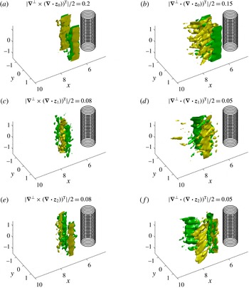
In figure 8(a,b), respectively the vorticity norm and the divergence of the stationary drift correction are plotted. Like for the
 $Re=100$
case, stationary vorticity and divergence corrections are observed near the shear layers, outside and at the end of the recirculation zone and just downstream in the launching area. Here again, high magnitudes of vorticity just downstream the maximum of anisotropy are associated with the two pivotal regions of the shear layers rolling into vortices. Nevertheless, the corrective vorticity is here stronger (one order of magnitude weaker than the global vorticity field). Other corrective vorticity structures can be observed at the end of the recirculation zone on the non-stationary modes
 $\unicode[STIX]{x1D66F}_{1}$
and
 $\unicode[STIX]{x1D66F}_{2}$
. The vorticity involved in those modes is approximately twice weaker than for the stationary diffusion mode. We identify
 $3$
and
 $4$
spanwise vortices in the corrective vorticity fields
 $(\unicode[STIX]{x1D735}\times (\unicode[STIX]{x1D735}\boldsymbol{\cdot }\unicode[STIX]{x1D66F}_{1})^{\text{T}})/2$
and
 $(\unicode[STIX]{x1D735}\times (\unicode[STIX]{x1D735}\boldsymbol{\cdot }\unicode[STIX]{x1D66F}_{2})^{\text{T}})/2$
respectively. As in the laminar case, divergence structures can be observed at the end of the recirculation zone and just downstream in the launching area. Again, these structures are odd with respect to the
 $x$
axis. Along the spanwise direction, periodic structures appear. Downstream no significant corrective velocities structures are observed, rather indicating a homogeneous character of the small-scale velocity and of the turbulent diffusion.
The diffusion modes analysis developed in the present paper identifies critical regions of the wake flow: the anisotropy mainly exhibits the pivotal location of the shear layers which are associated with large-scale vorticity corrections by the small-scale unresolved velocity and large-scale divergence corrections also take place in the vortex formation zone. For the wake flow considered, the results indicate that far enough downstream and outside the von Kármán vortex street boundaries an eddy-viscosity assumption is likely to be valid. However in the near wake or close to the von Kármán vortex street boundaries, such an assumption is too strong and corrective advection effects as well as structured energy dissipation effects must be taken into account. These findings support the recent results of Chandramouli et al. (Reference Chandramouli, Heitz, Laizet and Mémin2016) who demonstrated the significant contributions of such novel stochastic small-scale modelling in the context of coarse grid large eddy simulation of a wake flow.
5.3 Chronos reconstruction
In this section we aim at assessing the performance of the subgrid term introduced by the stochastic representation of the small scales. We compare the chronos trajectories that were directly reconstructed from the reduced-order dynamical system (3.13) to the observed chronos. Let us note that almost perfect long-time trajectories could be recovered through data-assimilation strategies (D’Adamo et al. Reference D’Adamo, Papadakis, Mémin and Artana2007; Artana et al. Reference Artana, Cammilleri, Carlier and Mémin2012; Cordier et al. Reference Cordier, Noack, Tissot, Lehnasch, Delville, Balajewicz, Daviller and Niven2013; Protas et al. Reference Protas, Noack and Östh2015). However, with such techniques it would be difficult to identify the intrinsic role of the subgrid scheme compared to a least-squares adaption of all the dynamics coefficients along the whole sequence. We therefore prefer to rely on a direct reconstruction strategy in which no identification, like least-squares or data-assimilation estimation procedures of the dynamical coefficients, is introduced. Note that such a direct reconstruction requires an additional stabilization, like a closure model, to ensure the long-term boundedness of the solution. In our model, the stabilization is inherited from the rigorously derived subgrid terms based on the variance of the unresolved velocity component. In the following, we compare temporal reconstructions obtained with our stochastic Galerkin model to those provided by different deterministic POD models.
The results presented so far on the diffusion mode analysis did not necessitate any knowledge of the Reynolds number to compute both the diffusion and the drift correction at the large scale by the unresolved small scale. We now turn to reduced-order dynamical systems which, in contrast, require the Reynolds value.
The modes energy mean,
 $\unicode[STIX]{x1D706}_{i}$
, and the topos,
 $\unicode[STIX]{x1D753}_{i}$
, are computed from the whole sequence of snapshots (
 $N=10\,000$
for
 $Re=100$
and
 $N=1,460$
for
 $Re=3900$
). As for the initial condition, we used the referenced values of the chronos, denoted
 $b_{i}^{ref}$
, computed directly from the snapshots covariance diagonalization. Then, regarding the chronos spectra, an optimal time subsampling
 $\unicode[STIX]{x0394}t$
is chosen, as explained in § 3.3. Afterwards, using the residual velocity and the chronos, the variance tensor,
 $\unicode[STIX]{x1D656}$
, is estimated. The coefficients of the reduced-order dynamical system of chronos (3.13) are directly computed using discrete derivation schemes. The chronos trajectories are simulated with a fourth-order Runge–Kutta integration method, with
 $b^{ref}(t=0)$
as initial condition and
 $\unicode[STIX]{x0394}t/10$
as simulation time step.
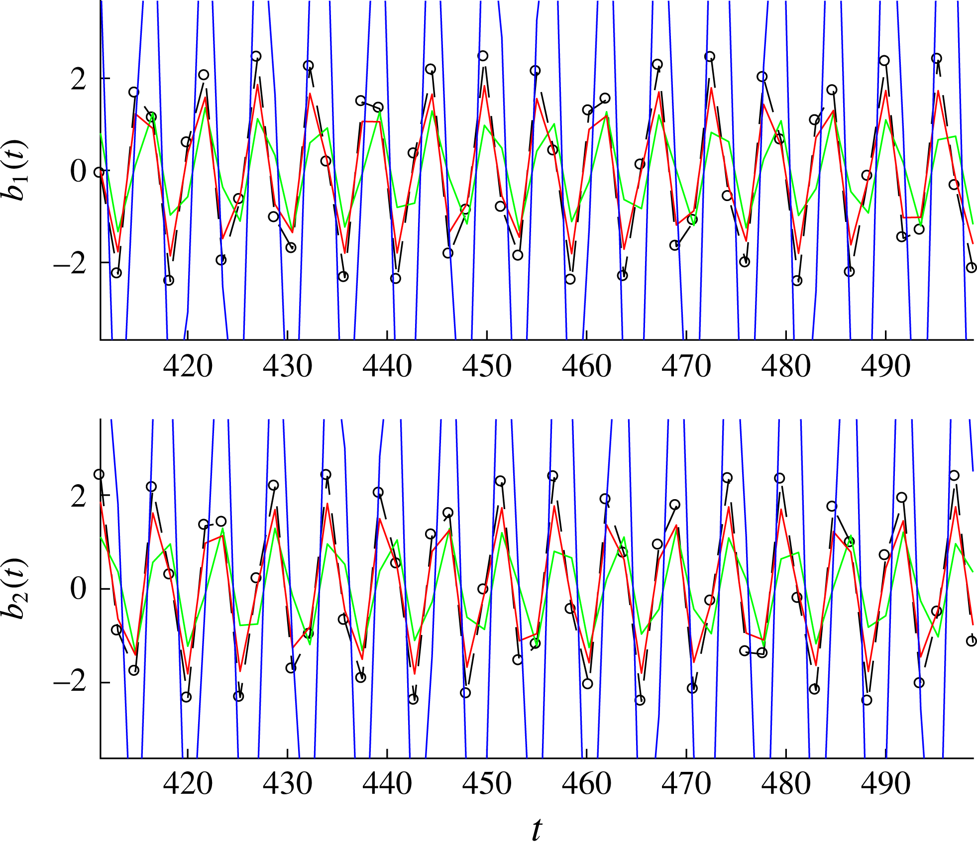
Reconstruction of the first two chronos for a wake flow at Reynolds number
 $Re=100$
, with
 $n=2$
POD modes and with a stationary variance tensor: (black dots), observed references; (blue line), standard POD–Galerkin; (red line), proposed stochastic representation; (green line), modal eddy-viscosity reduced-order model. The initial condition, at
 $t=0$
, is identical for all methods.

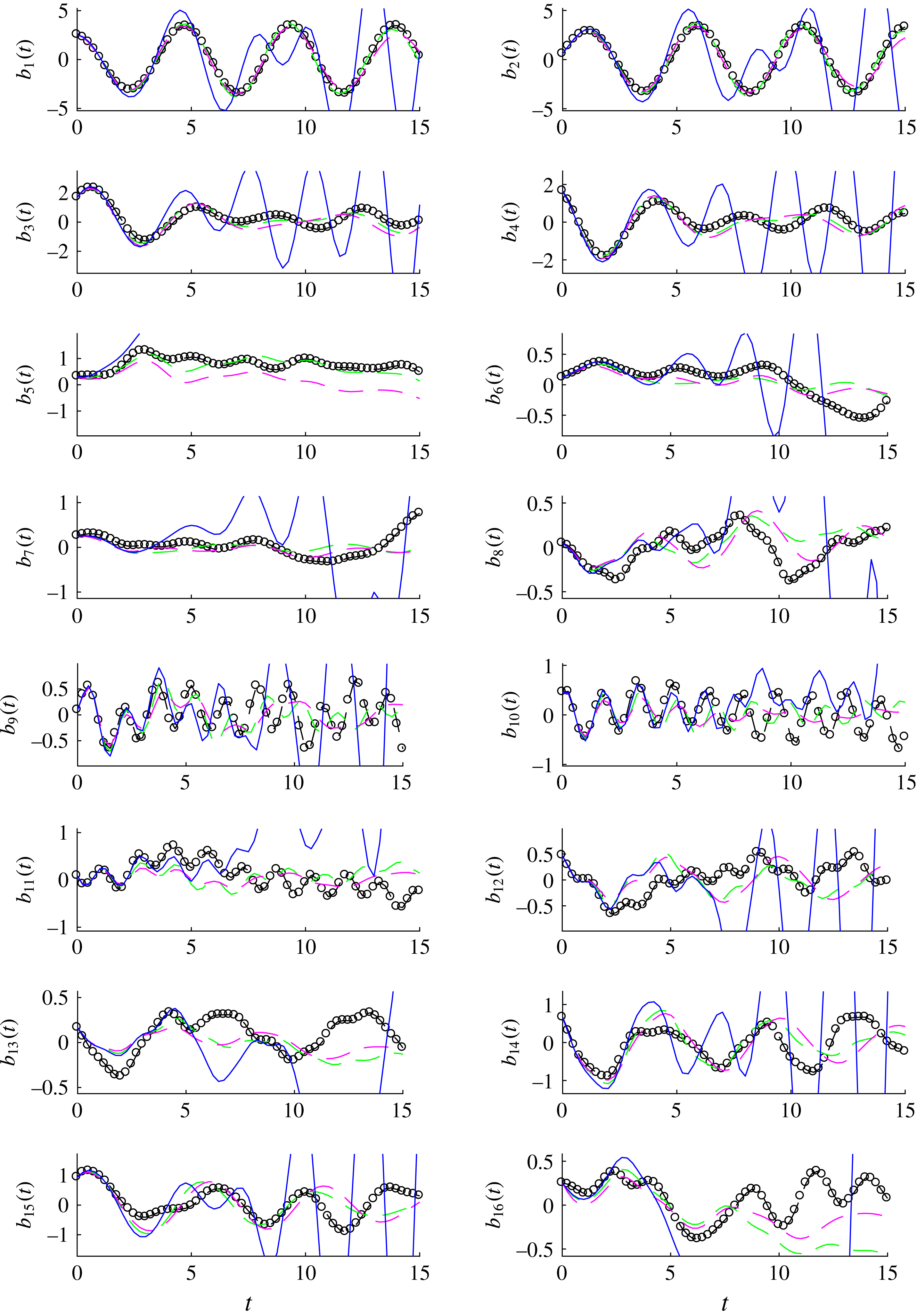
Reconstruction of the first ten chronos for a wake flow at Reynolds number
 $Re=3900$
(HR LES), with
 $n=16$
POD modes and with a variance tensor expressed as a linear function of the chronos and with modal characteristic times: (black dots), observed references; (blue line), standard POD–Galerkin; (dashed magenta line), proposed stochastic representation; (dashed green line), modal eddy-viscosity reduced-order model. The initial condition, at
 $t=0$
, is identical for all methods.

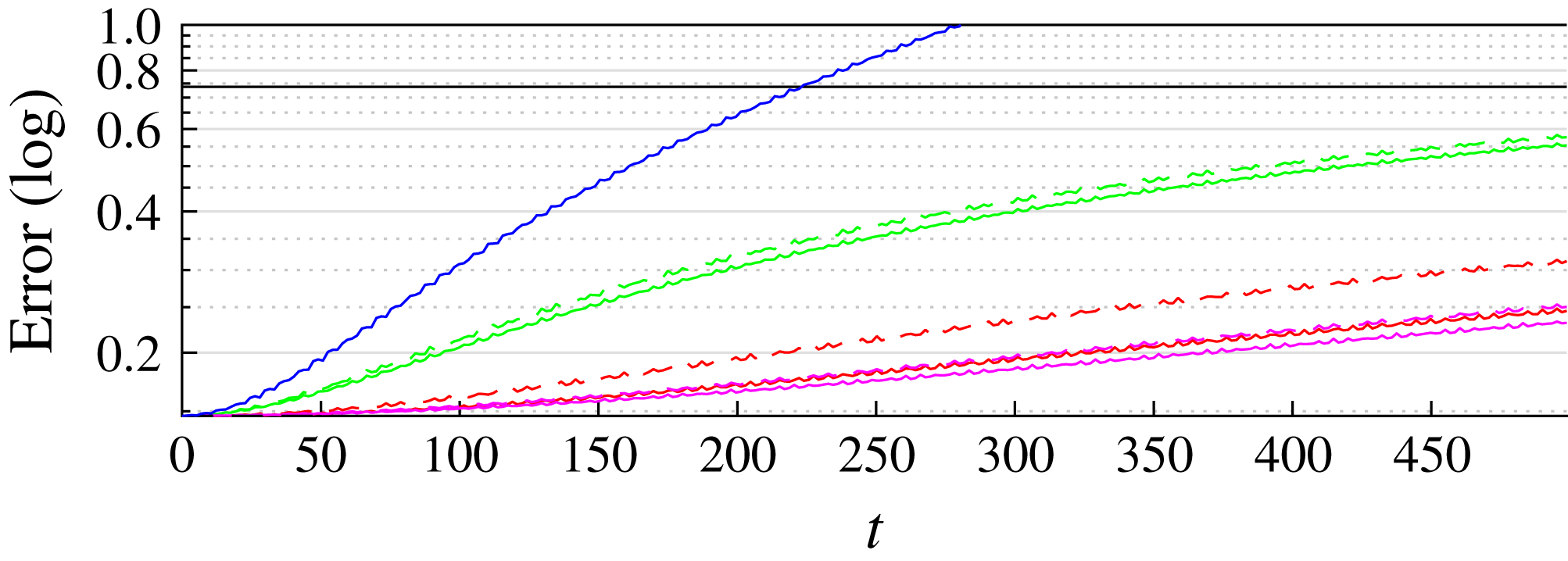
Normalized reconstruction error for a wake flow at Reynolds number
 $Re=100$
, with
 $n=2$
POD modes: (blue line), standard POD–Galerkin (without eddy viscosity); (red/magenta lines), proposed model with a stationary/non-stationary variance tensor, solid and dashed line with single and modal characteristic time, respectively; (green lines), solid and dashed with eddy-viscosity and modal eddy-viscosity reduced-order model, respectively. The modal eddy-viscosity coefficients are estimated through a least-squares fit on the whole data sequence. The dashed line indicates the error associated with the mode truncation:
 $\sum _{i=n+1}^{N}\unicode[STIX]{x1D706}_{i}$
. The black solid line is the error when we only consider the temporal mean velocity.

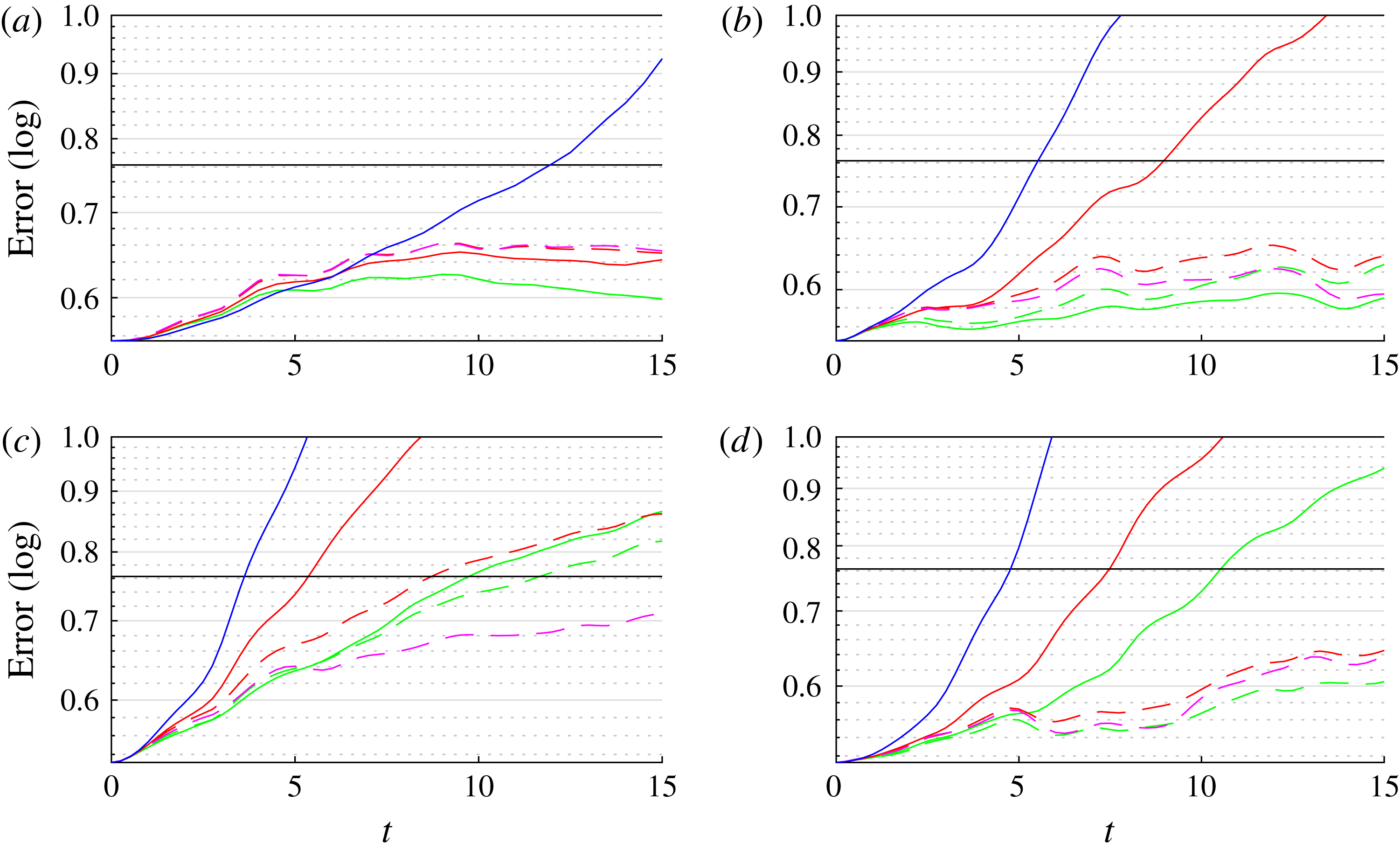
Normalized reconstruction error for a wake flow at Reynolds number
 $Re=3900$
(LES), with (from left to right and from top to bottom)
 $n=2$
, 4, 8 and 16 POD modes: (blue line), standard POD–Galerkin without eddy viscosity; (red/magenta lines), proposed model with a stationary/non-stationary variance tensor, solid and dashed line with single and modal characteristic time, respectively; (green lines), solid and dashed with eddy-viscosity and modal eddy-viscosity reduced-order model, respectively. The eddy-viscosity coefficients are estimated through a least-squares fit on the whole data sequence. The variance tensors are also estimated from a temporal mean on the whole sequence. The dashed line indicates the error associated with the mode truncation:
 $\sum _{i=n+1}^{N}\unicode[STIX]{x1D706}_{i}$
. The black solid line is the error when we only consider the temporal mean velocity.

Figures 9 and 10 show examples of the reconstruction of the chronos for
 $n=2$
at Reynolds number
 $Re=100$
and
 $n=16$
at Reynolds number
 $Re=3900$
, respectively, for the classical POD method (blue plot) and for the proposed modelling with respectively a stationary variance tensor (red line in figure 9) and a modal non-stationary variance tensor defined on the subspace associated with the chronos basis (dashed magenta line in figure 10) respectively. Each plot is sampled at the frequency
 $1/\unicode[STIX]{x0394}t$
. At Reynolds number
 $Re=100$
, the first two modes carry most of the energy. The references
 $b_{i}^{ref}$
(black plots) and the chronos obtained from an eddy-viscosity model are superimposed for comparison purposes. The eddy viscosity is optimally fitted by a least-squares estimation. It can be observed that our stochastic model follows the references quite well whereas the deterministic model blows up. Let us point out that here our reduced models are completely parameter free unlike the eddy-viscosity model. Figures 11 and 12 describe the error evolution along time. Approximating the square of the actual unresolved chronos by the time average of their squares, we defined the error as follows:
 $$\begin{eqnarray}\displaystyle \text{err}(t) & = & \displaystyle T\frac{\Vert \boldsymbol{v}^{ref}-\boldsymbol{v}\Vert _{L^{2}(\unicode[STIX]{x1D6FA})}}{\Vert \boldsymbol{u}^{ref}\Vert _{L^{2}(\unicode[STIX]{x1D6FA}\times [0,T])}},\nonumber\\ \displaystyle & = & \displaystyle T\frac{\mathop{\left\Vert \displaystyle \mathop{\sum }_{i=1}^{n}(b_{i}^{ref}-b_{i})\unicode[STIX]{x1D753}_{i}+\mathop{\sum }_{i=n+1}^{N}b_{i}^{ref}\unicode[STIX]{x1D753}_{i}\right\Vert }\nolimits_{L^{2}(\unicode[STIX]{x1D6FA})}}{\mathop{\left\Vert \displaystyle \mathop{\sum }_{i=0}^{N}b_{i}^{ref}\unicode[STIX]{x1D753}_{i}\right\Vert }\nolimits_{L^{2}(\unicode[STIX]{x1D6FA}\times [0,T])}},\nonumber\\ \displaystyle & {\approx} & \displaystyle \left(\frac{\displaystyle \mathop{\sum }_{i=1}^{n}(b_{i}^{ref}-b_{i})^{2}+\mathop{\sum }_{i=n+1}^{N}\unicode[STIX]{x1D706}_{i}}{\Vert \unicode[STIX]{x1D753}_{0}\Vert _{L^{2}(\unicode[STIX]{x1D6FA})}^{2}+\displaystyle \mathop{\sum }_{i=1}^{N}\unicode[STIX]{x1D706}_{i}}\right)^{1/2},\end{eqnarray}$$
which is greater than the minimal error associated with the modal truncation
 $$\begin{eqnarray}\displaystyle \text{err}(t)\geqslant \left(\frac{\displaystyle \mathop{\sum }_{i=n+1}^{N}\unicode[STIX]{x1D706}_{i}}{\Vert \unicode[STIX]{x1D753}_{0}\Vert _{L^{2}(\unicode[STIX]{x1D6FA})}^{2}+\displaystyle \mathop{\sum }_{i=1}^{N}\unicode[STIX]{x1D706}_{i}}\right)^{1/2}. & & \displaystyle\end{eqnarray}$$
Equation (5.14) defines the criterion error plotted in figures 11 and 12, whereas (5.15) constitutes a lower bound to this error. In figures 11 and 12, we successively display the error plots obtained for the standard POD–Galerkin model without subgrid dissipative term, for our model with stationary and non-stationary variance tensors, and finally for a deterministic modal eddy-viscosity model. This subgrid model, proposed in Rempfer & Fasel (Reference Rempfer and Fasel1994) consists in modifying the reduced-order system by adding a strong isotropic diffusive term (Laplacian) to stabilize the system. This eddy viscosity is said to be modal since different viscosity coefficients are attached to each chronos. Those coefficients are estimated by a least-squares fitting on the whole data sequence. Modal eddy viscosity in its least-squares form resembles indeed a data-assimilation strategy in which the best stationary isotropic dissipative forcing is estimated from the discrepancy between the model and the data. The same isotropic dissipation is imposed on the whole fluid domain at every time step. As such this subgrid dissipation is much more difficult to interpret in terms of local signatures of the small-scale coherent structures.
In figures 11 and 12, the dashed lines indicate the minimal error associated with the reduced subspace truncation error. The black solid line corresponds to the error level associated with the temporal mean velocity, i.e. setting all the chronos to
 $0$
. In this case,
 $$\begin{eqnarray}\displaystyle \text{err}_{|b=0}(t)\approx \left(\frac{\displaystyle \mathop{\sum }_{i=1}^{N}\unicode[STIX]{x1D706}_{i}}{\Vert \unicode[STIX]{x1D753}_{0}\Vert _{L^{2}(\unicode[STIX]{x1D6FA})}^{2}+\displaystyle \mathop{\sum }_{i=1}^{N}\unicode[STIX]{x1D706}_{i}}\right)^{1/2}. & & \displaystyle\end{eqnarray}$$
This term does not constitute an upper bound of the error. However, it provides the error level reached by the null model. In figures 11 and 12, fixing a log scale for the
 $y$
axis, we readily observe the exponential divergence of the standard POD reduced-order model (in blue).
We observe that even at Reynolds number
 $Re=100$
the modal eddy-viscosity model does not capture accurately, on a long-time period, the complex nonlinear dynamics undergone by the non-resolved modes (figure 11). The eddy-viscosity model over-damped the chronos, as shown in figure 9.
For the LES at Reynolds number
 $Re=3900$
(figure 12), we compared the eddy-viscosity approaches (modal and constant) with stationary and non-stationary models of the variance tensors. In this case the variance tensor as well as the eddy-viscosity coefficients have been estimated with
 $1,460\times \unicode[STIX]{x0394}t^{obs}/\unicode[STIX]{x0394}t$
vortex shedding cycles where
 $\unicode[STIX]{x0394}t^{obs}$
is the initial time step of the data (see table 1) whereas
 $\unicode[STIX]{x0394}t$
is the optimal subsampling time step given by the criterion (3.7). The performances of the modal and single characteristic times attached to the variance tensor have been evaluated and compared. The error plots are shown in figure 12. The introduction of different small-scale characteristic time steps associated with the different modes significantly improves the results that were obtained for a single common characteristic time. Both approaches are equivalent for short time period only. The introduction of modal characteristic times is clearly beneficial in the long run. The non-stationary representation performs better than the stationary one especially for
 $n=8$
modes. Indeed, due to its non-stationarity the associated reduced system is even better than eddy-viscosity models. Moreover, the piece of information brought by the non-stationary diffusion modes enables meaningful analysis of the small-scale contribution (see § 5.2). Except for
 $n=8$
modes, the modal eddy-viscosity approaches performs well. The constant eddy viscosity appears to only work when a small number of modes is involved. The (stationary or non-stationary) variance tensor models that are associated with modal characteristic time scales exhibit nearly the same stabilizing skills as the eddy-viscosity models (again excepting the case
 $n=8$
modes). Both models lead to similar error levels. Nevertheless, it must be outlined that the two approaches are based on different assumptions. Eddy viscosity relies intrinsically on a homogeneous isotropic diffusion with no preferential direction of energy dissipation. The diffusion remains constant whatever the considered region: in the near- or far-wake regions, and even in the shear layers. However, as a fixed constant estimated through a mean squares procedure, it provides the optimal amount of missing energy dissipation (with respect to a spatio-temporal mean of the squared norm) that is required to stabilize the reduced dynamical system. Conversely, as shown in the previous section, the variance tensor and the associated diffusion modes provide a finer representation of the small-scale action in terms of energy dissipation but also in terms of energy redistribution. As for the simulation of the reduced system, both models often lead to comparable error levels. They bring stability to the system in a similar way, but the variance tensor models unveil important clues on the small-scale flow structuration.
6 Conclusion
We investigated the study of reduced-order modelling based on a stochastic representation of the small scales proposed by Mémin (Reference Mémin2014) and Resseguier et al. (Reference Resseguier, Mémin and Chapron2017a ). This principle gives rise naturally to a drift correction generated by the inhomogeneity of the small-scale velocity variance and to an inhomogeneous diffusion term. The diffusion term is closely related to the eddy-viscosity assumption. Indeed, for an isotropic divergence-free random field, the stochastic representation boils down to the classical eddy-viscosity assumption. A POD–Galerkin projection of the corresponding stochastic Navier–Stokes equations provides a modified reduced-order dynamical system that includes a linear term gathering the effects of the effective advection and of the diffusion exerted by the unresolved small-scale component. This function directly depends on the small-scale variance that must be specified to close the system.
We proposed in this study a modelling based on the decomposition of this variance tensor on the chronos basis. The estimation has been performed on the residuals between the snapshots’ measurements and their resolved reconstruction on the topos basis. The coefficients of this decomposition quoted as the diffusion modes constitute meaningful features for the interpretation of the small-scale statistical organization. They allow us to examine in details the principal directions of the large-scale energy dissipation and also to extract advective structures both generated by the small-scale velocity.
The diffusion modes analysis has been applied to a circular cylinder wake flow. For this flow configurations in the laminar and in the subcritical regimes, the anisotropy of the diffusion modes determine regions of the flow that are key players. The largest magnitudes of the anisotropy zero mode (stationary mode) occur both in the vicinity of the pivotal zone of the shear layers rolling into vortices and also where the drift correction is effective.
Finally, the diffusion modes were coupled with modal characteristic time scales to provide a subgrid model. For wake flows, stabilizing skills are comparable to those obtained with optimally identified isotropic eddy-viscosity models. Such a stochastic approach consisting of a rigorously derived subgrid term may easily be applied to other turbulent flow configurations, for instance boundary layer flows that are known to develop complex multiscale mechanisms. Moreover, it will be interesting to see whether our proposed stochastic POD models could be used to design novel physics-based subgrid-scale models for LES approaches.
In order to obtain better chronos reconstruction results than that of an eddy-viscosity model, random forcings can be included – as in equation (2.5) – in the stochastic Navier–Stokes representation (2.8). This additional complexity maintains the variability of stable temporal modes. This full stochastic extension will be the subject of a next study. Other extensions of this methodology include online quantification of model errors for ensemble data-assimilation procedures. The authors are already pursuing these works in the context of reduced-order models but also in geophysical fluid dynamics (Yang & Mémin Reference Yang and Mémin2017; Resseguier et al. Reference Resseguier, Mémin and Chapron2017a ,Reference Resseguier, Mémin and Chapron b ).
Acknowledgements
The authors acknowledge the support of the SEACS project funded by the Brittany clusters of excellence (Cominslab, Lebesgue, and Mer). The authors thank Pranav Chandramouli for providing the data case at Reynolds
 $Re=3900$
.