1 Introduction
The instability of a stratified shear flow may play a key role in a variety of problems from geophysics to astrophysics. The most classical stability theory considers a horizontal mean flow that is sheared in the vertical plane. The stability problem is then described by the Taylor–Goldstein equation, with the celebrated Richardson-number criterion providing an important stability condition (Howard Reference Howard1961; Miles Reference Miles1961). A different paradigm has arisen more recently: the stability of flow that is sheared in the horizontal plane and rotating about a vertical axis. This alternative situation is the setting of the so-called strato-rotational instability, or ‘SRI’, and is relevant to oceanic currents, accretion disks and stratified Taylor–Couette experiments. SRI is different from Rayleigh’s centrifugal instability (which is conventionally argued to arise when the square of the angular momentum of a rotating flow decreases with radius), and has been ascribed to resonant mode interactions (Molemaker, McWilliams & Yavneh Reference Molemaker, McWilliams and Yavneh2001; Yavneh, McWilliams & Molemaker Reference Yavneh, McWilliams and Molemaker2001; Dubrulle et al. Reference Dubrulle, Marié, Normand, Richard, Hersant and Zahn2005; Shalybkov & Rüdiger Reference Shalybkov and Rüdiger2005; Le Bars & Le Gal Reference Le Bars and Le Gal2007; Park & Billant Reference Park and Billant2013; Ibanez, Swinney & Rodenborn Reference Ibanez, Swinney and Rodenborn2016; Leclercq, Nguyen & Kerswell Reference Leclercq, Nguyen and Kerswell2016). For the geometry of a channel of finite width, the conditions for resonance are restrictive, demanding that instability appears only for specific narrow bands of horizontal wavelength for which the phase velocities of the two uncoupled modes are nearly the same. (If the outer boundary is removed, and waves can freely radiate, the band of unstable wavelengths becomes continuous, as shown by Billant & Le Dizès (Reference Billant and Le Dizès2009) and Le Dizès & Billant (Reference Le Dizès and Billant2009); see also Le Dizès & Riedinger (Reference Le Dizès and Riedinger2010), who establish the connection between the resonant and radiative instabilities as the position of the outer boundary diverges.)
In the existing theory of SRI, the role of critical levels has usually been ignored. The classical critical level, where the phase speed
 $c$
of a wave matches the mean flow speed
 $U$
, introduces a singular point into the eigenvalue equations of linear theory and plays a central role in traditional shear-flow stability problems. For the SRI problem, another type of critical level appears where
 $(c-U)$
matches a characteristic internal-wave speed
 $N/k$
, where
 $N$
is the buoyancy (Brunt–Väisälä) frequency and
 $k$
is the streamwise wavenumber. This ‘baroclinic’ critical level again introduces singular points into the linear eigenvalue problem, but their impact on stability has not previously been considered in any detail. The only existing studies of the dynamics of baroclinic critical levels have focused on their effect on the local propagation of internal inertia–gravity waves through stratified shear flows (Olbers Reference Olbers1981; Basovich & Tsimring Reference Basovich and Tsimring1984; Badulin, Shrira & Tsimring Reference Badulin, Shrira and Tsimring1985; Staquet & Huerre Reference Staquet and Huerre2002).
Here, our goal is to explore how the presence of baroclinic critical levels affects the resonant mode interaction of SRI. For the task, we consider the model Couette channel flow of Dubrulle et al. (Reference Dubrulle, Marié, Normand, Richard, Hersant and Zahn2005) and Vanneste & Yavneh (Reference Vanneste and Yavneh2007) (amongst others). We use a combination of short-wavelength asymptotics and numerical solution of the linear eigenvalue problem, and examine how instability can arise through wave–mean-flow interaction from the perspective of conservation of pseudo-momentum. The model flow and governing equations, the normal-mode equation and the baroclinic critical level are described in § 2; the eigenvalue problem is solved in § 3 for relatively strong stratification, and then in § 4 for relatively weak stratification. The instability mechanism is examined via the concept of pseudo-momentum in § 5, and we conclude in § 6.
2 Mathematical formulation
2.1 Model and governing equations
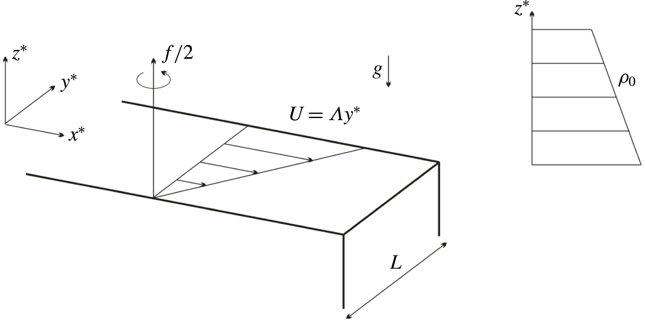
The geometry of the model flow is described by the Cartesian coordinate system
 $(x^{\ast },y^{\ast },z^{\ast })$
sketched in figure 1. The basic Couette flow
 $(\unicode[STIX]{x1D6EC}y^{\ast },0,0)$
is horizontal, where
 $\unicode[STIX]{x1D6EC}$
is the shear rate, and bounded by walls at
 $y^{\ast }=0$
and
 $y^{\ast }=L$
. The channel rotates around the
 $z^{\ast }$
-axis at the rate
 $f/2$
, and the fluid is stratified with buoyancy frequency
 $N$
. Here, the ‘
 $\ast$
’ notation is used to distinguish dimensional variables; to render the equations dimensionless, we use scales for velocity, time, length, density and pressure of
 $\unicode[STIX]{x1D6EC}L$
,
 $1/\unicode[STIX]{x1D6EC}$
,
 $L$
,
 $\unicode[STIX]{x1D70C}_{0}\unicode[STIX]{x1D6EC}^{2}L/g$
and
 $\unicode[STIX]{x1D70C}_{0}\unicode[STIX]{x1D6EC}^{2}L^{2}$
, respectively, where
 $\unicode[STIX]{x1D70C}_{0}$
is a reference density and
 $g$
is gravity. Thus, we set
 $(x,y,z)=L^{-1}(x^{\ast },y^{\ast },z^{\ast })$
and so forth, with the dimensionless variables appearing without the star decoration. The dimensionless rotation rate and Richardson number are
 $\unicode[STIX]{x1D6FA}=f/2\unicode[STIX]{x1D6EC}$
and
 $R=N^{2}/\unicode[STIX]{x1D6EC}^{2}$
. When
 $\unicode[STIX]{x1D6FA}>0$
(
 $\unicode[STIX]{x1D6FA}<0$
), the shear is anti-cyclonic (cyclonic). The Rayleigh discriminant of the base flow is
 $\unicode[STIX]{x1D6F7}=2\unicode[STIX]{x1D6FA}(2\unicode[STIX]{x1D6FA}-1)$
; we consider the regime where the flow is centrifugally stable,
 $\unicode[STIX]{x1D6F7}>0$
(
 $\unicode[STIX]{x1D6FA}>1/2$
or
 $\unicode[STIX]{x1D6FA}<0$
).
Sketch of the model geometry.

In the Boussinesq approximation, the linearized governing equations for the dimensionless perturbations to the velocity field
 $[u(x,y,z,t),v(x,y,z,t),w(x,y,z,t)]$
, pressure
 $p(x,y,z,t)$
and density
 $\unicode[STIX]{x1D70C}(x,y,z,t)$
are
 $$\begin{eqnarray}\displaystyle & \displaystyle u_{t}+yu_{x}+(1-2\unicode[STIX]{x1D6FA})v=-p_{x}, & \displaystyle\end{eqnarray}$$
 $$\begin{eqnarray}\displaystyle & \displaystyle v_{t}+yv_{x}+2\unicode[STIX]{x1D6FA}u=-p_{y}, & \displaystyle\end{eqnarray}$$
 $$\begin{eqnarray}\displaystyle & \displaystyle w_{t}+yw_{x}+\unicode[STIX]{x1D70C}=-p_{z}, & \displaystyle\end{eqnarray}$$
 $$\begin{eqnarray}\displaystyle & \displaystyle \unicode[STIX]{x1D70C}_{t}+y\unicode[STIX]{x1D70C}_{x}-Rw=0, & \displaystyle\end{eqnarray}$$
 $$\begin{eqnarray}\displaystyle & \displaystyle u_{x}+v_{y}+w_{z}=0, & \displaystyle\end{eqnarray}$$
where the subscripts denote partial derivatives. The boundary conditions are that there is no flow through the walls:
 $$\begin{eqnarray}\displaystyle v=0\quad \text{at}~y=0~\text{and}~y=1, & & \displaystyle\end{eqnarray}$$
and the channel is periodic in both
 $x$
and
 $z$
.
The linearized potential vorticity of the Boussinesq fluid is
 $$\begin{eqnarray}\displaystyle q=(2\unicode[STIX]{x1D6FA}-1)\unicode[STIX]{x1D70C}_{z}-R(v_{x}-u_{y}), & & \displaystyle\end{eqnarray}$$
and satisfies
 $$\begin{eqnarray}\displaystyle q_{t}+yq_{x}=0. & & \displaystyle\end{eqnarray}$$
For normal modes, this implies
 $q=0$
. In this circumstance, one can then formulate the conservation law (Vanneste & Yavneh Reference Vanneste and Yavneh2007):
 $$\begin{eqnarray}\displaystyle \frac{\text{d}}{\text{d}t}\int _{0}^{1}\mathsf{p}\,\text{d}y=0,\quad \mathsf{p}=\frac{1}{R}\overline{\unicode[STIX]{x1D70C}(w_{x}-u_{z})}, & & \displaystyle\end{eqnarray}$$
where
 $$\begin{eqnarray}\displaystyle \overline{(\cdots \,)}=\frac{1}{L_{x}L_{z}}\int _{0}^{L_{x}}\int _{0}^{L_{z}}(\cdots \,)\,\text{d}x\,\text{d}z. & & \displaystyle\end{eqnarray}$$
To second order in perturbation amplitude, the conserved integral in (2.9) corresponds to the net disturbance momentum in the streamwise direction, or the Eulerian pseudo-momentum (Bühler Reference Bühler2014). That is,
 $\mathsf{p}_{t}$
represents the acceleration of the mean flow by a normal mode at the cross-stream position
 $y$
, but (2.9) demands that the net effect vanishes, which places an important constraint on any unstable normal mode as we outline further in § 5.
2.2 Normal modes
We search for normal modes with the form,
 $$\begin{eqnarray}\displaystyle (u,v,w,p,\unicode[STIX]{x1D70C})=[\hat{u} (y),\hat{v}(y),{\hat{w}}(y),\hat{p}(y),\hat{\unicode[STIX]{x1D70C}}(y)]\exp (\text{i}kx+\text{i}mz-\text{i}\unicode[STIX]{x1D714}t)+\text{c.c.}, & & \displaystyle\end{eqnarray}$$
where ‘c.c.’ denotes the complex conjugate,
 $k$
and
 $m$
are the horizontal and vertical wavenumbers, the (complex) frequency is
 $\unicode[STIX]{x1D714}=\unicode[STIX]{x1D714}_{r}+\text{i}\unicode[STIX]{x1D714}_{i}$
and the corresponding streamwise phase speed is
 $c=\unicode[STIX]{x1D714}/k=c_{r}+\text{i}c_{i}$
. Note that from now on,
 $k$
,
 $m$
,
 $\unicode[STIX]{x1D714}$
and
 $c$
are dimensionless variables, in contrast to their dimensional counterparts referred to earlier in § 1. Substitution of this form into the linear equations followed by some algebraic manipulations leads to the eigenvalue equation (Vanneste & Yavneh Reference Vanneste and Yavneh2007),
 $$\begin{eqnarray}\displaystyle \frac{\text{d}^{2}\hat{u} }{\text{d}y^{2}}+h\frac{\text{d}\hat{u} }{\text{d}y}+l^{2}\hat{u} =0, & & \displaystyle\end{eqnarray}$$
where
 $$\begin{eqnarray}\displaystyle & \displaystyle h=\frac{2\unicode[STIX]{x1D707}^{2}k(2\unicode[STIX]{x1D6FA}-1)^{2}\hat{\unicode[STIX]{x1D714}}}{(\hat{\unicode[STIX]{x1D714}}^{2}-R)[\hat{\unicode[STIX]{x1D714}}^{2}-R-\unicode[STIX]{x1D707}^{2}(2\unicode[STIX]{x1D6FA}-1)^{2}]}, & \displaystyle\end{eqnarray}$$
 $$\begin{eqnarray}\displaystyle & \displaystyle l^{2}=-\unicode[STIX]{x1D706}^{2}=-k^{2}-\frac{\unicode[STIX]{x1D707}^{2}k^{2}}{\hat{\unicode[STIX]{x1D714}}^{2}-R}\left[\hat{\unicode[STIX]{x1D714}}^{2}-\unicode[STIX]{x1D6F7}+\frac{2(2\unicode[STIX]{x1D6FA}-1)\hat{\unicode[STIX]{x1D714}}^{2}}{\hat{\unicode[STIX]{x1D714}}^{2}-R-\unicode[STIX]{x1D707}^{2}(2\unicode[STIX]{x1D6FA}-1)^{2}}\right], & \displaystyle\end{eqnarray}$$
 $$\begin{eqnarray}\displaystyle \hat{\unicode[STIX]{x1D714}}=\unicode[STIX]{x1D714}-ky=k(c-y)\quad \text{and}\quad \unicode[STIX]{x1D707}=m/k. & & \displaystyle\end{eqnarray}$$
The boundary conditions on the channel walls become
 $$\begin{eqnarray}\displaystyle \hat{v}=\frac{\displaystyle m^{2}(2\unicode[STIX]{x1D6FA}-1)(y-c)\hat{u} +(\hat{\unicode[STIX]{x1D714}}^{2}-R)\frac{\text{d}\hat{u} }{\text{d}y}}{\text{i}k[\hat{\unicode[STIX]{x1D714}}^{2}-R-\unicode[STIX]{x1D707}^{2}(2\unicode[STIX]{x1D6FA}-1)^{2}]}=0\quad \text{at}~y=0~\text{and}~y=1. & & \displaystyle\end{eqnarray}$$
Because the eigenvalue problem is real, the eigenvalues
 $c$
and eigenfunctions
 $\hat{u} (y)$
are either real or appear as complex pairs. The equations have the symmetry,
 $(y,c)\leftrightarrow (1-y,1-c)$
, and so if we have one eigenfunction
 $\hat{u} (y)$
with eigenvalue
 $c$
, there is another solution pair,
 $\hat{u} (1-y)$
and
 $1-c$
.
If
 $\unicode[STIX]{x1D714}$
or
 $c$
is real, equation (2.12) has two singular points at
 $\hat{\unicode[STIX]{x1D714}}^{2}=R$
, corresponding to the ‘baroclinic critical levels’,
 $$\begin{eqnarray}\displaystyle y=y_{b\pm }\equiv c\pm \frac{\sqrt{R}}{k}. & & \displaystyle\end{eqnarray}$$
At these points, there is a regular Frobenius series solution
 $\hat{u} _{R}=1+O(y-y_{b\pm })$
, and a logarithmically singular one with
 $\hat{u} _{S}=\hat{u} _{R}\log |y-y_{b\pm }|+O(1)$
. Equation (2.12) also possesses two additional singular points where
 $\hat{\unicode[STIX]{x1D714}}^{2}=R+\unicode[STIX]{x1D707}^{2}(2\unicode[STIX]{x1D6FA}-1)^{2}$
, but these can be shown to be removable (Vanneste & Yavneh Reference Vanneste and Yavneh2007) and merit no further discussion. Note that the classical critical level,
 $y=y_{c}\equiv c$
, introduces no singularity in the current model given the constant shear of the basic flow profile.
In the following two sections, we solve the eigenvalue problem (2.12) both numerically and asymptotically to find unstable modes (
 $c_{i}>0$
). For the numerical computations, we use a shooting method based on the MATLAB function ODE15s, with trial guesses provided either by previous solutions at different parameter settings or the short-wavelength solutions. The calculated growth rates turn out to be relatively small (cf. Vanneste & Yavneh (Reference Vanneste and Yavneh2007)), and in setting up the problem for analysis, it is advantageous to examine the situation where
 $c_{i}\rightarrow 0$
.
In the limit of short vertical wavelength,
 $\unicode[STIX]{x1D707}^{2}\gg 1$
, where the character of the solutions is dictated by the sign of
 $l^{2}$
for
 $c_{i}\rightarrow 0$
, there are two configurations to consider depending on the sign of the factor,
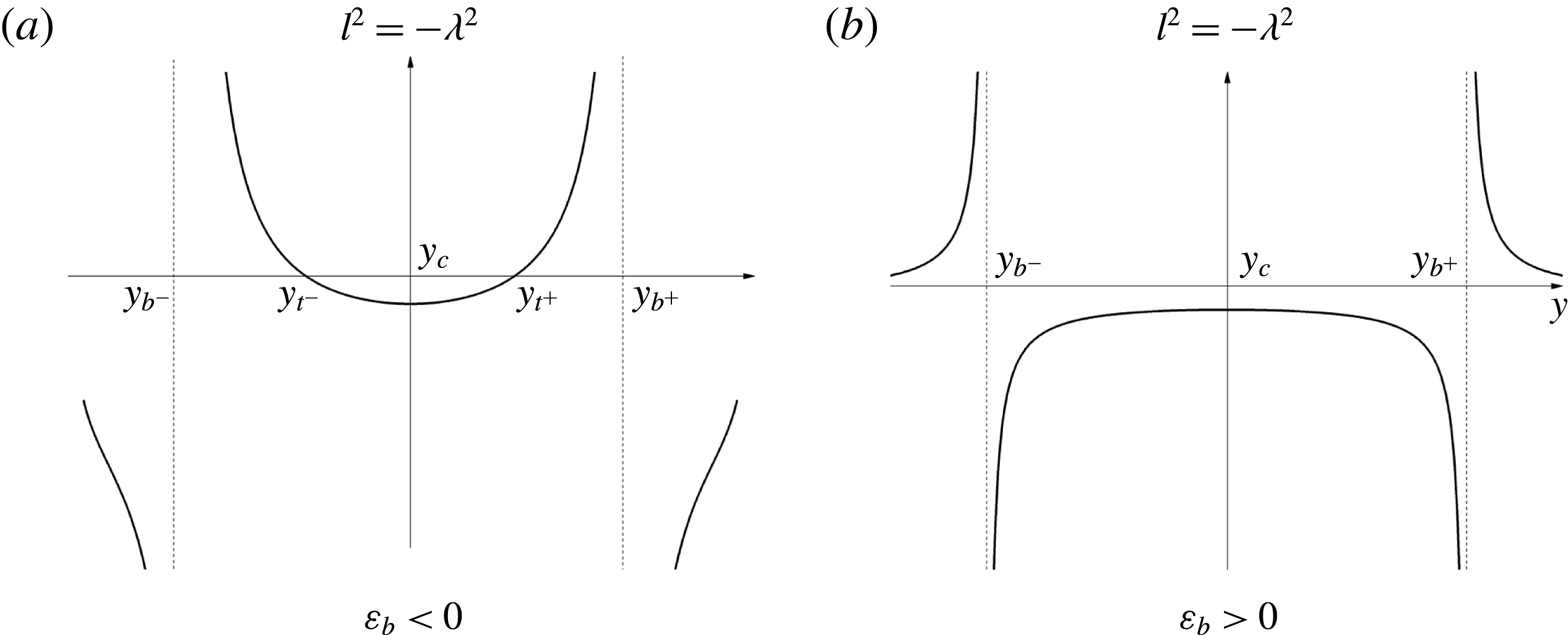
 $$\begin{eqnarray}\displaystyle \unicode[STIX]{x1D700}_{b}=\frac{2\sqrt{R}(2\unicode[STIX]{x1D6FA}-1)}{k[\unicode[STIX]{x1D707}^{2}(2\unicode[STIX]{x1D6FA}-1)(\unicode[STIX]{x1D6F7}-R)+2R]}, & & \displaystyle\end{eqnarray}$$
which determines the local behaviour near the baroclinic critical levels:
 $l^{2}\sim \pm [\unicode[STIX]{x1D700}_{b}(y-y_{b\pm })]^{-1}$
. The two configurations are illustrated in figure 2; if
 $\unicode[STIX]{x1D700}_{b}$
is negative, the evanescent region (
 $l^{2}<0$
) enclosing
 $y=y_{c}$
is bounded by two turning points
 $y_{t\pm }$
of the classical WKB-type where
 $l=0$
. The short-wavelength solutions have oscillatory character for
 $y_{t+}<y<y_{b+}$
and
 $y_{b-}<y<y_{t-}$
, with the baroclinic critical levels bounding the propagation zones. In §§ 3 and 4, special attention is given to modes with
 $\unicode[STIX]{x1D707}^{2}\gg 1$
. In this situation, our first configuration therefore applies to most geophysical conditions for which
 $N\gg |\,f|$
(
 $R\gg \unicode[STIX]{x1D6F7}$
). By contrast, when
 $\unicode[STIX]{x1D700}_{b}>0$
, the evanescent region is bounded by the baroclinic critical levels
 $y_{b\pm }$
, and the propagation zones occupy
 $y_{b+}<y<y_{t+}$
and
 $y_{t-}<y<y_{b-}$
. With
 $\unicode[STIX]{x1D707}^{2}\gg 1$
, this situation may apply to astrophysical disks where shear and rotation are relatively fast, so that
 $N\ll |f|$
. We consider the case with
 $\unicode[STIX]{x1D700}_{b}<0$
(which we refer to as stronger stratification) in § 3, and that with
 $\unicode[STIX]{x1D700}_{b}>0$
(denoted weaker stratification) in § 4. Note that, if
 $\unicode[STIX]{x1D707}^{2}$
is small or
 $\unicode[STIX]{x1D6FA}$
close to
 $1/2$
, the spatial structure of
 $l^{2}$
is more complicated than indicated in figure 2, in which case the configurations are less easily classified.
Plots of
 $l^{2}=-\unicode[STIX]{x1D706}^{2}$
against
 $y$
, illustrating the two configurations of interest for the spatial arrangements of the classical critical level
 $y=y_{c}$
, the turning points
 $y=y_{t\pm }$
and the baroclinic critical levels
 $y=y_{b\pm }$
, which are dictated by the sign of
 $\unicode[STIX]{x1D700}_{b}$
when
 $\unicode[STIX]{x1D707}^{2}\gg 1$
.

2.3 Solutions near the baroclinic critical levels
When we consider the eigenvalue problem in the short-wavelength limit, we take parameter settings such that some of the coefficients of (2.12) become relatively large. These choices also lead us to further analyse the solutions over a small region near the critical levels in the limit
 $|\unicode[STIX]{x1D700}_{b}|\ll 1$
(which is achieved below by taking
 $\unicode[STIX]{x1D707}^{2}\gg 1$
). Taking
 $y=y_{b+}$
by way of illustration, we set
 $$\begin{eqnarray}\displaystyle \unicode[STIX]{x1D702}=\frac{y-y_{b+}}{\unicode[STIX]{x1D700}_{b}} & & \displaystyle\end{eqnarray}$$
to find the leading-order local equation,
 $$\begin{eqnarray}\displaystyle \frac{\text{d}^{2}\hat{u} }{\text{d}\unicode[STIX]{x1D702}^{2}}+\frac{1}{\unicode[STIX]{x1D702}}\frac{\text{d}\hat{u} }{\text{d}\unicode[STIX]{x1D702}}+\frac{1}{\unicode[STIX]{x1D702}}\hat{u} =0. & & \displaystyle\end{eqnarray}$$
The two independent solutions of (2.20) are Bessel functions,
 $$\begin{eqnarray}\displaystyle & \displaystyle \hat{u} _{I}=\left\{\begin{array}{@{}ll@{}}\text{I}_{0}(2\sqrt{-\unicode[STIX]{x1D702}}), & \text{Re}(\unicode[STIX]{x1D702})\leqslant 0,\\ \text{J}_{0}(2\sqrt{\unicode[STIX]{x1D702}}), & \text{Re}(\unicode[STIX]{x1D702})\geqslant 0.\end{array}\right. & \displaystyle\end{eqnarray}$$
 $$\begin{eqnarray}\displaystyle & \displaystyle \hat{u} _{K}=\left\{\begin{array}{@{}ll@{}}\text{K}_{0}(2\sqrt{-\unicode[STIX]{x1D702}}), & \text{Re}(\unicode[STIX]{x1D702})\leqslant 0,\\ \displaystyle -\frac{\unicode[STIX]{x03C0}}{2}[\text{Y}_{0}(2\sqrt{\unicode[STIX]{x1D702}})+\text{i}\,\text{sgn}(\unicode[STIX]{x1D700}_{b})\text{J}_{0}(2\sqrt{\unicode[STIX]{x1D702}})], & \text{Re}(\unicode[STIX]{x1D702})\geqslant 0,\end{array}\right. & \displaystyle\end{eqnarray}$$
 $\sqrt{y-y_{b+}}$
to lie along the negative real axis, which leads to the inclusion of the sign of
 $\unicode[STIX]{x1D700}_{b}$
in (2.21b
), assuming that
 $c_{i}>0$
(for
 $c_{i}<0$
we replace this expression with the complex conjugate of
 $\hat{u} _{K}$
). Note that
 $\hat{u} _{I}$
corresponds to the regular Frobenius solution
 $\hat{u} _{R}$
, and
 $\hat{u} _{K}$
to the singular one
 $\hat{u} _{S}$
. Moreover,
 $\hat{u} _{I}$
grows exponentially away from the critical level for
 $\text{Re}(\unicode[STIX]{x1D702})<0$
, whereas
 $\hat{u} _{K}$
decays exponentially into that region; both solutions oscillate rapidly in space for
 $\text{Re}(\unicode[STIX]{x1D702})>0$
. These observations prepare the way for a match to the usual WKB solutions away from the baroclinic critical levels.
3 Instability of flow with stronger stratification
We first consider the case
 $\unicode[STIX]{x1D700}_{b}<0$
, which we refer to as a more strongly stratified flow because the situation is achieved in the short-wavelength limit,
 $\unicode[STIX]{x1D707}^{2}\gg 1$
, when
 $R>\unicode[STIX]{x1D6F7}$
(unless
 $\unicode[STIX]{x1D6FA}$
approaches
 $1/2$
). As illustrated in figure 2(a), we then expect modes to possess a wave-like character for
 $y_{b-}<y<y_{t-}$
and
 $y_{t+}<y<y_{b+}$
. We present results for unstable modes of the traditional SRI type that arise from a resonant coupling and have no baroclinic critical levels (
 $y_{b-}<0$
and
 $y_{b+}>1$
), and then describe how the form of this instability changes when one of these singular levels enters the channel.
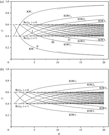
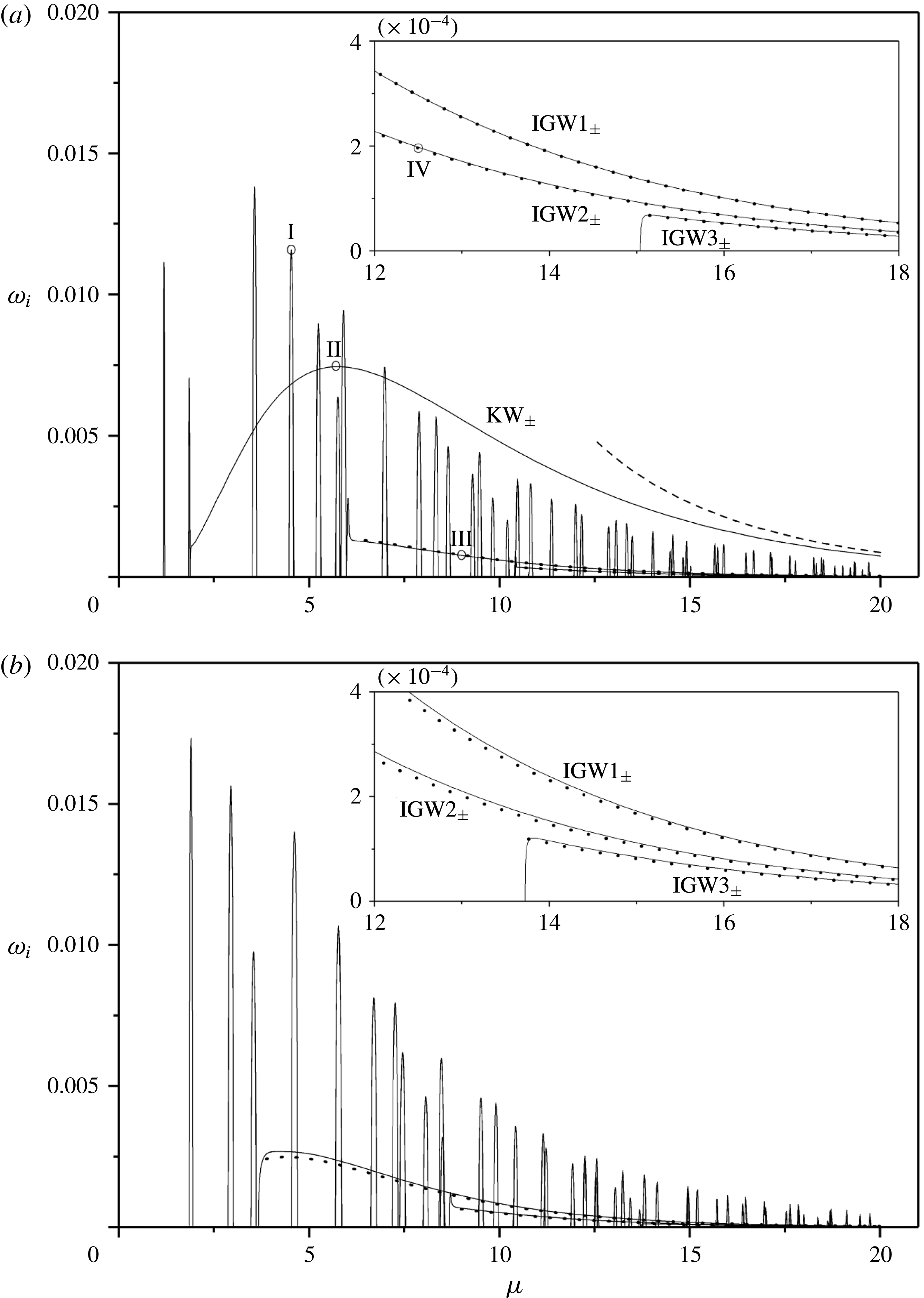
Figures 3 and 4 plot numerically calculated eigenvalues,
 $c_{r}$
and
 $c_{i}$
, against
 $\unicode[STIX]{x1D707}=m/k$
for two typical cases with anti-cyclonic (
 $\unicode[STIX]{x1D6FA}>0$
) or cyclonic (
 $\unicode[STIX]{x1D6FA}<0$
) shear (the specific examples have
 $R=9$
,
 $k=5$
and
 $\unicode[STIX]{x1D6FA}=5/8$
or
 $\unicode[STIX]{x1D6FA}=-1/8$
, implying
 $\unicode[STIX]{x1D6F7}=5/16$
). The two horizontal broken lines in the phase-speed plots of figure 3 indicate where a baroclinic critical level appears on the wall at
 $y=0$
or
 $y=1$
: the modes between the two lines do not have baroclinic levels in the domain; the modes above the line ‘
 $\text{Re}(y_{b-})=0$
’ have the critical level
 $y_{b-}$
, and the modes below the line ‘
 $\text{Re}(y_{b+})=1$
’ have the critical level
 $y_{b+}$
.
Phase speeds against
 $\unicode[STIX]{x1D707}=m/k$
for
 $R=9$
and
 $k=5$
, with (a)
 $\unicode[STIX]{x1D6FA}=5/8$
(anti-cyclonic shear) and (b)
 $\unicode[STIX]{x1D6FA}=-1/8$
(cyclonic shear). Eigenfunctions at the points I and II–IV are plotted in figures 5 and 6, respectively. The dotted line in (a) shows the asymptotic solution (3.7). The horizontal broken lines indicate the phase speeds for which modes develop baroclinic critical levels at the channel walls (
 $\text{Re}(y_{b-})=0$
and
 $\text{Re}(y_{b+})=1$
).

Unstable growth rates against
 $\unicode[STIX]{x1D707}=m/k$
for
 $R=9$
and
 $k=5$
, with (a)
 $\unicode[STIX]{x1D6FA}=5/8$
(anti-cyclonic shear) and (b)
 $\unicode[STIX]{x1D6FA}=-1/8$
(cyclonic shear). The insets show magnifications for higher
 $\unicode[STIX]{x1D707}$
and plot only the growth rates of the unstable modes generated by interaction with the baroclinic critical level. The dashed line in (a) shows the asymptotic solution (3.17); the dots in both panels show the asymptotic growth rates computed from (3.16). Eigenfunctions at the points I and II–IV are plotted in figures 5 and 6, respectively.

3.1 Resonant instabilities
When there are no baroclinic critical levels, modes can be classified as either Kelvin waves (KW) or internal gravity waves (IGW); see Vanneste & Yavneh (Reference Vanneste and Yavneh2007). The former are localized to one of the channel walls and decay exponentially into the interior of the flow; the latter are confined primarily to one of the propagation zones within the channel. We denote the Kelvin wave localized to the wall at
 $y=0$
(
 $y=1$
) by
 $\text{KW}_{-}$
(
 $\text{KW}_{+}$
). Similarly, an internal gravity wave confined to the wave cavity on the left (right) of
 $y=\text{Re}(y_{c})$
is referred to as
 $\text{IGW}_{-}$
(
 $\text{IGW}_{+}$
). There is only a single Kelvin wave associated with each of the channel walls, but the wave cavities support an infinite number of internal gravity waves; we distinguish the latter by adding an integer,
 $\text{IGW}n_{\pm }$
, corresponding to the number of nodes in
 $\text{Re}(\hat{u} )$
within the cavity. The main difference between the cases with anti-cyclonic and cyclonic shear is the presence of Kelvin modes with phase speeds within the range of the mean flow for the former.
As summarized by Vanneste & Yavneh (Reference Vanneste and Yavneh2007), resonant SRI arises when the phase speed of different
 $\text{KW}_{\pm }$
and
 $\text{IGW}_{\pm }$
modes lock together. This leads to a multitude of narrow bands of unstable wavenumbers, as illustrated by the sharp peaks in growth rate in figure 4. A sample unstable resonant mode is shown in figure 5, corresponding to the interaction of
 $\text{IGW}2_{+}$
and
 $\text{IGW}1_{-}$
(and indicated by point I in figures 3 and 4).
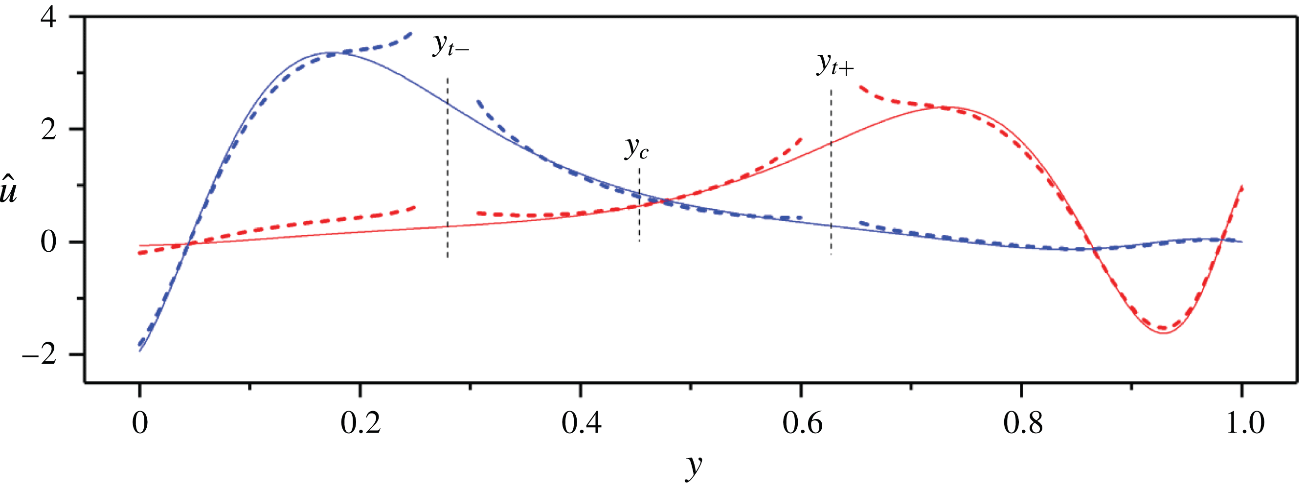
Eigenfunction
 $\hat{u}$
of the resonant unstable mode corresponding to the coupling of
 $\text{IGW2}_{+}$
and
 $\text{IGW1}_{-}$
(labelled by the point I in figures 3(a) and 4(a);
 $\unicode[STIX]{x1D707}=4.523$
). Red and blue lines represent real and imaginary part of the eigenfunction, respectively. The numerical solution is shown in solid lines, and has eigenvalue
 $c=0.454+0.00232\text{i}$
. The asymptotic eigenfunction is shown in dashed lines, and is constructed using the computed asymptotic eigenvalue
 $c\sim c_{0}+\unicode[STIX]{x0394}c\approx 0.453+0.00240\text{i}$
together with the formulae (3.1)–(3.4), which become inaccurate at the turning points
 $y=y_{t\pm }$
.

The details of the neutral modes and their unstable resonant interaction can be understood using WKB theory: in the region near
 $y=y_{c}$
,
 $-l^{2}=\unicode[STIX]{x1D706}^{2}>0$
and the decaying and growing solutions have (respectively) the exponential forms,
 $$\begin{eqnarray}\displaystyle \hat{u} _{-}=\frac{A}{\sqrt{\unicode[STIX]{x1D706}}}\exp \left[\int _{y}^{y_{t+}}\unicode[STIX]{x1D706}(y^{\prime })\,\text{d}y^{\prime }\right],\quad \hat{u} _{+}=\frac{A}{\sqrt{\unicode[STIX]{x1D706}}}\exp \left[\int _{y_{t-}}^{y}\unicode[STIX]{x1D706}(y^{\prime })\,\text{d}y^{\prime }\right]\quad \text{for}~y_{t-}<y<y_{t+}, & & \displaystyle \nonumber\\ \displaystyle & & \displaystyle\end{eqnarray}$$
where
 $$\begin{eqnarray}\displaystyle A=\exp \left[-\frac{1}{2}\int h(y)\,\text{d}y\right]=\sqrt{\left|\frac{\hat{\unicode[STIX]{x1D714}}^{2}-R-\unicode[STIX]{x1D707}^{2}(2\unicode[STIX]{x1D6FA}-1)^{2}}{\hat{\unicode[STIX]{x1D714}}^{2}-R}\right|}. & & \displaystyle\end{eqnarray}$$
Beyond the turning points (
 $y>y_{t+}$
or
 $y<y_{t-}$
, with
 $l^{2}>0$
), we apply the usual WKB turning-point connection formulae to find the oscillatory solutions,
 $$\begin{eqnarray}\displaystyle \hat{u} _{\pm }=\left\{\begin{array}{@{}ll@{}}\displaystyle \frac{2A}{\unicode[STIX]{x1D6F9}\sqrt{l}}\cos \left[\int _{y_{t\pm }}^{y}l(y^{\prime })\,\text{d}y^{\prime }\mp \frac{\unicode[STIX]{x03C0}}{4}\right], & y\gtrless y_{t\pm },\\ \displaystyle \frac{A}{\sqrt{l}}\cos \left[\int _{y_{t\mp }}^{y}l(y^{\prime })\,\text{d}y^{\prime }\mp \frac{\unicode[STIX]{x03C0}}{4}\right], & y\lessgtr y_{t\mp },\end{array}\right. & & \displaystyle\end{eqnarray}$$
where
 $$\begin{eqnarray}\displaystyle \unicode[STIX]{x1D6F9}=\exp \left[-\int _{y_{t-}}^{y_{t+}}\unicode[STIX]{x1D706}(y)\,\text{d}y\right]. & & \displaystyle\end{eqnarray}$$
Note that both
 $\hat{u} _{-}$
and
 $\hat{u} _{+}$
are real for real
 $c$
, indicating that they are both standing waves over this second region.
Given their respective exponential decay (
 $\hat{u} _{-}$
becomes exponentially small in
 $y>c$
and
 $\hat{u} _{+}$
in
 $y<c$
), the uncoupled
 $\pm$
modes therefore have phase speeds
 $c_{\pm }$
that are given only by the boundary condition
 $\hat{v}(y,c)=0$
at either
 $y=1$
or
 $y=0$
. That is,
 $$\begin{eqnarray}\displaystyle \hat{v}_{-}(0,c_{-})=0,\quad \hat{v}_{+}(1,c_{+})=0, & & \displaystyle\end{eqnarray}$$
where
 $$\begin{eqnarray}\displaystyle \hat{v}_{\pm }(y,c)=\frac{m^{2}(2\unicode[STIX]{x1D6FA}-1)(y-c)\hat{u} _{\pm }+(\hat{\unicode[STIX]{x1D714}}^{2}-R)\displaystyle \frac{\text{d}\hat{u} _{\pm }}{\text{d}y}}{\text{i}k[\hat{\unicode[STIX]{x1D714}}^{2}-R-\unicode[STIX]{x1D707}^{2}(2\unicode[STIX]{x1D6FA}-1)^{2}]} & & \displaystyle\end{eqnarray}$$
denotes the WKB eigenfunctions for the cross-stream velocity component
 $v$
. For
 $\text{KW}_{\pm }$
, a further reduction for
 $\unicode[STIX]{x1D707}\gg 1$
and
 $\unicode[STIX]{x1D6FA}>1/2$
with
 $c-y=O(\unicode[STIX]{x1D707}^{-1})$
furnishes the convenient expressions,
 $$\begin{eqnarray}\displaystyle c_{+}\approx 1-\frac{1}{m}\sqrt{\frac{2\unicode[STIX]{x1D6FA}R}{2\unicode[STIX]{x1D6FA}-1}}\quad \text{and}\quad c_{-}\approx \frac{1}{m}\sqrt{\frac{2\unicode[STIX]{x1D6FA}R}{2\unicode[STIX]{x1D6FA}-1}}, & & \displaystyle\end{eqnarray}$$
which are also plotted in figure 3(a).
Resonant mode coupling arises when the phase velocities of two basic modes
 $c_{-}$
and
 $c_{+}$
converge. The coupled modes comprise comparable proportions of
 $\hat{u} _{-}$
and
 $\hat{u} _{+}$
, and so the WKB solution for
 $\hat{u}$
is expressed by the linear combination,
 $$\begin{eqnarray}\displaystyle \hat{u} =C_{-}\hat{u} _{-}+C_{+}\hat{u} _{+}, & & \displaystyle\end{eqnarray}$$
for two constant
 $C_{\pm }$
. The boundary conditions then become
 $$\begin{eqnarray}\displaystyle C_{-}\hat{v}_{-}(0,c)+C_{+}\hat{v}_{+}(0,c)=C_{-}\hat{v}_{-}(1,c)+C_{+}\hat{v}_{+}(1,c)=0, & & \displaystyle\end{eqnarray}$$
implying the eigenvalue condition
 $$\begin{eqnarray}\displaystyle \hat{v}_{-}(0,c)\hat{v}_{+}(1,c)=\hat{v}_{+}(0,c)\hat{v}_{-}(1,c). & & \displaystyle\end{eqnarray}$$
The left-hand side of (3.10) combines the two leading-order dispersion relations in (3.5), whereas the right-hand side is exponentially small in view of the decay of
 $\hat{v}_{\pm }$
towards
 $y=0$
and
 $y=1$
, respectively. At resonance, the decoupled relations in (3.5) are satisfied simultaneously by
 $c_{+}=c_{-}=c_{0}$
. Treating the right-hand side of (3.10) as a small perturbation to the left-hand side (and neglecting the higher-order terms of the WKB approximation (3.1) and (3.3) that also correct
 $\hat{v}_{-}(0,c)$
and
 $\hat{v}_{+}(1,c)$
, but which are not expected to lead to instability), we can then estimate a correction
 $\unicode[STIX]{x0394}c$
to the leading-order eigenvalue
 $c_{0}$
, namely
 $$\begin{eqnarray}\displaystyle (\unicode[STIX]{x0394}c)^{2}\approx \frac{\hat{v}_{+}(0,c_{0})\hat{v}_{-}(1,c_{0})}{\hat{v}_{-,c}(0,c_{0})\hat{v}_{+,c}(1,c_{0})}, & & \displaystyle\end{eqnarray}$$
where the subscript ‘
 $c$
’ denotes a derivative of the eigenfunction with respect to the eigenvalue. In figure 5, the leading-order WKB eigenfunction and the corrected eigenvalue are compared satisfyingly with the corresponding numerical results for the sample mode of that figure. Note that, according to (3.9),
 $$\begin{eqnarray}\displaystyle \frac{C_{-}}{C_{+}}=-\frac{\hat{v}_{+}(0,c)}{\hat{v}_{-}(0,c)}\approx -\frac{\hat{v}_{+}(0,c_{0})}{\hat{v}_{-,c}(0,c_{0})\unicode[STIX]{x0394}c} & & \displaystyle\end{eqnarray}$$
which, because
 $\unicode[STIX]{x0394}c$
is purely imaginary for instability, implies a
 $\unicode[STIX]{x03C0}/2$
phase difference between the two coupled basic modes, as seen in figure 5.
3.2 Instability induced by the baroclinic critical level
As illustrated in figures 3 and 4, when modes develop baroclinic critical levels, the eigenvalue diagrams change dramatically in two key ways. First, the
 $\text{KW}_{-}$
and
 $\text{IGW}n_{-}$
(
 $\text{KW}_{+}$
and
 $\text{IGW}n_{+}$
) basic modes disappear above (below) the central band,
 $1-\sqrt{R}/k<c_{r}<\sqrt{R}/k$
, where they develop the
 $y_{b-}$
(
 $y_{b+}$
) critical level. This removes the possibility of any resonant mode interactions whenever there are baroclinic critical levels. Second, the same
 $\text{KW}_{-}$
and
 $\text{IGW}n_{-}$
(
 $\text{KW}_{+}$
and
 $\text{IGW}n_{+}$
) basic modes persist below (above) the central band,
 $1-\sqrt{R}/k<c_{r}<\sqrt{R}/k$
, even though they now develop the
 $y_{b+}$
(
 $y_{b-}$
) critical levels. More importantly, they become unstable over a wide band of wavenumbers. In figure 4(a), for the anti-cyclonic shear, four continuous lines of growth rate thereby appear for the
 $\text{KW}_{\pm }$
and
 $\text{IGW}n_{\pm }$
modes, with
 $n=1{-}3$
. The situation is the same for the cyclonic shear in figure 4(b), although the
 $\text{KW}_{\pm }$
modes are not present.
These observations can be translated into stability conditions in the limit of short vertical wavelength: resonant SRI requires the existence of the central band, or
 $k<2\sqrt{R}$
. For the
 $\text{IGW}n_{\pm }$
modes, we must further demand that
 $0<y_{t-}$
and
 $y_{t+}<1$
in order for wave-like regions to exist. But for
 $\unicode[STIX]{x1D707}\gg 1$
,
 $y_{t\pm }\approx c\pm \sqrt{\unicode[STIX]{x1D6F7}}/k$
. Thus, the SRI between
 $\text{IGW}n_{\pm }$
modes, which is the only possibility for cyclonic shear, requires
 $2\sqrt{\unicode[STIX]{x1D6F7}}<k<2\sqrt{R}$
(cf. Park & Billant Reference Park and Billant2013). For anti-cyclonic shear, the Kelvin waves (with
 $c_{-}>0$
or
 $c_{+}<1$
for
 $\unicode[STIX]{x1D707}\gg 1$
) can participate in unstable interactions, which modifies the condition for SRI to
 $k<2\sqrt{R}$
. By contrast, the instability of a
 $\text{KW}_{-}$
or
 $\text{IGW}n_{-}$
mode associated with a baroclinic critical layer requires
 $y_{b+}=c+\sqrt{R}/k<1$
(or equivalently,
 $y_{b-}=c-\sqrt{R}/k>0$
for a
 $\text{KW}_{+}$
or
 $\text{IGW}n_{+}$
mode). Hence, given that
 $c_{-}>0$
for
 $\text{KW}_{-}$
and
 $c_{-}>\sqrt{\unicode[STIX]{x1D6F7}}/k$
for
 $\text{IGW}n_{-}$
, the baroclinic critical layer instability requires
 $k>\sqrt{R}$
for anti-cyclonic shear and
 $k>\sqrt{R}+\sqrt{\unicode[STIX]{x1D6F7}}$
for cyclonic shear.
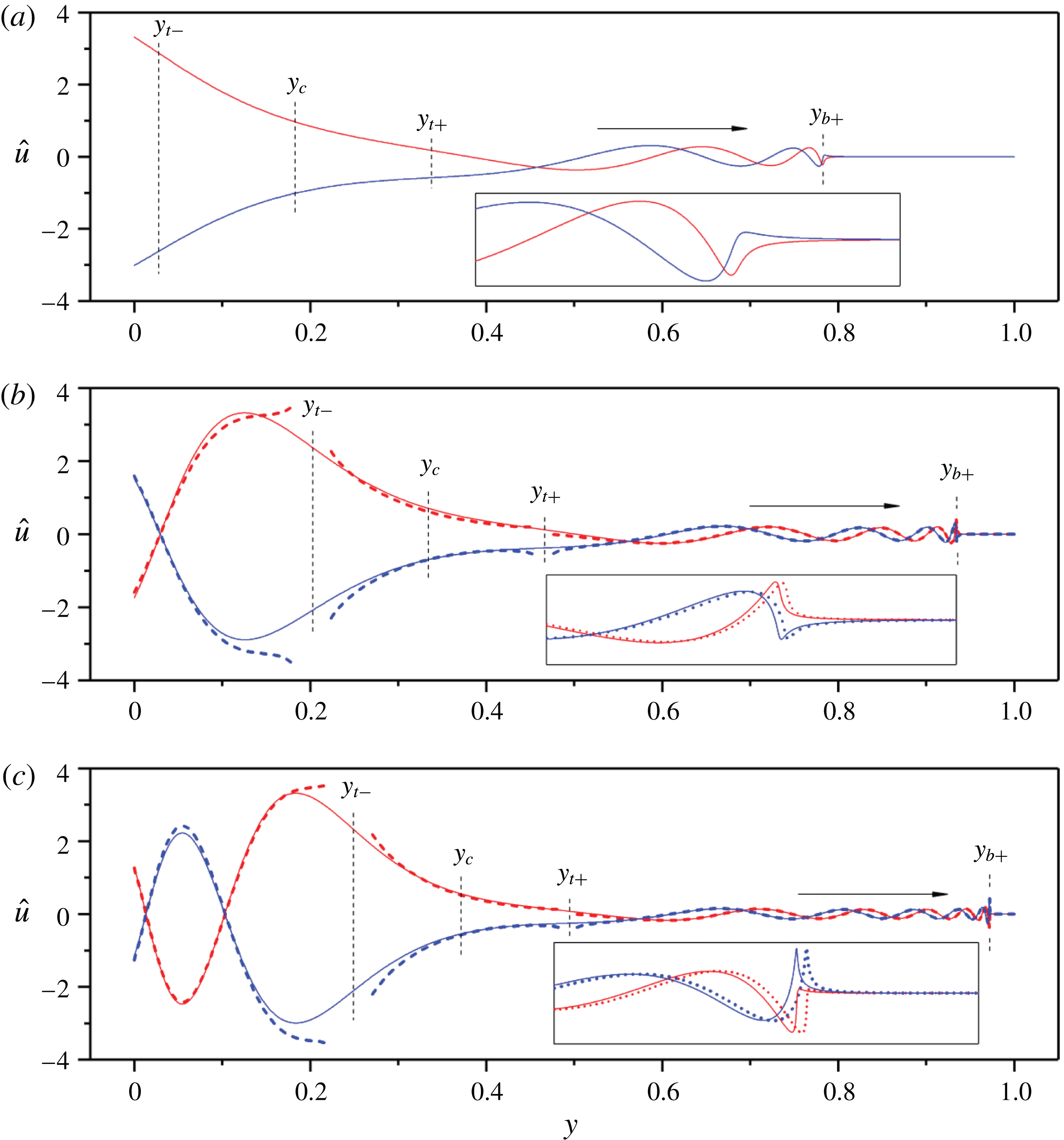
Eigenfunction
 $\hat{u}$
of unstable modes with baroclinic critical levels for
 $\unicode[STIX]{x1D6FA}=5/8$
and (a)
 $\text{KW}_{-}$
(
 $\unicode[STIX]{x1D707}=5.7$
; point II in figures 3 and 4), (b)
 $\text{IGW1}_{-}$
(
 $\unicode[STIX]{x1D707}=9$
; point III) and (c)
 $\text{IGW2}_{-}$
(
 $\unicode[STIX]{x1D707}=12.5$
; point IV). Red and blue lines represent real and imaginary parts of the eigenfunction, respectively. The solid lines show the numerical solutions. The corresponding results from WKB theory are shown as dashed lines, which become inaccurate at the turning points
 $y=y_{t\pm }$
(the asymptotic eigenfunction is not shown in (a) as the comparison is poor owing to the turning point
 $y=y_{t-}$
close to the boundary
 $y=0$
). In (b), numerical computations give
 $c=3.34\times 10^{-1}+1.54\times 10^{-4}\text{i}$
whereas the asymptotics indicate
 $c=3.35\times 10^{-1}+1.56\times 10^{-4}\text{i}$
. In (c), the numerical and asymptotic results are
 $c=3.71\times 10^{-1}+3.96\times 10^{-5}\text{i}$
and
 $c=3.72\times 10^{-1}+3.92\times 10^{-5}\text{i}$
, respectively. Insets show magnifications of the structure near the baroclinic critical levels.

Sample unstable modes are shown in figure 6, which plots the eigenfunctions of
 $\text{KW}_{-}$
,
 $\text{IGW}1_{-}$
and
 $\text{IGW}2_{-}$
at the points denoted II, III and IV in figures 3(a) and 4(a). For each mode, we see sharp structure in the eigenfunction near the baroclinic critical level
 $y_{b+}$
. To the right of these points, the mode amplitudes decay rapidly; to the left, the real part and imaginary parts have a
 $\unicode[STIX]{x03C0}/2$
phase difference indicative of travelling waves (propagating in the direction indicated by the arrows).
In WKB theory, the solution for the ‘
 $\pm$
’ mode is again dominated by the contribution from
 $\hat{u} _{\pm }$
near either
 $y=1$
or
 $y=0$
. To leading order, the phase velocity
 $c_{r}=c_{\pm }$
is again then given by one of (3.5). Focusing for the moment on the ‘
 $-$
’ mode, the solution is evanescent to the right of the critical level
 $y_{b+}$
. Provided the right-hand wall is sufficiently far from
 $y_{b+}$
, the solution is then
 $$\begin{eqnarray}\displaystyle \hat{u} =\frac{AC}{\sqrt{\unicode[STIX]{x1D706}}}\exp \left[-\int _{y_{b+}}^{y}\unicode[STIX]{x1D706}(y^{\prime })\,\text{d}y^{\prime }\right],\quad y_{b+}<y, & & \displaystyle\end{eqnarray}$$
with
 $C$
being an arbitrary constant. The exponential decay in (3.13) is fast given that
 $\unicode[STIX]{x1D706}\gg 1$
near the critical level, as seen in figure 6.
To the left of
 $y=y_{b+}$
, we exploit the large argument limits of Bessel function of the local solutions (2.21) to make the connection, which gives
 $$\begin{eqnarray}\displaystyle \hat{u} =\frac{AC}{\sqrt{l}}\exp \left\{\text{i}\left[\int _{y}^{y_{b+}}l(y^{\prime })\,\text{d}y^{\prime }+\frac{\unicode[STIX]{x03C0}}{4}\right]\right\},\quad y_{t+}<y<y_{b+}. & & \displaystyle\end{eqnarray}$$
That is, the eigenfunction now takes the form of a travelling wave over this region, unlike the standing-wave basic mode (which is exponentially small here). Given that the intrinsic frequency
 $\hat{\unicode[STIX]{x1D714}}=k(c-y)$
is negative in this region, the travelling waves propagate in
 $+y$
direction as indicated by the arrow in figure 6; i.e. they are incident on the critical level.
Over the same region,
 $y_{t+}<y<y_{b+}$
, the solution is also given by (3.8), and so to match with (3.14) we must take
 $$\begin{eqnarray}\displaystyle C_{-}=\text{i}C\unicode[STIX]{x1D6E9},\quad C_{+}=\frac{1}{2}C\unicode[STIX]{x1D6F9}\unicode[STIX]{x1D6E9},\quad \unicode[STIX]{x1D6E9}=\exp \left[\text{i}\int _{y_{t+}}^{y_{b+}}l(y)\,\text{d}y\right]. & & \displaystyle\end{eqnarray}$$
At
 $y=0$
, the leading-order boundary condition is
 $C_{-}\hat{v}_{-}(0,c)\sim 0$
, giving
 $c\sim c_{-}$
. An estimate of the correction
 $\unicode[STIX]{x0394}c$
to this eigenvalue then follows on keeping the next-order terms of
 $C_{-}\hat{v}_{-}(0,c)+C_{+}\hat{v}_{+}(0,c)=0$
and using (3.15):
 $$\begin{eqnarray}\displaystyle \unicode[STIX]{x0394}c\approx -\frac{C_{+}\hat{v}_{+}(0,c_{-})}{C_{-}\hat{v}_{-,c}(0,c_{-})}=\frac{\text{i}}{2}\unicode[STIX]{x1D6F9}\frac{\hat{v}_{+}(0,c_{-})}{\hat{v}_{-,c}(0,c_{-})} & & \displaystyle\end{eqnarray}$$
(ignoring higher-order corrections to the WKB approximation). The predictions computed from (3.16) for the
 $\text{IGW}n_{\pm }$
modes are included in figure 4 and again compare well with numerical computations. The WKB eigenfunction
 $\hat{u}$
and eigenvalue
 $c\sim c_{-}+\unicode[STIX]{x0394}c$
also match well with the numerical solutions for the two cases with higher
 $\unicode[STIX]{x1D707}^{2}$
shown in figure 6(b,c) (the caption reports the numerical and asymptotic results for
 $c$
).
In the limit
 $\unicode[STIX]{x1D707}\gg 1$
, we can again derive an explicit expression for
 $\text{KW}_{-}$
:
 $$\begin{eqnarray}\displaystyle c_{i}\approx c_{-}\exp \left(-2\int _{0}^{y_{t+}}\unicode[STIX]{x1D706}(y)\,\text{d}y\right). & & \displaystyle\end{eqnarray}$$
The prediction (3.17) is compared with the numerical results in figure 4(a).
4 Instability of flow with weaker stratification
If
 $\unicode[STIX]{x1D700}_{b}>0$
, we expect that the evanescent region around
 $y=\text{Re}(y_{c})$
is bounded by the baroclinic critical levels
 $y_{b\pm }$
(see figure 2
b); for
 $\unicode[STIX]{x1D707}^{2}\gg 1$
, this case is realized for
 $\unicode[STIX]{x1D6F7}>R$
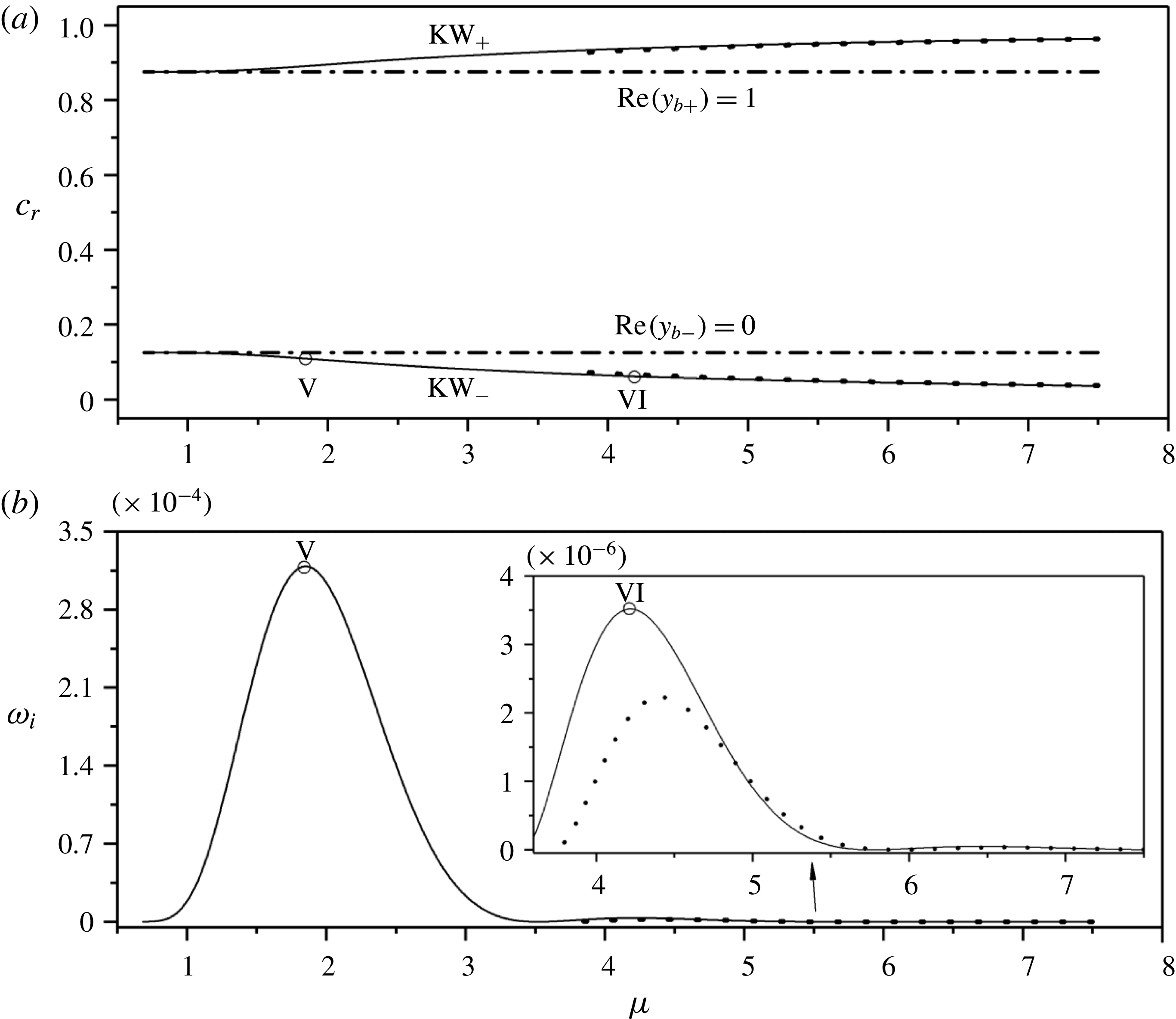
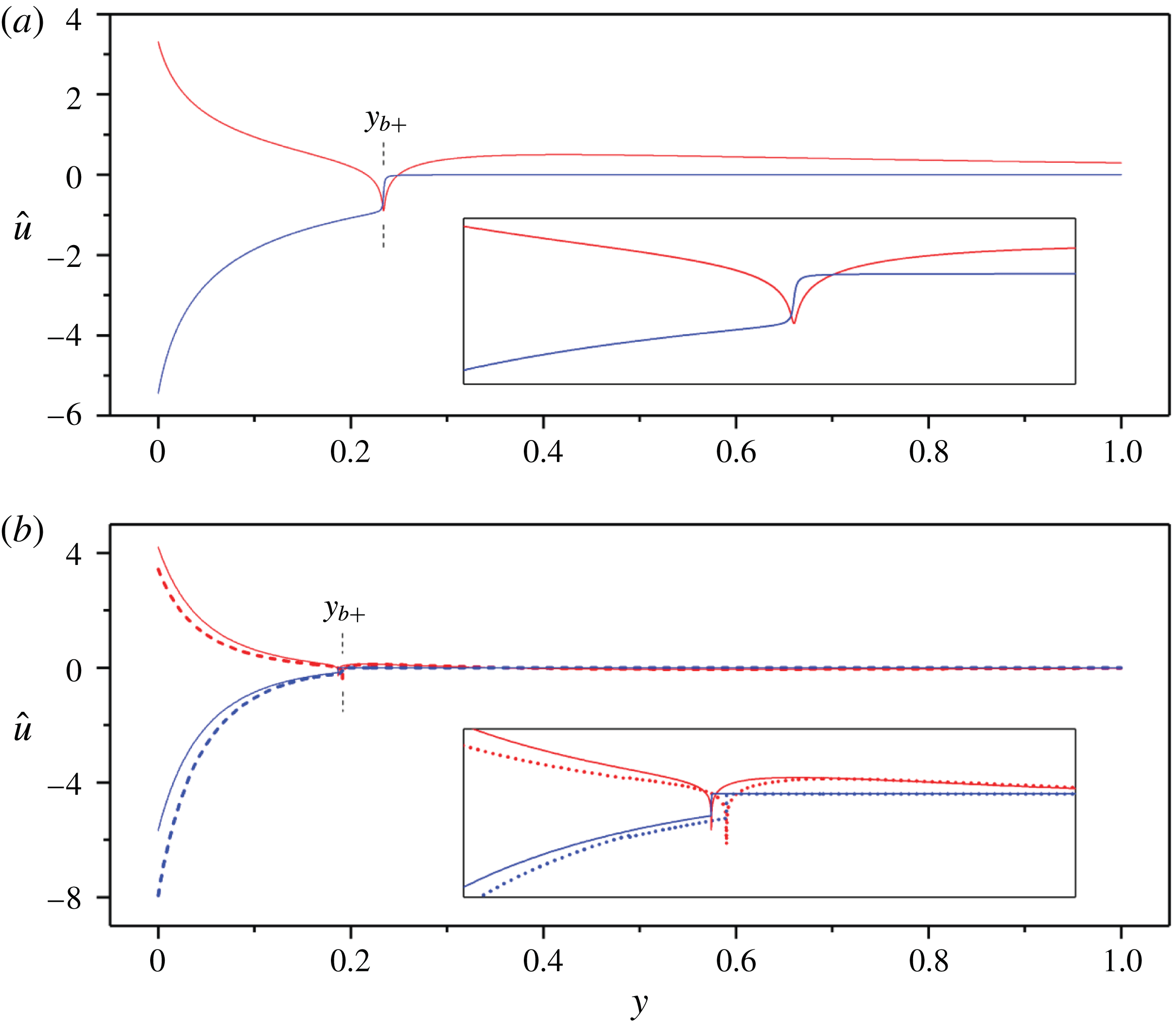
, and so corresponds to a more weakly stratified flow. In this situation, the exponential tail of a Kelvin wave riding on one of the channel walls can become transformed into internal waves beyond the adjacent critical level. If these internal waves can satisfy the boundary conditions at the other channel wall, a new type of normal mode is generated. Moreover, the interaction with that critical level destabilizes the mode via a mechanism that we shed light on later. The phase speed and growth rate of such solutions are plotted against
 $\unicode[STIX]{x1D707}$
in figure 7, with two sample eigenfunctions shown in figure 8.
(a) Phase speed
 $c_{r}$
and (b) growth rate
 $\unicode[STIX]{x1D714}_{i}$
against
 $\unicode[STIX]{x1D707}=m/k$
for
 $R=2.5\times 10^{-3}$
,
 $\unicode[STIX]{x1D6FA}=5/8$
and
 $k=0.4$
. The horizontal broken lines indicate where baroclinic critical levels appear at the channel walls. The dots plot the asymptotic results in (3.7) and (4.5) (which we do not include for the first peak in the main panel of (b) because the comparison is poor owing to the relatively small value for
 $\unicode[STIX]{x1D707}$
). Eigenfunctions at the points V and VI are plotted in figure 8.

Eigenfunction
 $\hat{u}$
of unstable modes with baroclinic critical levels at the points marked (a) V (
 $\unicode[STIX]{x1D707}=1.85$
) and (b) VI (
 $\unicode[STIX]{x1D707}=4.2$
) in figure 7. Red and blue lines represent real and imaginary parts of the eigenfunction, respectively. The solid line shows the numerical solution and the dashed line in (b) is the result of asymptotics (the asymptotic eigenfunction is not shown in (a) as the comparison is poor owing to the relatively small value for
 $\unicode[STIX]{x1D707}$
). The insets show magnifications of the structure near the baroclinic critical levels. In (b) the numerical result for the eigenvalue is
 $c=6.19\times 10^{-2}+8.82\times 10^{-6}\text{i}$
and
 $c=6.66\times 10^{-2}+5.30\times 10^{-6}\text{i}$
for the asymptotics.

In figure 7(a), the line ‘
 $\text{Re}(y_{b-})=0$
’ lies below that for ‘
 $\text{Re}(y_{b+})=1$
’ because
 $\sqrt{R}/k<0.5$
and the two Kelvin-wave speeds never intersect. Moreover, the critical levels remove any neutral internal waves with speeds inside the range of the base flow (which can be understood from the connection conditions across
 $y=y_{b\pm }$
implied by the local solutions derived in § 2.3:
 $\hat{u} _{K}$
possesses an exponentially decaying amplitude that corresponds to a travelling wave, which cannot satisfy the boundary condition). Thus, resonances do not occur, precluding traditional SRI. Instead, instability is generated purely through the interaction of the Kelvin waves with the baroclinic critical level. As seen in figure 8, to the right of
 $y_{b+}$
the unstable mode
 $\text{KW}_{-}$
takes the form of a standing wave, and there is an abrupt phase change across
 $y=y_{b+}$
.
For a short-wavelength description of the unstable
 $\text{KW}_{\pm }$
modes, we once more express the eigenfunction as a linear combination of decaying and growing solutions in the evanescent region,
 $\hat{u} =C_{-}\hat{u} _{-}+C_{+}\hat{u} _{+}$
, with constants
 $C_{-}$
and
 $C_{+}$
. Focusing again on
 $\text{KW}_{-}$
, in the evanescent region
 $0\leqslant y<y_{b+}$
,
 $\hat{u} _{-}$
and
 $\hat{u} _{+}$
are expressed by
 $$\begin{eqnarray}\displaystyle \hat{u} _{-}=\frac{A}{\sqrt{\unicode[STIX]{x1D706}}}\exp \left[\int _{y}^{y_{b+}}\unicode[STIX]{x1D706}(y^{\prime })\,\text{d}y^{\prime }\right],\quad \hat{u} _{+}=\frac{A}{\sqrt{\unicode[STIX]{x1D706}}}\exp \left[-\int _{y}^{y_{b+}}\unicode[STIX]{x1D706}(y^{\prime })\,\text{d}y^{\prime }\right],\quad 0\leqslant y<y_{b+}, & & \displaystyle \nonumber\\ \displaystyle & & \displaystyle\end{eqnarray}$$
with
 $A$
given by (3.2). Matching (4.1) to the local solution in (2.21), we can derive their corresponding expressions in
 $y>y_{b+}$
:
 $$\begin{eqnarray}\displaystyle \hat{u} _{-}=\frac{2A}{\sqrt{l}}\cos \left[\int _{y_{b+}}^{y}l(y^{\prime })\,\text{d}y^{\prime }-\frac{\unicode[STIX]{x03C0}}{4}\right],\quad \!\!\hat{u} _{+}=\frac{A}{\sqrt{l}}\exp \left[-\text{i}\int _{y_{b+}}^{y}l(y^{\prime })\,\text{d}y^{\prime }-\frac{\text{i}\unicode[STIX]{x03C0}}{4}\right],\quad \!\!y_{b+}<y\leqslant 1. & & \displaystyle \nonumber\\ \displaystyle & & \displaystyle\end{eqnarray}$$
The phase jump of
 $\hat{u} _{+}$
across the critical layer rationalizes that seen in the eigenfunction in figure 8.
For
 $\unicode[STIX]{x1D707}\gg 1$
, the boundary condition (2.16) on
 $y=1$
implies
 $\hat{u} =0$
to leading order, so the WKB solution in the oscillatory region
 $y_{b+}<y\leqslant 1$
is the standing gravity wave,
 $$\begin{eqnarray}\displaystyle \hat{u} =\frac{AC}{\sqrt{l}}\sin \int _{y}^{1}l(y^{\prime })\,\text{d}y^{\prime }\quad \text{for}~y_{b+}<y\leqslant 1, & & \displaystyle\end{eqnarray}$$
where
 $C$
is a constant. Reconciling (4.3) with the superposition of
 $\hat{u} _{\pm }$
in (4.2) implies
 $$\begin{eqnarray}\displaystyle C_{-}=-\frac{C}{2}\exp (-\text{i}\unicode[STIX]{x1D703}),\quad C_{+}=C\sin \unicode[STIX]{x1D703},\quad \unicode[STIX]{x1D703}=\int _{y_{b+}}^{1}l(y)\,\text{d}y+\frac{\unicode[STIX]{x03C0}}{4}. & & \displaystyle\end{eqnarray}$$
At the left boundary
 $y=0$
, the solution is dominated by
 $\hat{u} _{-}$
, leading to a basic phase speed
 $c_{-}$
which is again expressed by (3.7b
). The contribution of
 $\hat{u} _{+}$
is exponentially small, and keeping the next-order correction
 $\unicode[STIX]{x0394}c$
to the eigenvalue that it induces (again neglecting the potentially higher-order WKB approximations), provides the estimate,
 $$\begin{eqnarray}\displaystyle c_{i}\approx -\text{Im}\left[\frac{C_{+}\hat{v}_{+}(0,c_{-})}{C_{-}\hat{v}_{-,c}(0,c_{-})}\right]\approx 4c_{-}\cos ^{2}\left[\int _{y_{b+}}^{1}l(y)\,\text{d}y-\frac{\unicode[STIX]{x03C0}}{4}\right]\exp \left[-2\int _{0}^{y_{b+}}\unicode[STIX]{x1D706}(y)\,\text{d}y\right]. & & \displaystyle\end{eqnarray}$$
The prediction (4.5) is included in figure 7. Note the sinusoidal dependence of
 $c_{i}$
in (4.5) which is also evident in this figure.
At other parameter settings, a turning point
 $y_{t+}$
may intervene between the critical level
 $y_{b+}$
and the wall at
 $y=1$
. A further classical turning-point analysis must then be added to the WKB calculation, which adds an additional phase correction to (4.3). However, this leads to no significant change to the character of the unstable modes other than an exponential decay next to the wall, and warrants no additional discussion.
5 Implications of pseudo-momentum conservation
For the normal-mode form (2.11), the pseudo-momentum in (2.9) becomes
 $$\begin{eqnarray}\displaystyle \mathsf{p}=\hat{\mathsf{p}}(y)\text{e}^{2\unicode[STIX]{x1D714}_{i}t},\quad \hat{\mathsf{p}}(y)=\frac{(\unicode[STIX]{x1D707}\hat{u} ^{\ast }-{\hat{w}}^{\ast }){\hat{w}}}{y-c}+\text{c.c.},\quad {\hat{w}}=-\frac{\unicode[STIX]{x1D707}\hat{\unicode[STIX]{x1D714}}\left[(2\unicode[STIX]{x1D6FA}-1)\displaystyle \frac{\text{d}\hat{u} }{\text{d}y}-k\hat{\unicode[STIX]{x1D714}}\hat{u} \right]}{k[\hat{\unicode[STIX]{x1D714}}^{2}-R-\unicode[STIX]{x1D707}^{2}(2\unicode[STIX]{x1D6FA}-1)^{2}]}, & & \displaystyle\end{eqnarray}$$
where the
 $\ast$
superscript denotes complex conjugation. Thus the conservation law (2.9) reduces to
 $$\begin{eqnarray}\displaystyle 2\unicode[STIX]{x1D714}_{i}\int _{0}^{1}\hat{\mathsf{p}}(y)\,\text{d}y=0. & & \displaystyle\end{eqnarray}$$
This condition places no constraint on the spatial structure of neutral modes with
 $\unicode[STIX]{x1D714}_{i}=0$
. However, unstable modes with
 $\unicode[STIX]{x1D714}_{i}\neq 0$
must have zero total pseudo-momentum
 $\int _{0}^{1}\hat{\mathsf{p}}(y)\,\text{d}y=0$
. This demands that the spatial structure of the modes, as characterized by the density
 $\hat{\mathsf{p}}(y)$
, must break down into cancelling contributions from regions of opposite sign of pseudo-momentum.
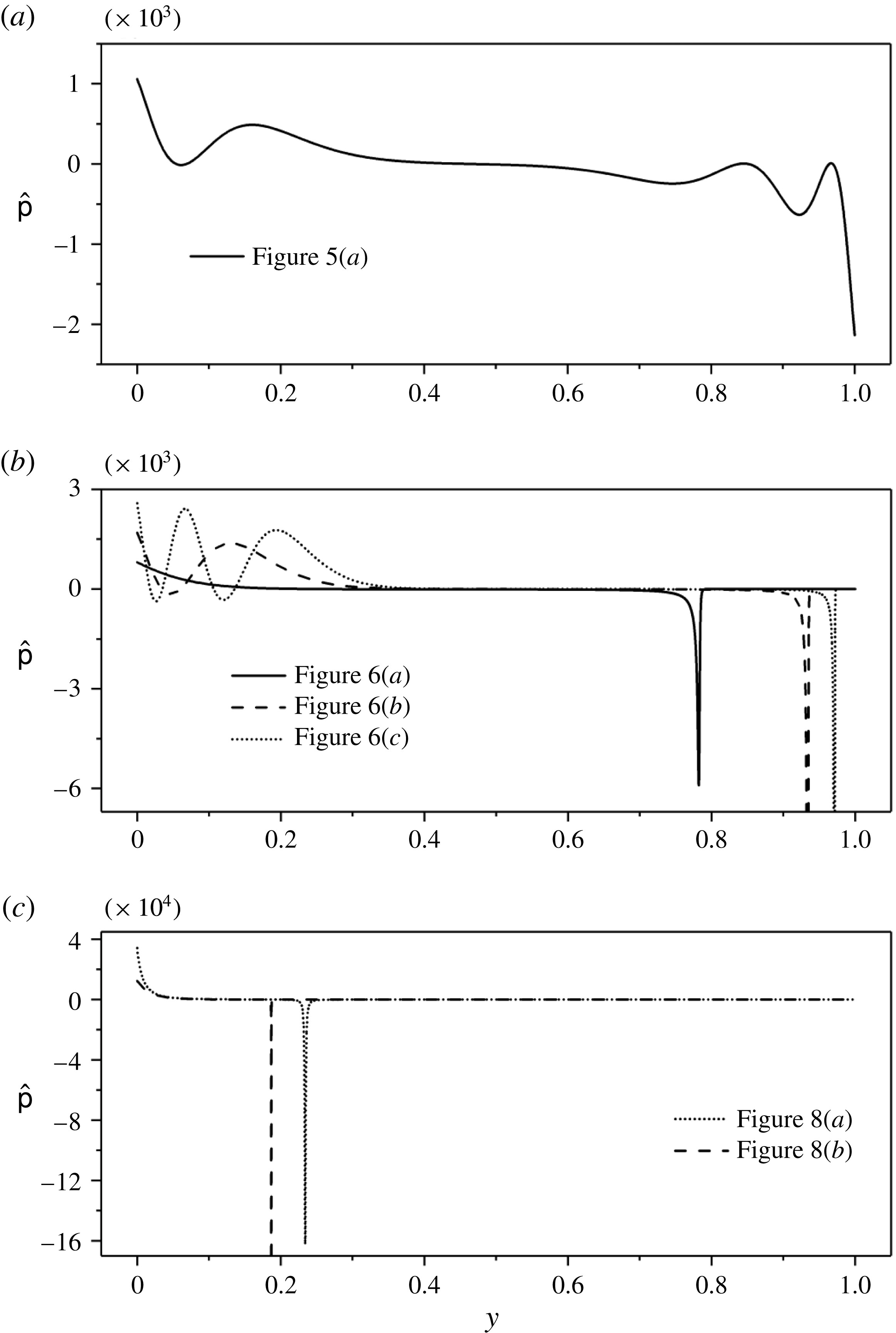
The pseudo-momentum density
 $\hat{\mathsf{p}}$
is plotted against
 $y$
in figure 9(a) for a mode destabilized by the resonant coupling of traditional SRI, corresponding to the eigenfunction of figure 5. As pointed out by Vanneste & Yavneh (Reference Vanneste and Yavneh2007), the IGW
 $n_{\pm }$
basic modes have a
 $\mp$
sign for their pseudo-momentum, whereas the signature of
 $\text{KW}_{\pm }$
depends on
 $\unicode[STIX]{x1D6FA}$
: the
 $\text{KW}_{\pm }$
modes have a
 $\mp$
signature if
 $\unicode[STIX]{x1D6FA}>1/2$
, and a
 $\pm$
one when
 $\unicode[STIX]{x1D6FA}<0$
. The coupled mode in figures 5 and 9(a) consists of an
 $\text{IGW}_{-}$
component that is concentrated near the left wall with positive pseudo-momentum (implying the local mean flow is accelerated in the positive
 $x$
-direction), and an
 $\text{IGW}_{+}$
component confined near the right wall with negative pseudo-momentum (accelerating the local mean flow in the negative
 $x$
-direction). Unstable resonance is achieved when their net contributions are balanced.
The pseudo-momentum density
 $\hat{\mathsf{p}}$
in (5.1) for (a) the resonant SRI mode in figure 5, and (b,c) the
 $\text{KW}_{-}$
and
 $\text{IGW}_{-}$
modes destabilized by their interactions with a baroclinic critical level at
 $y=y_{b+}$
shown in figures 6 and 8. Note that the sharp negative peaks at the baroclinic critical levels have been truncated in (b,c) to help reveal the mode structure.

Figure 9(b,c) shows the density
 $\hat{\mathsf{p}}$
for the
 $\text{KW}_{-}$
and
 $\text{IGW}_{-}$
modes destabilized by their interaction with baroclinic critical levels. The modes have very different distribution of pseudo-momentum:
 $\hat{\mathsf{p}}$
is again locally large and positive near the left wall reflecting the Kelvin wave or internal gravity wave localized there. The net contribution of this wave is balanced by that from a sharp negative peak around the baroclinic critical level.
The pseudo-momentum contribution of the baroclinic critical level can be understood by considering the local behaviour of the solutions in the vicinity of
 $y=y_{b\pm }$
. As outlined in § 2.2,
 $\text{d}\hat{u} /\text{d}y\sim a(y-y_{b\pm })^{-1}$
for the singular Frobenius solution, with
 $a$
a constant. Thus,
 $\hat{\mathsf{p}}\sim O(y-y_{b\pm })^{-2}$
near
 $y=y_{b\pm }$
according to (5.1). An estimate for the contribution of the critical level
 $y_{b\pm }$
therefore follows as
 $$\begin{eqnarray}\displaystyle \mp \frac{2\sqrt{R}k|a|^{2}}{m^{2}(2\unicode[STIX]{x1D6FA}-1)^{2}}\int \frac{\text{d}y}{|y-y_{b\pm }|^{2}}\approx \mp \frac{2\unicode[STIX]{x03C0}\sqrt{R}k|a|^{2}}{m^{2}(2\unicode[STIX]{x1D6FA}-1)^{2}|c_{i}|}, & & \displaystyle\end{eqnarray}$$
which corresponds to a sharply localized acceleration of the mean flow. It is now apparent how the basic modes
 $\text{KW}_{-}$
and
 $\text{IGW}n_{-}$
can become unstable by coupling with the
 $y_{b+}$
critical level (or the
 $\text{KW}_{+}$
and
 $\text{IGW}n_{+}$
by interacting with
 $y_{b-}$
). The signatures of the basic modes and the critical level contributions also rationalize how other types of modal instabilities cannot appear.
6 Concluding remarks
In this paper, we have studied the linear instability of three-dimensional rotating stratified shear flow, with a focus on how baroclinic critical levels impact the strato-rotational instability (SRI). We have found that the baroclinic critical levels destroy the resonance mode interactions between the internal gravity and Kelvin waves that underpin traditional SRI. Instead, these waves can become unstable by interacting directly with one of the critical levels. An immediate consequence is that the instability no longer requires any resonance conditions on the modal wavenumber, but occupies an extensive continuous waveband. The situation is somewhat similar to how the classical critical level can affect the linear instabilities of shear flows in shallow water when there are potential vorticity gradients (Kubokawa Reference Kubokawa1984; Balmforth Reference Balmforth1999).
To establish these results, we combined numerical computations of the linear eigenvalue problem with short-wavelength asymptotics. We further examined the pseudo-momentum of the unstable modes to shed further light on how the mode interactions could lead to instability. This quantity must exactly vanish for unstable modes in the stability problem we have studied, and traditional SRI comes about through the resonant interaction of modes with different signatures of pseudo-momentum. For modes destabilized by their interaction with a baroclinic critical level, on the other hand, a thin layer surrounding this level provides a sharp source of pseudo-momentum to balance that of the mode. In other words, the critical level acts like an emitter of the relevantly signed pseudo-momentum.
A key limitation of the present analysis is the assumption of a linear velocity profile, which is unlikely in any physical setting. Once the background vorticity gradient is not zero, the classical critical layer can directly affect the dynamics of the normal modes, whereas here this position plays a more subtle role (our unstable modes all require classical critical levels within the domain to set the stage for destabilizing interactions). Nevertheless, classical critical levels do not always appear to play a significant role in stratified Taylor–Couette flow (Park & Billant Reference Park and Billant2013). One possible explanation for this is that, for the current flow configuration, the singular point associated with the classical critical level is weaker than that resulting from the baroclinic critical level (as gauged by the singularity of the respective Frobenius solutions).
Previous studies on classical critical levels often proceed beyond inviscid linear theory and incorporate nonlinearity and viscosity in view of the relatively high amplitudes and sharp gradients that develop nearby. Here too there are large velocity gradients inside the thin region around the baroclinic critical level, demanding that both viscosity and nonlinearity are important ingredients in ‘baroclinic critical layer’ theory. We leave such a theory for future work, although we note that it must incorporate the interesting feature that the position of the singular level depends on the streamwise wavenumber. Thus, an interesting nonlinear filter may operate within the associated critical layer which divorces the theory from classical analysis.
Acknowledgement
C.W. is supported by the Four Year Doctoral Fellowship of the University of British Columbia, which is gratefully acknowledged.