1 Introduction
This paper considers two- and three-dimensional flow-mediated transport systems operating in flow regimes characterized by finite, moderate Reynolds numbers (
 $1\leqslant Re\leqslant 100$
). In particular, we explore strategies based on viscous streaming effects (enabled by gentle oscillations) to enhance the ability of an active leading object to transport, trap and manipulate passive trailing ones.
We are motivated by the accelerated pace of development of artificial and biohybrid (Williams et al. Reference Williams, Anand, Rajagopalan and Saif2014; Park et al. Reference Park, Gazzola, Park, Park, Di Santo, Blevins, Lind, Campbell, Dauth and Capulli2016; Ceylan et al. Reference Ceylan, Giltinan, Kozielski and Sitti2017) mini-bots enabled by recent simulation (Gazzola et al. Reference Gazzola, Dudte, McCormick and Mahadevan2018; Pagan-Diaz et al. Reference Pagan-Diaz, Zhang, Grant, Kim, Aydin, Cvetkovic, Ko, Solomon, Hollis and Kong2018) and fabrication advances (Ceylan et al. Reference Ceylan, Giltinan, Kozielski and Sitti2017). This new breed of mini-bots predominantly operates in fluids, and brings within reach a range of novel high-impact applications in medicine and manufacturing (drug delivery and particle transport, chemical mixing and in situ contactless manipulation, among many others). Fluid-mediated interactions can then be leveraged to enhance these capabilities or enable new ones (Ceylan et al. Reference Ceylan, Giltinan, Kozielski and Sitti2017).
In general, flow-mediated interactions play an important role in a number of physical and biological phenomena, from fish schooling (Weihs Reference Weihs1973) and suspension of microorganisms (Ishikawa, Simmonds & Pedley Reference Ishikawa, Simmonds and Pedley2006; Koch & Subramanian Reference Koch and Subramanian2011) to cloud particle sedimentation (Metzger, Nicolas & Guazzelli Reference Metzger, Nicolas and Guazzelli2007) and cluster formation (Voth et al.
Reference Voth, Bigger, Buckley, Losert, Brenner, Stone and Gollub2002). Thus, hydrodynamically coupled systems have been investigated for different flow regimes, including Stokes (
 $Re\rightarrow 0$
; Brady & Bossis Reference Brady and Bossis1988, Lauga & Powers Reference Lauga and Powers2009), Oseen (
 $Re\sim O(1)$
; Subramanian & Koch Reference Subramanian and Koch2008) and inviscid (
 $Re\rightarrow \infty$
; Nair & Kanso Reference Nair and Kanso2007, Alben Reference Alben2009, Tchieu, Crowdy & Leonard Reference Tchieu, Crowdy and Leonard2010, Tchieu, Kanso & Newton Reference Tchieu, Kanso and Newton2012). Moreover, interest in fish schooling also prompted a number of such studies (
 $Re>100$
; Liao et al.
Reference Liao, Beal, Lauder and Triantafyllou2003, Liao Reference Liao2007, Borazjani & Sotiropoulos Reference Borazjani and Sotiropoulos2008, Ristroph & Zhang Reference Ristroph and Zhang2008, Bergmann & Iollo Reference Bergmann and Iollo2011, Boschitsch, Dewey & Smits Reference Boschitsch, Dewey and Smits2014, Gazzola, Hejazialhosseini & Koumoutsakos Reference Gazzola, Hejazialhosseini and Koumoutsakos2014, Gazzola et al.
Reference Gazzola, Tchieu, Alexeev, de Brauer and Koumoutsakos2015) including attempts to bridge viscous and inviscid descriptions (Eldredge Reference Eldredge2010).
There has been, however, little effort in characterizing flow coupling mechanisms in the range
 $1\leqslant Re\leqslant 100$
, typical of the emergent technologies highlighted above (Ceylan et al.
Reference Ceylan, Giltinan, Kozielski and Sitti2017). Yet, in this regime, systems of moving objects exhibit rich dynamics characterized by sharp transitions (Gazzola et al.
Reference Gazzola, Mimeau, Tchieu and Koumoutsakos2012a
; Lieu, House & Schwartz Reference Lieu, House and Schwartz2012; Lin, Liang & Zhao Reference Lin, Liang and Zhao2018), leading to markedly different behaviours (transport versus non-transport, attraction versus repulsion) depending on the ratio between viscous and inertial effects.
Given the sharpness of these transitions, we hypothesize that controlled perturbations or second-order effects such as viscous streaming can be leveraged to shift the boundaries between qualitatively different system responses in a rational, regulated fashion. Viscous streaming arises when a fluid of viscosity
 $\unicode[STIX]{x1D708}$
is driven periodically with frequency
 $\unicode[STIX]{x1D714}$
by a vibrating boundary of characteristic length
 $D$
, and is responsible for the generation of steady flow structures that exhibit large spatial and slow temporal scales (relative to
 $D$
and
 $\unicode[STIX]{x1D714}$
). This phenomenon is well understood, both theoretically and experimentally, in the case of individual vibrating cylinders (Holtsmark et al.
Reference Holtsmark, Johnsen, Sikkeland and Skavlem1954; Stuart Reference Stuart1966; Riley Reference Riley1967; Davidson & Riley Reference Davidson and Riley1972; Riley Reference Riley2001; Lutz, Chen & Schwartz Reference Lutz, Chen and Schwartz2005) and spheres (Lane Reference Lane1955; Riley Reference Riley1966; Chang & Maxey Reference Chang and Maxey1994), and has found application in microfluidic flow control, mixing, sorting and pumping (Liu et al.
Reference Liu, Yang, Pindera, Athavale and Grodzinski2002; Marmottant & Hilgenfeldt Reference Marmottant and Hilgenfeldt2003, Reference Marmottant and Hilgenfeldt2004; Lutz, Chen & Schwartz Reference Lutz, Chen and Schwartz2006; Ahmed et al.
Reference Ahmed, Mao, Juluri and Huang2009; Ryu, Chung & Cho Reference Ryu, Chung and Cho2010; He et al.
Reference He, Bi, Hua, Liu, Wen, Wang, Li, Zhu, Lin and He2011; Tovar, Patel & Lee Reference Tovar, Patel and Lee2011; Wang, Jalikop & Hilgenfeldt Reference Wang, Jalikop and Hilgenfeldt2011; Thameem, Rallabandi & Hilgenfeldt Reference Thameem, Rallabandi and Hilgenfeldt2016). Yet little is known in the case of complex geometries and configurations involving multiple objects (House, Lieu & Schwartz Reference House, Lieu and Schwartz2014; Klotsa et al.
Reference Klotsa, Baldwin, Hill, Bowley and Swift2015; Chong et al.
Reference Chong, Kelly, Smith and Eldredge2016; Rallabandi, Wang & Hilgenfeldt Reference Rallabandi, Wang and Hilgenfeldt2017; Dombrowski et al.
Reference Dombrowski, Jones, Katsikis, Bhalla, Griffith and Klotsa2019).
In this work we characterize the impact of viscous streaming in the context of passive two- and three-dimensional particle transport by capitalizing on our previous work (Gazzola et al. Reference Gazzola, Mimeau, Tchieu and Koumoutsakos2012a ) (figure 1 a), and drawing inspiration from previous studies (Tchieu et al. Reference Tchieu, Crowdy and Leonard2010; Chong et al. Reference Chong, Kelly, Smith and Eldredge2013). We thus consider the simple yet representative setting of figure 1(b), characterized by a larger cylindrical bot (master) propelling at a constant forward speed and oscillating transversely, and a smaller, passive, trailing cargo (slave). By means of this idealized experiment, we investigate the slave’s response, dissect the mechanisms at play and challenge our insights to design master geometries that improve transport.
This work is organized as follows. The set-up is detailed in § 2; numerical method and validation are illustrated in § 3; two-dimensional transport applications, analysis and design are presented in § 4; extension to three dimensions is discussed in § 5; and findings are summarized in § 6.
System set-up: (a) baseline (Gazzola et al. Reference Gazzola, Mimeau, Tchieu and Koumoutsakos2012a ) versus (b) current configuration.

2 Physical framework and streaming definitions
We adopt the set-up of figure 1(a) with master and slave cylinders of diameter
 $D_{m}$
(and radius
 $r_{m}$
) and
 $D_{s}=\frac{1}{4}D_{m}$
, respectively, both immersed in a quiescent fluid. The slave is initially at rest, located at a separation distance
 $0.1D_{m}$
behind the master, which impulsively starts translating horizontally with a constant speed
 $U_{l}$
, spanning
 $1\leqslant Re\leqslant 100$
. We refer to this system set-up as the ‘baseline’ throughout, chosen for its minimal complexity and consistency with prior works (Tchieu et al.
Reference Tchieu, Crowdy and Leonard2010; Gazzola et al.
Reference Gazzola, Mimeau, Tchieu and Koumoutsakos2012a
), thus aiding analysis and comparison. In figure 1(b) we superpose to the linear motion of the master a transverse low-amplitude sinusoidal oscillation defined by
 $y^{m}(t)=y^{m}(0)+\unicode[STIX]{x1D716}r_{m}\sin (\unicode[STIX]{x1D714}t)$
with characteristic velocity
 $U_{o}=\unicode[STIX]{x1D716}\unicode[STIX]{x1D714}r_{m}$
, where
 $\unicode[STIX]{x1D714}$
is the angular frequency and
 $\unicode[STIX]{x1D716}=A/r_{m}=0.1$
is the non-dimensional amplitude (
 $A$
denotes amplitude). Oscillations elicit a viscous streaming response which can exert small but non-negligible forces, when compared against wake forces (see supplementary material, § 4.1, available at https://doi.org/10.1017/jfm.2019.643). We claim that this contribution, when properly directed, can significantly alter transport behaviour in a flow regime characterized by sharp transitions (Gazzola et al.
Reference Gazzola, Mimeau, Tchieu and Koumoutsakos2012a
), through constructive effects between wake and streaming components as hinted at in the literature (Kubo & Kitano Reference Kubo and Kitano1980).
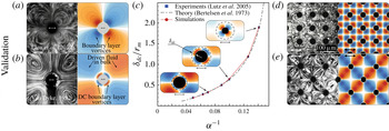
Validation. Comparison of time-averaged streamline pattern in (a) Stokes-like (
 $R_{o}=0.8,R_{s}=0.08$
) and (b) FBL (
 $R_{o}=6.28,R_{s}=0.628$
) regimes against the experiments of Lieu et al. (Reference Lieu, House and Schwartz2012) and Van Dyke (Reference Van Dyke1982), respectively. (c) Normalized DC boundary layer thickness
 $\unicode[STIX]{x1D6FF}_{dc}/r_{m}$
versus
 $\unicode[STIX]{x1D6FC}^{-1}$
(where
 $\unicode[STIX]{x1D6FC}$
denotes the Womersley number
 $r_{m}\sqrt{\unicode[STIX]{x1D714}/\unicode[STIX]{x1D708}}$
) against experiments (Lutz et al.
Reference Lutz, Chen and Schwartz2005) and theory (Bertelsen, Svardal & Tjotta Reference Bertelsen, Svardal and Tjotta1973) in the FBL regime. (d,e) Multiple streaming cylinders comparison against the experiments of House et al. (Reference House, Lieu and Schwartz2014). The two-headed arrows in all panels indicate the direction of oscillations. Simulation details: domain
 $[0,1]^{2}~\text{m}^{2}$
, uniform grid spacing
 $h=1/2048~\text{m}$
, penalization factor
 $\unicode[STIX]{x1D706}=10^{4}$
, mollification length
 $\unicode[STIX]{x1D716}_{moll}=2\sqrt{2}h$
, Lagrangian Courant–Friedrichs–Lewy condition
 $=$
0.01, with viscosity
 $\unicode[STIX]{x1D708}$
and oscillation frequency
 $\unicode[STIX]{x1D714}$
set according to prescribed linear (
 $Re$
) and oscillatory (
 $R_{o}$
) Reynolds numbers. The above values are used throughout the text, unless stated otherwise. We refer to Gazzola et al. (Reference Gazzola, Chatelain, van Rees and Koumoutsakos2011a
) for details of these parameters.

We characterize the linear motion dynamics by
 $Re=U_{l}D_{m}/\unicode[STIX]{x1D708}$
and the oscillatory dynamics by
 $R_{o}=U_{o}r_{m}/\unicode[STIX]{x1D708}$
, where
 $\unicode[STIX]{x1D708}$
is the kinematic viscosity. We further define
 $\unicode[STIX]{x1D701}=R_{o}/Re$
as the non-dimensional quantity that encodes the relative time scales of oscillatory and linear motion. Following Stuart (Reference Stuart1966), we characterize streaming dynamics through the streaming Reynolds number
 $R_{s}=U_{o}^{2}/\unicode[STIX]{x1D708}\unicode[STIX]{x1D714}$
, based on the oscillatory Stokes boundary layer length scale
 $\sqrt{\unicode[STIX]{x1D708}t}=\sqrt{\unicode[STIX]{x1D708}/\unicode[STIX]{x1D714}}$
as
 $t\sim \unicode[STIX]{x1D714}^{-1}$
. While the magnitude of
 $Re$
is an indicator of the flow regime due to linear motion, the magnitude of
 $R_{s}$
similarly characterizes steady streaming structures. Figure 2(a,b) (related to the validation of our numerical solver) illustrates these structures for an oscillating (with no linear translation) cylinder, which consists of distinct regions of clockwise (blue) and counterclockwise (orange) rotating vortical fluid. Figure 2(a) depicts a case with
 $R_{s}\ll 1$
, where viscous effects dominate and the steady streaming flow is Stokes-like, with a single large (infinite for practical purposes) boundary layer that helps match the no-slip condition on the body surface (indicating slow velocity decay; Riley Reference Riley1967). Figure 2(b) is representative of
 $R_{s}$
spanning
 $O(1){-}O(10)$
, where both inertial and viscous effects are comparable. This leads to an ‘outer’ boundary layer (or DC boundary layer) with finite thickness (hence this regime is denoted as the finite outer boundary layer regime or FBL regime). This thickness depends only on the Womersley number
 $\unicode[STIX]{x1D6FC}=r_{m}\sqrt{\unicode[STIX]{x1D714}/\unicode[STIX]{x1D708}}$
(which in the current context represents a scaled oscillatory boundary layer thickness, frequently used as a scaling parameter in the asymptotic expansion of boundary layer equations (Riley Reference Riley1967, Reference Riley2001; Tabakova & Zapryanov Reference Tabakova and Zapryanov1982a
,Reference Tabakova and Zapryanov
b
), as shown in figure 2
c). Over this thickness, the fluid velocity adjusts to match the no-slip condition on the body surface. The DC boundary layer then ‘drives’ the fluid in the bulk (from its outer surface) to set up long-range streaming forces. We note that for fixed
 $\unicode[STIX]{x1D716}$
, as in this work, we can use
 $R_{o}$
alone to characterize streaming flows (as
 $R_{o}=R_{s}/\unicode[STIX]{x1D716}=\unicode[STIX]{x1D716}\unicode[STIX]{x1D6FC}^{2}=\unicode[STIX]{x1D716}\unicode[STIX]{x1D714}r_{m}^{2}/\unicode[STIX]{x1D708}$
).
After introducing viscous streaming in this simple setting, we proceed to study the case of figure 1(b) through numerical simulations via the remeshed vortex method (Gazzola et al. Reference Gazzola, Chatelain, van Rees and Koumoutsakos2011a ), briefly recapped in the following section.
3 Governing equations, numerical method and validation
We consider incompressible viscous flows in an infinite domain (
 $\unicode[STIX]{x1D6F4}$
) in which two density-matched moving rigid bodies are immersed. We denote with
 $\unicode[STIX]{x1D6FA}_{i}$
and
 $\unicode[STIX]{x2202}\unicode[STIX]{x1D6FA}_{i}$
(
 $i=1,2$
) the support and boundaries of the solids. Then the flow is described by the incompressible Navier–Stokes equations (3.1)
 $$\begin{eqnarray}\unicode[STIX]{x1D735}\boldsymbol{\cdot }\boldsymbol{u}=0,\quad \frac{\unicode[STIX]{x2202}\boldsymbol{u}}{\unicode[STIX]{x2202}t}+(\boldsymbol{u}\boldsymbol{\cdot }\unicode[STIX]{x1D735})\boldsymbol{u}=-\frac{1}{\unicode[STIX]{x1D70C}}\unicode[STIX]{x1D735}P+\unicode[STIX]{x1D708}\unicode[STIX]{x1D6FB}^{2}\boldsymbol{u},\quad \boldsymbol{x}\in \unicode[STIX]{x1D6F4}\setminus \unicode[STIX]{x1D6FA}_{i},\end{eqnarray}$$
where
 $\unicode[STIX]{x1D70C}$
is the fluid density. We have the no-slip boundary condition
 $\boldsymbol{u}=\boldsymbol{u}_{i}$
at the body–fluid interface
 $\unicode[STIX]{x2202}\unicode[STIX]{x1D6FA}_{i}$
, where
 $\boldsymbol{u}_{i}$
is the
 $i$
th body velocity. The feedback from the fluid to the
 $i$
th body is described by Newton’s equations of motion
 $m_{i}\ddot{\boldsymbol{x}}_{i}=\boldsymbol{F}_{i}^{H}$
and
 $\unicode[STIX]{x1D644}_{\unicode[STIX]{x1D65E}}\ddot{\unicode[STIX]{x1D73D}_{\boldsymbol{i}}}=\boldsymbol{M}_{i}^{H}$
, where
 $\boldsymbol{x}_{i}$
,
 $\unicode[STIX]{x1D73D}_{\boldsymbol{i}}$
,
 $m_{i}$
,
 $\unicode[STIX]{x1D644}_{\unicode[STIX]{x1D65E}}$
,
 $\boldsymbol{F}_{i}^{H}$
and
 $\boldsymbol{M}_{i}^{H}$
are, respectively, the position of the centre of mass, angular orientation, mass, moment of inertia matrix, hydrodynamic force and moment. This system of equations is solved in velocity–vorticity form by combining remeshed vortex methods with Brinkmann penalization and a projection approach (Gazzola et al.
Reference Gazzola, Chatelain, van Rees and Koumoutsakos2011a
). More details about the method, its computational implementation and run times/resources required for this investigation can be found in the supplementary material, § 1. This method has been extensively validated across a range of biophysical problems, from bluff body flows (including impulsively started cylinders, relevant to this study) to biological swimming (Gazzola et al.
Reference Gazzola, Chatelain, van Rees and Koumoutsakos2011a
; Gazzola, Vasilyev & Koumoutsakos Reference Gazzola, Vasilyev and Koumoutsakos2011b
; Gazzola, van Rees & Koumoutsakos Reference Gazzola, van Rees and Koumoutsakos2012b
; Gazzola et al.
Reference Gazzola, Hejazialhosseini and Koumoutsakos2014).
We now extend this validation to show that the algorithm can also accurately capture second-order streaming dynamics. In figure 2(a,b), we qualitatively compare the streaming structures in the Stokes-like (
 $R_{s}\ll 1$
) and FBL (with
 $R_{s}$
spanning
 $O(1){-}O(10)$
) regimes against corresponding experiments. Figure 2(c) shows the quantitative comparison against prior theory and experiments in the FBL regime, wherein we relate the DC boundary layer thickness (
 $\unicode[STIX]{x1D6FF}_{dc}$
, defined as the offset of the stagnation streamline from the cylinder surface, marked with dashed lines in the insets to figure 2
c) to the inverse Womersley number
 $\unicode[STIX]{x1D6FC}^{-1}=\sqrt{\unicode[STIX]{x1D708}/\unicode[STIX]{x1D714}}/r_{m}$
. We depict streaming structures from multiple oscillating cylinders in figure 2(d,e) to highlight similarity to corresponding experiments. More extensive three-dimensional validation against experiments (Kotas, Yoda & Rogers Reference Kotas, Yoda and Rogers2007, Reference Kotas, Yoda and Rogers2008) can be found in the supplementary material, § 1.5. Overall, through flow visualizations (figure 2
a,b) and boundary layer thickness measurements (figure 2
c), we observe qualitative and quantitative agreement with analytical and experimental studies involving individual and multiple cylinders (figure 2
d,e), thus demonstrating the viability of our numerical approach for this class of problems.
4 Transport in two dimensions
We now assess the impact of streaming on slave transport and quantify it by defining the non-dimensional surface-to-surface separation distance
 $s_{x}(T)/D_{m}$
(figure 1) in the
 $x$
direction. This definition of distance is chosen for consistency with previous studies (Gazzola et al.
Reference Gazzola, Mimeau, Tchieu and Koumoutsakos2012a
), and because of its practical relevance in microfluidic applications in which proximity to objects and clearances are often of concern. A discussion of other possible definitions of distance can be found in the supplementary material, § 3.1.
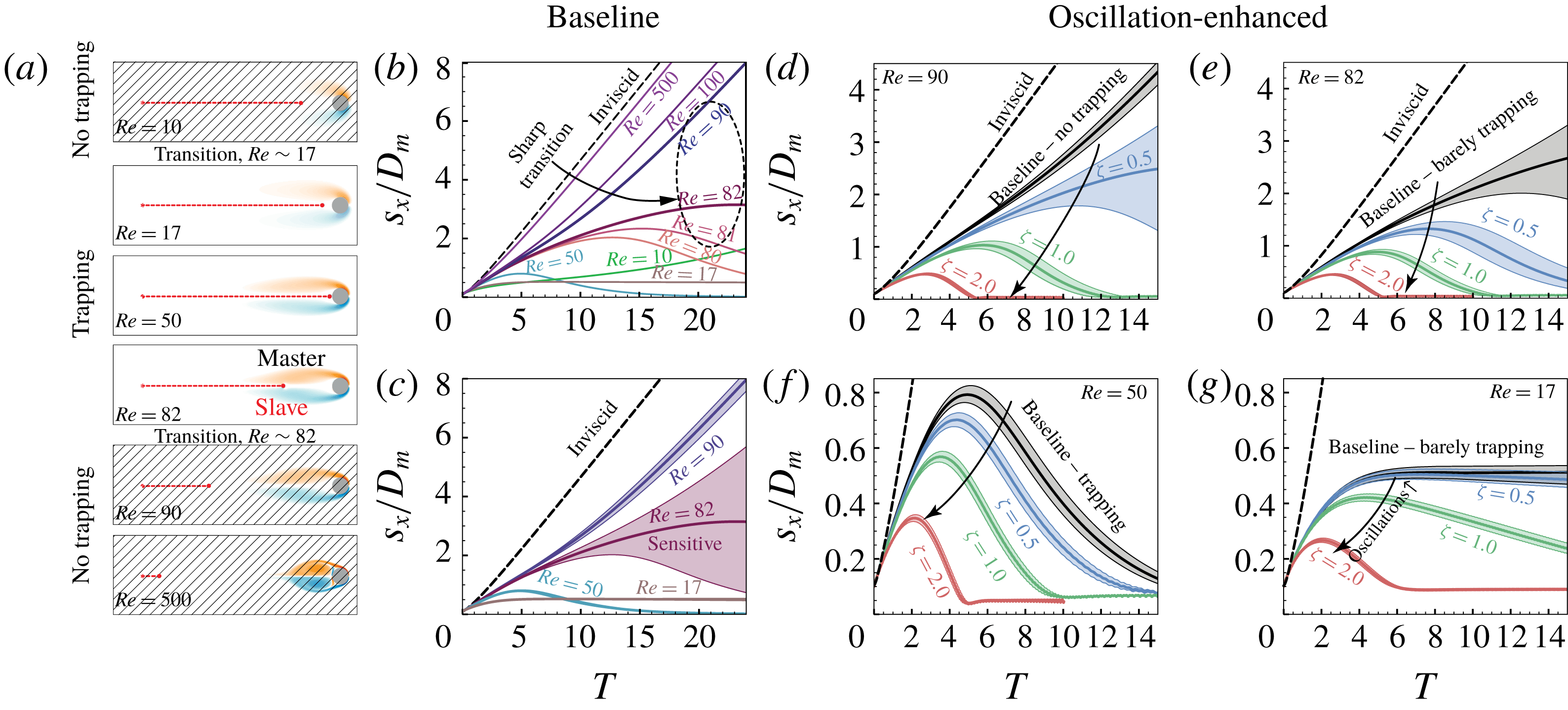
Baseline cases. (a) We observe a clear range of
 $Re$
between which trapping and transport are achievable through linear motion. (b) Plotting
 $s_{x}(t)/D_{m}$
against
 $T=2U_{l}t/D_{m}$
reveals that transport is achieved between
 $Re\approx 17$
and
 $Re\approx 82$
, which then represent transitions between transport and non-transport regimes. At
 $Re\approx 82$
, this transition is sharp (i.e. the system is unstable) and small changes in
 $Re$
lead to very different transport responses. (c) Perturbing the initial slave location and observing
 $s_{x}(t)$
reveals high sensitivity (shaded) of the system around
 $Re\approx 82$
(the top and bottom envelopes of the shaded region represent the characteristics for slaves with a
 $\pm 2\,\%$
perturbation to the initial separation distance). Oscillation-enhanced cases: (d–g) enabling oscillations enhances the ability of the system to transport the slave, across different
 $Re$
.

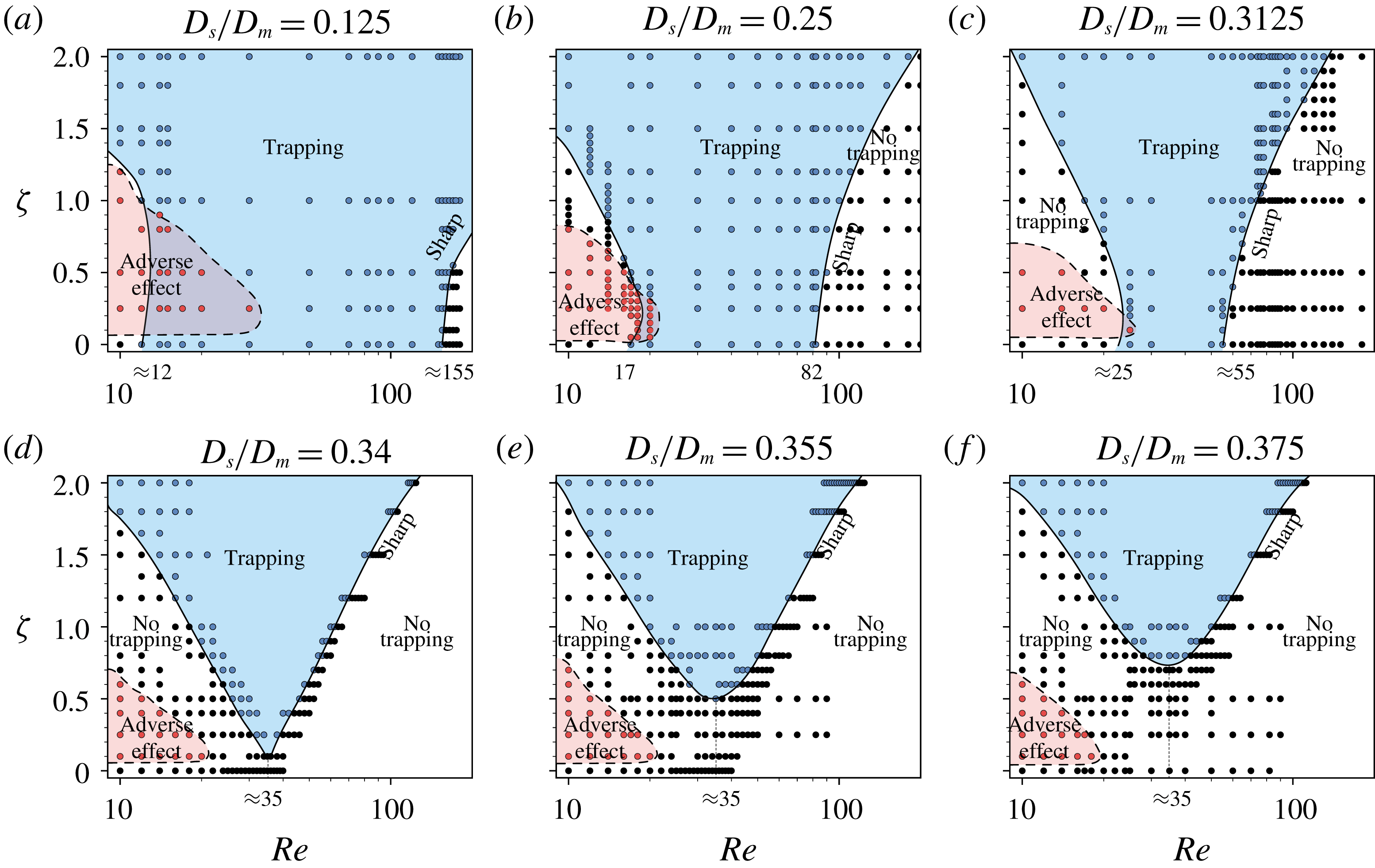
Phase space relating
 $Re$
and
 $\unicode[STIX]{x1D701}$
to the system response (trapping, blue; and no trapping, black) for different
 $D_{s}/D_{m}$
. In some cases at lower
 $Re$
, it is seen that adding oscillations worsens transport behaviour relative to the corresponding baseline. This adverse phase is indicated in red. The transitional
 $Re$
are marked on the bottom of each plot for the baseline (corresponding to
 $\unicode[STIX]{x1D701}=0$
). The sharpness in transitions at higher
 $Re$
is also explicitly indicated. As seen, oscillations enhance inertial particle transport across a range of
 $Re$
and slave inertias
 $D_{s}/D_{m}$
.

4.1 Comparison with baseline
We reproduce the results of the baseline cases of Gazzola et al. (Reference Gazzola, Mimeau, Tchieu and Koumoutsakos2012a
) in figure 3(a) for clarity. As we increase
 $Re$
, we observe two distinct, sharp transitions (at
 $Re\approx 17$
and
 $Re\approx 82$
), between which the slave gets transported (that is, carried along) by the master due to its linear motion (and associated wake) alone. The extent of this transport range is determined by the presence of a maximum in the favourable pressure gradient (consequence of the low-pressure region generated by the wake behind the master) around
 $Re\sim 50$
, and its decay in the lower and higher
 $Re$
limits (supplementary material, § 3.5). The above transport behaviour is then quantified in figure 3(b), where we plot the normalized master–slave separation distance
 $s_{x}/D_{m}$
against the non-dimensional time
 $T=2U_{l}t/D_{m}$
. We note that the non-dimensional time
 $T$
is representative of the number of body lengths (
 $D_{m}$
) travelled by the master. In this plot, a plateauing
 $s_{x}$
or
 $s_{x}\rightarrow 0$
(ergo,
 $\text{d}s_{x}/\text{d}T\leqslant 0$
) indicates transport/trapping and is characteristic of
 $17\lessapprox Re\lessapprox 82$
. Throughout the paper, we will use the terms transport and trapping interchangeably based on the above mathematical condition, the calculation details of which can be found in the supplementary material, § 4.2. For cases with
 $Re\lessapprox 17$
and
 $Re\gtrapprox 82$
,
 $s_{x}$
increases with time indicating that the slave is left behind as the master moves forward and hence it is not transported. At
 $Re\approx 17$
and
 $Re\approx 82$
,
 $s_{x}$
plateaus with increasing
 $T$
, indicating that the slave is transported while maintaining a constant distance from the master (and thus travels with the same speed). These two
 $Re$
then denote the boundaries of transition between trapping and non-trapping regimes. Moreover, at
 $Re\approx 82$
, this transition is sharp, as small changes in
 $Re$
(from
 $80$
to
 $82$
to
 $90$
) lead to large changes in the transport characteristics. Drawing from prior works (Lin et al.
Reference Lin, Liang and Zhao2018), we expect the system to be sensitive to changes in the initial master–slave separation
 $s_{x}(0)$
. We then use this as a proxy to quantify the system sensitivity by perturbing
 $s_{x}(0)/D_{m}$
by
 $\pm 2\,\%$
and observing the resulting transport characteristics. We depict this for a few key
 $Re$
in figure 3(c) for clarity, wherein the shaded regions highlight deviations associated with the perturbation. As expected, the system response is seen to be very sensitive at the transitional
 $Re\approx 82$
, relative to larger and smaller
 $Re$
. We consider this as an opportunity to enhance transport. Indeed a carefully constructed system perturbation can ‘pull’ the system response from the non-transport regime into the sensitive region and make it ‘jump over’, enabling transport. We choose to control the system by perturbing the flow via viscous streaming, by oscillating the master at different levels of intensity
 $\unicode[STIX]{x1D701}=R_{o}/Re$
, and report our observations in figure 3(d–g). For
 $Re=90>82$
(above transition, no baseline transport) shown in figure 3(d), mild oscillations (
 $\unicode[STIX]{x1D701}=0.5$
, blue bands) assist transport and bring the system into the sensitive region. Increasing
 $\unicode[STIX]{x1D701}$
further pushes the system well beyond the transition, enabling (and quickening) slave transport (green and red bands). Figure 3(e–g) shows the oscillation-enabled characteristics for
 $Re=82,50$
and
 $17$
, where we consistently observe a similar behaviour.
We recognize that the system response is dependent not only on initial separation distance
 $s_{x}(0)/D_{m}$
, wake
 $Re$
and oscillation
 $R_{o}$
(encoded in
 $\unicode[STIX]{x1D701}$
) effects, but also on the slave’s inertia captured through
 $D_{s}/D_{m}$
. Therefore, we undertake a parametric investigation to further characterize these dependencies by varying
 $D_{s}/D_{m}$
between 0.125 and 0.375,
 $Re$
between
 $10$
and
 $200$
and
 $\unicode[STIX]{x1D701}$
between
 $0$
and
 $2$
. In figure 4, we report the corresponding
 $Re$
–
 $\unicode[STIX]{x1D701}$
phase spaces in which we indicate whether the slave is trapped or not. From these phase spaces, we observe that oscillations remain beneficial for transport (figure 4
a–f) across a range of
 $Re$
, with smaller slaves more amenable to being trapped. Moreover, as the slave size relative to the master increases, we observe that the trapping phase narrows down and eventually vanishes for large
 $D_{s}/D_{m}$
ratios, consistent with the results of Gazzola et al. (Reference Gazzola, Mimeau, Tchieu and Koumoutsakos2012a
). A minimal scaling analysis provides intuition on the narrowing of the trapping phase. The propulsive force at a given
 $Re$
, obtained by integrating the pressure and viscous shear forces along the slave’s surface, scales approximately linearly with
 $D_{s}$
(since the circumference is
 $\unicode[STIX]{x03C0}D_{s}$
). The inertia of the slave, however, is proportional to its mass (i.e. area) and hence scales as
 $D_{s}^{2}$
. The forces necessary to overcome inertia then grow faster than the forces exerted on the slave’s surface, as a result of which the trapping phase narrows (supplementary material, § 3.4).
Interestingly, in the lower
 $Re$
regime, a new phase appears in which oscillations introduce an adverse effect on transport. This is quantified by the ratio
 $s_{x}/s_{b}$
(at
 $T=10$
), where
 $s_{b}$
is the separation distance of the reference baseline (
 $\unicode[STIX]{x1D701}=0$
) at the corresponding
 $Re$
. Thus, in this region
 $s_{x}/s_{b}>1$
. We add that in some cases, the adverse phase can coexist with the trapping phase (i.e. they are not mutually exclusive). In such cases, the baseline exhibits transport and adding oscillations does not disrupt this behaviour, and the slave simply trails behind the master at larger distances, when compared to the baseline. We defer the explanation of this adverse effect on transport to § 4.2, since the analysis carried out there naturally extends to this. Here, we instead draw attention to the fact that the system retains its inherent sensitivity to
 $Re$
regardless of the slave’s inertia, illustrated by the sharp line separating the trapping/non-trapping phases (supplementary material, § 4.4). We conclude that introducing oscillations, modulated by
 $\unicode[STIX]{x1D701}$
, enhances inertial particle transport across a range of
 $Re$
as well as across different slave inertias. The causal mechanism, be it viscous streaming or other wake–oscillation interactions, is ascertained in the next sections. In the following sections, we will fix
 $D_{s}/D_{m}=0.25$
for consistency with previous works (Tchieu et al.
Reference Tchieu, Crowdy and Leonard2010; Gazzola et al.
Reference Gazzola, Mimeau, Tchieu and Koumoutsakos2012a
), unless specified otherwise.
4.2 Flow analysis at the transport/non-transport boundary
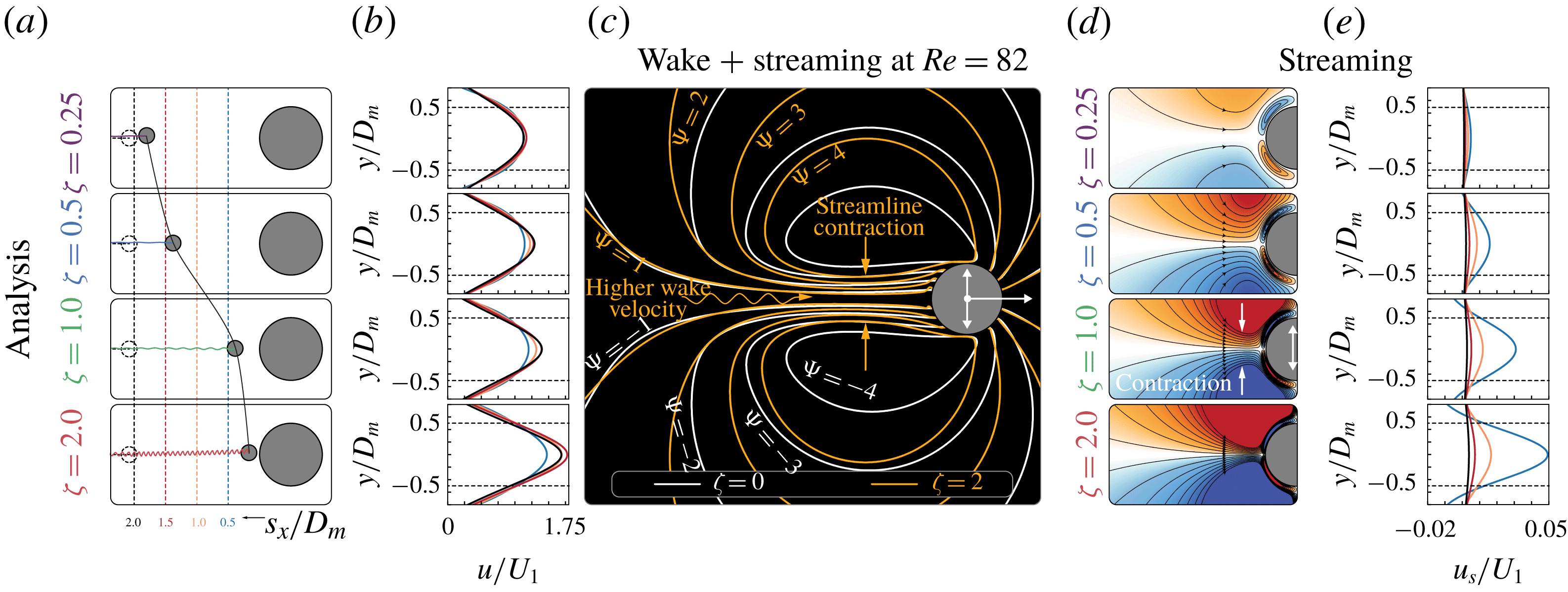
Analysis. Fixing
 $Re=82$
and increasing
 $\unicode[STIX]{x1D701}$
leads to (a) better transport due to flow acceleration in the wake. The cylinders and their trajectories are drawn until
 $T=14$
with the dashed black lines representing the baseline case. (b) Time-averaged velocity profiles (over 20 oscillation cycles) at the marked stations of (a). The observed accelerations are due to streamline contraction in the wake, visualized in (c) for representative cases without (
 $\unicode[STIX]{x1D701}=0$
, white streamlines) and with (
 $\unicode[STIX]{x1D701}=2$
, orange streamlines) streaming. Corresponding streaming-only fields – (d) streamlines and (e) velocities at the same stations as (a,b) – explain the behaviour of (a–c).

Here, we focus on the fluid mechanisms at play by drawing parallels between the system at the transitional
 $Re=82$
(in the case of
 $D_{s}/D_{m}=0.25$
) with different
 $\unicode[STIX]{x1D701}$
and the corresponding pure streaming cases. Figure 5(a) depicts the slave trajectories for increasing
 $\unicode[STIX]{x1D701}$
, highlighting improvement in transport. This is due to a corresponding increase in the wake velocities as seen in figure 5(b), where we plot the time-averaged velocities, at the different stations marked in figure 5(a). The averaged streamlines (streamfunction iso-contours) of figure 5(c) for cases with (
 $\unicode[STIX]{x1D701}=2$
) and without (
 $\unicode[STIX]{x1D701}=0$
) oscillations explain this increase in wake velocity. Adding oscillations to the master displaces the streamlines such that their density is increased behind the master. This localized density increase (or alternatively ‘contraction’ of streamlines) corresponds to an increase in upstream flow velocities (figure 5
b). The degree of this contraction increases with
 $\unicode[STIX]{x1D701}$
. This behaviour is consistent with the corresponding streaming-only patterns of figure 5(d) where larger oscillation intensities increasingly push the outer eddies towards the mid-plane, causing streamline contraction and increasing flow velocities directed towards the master, as further quantified in figure 5(e). We thus identify streamline contraction as the primary cause for transport enhancement, with viscous streaming as driving mechanism.
Finally, this analysis helps explain the appearance of the adverse phase observed in figure 4 at low
 $R_{o}$
(hence at low
 $\unicode[STIX]{x1D701}$
and
 $Re$
, since
 $R_{o}=\unicode[STIX]{x1D701}\cdot Re$
). Indeed, as we lower
 $R_{o}$
, the streaming flow field transitions from the FBL regime to the Stokes-like regime. This, in turn, causes an unfavourable change in the streaming flow direction, which in the Stokes-like regime is directed away from the master. Therefore, the adverse flow reduces the ability of the master to transport the slave. This is further manifested in a corresponding streamline dilatation, instead of contraction. More details and quantitative analysis can be found in the supplementary material, § 4.5.
4.3 Robustness
Given the sensitivity of the system (figure 3
c) to initial horizontal slave separation, it is important to further characterize the spatial robustness of streaming-enhanced transport. We expand our study by initializing (in separate simulations) slaves not only directly behind the master, but all around it (azimuthal positions
 $\unicode[STIX]{x1D703}$
), while retaining the same surface-to-surface distance (
 $0.1D_{m}$
). We choose a representative
 $\unicode[STIX]{x1D701}=0.5$
and vary only
 $Re$
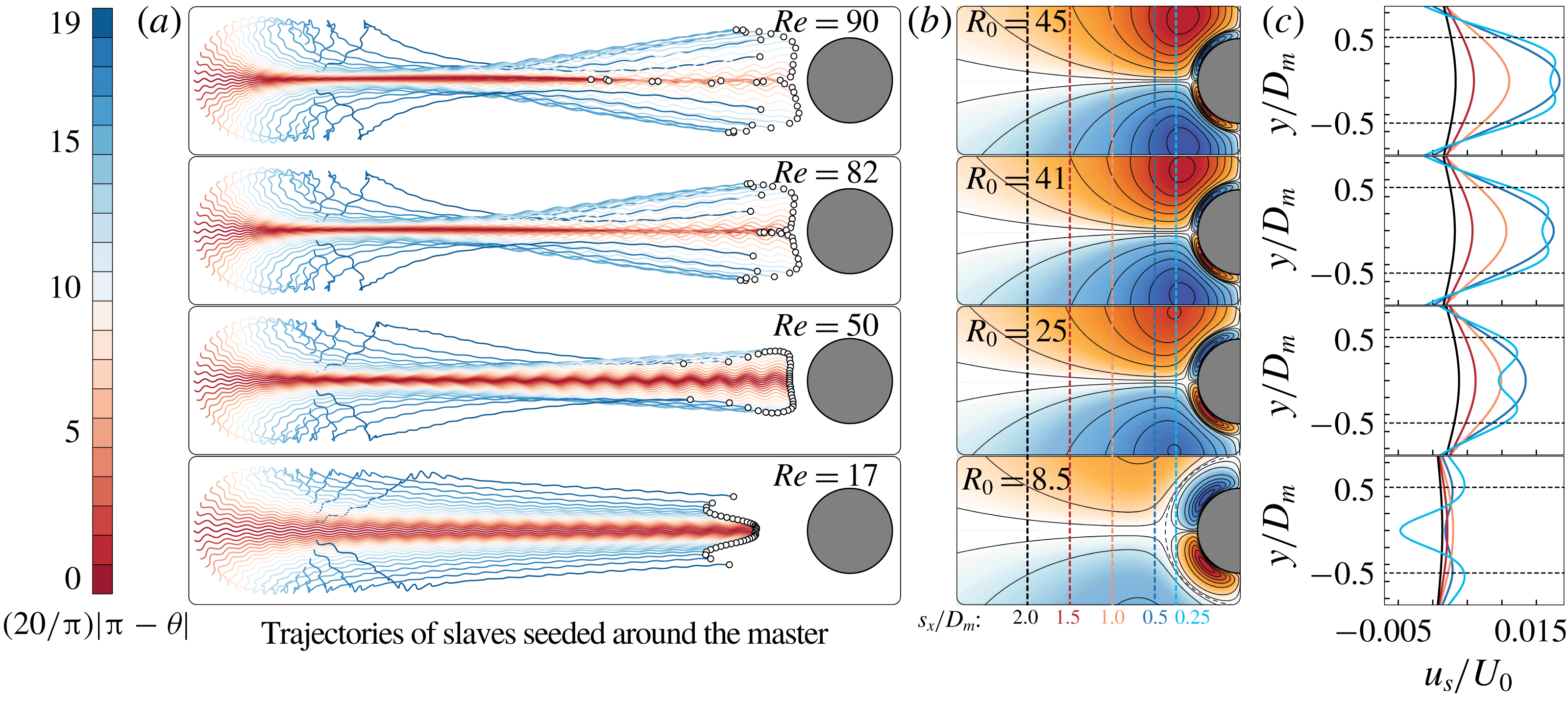
. Figure 6(a) illustrates the slave trajectories up to
 $T=14$
(for consistency) for representative
 $Re$
, coloured by their initial azimuthal positions. We observe that streaming is beneficial when compared to the baseline, even at longer times (
 $2T=28$
), as the number of transported slaves is observed to increase. Only in cases where the baseline already effectively traps (i.e.
 $Re=50$
) does the number of slaves transported not improve (but also is not reduced). Nonetheless, streaming is observed to improve the rate at which slaves approach the master (i.e. their velocities), consistent with figure 3(d–g). More details of the quantification and analyses of robustness to initial radial and azimuthal position perturbations can be found in the supplementary material, §§ 4.6 and 4.7.
Robustness. (a) Seeding slaves (suitably resized for visualization purposes) azimuthally around the master (oscillating with
 $\unicode[STIX]{x1D701}=0.5$
) and plotting their trajectories (until
 $T=14$
) reveal that the streaming-enhanced transport strategy is robust to changes in the initial azimuthal positions. Additionally, streaming is beneficial for transport when compared to the baseline (
 $\unicode[STIX]{x1D701}=0$
) cases across all
 $Re$
investigated, even at longer times (
 $2T=28$
). The supplementary material, § 4.6, contains additional details. Here we report the trajectories only until
 $T=14$
for consistency with the other results. The trajectories shown in (a) can be correlated to (b) the associated pure streaming fields (coloured by streamfunction with the solid lines indicating streamlines). Dashed lines indicate different stations at which we plot (c) streaming-induced velocities. We do not consider slaves in the comparison against pure streaming fields, with the implicit assumption that they do not markedly perturb the flow.

These differences can be understood by analysing the corresponding pure streaming (figure 6
b,c) flow fields. Figure 6(b) shows the time-averaged streamlines, where we also depict the stations at which the corresponding streaming velocities (figure 6
c) are portrayed. At
 $Re=17$
, a thicker DC layer (with reverse flow, blue line in figure 6
c) ‘cushions’ the master and prevents the slaves from attaining close proximity. All the other cases have a DC layer of almost constant thickness, thus leading to qualitative differences, highlighted by slaves closely surrounding the master’s posterior. Comparing
 $Re=50$
and
 $Re=82$
, we notice that in the latter slaves with initial positions
 $|\unicode[STIX]{x03C0}-\unicode[STIX]{x1D703}|\gtrsim 15\unicode[STIX]{x03C0}/20$
(figure 6
a, colourbar) are transported further, due to more favourable upstream velocity profiles. Additionally, slaves almost directly behind the master (with initial positions
 $|\unicode[STIX]{x03C0}-\unicode[STIX]{x1D703}|\lesssim \unicode[STIX]{x03C0}/5$
) are left farther behind for
 $Re=90$
as compared to
 $Re=82$
and
 $Re=50$
. This is explained by the fact that
 $Re=90$
is characterized by a baseline that cannot trap. Mild oscillations (
 $\unicode[STIX]{x1D701}=0.5$
) are then just barely capable of ‘pulling’ the slaves close enough to be trapped and transported, consistent with figure 3(d). We conclude that oscillation-based transport strategy is robust overall (even to radial perturbations, see supplementary material, § 4.7). Moreover the resulting slave trajectories are found to be consistent with streaming-induced velocities, reinforcing the hypothesis that this is indeed the responsible transport enhancement mechanism at play.
4.4 Design
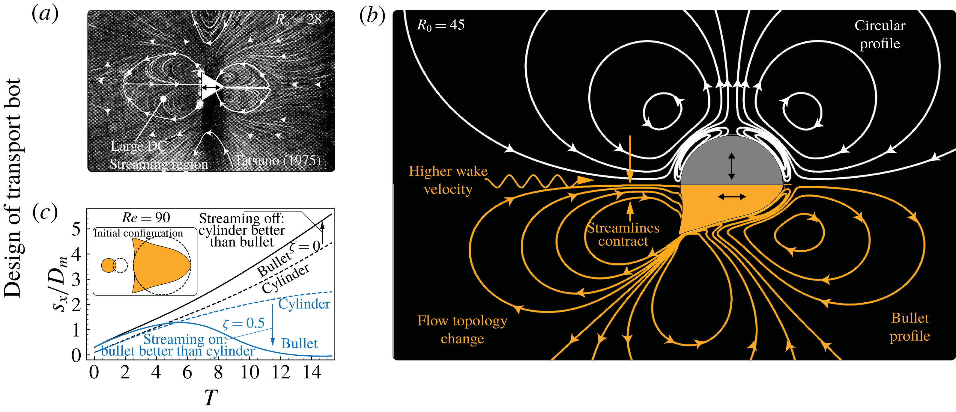
Design. (a) Inspired by streaming from triangles (Tatsuno Reference Tatsuno1975), we design the ‘bullet’ shape of (b) to induce a more favourable streaming field (more streamline contraction at
 $R_{o}=45$
). We note that (b) compares the streamlines of pure streaming fields of the master (top, circular cylinder; bottom, bullet) without linear translation. (c) When the master linearly translates (
 $Re=90$
) and oscillates, the new design exhibits improved transport characteristics owing to its associated streamline contractions. This improvement in transport holds in spite of our initial configuration (inset) that penalizes the bullet by placing the slave further away.

If streaming is indeed the responsible agent for transport enhancement, we should be able to design new geometries that produce more favourable streaming fields that actually translate to improved slave transport once tested in our set-up of figure 1(b). We start by considering streaming only, and draw inspiration from the visual investigation of Tatsuno (Reference Tatsuno1975) on streaming triangles. These are shown to produce a large DC recirculation region (figure 7
a), which can be leveraged to trap and carry along passive cargoes. We then ‘borrow’ two key elements of this geometry – rear high-curvature tips and fore–aft symmetry breaking – to design a master with a ‘bullet’ cross-section (figure 7
c, inset; refer to supplementary material, § 4.8, for shape parametrization). This geometry is an intermediate morph between a circle and a triangle, and is chosen to facilitate the comparison in the case of linear transport (
 $\unicode[STIX]{x1D701}=0$
) between the cylinder and the bullet itself (similar front profile). Due to the break in the fore–aft symmetry of the bullet, the direction of oscillation is important. Here, consistent with the findings of Tatsuno (Reference Tatsuno1975) (figure 7
a), we switch from vertical (transverse) to horizontal (longitudinal) oscillations, so that the large DC recirculation region is located posteriorly, where the slaves are positioned. We note that this is an integral part of our streaming-field design strategy, and as long as
 $Re$
and
 $\unicode[STIX]{x1D701}$
are kept consistent, does not detract from the comparison with vertically oscillating cylinders. In figure 7(b), we show that the longitudinally oscillating bullet constricts the streamlines further than a transversely oscillating circle. This is reflected in its transport characteristics (figure 7
c): while the circular cylinder performs better than the bullet when streaming is not active (no oscillations, pure master linear motion), the bullet outperforms its circular counterpart when streaming is enabled, even for mild oscillation intensities (
 $\unicode[STIX]{x1D701}=0.5$
).
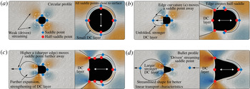
Topology. We study the flow topological response to incremental shape changes (from the (a) circle to the (d) bullet) via line integral convolution of the streaming velocity field at
 $R_{o}=45$
. This reveals a route for the rational design of streaming-based transport devices. The key idea involves introducing rear high-curvature points and fore–aft symmetry breaking to enlarge/strengthen DC layer streaming, the extent of which is indicated by the saddle points and marked by solid black lines. (b,c) Intermediate shapes that illustrate the process.

The reason for the increased streamline contraction above lies in the flow topology change associated with the introduction of multiple curvatures and asymmetry in the master geometry (figure 7 b). To understand how this topological transition occurs, we progressively morph (figure 8) the circular cylinder into the bullet, and track the behaviour of critical points in the flow (these are saddle and half-saddle points (Hunt et al. Reference Hunt, Abell, Peterka and Woo1978), which provide a sparse yet complete representation of the global field (Perry & Chong Reference Perry and Chong1987)). In the context of streaming, saddle points indicate the physical extent of the DC layer, marked by solid black lines in figure 8. Morphing may create, destroy, merge or displace saddle and half-saddle points, which we leverage to manipulate the DC layer. Introducing high rear curvature points to the circle in figure 8(b) creates two new half-saddles, which allow the rear saddle point to move away from the surface, thus ‘unfolding’ the DC layer. The extent of this offset and the corresponding strength of the DC streaming region are related to the magnitude of the tip curvature. This is seen in figure 8(c) where tip curvature increase enlarges the DC layer. Streamlining the master geometry further strengthens the DC layer and gives rise to our final bullet (figure 8 d) design. Thus by manipulating the shape (and the oscillation direction) of the master – which dictates the streaming flow topological response – we can rationally design configurations that improve slave transport.
We conclude this section wherein we have conducted extensive two-dimensional investigations to analyse, understand and design streaming-based transport systems. In the next section, we carry forth these ideas to three dimensions.
5 Transport in three dimensions
Here we investigate how streaming enhancement strategies translate in a three-dimensional transport setting. The use of spheres instead of cylinders does not lead to slave transport, in contrast with two-dimensional results (supplementary material, § 4.9). We then proceed to elongate the master body with an end-to-end length
 $L_{m}$
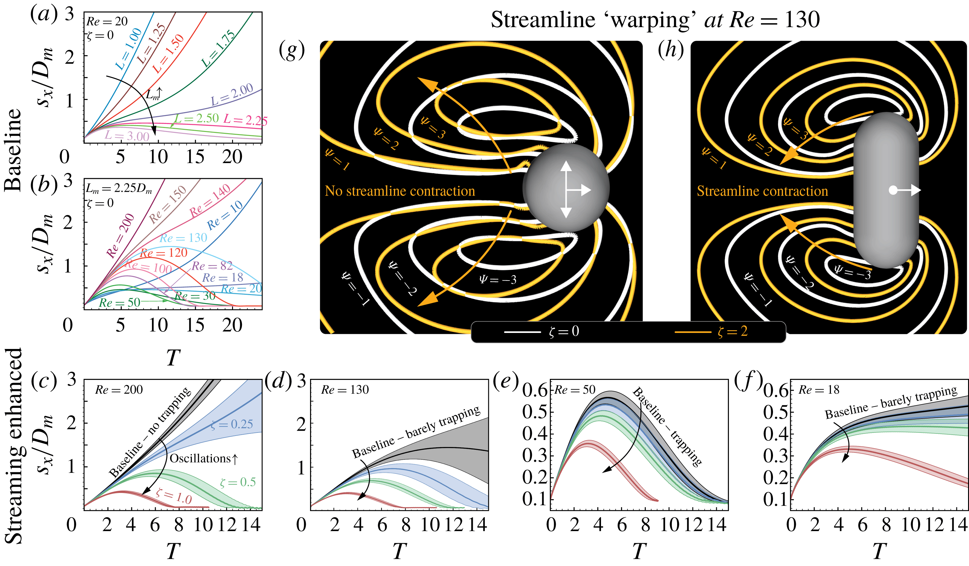
, producing a pill-shaped cylinder with hemispherical ends, striking a compromise between a sphere and a circular cylinder. Figure 9(a) demonstrates the master’s ability to transport/trap the slave at
 $Re=20$
(supplementary material, § 4.9) via linear motion by increasing
 $L_{m}$
. Evaluating the performance of the master with
 $L_{m}=2.25D_{m}$
(sensitive, barely trapping regime) across different
 $Re$
(figure 9
b) reveals two transition regimes (at
 $Re\approx 18$
and
 $Re\approx 130$
), qualitatively consistent with observations in two dimensions.
Baseline. (a) Increasing
 $L_{m}$
suggests that trapping via linear motion is feasible at
 $Re=20$
. (b) Performance of
 $L_{m}=2.25D_{m}$
across different
 $Re$
reveals transport/non-transport transitions at
 $Re\approx 18$
and
 $Re\approx 130$
(barely trapping and sharp transition). Streaming-enhanced. (c–f) Enabling oscillations enhances the ability of the system to trap/transport the slave across different
 $Re$
. Comparing the streamlines for cases without (
 $\unicode[STIX]{x1D701}=0$
) and with (
 $\unicode[STIX]{x1D701}=2$
) oscillation at
 $Re=130$
reveals that streamline contraction does not happen on the (g) oscillation plane but on the (h) plane perpendicular to the oscillation plane.

We again introduce oscillations and perturbations for a few key
 $Re$
(figure 9
c–f) and observe the enhancement in transport capability of the system. We relate this enhancement to the streamline contraction ensuing from streaming. However, contrary to the two-dimensional counterpart, the contraction manifests on the plane perpendicular to the oscillation plane (figure 9
g,h). While the concept of leveraging streaming for transport extends from two to three dimensions, the same contraction mechanism is found to be activated differently. A full three-dimensional characterization is beyond the scope of this study and will be pursued in a follow-up investigation.
6 Conclusions
We have shown that oscillations can be utilized to robustly improve transport in an idealized two-dimensional master–slave setting across
 $1\leqslant Re\leqslant 100$
. The analysis of flow features identifies viscous streaming as the catalyst for this improvement. Leveraging this information, we designed geometries exhibiting more favourable streaming patterns, which resulted in improved slave transport. To that extent, we demonstrated a rational design approach by modifying the classic circular cylinder via the introduction of multiple curvatures and fore–aft symmetry breaking. Moreover, we showed that similar concepts extend to three dimensions even though favourable streaming effects are activated differently.
In conclusion, we have highlighted viscous streaming as a robust mechanism for achieving flow and passive particle control in a regime associated with emerging miniaturized robotic applications, such as, for example, drug delivery. However, despite the potential of viscous streaming in the context of complex, moving geometries, we still understand surprisingly little. What is the role of body shape and curvature in streaming? How can streaming from multiple bodies be effectively used at a collective level? How do three-dimensional effects affect it? While we have presented a rigorous, extensive study in a simplified setting, all these questions remain avenues of future work.
Acknowledgements
The authors acknowledge support by the National Science Foundation under NSF CAREER grant no. CBET-1846752 (M.G.) and by the Blue Waters project (OCI-0725070, ACI-1238993), a joint effort of the University of Illinois at Urbana-Champaign and its National Center for Supercomputing Applications. We thank S. Hilgenfeldt for helpful discussions over the course of this work and W. M. van Rees for technical support on three-dimensional simulations.
Supplementary material
Supplementary material is available at https://doi.org/10.1017/jfm.2019.643.