1 Introduction
Sheared particulate suspensions represent a quasi-unique system where efficient dispersion spontaneously occurs even under low-Reynolds-number flow conditions. For instance, the transfer of heat (Sohn & Chen Reference Sohn and Chen1984; Metzger, Rahli & Yin Reference Metzger, Rahli and Yin2013) or mass (Wang & Keller Reference Wang and Keller1985; Wang et al. Reference Wang, Koch, Yin and Cohen2009; Souzy et al. Reference Souzy, Yin, Villermaux, Abid and Metzger2015) across a suspension of non-Brownian particles is significantly enhanced when the suspension is submitted to a macroscopic shear. This would not happen in a pure Newtonian fluid, where the laminar streamlines remain perpendicular to the scalar (heat or concentration) gradients. In a sheared suspension, the macroscopic stationary imposed shear results at the particle scale in an unstationary flow: particles constantly collide with one another, change streamlines, and thus generate disturbances within the fluid which promote the dispersion of the scalar, prelude to its subsequent mixing. Two mechanisms have been identified to explain the origin of the transfer enhancement. First, the particle translational shear-induced diffusivity, a phenomenon which has been widely investigated over the last decades (Arp & Mason Reference Arp and Mason1976; Eckstein, Bailey & Shapiro Reference Eckstein, Bailey and Shapiro1977; Da Cunha & Hinch Reference Da Cunha and Hinch1996; Breedveld et al. Reference Breedveld, van den Ende, Bosscher, Jongschaap and Mellema2002; Sierou & Brady Reference Sierou and Brady2004; Metzger et al. Reference Metzger, Rahli and Yin2013). Second, the particle rotation, whose impact is particularly important at the boundaries, where particles disrupt the diffusive boundary layer by a ‘rolling-coating’ effect (Souzy et al. Reference Souzy, Yin, Villermaux, Abid and Metzger2015). These studies mainly focused on the rate of transfer across sheared suspensions, which is customarily characterized by an effective diffusion coefficient much larger than the scalar molecular diffusivity.
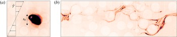
Some dye, initially confined to a small blob in a flowing particulate suspension (a), mixes with the rest of the suspension (b) by diffusing while the blob is stretched in the complex micro-flow generated by the particles.

Another aspect of transport enhancement concerns the mixing properties of the system, namely its ability, starting from a given spatial scalar distribution, to reach homogeneity. Figure 1 shows how a blob of dye with initial size
 $s_{0}$
, diffuses while it is deformed by the complex flow in the interstitial fluid of a suspension. The important question which naturally arises is to understand how this initially segregated system reaches homogeneity, and particularly how long this process takes. By essence, it involves both advection by the flow and molecular diffusion of the scalar. Such a problem has been studied in a wide range of situations involving a single fluid phase such as shear flows (Ranz Reference Ranz1979), vortex flows (Meunier & Villermaux Reference Meunier and Villermaux2003), turbulent jets (Duplat, Innocenti & Villermaux Reference Duplat, Innocenti and Villermaux2010), or flows in porous media (Le Borgne, Dentz & Villermaux Reference Le Borgne, Dentz and Villermaux2015). These studies all underline the crucial importance of the rate at which fluid material lines are elongated by the flow (Villermaux Reference Villermaux2012). The knowledge of these ‘stretching laws’ allows one to estimate the mixing time: the time when the scalar concentration fluctuations start to significantly decay (Batchelor Reference Batchelor1959). For instance, in a simple shear flow with rate
 $\dot{\unicode[STIX]{x1D6FE}}$
, the material lines grow as
 $\dot{\unicode[STIX]{x1D6FE}}t$
. In the limit of large Péclet number
 $Pe=\dot{\unicode[STIX]{x1D6FE}}s_{0}^{2}/D$
, the mixing time for a scalar blob of initial size
 $s_{0}$
is
 $t_{mix}\sim \dot{\unicode[STIX]{x1D6FE}}^{-1}Pe^{1/3}$
, where
 $D$
denotes the molecular diffusivity of the dye. In chaotic flows, where the stretching rate is maintained, the material lines stretch exponentially, as
 $\text{e}^{\dot{\unicode[STIX]{x1D6FE}}t}$
, and
 $t_{mix}\sim \dot{\unicode[STIX]{x1D6FE}}^{-1}\ln Pe$
.
In spite of their crucial importance for mixing issues, stretching laws in particulate suspensions have never been studied experimentally, nor has the general question about the mixing time in such a system. Stretching in particulate suspension has been addressed indirectly using numerical simulations through the measurement of the suspension largest Lyapunov exponent (Dasan et al. Reference Dasan, Ramamohan, Singh and Nott2002; Drazer et al. Reference Drazer, Koplik, Khusid and Acrivos2002; Metzger & Butler Reference Metzger and Butler2012b ; Metzger, Pham & Butler Reference Metzger, Pham and Butler2013). In such a chaotic system, the mean stretching rate of fluid elements can be assimilated to the largest Lyapunov exponent. The reported positive Lyapunov exponents indicate that the stretching laws must be exponential. Stretching has also been explored theoretically with the motivation of understanding the rheology of such systems when the suspending fluid is viscoelastic. It was shown that the expected exponential stretching of the polymers should affect the pressure drop in fixed beds of spheres or fibres (Shaqfeh & Koch Reference Shaqfeh and Koch1992) or the viscosity of freely suspended fibres in a simple shear flow (Harlen & Koch Reference Harlen and Koch1993).
In this paper, we specifically address the question of the stretching kinematics by performing experiments on non-Brownian and spherical particulates suspended in a viscous and Newtonian fluid that is steadily and uniformly sheared. In this limit, the flow kinematics is independent of both the shear rate
 $\dot{\unicode[STIX]{x1D6FE}}$
and the molecular diffusivity. The sole parameter expected to affect the stretching process is the particulate volume fraction
 $\unicode[STIX]{x1D719}$
. We investigate the stretching laws in particulate suspensions varying the volume fraction over a wide range
 $20\,\%\leqslant \unicode[STIX]{x1D719}\leqslant 55\,\%$
, for which collective effects between particles are present but the suspension still flows easily, since it is still far from jamming. After presenting the experimental set-up in § 2, we first compare the evolution of a blob of dye sheared in a pure fluid (without particles) to that of a blob sheared in a suspension (§ 3). This experiment illustrates the complexity of the advection field induced by the presence of the particles. Then, following the Diffusive Strip Method of Meunier & Villermaux (Reference Meunier and Villermaux2010), accurate velocity field measurements of the fluid phase (§ 2.3) are used to determine the stretching laws. Material lines are found to stretch, on average, exponentially with time (§ 4), at a rate which agrees with the largest Lyapunov exponents reported in three-dimensional (3D) Stokesian dynamic simulations (Dasan et al.
Reference Dasan, Ramamohan, Singh and Nott2002; Drazer et al.
Reference Drazer, Koplik, Khusid and Acrivos2002). Beyond the mean, we tackle the complete statistics of stretching, that is to say, the distributions of elongation as a function of strain and particle volume fraction, which are found to converge towards log-normal distributions. In § 5, we present a model, based on a multiplicative stretching process, which explains quantitatively the experimental distributions of the material line elongation and its dependence on
 $\dot{\unicode[STIX]{x1D6FE}}t$
and
 $\unicode[STIX]{x1D719}$
. Finally, the crucial implication of these findings for scalar mixing are developed and discussed in § 6, before we conclude in § 7.
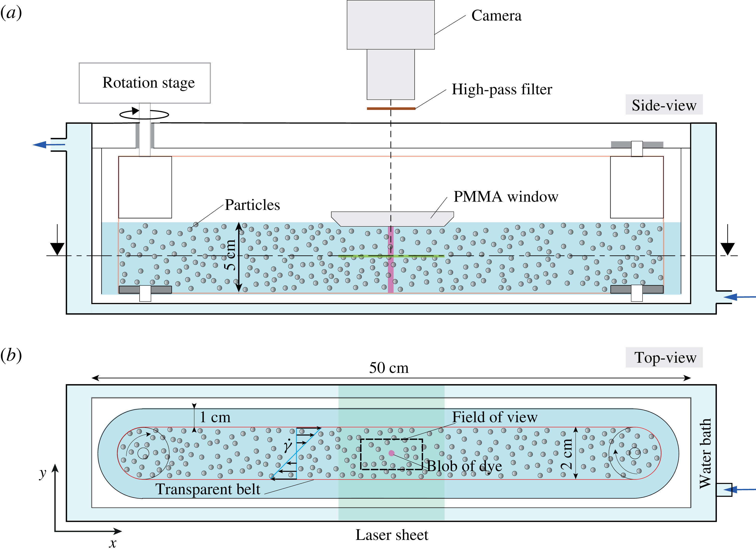
Schematics of the set-up.

2 Experimental set-up
The experimental set-up is shown in figure 2. It aims at steadily and uniformly shearing a viscous particulate suspension, injecting a small blob of dyed fluid, and observing both the flow and the mixing of the dye. The set-up consists of a transparent cell in which a transparent mylar belt is tightly mounted at the top of the cell on two cylinders and at the bottom on two ball bearings. One cylinder is entrained by a rotating stage (M-061.PD from PI Piezo-Nano Positioning) with high angular resolution (
 $3\times 10^{-5}$
rad). The motion of the belt generates in its central region a linear shear flow. The suspension is allowed to flow below the cylinders and a constant spacing between the belt and the inner wall of the cell is maintained all around the cell. This specific design, which is an evolution of that used in Metzger & Butler (Reference Metzger and Butler2012a
), minimizes secondary flows and ensures a velocity profile with constant shear rate within the belt.
2.1 Particles and liquid
The particles and the liquid are carefully chosen to allow the visualization of the dye and of the flow inside the suspension, as well as to ensure a purely viscous flow without buoyancy effects. This requires using a transparent media, matching both the density and the refraction index of the particles, and using a fairly viscous liquid.
To fulfil the above requirements, we use mono-disperse spherical particles (PMMA from Engineering Laboratories Inc.) with density
 $\unicode[STIX]{x1D70C}=1.18~\text{kg}~\text{m}^{-3}$
and diameter
 $d=2~\text{mm}$
, especially chosen for their smooth surface and good transparency. The liquid is a Newtonian mixture of Triton X-100 (77.4 wt.%), zinc chloride (13.4 wt.%) and water (9.2 wt.%) with viscosity
 $\unicode[STIX]{x1D702}=3$
Pa s and having the same density as the particles at room temperature. Its composition is optimized to match both the refractive index and the density of the particles. A small amount of hydrochloric acid (
 ${\approx}$
0.05 wt.%) is added to the solution to prevent the formation of zinc hypochlorite precipitate, thereby significantly improving the optical transparency of the solution. Last, to finely tune the index matching between the particles and the liquid, the temperature of the set-up is adjusted with a water bath surrounding the shear cell.
The solid volume fraction
 $\unicode[STIX]{x1D719}$
of the suspension is varied between 20 % and 55 %. To ensure that inertial effects are negligible, the shear rate
 $\dot{\unicode[STIX]{x1D6FE}}$
is set to typically
 $0.15~\text{s}^{-1}$
, which corresponds to a particulate Reynolds number
 $\unicode[STIX]{x1D70C}\dot{\unicode[STIX]{x1D6FE}}d^{2}/\unicode[STIX]{x1D702}\sim 10^{-4}$
.
2.2 Imaging
The suspension is observed in the flow-gradient plane (
 $xy$
plane): a slice of suspension is illuminated by a laser sheet across the transparent belt and imaged from the top (see figure 2).
The laser sheet is formed by reflecting a laser beam (2 W, 532 nm) on a standard laser-printer mirror (rotating at
 ${\sim}10\,000$
rpm). This technique was found to produce a light sheet with a better spatial homogeneity than that obtained with classical cylindrical or Powell lens techniques. The sheet is collimated and focused to a thickness of
 ${\sim}60\,\unicode[STIX]{x03BC}\text{m}$
with the help of two perpendicular plano-convex lenses. Last, a high-pass filter (590 nm) eliminates direct light reflections. The suspension is imaged with a high-resolution camera (Basler Ace2000-50gm,
 $2048\times 1080~\text{pixel}^{2}$
, 12bit) coupled to a high-quality magnification lens (Sigma APO-Macro-180 mm-F3.5-DG). To avoid the particles distorting the free surface of the suspension through which the visualization is realized, a small Plexiglas window is positioned on the free surface, above the region of interest, which locally ensures a flat interface. The window has a small hole allowing the injection of a blob of dyed fluid with a syringe.
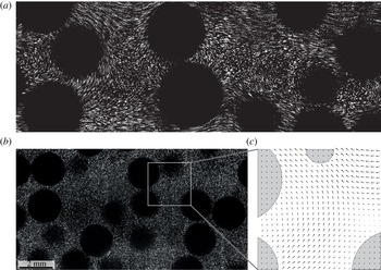
(a) Flow streamlines in the bulk of a suspension. (b) Slice of a sheared suspension illuminated by a laser sheet. The small fluorescent tracers seeding the suspending fluid appear as bright whereas the particle intersections with the laser sheet appear as dark, see also supplementary movie 1 available at https://doi.org/10.1017/ jfm.2016.828. (c) Magnified view of the suspending liquid velocity field obtained from the PIV (the velocity is not computed in the particles).

2.3 Velocity field measurements
The velocity field in the suspending liquid is measured in the plane of the laser sheet (
 $xy$
), at half-distance between the bottom and the free surface (see figure 3), performing particle image velocimetry (PIV), which yields the two-dimensional (2D) velocity field
 $\{u,v\}$
, which does not necessarily verify incompressibility. To perform PIV, the liquid is seeded with small passive fluorescent tracers (
 $3.23\,\unicode[STIX]{x03BC}\text{m}$
PMMA B-particles from MF-Rhodamine) at a very low volume fraction (
 ${\sim}10^{-5}\ll \unicode[STIX]{x1D719}$
). These small and diluted tracers do not affect the flow but allow its visualization and quantification, as shown in figure 3 and movie 1. The large (2 mm) particles of the suspension do not interact with the laser sheet, and appear as black discs. Note that all the particles have the same size; the apparent size differences arise from their different vertical positions relative to the laser sheet plane. The PIV routine is adapted from a Matlab code developed by Meunier & Leweke (Reference Meunier and Leweke2003). Images are captured every 0.1 s, which corresponds to a strain increment of 0.015. To perform PIV, the images are divided into equally spaced and overlapping sub-images with a typical size of
 $d/20$
(32 pixels). The local velocity field is computed by cross-correlating successive sub-images. The presence of a particle in the sub-image is detected with the help of two filters (for the maximum of correlation and for the standard deviation of the sub-images), in which case the corresponding velocity vector is not used (see figure 3
b). For each volume fraction, three independent runs over a strain of 20 are performed. The independence of the measured velocity field on the PIV sub-image size was verified by decreasing the latter to
 ${\sim}d/40$
(16 pixels). Besides increasing the data noise, no significant effect was found on the measured velocities.
2.4 Molecular diffusivity measurements
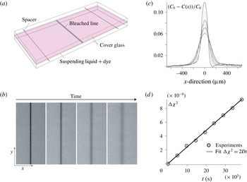
The molecular diffusion coefficient of the dye (rhodamine 6G) is measured by observing the spreading, in the absence of flow, of a slice of liquid depleted in dye. A small Hele-Shaw cell (
 $100~\unicode[STIX]{x03BC}\text{m}$
thick) is filled with dye-doped suspending liquid without particles. A thin slice of liquid is initially depleted in dye by bleaching the dye with a high-power laser sheet across the cell (see figure 4). The depleted slice appears as a dark line having a Gaussian profile which diffuses with the diffusion coefficient of the dye. The spatial variance of the Gaussian profile
 $\unicode[STIX]{x1D712}^{2}$
is measured over one day, and the diffusivity is determined from
 $D=[\unicode[STIX]{x1D712}^{2}(t)-\unicode[STIX]{x1D712}^{2}(0)]/2t\simeq 1.44\times 10^{-13}~\text{m}^{2}~\text{s}^{-1}$
. This value is consistent with that of
 $4.14\times 10^{-10}~\text{m}^{2}~\text{s}^{-1}$
found by Culbertson, Jacobson & Ramsey (Reference Culbertson, Jacobson and Ramsey2002) for the diffusivity of the same dye in water, given that water is 3000 times less viscous than the suspending liquid and that, according to the Einstein–Sutherland law,
 $D\propto 1/\unicode[STIX]{x1D702}$
.
(a) Schematics of the set-up used to measure the molecular diffusivity
 $D$
of the dye (rhodamine 6G), in the suspending liquid (
 $\text{TritonX}+\text{ZnCl}_{2}+\text{H}_{2}\text{O}$
). (b) Diffusive thickening of the bleached line at
 $t=0$
, 4800, 21 600 and 64 800 s (the image width is 5 mm). (c) Concentration profiles at successive times (
 $0~\text{s}<t<64\,800~\text{s}$
). (d) Increase of the spatial variance of the concentration
 $\unicode[STIX]{x1D712}^{2}(t)-\unicode[STIX]{x1D712}^{2}(0)$
versus time. Its fit to
 $2Dt$
yields
 $D=1.44\pm 0.2\times 10^{-13}~\text{m}^{2}~\text{s}^{-1}$
.

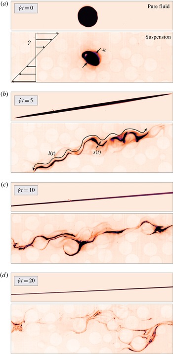
Comparison of the stretching processes of a blob of dye sheared at high Péclet (
 ${\sim}10^{6}$
) and low Reynolds numbers (
 ${\sim}10^{-4}$
), in a pure fluid (top), and in a particulate suspension with volume fraction
 $\unicode[STIX]{x1D719}=35\,\%$
(bottom). The dye appears as dark, and the beads appear as bright, see also supplementary movie 2.

3 General observations
To illustrate the influence of particles on mixing in a shear flow, we first compare the evolution of a blob of dye sheared in a pure fluid (without particles) to that of a blob sheared in the suspension of particles, see supplementary movie 2. A cylindrical blob of dyed fluid is injected, at rest and at
 $t=0$
, in the middle of the shear cell. Initially, the blob has a diameter
 $s_{0}\simeq 2~\text{mm}$
, is aligned with the vorticity direction and is centred on the neutral velocity plane. This results in a macroscopically 2D initial configuration, and ensures that the blob does not drift with the flow but only deforms. Figure 5 shows, for a Péclet number
 $Pe\approx 10^{6}$
, how mixing proceeds in the two sheared media, from the initial segregated state up to a strain
 $\dot{\unicode[STIX]{x1D6FE}}t=20$
. In the pure liquid, the blob of dye stretches homogeneously. Its length increases linearly with time and the blob transverse dimension thus decreases as
 $1/t$
. In the suspension, the situation is markedly different: the fluctuations induced by the particles in the fluid phase strongly impact the evolution of the blob. Several conspicuous features deserve being highlighted: (i) the dispersion and the unfolded length of the blob are significantly enhanced by the particles, (ii) both translational diffusivity (transverse undulations of the blob, see figure 5
b) and rotation (blob winding around particles, see figure 5
c) of the particles contribute to these enhancements, (iii) the blob stretching is highly inhomogeneous: at some locations, its transverse dimension becomes much thinner and at others larger than in the pure fluid case, revealing regions of enhanced stretching and regions of compression, (iv) at large strains (figure 5
d), the blob has separated into several filaments, which means that some regions of the blob have already mixed, while in the pure liquid (without particles) mixing has not occurred yet, (v) in some regions, the blob evolves into bundles composed of several nearly overlapping filaments (Duplat & Villermaux Reference Duplat and Villermaux2008). This suggests an underlying stretching/folding mechanism similar to the well-known baker’s transform (Ottino Reference Ottino1989).
The above features are generic to the flow of a viscous suspension at large Péclet number. Since inertial effects are negligible, these features are independent of the rate
 $\dot{\unicode[STIX]{x1D6FE}}$
at which the suspension is sheared. Similarly, the value of the Péclet number does not influence the general stretching pattern of the blob, but only prescribes the strain
 $\dot{\unicode[STIX]{x1D6FE}}t$
at which diffusion starts to becomes effective.
This direct comparison clearly illustrates how the liquid velocity fluctuations generated by the particles dramatically accelerate the blob deformation and dispersion. This acceleration is apparent here from the beginning of the shear, because the blob size
 $s_{0}$
is similar to the particle size
 $d$
. It is, however, crucial to realize that the strain at which this acceleration establishes is expected to depend on the ratio
 $s_{0}/d$
. If the initial size of the blob
 $s_{0}$
is larger than
 $d$
, the blob is essentially not stretched by the particle fluctuation motions. It is thus essentially stretched by the linear macroscopic shear until the blob transverse size has thinned down to
 $d$
, after a typical strain
 $s_{0}/d$
. From that strain on, the particulate fluctuations are expected to contribute directly to the blob stretching.
In stirred flows, such as the case considered here, mixing results from the coupling between advection and molecular diffusion. In the experiment described above, the blob of dye is stretched by the local velocity field: the blob is stretched along its own longitudinal direction and conversely compressed along its transverse direction. The blob thus evolves towards a topology constituted of sheets, or filaments (Ottino Reference Ottino1989; Buch & Dahm Reference Buch and Dahm1996). Conversely to the effect of advection, molecular diffusion tends to broaden the filaments. This diffusive broadening will at some point counter-balance the rate of compression of the blob caused by the advection. As we already mentioned, this naturally sets a time scale called the mixing time,
 $t_{mix}$
, beyond which the concentration levels drop significantly. The mixing time, a key element to understand the overall mixing process, can be estimated from the sole knowledge of the dye molecular diffusion coefficient and from the history of the transverse dimension of the blob. If one assumes that the flow is two-dimensional (this assumption is discussed in § 5.3), incompressibility and mass conservation relate at any time the transverse size of the blob to its length
 $l$
, through
 $s_{0}l_{0}=s(t)l(t)$
. The mixing time can therefore be estimated from the characterization of the evolution of
 $l(t)$
. Our goal in the following is thus to determine the so-called ‘stretching laws’, i.e. the time dependence of
 $l$
in sheared particulate suspensions.
4 Experimental stretching laws
Our first attempt to measure the unfolded length of the blob
 $l(t)$
was naturally to perform direct image analysis on images such as those shown in figure 5. However, the intrinsic dispersion process rapidly distorts the blob into bundles of very close (sometimes merging) filaments, which renders image analysis ineffective above strains of typically 5.
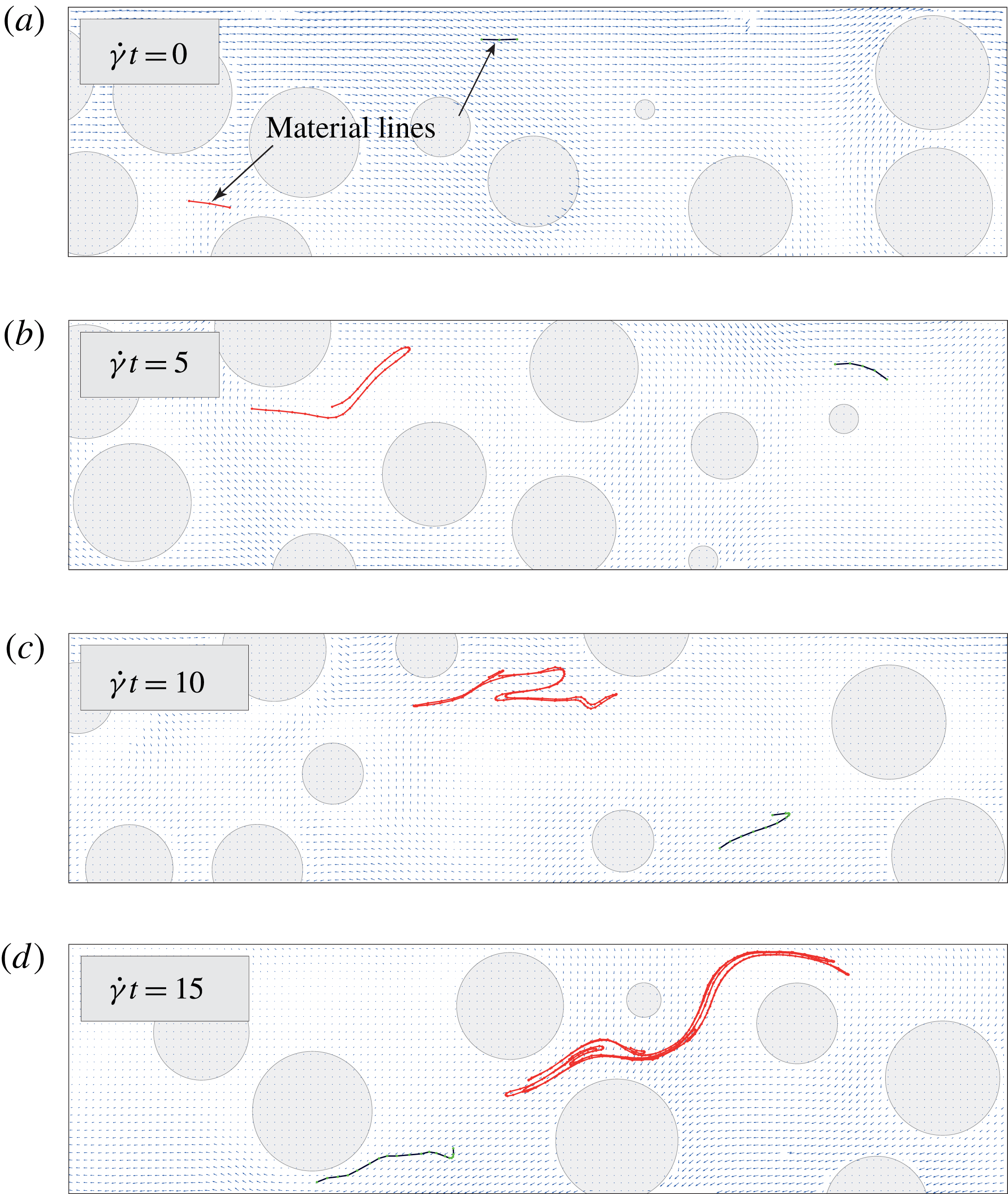
Example of stretching for two material lines numerically advected using the experimental fluid velocity field, see also supplementary movie 3.

To overcome these limitations, we adopted a different approach inspired from the Diffusive Strip Method. This method happens to be a very powerful experimental tool allowing the determination of the stretching laws over unlimited strains. The key idea is to use the experimental fluid velocity field to numerically advect passive material lines representing portions of the blob. The lines are initially composed of three passive tracers, separated by a distance
 $d/20$
, which discretize a fluid material line. The lines are randomly located in the 2D velocity field with a random orientation (see figure 6
a). Each tracer with coordinate
 $\boldsymbol{x}$
is advected independently from each other according to the local fluid velocity
 $\boldsymbol{v}(\boldsymbol{x})$
(obtained by linear interpolation of the instantaneous PIV velocity field) as
 $\boldsymbol{x}(t+\unicode[STIX]{x0394}t)=\boldsymbol{x}(t)+\boldsymbol{v}(\boldsymbol{x})\unicode[STIX]{x0394}t$
, where
 $\unicode[STIX]{x0394}t$
is the time between consecutive measurements of the velocity field. As a material line is advected, it is refined by adding more tracers when its length increases or when its local curvature becomes too large (see Meunier & Villermaux (Reference Meunier and Villermaux2010) for a detailed description of the refinement procedure).
Figure 6 shows the evolution of two material lines up to a strain of 15, see also movie 3. The red line successively stretches and folds very similarly to what is observed in the blob experiments (figure 5). Interestingly, the blue line behaves very differently. Although it sustains the same macroscopic strain as the red one, it experiences a much softer stretching only because it started from a different initial location. These different stretching histories reveal the stochastic nature of the stretching induced within particulate suspensions. The stretching laws therefore have to be sought in a statistical sense by repeating the advection procedure over a large number of independent material lines. However, as the material lines lengthen, they may reach the boundaries of the measured velocity field, which limits the maximum strain that can practically be investigated (typically
 $\dot{\unicode[STIX]{x1D6FE}}t<10$
). This problem is easily circumvented by realizing that, as long as the stretching laws are concerned, the object of interest is not the material line as a whole but rather the small segments which compose this line and which all stretch differently from each other. We thus perform a new set of calculations focusing on segments: (i) initial segments (composed of two tracers) with length
 $d/20$
are positioned and oriented randomly in the flow, (ii) each time the length of a segment doubles, it is split in two individual segments that are subsequently advected independently, (iii) if a segment reaches the boundary of the velocity field, it is re-injected near the centre of the velocity field, (iv) when a segment overlaps with a particle, where the velocity field is undefined (as can happen due to the finite time
 $\unicode[STIX]{x0394}t$
), it is frozen until the particle has moved away. Owing to these rules, virtually unlimited strains can be considered, and the stretching histories of each segment that have been created over this strain can be determined. We define the elongation of these segments as the ratio
 $$\begin{eqnarray}\unicode[STIX]{x1D70C}(t)\equiv \unicode[STIX]{x1D6FF}l(t)/\unicode[STIX]{x1D6FF}l_{0}\end{eqnarray}$$
of their current length
 $\unicode[STIX]{x1D6FF}l(t)$
to their initial length
 $\unicode[STIX]{x1D6FF}l_{0}$
, where
 $\unicode[STIX]{x1D6FF}l_{0}=(d/20)/2^{n}$
, with
 $n$
the number of times the sub-segment was split in two. Note that to compute the distributions of elongations we present below, the contribution of each segment is weighted by its initial length. Note also that times for which a segment is frozen are not considered. The distribution of elongations at time
 $t$
therefore represents the portion of the blob that has reached a given elongation after being advected for a duration
 $t$
. It was built from the stretching histories of 25 000 segments advected over three independent experimental velocity fields, each of them recorded for a total strain of 20 (typically 4000 images).
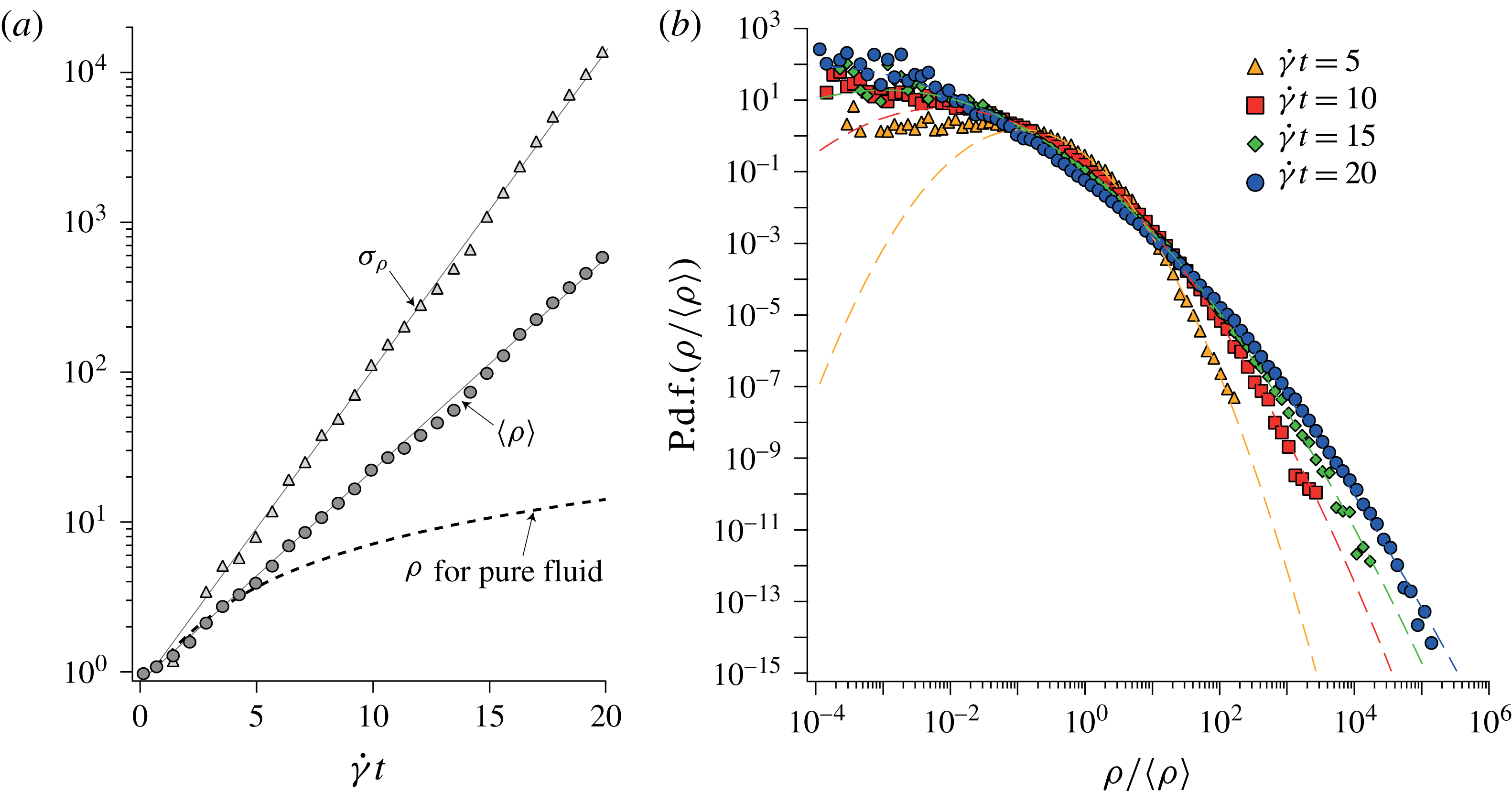
Stretching laws measured for a suspension with volume fraction
 $\unicode[STIX]{x1D719}=35\,\%$
. (a) Mean value
 $\langle \unicode[STIX]{x1D70C}\rangle$
and standard deviation
 $\unicode[STIX]{x1D70E}_{\unicode[STIX]{x1D70C}}=\sqrt{\langle \unicode[STIX]{x1D70C}^{2}\rangle -\langle \unicode[STIX]{x1D70C}\rangle ^{2}}$
of the distribution of elongations versus macroscopic strain in a semilogarithmic representation. The dashed line corresponds to the mean elongation in a pure fluid
 $\unicode[STIX]{x1D70C}_{lin}(t)=\sqrt{1+\dot{\unicode[STIX]{x1D6FE}}^{2}t^{2}/2}$
. (b) Distribution of the normalized elongations
 $\unicode[STIX]{x1D70C}/\langle \unicode[STIX]{x1D70C}\rangle$
at different strains. The dashed curves are log-normal distributions built from the mean value
 $\langle \unicode[STIX]{x1D70C}\rangle$
and standard deviation
 $\unicode[STIX]{x1D70E}_{\unicode[STIX]{x1D70C}}$
of the experimental elongation distributions.

Figure 7 shows the experimental stretching laws obtained for a suspension with
 $\unicode[STIX]{x1D719}=35\,\%$
, which is generic to the volume fraction range 20 %–55 % investigated. It presents the mean value
 $\langle \unicode[STIX]{x1D70C}\rangle$
and the standard deviation
 $\unicode[STIX]{x1D70E}_{\unicode[STIX]{x1D70C}}\equiv \sqrt{\langle \unicode[STIX]{x1D70C}^{2}\rangle -\langle \unicode[STIX]{x1D70C}\rangle ^{2}}$
of the elongation for strains up to 20. At
 $\dot{\unicode[STIX]{x1D6FE}}t=20$
, the segments have on average lengthened by typically
 $10^{3}$
, which is approximately one hundred times larger than in the case of a pure liquid. The striking result is that the presence of particles in a shear flow changes the very nature of the stretching laws from linear to exponential. Indeed, the elongation of material lines in a simple shear (without particles) follows
 $$\begin{eqnarray}\unicode[STIX]{x1D70C}_{lin}(\unicode[STIX]{x1D703},t)=\sqrt{1+2\cos \unicode[STIX]{x1D703}\sin \unicode[STIX]{x1D703}\dot{\unicode[STIX]{x1D6FE}}t+\sin ^{2}\unicode[STIX]{x1D703}\dot{\unicode[STIX]{x1D6FE}}^{2}t^{2}},\end{eqnarray}$$
where
 $\unicode[STIX]{x1D703}$
denotes the angle between the line initial orientation and the flow direction. On averaging
 $\unicode[STIX]{x1D70C}_{lin}^{2}(\unicode[STIX]{x1D703},t)$
over all possible orientations, we obtain
 $$\begin{eqnarray}\unicode[STIX]{x1D70C}_{lin}(t)=\sqrt{1+\dot{\unicode[STIX]{x1D6FE}}^{2}t^{2}/2},\end{eqnarray}$$
which is only of order 10 for a strain of 20, and increases linearly with time for large strains. Equation (4.3) is plotted in figure 7 to illustrate the contrast with the elongations actually measured in particulate suspensions: the mean elongation in suspensions is different both in magnitude and in law.
Moreover, by contrast with the pure fluid case, the stretching variability of individual material lines is very broad, as evidenced by the exponential growth of the standard deviation
 $\unicode[STIX]{x1D70E}_{p}$
. These results corroborate the preliminary blob experimental visualizations where, in the suspension, many filaments having very different transverse thickness can be observed while the pure fluid case solely exhibits one uniform thickness (figure 5
d). More precisely, figure 7(b) shows the distributions of the relative elongations
 $P(\unicode[STIX]{x1D70C}/\langle \unicode[STIX]{x1D70C}\rangle )$
at successive strains. The distribution of elongations broadens rapidly such that, at a strain
 $\dot{\unicode[STIX]{x1D6FE}}t=20$
, it spans more than eight decades. At that strain, the right tail of the distribution contains segments elongated
 $10^{4}$
times relative to the average
 $\langle \unicode[STIX]{x1D70C}\rangle$
, which corresponds to an absolute elongation of
 $\unicode[STIX]{x1D70C}\sim 10^{7}$
, in stark contrast with the uniform average elongation of 10 obtained in a simple shear. As figure 7(b) shows, these distributions are found to be well fitted by log-normal distributions (shown as dashed lines). Note that the apparent absence of data on the left-hand side of the distributions is fully consistent with log-normal distributions. Indeed, for broad distributions, the statistical weight of the left-hand side of the distribution vanishes. Our data thus fully resolve the meaningful part of the distribution.
The advective strip method presented above was repeated with velocity fields measured in suspensions with different volume fractions
 $\unicode[STIX]{x1D719}$
ranging from 20 % to 55 %. The same trends as those detailed for
 $\unicode[STIX]{x1D719}=35\,\%$
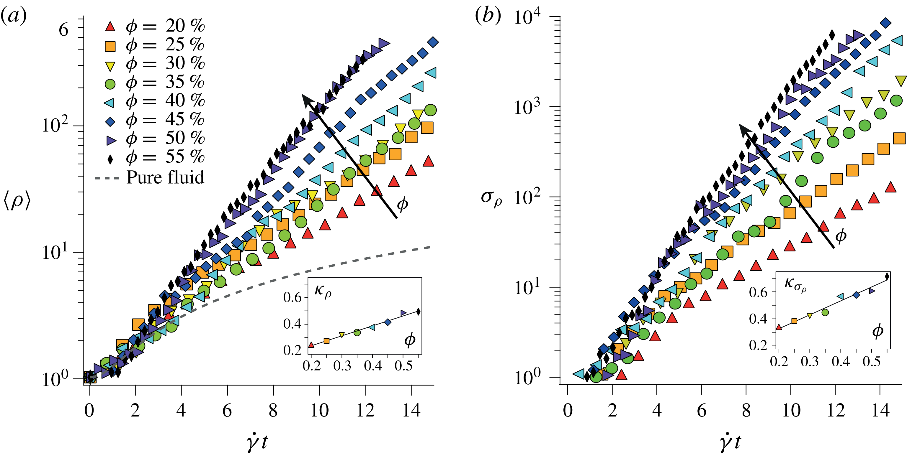
are systematically observed. As shown in figure 8, it is moreover found that larger particulate volume fractions increase both the growth rate of the average elongation
 $\langle \unicode[STIX]{x1D70C}\rangle$
and that of the standard deviation
 $\unicode[STIX]{x1D70E}_{\unicode[STIX]{x1D70C}}$
. This indicates that a larger volume fraction results in larger fluid disturbances which, in turn, induce a faster and more random elongation of the fluid material lines. Fitting these curves with exponential growths in strain
 $\text{e}^{\unicode[STIX]{x1D705}\dot{\unicode[STIX]{x1D6FE}}t}$
yields for
 $\langle \unicode[STIX]{x1D70C}\rangle$
,
 $\unicode[STIX]{x1D705}_{\unicode[STIX]{x1D70C}}=0.09+0.74\,\unicode[STIX]{x1D719}$
, and for
 $\unicode[STIX]{x1D70E}_{\unicode[STIX]{x1D70C}}$
,
 $\unicode[STIX]{x1D705}_{\unicode[STIX]{x1D70E}_{\unicode[STIX]{x1D70C}}}=0.12+1.03\,\unicode[STIX]{x1D719}$
. In the range of volume fraction investigated, the growth rates are found to increase linearly with
 $\unicode[STIX]{x1D719}$
. No measurements could be performed above 55 %, as the large normal stress built in the suspension starts to deform the belt.
To summarize, by kinematically advecting passive segments using the experimental velocity fields of the fluid phase, we measured the elongation of fluid material lines in sheared particulate suspensions. Two important features characterize these elongations: (i) the mean and the standard deviation grow exponentially, (ii) the distribution converges to a log-normal. In the following, using two measurable properties of the fluid velocity field, namely the local shear rate distribution and the Lagrangian correlation time, we present a mechanism accounting for these observations.
Mean elongation
 $\langle \unicode[STIX]{x1D70C}\rangle$
(a) and standard deviation
 $\unicode[STIX]{x1D70E}_{\unicode[STIX]{x1D70C}}$
(b) versus strain for increasing volume fractions ranging from 20 % to 55 %. Insets: growth rate
 $\unicode[STIX]{x1D705}$
of the exponential fit
 $\text{e}^{\unicode[STIX]{x1D705}\dot{\unicode[STIX]{x1D6FE}}t}$
to the main curves, as a function of
 $\unicode[STIX]{x1D719}$
. The lines show
 $\unicode[STIX]{x1D705}_{\unicode[STIX]{x1D70C}}=0.09+0.74\unicode[STIX]{x1D719}$
(a), and
 $\unicode[STIX]{x1D705}_{\unicode[STIX]{x1D70E}_{\unicode[STIX]{x1D70C}}}=0.12+1.03\unicode[STIX]{x1D719}$
(b).

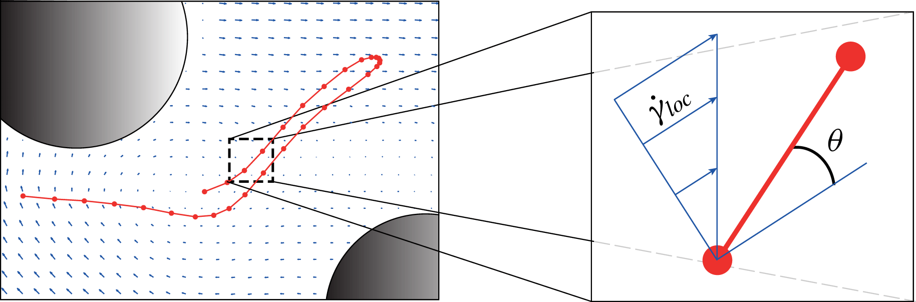
Each segment composing a fluid material line is locally stretched by a simple shear
 $\dot{\unicode[STIX]{x1D6FE}}_{loc}$
which is oriented with a random angle
 $\unicode[STIX]{x1D703}$
with respect to the segment.

5 Origin of the stretching laws
5.1 Principle
We consider the elementary component of a fluid material line: the segment, see figure 9. At that scale, much smaller than the particle size, the local shear
 $\dot{\unicode[STIX]{x1D6FE}}_{loc}$
is uniform. Considering the broad distribution of the segment orientations, we assume that the local shear rate has a random orientation with respect to the segment. Therefore, as long as the local shear rate
 $\dot{\unicode[STIX]{x1D6FE}}_{loc}$
persists, the average elongation of the segment is (see (4.3))
 $$\begin{eqnarray}\unicode[STIX]{x1D70C}=\sqrt{1+\dot{\unicode[STIX]{x1D6FE}}_{loc}^{2}t^{2}/2}.\end{eqnarray}$$
Note that an individual segment can be stretched or compressed depending on whether it is located in a diverging or compressive region of the flow, respectively. However, once averaged over all possible orientations, the segment net elongation is strictly larger than unity. Two questions then naturally emerge: what are the local shear rates? and how long do these shear rates persist? In the following two sections, we address these questions by providing information about the local shear rates and the Lagrangian correlation time of the velocity field.
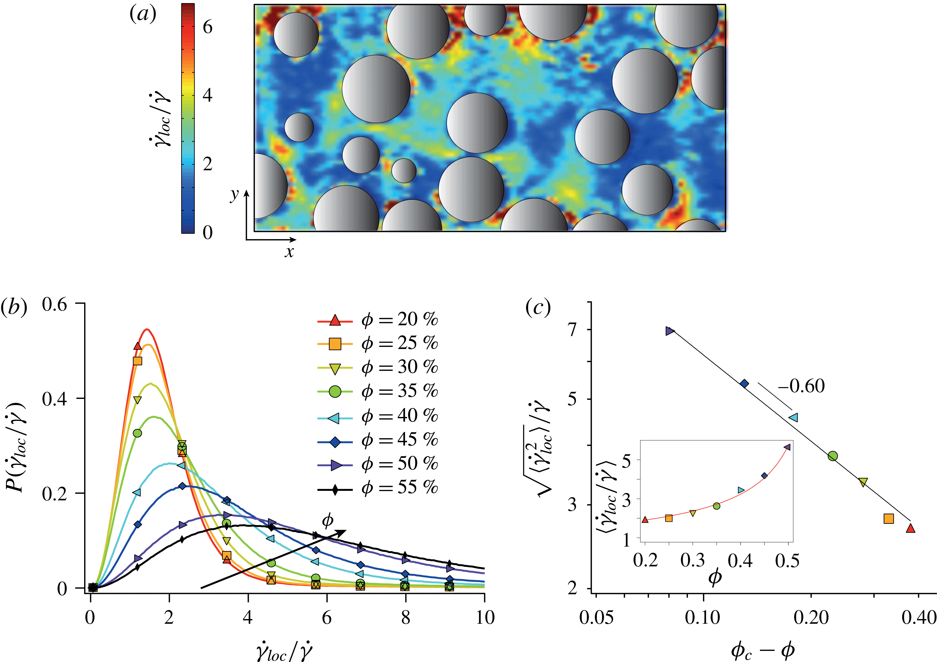
(a) Typical local shear rate map for a suspension with volume fraction
 $\unicode[STIX]{x1D719}=35\,\%$
. (b) Experimental distributions of normalized local shear rate
 $P(\dot{\unicode[STIX]{x1D6FE}}_{loc}/\dot{\unicode[STIX]{x1D6FE}})$
for different volume fractions (the solid line is not a fit but the experimental data, sparse markers are used for sake of clarity). (c)
 $\sqrt{\langle \dot{\unicode[STIX]{x1D6FE}}_{loc}^{2}\rangle }/\dot{\unicode[STIX]{x1D6FE}}$
versus
 $\unicode[STIX]{x1D719}_{c}-\unicode[STIX]{x1D719}$
. The best fit
 $\sqrt{\langle \dot{\unicode[STIX]{x1D6FE}}_{loc}^{2}\rangle }/\dot{\unicode[STIX]{x1D6FE}}\sim (\unicode[STIX]{x1D719}_{c}-\unicode[STIX]{x1D719})^{-\unicode[STIX]{x1D6FD}}$
, with
 $\unicode[STIX]{x1D719}_{c}=0.58$
, yields
 $\unicode[STIX]{x1D6FD}=0.601$
(see text). Inset: mean normalized local shear rate
 $\langle \dot{\unicode[STIX]{x1D6FE}}_{loc}/\dot{\unicode[STIX]{x1D6FE}}\rangle$
versus
 $\unicode[STIX]{x1D719}$
. The line is the best fit by
 $A/(\unicode[STIX]{x1D719}_{c}-\unicode[STIX]{x1D719})^{\unicode[STIX]{x1D6FF}}$
.

5.1.1 Local shear rate
We measure the local shear rate from the experimental 2D velocity fields. To this end, we define the local shear rate by the norm of the symmetric part of the strain tensor:
 $$\begin{eqnarray}\dot{\unicode[STIX]{x1D6FE}}_{loc}=\sqrt{2\left(\frac{\unicode[STIX]{x2202}u}{\unicode[STIX]{x2202}x}\right)^{2}+2\left(\frac{\unicode[STIX]{x2202}v}{\unicode[STIX]{x2202}y}\right)^{2}+\left(\frac{\unicode[STIX]{x2202}u}{\unicode[STIX]{x2202}y}+\frac{\unicode[STIX]{x2202}v}{\unicode[STIX]{x2202}x}\right)^{2}},\end{eqnarray}$$
where
 $\{u,v\}$
are the
 $\{x,y\}$
components of the velocity field. This definition disregards the rotation part of the strain tensor. For a simple shear, one has
 $\dot{\unicode[STIX]{x1D6FE}}_{loc}=\text{const.}=\dot{\unicode[STIX]{x1D6FE}}$
. Figure 10(a) shows a typical local shear rate map, obtained in a suspension with volume fraction
 $\unicode[STIX]{x1D719}=35\,\%$
. The colour scale represents the amplitude of
 $\dot{\unicode[STIX]{x1D6FE}}_{loc}$
normalized by the applied macroscopic shear rate
 $\dot{\unicode[STIX]{x1D6FE}}$
, that is to say the amplification of the shear due to the presence of particles. The local shear rate is highly non-uniform and its value can greatly exceed the macroscopic shear rate. Interestingly, large local shear rates occur preferentially in the vicinity of the particles; however, there is no apparent correlation between large local shear rates and small inter-particle distances.
More quantitatively, we report in figure 10(b) the distribution of normalized local shear rates obtained for various volume fractions. Clearly, the local shear rate exceeds most of the time the imposed macroscopic shear rate, sometimes by one order of magnitude, and this trend accentuates with increasing volume fractions. The mean normalized value
 $\langle \dot{\unicode[STIX]{x1D6FE}}_{loc}\rangle /\dot{\unicode[STIX]{x1D6FE}}$
is plotted versus
 $\unicode[STIX]{x1D719}$
in the inset of figure 10(c). It is found to fit well
 $\langle \dot{\unicode[STIX]{x1D6FE}}_{loc}\rangle /\dot{\unicode[STIX]{x1D6FE}}=A/(\unicode[STIX]{x1D719}_{c}-\unicode[STIX]{x1D719})^{\unicode[STIX]{x1D6FF}}$
. Fixing
 $\unicode[STIX]{x1D719}_{c}=0.58$
this yields
 $A\simeq 0.56$
and
 $\unicode[STIX]{x1D6FF}\simeq 0.7$
. Note that the last point, corresponding to
 $\unicode[STIX]{x1D719}=55\,\%$
, was not included in the fitting procedure since we suspect that it is biased by the deflection of the belt mentioned above. Note also that PIV using smaller boxes resulted in very similar local shear rate distributions with less than 6 % difference on the average.
The trends discussed above may also be interpreted in terms of a macroscopic viscosity. In such case, the relevant quantity to investigate is the second moment of the local shear rate distribution
 $\langle \dot{\unicode[STIX]{x1D6FE}}_{loc}^{2}\rangle$
(Chateau, Ovarlez & Trung Reference Chateau, Ovarlez and Trung2008; Lerner, Dring & Wyart Reference Lerner, Dring and Wyart2012; Dagois-Bogy et al.
Reference Dagois-Bohy, Hormozi, Guazzelli and Pouliquen2015). Values of this quantity have recently been obtained by Trulson et al. from numerical simulations of dense frictional suspensions (Trulsson, DeGiuli & Wyart Reference Trulsson, DeGiuli and Wyart2016). They report that
 $\sqrt{\langle \dot{\unicode[STIX]{x1D6FE}}_{loc}^{2}\rangle }/\dot{\unicode[STIX]{x1D6FE}}\sim (J/\unicode[STIX]{x1D707})^{-1/3}$
, where
 $J=\dot{\unicode[STIX]{x1D6FE}}\unicode[STIX]{x1D702}_{f}/P$
is the viscous number, with
 $P$
the confining pressure and
 $\unicode[STIX]{x1D707}$
the suspension macroscopic friction coefficient. Since
 $\unicode[STIX]{x1D702}_{s}/\unicode[STIX]{x1D702}_{f}=\unicode[STIX]{x1D70E}/\dot{\unicode[STIX]{x1D6FE}}\unicode[STIX]{x1D702}_{f}=\unicode[STIX]{x1D707}/J$
, this results in
 $\sqrt{\langle \dot{\unicode[STIX]{x1D6FE}}_{loc}^{2}\rangle }/\dot{\unicode[STIX]{x1D6FE}}\sim (\unicode[STIX]{x1D702}_{s}/\unicode[STIX]{x1D702}_{f})^{1/3}$
. Combining this with
 $\unicode[STIX]{x1D702}_{s}/\unicode[STIX]{x1D702}_{f}\sim (\unicode[STIX]{x1D719}_{c}-\unicode[STIX]{x1D719})^{-2}$
and using
 $\unicode[STIX]{x1D719}_{c}=0.58$
(Boyer, Guazzelli & Pouliquen Reference Boyer, Guazzelli and Pouliquen2011) leads to
 $\sqrt{\langle \dot{\unicode[STIX]{x1D6FE}}_{loc}^{2}\rangle }/\dot{\unicode[STIX]{x1D6FE}}\sim (\unicode[STIX]{x1D719}_{c}-\unicode[STIX]{x1D719})^{-2/3}$
, which is in fairly good agreement with the measured scaling, as figure 10(c) shows.
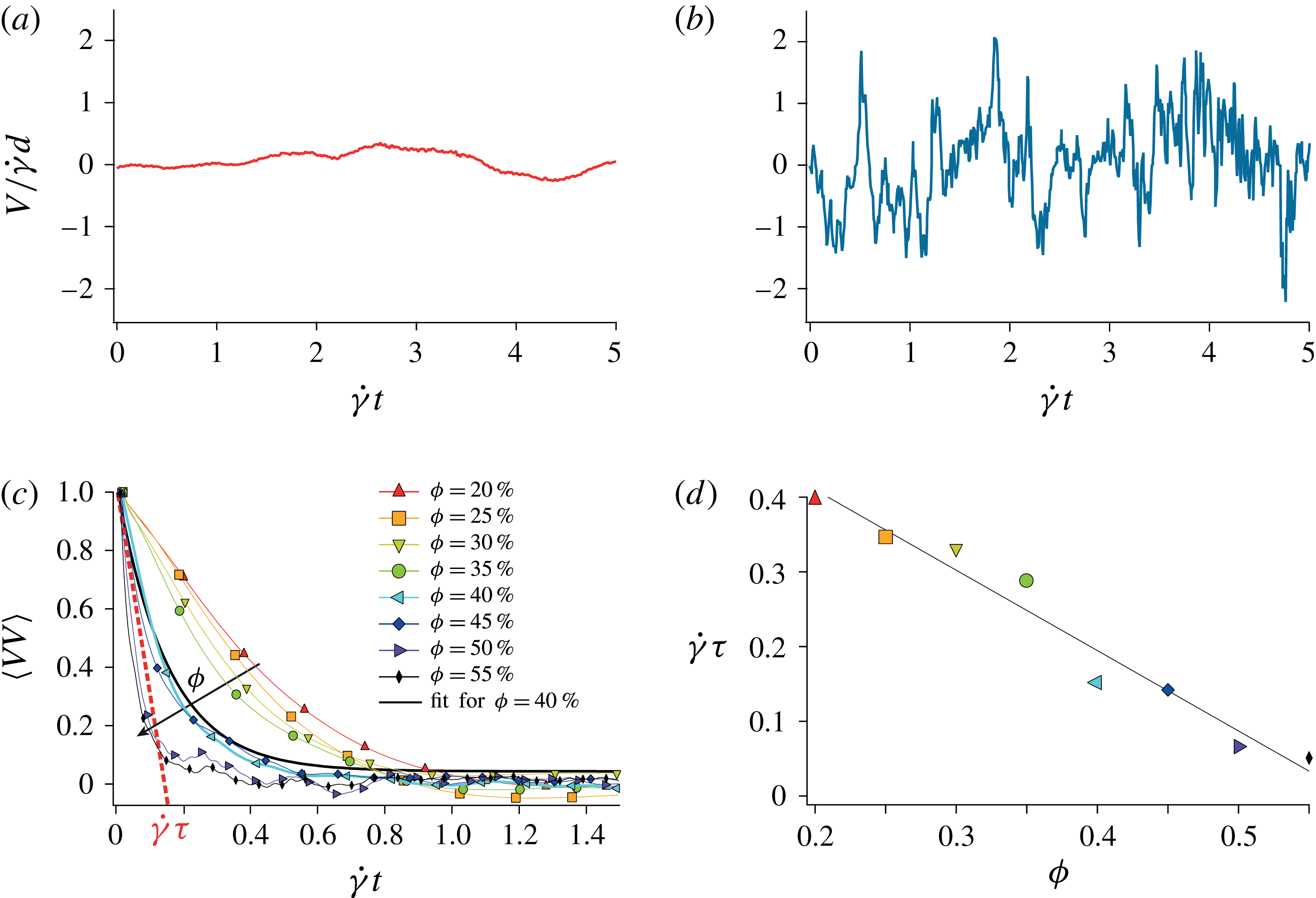
(a,b) Lagrangian velocity transverse to the flow of a tracer passively advected by the suspending liquid
 $V$
, as a function of the strain
 $\dot{\unicode[STIX]{x1D6FE}}t$
. (a)
 $\unicode[STIX]{x1D719}=20\,\%$
and (b)
 $\unicode[STIX]{x1D719}=50\,\%$
. (c) Average Lagrangian velocity auto-correlation function
 $\langle VV\rangle$
obtained for different volume fractions versus strain. The velocity auto-correlation functions fit well
 $\text{e}^{-\dot{\unicode[STIX]{x1D6FE}}t/\dot{\unicode[STIX]{x1D6FE}}\unicode[STIX]{x1D70F}}$
, where
 $\unicode[STIX]{x1D70F}$
denotes the correlation time. (d) Correlation strain
 $\dot{\unicode[STIX]{x1D6FE}}\unicode[STIX]{x1D70F}$
versus
 $\unicode[STIX]{x1D719}$
and corresponding linear fit
 $\dot{\unicode[STIX]{x1D6FE}}\unicode[STIX]{x1D70F}=0.62-1.08\,\unicode[STIX]{x1D719}$
.

5.1.2 Lagrangian correlation time
The second important quantity of the suspending liquid flow is the persistence time of the velocity fluctuations induced by the particles. Figures 11(a) and 11(b) show the transverse Lagrangian velocity
 $V$
(perpendicular to the flow) of a passive tracer advected by the fluid at a low and a large volume fraction, respectively. Consistently with the magnitude of the local shear, more concentrated particulate suspensions develop velocity fluctuations with larger amplitudes. However these fluctuations are found to persist on a much shorter time as
 $\unicode[STIX]{x1D719}$
increases. The duration
 $t_{c}$
for which a segment is coherently stretched by the flow is directly prescribed by this persistence time, which we define from the Lagrangian velocity auto-correlation functions. As shown in figure 11(c), these functions decorrelate exponentially with strain. In the range of volume fraction investigated, the dimensionless correlation time
 $\dot{\unicode[STIX]{x1D6FE}}\unicode[STIX]{x1D70F}$
, inferred from this exponential decay, decreases linearly with
 $\unicode[STIX]{x1D719}$
as
 $$\begin{eqnarray}\dot{\unicode[STIX]{x1D6FE}}\unicode[STIX]{x1D70F}\simeq 0.62-1.08\,\unicode[STIX]{x1D719}\end{eqnarray}$$
(see figure 11
d). We expect
 $t_{c}$
to be of the order of
 $\unicode[STIX]{x1D70F}$
, and thus write
 $$\begin{eqnarray}t_{c}=\unicode[STIX]{x1D6FC}\unicode[STIX]{x1D70F},\end{eqnarray}$$
with
 $\unicode[STIX]{x1D6FC}$
an order one constant. Note that, as shown in figure 7, this persistence time (
 ${\lesssim}\dot{\unicode[STIX]{x1D6FE}}^{-1}$
) is much shorter than the observation period (
 ${\gtrsim}10\dot{\unicode[STIX]{x1D6FE}}^{-1}$
).
5.1.3 Multiplicative stretching process
With information about the local shear rates and their persistence time at hand, we now explain the elongations of fluid material lines as a sequence of uncorrelated cycles of stretching. During the first cycle of duration
 $t_{c}$
, a given segment of a material line is elongated by the local shear rate
 $\dot{\unicode[STIX]{x1D6FE}}_{loc,1}$
resulting in a stretching
 $$\begin{eqnarray}\unicode[STIX]{x0394}\unicode[STIX]{x1D70C}_{1}=\sqrt{1+(\dot{\unicode[STIX]{x1D6FE}}_{loc,1}t_{c})^{2}/2},\end{eqnarray}$$
where
 $\dot{\unicode[STIX]{x1D6FE}}_{loc,1}$
is a local shear rate whose probability is prescribed by the distribution
 $P(\dot{\unicode[STIX]{x1D6FE}}_{loc}/\dot{\unicode[STIX]{x1D6FE}})$
, cf. figure 10(b). After the duration
 $t_{c}$
, the local velocity field decorrelates and the local shear rate map is entirely redistributed. The segment then experiences a new local shear rate
 $\dot{\unicode[STIX]{x1D6FE}}_{loc,2}$
, which at
 $t=2t_{c}$
yields
 $\unicode[STIX]{x1D70C}=\unicode[STIX]{x0394}\unicode[STIX]{x1D70C}_{1}\sqrt{1+(\dot{\unicode[STIX]{x1D6FE}}_{loc,2}t_{c})^{2}/2}$
, and so on. The total elongation at time
 $t$
, after
 $N=t/t_{c}$
cycles, is the product of all the elementary elongations occurring at each cycle
 $\unicode[STIX]{x1D70C}(t)=\prod _{i=1}^{N=t/t_{c}}\!\unicode[STIX]{x0394}\unicode[STIX]{x1D70C}_{i}$
. The logarithm of this expression can be written as a sum
 $$\begin{eqnarray}\ln \unicode[STIX]{x1D70C}\equiv \mathop{\sum }_{i=1}^{t/t_{c}}\ln \unicode[STIX]{x0394}\unicode[STIX]{x1D70C}_{i}=\frac{1}{2}\mathop{\sum }_{i=1}^{t/t_{c}}\ln [1+(\dot{\unicode[STIX]{x1D6FE}}_{loc,i}t_{c})^{2}/2].\end{eqnarray}$$
Since the elementary stretchings are independent, the distribution of
 $\ln \unicode[STIX]{x1D70C}$
is expected, by virtue of the central limit theorem, to be normal. This multiplicative stretching model thus predicts
 $\unicode[STIX]{x1D70C}$
to converge, after a few
 $t/t_{c}$
cycles, to a log-normal distribution. This prediction is in agreement with the experimental results shown in figure 7(b). The distribution of
 $\ln \unicode[STIX]{x1D70C}$
, i.e. the normal distribution, is written as
 $$\begin{eqnarray}P(x=\ln \unicode[STIX]{x1D70C})=\frac{1}{\sqrt{2\unicode[STIX]{x03C0}}\unicode[STIX]{x1D70E}}\,\text{e}^{-(x-\unicode[STIX]{x1D707})^{2}/2\unicode[STIX]{x1D70E}^{2}},\end{eqnarray}$$
with a non-zero mean
 $$\begin{eqnarray}\unicode[STIX]{x1D707}\equiv \langle \ln \unicode[STIX]{x1D70C}\rangle =\frac{\langle \ln \unicode[STIX]{x0394}\unicode[STIX]{x1D70C}\rangle }{\dot{\unicode[STIX]{x1D6FE}}t_{c}}\,\dot{\unicode[STIX]{x1D6FE}}t,\end{eqnarray}$$
and variance
 $$\begin{eqnarray}\unicode[STIX]{x1D70E}^{2}\equiv \langle \ln ^{2}\unicode[STIX]{x1D70C}\rangle -\unicode[STIX]{x1D707}^{2}=\frac{\langle \ln ^{2}\unicode[STIX]{x0394}\unicode[STIX]{x1D70C}\rangle -\langle \ln \unicode[STIX]{x0394}\unicode[STIX]{x1D70C}\rangle ^{2}}{\dot{\unicode[STIX]{x1D6FE}}t_{c}}\,\dot{\unicode[STIX]{x1D6FE}}t.\end{eqnarray}$$
Both the mean and the variance of the distribution of
 $\ln \unicode[STIX]{x1D70C}$
increase linearly with time. They also vary with the particulate volume fraction due to the
 $\unicode[STIX]{x1D719}$
-dependence of
 $\dot{\unicode[STIX]{x1D6FE}}_{loc}$
and
 $t_{c}$
. This variation with
 $\unicode[STIX]{x1D719}$
is better appreciated by recasting equations (5.8) and (5.9) into
 $$\begin{eqnarray}\displaystyle & \displaystyle \unicode[STIX]{x1D707}=f(\unicode[STIX]{x1D719})\,\dot{\unicode[STIX]{x1D6FE}}t, & \displaystyle\end{eqnarray}$$
 $$\begin{eqnarray}\displaystyle & \displaystyle \unicode[STIX]{x1D70E}^{2}=g(\unicode[STIX]{x1D719})\,\dot{\unicode[STIX]{x1D6FE}}t, & \displaystyle\end{eqnarray}$$
with
 $f(\unicode[STIX]{x1D719})\equiv \langle \ln \unicode[STIX]{x0394}\unicode[STIX]{x1D70C}\rangle /\dot{\unicode[STIX]{x1D6FE}}t_{c}$
and
 $g(\unicode[STIX]{x1D719})\equiv (\langle \ln ^{2}\unicode[STIX]{x0394}\unicode[STIX]{x1D70C}\rangle -\langle \ln \unicode[STIX]{x0394}\unicode[STIX]{x1D70C}\rangle ^{2})/\dot{\unicode[STIX]{x1D6FE}}t_{c}$
depending only on
 $\unicode[STIX]{x1D719}$
. Note that
 $f(\unicode[STIX]{x1D719})$
and
 $g(\unicode[STIX]{x1D719})$
are crucial quantities. Since the time dependency is known, they contain all the information about the asymptotics of the stretching laws in suspensions.
The multiplicative stretching model not only explains the origin of the log-normal distributions of elongations measured experimentally, but also the exponential increase of the mean elongation
 $\unicode[STIX]{x1D70C}$
and variance
 $\unicode[STIX]{x1D70E}_{\unicode[STIX]{x1D70C}}^{2}$
shown in figure 7. Indeed, the mean and variance of the (log-normal) distribution of
 $\unicode[STIX]{x1D70C}$
can be deduced from the mean and the variance of the (normal) distribution of
 $\ln \unicode[STIX]{x1D70C}$
following
 $$\begin{eqnarray}\langle \unicode[STIX]{x1D70C}\rangle =\text{e}^{(f+g/2)\dot{\unicode[STIX]{x1D6FE}}t},\end{eqnarray}$$
and
 $$\begin{eqnarray}\unicode[STIX]{x1D70E}_{\unicode[STIX]{x1D70C}}^{2}=(\text{e}^{g\dot{\unicode[STIX]{x1D6FE}}t}-1)\text{e}^{(2f+g)\dot{\unicode[STIX]{x1D6FE}}t}\simeq \text{e}^{2(f+g)\dot{\unicode[STIX]{x1D6FE}}t},\end{eqnarray}$$
the last simplification in
 $\unicode[STIX]{x1D70E}_{\unicode[STIX]{x1D70C}}^{2}$
becoming true after a few
 $t_{c}$
.
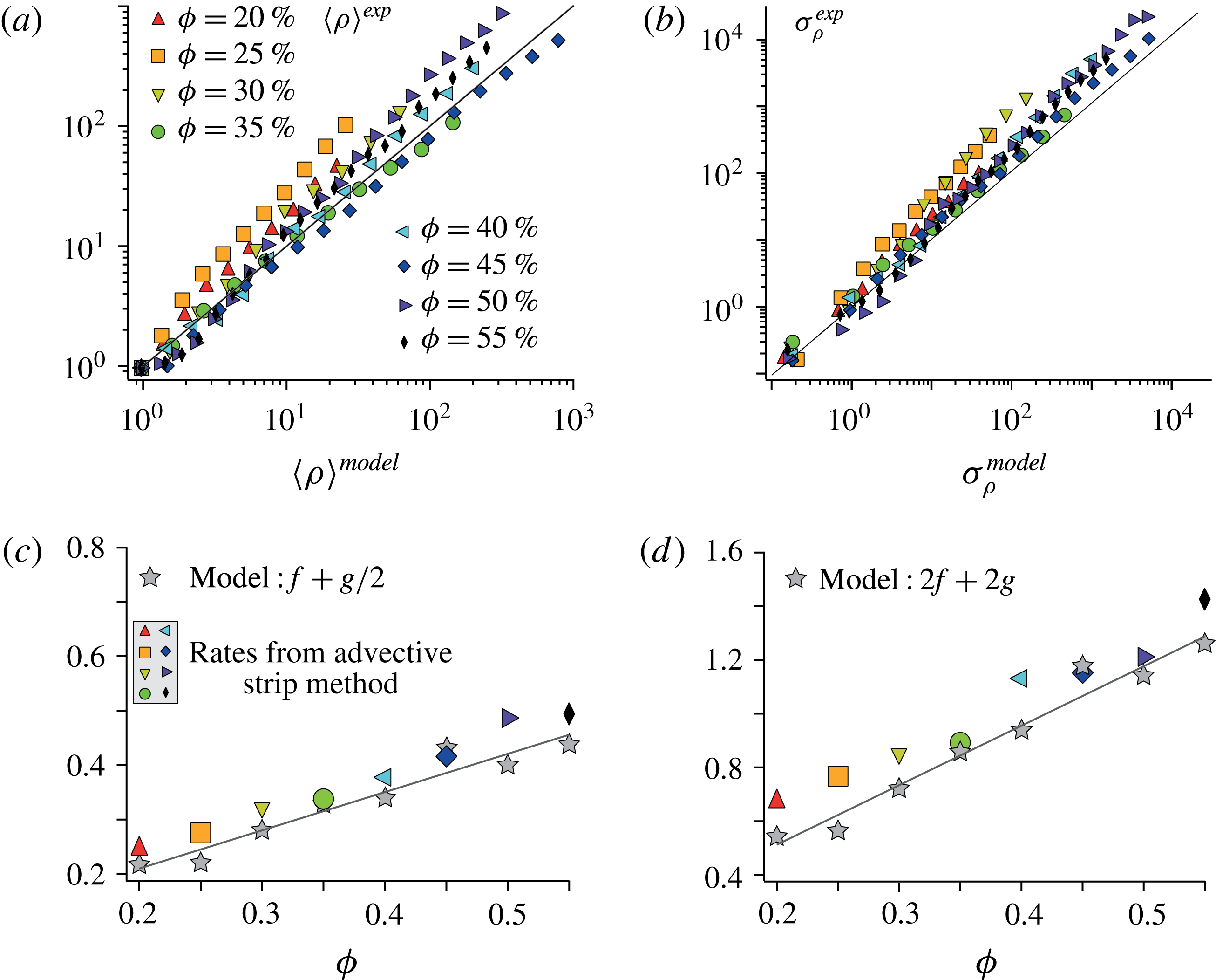
Comparison between the experimental stretching (extracted from figure 8) and the multiplicative stretching model. (a,b) Mean elongation
 $\langle \unicode[STIX]{x1D70C}\rangle$
and standard deviation
 $\unicode[STIX]{x1D70E}_{\unicode[STIX]{x1D70C}}$
. The values from the advective strip method are plotted versus those predicted by the multiplicative stretching model. (c) Comparison between the exponential rates of the mean elongation
 $\unicode[STIX]{x1D705}_{\unicode[STIX]{x1D70C}}$
obtained from the advective strip method (see figure 8
a) and the model prediction
 $f+g/2$
(5.12). (d) Comparison between the exponential rates of the variance of the elongation
 $2\unicode[STIX]{x1D705}_{\unicode[STIX]{x1D70E}_{\unicode[STIX]{x1D70C}}}$
(see figure 8
b) and the model prediction
 $2(f+g)$
(5.13).

Furthermore, the particulate volume fraction dependence of
 $f(\unicode[STIX]{x1D719})$
and
 $g(\unicode[STIX]{x1D719})$
can be computed from the persistence time
 $t_{c}$
and the distribution of local shear rates, using (5.10) and (5.11) together with (5.8) and (5.9). In the experimental range
 $20\,\%<\unicode[STIX]{x1D719}<55\,\%$
, this yields
 $$\begin{eqnarray}f(\unicode[STIX]{x1D719})\simeq 0.104+0.298\,\unicode[STIX]{x1D719},\end{eqnarray}$$
and
 $$\begin{eqnarray}g(\unicode[STIX]{x1D719})\simeq -0.069+0.810\,\unicode[STIX]{x1D719},\end{eqnarray}$$
with the structure constant
 $\unicode[STIX]{x1D6FC}$
, set once and for all
 $\unicode[STIX]{x1D719}$
, to 0.3 for computing
 $\unicode[STIX]{x1D707}$
, and to 3.9 for computing
 $\unicode[STIX]{x1D70E}^{2}$
. These rates
 $f$
and
 $g$
both increase with
 $\unicode[STIX]{x1D719}$
, in agreement with the experimental trends. Note that this dependence on the volume fraction is non-trivial, since
 $f$
and
 $g$
result from the product of
 $\dot{\unicode[STIX]{x1D6FE}}_{loc}$
and
 $t_{c}$
, which have opposite trends with
 $\unicode[STIX]{x1D719}$
: the former increases whereas the latter decreases with increasing
 $\unicode[STIX]{x1D719}$
.
The predictions of the multiplicative stretching model are compared to the experimental stretching laws obtained by the Diffusive Strip Method in figure 12. The agreement is good for all volume fractions and all strains, which suggests that the multiplicative stretching model presented above captures the relevant mechanisms at the origin of the stretching laws.
5.2 Comments on the stretching process
Stretching of material elements in nature, may they be passive like in the present case, or with internal restoration forces like polymers (Shaqfeh & Koch Reference Shaqfeh and Koch1992; Afonso & Vincenzi Reference Afonso and Vincenzi2005), may have different origins. The stochastic models to describe them usually present a net drift, and a random noise terms. The relative amplitudes of these two contributions are in our analysis given by
 $f(\unicode[STIX]{x1D719})$
and
 $g(\unicode[STIX]{x1D719})$
, respectively (see (5.10) and (5.11)). The first term sets the growth of
 $\langle \ln \unicode[STIX]{x1D70C}\rangle$
, while the second sets that of
 $\langle \ln ^{2}\!\unicode[STIX]{x1D70C}\rangle -\langle \ln \unicode[STIX]{x1D70C}\rangle ^{2}$
. At a microscopic level, the growth of a given material line depends on its orientation with that of the local velocity gradient. The line length
 $l(t)$
may increase or decrease depending on whether it is aligned with a diverging or compressive region of the flow. For instance, in a flow corresponding to the pure Brownian motion limit (Cocke Reference Cocke1971), for which
 $\dot{\unicode[STIX]{x1D70C}}/\unicode[STIX]{x1D70C}=B(t)$
with
 $B(t)$
a zero-mean, delta-correlated noise, i.e.
 $\langle B(t)\rangle =0$
and
 $\langle B(t^{\prime })B(t^{\prime \prime })\rangle =(1/\unicode[STIX]{x1D70F}_{0})\unicode[STIX]{x1D6FF}(t^{\prime }-t^{\prime \prime })$
, these two contributions are balanced and the net line growth
 $\text{d}\ln \unicode[STIX]{x1D70C}(t)/\text{d}t=\dot{l(t)}/l(t)$
is, on averaging over all directions, identically zero. In that case, representative of
 $t_{c}\rightarrow 0$
, the material lines only grow through the contribution of the fluctuations of
 $B(t)$
, which results in
 $\text{d}\langle \ln \unicode[STIX]{x1D70C}\rangle /\text{d}t=0$
, and
 $\langle (\ln \unicode[STIX]{x1D70C})^{2}\rangle \sim 2t/\unicode[STIX]{x1D70F}_{0}$
: the logarithm of the elongation diffuses.
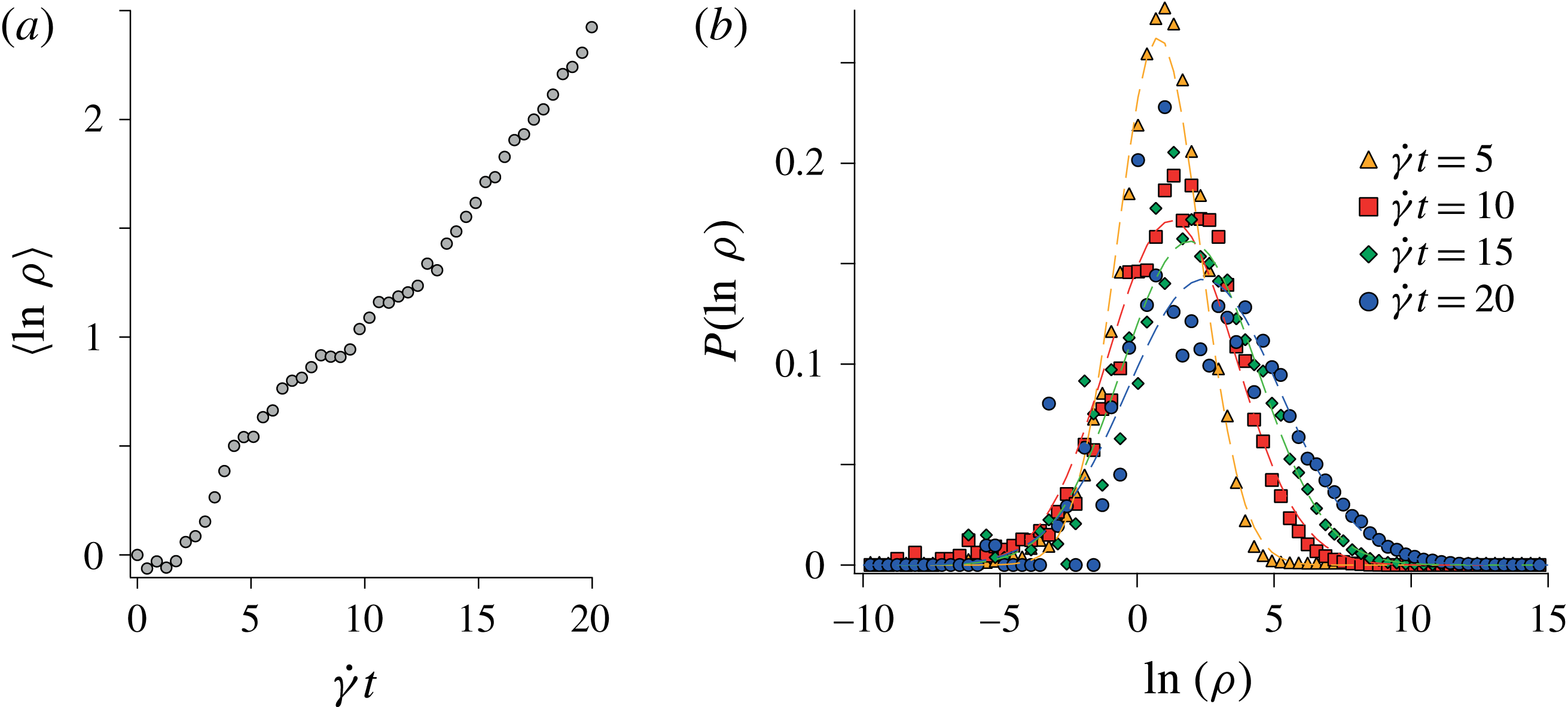
(a) Mean logarithm of the material line elongations,
 $\langle \ln \unicode[STIX]{x1D70C}\rangle$
versus
 $\dot{\unicode[STIX]{x1D6FE}}t$
for a suspension of volume fraction
 $\unicode[STIX]{x1D719}=35\,\%$
. (b) PDF of the logarithm of the material line elongations
 $P(\ln \unicode[STIX]{x1D70C})$
at successive times.

In particulate suspensions, the situation is different since if the direction of the stretch indeed changes at random, it has a finite persistence time. In such case, it has been shown that material lines tend to preferentially align in the direction of elongations (see Cocke (Reference Cocke1969), Orszag (Reference Orszag1970), Girimaji & Pope (Reference Girimaji and Pope1990), Duplat & Villermaux (Reference Duplat and Villermaux2000) and also (5.5)). Thus, over an observation period larger than the (non-zero) correlation time
 $t_{c}$
, we expect
 $$\begin{eqnarray}\frac{\text{d}}{\text{d}t}\langle \ln \unicode[STIX]{x1D70C}\rangle >0.\end{eqnarray}$$
This agrees with our measurements shown in figure 13(a): the finite persistence time of the stretching field results in a positive drift term:
 $f(\unicode[STIX]{x1D719})>0$
. Although some material lines are subject to compression (see the negative values on the distribution of
 $\ln \unicode[STIX]{x1D70C}$
in figure 13
b), on average, the logarithm of the elongations
 $\langle \ln \unicode[STIX]{x1D70C}\rangle$
increases with time. Material lines in particulate suspensions thus grow from the contribution of both a drift and a noise. The stretching process thus corresponds to a noisy multiplicative sequence of correlated motions, like the random Sine Flow (Meunier & Villermaux Reference Meunier and Villermaux2010), or porous media flows (Le Borgne et al.
Reference Le Borgne, Dentz and Villermaux2015). Porous media and sheared particulate suspensions have similar exponential stretching laws. This is true in 3D systems, as in both cases the fluid trajectories are chaotic. Note, however, that for 2D systems the implications of steadiness change the picture qualitatively. In a 2D porous media, the flow is steady and there are only two degrees of freedom : the flow is thus not chaotic. The elongation of material lines in 2D synthetic porous media have been shown to grow algebraically rather than exponentially (Le Borgne et al.
Reference Le Borgne, Dentz and Villermaux2015). Conversely, in 2D sheared suspensions, the time dependence of the flow allows the system to be chaotic (Metzger et al.
Reference Metzger, Pham and Butler2013). One therefore expect to observe exponential stretching laws in sheared particulate suspensions also in purely 2D configurations.
5.3 Further remarks
We would like to point out certain limitations of the present study. First, the present findings and their analysis are restricted to the particulate volume fraction
 $20\,\%\leqslant \unicode[STIX]{x1D719}\leqslant 55\,\%$
, for which material lines in the suspending liquid stretch exponentially with strain. This is not necessarily the case outside this range. In particular, as
 $\unicode[STIX]{x1D719}\rightarrow 0$
, this exponential trend must cross over to linear since the elongation of material lines in a simple shear is linear with strain. However, we anticipate that the exponential trend could hold down to fairly low volume fractions, but only emerge after increasingly large strains, since the velocity correlation time in the dilute limit should follow
 $\unicode[STIX]{x1D70F}\sim (\dot{\unicode[STIX]{x1D6FE}}\unicode[STIX]{x1D719})^{-1}$
and diverge at low
 $\unicode[STIX]{x1D719}$
. Further investigations are needed to characterize this dilute regime (
 $\unicode[STIX]{x1D719}<20\,\%$
).
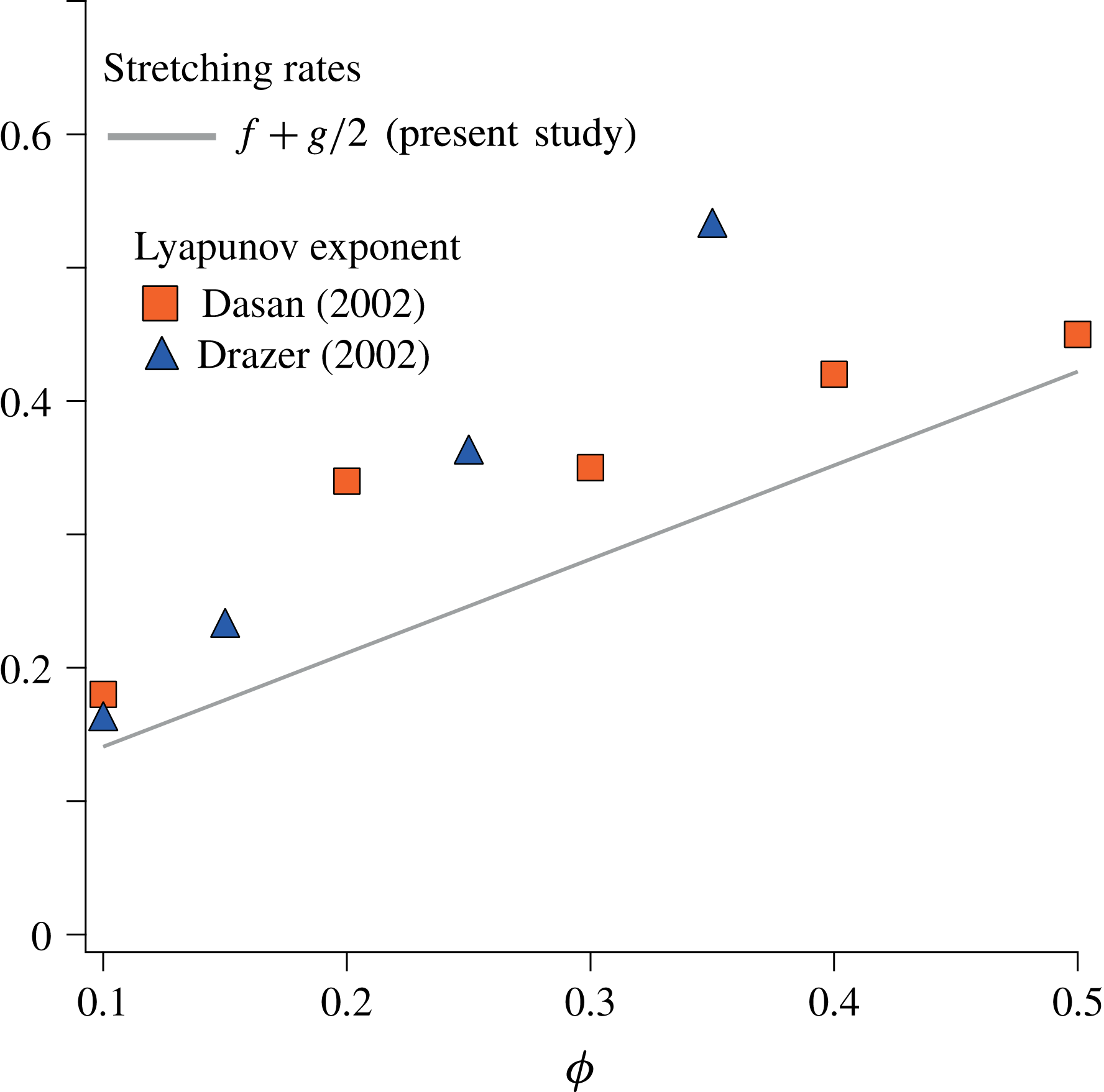
Comparison between the stretching rates obtained in the present study and the largest Lyapunov exponent obtained from 3D Stokesian dynamics simulations (Dasan et al. Reference Dasan, Ramamohan, Singh and Nott2002; Drazer et al. Reference Drazer, Koplik, Khusid and Acrivos2002).

Second, the PIV measurements performed here are two-dimensional and provide the fluid velocity projected in the (
 $xy$
) plane only. They therefore neglect part of the stretching of the material lines, namely that involving deformations in the vorticity direction (
 $z$
). However, we believe that they resolve the stretching mechanism and most of its magnitude for the following reasons. (i) These measurements resolve the fluid displacements in the gradient direction (
 $y$
), which is the only direction for which displacements couple with the main shear flow to produce enhanced stretching. The fluctuations in the vorticity direction are thus expected to produce less stretching than those occurring in the gradient direction. (ii) Particles in a shear flow rotate mainly about the vorticity axis, thereby inducing fluid disturbances mostly in the velocity-gradient plane, which we consider. Here again, the effects of the velocity disturbances induced by the particle rotation should be smaller in the vorticity direction than those occurring in the velocity-gradient plane. (iii) More quantitatively, the stretching rates
 $f+g/2$
predicted by the present model based on 2D data are in good agreement with the largest Lyapunov exponents obtained from 3D Stokesian simulations, see figure 14. From the above considerations, it is likely that the mechanisms at the origin of the scalar dispersion, stretching and subsequent mixing are well characterized by the present measurements, even though those are limited to the information contained in the
 $xy$
plane.
Third, as already mentioned in § 3, the stretching of material lines is exponential at every scale, but the stretching of a material blob with thickness
 $s_{0}$
is expected to follow that of material lines only if its thickness is smaller than the correlation scale of the fluid motion, which is of order
 $d$
(in the other case, the blob is first essentially stretched by the macroscopic shear
 $\dot{\unicode[STIX]{x1D6FE}}$
until
 $s\leqslant d$
). In the following, we will therefore only consider the relevant case
 $s_{0}\leqslant d$
.
The latter considerations have important consequences on the estimation of the blob thickness
 $s$
, hence on the mixing time that we will address in the next section. For an arbitrary elongation
 $w/w_{0}$
in the vorticity direction (
 $z$
), mass conservation gives
 $s_{0}l_{0}w_{0}=s(t)l(t)w(t)$
. However, in light of the above discussion, the flow is assumed to be two-dimensional with
 $w/w_{0}\ll l/l_{0}$
. Mass conservation thus results in
 $$\begin{eqnarray}s_{0}l_{0}=s(t)l(t).\end{eqnarray}$$
Using direct image analysis, we have checked that this is experimentally verified. A blob with initial surface
 $s_{0}l_{0}$
being converted into a strip with length
 $l(t)$
and thickness
 $s(t)$
indeed obeys, before it starts mixing, equation (5.17), suggesting that the flow is indeed area preserving.
6 Implications for mixing
In such area-preserving flow, the thickness
 $s(t)$
of a distorted blob decreases in inverse proportion of its length
 $l(t)$
according to (5.17). As recalled in the introduction, the mixing time for a given blob portion of thickness
 $s$
is reached when its compression rate
 $-{\dot{s}}/s$
is balanced by its rate of diffusive broadening
 $D/s^{2}$
. At that time, called the mixing time, the scalar concentration carried by that portion of the blob starts to significantly decay i.e., mix. Since in particulate suspensions
 $\unicode[STIX]{x1D70C}=l(t)/l_{0}=\text{e}^{\unicode[STIX]{x1D705}\dot{\unicode[STIX]{x1D6FE}}t}$
, the mixing time is written as
 $t_{mix}\simeq \dot{\unicode[STIX]{x1D6FE}}^{-1}\ln (\unicode[STIX]{x1D705}Pe)/(2\unicode[STIX]{x1D705})$
.
We also found that the logarithm of the elongations of an ensemble of such material lines is normally distributed, with a mean and a variance growing linearly with time following
 $\unicode[STIX]{x1D707}=\langle \ln \unicode[STIX]{x1D70C}\rangle =f(\unicode[STIX]{x1D719})\dot{\unicode[STIX]{x1D6FE}}t$
and
 $\unicode[STIX]{x1D70E}^{2}=g(\unicode[STIX]{x1D719})\dot{\unicode[STIX]{x1D6FE}}t$
(see (5.10) and (5.11), respectively). These results are illustrated in figure 15(a). Since, similarly to the logarithm of the elongations, the stretching rates,
 $\unicode[STIX]{x1D705}\dot{\unicode[STIX]{x1D6FE}}=\ln \unicode[STIX]{x1D70C}/t$
are normally distributed, the median mixing time, obtained for the mean stretching rate, i.e. for
 $\langle \unicode[STIX]{x1D705}\dot{\unicode[STIX]{x1D6FE}}\rangle =\langle \ln \unicode[STIX]{x1D70C}\rangle /t=\unicode[STIX]{x1D707}/t=f(\unicode[STIX]{x1D719})\dot{\unicode[STIX]{x1D6FE}}$
, is
 $$\begin{eqnarray}t_{mix}^{med}\approx \frac{1}{2f(\unicode[STIX]{x1D719})\dot{\unicode[STIX]{x1D6FE}}}\ln (f(\unicode[STIX]{x1D719})Pe).\end{eqnarray}$$
Considering a blob distorted in such a way that it samples all the possible elongations in the global statistics, the above estimate provides the time at which half of the blob has reached its mixing time. The logarithmic dependence of the mixing time on the Péclet number is different from that obtained in a simple shear flow (without particles) for which
 $\unicode[STIX]{x1D70C}\simeq \dot{\unicode[STIX]{x1D6FE}}t$
yields
 $t_{mix}\simeq \dot{\unicode[STIX]{x1D6FE}}^{-1}Pe^{1/3}$
. Introducing particles in a viscous fluid therefore becomes more and more efficient at reducing the mixing time as the Péclet number increases. In the present study, the Péclet number is
 $Pe\sim 10^{6}$
. The median mixing time for
 $\unicode[STIX]{x1D719}=35\,\%$
is thus
 $t_{mix}^{med}\simeq 30/\dot{\unicode[STIX]{x1D6FE}}$
, which has to be compared with
 $t_{mix}\simeq 100/\dot{\unicode[STIX]{x1D6FE}}$
in a pure shear flow. Note that varying the volume fraction from 20 % to 55 % increases
 $f(\unicode[STIX]{x1D719})$
only by a typical factor of 2, which decreases the median mixing time by approximately the same moderate factor.
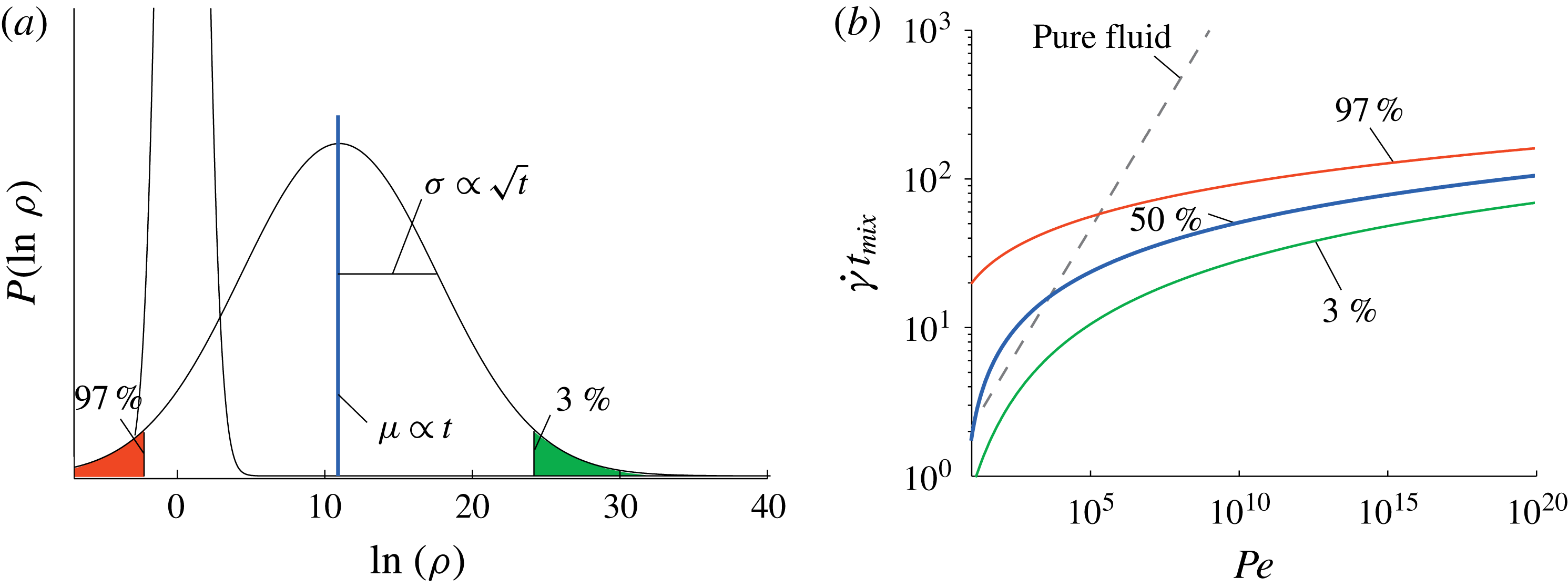
(a) Evolution of the distribution
 $P(\ln \unicode[STIX]{x1D70C})$
of the logarithm of the material line elongations in a particulate suspension. The mean of the distribution
 $\unicode[STIX]{x1D707}\sim t$
and its standard deviation
 $\unicode[STIX]{x1D70E}\sim \sqrt{t}$
. (b) Dimensionless mixing times
 $\dot{\unicode[STIX]{x1D6FE}}t_{mix}$
in a suspension (
 $\unicode[STIX]{x1D719}=35\,\%$
) as a function of
 $Pe$
. The median (blue line), the most stretched
 $t_{mix}^{3\,\%}$
(green line), and the less stretched
 $t_{mix}^{97\,\%}$
(red line) dimensionless mixing times can be compared to the dimensionless mixing time
 ${\sim}Pe^{1/3}$
expected in a pure fluid (dashed line).

In practical situations, mixing half of the scalar may not be the relevant question, precisely because, in particulate suspensions, elongations are, as seen in figure 5, broadly distributed. So are mixing times. To address this point, we estimate, for the same conditions as previously, the mixing times for the portions of the blob that undergo the largest and the lowest stretching rates respectively, i.e. the mixing times corresponding to both tails of the distribution (highlighted in figure 15
a). The 3 % most strongly stretched portions of the blob are bounded by
 $\ln \unicode[STIX]{x1D70C}=\unicode[STIX]{x1D707}+2\unicode[STIX]{x1D70E}$
. The expression
 $-{\dot{s}}/s=D/s^{2}$
results in
 $2f(\unicode[STIX]{x1D719})\dot{\unicode[STIX]{x1D6FE}}t+4\sqrt{g(\unicode[STIX]{x1D719})\dot{\unicode[STIX]{x1D6FE}}t}=\ln [(f(\unicode[STIX]{x1D719})+\sqrt{g(\unicode[STIX]{x1D719})/\dot{\unicode[STIX]{x1D6FE}}t})Pe]$
, which yields the mean field mixing time
 $t_{mix}^{3\,\%}\simeq 14/\dot{\unicode[STIX]{x1D6FE}}$
. On the other end of the distribution, the less stretched portions of the blob, bounded by
 $\ln \unicode[STIX]{x1D70C}=\unicode[STIX]{x1D707}-2\unicode[STIX]{x1D70E}$
, reach their mixing time at
 $t_{mix}^{97\,\%}\simeq 64/\dot{\unicode[STIX]{x1D6FE}}$
, later than if it were sheared in a pure fluid. In figure 15(b), the median (blue line), the most stretched
 $t_{mix}^{3\,\%}$
(green line), and the less stretched
 $t_{mix}^{97\,\%}$
(red line) dimensionless mixing times are plotted as a function of the Péclet number. This shows that if the concern is to mix essentially all the scalar, large Péclet numbers (
 $\gg 10^{5}$
) are required before mixing in a suspension becomes more efficient than in a pure fluid. Persistent poorly stretched regions are deterring. The relative width
 $\unicode[STIX]{x1D70E}/\unicode[STIX]{x1D707}$
of the stretching rate distribution decreases in time like
 $t^{-1/2}$
but this only mildly decreases the spreading of the mixing times as
 $Pe$
increases, since
 $t_{mix}\propto \ln Pe$
. For instance, at
 $Pe=10^{20}$
, the mixing times remain fairly distributed with
 $t_{mix}^{97\,\%}/t_{mix}^{3\,\%}>2$
.
Finally, the results obtained on the stretching laws must be related to the overall dispersion of the blob. In a random flow, line stretching, and dispersion, are two different things: because the extent of the area occupied by the blob grows more slowly than the area where the scalar constitutive of the blob is dispersed, the blob will at some point unavoidably reconnect and merge by overlapping onto itself (Duplat & Villermaux Reference Duplat and Villermaux2008). Let us see how: after the mixing time, a scalar blob with length growing like
 $l(t)=l_{0}\text{e}^{\dot{\unicode[STIX]{x1D6FE}}t}$
has a transverse concentration profile whose width is confined to the Batchelor scale
 $\sqrt{Dt}$
. The area
 ${\mathcal{A}}$
occupied by the scalar is thus
 ${\mathcal{A}}=\sqrt{Dt}\,l_{0}\text{e}^{\dot{\unicode[STIX]{x1D6FE}}t}$
, growing exponentially in time. Now, the spatial support of the blob undergoes a dispersion induced by the particle effective dispersion coefficient
 $D_{eff}\sim \dot{\unicode[STIX]{x1D6FE}}d^{2}$
(Eckstein et al.
Reference Eckstein, Bailey and Shapiro1977). The total area explored by the blob of dye, within which the blob folds, is typically (see also Taylor (Reference Taylor1953) in a related, but different context),
 $\unicode[STIX]{x1D6F4}\sim (l_{0}+\sqrt{D_{eff}t})\times (s_{0}+\sqrt{D_{eff}t})\dot{\unicode[STIX]{x1D6FE}}t\sim d^{2}(\dot{\unicode[STIX]{x1D6FE}}t)^{2}$
, growing algebraically in time. Because an exponential will always beat a power law, there will necessary be a time for which the area occupied by the scalar overcomes that visited by the blob (i.e.
 $\unicode[STIX]{x1D6F4}/{\mathcal{A}}<1$
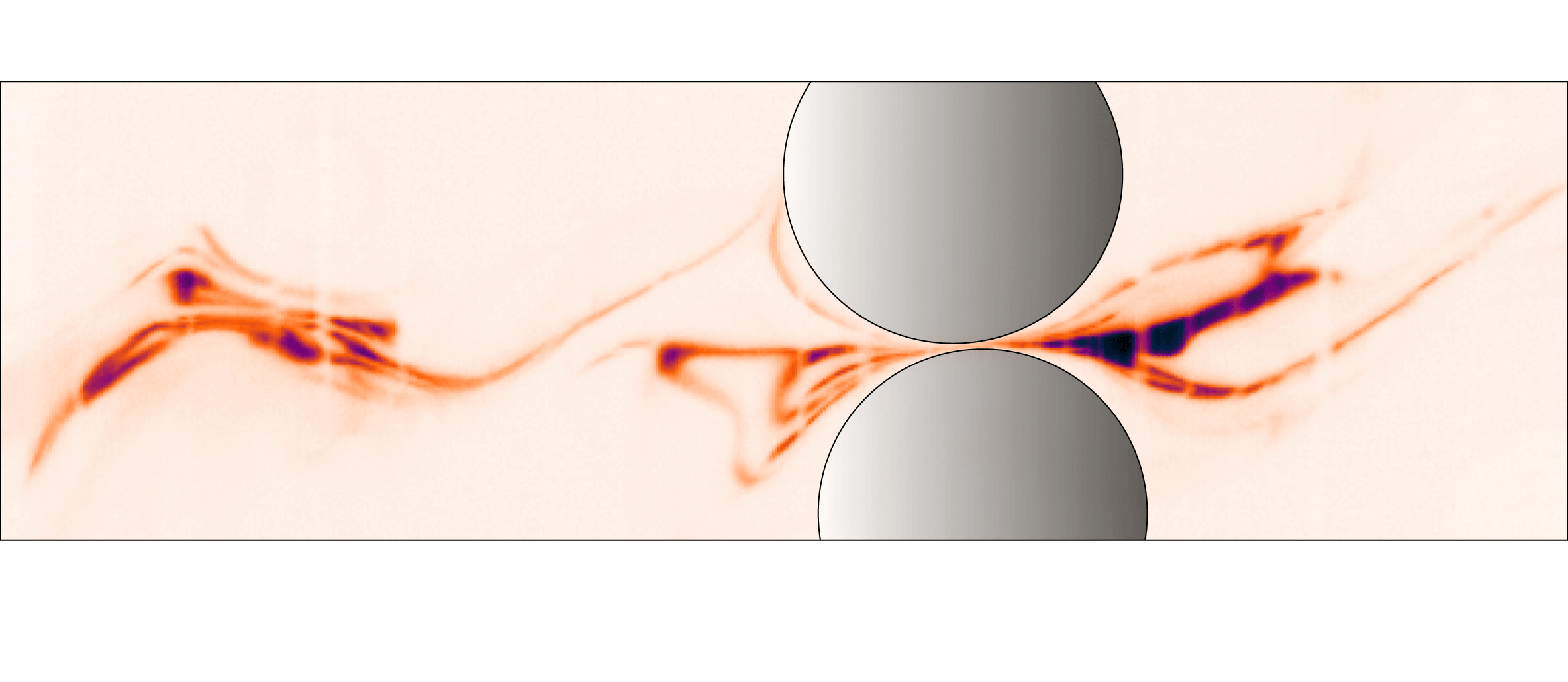
) and, from that instant of time, overlaps of the folded scalar filaments will be unavoidable. Such an event is illustrated in figure 16. These overlaps will locally delay the mixing process and therefore affect the whole route of the mixture towards homogenization. This aspect, and more generally all aspects regarding the concentration content of the mixture and its evolution, are left for future research.
Picture illustrating the complexity of folding of the stretched blob of dye and the potential interaction (merging) of nearby filaments.

7 Conclusions
Motivated by the need to understand on a firm basis the mixing properties of particulate flows, we have provided a complete characterization of the kinematics of stretchings and consecutive elongations of material lines in non-Brownian particulate suspensions under a simple macroscopic shear. Our observations rely on high-resolution PIV measurements of the interstitial fluid velocity field, and our findings are as follows.
-
(i) Following the Diffusive Strip Method of Meunier & Villermaux (Reference Meunier and Villermaux2010), we used the experimentally measured velocity fields to numerically advect passive segments in order to reconstruct the stretching histories of fluid material lines. In agreement with previous theoretical predictions and simulation results, we observe that adding particles in a shear flow changes the very nature of the stretching laws from linear to exponential in strain. The growth rate for the mean elongation are found to closely agree with the largest Lyapunov exponent obtained from 3D numerical simulations (Dasan et al. Reference Dasan, Ramamohan, Singh and Nott2002; Drazer et al. Reference Drazer, Koplik, Khusid and Acrivos2002). Besides the mean, our analysis also provides the full statistics of the material line elongation: the variances of the elongations also grow exponentially in strain and the distributions of elongations converge towards log-normals. This statistics of elongation was characterized for a large range of volume fractions
 $20\,\%\leqslant \unicode[STIX]{x1D719}\leqslant 55\,\%$
.
-
(ii) Using the same velocity fields, we determined the distribution of the local shear rate intensities and their persistence time. From these, we have shown how the fluid material lines undergo a multiplicative stretching process consisting in a noisy multiplicative sequence of correlated motions. We also discussed the important role of the finite correlation time of the velocity field. The model quantitatively predicts the evolution of the mean and the variance of the elongations of the fluid material lines as well as their evolution towards a log-normal distribution.
-
(iii) We have discussed the importance of this characterization of the flow kinematics to understand how mixing proceeds in sheared particulate suspensions. The exponential stretching results in a mixing time increasing logarithmically with the Péclet number. Moreover, the broad distribution of stretching rates implies a broad distribution of mixing times. The stochastic nature of the stretching process thus allows stretching rates that are smaller than in a pure shear flow. However, our analysis shows that the occurrence of such events becomes negligible at large Péclet number (
$\gg 10^{5}$
), as mixing occurs at larger deformations.


The present study opens the way for a complete description of the mixing process occurring in sheared particulate suspension. In particular, it allows the prediction of the evolution of the concentration distribution
 $P(C,t)$
(Duplat et al.
Reference Duplat, Innocenti and Villermaux2010). A quantitative verification of these predictions requires a specific experimental device that resolves the Batchelor scale
 $s(t_{mix})$
which corresponds to the transverse dimension of the filaments at the time when diffusion significantly modifies the concentration levels. Such challenging measurements will be addressed in future studies.
Acknowledgements
We would like to thank P. Meunier for letting us use his DSM code, S. Dagois Bohy, S. Gallier, E. DeGiuli, M. Wyart and O. Pouliquen for thoughtful discussions, and P. Cervetti, S. Noel and S. Martinez for helping us build the experimental set-up. This work was supported by ANR JCJC SIMI 9 and by the Labex MEC ANR-10-LABX-0092 et ANR-11-IDEX-0001-02.
Supplementary movies
Supplementary movies are available at https://doi.org/10.1017/jfm.2016.828.