1. Introduction
Richtmyer–Meshkov instability (RMI) (Richtmyer Reference Richtmyer1960; Meshkov Reference Meshkov1969) is a fundamental hydrodynamic instability that arises when a shock wave interacts with a perturbed interface separating two fluids with distinct densities. During the RMI evolution, the lighter fluid penetrates into the heavier fluid, forming bubble structures, while the heavier fluid intrudes into the lighter fluid, forming spike structures. As a foundation for RMI research, the instability on single-mode interfaces (single-mode RMI) has been the subject of extensive investigation (Brouillette Reference Brouillette2002; Zhou Reference Zhou2017a ,Reference Zhou b , Reference Zhou2024; Zhou et al. Reference Zhou2021). However, in engineering applications and natural phenomena involving RMI, such as inertial confinement fusion (ICF) (Zhou, Sadler & Hurricane Reference Zhou, Sadler and Hurricane2025) and supernova explosions (Abarzhi et al. Reference Abarzhi, Bhowmick, Naveh, Pandian, Swisher, Stellingwerf and Arnett2019), the instability is typically seeded by stochastic perturbations at material interfaces. Therefore, investigating the instability on multi-mode interfaces and elucidating the underlying mechanisms are crucial. Current studies of RMI on broadband or randomly perturbed interfaces predominantly rely on statistical methods to analyse spectral features associated with energy transfer (Dimonte et al. Reference Dimonte, Nagori, Ramaprabhu and Boureima2024; Zhou Reference Zhou2024; Zhao et al. Reference Zhao, Ding, He, Zhou and Luo2025). The inherent complexity of the initial perturbation spectrum in such configurations hinders elucidating the influence of higher-order initial modes on interface evolution (higher-order-mode effect). This challenge highlights the necessity for research into simpler interface configurations. Quasi-single-mode interfaces possess a dominant mode that preserves geometric regularity while simultaneously incorporating higher-order components. This feature makes the RMI at quasi-single-mode interfaces (quasi-single-mode RMI) a critical bridge connecting classical single-mode RMI and RMI on interfaces with stochastic perturbations, and a favourable subject for exploring the higher-order-mode effect on interface evolution.
Extensive experimental efforts have been devoted to examining the RMI on specific types of quasi-single-mode interfaces, with particular emphasis on the V-shaped interface evolution (Rikanati et al. Reference Rikanati, Oron, Sadot and Shvarts2003; Reilly et al. Reference Reilly, McFarland, Mohaghar and Ranjan2015; Luo et al. Reference Luo, Dong, Si and Zhai2016; Mohaghar et al. Reference Mohaghar, Carter, Musci, Reilly, McFarland and Ranjan2017, Reference Mohaghar, Carter, Pathikonda and Ranjan2019; Guo et al. Reference Guo, Zhai, Si and Luo2019). However, these studies primarily concerned the dependence of quasi-single-mode RMI on parameters such as the initial amplitude and shock strength, without exploring the higher-order-mode effect. To investigate the influence of higher-order initial modes, Bakhrakh et al. (Reference Bakhrakh, Klopov, Meshkov, Tolshmyakov and Yanikin1995) studied RMI at circular-arc, square-waveform and V-shaped interfaces subjected to a shock wave with Mach number
 $M_s=1.44$
, combining experimental and numerical approaches. They identified a strong correlation between the amplitude growth and the interface geometry. Liang et al. (Reference Liang, Zhai, Ding and Luo2019) further examined RMI on diverse quasi-single-mode interfaces, including circular-arc, V-shaped, trapezoidal and square-waveform geometries, accelerated by a shock with
 $M_s = 1.2$
. They demonstrated that the linear evolution of quasi-single-mode RMI differs from that of the single-mode case, with the deviation primarily governed by the Fourier expansion coefficient of the fundamental mode. Additionally, they developed an empirical nonlinear model based on the principle of linear superposition (Mikaelian Reference Mikaelian2005), which successfully reproduces the weakly nonlinear evolution of all the examined interfaces. Guo et al. (Reference Guo, Cong, Si and Luo2022) conducted experiments on RMI at single-mode, trapezoidal and V-shaped interfaces driven by a weak shock with
 $M_s = 1.3$
. They reported that the growth of the mixing width is strongly dependent on the initial interface profile. Specifically, the higher-order modes of the V-shaped interface are all in phase with the fundamental mode, and their contribution leads the V-shaped interface to evolve more rapidly than the others.
Notably, the experimental studies discussed above were performed exclusively in the weak-shock regime (
 $M_s \lt 2.0$
). However, in realistic scenarios such as ICF and supernova explosions, RMI is triggered by strong shock waves, which introduce significant compressibility, leading to an evolution law that markedly differs from that under weak-shock conditions (Zhou Reference Zhou2024; Si et al. Reference Si, Jiang, Cai, Wang and Luo2025). Consequently, the investigation of strong-shock-induced RMI is of considerable significance. While laser-driven experiments are capable of generating shock waves with
 $M_s$
up to 10 or even higher (Dimonte & Remington Reference Dimonte and Remington1993; Dimonte et al. Reference Dimonte, Frerking, Schneider and Remington1996; Glendinning et al. Reference Glendinning2003), they typically involve additional physicochemical processes such as material phase transitions and rarefaction-wave-induced decompression, which complicates isolating the contribution of RMI to perturbation growth. In contrast, shock-tube experiments offer a more controlled and simple physical environment for exploring the RMI dynamics. However, only a few shock-tube experiments on RMI with
 $M_s \geqslant 2.0$
have been reported (Ranjan et al. Reference Ranjan, Anderson, Oakley and Bonazza2005, Reference Ranjan, Niederhaus, Motl, Anderson, Oakley and Bonazza2007), primarily due to the difficulty in generating well-controlled strong shock waves in a shock-tube facility. To our knowledge, the only reported experiment on quasi-single-mode RMI with
 $M_s \geqslant 2.0$
was conducted by Sadot et al. (Reference Sadot, Rikanati, Oron, Ben-Dor and Shvarts2003). They employed a solid membrane with a support structure to separate gases, and investigated RMI at a V-shaped interface accelerated by a shock wave with
 $M_s = 2.0$
in a horizontal shock tube. Their results showed that the amplitude growth is inhibited under the influence of shock proximity and secondary compression. However, the support structure and membrane remnants could exert a significant influence on the perturbation evolution. Moreover, only a single interface configuration was considered, hindering the exploration of the higher-order-mode effect.
To date, desirable and systematic experimental research on quasi-single-mode RMI induced by strong shock waves remains lacking. The underlying evolution mechanisms, along with the applicability of existing models for instability characterisation, are unclear, motivating the present study. In our recent work (Jiang et al. Reference Jiang, Cai, Xie, He, Wang, Si and Luo2024), a shock-tube facility capable of producing shock waves with
 $M_s \gt 3.0$
while maintaining a ‘clean’ experimental flow was developed. Furthermore, a novel technique enabling the controllable generation of interfaces without support structures was proposed. These advancements offer a rare opportunity to explore the higher-order-mode effect under strong-shock conditions. In this work, one single-mode interface and four quasi-single-mode interfaces of varying initial modal compositions, including circular-arc, V-shaped, trapezoidal and square-waveform configurations, are considered to highlight the higher-order-mode effect. The morphological evolution of diverse interfaces is first discussed, followed by an analysis of their amplitude evolution dynamics.
2. Experimental methods and set-up
Given the pronounced sensitivity of RMI to initial conditions (Zhou Reference Zhou2024), a high-confidence experimental investigation of strong-shock-driven quasi-single-mode RMI necessitates two essential prerequisites: the generation of a high-intensity shock with a ‘clean’ post-shock flow field, and the formation of well-controlled initial interfaces.
In the present study, the incident shock with
 $M_s \gt 3.0$
and a ‘clean’ post-shock flow is generated using a recently developed shock-tube facility (Jiang et al. Reference Jiang, Cai, Xie, He, Wang, Si and Luo2024), the overall structure of which is illustrated in figure 1. The fundamental principle underlying this facility is that the shock intensity increases as the shock area decreases (Chester Reference Chester1954; Chisnell Reference Chisnell1957; Whitham Reference Whitham1957). The reduction in shock area is achieved through a convergence section specifically designed based on the geometrical shock dynamics (GSD) (Han & Yin Reference Han and Yin1993; Zhai et al. Reference Zhai, Liu, Qin, Yang and Luo2010; Zhan et al. Reference Zhan, Li, Yang, Zhu and Yang2018). During the convergence process, the cross-sectional area of the shock wave decreases from 120 mm
 $\times$
262 mm to 120 mm
 $\times$
8 mm, leading to an increase in
 $M_s$
from approximately 2.0 to over 3.0. In contrast to direct or abrupt shock-contraction approaches, which typically induce strong post-shock disturbances due to shock reflections (Russell Reference Russell1967), or empirical wall-profile design methods, which demand multiple iterations yet still fail to completely eliminate strong post-shock disturbances (Dowse & Skews Reference Dowse and Skews2014), the GSD-based design is capable of producing a stable shock accompanied by a ‘clean’ post-shock flow.
Sketch of the shock-tube facility capable of generating a planar shock with
 $M_s \gt 3.0$
while maintaining a ‘clean’ flow field.

Schematics of (a) interface formation method and (b) high-speed shadowgraph imaging system.

The initial interfaces are generated using the polyester-film technique developed specifically for strong-shock-driven RMI experiments (Jiang et al. Reference Jiang, Cai, Xie, He, Wang, Si and Luo2024; Cai et al. Reference Cai, Jiang, Wang, Wang, Ma and Si2025; Si et al. Reference Si, Jiang, Cai, Wang and Luo2025). The interface-formation devices (I and II), shown in figure 2(a), are fabricated by assembling transparent acrylic plates and pedestals, with the adjacent boundaries machined into the desired interface profile. The procedure for interface formation is as follows. Polyester films with thickness 2
 $\unicode {x03BC}$
m are first carefully attached to the upstream and downstream sides of device II using double-sided tape. To enable gas replacement in device II, two small holes are punctured in the downstream film, allowing the insertion of an inlet needle and an outlet pipe. Then SF
 $_6$
is injected through the inlet, while air is vented through the outlet. The exhausted gas is monitored using an oxygen concentration detector. Once the detected oxygen volume fraction drops below 0.3 %, the needle and pipe are removed, and the holes are subsequently sealed. Devices I and II are then carefully connected to form an air–SF
 $_6$
interface. The small height of the experimental channel (8 mm) ensures effective confinement of the interface by the upper and lower boundaries, thus eliminating the need for a support structure. Compared with the soap-film technique (Luo et al. Reference Luo, Dong, Si and Zhai2016; Liang et al. Reference Liang, Zhai, Ding and Luo2019), which can also produce initial interfaces without diffusion layer and support structure, the polyester-film technique possesses an additional advantage: a significantly longer maintainable duration. This advantage is particularly crucial for the present experiments, as the interval from gas filling to shock initiation is considerably longer than that in the weak-shock experiments.
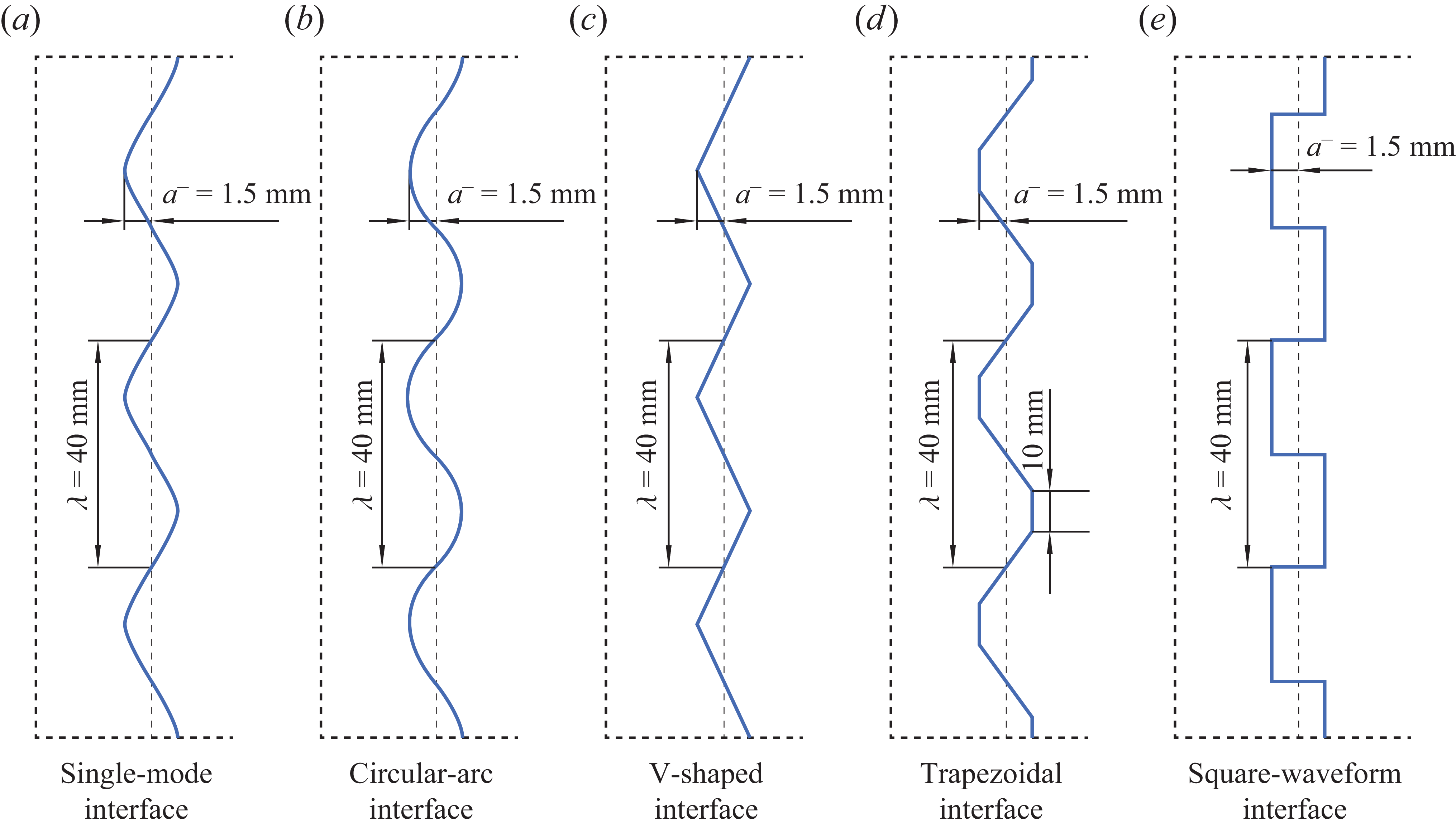
Schematics of initial interface configurations, where
 $a^-$
is initial amplitude, and
 $\lambda$
is perturbation wavelength.

Five distinct interface configurations, including the single-mode, circular-arc, V-shaped, trapezoidal and square-waveform geometries, are considered, with the corresponding profiles illustrated in figure 3. The perturbation wavelength (
 $\lambda$
) is fixed at 40 mm, and the scaled initial amplitude (
 $ka^-$
, where
 $k$
and
 $a^-$
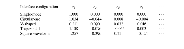
denote the perturbation wavenumber and initial amplitude, respectively) is set to 0.236 to minimise the potential influence of high initial amplitude on perturbation evolution. The trapezoidal interface is assigned base length 10 mm, representing a transitional form between the V-shaped and square-waveform interfaces, which can be considered as trapezoids with base lengths 0 and 20 mm, respectively. To quantify the differences in initial modal composition, the interface profiles are expanded in a Fourier series as
 $y = a^-\sum _i{c_i\cos(ikx)}$
, with the corresponding coefficients
 $c_i$
(
 $i = 1,2,3,\ldots$
) summarised in table 1. Notably, only the coefficients of the odd-order modes are listed, since those of the even-order modes vanish identically. For the circular-arc interface,
 $c_1$
is close to unity, and the absolute values of the coefficients for higher-order modes are small, suggesting that it deviates slightly from the single-mode interface. For the V-shaped interface, all coefficients share the same sign, with
 $c_1$
substantially smaller than unity. For the trapezoidal (square-waveform) interface,
 $c_1$
is slightly (significantly) greater than unity, and the absolute values of the coefficients for higher-order modes are relatively small (large). From the modal perspective, the circular-arc interface exhibits the smallest deviation from the single-mode configuration, whereas the square-waveform interface exhibits the largest deviation. By contrast, for the V-shaped and trapezoidal interfaces, the modal amplitudes do not provide a consistent indication of which interface deviates more markedly from the single-mode configuration. Notably, to assess the repeatability of the experiments, two separate runs have been conducted for each interface configuration. As shown in Appendix A, the key parameters of the repeated runs are in close agreement, confirming the repeatability of the experiments. For clarity, only the first run for each interface configuration is considered in the following discussion, and each case is designated according to the interface morphology.
Coefficients of initial modal components for single-mode and quasi-single-mode interfaces.

The flow field is illuminated using a light source (CEL-PF300-T10) and captured by a high-speed video camera (Phantom V2012) through a shadowgraph imaging system, as shown in figure 2(b). The camera operates at 100 000 frames per second with exposure time 1
 $\unicode {x03BC}$
s, yielding spatial resolution approximately 0.57 mm per pixel. The ambient pressure and temperature are 101.3
 $\pm$
0.8 kPa and 295.3
 $\pm$
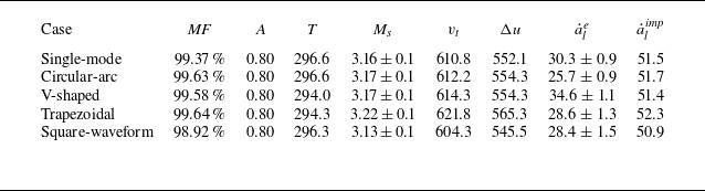
1.3 K, respectively. The gas upstream of the interface is considered to be pure air owing to the favourable sealing property of the polyester film, and the downstream gas component is determined by matching the velocity of the transmitted shock measured experimentally with that predicted using the one-dimensional gas dynamics theory. Key experimental parameters for the five experiments, including the mass fraction of
 $\mathrm{SF_6}$
downstream of the initial interface (
 $\textit{MF}$
), post-shock Atwood number (
 $A$
), velocity of the transmitted shock (
 $v_t$
) and interface jump velocity (
 $\Delta u$
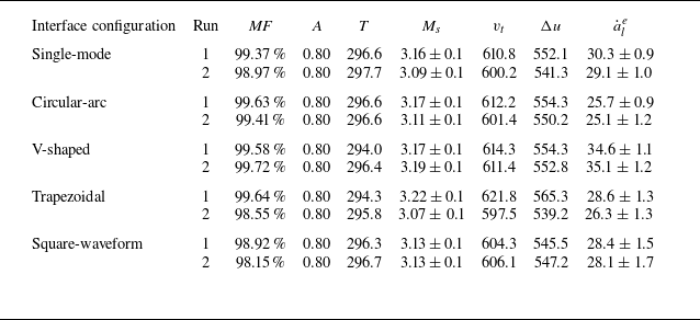
), are summarised in table 2. The close agreement of these parameters across different experiments further demonstrates the high experimental reproducibility. Moreover, to assess the reliability of the experimental measurements, Appendix A presents a discussion of the measurement uncertainties in interface amplitude, linear amplitude growth rate, and
 $M_s$
. These analyses, together with the quantitative results presented in table 2 and figures 6–10, confirm the reliability of the experimental measurements.
Significant parameters for five experiments with various initial interface configurations:
 $ \textit{MF}$
is the mass fraction of
 $\mathrm{SF_6}$
downstream of the initial interface;
 $A = (\rho _2 - \rho _1)/(\rho _2 + \rho _1)$
is the post-shock Atwood number, with
 $\rho _1$
and
 $\rho _2$
denoting the densities of gases upstream and downstream of the post-shock interface, respectively;
 $T$
is the ambient temperature;
 $M_s$
is the Mach number of the incident shock;
 $v_t$
is the velocity of the transmitted shock;
 $\Delta u$
is the interface velocity jump;
 $\dot {a}_{l}^{e}$
and
 $\dot {a}_{l}^{\textit{imp}}$
are the linear amplitude growth rates obtained from experiments and predicted by the impulsive model, respectively. Units of parameters representing velocity (or amplitude growth rate) and temperature are m s−1 and K, respectively.

3. Flow features under strong-shock conditions
The experimental shadowgraph images of the evolution of single-mode and quasi-single-mode interfaces accelerated by a strong shock wave are presented in figure 4. The temporal origin (
 $t = 0$
 $\unicode {x03BC}$
s) is defined as the moment when the incident shock reaches the mean position of the initial interface. For clarity, the shadows caused by the device edges, which convey no flow information, are removed from the images through post-processing after the shocks and interface have separated from them. It is noteworthy that the observed physical areas are slightly different from run to run, which constitutes the primary reason why the interface displacement trends among different cases in figure 4 are not completely consistent with the quantitative
 $\Delta u$
values listed in table 2. Owing to the high shock intensity involved in the present experiments, mechanical vibrations generated during shock propagation through the shock tube can induce slight shifts in the shadowgraph optical path from run to run. Nevertheless, this does not compromise the quantitative analysis, because all parameters for each individual run are extracted based on its corresponding observed area. Specifically, the spatial calibration for each run is performed independently using an identical optical set-up and the same calibration procedure, thereby ensuring that the measured data remain directly comparable across different cases.
Experimental shadowgraphs of the evolution of single-mode and quasi-single-mode interfaces accelerated by strong shock waves: (a) single-mode interface; (b) circular-arc interface; (c) V-shaped interface; (d) trapezoidal interface; (e) square-waveform interface. Here,
 $a$
is interface amplitude, and numbers represent the time in
 $\unicode {x03BC}\mathrm{s}$
.

In the single-mode case, which serves as a reference for the quasi-single-mode scenarios, the reflected and transmitted shocks are generated when the incident shock impacts the initial interface. The reflected shock propagates downstream because the Mach number of the flow ahead (up to 1.4) exceeds its own Mach number (1.3). This behaviour is consistent with the theoretical analysis of Mikaelian (Reference Mikaelian2016), which demonstrates that the reflected shock propagates downstream for flows initiated by an incident shock with
 $M_s \gt 2.76$
, and upstream for that with
 $M_s \lt 2.76$
, with
 $M_s = 2.76$
corresponding to the special case of a standing shock at rest. At early times (
 $t \lt 10$
 $\unicode {x03BC}$
s), the reflected shock overlaps the shadows from the device edges, while the transmitted shock remains close to the shocked interface, making them indistinguishable. Notably, the relative separation velocity of the transmitted shock from the shocked interface, defined as (
 $v_{t}-\Delta u)/v_{t}$
, in the present experiments (
 $\sim0.095$
) is significantly lower than that under weak-shock conditions reported by Liang et al. (Reference Liang, Zhai, Ding and Luo2019) (
 $\sim0.62$
). Shortly after these discontinuities become distinguishable, distinct spike and bubble structures emerge (
 $t = 70$
 $\unicode {x03BC}$
s). Owing to the compressibility effects introduced by the strong shock wave (Si et al. Reference Si, Jiang, Cai, Wang and Luo2025), the bubble front remains significantly flatter than that under weak-shock conditions (Li et al. Reference Li, Cao, Wang, Zhai and Luo2023) throughout the evolution process.
The circular-arc interface exhibits evolution closely resembling that of the single-mode interface, due to only slight differences in modal composition. In contrast, other quasi-single-mode interfaces exhibit significant morphological deviations relative to the single-mode interface. For the V-shaped case, during the early stage (
 $t \lt 103$
 $\unicode {x03BC}$
s), the tips of the bubble and spike are sharper than in the single-mode case, accompanied by the emergence of small concave structures in between. Subsequently, these concave structures vanish gradually and the bubble flattens. The spike remains sharp until the intermediate stage (133
 $\unicode {x03BC}$
s), yet ultimately evolves towards the late-stage morphology of the single-mode interface (233
 $\unicode {x03BC}$
s).
For the trapezoidal and square-waveform cases, a cavity emerges at the spike tip in the early period. This phenomenon results from a vortex pair arising from strong vorticity deposited at the upstream corners during shock impact, which initially rolls up upstream, as illustrated in figure 5(a). In particular, in the square-waveform case, where the upstream corners are sharper than those in the trapezoidal case, a pronounced vortex pair and cavity form at a very early stage (10–30
 $\unicode {x03BC}$
s). As the interface evolves, the cavity progressively vanishes under the action of the vortex-pair-induced velocity field, which directs upstream at the spike tip, as sketched in figure 5(b). At the upper (lower) junction of the spike and bubble, the perturbed velocity field directs upwards (downwards), thereby driving the expansion of the bubble front and narrowing of the spike stem. In the square-waveform case, the strong vortex pair drives the portion of the interface between the bubble tip and spike–bubble junction downstream more rapidly than the bubble tip itself, producing a concave bubble tip throughout the evolution. In contrast, the comparatively weaker vortex pair in the trapezoidal case induces only a slight concavity at the bubble tip during the intermediate stage (
 $\sim69{-}129$
 $\unicode {x03BC}$
s).
Sketches of the shock waves and interface morphology at the early and late stages for trapezoidal and square-waveform cases, along with the perturbed velocity field in the region behind the transmitted shock, obtained by subtracting the background one-dimensional velocity in the area between transmitted and reflected shocks from the particle velocity field. The colour of the arrow represents the magnitude of the velocity: the darker the colour, the greater the velocity. Red, blue and black lines denote the shocked interface, transmitted shock and transverse wave, respectively.

4. Amplitude evolution in highly compressible flow
In this study, following the convention in RMI studies (Zhou et al. Reference Zhou2021; Zhou Reference Zhou2024), the overall interface amplitude (
 $a$
) is defined as
 $(|a_b| + |a_s|)/2$
, where
 $a_b$
and
 $a_s$
denote the bubble and spike amplitudes, respectively. Specifically,
 $a_b$
(
 $a_s$
) is defined as the streamwise coordinate difference between the bubble (spike) tip and the mean interface position. At the early time, the experimental
 $a_{b/s}$
and the interface velocity jump
 $\Delta u$
are determined according to the mean positions of the shocked interface obtained via Fourier analysis. A detailed description of the Fourier-based data processing procedure can be found in Appendix B. At later stages, however, when vortex roll-up becomes significant, the interface can no longer be accurately described as a single-valued function. Under such conditions, the Fourier-based method is no longer reliable and may introduce significant errors. Consequently, the mean interface position is no longer directly determined from the interface contour. Instead, it is obtained by extrapolating the mean interface positions determined at the earlier time based on
 $\Delta u$
, thereby enabling the determination of
 $a_{b}$
and
 $a_{s}$
throughout the entire interface evolution.
The amplitude evolution typically proceeds through three successive stages: start-up, linear and nonlinear (Zhou Reference Zhou2024). In the start-up stage (Lombardini & Pullin Reference Lombardini and Pullin2009), the amplitude growth rate (
 $\dot {a}$
) rises from zero and gradually reaches an asymptotic value (
 $\dot {a}_l$
) under the drive of pressure perturbations. Afterwards,
 $\dot {a}$
remains approximately constant over a period known as the linear stage. As the flow evolves further and nonlinearity becomes pronounced,
 $\dot {a}$
decreases, marking the onset of the nonlinear evolution stage.
4.1. Start-up to linear evolution stages
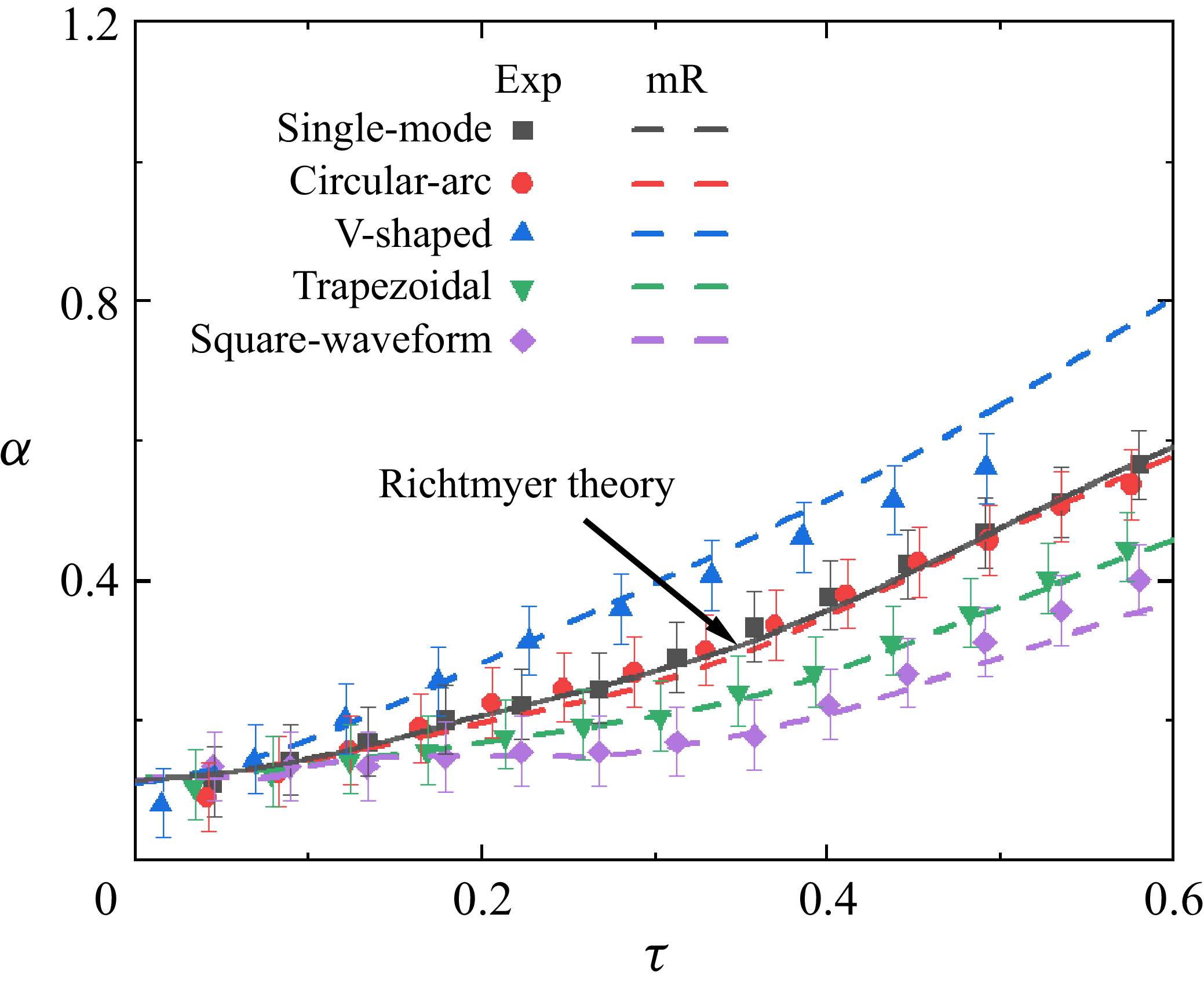
The amplitude evolution of different interfaces from the start-up stage to the linear stage is presented in figure 6 in dimensionless form. Here,
 $t$
and
 $a$
are normalised to
 $\tau = k \dot {a}_{l}^et$
and
 $\alpha = ka$
, respectively, where
 $\dot {a}_l^e$
represents the experimental
 $\dot {a}_l$
. For the single-mode, circular-arc, trapezoidal and square-waveform cases,
 $\dot {a}$
increases until
 $\tau \approx 0.38$
, after which it remains nearly constant until
 $\tau \approx 0.57$
. In contrast,
 $\dot {a}$
for the V-shaped interface rapidly reaches its peak value, after which it remains nearly constant until
 $\tau \approx 0.49$
. The earlier onset of the nonlinear regime for the V-shaped interface is attributed to its modal composition. The V-shaped interface contains exclusively positive higher-order Fourier modes, thereby leading to a more rapid evolution at the early time compared with the single-mode interface and other quasi-single-mode interfaces containing both positive and negative modes (Liang et al. Reference Liang, Zhai, Ding and Luo2019; Guo et al. Reference Guo, Cong, Si and Luo2022). As a result, the linear regime of the V-shaped interface ends earlier.
Dimensionless amplitude evolution of single-mode and quasi-single-mode interfaces from the start-up to linear stages. Symbols indicate experimental data; solid and dashed lines indicate predictions from Richtmyer theory and the mR model, respectively, where the mR model denotes the model obtained by extending the Richtmyer theory through linear superposition. Note that the predictions of the Richtmyer theory and mR model coincide for the single-mode case.

The classical linear model proposed by Richtmyer (Reference Richtmyer1960) (impulsive model), which has been validated for weak-shock-driven single-mode RMI (Chen et al. Reference Chen, Xing, Wang, Zhai and Luo2023), is first considered as a theoretical reference for comparison with the experiments. The model can be expressed as
 \begin{align} \dot {a}_{l}^{\textit{imp}} = k\,\Delta u\,A a^+. \end{align}
Here,
 $a^+ = a^-(1-\Delta u/v_{is})$
represents the post-shock amplitude, where
 $v_{is}$
denotes the incident shock velocity. It is worth noting that for the quasi-single-mode interfaces, the amplitude adopted for prediction is also the overall initial interface amplitude
 $a^-$
, i.e. the amplitude resulting from the superposition of all Fourier modes, rather than the amplitude of the fundamental Fourier component alone. This choice is made for comparative purposes, allowing the influence of higher-order modes to be evaluated indirectly by comparing
 $ \dot {a}_{l}^{e}$
and
 $\dot {a}_{l}^{\textit{imp}}$
across different interface configurations (Liang et al. Reference Liang, Zhai, Ding and Luo2019). Moreover, the minor differences in
 $\dot {a}_{l}^{\textit{imp}}$
reported in table 2 are due to slight variations in the initial flow conditions rather than differences in the computational procedure. The comparison between
 $\dot {a}_{l}^{e}$
and
 $\dot {a}_{l}^{\textit{imp}}$
indicates that higher-order modes influence the linear evolution, and the impulsive model fails to accurately predict
 $\dot {a}_{l}^{e}$
even for the single-mode case. This failure stems from the inadequacy of the model’s empirical correction – i.e. using
 $a^+$
and
 $A$
instead of the pre-shock counterparts for prediction – in capturing the influence of compressibility on interface evolution in highly compressible flow (Mikaelian Reference Mikaelian1994; Yang, Zhang & Sharp Reference Yang, Zhang and Sharp1994; Wouchuk Reference Wouchuk2001; Napieralski et al. Reference Napieralski, Cobos, Velikovich and Huete2024; Si et al. Reference Si, Jiang, Cai, Wang and Luo2025).
In addition to the impulsive model, Richtmyer (Reference Richtmyer1960) also proposed a compressible linear theory (Richtmyer theory) that is theoretically valid for strongly compressible flows. As shown in figure 6, the Richtmyer theory effectively captures the early-time amplitude evolution of the single-mode RMI. Notably, although previous work (Si et al. Reference Si, Jiang, Cai, Wang and Luo2025) experimentally verified its capability to predict
 $\dot {a}_{l}$
under highly compressible conditions, the present study provides the first experimental evidence supporting its applicability in describing the strong-shock-driven single-mode RMI evolution from the start-up to linear stages. In contrast, this theory underestimates the early-time evolution of the V-shaped interface, and overestimates the growth of the circular-arc, trapezoidal and square-waveform interfaces. This highlights that higher-order modes play a significant role in the early-time evolution of quasi-single-mode interfaces, and must be taken into account.
Assuming that the amplitude evolution of a quasi-single-mode interface is the linear superposition of the growth of each initial mode (Mikaelian Reference Mikaelian2005), and that the contribution of harmonic modes (i.e. modal components arising from coupling) is negligible, a linear model for quasi-single-mode RMI (referred to as the mR model) is constructed as follows:
 \begin{align} \dot {a}^{\textit{mR}}(t) & = \sum _i{c_i\,\dot {a}^{R}_i(t)},\quad i = 1,2,3,\ldots , \nonumber \\[3pt] a^{\textit{mR}} & = \int {\dot {a}^{\textit{mR}}}\,{\rm d}t =\int {\sum _i{c_i\dot {a}^{R}_i}\,{\rm d}t} \nonumber \\[3pt] & = \sum _i{c_i\,a^{R}_i(t)},\quad i = 1,2,3,\ldots . \end{align}
Here,
 $\dot {a}^{R}_i$
and
 $a^{R}_i$
represent the amplitude growth rate and amplitude predicted by the Richtmyer theory for the
 $i$
th-order initial mode with initial amplitude
 $a^-$
, respectively. The predictions of the mR model for all cases are plotted in figure 6. It is noteworthy that the predictions of the mR model and the Richtmyer theory for the single-mode case are identical. The mR model provides a reasonable prediction of the experimental amplitude evolution from the start-up to the linear stages across all cases. These results indicate the validity of the assumptions underlying the mR model, i.e. the early-time evolution of quasi-single-mode RMI can be regarded as the linear superposition of the growth of each initial mode, with modal coupling remaining negligible.
4.2. Nonlinear evolution period
The temporal evolutions of
 $a$
and
 $a_{b/s}$
are presented in figures 7(a) and 7(b), respectively, in dimensionless form. Here,
 $t$
,
 $a$
and
 $a_{b/s}$
are normalised as
 $\tau = k \dot {a}_{l}^e (t - t^m)$
,
 $\alpha = k(a - a^m)$
and
 $\alpha _{b/s} = k(a_{b/s} - a^m_{b/s})$
, respectively, where
 $t^m$
represents the moment when
 $\dot {a}$
reaches
 $\dot {a}_{l}^e$
, and
 $a^m$
(
 $a^m_{b/s}$
) corresponds to the value of
 $a$
(
 $a_{b/s}$
) at
 $t = t^m$
. It is observed that the overall amplitude evolutions for the five experimental cases nearly collapse together, showing partial discrepancy with the findings of Liang et al. (Reference Liang, Zhai, Ding and Luo2019): the dimensionless amplitude growths of the single-mode, circular-arc, trapezoidal and square-waveform interfaces are similar, yet lower than that of the V-shaped interface. This discrepancy can be attributed to the pronounced compressibility effects, including the shock-proximity effect (Rikanati et al. Reference Rikanati, Oron, Sadot and Shvarts2003) and the associated influence of transverse waves, propagating in the region between the transmitted shock and shocked interface, on interface evolution (i.e. the secondary-compression effect) (Si et al. Reference Si, Jiang, Cai, Wang and Luo2025). Notably, these effects are more pronounced when the interface is located closer to the transmitted shock. As illustrated in figure 6, the V-shaped interface evolves considerably faster than the others in the early periods, bringing the bubble closer to the transmitted shock. As a result, the V-shaped interface experiences stronger compressibility-induced suppression on the evolution at later times, offsetting its initially faster growth, and yielding a final amplitude comparable to amplitudes of the others.
Concerning the amplitude growth of the bubble and spike, the square-waveform interface exhibits certain differences in evolution rate relative to the other interface configurations. Its slow bubble development arises from the initially flat front, whereas its rapid spike evolution is driven by the strong vortex pair, which promotes the upward motion of the spike tip. The other quasi-single-mode interfaces also exhibit distinct bubble and spike evolution rates relative to the single-mode interface. However, as their modal compositions are closer to the single-mode case compared with the square-waveform interface, the resulting differences in amplitude evolution are relatively minor. The nonlinear model proposed by Zhang & Guo (Reference Zhang and Guo2016) (the ZG model), which has been validated for weak-shock-driven RMI at a single-mode air–SF
 $_6$
interface (Chen et al. Reference Chen, Xing, Wang, Zhai and Luo2023), is considered here as a theoretical reference. The ZG model can be expressed as
 \begin{align} \dot {a}_{b/s}^{ZG} = \frac {\dot {a}_l^e}{1+\xi _{b/s}k\dot {a}_l^et}, \end{align}
where
 \begin{align} \xi _{b/s} = \frac {3}{4}\frac {(1 \pm \lvert A \rvert )(3 \pm \lvert A \rvert )}{3 \pm \lvert A \rvert + \sqrt {2(1 \pm \lvert A \rvert )}}\frac {4(3 \pm \lvert A \rvert )+\sqrt {2}(9 \pm \lvert A \rvert )(1 \pm \lvert A \rvert )^{{1}/{2}}}{(3 \pm \lvert A \rvert )^2 + 2\sqrt {2}(3 \mp \lvert A \rvert )(1\pm \lvert A \rvert )^{{1}/{2}}}, \end{align}
with the
 $+$
and
 $-$
signs referring to the bubble and spike, respectively. For the present experiments with
 $A=0.8$
, we have
 $\xi _{b} = 1.34$
and
 $\xi _{s} = 0.17$
. The predictions of the ZG model are presented in figure 7 for comparison. The model appears to reproduce the overall amplitude growth reasonably well, which, however, is a coincidence arising from the simultaneous overestimation of the bubble growth and underestimation of the spike evolution. Moreover, its predictive performance for the square-waveform case is particularly poor.
Temporal amplitude variations obtained from experiments (symbols) and predicted by the ZG model (dashed lines): (a) overall interface; (b) bubble and spike.

The failure of the ZG model in describing the present strong-shock experiments can be traced to three physical mechanisms that exert significant influences yet were not incorporated. First, compressibility effects, including the shock proximity and secondary compression: for the shock-proximity effect, the transmitted shock travels at a velocity comparable to the interface and stays near it for a prolonged period under strong-shock conditions, which was first pointed out by Mikaelian (Reference Mikaelian1994) and also discussed in Mikaelian (Reference Mikaelian2016). The interface is unable to penetrate the shock front, thus the evolution of the downstream interface structure (i.e. bubble for the light–heavy interface considered here) is significantly suppressed (Rikanati et al. Reference Rikanati, Oron, Sadot and Shvarts2003; Sadot et al. Reference Sadot, Rikanati, Oron, Ben-Dor and Shvarts2003). For the secondary-compression effect, the interaction between the incident shock and the disturbed interface produces a perturbed transmitted shock that subsequently develops into a Mach reflection with accompanying transverse waves. These transverse waves introduce pressure fluctuations in the vicinity of the interface, which further affect the interface evolution (Sadot et al. Reference Sadot, Rikanati, Oron, Ben-Dor and Shvarts2003; Guo et al. Reference Guo, Zhai, Ding, Si and Luo2020). Second, the spike-acceleration effect: at high
 $A$
, higher-order harmonic modes progressively concentrate at the spike tip and promote the spike growth (Dimonte & Ramaprabhu Reference Dimonte and Ramaprabhu2010; Chen et al. Reference Chen, Xing, Wang, Zhai and Luo2023; Si et al. Reference Si, Jiang, Cai, Wang and Luo2025). Third, the higher-order-mode effect arises from the presence of additional initial modes. The ZG model was originally developed for single-mode RMI, and the higher-order initial modes, which are intrinsic to quasi-single-mode RMI and affect both the bubble and spike evolution (Liang et al. Reference Liang, Zhai, Ding and Luo2019), were not considered.
The preceding analysis indicates that an effective model for describing the evolution of strong-shock-driven quasi-single-mode RMI must incorporate the coupled influences of the higher-order modes, shock proximity, secondary compression and spike acceleration. Developing such a model from first principles is highly challenging. Here, we propose an empirical extension of the ZG model, referred to as the
 $\varepsilon$
-ZG model, which is formulated as
 \begin{align} \dot {a}_{b}^{\varepsilon ZG} = \frac {\dot {a}_{l}^e}{1+\xi _{b}^{\varepsilon ZG}k\dot {a}_l^et}, \\[-28pt] \nonumber \end{align}
 \begin{align} \dot {a}_{s}^{\varepsilon ZG} = \frac {H_s\dot {a}_{l}^e}{1+\xi _{s}k\dot {a}_l^et+H_s(k\dot {a}_l^et)^2}, \\[0pt] \nonumber \end{align}
in which
 \begin{align} \xi _{b}^{\varepsilon ZG} &= F_{b}\xi _{b} + G_{b}, \nonumber \\[3pt]F_b(\varepsilon ) &= 1 - 20\varepsilon , \nonumber \\[3pt]G_b(\varepsilon , M_s) &= 1.5(\varepsilon +1)(M_s-1)\,{\rm e}^{-5k\dot {a}_l^et},\nonumber \\[3pt]H_s(\varepsilon , A) &= 1+A-\varepsilon ,\nonumber \\[3pt]\varepsilon & = \frac {c_3}{c_1+c_3}. \end{align}
The
 $\varepsilon$
-ZG model is formulated by incorporating the effects of the higher-order modes, shock proximity, secondary compression and spike acceleration into the framework of the ZG model in an empirical yet physically guided manner. For the higher-order-mode effect, which influences both the bubble and spike evolution, a coefficient
 $\varepsilon$
– i.e. the ratio of the third-order modal coefficient to the sum of the first- and third-order modal coefficients – is introduced to provide a simplified characterisation: Fourier analysis shows that the coefficients of the first- and third-order modes constitute the majority of the total modal amplitude, while those of higher-order modes contribute only marginally. For the bubble evolution, two dominant physical mechanisms are identified based on the present experiments: first, the higher-order-mode effect, which acts continuously throughout the evolution; second, compressibility effects, including shock proximity and secondary compression. These two effects are incorporated into the modified framework through the term
 $\xi _{b}^{\varepsilon ZG} = F_{b}\xi _{b} + G_{b}$
. The factor
 $F_b$
, including
 $\varepsilon$
, represents the continuous influence of the higher-order-mode effect, while
 $G_b$
primarily accounts for the suppression arising from compressibility effects. We formulate
 $G_b$
as a time-decaying function to represent the gradual attenuation of compressibility effects as the transmitted shock separates from the interface. For the spike evolution, two dominant physical effects are similarly identified based on the present experiments: first, the higher-order-mode effect acting continuously throughout the evolution; second, the spike-acceleration effect, which is associated with the progressive accumulation of harmonic modes near the spike tip during evolution. These two effects are incorporated into the modified framework through the coefficient
 $H_s$
, which incorporates both
 $\varepsilon$
, characterising the higher-order-mode effect, and
 $A$
, representing the spike-acceleration effect. Here,
 $H_s$
appears in both
 $H_s\dot {a}_l^e$
and
 $H_s(k\dot {a}_l^e t)^2$
:
 $H_s\dot {a}_l^e$
represents the influence of the two effects on the initial spike growth, while
 $H_s(k\dot {a}_l^e t)^2$
accounts for their continued contributions during subsequent spike evolution.
The predictions of the
 $\varepsilon$
-ZG model are presented in figure 8, demonstrating that it successfully captures the amplitude evolution of the overall interface, bubble and spike across all cases.
Temporal amplitude variations obtained from experiments (symbols) and predicted by the
 $\varepsilon$
-ZG model (dash-dotted line): (a) overall interface; (b) bubble and spike.

4.3. Complete amplitude evolution from start-up to nonlinear phases
In the quantitative analysis presented above, two new models, i.e. the mR and
 $\varepsilon$
-ZG models, have been developed to describe the amplitude evolution during the start-up-to-linear and nonlinear stages, respectively. Although each model reasonably captures the RMI evolution in the corresponding period, a theoretical framework that describes the complete amplitude evolution from the early start-up to the late nonlinear stage is more desirable. To achieve this, we employ a matching strategy to bridge the linear and nonlinear models describing the interface evolution. However, a key issue concerns where these two models should be connected, i.e. when the perturbation evolution can be considered to transition from the linear regime to the nonlinear regime. In the start-up period,
 $\dot {a}$
gradually approaches
 $\dot {a}_l^e$
, while nonlinearity may already emerge at this early stage. However, provided that
 $ka^-$
is small, the influence of nonlinearity on amplitude evolution could remain limited during the start-up period and for some time thereafter. Within this subsequent period, the amplitude evolution can still be approximated as linear, thus it is referred to as the linear stage (Wouchuk Reference Wouchuk2001). When nonlinearity becomes apparent and
 $\dot {a}$
falls below
 $\dot {a}_l^e$
, the amplitude evolution is considered to enter the nonlinear stage (Dimonte & Ramaprabhu Reference Dimonte and Ramaprabhu2010; Zhang & Guo Reference Zhang and Guo2016). Notably, the linear stage is an approximate description of a period where nonlinearity may exist but remains limited, i.e. linear amplitude evolution does not necessarily imply a strictly linear physical process. Consequently, it is challenging to rigorously define the demarcation point of the so-called linear stage from the nonlinear stage. In the present work, the end of the start-up period, i.e. the moment at which
 $\dot {a}$
first reaches
 $\dot {a}_l^e$
(
 $t^m$
), is taken as the transition point separating the linear and nonlinear physical processes, as well as the boundary between the regimes represented by the mR and
 $\varepsilon$
-ZG models. The matched model is formulated as
 \begin{align} \dot {a}^{\textit{match}}(t) = \begin{cases} \dot {a}^{\textit{mR}}(t), & t \leqslant t^m, \\[1ex] \dot {a}^{\varepsilon ZG}(t-t^m), & t \gt t^m. \end{cases} \end{align}
Here,
 $a^{\textit{match}}(0) = a^+$
and
 $\dot a^{\varepsilon ZG}(t) = [\dot a^{\varepsilon ZG}_b(t)+\dot a^{\varepsilon ZG}_s(t)]/2$
. The complete amplitude evolution can then be obtained by integrating
 $\dot a^{{match}}(t)$
over time. It should be emphasised that the matched model does not imply an abrupt physical transition, but instead establishes a continuous connection between the linear solution and the nonlinear evolution law.
Comparison of the experimental measurements and matched model predictions for the complete amplitude evolution from the early-time start-up to the late-time nonlinear stage.

The predictions of the matched model are presented in figure 9 alongside the experimental data for comparison. The results demonstrate that the model provides a reasonable prediction for the complete amplitude evolution of all five experiments. To further evaluate the matched model, the experimentally measured and theoretically predicted dimensional evolutions of
 $a_b$
and
 $a_s$
are presented in figures 10(a) and 10(b), respectively. The matched model reasonably predicts the bubble and spike amplitude evolutions individually. This indicates that the favourable agreement observed in figure 9 does not arise from compensating errors but instead reflects the model’s capability to describe both components separately.
Comparison of the experimental measurements and matched model predictions for the amplitude evolution of (a) the bubble and (b) the spike from the early-time start-up to the late-time nonlinear stage.

The above comparison indicates that although the interface evolution under strong-shock conditions differs from the weak-shock scenario, where the amplitude growth can be simply divided into a linear compressible stage followed by a nonlinear incompressible stage (Zhang & Sohn Reference Zhang and Sohn1997), the idea of modelling the complete amplitude evolution through matching the linear and nonlinear solutions remains applicable. This offers some insights for the future development of models for strong-shock-driven RMI.
4.4. Comparison between quasi-single-mode RMI in weak- and strong-shock regimes
To elucidate the differences in the evolution mechanisms between quasi-single-mode RMI under weak- and strong-shock conditions, it is instructive to compare the present findings with those reported in previous studies on weak-shock-induced quasi-single-mode RMI (Bakhrakh et al. Reference Bakhrakh, Klopov, Meshkov, Tolshmyakov and Yanikin1995; Liang et al. Reference Liang, Zhai, Ding and Luo2019; Guo et al. Reference Guo, Cong, Si and Luo2022). Notably, the interface configurations considered by Liang et al. (Reference Liang, Zhai, Ding and Luo2019) and in the present study are identical. Accordingly, the results of Liang et al. (Reference Liang, Zhai, Ding and Luo2019) are regarded as representative of quasi-single-mode RMI under weak-shock conditions, and are used for direct comparison with the present results.
Regarding the linear stage, Liang et al. (Reference Liang, Zhai, Ding and Luo2019) reported that the impulsive model accurately describes single-mode RMI under weak-shock conditions. For quasi-single-mode interfaces,
 $\dot {a}_{l}^{e}$
deviates from
 $\dot {a}_{l}^{\textit{imp}}$
as the interface deviates from a single-mode configuration, indicating that higher-order initial modes significantly affect the linear evolution (Liang et al. Reference Liang, Zhai, Ding and Luo2019). In the present strong-shock experiments, the impulsive model cannot describe the early-time dynamics of the single-mode interface well, because it fails to adequately account for flow compressibility (Mikaelian Reference Mikaelian1994; Yang et al. Reference Yang, Zhang and Sharp1994; Wouchuk Reference Wouchuk2001; Napieralski et al. Reference Napieralski, Cobos, Velikovich and Huete2024; Si et al. Reference Si, Jiang, Cai, Wang and Luo2025). In contrast, the compressible linear theory provides an accurate description of the single-mode case. For quasi-single-mode interfaces, higher-order initial modes likewise influence the early-time evolution, and their effects can be incorporated via linear superposition within the framework of the compressible linear theory.
Regarding the nonlinear stage, Liang et al. (Reference Liang, Zhai, Ding and Luo2019) reported that weak-shock-induced single-mode RMI can be accurately described by the ZG model, while the quasi-single-mode cases can be described by extending the ZG model through linear superposition of the contributions from individual modes. The validity of this superposition-based approach suggests that modal coupling remains weak, and that the nonlinear quasi-single-mode interface evolution is governed by the intrinsic nonlinearity captured by the ZG model, together with contributions from higher-order initial modes. Under strong-shock conditions, modal coupling also remains weak. However, in addition to intrinsic nonlinearity and the influence of higher-order initial modes, compressibility effects, including shock proximity and secondary compression, additionally affect the evolution law.
In summary, higher-order modes influence the linear and nonlinear evolution under both weak- and strong-shock conditions. The primary distinction between the two regimes lies in the degree of the compressibility, which leads to differences in the evolution characteristics and in the predictive performance of the corresponding models.
5. Conclusions
This study experimentally investigates the strong-shock-driven Richtmyer–Meshkov instability (RMI) at quasi-single-mode interfaces employing a novel shock-tube facility combined with an advanced interface-generation technique, with the incident shock Mach number reaching 3.18
 $\pm$
0.05. One canonical single-mode and four quasi-single-mode configurations, including the circular-arc, V-shaped, trapezoidal and square-waveform geometries, are considered to evaluate the influence of higher-order initial modes on instability evolution under strong-shock conditions.
Among the quasi-single-mode interfaces, the circular-arc interface exhibits only minor deviations in morphological evolution from the single-mode case, because they share nearly identical modal compositions. In contrast, the V-shaped, trapezoidal and square-waveform interfaces manifest markedly different evolution features. Specifically, the V-shaped interface preserves a sharp spike/bubble until the intermediate stage, yet ultimately tends towards the single-mode scenario at late times. For the trapezoidal and square-waveform interfaces, intense vorticity deposited at the upstream corners initially produces a cavity at the spike tip, which subsequently dissipates under the action of the vortex-pair-induced velocity.
Quantitatively, the classical impulsive model fails to reproduce the observed linear amplitude growth for all configurations, owing to its limitation in describing the influence of strong flow compressibility on the early-time perturbation development. For the first time, the validity of the compressible linear theory (Richtmyer Reference Richtmyer1960) in describing the single-mode interface evolution from the start-up to the linear stage is experimentally confirmed. In contrast, this theory cannot accurately predict the evolution of quasi-single-mode interfaces, indicating a significant influence of higher-order initial modes on the early-time evolution. To address this issue, a linear model assuming that the quasi-single-mode interface evolution can be regarded as the linear superposition of the growth of each initial mode is proposed. The agreement between experimental data and theoretical predictions indicates that modal coupling remains negligible during the early-time regime. In the nonlinear period, the ZG model (Zhang & Guo Reference Zhang and Guo2016), previously validated for the weak-shock single-mode scenario, fails to reproduce the experimental amplitude evolution for any tested configuration. This deficiency is attributed to it not considering several key mechanisms, including higher-order-mode effect, secondary compression, shock proximity and spike acceleration. Building on these findings and the ZG model, we propose an empirical model that captures the observed nonlinear amplitude evolution across all considered interface geometries. Finally, to provide a theoretical description of the complete evolution of strong-shock-driven RMI from start-up to the nonlinear regime, we construct a composite model by matching the validated linear and nonlinear solutions. The favourable agreement between experimental measurements and model predictions demonstrates the viability of this simple matching approach for modelling strong-shock-driven RMI.
Furthermore, a comparison of quasi-single-mode RMI under weak- and strong-shock conditions indicates that higher-order initial modes play a significant role throughout both the linear and nonlinear stages in both regimes. The fundamental distinction lies in the enhanced compressibility effects under strong-shock conditions, such as shock proximity and secondary compression, which modify the characteristics of interface evolution and thereby affect the applicability of theoretical models.
Acknowledgements
The authors sincerely appreciate the reviewers for their valuable suggestions.
Funding
The authors acknowledge support from the Chinese Academy of Sciences Project for Young Scientists in Basic Research (grant no. YSBR-087), the Young Elite Scientists Sponsorship Programme by CAST (grant no. 2023QNRC001) and the New Cornerstone Science Foundation through the Xplorer Prize. This work was supported by the National Natural Science Foundation of China (grant nos 12388101, 12027801, U2430202 and 12472228).
Declaration of interests
The authors report no conflict of interest.
Appendix A. Experimental repeatability and measurement uncertainty
To assess the repeatability of the experiments, we have conducted two separate runs for each interface configuration under nearly identical conditions. Table 3 summarises the key experimental parameters, including the SF
 $_6$
mass fraction downstream of the interface, post-shock Atwood number, ambient temperature, incident shock Mach number, transmitted shock velocity, interface velocity jump, and experimental linear amplitude growth rate. Close agreement between repeated runs is observed for all interface configurations, confirming the repeatability of the experiments. For clarity, only the first run for each interface configuration is considered in the main text.
Key parameters of the repeated runs for each interface configuration:
 $ \textit{MF}$
is the mass fraction of
 $\mathrm{SF_6}$
downstream of the initial interface;
 $A = (\rho _2 - \rho _1)/(\rho _2 + \rho _1)$
is the post-shock Atwood number, with
 $\rho _1$
and
 $\rho _2$
denoting the densities of gases upstream and downstream of the post-shock interface, respectively;
 $T$
is the ambient temperature;
 $M_s$
is the Mach number of the incident shock;
 $v_t$
is the velocity of the transmitted shock;
 $\Delta u$
is the interface velocity jump;
 $\dot {a}_{l}^{e}$
is the experimental linear amplitude growth rate. Units of parameters representing velocity (or amplitude growth rate) and temperature are m s−1 and K, respectively.

Regarding the uncertainty of the interface amplitude measurement, the main source stems from the indeterminate position of the interface edge in the shadowgraph images. The spatial image resolution is 0.57 mm per pixel, and the interface edge location can be determined within
 $\pm$
0.5 pixel, which corresponds to measurement uncertainty approximately
 $\pm$
0.29 mm. These uncertainties are reflected by the error bars in figures 6–10, which are small relative to the overall amplitude evolution and do not affect the observed evolution behaviour.
The experimental linear amplitude growth rate (
 $\dot {a}_{l}^e$
) is determined by performing a linear least squares fit to the amplitude–time data during the identified linear regime. Its uncertainty also primarily arises from the indeterminate position of the interface edge in the shadowgraph images, estimated as
 $\pm$
0.5 pixel. To evaluate the measurement uncertainty in
 $\dot {a}_{l}^e$
, the interface positions are re-measured multiple times within this range, and the largest deviation of the fitted
 $\dot {a}_{l}^e$
is taken as its uncertainty. As shown in table 2, this uncertainty is typically below 6
 $\,\%$
of the corresponding mean value.
The shock Mach number (
 $M_s$
) is determined from the shock displacement measured between consecutive shadowgraph images separated by 10
 $\unicode {x03BC}$
s. The shock position uncertainty is estimated as
 $\pm$
0.5 pixel, which corresponds to velocity uncertainty approximately 29 m s−1. This translates to an uncertainty in
 $M_s$
of approximately
 $\pm$
0.1, which is small relative to the corresponding central value (
 $\sim3.18$
).
Appendix B. Fourier analysis and data processing
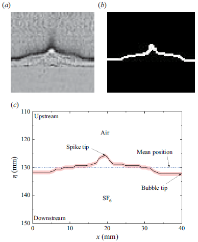
In this study, one-dimensional Fourier analysis is employed to determine the mean interface position, which serves as a reference for distinguishing the bubble and spike structures. For clarity, the Fourier analysis process is summarised in the following steps, with a frame from the V-shaped case at
 $t=103$
 $\unicode {x03BC}$
s as a representative example.
-
(i) Preprocessing. A region spanning one perturbation wavelength, as shown in figure 11(a), is first selected. Using computer-assisted greyscale recognition and thresholding techniques, the original experimental image is converted into a binary image as presented in figure 11(b). The interface contour is identified from the binary image and is subsequently converted into physical coordinates, as illustrated in figure 11(c), thereby yielding a single-valued interface function
 $\eta = \eta (x)$
required for subsequent Fourier analysis, where
$x$
represents the spanwise coordinate.
-
(ii) Fourier analysis. The interface function
$\eta = \eta (x)$
is decomposed using Fourier series expansion as(B1)where
\begin{align} \eta (x)=c_0+a\sum _{n=1}^{\infty }c_n\cos(nkx), \end{align}
$c_0$
denotes the zeroth-order mode, representing the mean interface position, and the coefficients
$c_n$
correspond to the normalised amplitudes of higher-order perturbation modes. The coefficient
$c_0$
is extracted for each image frame, from which the trajectory of the mean interface position and interface velocity jump
$\Delta u$
are obtained. For the interface contour shown in figure 11(c), the Fourier analysis yields
$c_0$
with value 130.07 mm.
-
(iii) Bubble and spike amplitude determination. The bubble amplitude
$a_b$
and spike amplitude
$a_s$
are determined by subtracting the mean interface position
$c_0$
from the streamwise coordinates of the bubble and spike tips, respectively. -
(iv) Overall amplitude determination. Based on the obtained values of
$a_b$
and
$a_s$
, the overall interface amplitude can be determined as
$a = (|a_b|+|a_s|)/2$
.


Image preprocessing procedures for Fourier analysis, illustrated with an example frame from the V-shaped case at
 $t=103$
 $\unicode {x03BC}$
s: (a) original experimental image spanning one perturbation wavelength; (b) binarised image; (c) interface contour in physical coordinates.

It is noteworthy that the mean interface position obtained from Fourier analysis, corresponding to the unperturbed component with
 $k = 0$
, is mathematically equivalent to the position defined by the equal bubble–spike volume criterion, i.e. the location where the area of the downstream bubble region equals that of the upstream spike region. The detailed derivation is presented below.
We define the interface profile at a given time as a function
 $\eta = \eta (x)$
over a single period
 $x\in [0,\lambda ]$
. The Fourier series of the interface function is given by (B1). The zeroth-order mode, denoted by
 $c_0$
, naturally serves as a reference position because it defines the ‘centreline’ of the interface irrespective of higher-order modulations, and this definition has been widely adopted in previous studies (Zhou et al. Reference Zhou2021; Zhou Reference Zhou2024).
The position that separates the interface into equal bubble and spike volumes,
 $y_0$
, is determined by the condition
 \begin{align} \int _{0}^{\lambda }[\eta (x)-y_0]\,\mathrm{d}x=0. \end{align}
Rearranging (B2) yields
 \begin{align} y_0=\frac {1}{\lambda }\int _{0}^{\lambda }\eta (x)\,\mathrm{d}x. \end{align}
By substituting (B1) into (B3) and integrating over an integer multiple of the period, the integral of
 $\cos(nkx)$
vanishes, resulting in
 \begin{align} y_0=\frac {1}{\lambda }\int _{0}^{\lambda }c_0\,\mathrm{d}x=c_0. \end{align}
Therefore, the mean interface positions obtained from these two approaches are identical, and the choice between them does not affect the measured
 $a_b$
and
 $a_s$
.