1 Introduction
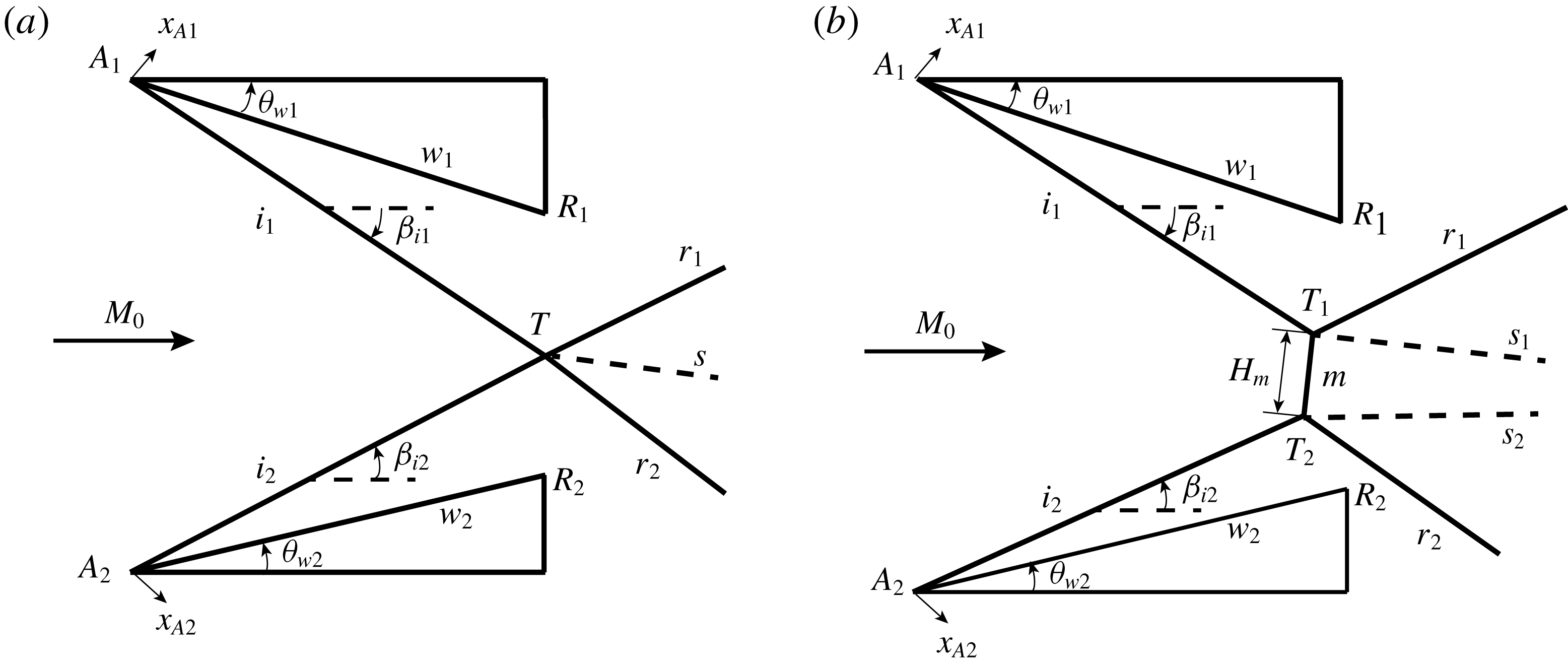
Asymmetrical reflection occurs when steady supersonic flow (with Mach number
 $M_{0}>1$
) encounters two wedges of different geometries. As shown in figure 1, these differences mean that the angle (
 $\unicode[STIX]{x1D703}_{w1}$
), wedge tip abscise (
 $x_{A1}$
) and wedge lower surface length (
 $w_{1}$
) of the upper wedge are generally different from the angle (
 $\unicode[STIX]{x1D703}_{w2}$
), wedge tip abscise (
 $x_{A2}$
) and wedge upper surface length (
 $w_{2}$
) of the lower wedge. Symmetrical shock reflection corresponds to the particular case with
 $\unicode[STIX]{x1D703}_{w1}=\unicode[STIX]{x1D703}_{w2}=\unicode[STIX]{x1D703}_{w}$
,
 $x_{A1}=x_{A2}$
and
 $w_{1}=w_{2}$
. The types of shock reflection, transition between various types and the shape and size of important structures are of primary importance in shock reflection studies and applications.
Depending on
 $M_{0}$
and the wedge angles, there are two types of shock reflection: regular reflection (RR) and Mach reflection (MR), as displayed in figure 1. The criteria and the processes for transition from RR to MR and vice versa have been well established for symmetrical reflection (von Neumann Reference von Neumann1943; Henderson & Lozzi Reference Henderson and Lozzi1975; Hornung, Oertel & Sandeman Reference Hornung, Oertel and Sandeman1979; Ben-Dor et al.
Reference Ben-Dor, Ivanov, Vasilev and Elperin2002; Hornung Reference Hornung2014) and asymmetrical reflection (Chpoun & Lengrand Reference Chpoun and Lengrand1997; Li, Chpoun & Ben-Dor Reference Li, Chpoun and Ben-Dor1999; Ivanov et al.
Reference Ivanov, Ben-Dor, Elperin, Kudryavtsev and Khotyanovsky2002). These two issues are not the concern of the present study. We are particularly interested in the shape and size of the main flow structures such as shock waves and sliplines.
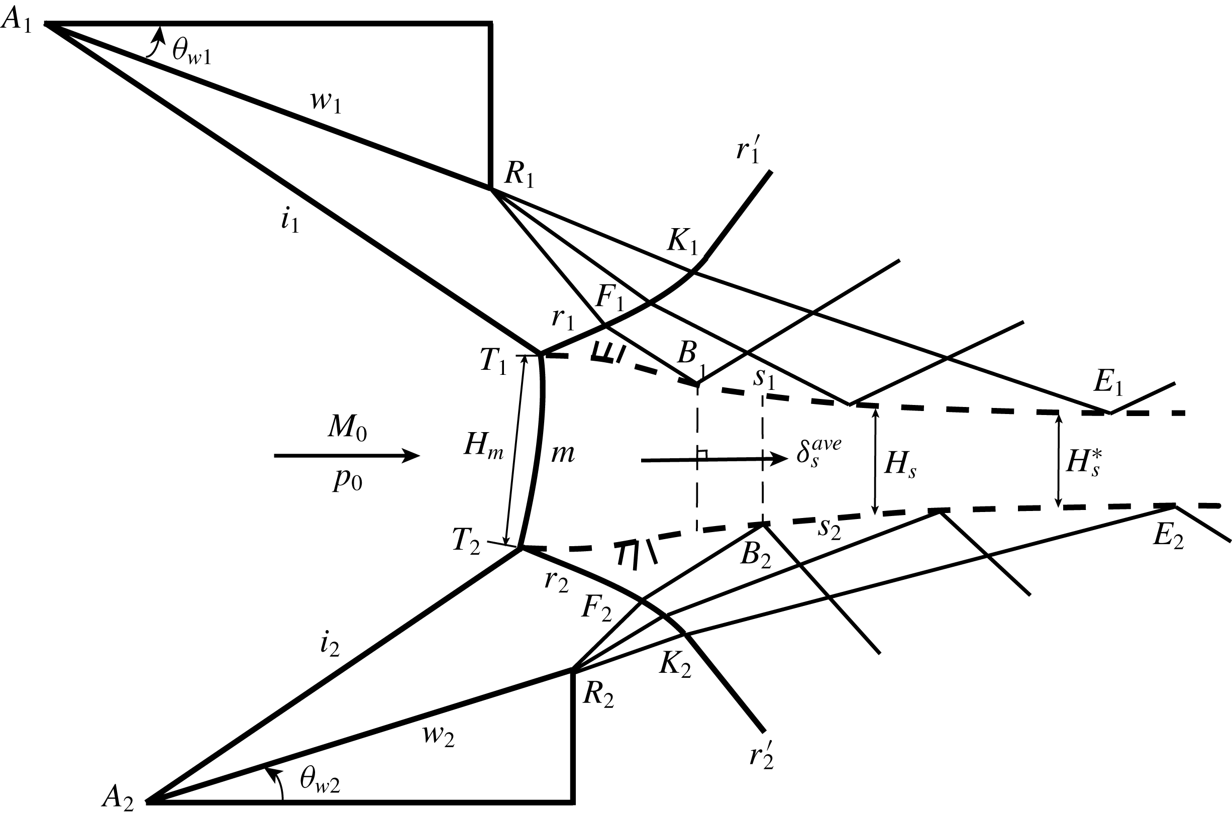
Schematic illustration of asymmetrical shock reflection: (a) regular reflection, (b) Mach reflection. In both cases,
 $i,r$
,
 $s$
and
 $T$
refer to incident shock wave, reflected shock wave, slipline and triple point, respectively. The distance between the two triple points
 $T_{1}$
and
 $T_{2}$
defines the Mach stem height
 $H_{m}$
.

The shape of the various waves in Mach reflection has been studied only for symmetrical shock reflection. For pseudo-steady Mach reflection, Dewey & McMillin (Reference Dewey and McMillin1985a ,Reference Dewey and McMillin b ) made a detailed study of the shapes of the incident, reflected and Mach stem shocks and showed that the reflected shock wave is circular and the Mach stem was described well by a circular arc. Their experimental results were verified by Olim & Dewey (Reference Olim and Dewey1992) and Dewey & Barss (Reference Dewey and Barss1996). The shape of the Mach stem has also been studied analytically by Li, Ben-Dor & Han (Reference Li, Ben-Dor and Han1994) for pseudo-steady reflections, and by Li & Ben-Dor (Reference Li and Ben-Dor1997) for steady flows from a geometrical point of view. For steady Mach reflection, Tan, Ren & Wu (Reference Tan, Ren and Wu2006) derived a very simple algebraic expression for the shape of the Mach stem which can be approximated by a circular arc centred on the reflecting surface. The reflected shock wave is curved upward by the wedge rear corner expansion fan and the shape was calculated analytically by Bai & Wu (Reference Bai and Wu2017). Gao & Wu (Reference Gao and Wu2010) found that the slipline is curved even before touched by the leading characteristics of this expansion fan, due to secondary expansion waves generated over the slipline to balance the pressure decrease along the quasi-one-dimensional flow duct below the slipline. The leading characteristics of the expansion fan induces a slope discontinuity of the slipline, causing a slipline turning shock wave (Bai & Wu Reference Bai and Wu2017).
The Mach stem height (
 $H_{m}$
) has been studied for both symmetrical and asymmetrical cases. Hornung & Robinson (Reference Hornung and Robinson1982) performed experimental measurements of the Mach stem height of symmetrical Mach reflection. They argued that the relative Mach stem height (
 $H_{m}/w$
) is a function of
 $M_{0}$
,
 $\unicode[STIX]{x1D703}_{w}$
,
 $g/w$
and
 $\unicode[STIX]{x1D6FE}$
. Here
 $g$
is the height of the wedge rear corner with respect to the reflecting surface, and
 $\unicode[STIX]{x1D6FE}$
is the ratio of the specific heats of the gas. Hornung & Robinson (Reference Hornung and Robinson1982) provided experimental data for
 $H_{m}/w$
as a function of Mach number and shock angle, which were then used by subsequent authors to test their models. Simplified theoretical models for the Mach stem height of symmetrical Mach reflection have been proposed by Azevedo & Liu (Reference Azevedo and Liu1993), Li & Ben-Dor (Reference Li and Ben-Dor1997), Mouton & Hornung (Reference Mouton and Hornung2007), Gao & Wu (Reference Gao and Wu2010) and Bai & Wu (Reference Bai and Wu2017). In all these models, a quasi-one-dimensional potential flow model is used to treat the flow below the slipline.
The wave interaction with the slipline have been treated with various degrees of complexity in these studies. Bai & Wu (Reference Bai and Wu2017) incorporated analytical models to treat the curved slipline and curved reflected shock waves accounting for the most detailed physics that can be treated analytically. The mechanism by which the size of the Mach stem is determined has been a concern since Courant & Friedrichs (Reference Courant and Friedrichs1948) and Li & Ben-Dor (Reference Li and Ben-Dor1997) pointed out that the expansion fan due to the wedge determines the size and location of the Mach stem by creating the sonic throat and carrying information on the upper geometrical conditions through the subsonic pocket to the Mach stem. For this mechanism to be explicitly used by the model, Bai & Wu (Reference Bai and Wu2017) proposed the sonic throat compatibility condition. In this condition, sonic point below the slipline (determined by the quasi-one-dimensional flow model) must occur at the point with vanishing slope of the slipline (determined by the slipline/Mach wave interaction model).
Mach stem height (or length) for asymmetrical flow has also been studied, but with little attention. This height is defined as the distance between the two triple points (
 $T_{1}$
and
 $T_{2}$
in figure 1
b). Hornung & Mouton (Reference Hornung and Mouton2008), Mouton (Reference Mouton2008) and Mouton & Hornung (Reference Mouton and Hornung2008) simply defined an equivalence shock angle and applied a symmetrical model to estimate this Mach stem height. This simplification cannot account for the effect of relative horizontal position of the wedges. Roy & Rajesh (Reference Roy and Rajesh2017) treated the asymmetrical Mach reflection configuration as the combination of upper and lower domains of symmetrical Mach reflection, in which the symmetry plane served as a common horizontal axis. Tao et al. (Reference Tao, Liu, Fan, Xiong, Yu and Sun2017) made a direct extension of the symmetrical model of Gao & Wu (Reference Gao and Wu2010) to estimate the Mach stem height for asymmetrical Mach reflection. None of these studies considered the shapes of various flow structures.
In this paper, we use both numerical simulation by computational fluid dynamics (CFD) and simplified theoretical analysis to study the influence of various geometrical conditions (difference of wedge angles, horizontal shift of the leading edges of the two wedges, difference of wedge lengths) on the Mach stem height and shape, shape of reflected shock waves and sliplines, nature of sonic throat and horizontal shift of the locations of the two triple points.
The CFD method and the theoretical model are presented in § 2. The theoretical model is updated from the symmetrical model of Bai & Wu (Reference Bai and Wu2017), accounting for new features of asymmetrical reflection as revealed by CFD results. Comparative study of the results are presented in § 3, including the comparison between the theoretical results and other experimental/numerical results. Conclusions will be summarized in § 4. Appendix A includes some details of the theoretical model.
2 CFD method and analytical model of asymmetrical shock wave reflection
The CFD method used in this paper is presented in § 2.1, where a grid refinement study is also performed. A CFD result is demonstrated to reveal the new features of asymmetrical Mach reflection, compared to symmetrical one. The models pertinent to these new features are presented in § 2.2. The overall model for asymmetrical configuration is updated from the symmetrical model of Bai & Wu (Reference Bai and Wu2017) by accounting for these new features. The overall model and the major assumptions are summarized in § 2.3, with mathematical details moved to appendix A. The overall model is attempted to give the shape, location and size of the Mach stem, sliplines and reflected shock waves for a given condition, and is capable of showing how the asymmetrical Mach reflection is affected by the asymmetry of the wedges.
2.1 CFD method and some numerical results
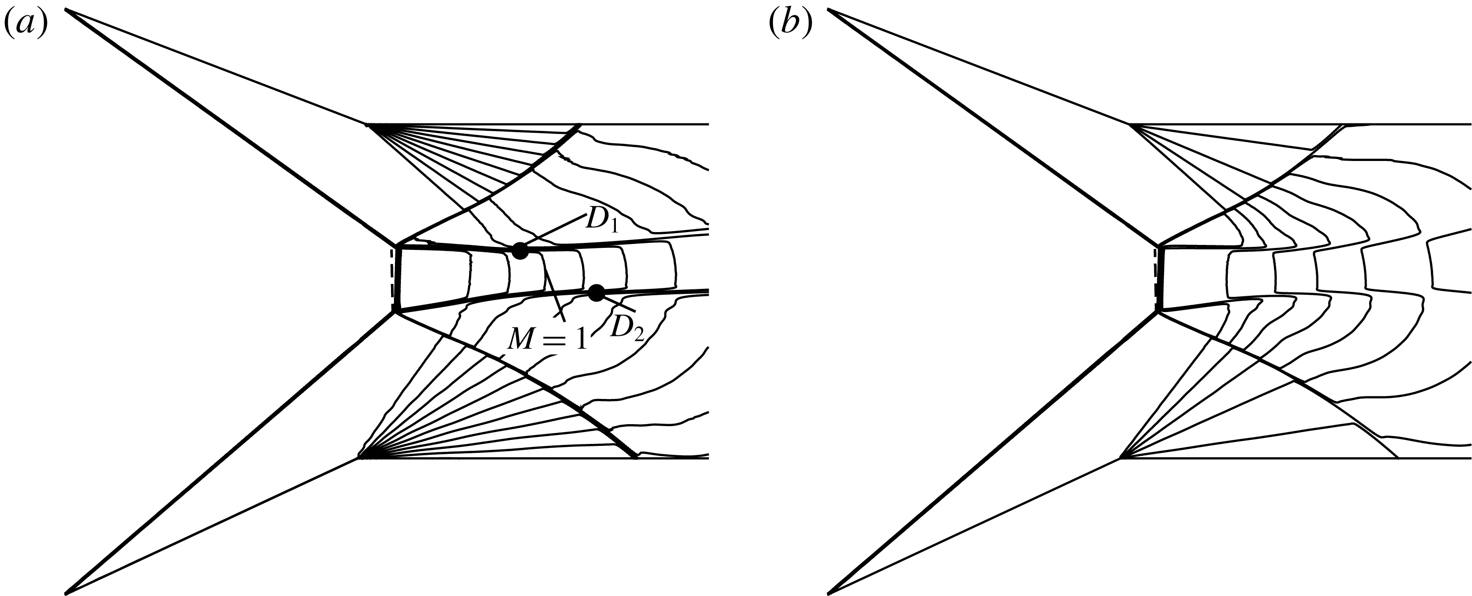
For CFD, the compressible Euler equations in gas dynamics are solved using the second-order Roe scheme (Roe Reference Roe1986), which exists in the commercial code Fluent. The Mach number contours and density contours for asymmetrical reflection with
 $M_{0}=3.5$
,
 $\unicode[STIX]{x1D703}_{w1}=21^{\circ }$
,
 $\unicode[STIX]{x1D703}_{w2}=25^{\circ }$
,
 $w_{1}/H_{A}=w_{2}/H_{A}=0.55$
,
 $d/H_{A}=0$
are displayed in figure 2, in which the dashed line is a vertical line (showing the Mach stem is not vertical) and the points
 $D_{1}$
and
 $D_{2}$
are locations of the sliplines
 $s_{1}$
and
 $s_{2}$
with vanishing slope. These results have been obtained using a structured grid with
 $1000\times 600$
points. It is seen that, for this asymmetrical flow case (
 $\unicode[STIX]{x1D703}_{w1}=21^{\circ }$
,
 $\unicode[STIX]{x1D703}_{w2}=25^{\circ }$
), the horizontal positions of the two triple points are different, and the slopes of the two sliplines do not vanish at the sonic throat (with
 $M=1$
). Moreover, the quasi-one-dimensional flow duct between the sliplines does not follow the horizontal direction. These are new features pertinent to asymmetrical Mach reflection.
Mach number contours (a) and density contours (b) showing the structure of flow field for asymmetrical reflection with
 $M_{0}=3.5$
,
 $\unicode[STIX]{x1D703}_{w1}=21^{\circ }$
,
 $\unicode[STIX]{x1D703}_{w2}=25^{\circ }$
,
 $w_{1}/H_{A}=w_{2}/H_{A}=0.55$
,
 $d/H_{A}=0$
.

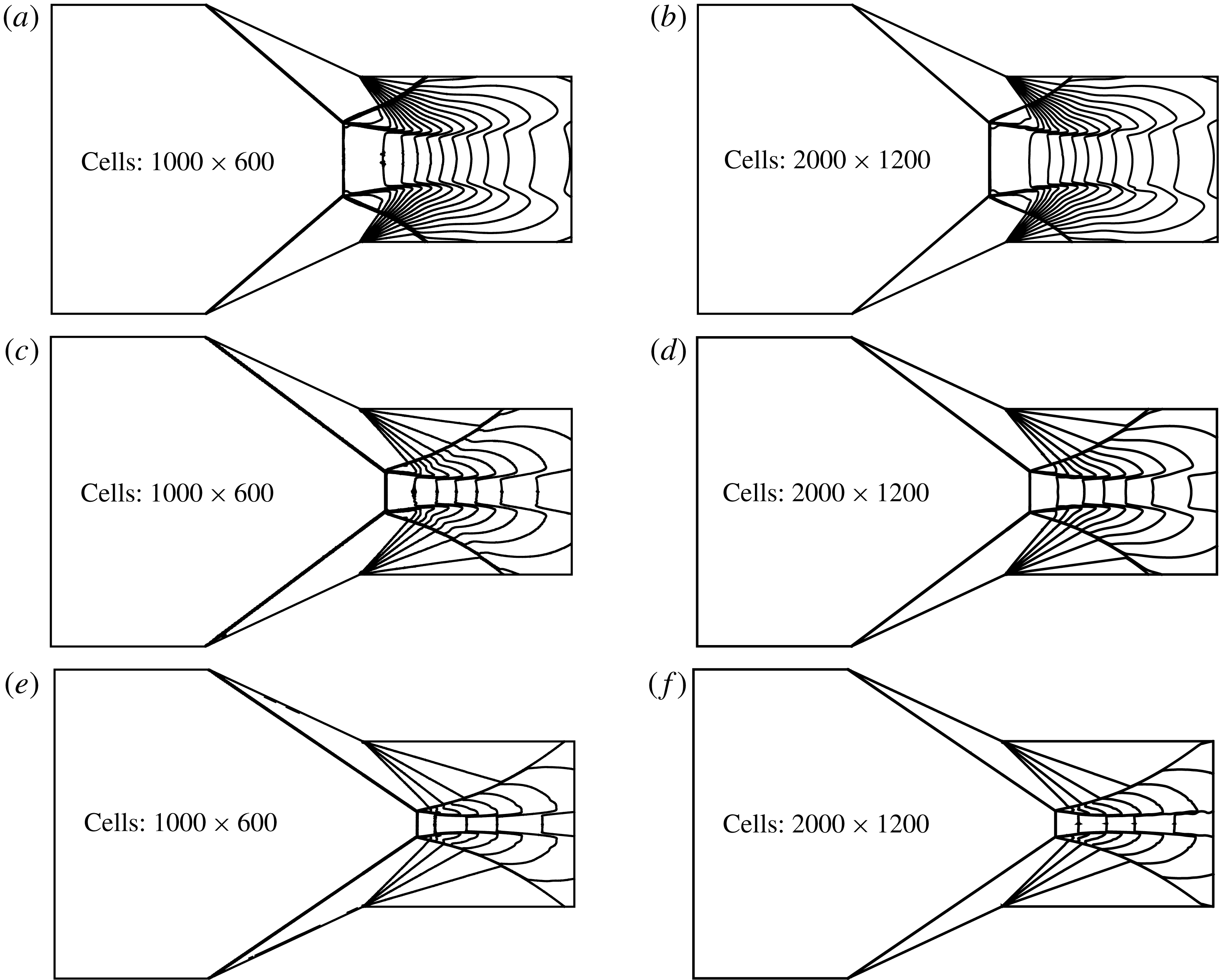
To see if the grid used is fine enough, a grid with
 $1000\times 600$
points and a grid with
 $2000\times 1200$
points are used to compute the symmetrical flow with
 $\unicode[STIX]{x1D703}_{w1}=\unicode[STIX]{x1D703}_{w2}=25^{\circ }$
,
 $w_{1}/H_{A}=w_{2}/H_{A}=0.55$
,
 $d/H_{A}=0$
for
 $M_{0}=3.5$
, 4.5 and 6. The asymmetrical cases are equally mesh converged as the symmetrical cases because the meshes are very similar in the symmetrical and asymmetrical cases and their convergence is nearly identical, which is not shown here. The density contours are displayed in figure 3. It is seen that the overall configurations for both grids are very similar to each other.
We are unable to measure any difference of the heights of Mach stem and sonic throat for both grids, they are
 $H_{m}/H_{A}=$
 $0.246$
, 0.135, 0.085 and
 $H_{s}/H_{A}=0.161$
, 0.086, 0.052 for
 $M_{0}=3.5$
, 4.5 and 6. Since there is no essential difference in the results between the two grids, the grid with
 $1000\times 600$
points is used throughout the rest of this paper. In addition, the numerical solutions are shown later in the paper to have good agreement with the theory, which agrees well with experimental and CFD results of previous studies, and also verifies the validation of the numerical simulation method and mesh.
As stated in Ivanov et al. (Reference Ivanov, Ben-Dor, Elperin, Kudryavtsev and Khotyanovsky2002), the computed flow field was considered as converged to a steady state when the positions of all the shock waves remained unchanged during several non-dimensional time units, which was defined as
 $\unicode[STIX]{x1D70F}=w/a_{0}$
, where
 $w$
is the length of either wedge and
 $a_{0}$
is the free-stream speed of sound. We have therefore run the computation for a sufficiently long time so that the steady state is reached. If the steady state were not reached, then the sliplines have oscillations, which may be interpreted as instabilities. When steady state is reached, no oscillation is observed.
Density contours with two different grids for different Mach numbers (a,b
 $M_{0}=3.5$
, c,d
 $M_{0}=4.5$
, e,f
 $M_{0}=6$
). The other conditions are the same and are given by
 $\unicode[STIX]{x1D703}_{w1}=\unicode[STIX]{x1D703}_{w2}=25^{\circ }$
,
 $w_{1}/H_{A}=w_{2}/H_{A}=0.55$
,
 $d/H_{A}=0$
.

2.2 New features and analytical methods pertinent to asymmetrical reflection
In this subsection, the new features and overall configuration of asymmetrical Mach reflection are first summarized, then analytical models are given for each new feature.
2.2.1 Summary of new features and the overall configuration of asymmetrical Mach reflection
From the CFD result shown above, it is seen that the asymmetrical flow case displays the following new characteristics:
(i) The two triple points in the asymmetrical case may have a horizontal shift so that the shape of the Mach stem must be treated differently compared to the symmetrical case (see § 2.2.2 for this treatment).
(ii) The quasi-one-dimensional flow duct between the sliplines does not follow the horizontal direction, it has an averaged flow direction that varies in the downstream direction and should be determined as an unknown property (see § 2.2.3 for the quasi-one-dimensional model and a pressure balance equation associated with this model).
(iii) The most important new feature is that the sonic throat does not occur at points where the slopes of sliplines vanish, this means that the sonic throat compatibility condition of symmetrical reflection should be revised (see § 2.2.4 for details of this new condition).
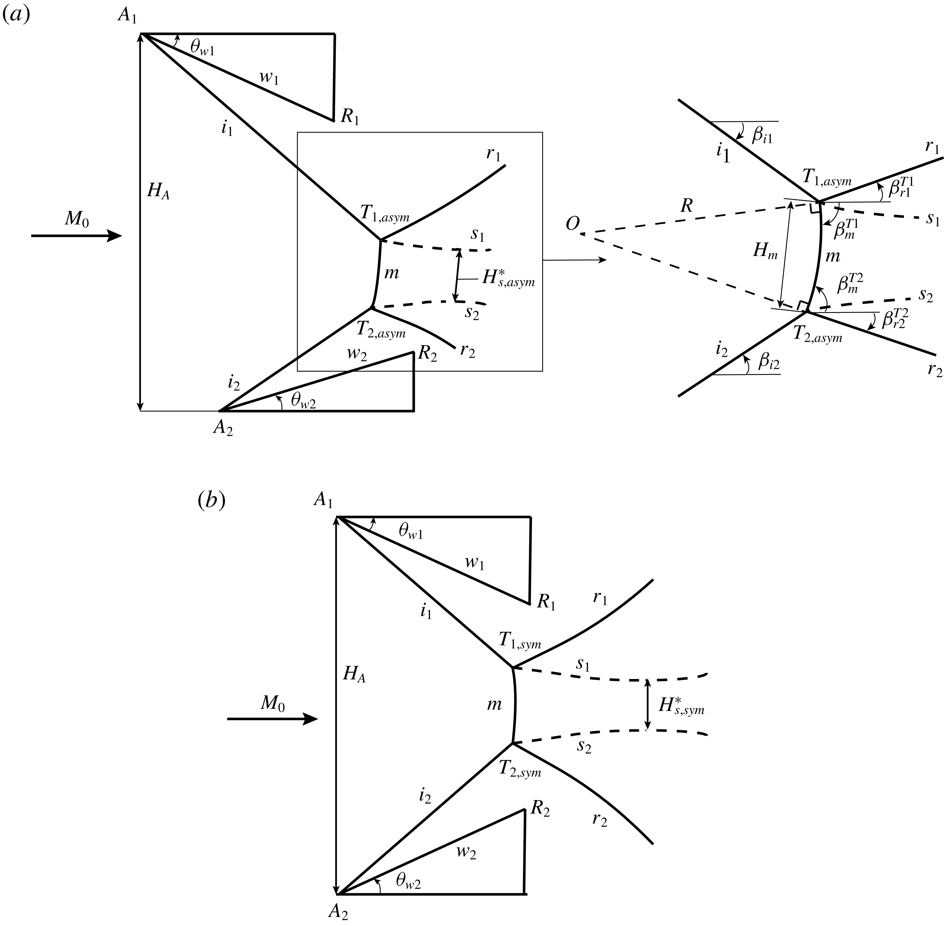
Based on the numerical solutions as shown in figure 2, the main structures for asymmetrical Mach reflections are depicted in figure 4(a). For comparison, figure 4(b) displays the structures for a symmetrical flow case. In these pictures,
 $T_{1,sym}$
and
 $T_{2,sym}$
are triple points of symmetrical Mach reflection,
 $T_{1,asym}$
and
 $T_{2,asym}$
are the triple points of asymmetrical Mach reflection. The expansion fans at the trailing edge of wedges are not drawn here.
Schematic illustration of flow structures for asymmetrical (a) and symmetrical (b) Mach reflection.

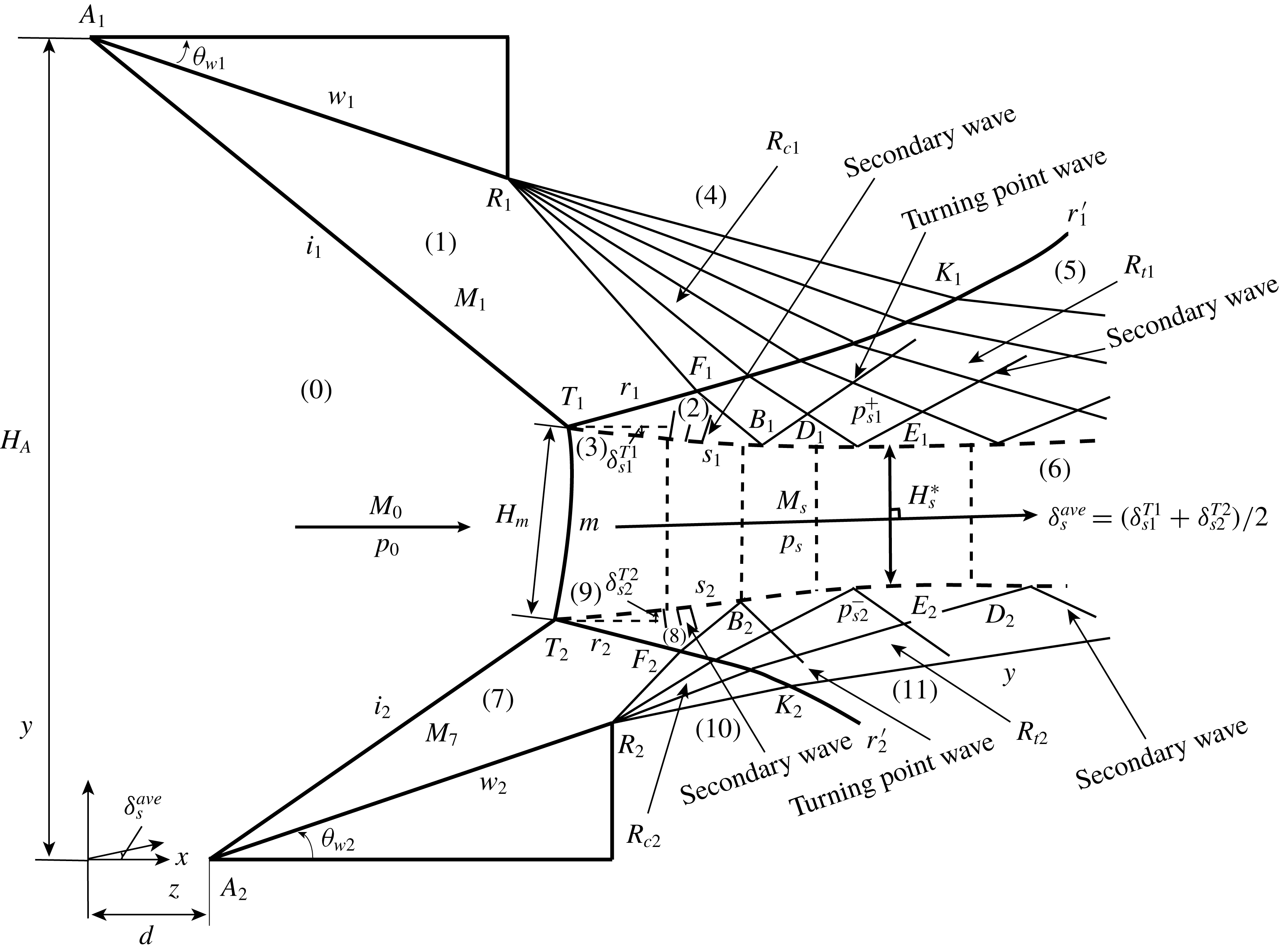
The overall model will be built following figure 5. The flow is composed of two incident shock waves
 $(i_{1})$
,
 $(i_{2})$
, two reflected shock waves
 $(r_{1})$
,
 $(r_{2})$
, one Mach stem
 $(m)$
and two sliplines
 $(s_{1})$
,
 $(s_{2})$
. These discontinuities are connected by two triple points
 $T_{1}$
,
 $T_{2}$
. The waves
 $(R_{c1})$
,
 $(R_{c2})$
are Mach waves inside expansion fans from the wedge corners
 $R_{1}$
,
 $R_{2}$
and
 $(R_{t1})$
,
 $(R_{t2})$
are transmitted Mach waves coming from the interaction of the expansion fans with the reflected shock waves. The leading characteristics of the transmitted expansion wave
 $R_{t1}$
and
 $R_{t2}$
intersects the slipline
 $s_{1}$
and
 $s_{2}$
at
 $B_{1}$
and
 $B_{2}$
(called turning points by Bai & Wu Reference Bai and Wu2017).
The flow between the two sliplines is considered as quasi-one-dimensional and is composed of a subsonic pocket (before the sonic throat
 $H_{s}^{\ast }$
) and a supersonic pocket (behind
 $H_{s}^{\ast }$
). The direction of the quasi-one-dimensional flow is assumed to follow the axis
 $oz$
, with
 $\measuredangle zox=\unicode[STIX]{x1D6FF}_{s}^{ave}$
(anti-clockwise is positive), which is defined in (2.5).
The deflection angles of the slipline
 $s_{1}$
at point
 $D_{1}$
and
 $s_{2}$
at point
 $D_{2}$
satisfy
 $\unicode[STIX]{x1D6FF}_{s}^{D1}=\unicode[STIX]{x1D6FF}_{s}^{D2}=0$
. The line
 $E_{1}E_{2}$
is the sonic throat. The coordinate system is defined such that the
 $x$
-axis is along the incoming flow direction and passes through the point
 $A_{2}$
, and the
 $y$
-axis passes through the point
 $A_{1}$
. In this coordinate system
 $A_{1}$
is at
 $(0,H_{A})$
and
 $A_{2}$
is at
 $(d,0)$
. The height
 $H_{A}$
and horizontal shift
 $d$
of the two wedge leading edges are given properties. For such a coordinate system, the positions of the trailing edges
 $R_{1}$
and
 $R_{2}$
are given by
 $$\begin{eqnarray}\left.\begin{array}{@{}c@{}}x_{R1}=w_{1}\cos \unicode[STIX]{x1D703}_{w1},\quad y_{R_{1}}=H_{A}-w_{1}\sin \unicode[STIX]{x1D703}_{w1},\\ x_{R2}=d+w_{2}\cos \unicode[STIX]{x1D703}_{w2},\quad y_{R2}=w_{2}\sin \unicode[STIX]{x1D703}_{w2},\end{array}\right\}\end{eqnarray}$$
where
 $w_{1},w_{2},\unicode[STIX]{x1D703}_{w1}$
and
 $\unicode[STIX]{x1D703}_{w2}$
are given properties of the two wedges.
Schematic of asymmetrical Mach reflection.

2.2.2 Relations for triple point positions and shape of the Mach stem
As for symmetrical Mach reflection, a model is needed for the shape of the Mach stem. Here this shape is related to two triple points which may have a horizontal shift. The positions of the two triple points are related by the shock angles of incident shock waves and by the shape of the Mach stem.
Among various possibilities, we find that assuming the Mach stem to be a circular arc leads to a minimal number of unknowns that may be related by an equal number of physical relations, provided the height of the Mach stem is determined by a more global algorithm as described in § 2.3. The rationality of circular arc assumption for Mach stem has been proven for symmetrical reflection (Dewey & McMillin Reference Dewey and McMillin1985a ,Reference Dewey and McMillin b ; Olim & Dewey Reference Olim and Dewey1992; Li et al. Reference Li, Ben-Dor and Han1994; Dewey & Barss Reference Dewey and Barss1996; Li & Ben-Dor Reference Li and Ben-Dor1997; Tan et al. Reference Tan, Ren and Wu2006). Here we adopt this assumption just for purpose of having a simple model with a minimal number of unknowns.
As displayed in figure 4(a), the Mach stem is now assumed to lie on a circle of radius
 $R$
and centred at
 $O(x_{O},y_{O})$
.
The fact that the triple points
 $T_{1}$
and
 $T_{2}$
lie on the Mach stem (assumed to be circular) and incident shock wave
 $(i_{1})$
and
 $(i_{2})$
means that the following geometrical relations hold
 $$\begin{eqnarray}\left.\begin{array}{@{}c@{}}y_{T1}-y_{A1}=(x_{T1}-x_{A1})\tan \unicode[STIX]{x1D6FD}_{i1},\\ y_{T2}-y_{A2}=(x_{T2}-x_{A2})\tan \unicode[STIX]{x1D6FD}_{i2},\\ (x_{T1}-x_{O})^{2}+(y_{T1}-y_{O})^{2}=R^{2},\\ (x_{T2}-x_{O})^{2}+(y_{T2}-y_{O})^{2}=R^{2}.\end{array}\right\}\end{eqnarray}$$
The four relations in (2.2) involve seven unknowns
 $x_{O}$
,
 $y_{O}$
,
 $R$
,
 $x_{T1}$
,
 $y_{T1}$
,
 $x_{T2}$
,
 $y_{T2}$
. A further relation is obtained by assuming the Mach stem height
 $H_{m}$
is the distance between the two triple points
 $$\begin{eqnarray}(x_{T_{2}}-x_{T_{1}})^{2}+(y_{T_{2}}-y_{T_{1}})^{2}=H_{m}^{2}.\end{eqnarray}$$
The circular shape relation
 $(x-x_{O})^{2}+(y-y_{O})^{2}=R^{2}$
of the Mach stem can be used to obtain the slopes of the Mach stem at the triple points, and these slopes are equal to the tangent of shock angles
 $\unicode[STIX]{x1D6FD}_{m}^{T1}$
and
 $\unicode[STIX]{x1D6FD}_{m}^{T2}$
. This gives two further geometrical relations
 $$\begin{eqnarray}\left.\begin{array}{@{}c@{}}k_{OT1}={\displaystyle \frac{y_{T1}-y_{O}}{x_{T1}-x_{O}}}=-{\displaystyle \frac{1}{\tan (\unicode[STIX]{x1D6FD}_{m}^{T1})}},\\ k_{OT2}={\displaystyle \frac{y_{T2}-y_{O}}{x_{T2}-x_{O}}}=-{\displaystyle \frac{1}{\tan (\unicode[STIX]{x1D6FD}_{m}^{T2})}}.\end{array}\right\}\end{eqnarray}$$
With
 $\unicode[STIX]{x1D6FD}_{m}^{T1}$
and
 $\unicode[STIX]{x1D6FD}_{m}^{T2}$
determined by the three-shock theory of von Neumann (Reference von Neumann1943) and with
 $H_{m}$
prescribed or determined by the algorithm in § 2.3, the relations (2.2)–(2.4) can be used to uniquely determine
 $x_{O}$
,
 $y_{O}$
,
 $R$
,
 $x_{T1}$
,
 $y_{T1}$
,
 $x_{T2}$
,
 $y_{T2}$
.
2.2.3 The quasi-one-dimensional flow model and pressure balance conditions
In symmetrical reflection, the flow in the duct between the sliplines has been treated using the quasi-one-dimensional isentropic flow model (e.g. Azevedo & Liu Reference Azevedo and Liu1993; Li & Ben-Dor Reference Li and Ben-Dor1997; Gao & Wu Reference Gao and Wu2010; Bai & Wu Reference Bai and Wu2017). This approach was followed by Tao et al. (Reference Tao, Liu, Fan, Xiong, Yu and Sun2017) for asymmetrical reflection.
In contrast to the symmetrical flow case where the flow is horizontal, here the averaged flow direction may be non-horizontal. The inlet of the duct is non-vertical due to the asymmetry of the two triple points and the two sliplines may not evolve in such a way that a preferable local flow direction can be properly defined. Various ways can be invented to build a quasi-one-dimensional flow model. Here we prefer to use the simplest one, the suitability of which will be justified by its good comparison with numerical results in § 3.
The inlet of the flow duct is determined by the two triple points, the positions of which are given by the relations in § 2.2.2. As shown in figure 5, the direction of the inlet is simply evaluated using
 $$\begin{eqnarray}\unicode[STIX]{x1D6FF}_{s}^{ave}={\textstyle \frac{1}{2}}(\unicode[STIX]{x1D6FF}_{s1}^{T1}+\unicode[STIX]{x1D6FF}_{s2}^{T2}),\end{eqnarray}$$
where
 $\unicode[STIX]{x1D6FF}_{s1}^{T1}$
and
 $\unicode[STIX]{x1D6FF}_{s2}^{T2}$
are the deflection angles of sliplines
 $s_{1}$
and
 $s_{2}$
near the triple points
 $T_{1}$
and
 $T_{2}$
, which are calculated by the three-shock theory. The normal direction of the cross-section of the quasi-one-dimensional duct is assumed to follow this initial direction (with
 $z$
measuring the distance) in all positions along the downstream direction. The averaged flow properties at any location
 $z$
are defined along a segment perpendicular to the direction
 $\unicode[STIX]{x1D6FF}_{s}^{ave}$
. The averaged velocity is assumed to be along the direction
 $z$
. In fact, in the following model to determine the Mach reflection configuration, this velocity does not need to appear explicitly.
Then we add a half-line
 $oz$
originating from
 $o$
, which satisfies that angle
 $\measuredangle zox$
is equal to
 $\unicode[STIX]{x1D6FF}_{s}^{ave}$
(anti-clockwise is positive).
Cross-section of the duct is the section over which the averaged flow parameters are defined. These averaged parameters include the pressure
 $p_{s}(z)$
and Mach number
 $M_{s}(z)$
. In symmetrical shock wave reflection, the cross-section is in the vertical direction, with its height
 $H_{s}(z)$
given by the vertical position of the slipline. In asymmetrical shock wave reflection, the cross-section is inclined and is assumed to be perpendicular to the direction
 $\unicode[STIX]{x1D6FF}_{s}^{ave}$
. The height (which may be better called the length)
 $H_{s}(z)$
is evaluated as the distance between the two sliplines
 $s_{1}$
and
 $s_{2}$
(the model for which is presented in § 2.3), measured along the direction parallel to this cross-section.
The standard quasi-one-dimensional isentropic flow model is then directly used in its original form to connect the averaged pressure
 $p_{s}(z)$
and Mach number
 $M_{s}(z)$
to the height of the cross-section
 $H_{s}(z)$
, i.e.
 $$\begin{eqnarray}\left.\begin{array}{@{}c@{}}{\displaystyle \frac{\text{d}p_{s}(z)}{\text{d}z}}=p_{s}{\displaystyle \frac{\unicode[STIX]{x1D6FE}M_{s}^{2}}{1-M_{s}^{2}}}{\displaystyle \frac{1}{H_{s}}}{\displaystyle \frac{\text{d}H_{s}}{\text{d}z}},\\ M_{s}(z)=\sqrt{{\displaystyle \frac{2}{\unicode[STIX]{x1D6FE}-1}}\left(\left(1+{\displaystyle \frac{\unicode[STIX]{x1D6FE}-1}{2}}M_{m}^{2}\right)\left({\displaystyle \frac{p_{s}}{p_{m}}}\right)^{-(\unicode[STIX]{x1D6FE}-1/\unicode[STIX]{x1D6FE})}-1\right)},\end{array}\right\}\end{eqnarray}$$
where
 $M_{m}$
and
 $p_{m}$
are the inlet condition of the quasi-one-dimensional flow model defined in (A 1).
All previous authors simply assume the pressure to be continuous across the slipline (symmetrical case) or sliplines (asymmetrical case). For the symmetrical case, Bai & Wu (Reference Bai and Wu2017) divided the slipline into a free part and an interacting part, divided by the first leading characteristics of the wedge expansion fan and treated differently for the pressure balance.
Here, for the asymmetrical case, we follow Bai & Wu (Reference Bai and Wu2017), with pressure balance imposed on both sides of the free part of each slipline, and with pressure gradient balance imposed on both sides of the interacting part of each slipline.
Specifically, for the free part, the pressure balance is
 $$\begin{eqnarray}p_{s1}^{+}(z)=p_{s}(z)=p_{s2}^{-}(z)\end{eqnarray}$$
in which
 $p_{s1}^{+}(z)$
and
 $p_{s2}^{-}(z)$
are the pressures above the upper slipline
 $s_{1}$
and beneath the lower slipline
 $s_{2}$
. For the interacting part, the pressure gradient balance is
 $$\begin{eqnarray}\frac{\text{d}p_{s1}^{+}(z)}{\text{d}z}=\frac{\text{d}p_{s}(z)}{\text{d}z}=\frac{\text{d}p_{s2}^{-}(z)}{\text{d}z}.\end{eqnarray}$$
2.2.4 The sonic throat compatibility condition
As stated in the Introduction, the Mach stem height is determined by the sonic throat compatibility condition for symmetrical reflection (Bai & Wu Reference Bai and Wu2017). This condition states that, the solution is compatible if the sonic throat condition
 $M_{s}=M_{s}^{\ast }=1$
occurs exactly at
 $x_{s}$
with vanishing slipline slope (
 $\unicode[STIX]{x1D6FF}_{s}(x_{s})=0$
,
 $\unicode[STIX]{x1D6FF}_{s}$
is the deflection angle of the slipline in symmetrical reflection).
For asymmetrical reflection, the slopes of the two sliplines do not vanish at the same position. As shown in figure 5, the points
 $D_{1}$
and
 $D_{2}$
are the locations of sliplines
 $s_{1}$
and
 $s_{2}$
with vanishing slope and they do not have the same location
 $z$
. The sonic throat (
 $E_{1}E_{2}$
) locates between
 $D_{1}$
and
 $D_{2}$
. Thus the sonic throat compatibility condition must be revised for asymmetrical flow.
Within the framework of simplified quasi-one-dimensional flow model, the flow is subsonic in region with
 $\text{d}H_{s}/\text{d}z<0$
and supersonic in region with
 $\text{d}H_{s}/\text{d}z>0$
, and the sonic throat (
 $E_{1}E_{2}$
) locates at
 $\text{d}H_{s}/\text{d}z=0$
.
Geometrically,
 $\text{d}H_{s}/\text{d}z$
is related to the deflection angles
 $\unicode[STIX]{x1D6FF}_{s1}$
and
 $\unicode[STIX]{x1D6FF}_{s2}$
of the two sliplines by
 $\tan \unicode[STIX]{x1D6FF}_{s1}-\tan \unicode[STIX]{x1D6FF}_{s2}=-\text{d}H_{s}/\text{d}x$
. Since
 $\text{d}z=\text{d}x\cos \unicode[STIX]{x1D6FF}_{s}^{ave}$
and
 $\text{d}H_{s}/\text{d}x=(\text{d}H_{s}/\text{d}z)(\text{d}z/\text{d}x)=(\text{d}H_{s}/\text{d}z)\cos \unicode[STIX]{x1D6FF}_{s}^{ave}$
, we have
 $$\begin{eqnarray}\tan \unicode[STIX]{x1D6FF}_{s1}-\tan \unicode[STIX]{x1D6FF}_{s2}=-\frac{\text{d}H_{s}}{\text{d}z}\cos \unicode[STIX]{x1D6FF}_{s}^{ave}.\end{eqnarray}$$
Since
 $\cos \unicode[STIX]{x1D6FF}_{s}^{ave}\neq 0$
, the expression (2.9) means that the sonic throat (
 $E_{1}E_{2}$
) must locate at a position satisfying
 $\unicode[STIX]{x1D6FF}_{s1}(z)-\unicode[STIX]{x1D6FF}_{s2}(z)=0$
. Following the definition (2.5), the direction of the quasi-one-dimensional flow duct is along
 $\unicode[STIX]{x1D6FF}_{s}^{ave}$
, so the sonic line
 $E_{1}E_{2}$
is perpendicular to the direction
 $\unicode[STIX]{x1D6FF}_{s}^{ave}$
.
Thus, the sonic throat compatibility condition in the asymmetrical interaction of shock waves can be thus expressed as
 $$\begin{eqnarray}\left.\begin{array}{@{}c@{}}\unicode[STIX]{x1D6FF}_{s1}^{E1}-\unicode[STIX]{x1D6FF}_{s2}^{E2}=0,\\ M_{s}|_{E1E2}=M_{s}^{\ast }=1,\\ {\displaystyle \frac{y_{E2}-y_{E1}}{x_{E2}-x_{E1}}}=-{\displaystyle \frac{1}{\tan (\unicode[STIX]{x1D6FF}_{s}^{ave})}}.\end{array}\right\}\end{eqnarray}$$
This means that the Mach number in the flow duct is equal to 1 at the location such that the difference of flow deflection angles of the two sliplines vanishes.
2.3 Global model for the asymmetrical Mach reflection configuration
Now we adapt the symmetrical Mach reflection model of Bai & Wu (Reference Bai and Wu2017) to an asymmetrical Mach reflection configuration, accounting for the new features pertinent to asymmetrical reflection, as discussed above. The model thus obtained gives the Mach stem height
 $H_{m}$
, the positions of the two triple points
 $T_{1}$
and
 $T_{2}$
, the shape of the Mach stem, the shape of the sliplines
 $s_{1}$
and
 $s_{2}$
and the shape of the reflected shock waves
 $r_{1}$
and
 $r_{2}$
. The model is based on figure 5 which gives the necessary information (notations, waves, various flow regions) for building the a global algorithm.
The global algorithm contains the following major assumptions, models or steps, occurring in sequential order for iteration when solved computationally. The assumptions and models (for the shape of Mach stem and positions of the triple points, for the quasi-one-dimensional duct flow and pressure balance across splines, and for sonic throat) pertinent to asymmetrical reflection have already been presented in § 2.2.
(i) Incident shock waves and triple points (classical oblique shock wave relations, triple shock theory of von Neumann (Reference von Neumann1943) applied to each triple points). These models give the shock angles and the flow parameters in the uniform flow regions for given
 $M_{0},\unicode[STIX]{x1D703}_{w1}$
and
 $\unicode[STIX]{x1D703}_{w2}$
. With the triple point solution, the averaged values of flow parameters behind the Mach stem (necessary for the quasi-one-dimensional model) can be simply estimated. See § A.1 for more details.
(ii) Initial guess of the Mach stem height
 $H_{m}$
and the triple point positions
 $(x_{T1},y_{T1})$
and
 $(x_{T2},y_{T2})$
. This guess is used to compute the sliplines and reflected shock waves in the following steps and its value will be updated using the sonic compatibility condition. The triple point positions are computed using the relations (2.2)–(2.4) in § 2.2.2. See § A.2 for more details.
(iii) Model for the reflected shock waves. Each reflected shock wave, starting from
 $(x_{T1},y_{T1})$
or
 $(x_{T2},y_{T2})$
as determined above, is split into a free part and an interacting part by the leading characteristics of the expansion fan, similarly as in the symmetrical flow model of Bai & Wu (Reference Bai and Wu2017). The free part is assumed straight, with the shock angle determined by the triple point solution. The interacting part uses the differential shock wave expansion fan interaction model of Bai & Wu (Reference Bai and Wu2017), which gives the local shock angle
 $\unicode[STIX]{x1D6FD}_{r}$
(which then gives the shape
 $y_{r}=y_{r}(x_{r})$
of the shock wave). The model (of the shock shape) for the upper shock wave is exactly the same as in symmetrical case. The solutions downstream of the interacting part will be carried to the sliplines to compute the shape of the sliplines. The model for reflected shock waves is not influenced by the new features as presented in § 2.2. See § A.3 for details.
(iv) Shape and positions of the sliplines. The pressure balance model given in § 2.2.3 is used to obtain the shape of the sliplines. The pressure variation in the region between the sliplines is obtained by using the quasi-one-dimensional flow model as described in § 2.2.3. For the pressure variation on the supersonic flow side of each slipline, the flow physics is different according to whether it is the free part (before
 $B_{1}$
or
 $B_{2}$
in figure 6) or the interacting part (after
 $B_{1}$
or
 $B_{2}$
) of the slipline. For the free part of each slipline, there are secondary expansion waves on the supersonic flow side. The pressure variation due to these secondary expansion waves is related to the shape of the slipline using the differential Prandtl–Meyer relation. For the interacting part, the pressure variation (on each supersonic flow side) is caused by incident Mach waves (which carries the pressure variation just downstream of the reflected shock waves to the sliplines) and secondary shock waves (for which the pressure variation is described by the differential Prandtl–Meyer relation). These incident Mach waves, also called transmitted expansion waves by Bai & Wu (Reference Bai and Wu2017), are Mach waves from the wedge corner expansion fans having transmitted the reflected shock waves. In all these pressure variation models, the pressure variations are then related to the shape of the sliplines. Applying the pressure balance relations (2.7) or (2.8) to each slipline then gives the shape or positions (
 $x_{s},y_{s}$
) of the sliplines. The details are given in § A.4.
The quasi-one-dimensional flow duct is split into three parts: the first part with two free sliplines, the second part with one free slipline and one interacting part and the third part with two interacting sliplines.

(v) Update of the Mach stem height using the sonic throat compatibility condition. In the first step in an iterative process, the Mach stem height
 $H_{m}$
is guessed in order to compute the triple point positions, shape and positions of the reflected shock waves and sliplines. This height should be updated until the sonic throat compatibility condition (2.10) (§ 2.2.4) is met. An iteration method, similar to that of Bai & Wu (Reference Bai and Wu2017), is provided in § A.5 to accomplish this update.
The Mach stem height thus determined should vary according to
 $$\begin{eqnarray}\frac{H_{m}}{H_{A}}=f\left(\unicode[STIX]{x1D6FE},M_{0},\unicode[STIX]{x1D703}_{w1},\unicode[STIX]{x1D703}_{w2},\frac{d}{H_{A}},\frac{w_{1}}{H_{A}},\frac{w_{2}}{H_{A}}\right)\end{eqnarray}$$
which for symmetrical reflection reduces to the functional form given by Hornung & Robinson (Reference Hornung and Robinson1982).
3 Analysis of flow structures of asymmetrical Mach reflection
The asymmetrical Mach reflection model and CFD method presented in § 2 are used here to study the influence of asymmetry of the two wedges (wedge angles
 $\unicode[STIX]{x1D703}_{w1}$
and
 $\unicode[STIX]{x1D703}_{w2}$
, wedge lengths
 $w_{1}$
and
 $w_{2}$
, horizontal shift
 $d=x_{A2}-x_{A1}$
of the wedge leading edges) on the flow structures, including Mach stem height, shape of various shock waves and sliplines. The accuracy of the theory is checked through comparison with CFD results. Section 3.1 details a comparison of the overall flow structure predicted by both theory and CFD and a check of the suitability of the sonic throat compatibility condition. Section 3.2 details the study of the influence of asymmetry on the size and shape of the Mach stem. A comparison between theory and CFD results is also performed in order to assess the accuracy of the model. Section 3.3 is concerned with the effect of horizontal shift of the wedges.
3.1 Overall flow structures and check of the sonic throat compatibility condition
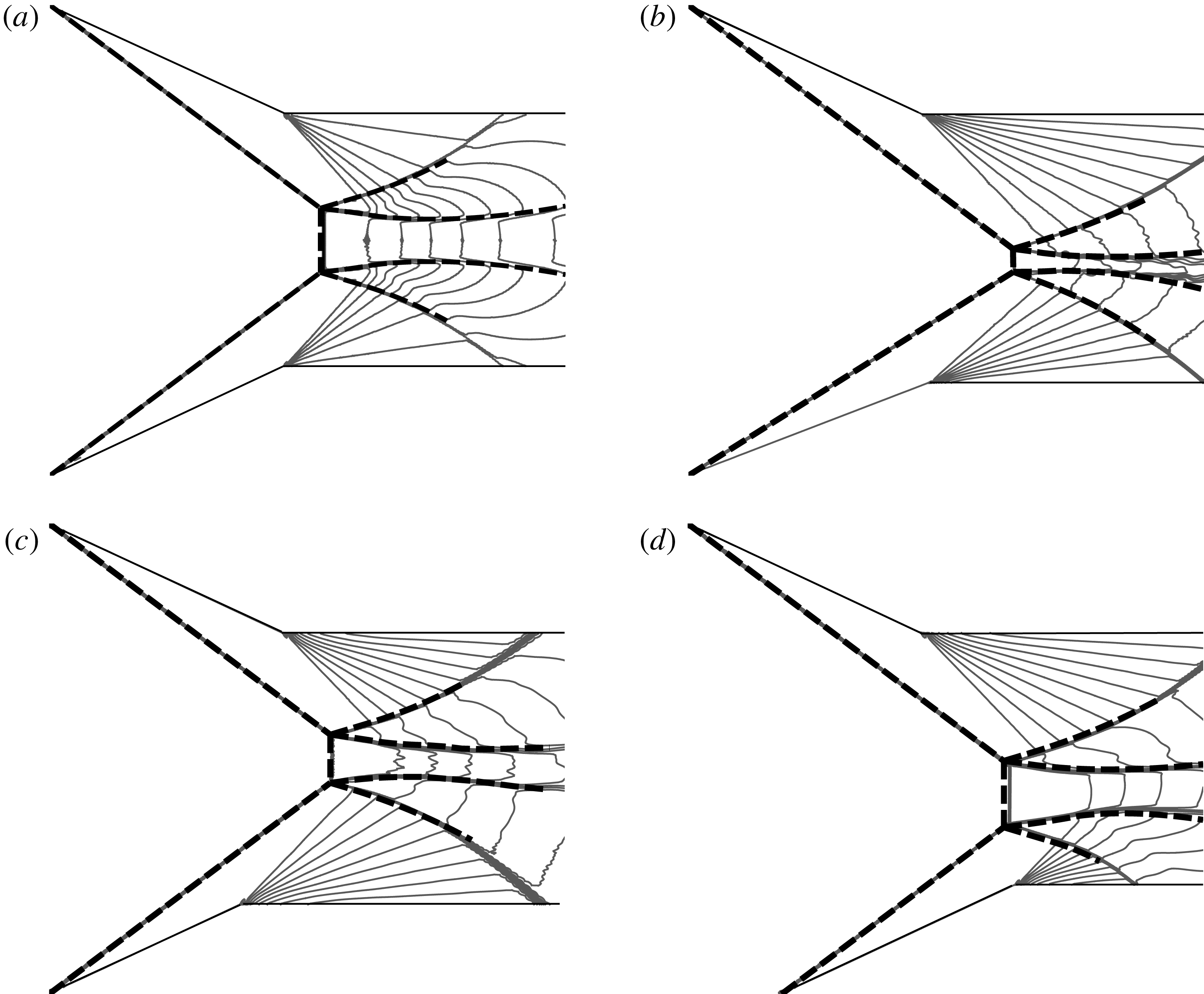
Analytical solution superimposed on the Mach number contours for various conditions at
 $M_{0}=4.5$
,
 $\unicode[STIX]{x1D703}_{w1}=25^{\circ }$
,
 $w_{1}/H_{A}=0.55$
. Grey lines are Mach number contour lines by CFD. Dashed lines are shock waves and sliplines by theory.

Similarly to Gao & Wu (Reference Gao and Wu2010) and Bai & Wu (Reference Bai and Wu2017) for symmetrical flow, here we show the overall flow configurations obtained by both theory and CFD. This allows us to see to what extent the theory can predict the shape of sliplines and various shock waves.
First we should verify whether the theory agrees well with CFD for symmetrical case. Figure 7(a) displays the flow under the symmetrical flow conditions
 $M_{0}=4.5$
,
 $\unicode[STIX]{x1D703}_{w1}=\unicode[STIX]{x1D703}_{w2}=25^{\circ }$
,
 $w_{1}/H_{A}=w_{2}/H_{A}=0.55$
,
 $d=0$
. A good agreement between theory and CFD results is observed, including the size and shape of shock waves and sliplines.
Now we consider asymmetrical flow cases. Figure 7(b) displays the flow with the same set of flow conditions as figure 7(a) except that with a different wedge angle for
 $\unicode[STIX]{x1D703}_{w2}$
. Here
 $\unicode[STIX]{x1D703}_{w2}=21^{\circ }\neq \unicode[STIX]{x1D703}_{w1}$
. The theory still agrees with the CFD result. Compared with the symmetrical reflection as shown in figure 7(a), the height of the Mach stem is reduced, due to the reduced
 $\unicode[STIX]{x1D703}_{w2}$
.
Figure 7(c) displays the flow with the same set of flow conditions as figure 7(a) except that the lower wedge length is reduced to
 $w_{2}/H_{A}=0.45$
. The height of the Mach stem is slightly reduced due to the reduced
 $w_{2}$
. The theory still compares well with CFD.
Figure 7(d) displays the flow with the same set of flow conditions as figure 7(a) except that there is a horizontal shift
 $d/H_{A}=0.2$
of the leading edge positions of the two wedges. The theory still compares well with CFD. Though the Mach stem height appears not to be obviously affected by this shift, the Mach stem is substantially deviated towards the wedge which is horizontally shift to the right side.
We have stated in § 2.2.1 that the sonic throat condition for asymmetrical reflection is different from the symmetrical case. The sonic throat occurs at a position given by (2.10) (see figure 5 for illustration), which means that the slopes of the two sliplines do not vanish at the same
 $z$
.
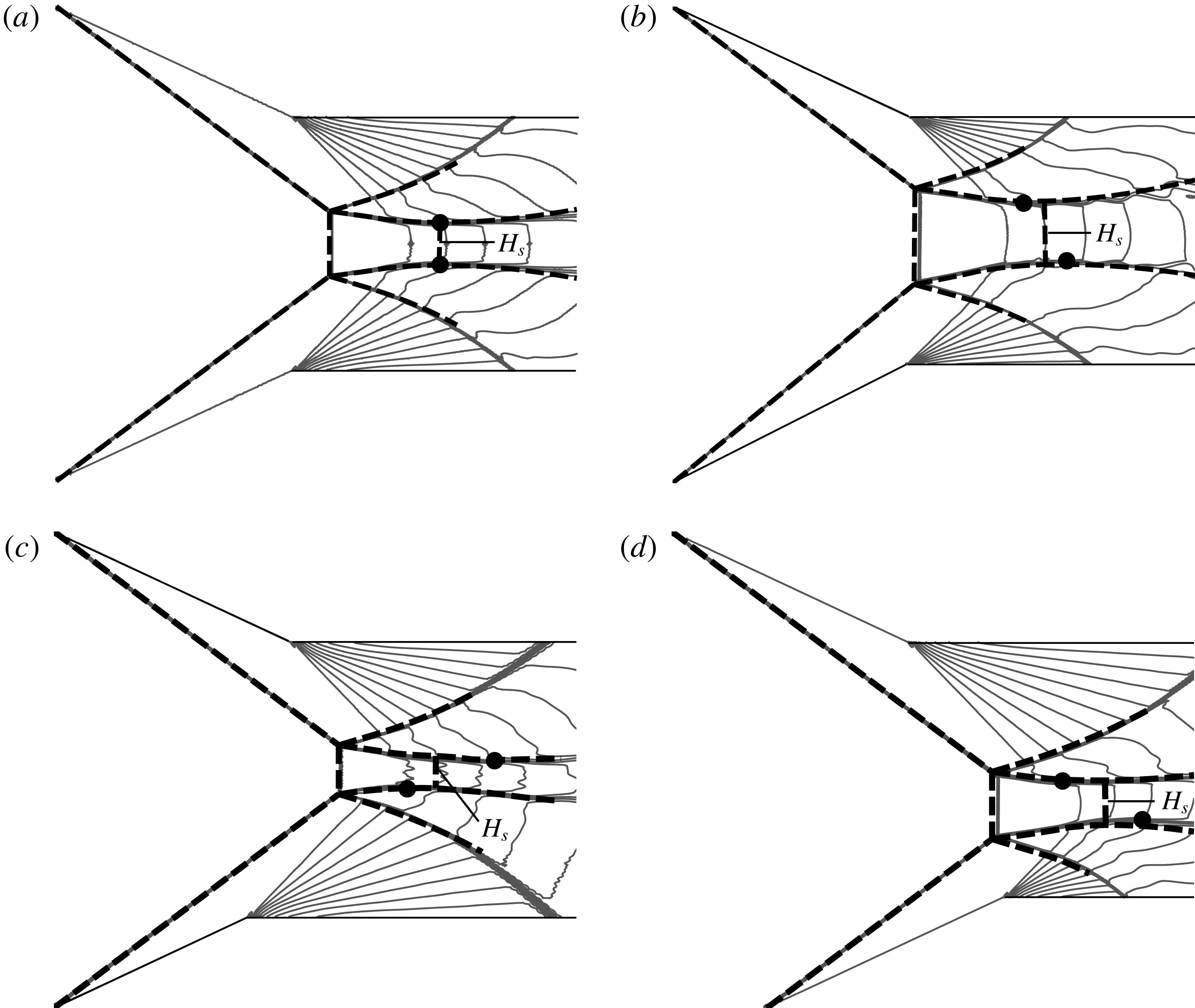
Prediction of the sonic throat of the flow duct for various conditions at
 $M_{0}=4.5$
,
 $\unicode[STIX]{x1D703}_{w1}=25^{\circ }$
,
 $w_{1}/H_{A}=0.55$
. Grey lines are Mach number contour lines by CFD, in which the sonic throat is marked with
 $M_{s}=M_{s}^{\ast }=1$
. Dashed lines are the sonic throat and flow structures predicted by theory. Solid dots are the points where the sliplines have vanishing slope.

Figure 8 displays the locations of sonic throat positions predicted by CFD and theory. Figure 8(a) shows that for symmetrical flow case, the sonic throat occurs at the positions where the slopes of the two sliplines vanish, a conclusion reached by Li & Ben-Dor (Reference Li and Ben-Dor1997).
Figure 8(b–d) shows the locations of sonic throat positions for an asymmetrical flow case. Figure 8(b) shows asymmetry in the wedge angles such that
 $\unicode[STIX]{x1D703}_{w2}=27^{\circ }\neq \unicode[STIX]{x1D703}_{w1}$
, figure 8(c) shows asymmetry in the wedge lengths such that
 $w_{2}/H_{A}=0.45\neq w_{1}/H_{A}$
and figure 8(d) shows asymmetry in the wedge horizontal position such that
 $d/H_{A}=0.2\neq 0$
. It is illustrated that the sonic throat locates between two points where either the lower or the upper slipline has vanishing slope. The theory compares well with CFD, for which we display the Mach contour with unit Mach number. This good comparison supports the sonic throat compatibility condition stated in § 2.2.4.
3.2 Effect of the wedge angle and length asymmetry on Mach stem size and shape
Now we consider the effect of asymmetry of the wedge angle and length on the size and shape of the Mach stem. The shape of the Mach stem has been assumed to be a circular arc. Here we are interested in the difference of the horizontal places of the two triple points
 $T_{1}(x_{T1},y_{T_{1}})$
and
 $T_{2}(x_{T2},x_{T2})$
, measured by the inclination angle
 $\unicode[STIX]{x1D6FD}_{m}$
of the Mach stem. This angle is defined by
 $$\begin{eqnarray}\tan \unicode[STIX]{x1D6FD}_{m}=\frac{y_{T2}-y_{T1}}{x_{T2}-x_{T1}}\end{eqnarray}$$
with
 $\unicode[STIX]{x1D6FD}_{m}<90^{\circ }$
for
 $x_{T1}>x_{T2}$
and
 $\unicode[STIX]{x1D6FD}_{m}>90^{\circ }$
for
 $x_{T1}<x_{T2}$
.
The size of the Mach stem is measured by
 $H_{m}=\sqrt{(x_{T1}-x_{T2})^{2}+(y_{T1}-y_{T2})^{2}}$
in CFD and is predicted theoretically by the method in § 2.3.
The Mach stem height for various conditions at
 $M_{0}=4.5$
,
 $\unicode[STIX]{x1D703}_{w1}=25^{\circ }$
,
 $w_{1}/H_{A}=0.55$
. Here the Mach stem height
 $H_{m}$
is normalized by
 $H_{A}$
.

3.2.1 Comparison between theory, CFD and experiments of previous studies
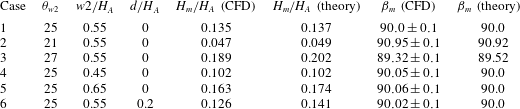
Table 1 displays the comparison of the theoretical and numerical results for several conditions. It is seen that comparison between theory, CFD and experiments of previous studies is overall acceptable, although the problem is complex and the model involves some simplified treatment. The discrepancy increases when asymmetry is amplified.
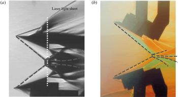
Analytical solution superimposed on the experimental results of (a) Sudani et al. (Reference Sudani, Sato, Karasawa, Noda, Tate and Watanabe2002) for
 $M_{0}=3$
,
 $\unicode[STIX]{x1D703}_{w1}=21^{\circ }$
,
 $\unicode[STIX]{x1D703}_{w2}=20.2^{\circ }$
,
 $H_{A}=201.9~\text{mm}$
,
 $w_{1}=w_{2}=127.9~\text{mm}$
,
 $d=0$
. (b) Li et al. (Reference Li, Chpoun and Ben-Dor1999) for
 $M_{0}=4.96$
,
 $\unicode[STIX]{x1D703}_{w1}=28^{\circ }$
,
 $\unicode[STIX]{x1D703}_{w2}=18^{\circ }$
,
 $H_{A}=71~\text{mm}$
,
 $w_{1}=w_{2}=40~\text{mm}$
,
 $d=0$
. Dashed lines are shock waves and sliplines by theory.

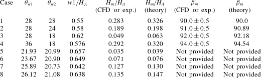
The comparison of the theory and CFD/experimental results of the height and the declined angle of the Mach stem (
 $w_{2}=w_{1}$
).

Table 2 shows comparison between theory and some known numerical and experimental results for symmetrical and asymmetrical configurations. The first four cases are CFD results from the numerical simulation of Kudryavstsev, Khotyanosky & Ivanov (Reference Kudryavstsev, Khotyanosky and Ivanov2000) for various conditions at
 $M_{0}=4.96$
,
 $d=0$
. The next four cases are the experimental results of Hornung & Mouton (Reference Hornung and Mouton2008), Mouton (Reference Mouton2008) and Mouton & Hornung (Reference Mouton and Hornung2008) for various conditions at
 $M_{0}=4$
. Note that some values of the inclination angle
 $\unicode[STIX]{x1D6FD}_{m}$
of the Mach stem are not provided in the above mentioned previous studies. Here the Mach stem height
 $H_{m}$
is normalized by
 $H_{A}$
. The agreement is still good enough, though the theoretical value is slightly larger than the numerical and experimental value for the Mach stem height.
Figure 9(a) displays analytical shapes of shock waves and sliplines superimposed on a schlieren photograph of an experiment by Sudani et al. (Reference Sudani, Sato, Karasawa, Noda, Tate and Watanabe2002) under the same condition and they agree well with each other, including the size and shape of shock waves and sliplines. Theory gives
 $H_{m}/H_{A}=0.103$
while experiment gives
 $H_{m}/H_{A}=0.102$
. Figure 9(b) displays the comparison between analytical solution and experimental results of Li et al. (Reference Li, Chpoun and Ben-Dor1999) under the same condition. The comparison is good for the position of Mach stem, while there is some discrepancy in the shape of the reflected shock wave of the lower side. This discrepancy is due to perturbation by the backside of the lower wedge which is too close to the reflected shock wave. Although theory does not account for viscous and three-dimensional effects, the comparison in both cases is acceptable. The influence of the viscous effect on the Mach stem height and flow structure has been studied by Schmisseur & Gaitonde (Reference Schmisseur and Gaitonde2011) and Guan, Bai & Wu (Reference Guan, Bai and Wu2018) for symmetrical reflection with two incident shock waves, showing that the flow structure is only slightly affected and the Mach stem height is slightly increased by viscosity. The effect of viscosity on the Mach stem height can be accounted for by adding a modification to the wedge angles and this modification is due to the displacement effect of the boundary layer developed over the wedge surfaces according to a separate study in progress. If the Reynolds number is large enough, the displacement thickness is small and the effect of viscosity on the Mach stem height is small.
We have seen in table 2 that the error in the prediction of Mach stem height is relatively large for cases 3 and 4, for the same reason as in the symmetrical case (Bai & Wu Reference Bai and Wu2017, § 3.2). Compared with case 2, the difference between the two wedge angles is larger for cases 3 and 4, leading to a larger slipline angle
 $\unicode[STIX]{x1D6FF}_{s1}^{T1}$
(defined in figure 5). In these cases, the secondary waves generated over the free part of the slipline are relatively strong so that the transmitted expansion waves should be more seriously disturbed by these secondary waves, which means the utilization of regularized transmitted expansion waves rather than curved Mach waves would be less accurate for higher
 $\unicode[STIX]{x1D6FF}_{s1}^{T1}$
or
 $\unicode[STIX]{x1D6FF}_{s2}^{T2}$
. A future study to improve the accuracy of the present model would involve the improvement of the regularized transmitted expansion wave model.
3.2.2 Influence of the asymmetry of the wedge angles and lengths
Now, we study how the Mach stem height
 $H_{m}$
and the reduced declination angle
 $\unicode[STIX]{x1D6FF}=\unicode[STIX]{x1D6FD}_{m}-90^{\circ }$
(measure of deviation from the vertical axis) of the Mach stem are affected by the asymmetry of the wedge angles and lengths.
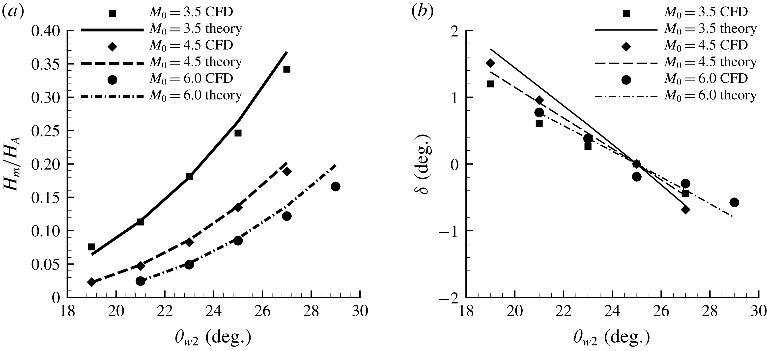
Influence of the asymmetry of wedge angles by varying
 $\unicode[STIX]{x1D703}_{w2}$
(
 $\unicode[STIX]{x1D703}_{w1}=25^{\circ }$
,
 $w_{1}/H_{A}=w_{2}/H_{A}=0.55$
,
 $d=0$
). (a) Mach stem height, (b) reduced declined angle
 $\unicode[STIX]{x1D6FF}$
of the Mach stem.

First consider the asymmetry of wedge angles (
 $\unicode[STIX]{x1D703}_{w1}\neq \unicode[STIX]{x1D703}_{w2}$
), with equal wedge lengths. As shown in figure 10, where both theory and CFD data are displayed, if the upper wedge angle
 $\unicode[STIX]{x1D703}_{w1}$
is fixed, the Mach stem height
 $H_{m}$
grows rapidly for increasing
 $\unicode[STIX]{x1D703}_{w2}$
, and the reduced declination angle
 $\unicode[STIX]{x1D6FF}$
of the Mach stem decrease from
 $\unicode[STIX]{x1D6FF}>0$
to
 $\unicode[STIX]{x1D6FF}<0$
with
 $\unicode[STIX]{x1D703}_{w2}$
increasing from
 $\unicode[STIX]{x1D703}_{w2}<\unicode[STIX]{x1D703}_{w1}$
to
 $\unicode[STIX]{x1D703}_{w2}>\unicode[STIX]{x1D703}_{w1}$
. It can be seen that the agreement between theory and CFD results is better for smaller values of
 $\unicode[STIX]{x1D703}_{w2}$
and becomes worse as
 $\unicode[STIX]{x1D703}_{w2}$
increases, and the reason for this has been stated above on explaining the larger discrepancy of cases 3 and 4 of table 2.
Let us explain the reason for these observations. When
 $\unicode[STIX]{x1D703}_{w2}$
increases, the slipline angle
 $\unicode[STIX]{x1D6FF}_{s2}$
also increases by the three-shock theory for triple point
 $T_{2}$
, and the flow duct between the sliplines is more convergent along the flow direction. This means that the sonic condition
 $M_{s}=M_{s}^{\ast }=1$
occurs earlier and the pressure drops faster in the duct. Thus the Mach stem height must increase to balance the pressure drop from the regions of transmitted expansion waves.
According to figure 4 of Tan et al. (Reference Tan, Ren and Wu2006), the initial slipline angle at a triple point grows fast when the wedge deflection angle increases. Thus the slipline angle
 $\unicode[STIX]{x1D6FF}_{s2}$
grows fast when
 $\unicode[STIX]{x1D703}_{w2}$
increases. Since the height of sonic throat, which depends strongly on
 $\unicode[STIX]{x1D6FF}_{s2}$
, is related to
 $H_{s}^{\ast }/H_{m}$
, the Mach stem height grows very fast when
 $\unicode[STIX]{x1D6FF}_{s2}$
increases.
As shown in (2.4), the tangents of the Mach stem at the triple points
 $T_{1}$
and
 $T_{2}$
equal
 $\unicode[STIX]{x1D6FD}_{m}^{T1}$
and
 $\unicode[STIX]{x1D6FD}_{m}^{T2}$
. If the angle of wedges
 $\unicode[STIX]{x1D703}_{w1}>\unicode[STIX]{x1D703}_{w2}$
, then
 $|\unicode[STIX]{x1D6FD}_{m}^{T1}|<|\unicode[STIX]{x1D6FD}_{m}^{T2}|$
and
 $x_{T1}<x_{T2}$
according to the three-shock theory and geometrical relation, as a result
 $\unicode[STIX]{x1D6FD}_{m}>90^{\circ }$
and
 $\unicode[STIX]{x1D6FF}>0$
. Similarly, if
 $\unicode[STIX]{x1D703}_{w1}<\unicode[STIX]{x1D703}_{w2}$
,
 $\unicode[STIX]{x1D6FD}_{m}<90^{\circ }$
and
 $\unicode[STIX]{x1D6FF}<0$
.
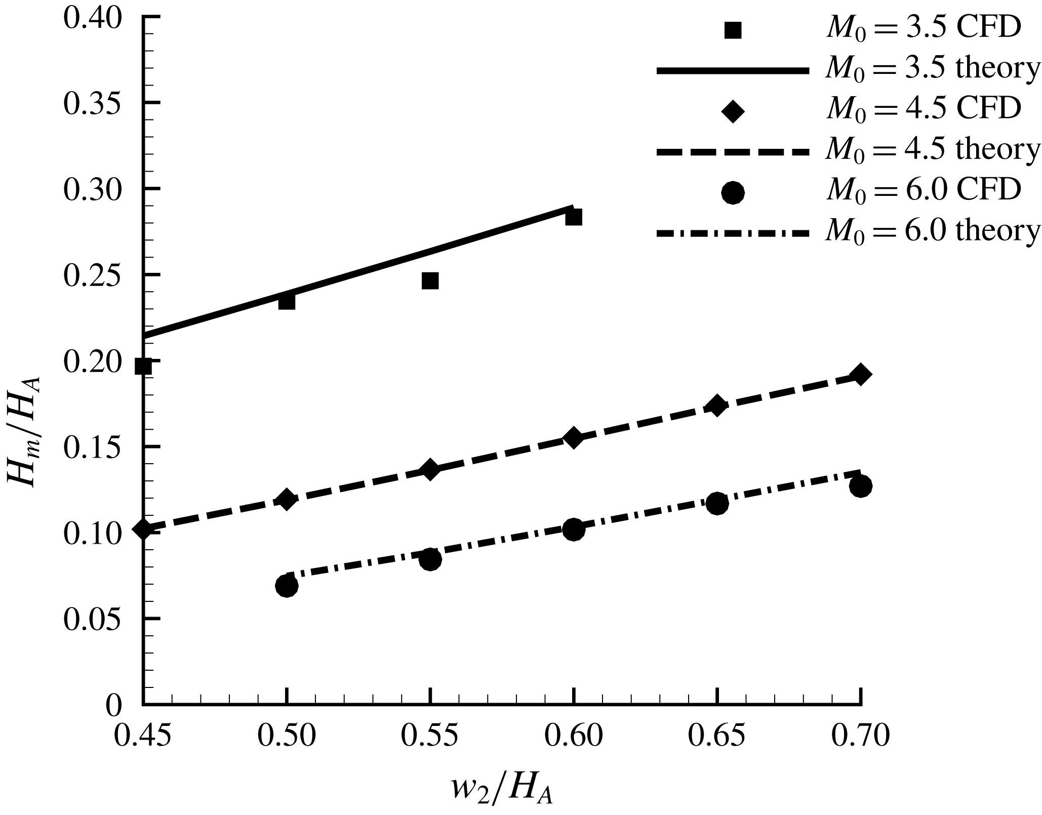
Influence of the asymmetry of the wedge length on the Mach stem height by varying
 $w_{2}$
(
 $\unicode[STIX]{x1D703}_{w1}=\unicode[STIX]{x1D703}_{w2}=25^{\circ }$
,
 $w_{1}/H_{A}=0.55$
,
 $d=0$
).

Now consider the asymmetry of wedge length (
 $w_{1}\neq w_{2}$
). This leads to asymmetry of the rear corners of wedges (
 $x_{R1}\neq x_{R2}$
), which produces asymmetrical expansion fans
 $R_{c1}$
and
 $R_{c2}$
and leads to the asymmetry in the overall shock reflection. As shown in figure 11, the Mach stem height grows almost linearly when the lower wedge length
 $w_{2}/H_{A}$
increases. Note that this asymmetry does not influence the shock angle of the Mach stem
 $\unicode[STIX]{x1D6FD}_{m}$
.
When the length of lower wedge
 $w_{2}/H_{A}$
increases with other conditions fixed, the rear corner of the lower wedge
 $R_{2}$
and the expansion fan
 $R_{c2}$
moves towards the upper right (see figure 5). Thus the turning point
 $B_{2}$
moves downstream. It can then be argued that the Mach stem height must increase almost linearly for the pressure balance between the convergent duct and the region of transmitted expansion waves from the lower wedge. As the Mach number of the flow behind the Mach stem
 $M_{m}$
and the slipline angle
 $\unicode[STIX]{x1D6FF}_{s2}^{T2}$
solved by three-shock theory are unaffected by varying the lower wedge length
 $w_{2}$
, the ratio of the height of the sonic throat and the Mach stem height
 $H_{s}^{\ast }/H_{m}$
should remain the same according to one-dimensional isentropic flow theory. As
 $T_{2}B_{2}$
is slightly curved and can be treated as a straight line with fixed slope
 $\unicode[STIX]{x1D6FF}_{s2}^{T2}$
, points
 $T_{2}$
and
 $B_{2}$
must move the same vertical distance, leading to the nearly linear growth of the Mach stem in order to keep
 $H_{s}^{\ast }/H_{m}$
unchanged.
As the asymmetry in the length of the wedges does not affect
 $\unicode[STIX]{x1D6FD}_{m}^{T1}$
and
 $\unicode[STIX]{x1D6FD}_{m}^{T2}$
, the overall shock angle
 $\unicode[STIX]{x1D6FD}_{m}$
of the Mach stem remains the same.
3.3 The asymmetrical effect caused by horizontal shift of the wedges
The horizontal shift of the wedges is measured by
 $d=x_{A2}-x_{A1}$
. As shown above, the reduced declination angle
 $\unicode[STIX]{x1D6FF}$
of the Mach stem is only dependent of the asymmetry of the wedge angles so that it is not changed by purely varying
 $d$
.
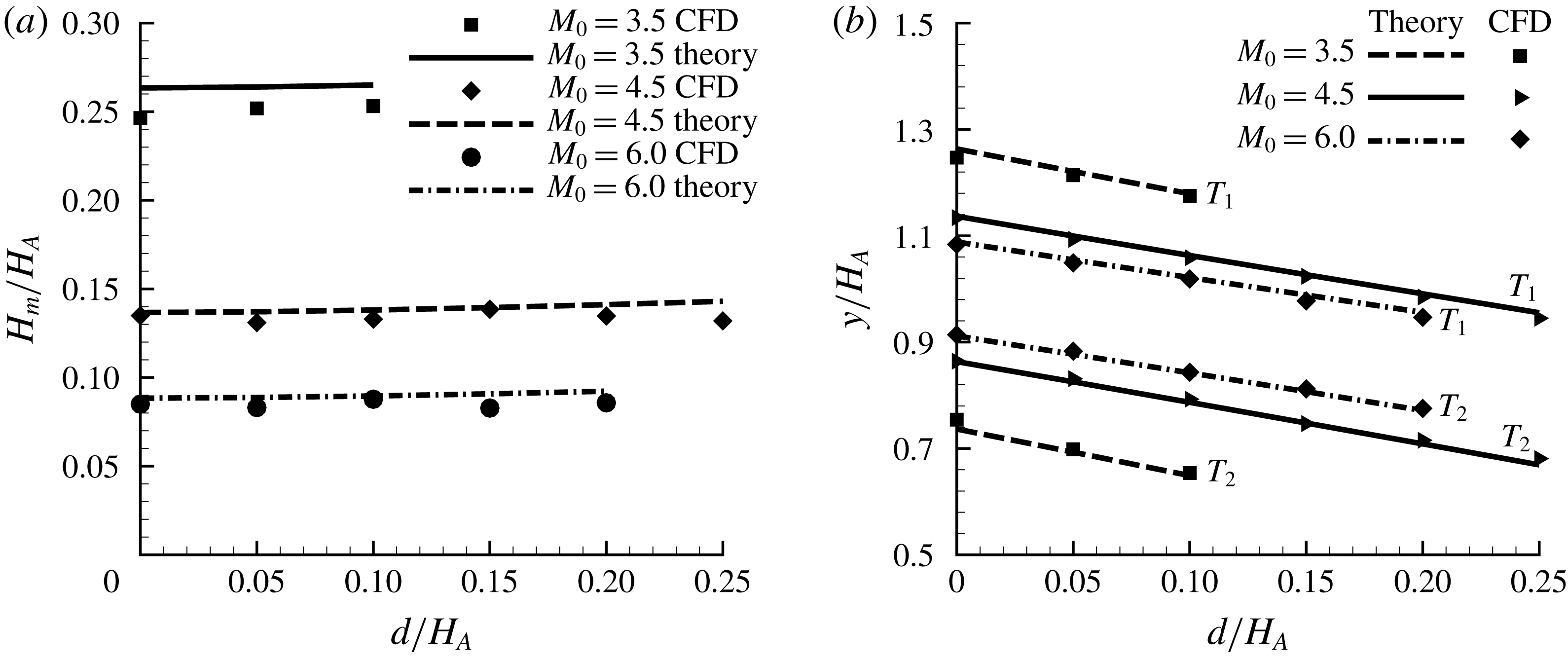
Influence of horizontal shift
 $d$
(
 $\unicode[STIX]{x1D703}_{w1}=\unicode[STIX]{x1D703}_{w2}=25^{\circ }$
,
 $w_{1}/H_{A}=w_{2}/H_{A}=0.55$
). (a) Mach stem height, (b) vertical locations of triple points
 $T_{1}$
and
 $T_{2}$
.

Figure 12(a) displays the Mach stem heights as a function of
 $d$
, obtained by both CFD and theory. It is seen that the Mach stem height grows only slightly with increasing
 $d$
, meaning that the Mach stem height is insensitive to the horizontal shift of the wedge. Figure 12(b) displays the vertical locations of the two triple points. The two vertical locations of both triple points move downstream when
 $d$
increases.
Let us first explain why the two triple points (and thus Mach stem) move downstream when there is a horizontal shift. It is easily understandable that if both leading edges
 $A_{1}$
and
 $A_{2}$
of the wedge (see figure 5) were allowed to move downstream, then all the flow structures also move downstream. Thus it is also understandable that if only
 $A_{2}$
moves downstream to have increasing
 $d$
, then the lower part of the flow structures (such as the lower triple point, lower slipline and lower reflected shock wave) also move downstream. However, the Mach stem reduced declination angle
 $\unicode[STIX]{x1D6FF}$
(defined in § 3.2.2) is unaffected by changing
 $d$
, for the reason discussed in § 3.2.2. Thus, when
 $d$
increases, the rear corner
 $R_{2}$
and the expansion fan
 $R_{c2}$
of the lower wedge move towards right (see figure 5). This means that the turning point
 $B_{2}$
, which lies on the leading characteristics of
 $R_{c2}$
, also moves downstream. As a result, both triple points must move downstream for increasing
 $d$
, to balance the pressure between the duct flow and expansion waves from the lower wedge rear corner.
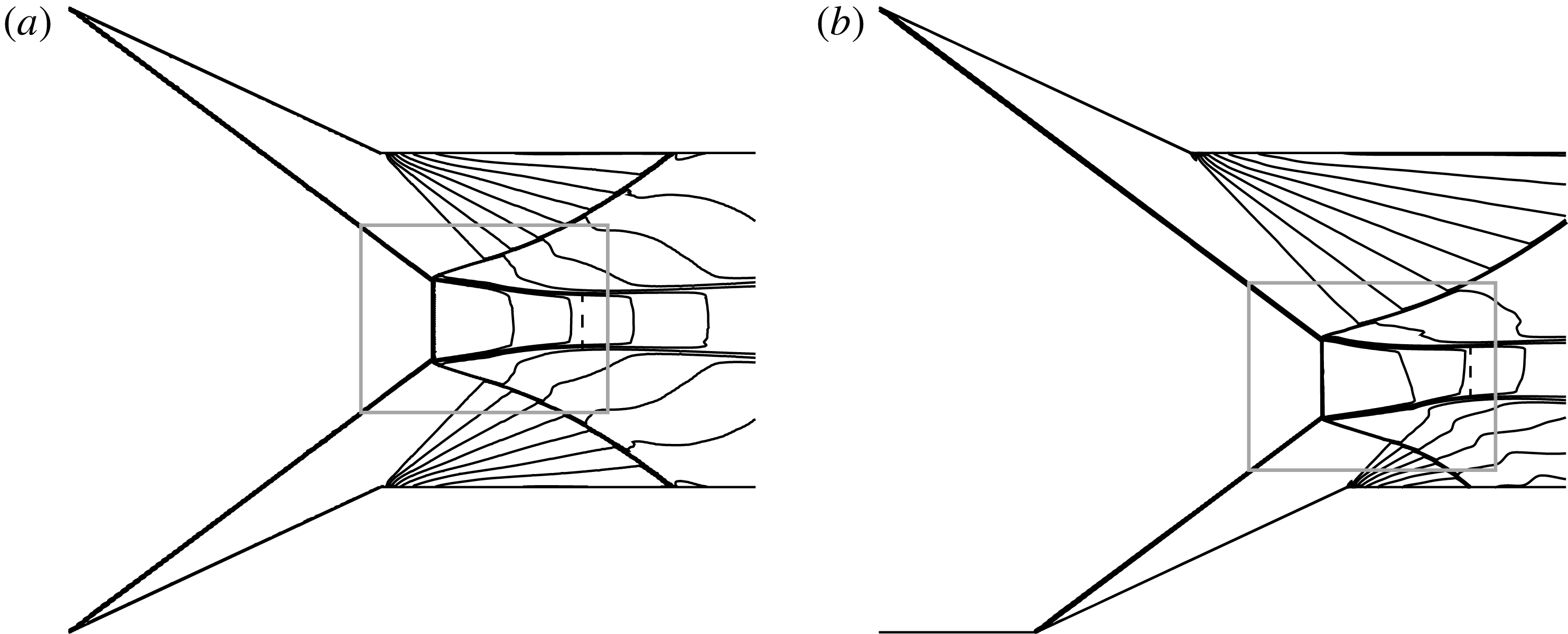
Mach contours for varying horizontal shift (a)
 $d=0$
, (b)
 $d=0.25H_{A}$
. The other conditions are the same and are given by
 $M_{0}=4.5$
,
 $\unicode[STIX]{x1D703}_{w1}=\unicode[STIX]{x1D703}_{w2}=25^{\circ }$
,
 $w_{1}/H_{A}=w_{2}/H_{A}=0.55$
.

The insensitivity of the Mach stem height to the horizontal shift would imply some close similarity of the flow structures for various
 $d$
. To see this we display in figure 13 Mach contours for
 $d=0$
and
 $0.25H_{A}$
. To check this, we first postulate a geometrical similarity: when
 $d$
increases, the Mach stem and the reflected shock waves and sliplines move to a downstream position while keeping their shape and size. Assuming the Mach stem height remains unchanged, and using the condition that the upper triple point lies on the upper incident shock wave, it can be easily checked, using a geometrical relationship, that a reference point (such as the middle point) of the Mach stem should move right by a distance of
 $d\sin \unicode[STIX]{x1D6FD}_{i2}\cos \unicode[STIX]{x1D6FD}_{i1}/\text{sin}(\unicode[STIX]{x1D6FD}_{i1}+\unicode[STIX]{x1D6FD}_{i2})$
, and move down by a distance of
 $d\sin \unicode[STIX]{x1D6FD}_{i2}\,\text{sin}\unicode[STIX]{x1D6FD}_{i1}/\text{sin}(\unicode[STIX]{x1D6FD}_{i1}+\unicode[STIX]{x1D6FD}_{i2})$
.
We draw a box in figure 13(a) and then draw another box in figure 13(b) which is on the bottom right of the first one, and their horizontal and vertical distances satisfy
 $d\sin \unicode[STIX]{x1D6FD}_{i2}\cos \unicode[STIX]{x1D6FD}_{i1}/\text{sin}(\unicode[STIX]{x1D6FD}_{i1}+\unicode[STIX]{x1D6FD}_{i2})$
and
 $d\sin \unicode[STIX]{x1D6FD}_{i2}\sin \unicode[STIX]{x1D6FD}_{i1}/\text{sin}(\unicode[STIX]{x1D6FD}_{i1}+\unicode[STIX]{x1D6FD}_{i2})$
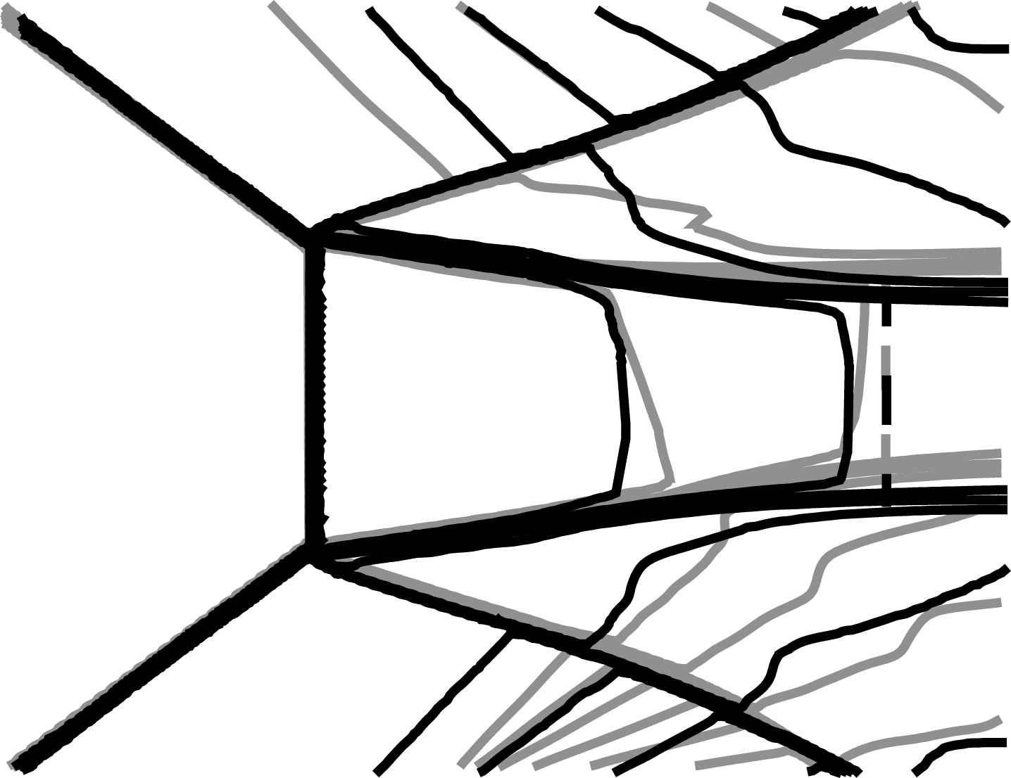
. The flow structures inside the boxes (which have the same size and which are located at different positions) are superimposed in figure 14.
The superimposed Mach number contours from the flow structures inside the boxes displayed in figure 13, showing close similarity of the flow structures inside the boxes. The dark contour is from figure 13(a) and the grey one is from figure 13(b). The dashed line is the Mach contour with unit Mach number.

It is seen that the flow structures inside the two boxes are indeed very similar, i.e. the shapes and positions of the Mach stem, reflected shock waves and sliplines before the sonic throat are almost the same for
 $d=0$
and
 $0.25H_{A}$
, except that their positions have a shift.
If there were exact similarity, then all the mechanisms (exactly the same oblique shock and leading expansion fan characteristic, the characteristics that intersect the slipline before the sonic throat) determining the Mach stem height would be exactly the same when
 $d$
changes. However, the similarity, as shown in figure 14, is only approximate, so that the Mach stem height changes weakly with
 $d$
.
4 Concluding remarks
In this paper an analytical model is built to study the overall flow structure for asymmetrical shock wave reflections. This model is updated from the symmetrical model of Bai & Wu (Reference Bai and Wu2017) to account for the new features of asymmetrical reflection. A new sonic throat compatibility condition is built and verified for asymmetrical Mach reflection. The asymmetry includes the difference of wedge angles, wedge lengths and positions of the wedge leading edges. The theory compares well with CFD results.
Both theory and CFD are used to study the effect of wedge asymmetry on the flow structure, Mach stem height and shape, as well as the shape of reflected shock waves and sliplines. Below are the main conclusions.
The Mach stem height is strongly affected by the asymmetry of the wedge angles, which grows superlinearly for an increase in one wedge angle with the other one fixed.
The reduced declination angle (measure as the deviation from the vertical axis) of the Mach stem is only affected by the asymmetry of the wedge angles. The asymmetry of the wedge lower surface length or horizontal shift of the wedges does not change the orientation of the Mach stem.
The Mach stem height is affected almost in a linear way by the asymmetry of the wedge lengths. Keeping one wedge length fixed, the Mach stem height increases almost linearly with the other wedge length.
The influence of the asymmetry of the horizontal positions of the wedges is subtle. The Mach stem height is almost independent of (weakly increasing with) the horizontal shift of the leading edge of one wedge with respect to the other. However, the Mach stem moves downward and toward the side of the wedge that is shifted to the right-hand side. It is demonstrated that the flow structure near the Mach stem is almost similar when there is a horizontal shift of either wedge.
Acknowledgements
The referees and associate editor have provided many helpful comments to improve the content and style of the paper. The authors wish to express their great thanks to them. This work was supported by the Natural National Science Foundation of China (no. 11802157).
Appendix A. Details of the global model for asymmetrical Mach reflection
The models in §§ A.1 and A.2 are independent of the Mach stem and are computed first. Section A.3 starts an iteration process for finding the Mach stem height and for computing the shape and positions of the Mach stem, reflected shock waves and sliplines.
A.1 Incident shock wave solution and triple point solution
These solutions are independent of the Mach stem height. Applying the oblique shock wave relations to the two incident shock waves gives the shock angles
 $\unicode[STIX]{x1D6FD}_{i1}$
and
 $\unicode[STIX]{x1D6FD}_{i2}$
, as well as uniform flow solutions in regions
 $1$
and
 $7$
(including pressure
 $p_{1},p_{7}$
, Mach number
 $M_{1},M_{7}$
and Mach angles
 $\unicode[STIX]{x1D707}_{1}=\arcsin (1/M_{1})$
and
 $\unicode[STIX]{x1D707}_{7}=\arcsin (1/M_{7})$
). Applying the triple point theory of von Neumann to each triple points gives the triple point solutions, including the slipline deflection angles (
 $\unicode[STIX]{x1D6FF}_{s1}^{T1}$
,
 $\unicode[STIX]{x1D6FF}_{s2}^{T2}$
) and shock angles (
 $\unicode[STIX]{x1D6FD}_{r1}^{T1},\unicode[STIX]{x1D6FD}_{r2}^{T2}$
) at the triple points, the near-triple point strong shock wave solutions (
 $p_{3}^{T1}$
,
 $M_{3}^{T1}$
,
 $p_{9}^{T2}$
,
 $M_{9}^{T2}$
just downstream of the Mach stem) and the near-triple point weak shock solutions (
 $p_{2}^{T1}$
,
 $M_{2}^{T1}$
,
 $p_{8}^{T2}$
,
 $M_{8}^{T2}$
just downstream of the reflected shock waves). The arithmetic averages
 $$\begin{eqnarray}\left.\begin{array}{@{}c@{}}p_{s}(0)=p_{m}={\textstyle \frac{1}{2}}\left({\textstyle \frac{1}{2}}(p_{3}^{T1}+p_{9}^{T2})+p_{g}\right)\\ M_{s}(0)=M_{m}={\textstyle \frac{1}{2}}\left({\textstyle \frac{1}{2}}(M_{3}^{T1}+M_{9}^{T2})+M_{g}\right)\end{array}\right\}\end{eqnarray}$$
are used as the inlet condition of the quasi-one-dimensional flow model. Here
 $M_{g}$
,
 $p_{g}$
are normal shock wave solutions, using the inflow stream condition.
A.2 Initial guess of the Mach stem height and positions of triple points
Given a Mach stem height
 $H_{m}$
which is initially guessed in the first round of iteration (using the method of Li & Ben-Dor (Reference Li and Ben-Dor1997) as discussed below) and adapted in the end of each round of iteration, we compute the triple point positions
 $(x_{T1},y_{T1})$
and
 $(x_{T2},y_{T2})$
using the relations (2.2)–(2.4).
Now we briefly describe how to find an initial guess of the Mach stem height. The initial guess is given as
 $$\begin{eqnarray}H_{m}={\textstyle \frac{1}{2}}(H_{m,max}+H_{m,min}),\end{eqnarray}$$
where
 $H_{m,max}$
and
 $H_{m,min}$
are possible maximum and minimum heights of the assumed Mach stem. Li & Ben-Dor (Reference Li and Ben-Dor1997) give a method to estimate these heights for symmetrical Mach reflection. Specifically, they provided expressions for estimating the most upstream and downstream positions of the triple point and the maximum and minimum Mach stem heights follow from these positions.
Here, we estimate these most upstream and downstream positions of each triple point for each of the wedge configurations in a similar way as for symmetrical reflection and determine
 $H_{m,max}$
and
 $H_{m,min}$
as their distances.
A.3 Loop of iteration
Once the Mach stem height is initially guessed or updated in § A.6, the shapes of the reflected shock waves and sliplines are computed, using the algorithms detailed in §§ A.4 and A.5.
A.4 Model for the shape of reflected shock waves shape
The reflected shock waves
 $r_{1}$
and
 $r_{2}$
are each divided into a free part (before the points
 $F_{1}$
and
 $F_{2}$
) and an interacting part (starting from
 $F_{1}$
and
 $F_{2}$
). The points
 $F_{1}$
and
 $F_{2}$
are the intersection of the reflected shock waves and the leading characteristics of the wedge corner expansion fan.
(a) Free part of reflected shock waves
As in Bai & Wu (Reference Bai and Wu2017), the free parts are assumed to be straight, so that their slopes are uniquely determined by their shock angles
 $\unicode[STIX]{x1D6FD}_{r1}^{T1}$
and
 $\unicode[STIX]{x1D6FD}_{r2}^{T2}$
at the triple points. The slopes of the leading characteristics of the two expansion fans are determined by the Mach angle
 $\unicode[STIX]{x1D707}_{1}$
and
 $\unicode[STIX]{x1D707}_{7}$
. Thus, the positions of
 $F_{1}$
and
 $F_{2}$
can be determined by the following obvious geometric relations
 $$\begin{eqnarray}\left.\begin{array}{@{}c@{}}y_{F1}-y_{T1}=(x_{F1}-x_{T1})\tan (\unicode[STIX]{x1D6FD}_{r1}^{T1}-\unicode[STIX]{x1D703}_{w1}),\\ y_{F1}-y_{R1}=-(x_{F1}-x_{R1})\tan (\unicode[STIX]{x1D707}_{1}+\unicode[STIX]{x1D703}_{w1}),\\ y_{F2}-y_{T2}=(x_{F2}-x_{T2})\tan (\unicode[STIX]{x1D703}_{w2}-\unicode[STIX]{x1D6FD}_{r2}^{T2}),\\ y_{F2}-y_{R2}=(x_{F2}-x_{R2})\tan (\unicode[STIX]{x1D707}_{7}+\unicode[STIX]{x1D703}_{w2}).\end{array}\right\}\end{eqnarray}$$
(b) Interacting parts of reflected shock waves
 $F_{1}K_{1}$
,
 $F_{2}K_{2}$
are the interacting parts of the reflected shock wave, which start from
 $F_{1}$
and
 $F_{2}$
separately. The shock shape for the symmetrical case has been studied for instance by Li & Ben-Dor (Reference Li and Ben-Dor1996) and Bai & Wu (Reference Bai and Wu2017). The analytical expression for the shock shape derived by Bai & Wu (Reference Bai and Wu2017) is obtained by the shock relation and characteristic theory. For the asymmetrical case, the mechanism to determine the shape of the reflected shock wave is the same as for the symmetrical case, so that the analytical expressions derived by Bai & Wu (Reference Bai and Wu2017) can be directly used for the shape of the interacting part of each reflected shock wave.
Following the final expressions given in § 2.2.1 of Bai & Wu (Reference Bai and Wu2017), the shape of the reflected shock waves (
 $i=1$
is for shock
 $r_{1}$
and
 $i=2$
for shock
 $r_{2}$
) in terms of the shock angles
 $\unicode[STIX]{x1D6FD}_{r1}$
and
 $\unicode[STIX]{x1D6FD}_{r2}$
can be directly expressed as
 $$\begin{eqnarray}\frac{\text{d}\unicode[STIX]{x1D6FD}_{ri}}{\text{d}\unicode[STIX]{x1D703}_{fi}}=-\frac{(\unicode[STIX]{x1D6FD}_{\unicode[STIX]{x1D703}i}-K_{5,i}\unicode[STIX]{x1D6FD}_{Mi})-\unicode[STIX]{x1D6FD}_{\unicode[STIX]{x1D703}i}K_{4,i}K_{3,i}}{1+2\times (-1)^{i+1}\unicode[STIX]{x1D6FD}_{\unicode[STIX]{x1D703}i}K_{4,i}\sin (2\unicode[STIX]{x1D6FD}_{ri})},\quad \unicode[STIX]{x1D6FD}_{ri}=\unicode[STIX]{x1D6FD}_{ri}^{Ti}\text{ at }\unicode[STIX]{x1D703}_{fi}=(-1)^{i}\unicode[STIX]{x1D703}_{wi},i=1,2,\end{eqnarray}$$
where
 $$\begin{eqnarray}\left.\begin{array}{@{}c@{}}\unicode[STIX]{x1D6FD}_{\unicode[STIX]{x1D703}i}=[1-K_{1,i}+2K_{2,i}M_{fi}\cos ^{2}\unicode[STIX]{x1D6FD}_{ri}],\\ \unicode[STIX]{x1D6FD}_{Mi}=(-1)^{i}[1-K_{1,i}+2K_{2,i}\cos ^{2}\unicode[STIX]{x1D6FD}_{ri}]^{-1}K_{2,i}\sin (2\unicode[STIX]{x1D6FD}_{ri}),\\ K_{1,i}={\displaystyle \frac{\sin (2(\unicode[STIX]{x1D6FD}_{ri}+\unicode[STIX]{x1D703}_{fi}-\unicode[STIX]{x1D703}_{ti}))}{\sin (2\unicode[STIX]{x1D6FD}_{ri})}},\quad K_{2,i}={\displaystyle \frac{2(\unicode[STIX]{x1D6FE}+1)M_{fi}\sin ^{2}(\unicode[STIX]{x1D6FD}_{ri}-\unicode[STIX]{x1D703}_{fi}+\unicode[STIX]{x1D703}_{ti})}{[(\unicode[STIX]{x1D6FE}-1)M_{fi}^{2}\sin ^{2}\unicode[STIX]{x1D6FD}_{ri}+2]}},\\ \unicode[STIX]{x1D703}_{ti}=\unicode[STIX]{x1D703}_{fi}+\arctan \left(2\cot \unicode[STIX]{x1D6FD}_{ri}{\displaystyle \frac{M_{fi}^{2}\sin ^{2}\unicode[STIX]{x1D6FD}_{ri}-1}{M_{fi}^{2}(\unicode[STIX]{x1D6FE}+\cos 2\unicode[STIX]{x1D6FD}_{ri}+2)}}\right),\\ K_{5,i}={\displaystyle \frac{M_{fi}}{\sqrt{M_{fi}^{2}-1}}}\unicode[STIX]{x1D717}(M_{fi}),\\ \unicode[STIX]{x1D717}(M)=1+{\displaystyle \frac{\unicode[STIX]{x1D6FE}-1}{2}}M^{2}.\end{array}\right\}\end{eqnarray}$$
In (A 4),
 $\unicode[STIX]{x1D703}_{f1}$
and
 $\unicode[STIX]{x1D703}_{f2}$
are the deflection angles of the flow direction inside the upper and lower wedge expansion fans
 $R_{c1}$
and
 $R_{c2}$
. They take the initial values
 $\unicode[STIX]{x1D703}_{f1}=-\unicode[STIX]{x1D703}_{w1}$
and
 $\unicode[STIX]{x1D703}_{f2}=\unicode[STIX]{x1D703}_{w2}$
, for the leading characteristics
 $R_{1}F_{1}$
and
 $R_{2}F_{2}$
.
The Mach number
 $M_{fi}$
and the pressure
 $p_{fi}$
in the two expansion fans are given by the Prandtl–Meyer flow solution.
The abscissae
 $x_{r1},x_{r2}$
on the reflected shock waves
 $F_{1}K_{1},F_{2}K_{2}$
are connected to
 $\unicode[STIX]{x1D703}_{f1}$
and
 $\unicode[STIX]{x1D703}_{f2}$
through pure geometrical relations. Following Bai & Wu (Reference Bai and Wu2017) for details, these abscissae meet the following expression
 $$\begin{eqnarray}\frac{\text{d}x_{ri}}{\text{d}\unicode[STIX]{x1D703}_{fi}}=\frac{1-M_{fi}^{2}-\unicode[STIX]{x1D717}(M_{fi})}{M_{fi}^{2}-1}\frac{(-1)^{i+1}(\tan ^{2}(\unicode[STIX]{x1D703}_{fi}-\unicode[STIX]{x1D707}_{fi})+1)}{\tan (\unicode[STIX]{x1D6FD}_{ri}-\unicode[STIX]{x1D703}_{fi})+\tan (-\unicode[STIX]{x1D703}_{fi}+\unicode[STIX]{x1D707}_{fi})}(x_{ri}-x_{Ri}),\quad i=1,2,\end{eqnarray}$$
where
 $\unicode[STIX]{x1D707}_{fi}=\arcsin (1/M_{fi})$
is the Mach angle at
 $M_{fi}$
.
Starting from point
 $F_{1}$
and
 $F_{2}$
, solve (A 4), (A 6) and
 $\text{d}y_{ri}/\text{d}x_{ri}=\tan (\unicode[STIX]{x1D6FD}_{ri}+\unicode[STIX]{x1D703}_{fi}),i=1,2$
to find
 $\unicode[STIX]{x1D6FD}_{r1}(\unicode[STIX]{x1D703}_{f1})$
and
 $\unicode[STIX]{x1D6FD}_{r2}(\unicode[STIX]{x1D703}_{f2})$
and the positions
 $G_{1}(x_{r1},y_{r1})$
and
 $G_{2}(x_{r2},y_{r2})$
of the reflected shock waves.
(c) Flow parameters downstream of reflected shock waves
Once the local shock angles are given, the use of oblique shock wave relations gives the downstream pressure (
 $p_{t1},p_{t2}$
) and Mach number (
 $M_{t1},M_{t2}$
), on the opposite sides of the shock waves with respect to the expansion fans
 $R_{c1}$
and
 $R_{c2}$
.
Since it will be the pressure gradient balance condition (2.8) to be used for finding the shape of the sliplines, we will need in the following the expressions for
 $\text{d}p_{ti}/\text{d}\unicode[STIX]{x1D703}_{fi}$
. For the symmetrical case, this is given by Bai & Wu (Reference Bai and Wu2017). When directly applied to the present case, we get
 $$\begin{eqnarray}\left.\begin{array}{@{}c@{}}{\displaystyle \frac{\text{d}p_{ti}}{\text{d}\unicode[STIX]{x1D703}_{fi}}}=(-1)^{i}(K_{6,i}+K_{7,i}){\displaystyle \frac{\unicode[STIX]{x1D6FE}p_{fi}M_{fi}^{2}}{\unicode[STIX]{x1D6FE}+1}},\\ K_{6,i}={\displaystyle \frac{1-\unicode[STIX]{x1D6FE}-2\sin ^{2}\unicode[STIX]{x1D6FD}_{r}(2-M_{fi}^{2})}{\sqrt{M_{fi}^{2}-1}}},\\ K_{7,i}=(-1)^{i+1}2\sin (2\unicode[STIX]{x1D6FD}_{ri}){\displaystyle \frac{(\unicode[STIX]{x1D6FD}_{\unicode[STIX]{x1D703}i}-K_{5,i}\unicode[STIX]{x1D6FD}_{Mi})-\unicode[STIX]{x1D6FD}_{\unicode[STIX]{x1D703}i}K_{4,i}K_{3,i}}{1+2(-1)^{i+1}\unicode[STIX]{x1D6FD}_{\unicode[STIX]{x1D703}i}K_{4,i}\sin (2\unicode[STIX]{x1D6FD}_{ri})}}.\end{array}\right\}\end{eqnarray}$$
The flow deviation angles
 $\unicode[STIX]{x1D703}_{ti}$
are given by the shock angle relation (
 $i=1,2$
).
 $$\begin{eqnarray}\unicode[STIX]{x1D703}_{fi}-\unicode[STIX]{x1D703}_{ti}=\arctan \left(2\cot \unicode[STIX]{x1D6FD}_{ri}\frac{M_{fi}^{2}\sin ^{2}\unicode[STIX]{x1D6FD}_{ri}-1}{M_{f}^{2}(\unicode[STIX]{x1D6FE}+\cos 2\unicode[STIX]{x1D6FD}_{ri})+2}\right).\end{eqnarray}$$
A.5 Model for the shape of sliplines and quasi-one-dimensional flow
The shapes of sliplines are determined through coupling of the quasi-one-dimensional flow in the duct between the sliplines and Mach wave solutions on the other sides of the sliplines. In symmetrical reflection, the slipline is composed of a free part and an interacting part, divided by a turning point that lies on the leading characteristics of the expansion fan, which was put forward by Azevedo & Liu (Reference Azevedo and Liu1993) first and detailed by Li & Ben-Dor (Reference Li and Ben-Dor1997). Here, as shown in figure 6, the two sliplines also contain a free part and an interacting part, but the turning points do not necessarily appear at the same
 $z$
. Thus the model to determine the shape of sliplines should account for this in particular.
(a) Purely free slipline model for
 $z<\min (z_{B_{1}},z_{B_{2}})$
This is applicable to the first part of the duct with two free sliplines. Bai & Wu (Reference Bai and Wu2017) gave an analytical expression for the free part of the slipline in the symmetrical case, accounting for the influence of secondary expansion waves (to balance the pressure decrease in the flow duct). This expression is determined by solving the quasi-one-dimensional potential flow model inside the duct and the Prandtl–Meyer expansion wave model on the opposite side, imposing pressure continuity across the two sliplines.
The extension of the analytical expression (Bai & Wu Reference Bai and Wu2017) to the present asymmetrical case is direct. The quasi-one-dimensional potential flow model is the same as for the symmetrical case, except the cross-section is replaced by
 $H_{s}(z)$
and the averaged parameters are defined along the direction perpendicular to the direction
 $\unicode[STIX]{x1D6FF}_{s}^{ave}$
(see § 2.2.3). The Prandtl–Meyer expansion wave model for the secondary waves above
 $s_{1}$
and below
 $s_{2}$
is the same as for the symmetrical flow case. Applying the relations in a similar way as Bai & Wu (Reference Bai and Wu2017) to slipline
 $s_{1}$
yields
 $$\begin{eqnarray}\left.\begin{array}{@{}c@{}}{\displaystyle \frac{H_{s}(z)}{H_{m}}}={\displaystyle \frac{M_{m}N_{1}^{-(\unicode[STIX]{x1D6FE}+1)/(2\unicode[STIX]{x1D6FE})}}{\sqrt{{\displaystyle \frac{2}{\unicode[STIX]{x1D6FE}-1}}(\unicode[STIX]{x1D717}(M_{m})N_{1}^{-(\unicode[STIX]{x1D6FE}-1)/\unicode[STIX]{x1D6FE}}\unicode[STIX]{x1D717}(M_{s1}^{+})-1)}}}(\unicode[STIX]{x1D717}(M_{s1}^{+})^{(\unicode[STIX]{x1D6FE}+1)/(2(\unicode[STIX]{x1D6FE}-1))})\\ \unicode[STIX]{x1D708}(M_{s1}^{+})=\unicode[STIX]{x1D6FF}_{s1}^{T1}-\unicode[STIX]{x1D6FF}_{s1}+\unicode[STIX]{x1D708}(M_{2}^{T1})\end{array}\right\}\end{eqnarray}$$
and to slipline
 $s_{2}$
yields
 $$\begin{eqnarray}\left.\begin{array}{@{}c@{}}{\displaystyle \frac{H_{s}(z)}{H_{m}}}={\displaystyle \frac{M_{m}N_{2}^{-(\unicode[STIX]{x1D6FE}+1)/(2\unicode[STIX]{x1D6FE})}}{\sqrt{{\displaystyle \frac{2}{\unicode[STIX]{x1D6FE}-1}}(\unicode[STIX]{x1D717}(M_{m})N_{2}^{-(\unicode[STIX]{x1D6FE}-1)/\unicode[STIX]{x1D6FE}}\unicode[STIX]{x1D717}(M_{s2}^{-})-1)}}}(\unicode[STIX]{x1D717}(M_{s2}^{-})^{(\unicode[STIX]{x1D6FE}+1)/(2(\unicode[STIX]{x1D6FE}-1))}),\\ \unicode[STIX]{x1D708}(M_{s2}^{-})=\unicode[STIX]{x1D6FF}_{s2}-\unicode[STIX]{x1D6FF}_{s2}^{T2}+\unicode[STIX]{x1D708}(M_{8}^{T2}).\end{array}\right\}\end{eqnarray}$$
Here
 $N_{1}=p_{2}^{T1}/p_{m}(\unicode[STIX]{x1D717}(M_{2}^{T1}))^{\unicode[STIX]{x1D6FE}/(\unicode[STIX]{x1D6FE}-1)}$
,
 $N_{2}=p_{8}^{T2}/p_{m}(\unicode[STIX]{x1D717}(M_{8}^{T2}))^{\unicode[STIX]{x1D6FE}/(\unicode[STIX]{x1D6FE}-1)}$
and
 $H_{s}(0)=H_{m}$
.
The four equations (A 9) and (A 10) plus the equation (2.9) are solved to obtain the five unknowns
 $H_{s}(z),\unicode[STIX]{x1D6FF}_{s1}(z),\unicode[STIX]{x1D6FF}_{s2}(z),M_{s1}^{+}(z),M_{s2}^{-}(z)$
.
The coordinates
 $(x_{s1},y_{s1})$
and
 $(x_{s2},y_{s2})$
of the sliplines are obtained as
 $\text{d}y_{ri}/\text{d}x_{ri}=\tan (\unicode[STIX]{x1D6FF}_{si}),i=1,2$
.
(b) Determining the turning points
 $B_{1}$
and
 $B_{2}$
Figure 5 displays two turning points
 $B_{1}$
and
 $B_{2}$
, which are intersections of the sliplines and the leading characteristics of the wedge corner expansion fans. The position of
 $B_{1}$
,
 $B_{2}$
can be determined through (2.9), (A 9), (A 10) and the following relation for the leading characteristics of the expansion waves,
 $$\begin{eqnarray}y_{Bi}-y_{Fi}=(x_{Bi}-x_{Fi})\tan ((-1)^{i}\unicode[STIX]{x1D707}_{Fi}+\unicode[STIX]{x1D703}_{ti}^{Fi}),\end{eqnarray}$$
where
 $\unicode[STIX]{x1D707}_{F1}=\arcsin (1/M_{2}^{T1})$
,
 $\unicode[STIX]{x1D707}_{F2}=\arcsin (1/M_{8}^{T2})$
and
 $\unicode[STIX]{x1D703}_{ti}^{Fi}=\unicode[STIX]{x1D6FF}_{si}^{Ti}$
,
 $i=1,2$
.
(c) Purely interacting slipline model for
 $z>\max (z_{B_{1}},z_{B_{2}})$
In contrast to the free part, here the sliplines are both subjected to the pressure perturbation by the transmitted Mach waves
 $R_{t1}$
and
 $R_{t2}$
(which are Mach waves from the wedge corner expansion fans that have transmitted the reflected shock waves). According to Li & Ben-Dor (Reference Li and Ben-Dor1997), it is these transmitted Mach waves that bring the wedge geometry influence to the flow between the sliplines that propagates towards upstream and determines the Mach height.
Bai & Wu (Reference Bai and Wu2017) modelled the transmitted expansion waves as straight lines, and use a pressure expression similar to (A 7) to give the pressure gradient caused by incident Mach waves. Reflected Mach waves are also produced, the pressure across these reflected shock waves is a function of the slope of the slipline and is given by the Prandtl–Meyer flow solution, similarly as for the free part of the slipline. These two components of the pressure gradient add to balance the pressure gradient in the quasi-one-dimensional flow duct, which itself is a function of the height of the duct, see (2.6).
Following the same approach as Bai & Wu (Reference Bai and Wu2017) for each slipline and with the pressure balance replaced by (2.8), we obtain the following expressions for the deflection angles
 $\unicode[STIX]{x1D6FF}_{si}$
of the sliplines
 $$\begin{eqnarray}\displaystyle & & \displaystyle (-1)^{i}{\displaystyle \frac{\unicode[STIX]{x1D6FE}p_{ti}M_{ti}}{\sqrt{M_{ti}^{2}-1}}}{\displaystyle \frac{\text{d}\unicode[STIX]{x1D6FF}_{si}}{\text{d}x_{si}}}+{\displaystyle \frac{\unicode[STIX]{x1D6FE}p_{fi}M_{fi}^{2}(K_{6}^{i}+K_{7}^{i})}{\unicode[STIX]{x1D6FE}+1}}\unicode[STIX]{x1D713}(\unicode[STIX]{x1D6FF}_{si})^{-1}+{\displaystyle \frac{\unicode[STIX]{x1D6FE}M_{s}^{2}}{1-M_{s}^{2}}}{\displaystyle \frac{p_{s}}{H_{s}}}(\tan \unicode[STIX]{x1D6FF}_{s2}-\tan \unicode[STIX]{x1D6FF}_{s1})=0\nonumber\\ \displaystyle & & \displaystyle \quad (i=1,2).\end{eqnarray}$$
In (A 12), the section height
 $H_{s}(z)$
is related to
 $\unicode[STIX]{x1D6FF}_{s1}$
and
 $\unicode[STIX]{x1D6FF}_{s2}$
by (2.9), and
 $p_{s}(z)$
and
 $M_{s}(z)$
are related to
 $H_{s}(z)$
by (2.6).
Still in (A 12),
 $p_{ti}$
and
 $M_{ti}$
are flow parameters just downstream of the reflected shock waves. These solutions are assumed to be constant along the transmitted expansion waves. Since (A 12) is solved as a function of
 $x_{si}$
, while the required
 $p_{ti}$
and
 $M_{ti}$
are functions of
 $\unicode[STIX]{x1D703}_{fi}$
, we require relations between
 $x_{si}$
and
 $\unicode[STIX]{x1D703}_{fi}$
.
Similarly as in Bai & Wu (Reference Bai and Wu2017), the use of the assumption of straight transmitted waves
 $R_{t1}$
and
 $R_{t2}$
gives
 $$\begin{eqnarray}\left.\begin{array}{@{}c@{}}y_{si}-y_{ri}=(x_{si}-x_{ri})\tan ((-1)^{i}\unicode[STIX]{x1D707}_{ti}+\unicode[STIX]{x1D703}_{ti})\\ {\displaystyle \frac{\text{d}y_{si}}{\text{d}x_{si}}}=\tan (\unicode[STIX]{x1D6FF}_{si})\end{array}\right\}\end{eqnarray}$$
which can be used to yield
 $$\begin{eqnarray}{\displaystyle \frac{\text{d}x_{si}}{\text{d}\unicode[STIX]{x1D703}_{fi}}}=\unicode[STIX]{x1D713}(\unicode[STIX]{x1D6FF}_{si}),\unicode[STIX]{x1D713}(\unicode[STIX]{x1D6FF}_{si})=(-1)^{i}{\displaystyle \frac{(K_{6,i}+K_{7,i})p_{fi}M_{fi}^{2}\sqrt{M_{ti}^{2}-1}}{(\unicode[STIX]{x1D6FE}+1)p_{ti}M_{ti}^{2}}}\unicode[STIX]{x1D6EC}_{i},\end{eqnarray}$$
where
 $$\begin{eqnarray}\displaystyle \unicode[STIX]{x1D6EC}_{i} & = & \displaystyle {\displaystyle \frac{\text{d}x_{si}}{\text{d}\unicode[STIX]{x1D703}_{ti}}}=(-1)^{i+1}{\displaystyle \frac{\tan ^{2}(\unicode[STIX]{x1D703}_{ti}+(-1)^{i}\unicode[STIX]{x1D707}_{ti})+1}{\tan (\unicode[STIX]{x1D703}_{ti}+(-1)^{i}\unicode[STIX]{x1D707}_{ti})-(-1)^{i}\tan \unicode[STIX]{x1D6FF}_{si}}}\nonumber\\ \displaystyle & & \displaystyle \times \,{\displaystyle \frac{M_{ti}^{2}-1+\unicode[STIX]{x1D717}(M_{ti})}{M_{ti}^{2}-1}}(x_{si}-x_{ri})\quad (i=1,2).\end{eqnarray}$$
Here
 $\unicode[STIX]{x1D703}_{ti}$
are flow deflection angles downstream of the reflected shock waves, given by (A 8),
 $\unicode[STIX]{x1D707}_{ti}=\arcsin 1/M_{ti}$
. The coordinates
 $(x_{r1},y_{r1})$
and
 $(x_{r2},y_{r2})$
of points
 $G_{1}$
and
 $G_{2}$
on the reflected shock waves are given in step (b) of § A.3.
Thus, there are five unknown parameters, namely,
 $\unicode[STIX]{x1D6FF}_{si}(x_{si})$
,
 $p_{s}(z)$
,
 $H_{s}(z)$
,
 $M_{s}(z)$
, which are solved by the five equations in (2.6), (2.9) and (A 12). The coordinates
 $y_{s1}(x_{s1})$
and
 $y_{s2}(x_{s2})$
of the sliplines are solved through
 $\text{d}y_{si}/\text{d}x_{si}=\tan \unicode[STIX]{x1D6FF}_{si}$
.
(d) Mixed free and interacting slipline model for
 $\min (z_{B_{1},}z_{B_{2}})<z<\max (z_{B_{1}},z_{B_{2}})$
There are two possible cases, the first case is that
 $B_{2}$
is ahead of
 $B_{1}$
along
 $z$
and the second case is that
 $B_{1}$
is ahead of
 $B_{2}$
along
 $z$
. Consider just the first case since the second one can be treated similarly.
In this case, the shapes of slipline
 $s_{1}$
and
 $s_{2}$
are solved using (A 9) and (A 12) (with
 $i=2$
) together with their related relations.
A.6 Update of the Mach stem height by using the sonic throat compatibility condition
Knowing
 $\unicode[STIX]{x1D6FF}_{ave}$
and
 $\unicode[STIX]{x1D6FF}_{s1}$
,
 $\unicode[STIX]{x1D6FF}_{s2},H_{s},M_{s}$
, we check the compatibility condition (2.10). If it is satisfied, then the Mach stem height
 $H_{m}$
is correct. If it is not satisfied, then we adapt the Mach stem height using the algorithm detailed below and the loop of iteration is continued.
(a) Violation of the compatibility condition and updating of Mach stem height
If at the position
 $z$
with
 $\unicode[STIX]{x1D6FF}_{s1}(z)-\unicode[STIX]{x1D6FF}_{s2}(z)=0$
, we do not have
 $M_{s}(z)=M_{s}^{\ast }=1$
(i.e. the sonic throat compatibility condition is not met), then the Mach stem height should be updated and the loop of iteration continued.
This update can be very efficiently done as follows using the method of bisection.
If the current
 $H_{m}$
is under-estimated, then we shall first reach the point
 $z$
with
 $M_{s}(z)=M_{s}^{\ast }=1$
when we still have
 $\unicode[STIX]{x1D6FF}_{s2}(z)-\unicode[STIX]{x1D6FF}_{s1}(z)>0$
. In this case, we increase
 $H_{m,min}$
by setting
 $H_{m,min}=H_{m}$
and then update
 $H_{m}$
as
 $H_{m}=(H_{m,min}+H_{m,max})/2$
.
If the actual
 $H_{m}$
is over-estimated, then we shall first reach the point
 $z$
with
 $\unicode[STIX]{x1D6FF}_{s2}(z)-\unicode[STIX]{x1D6FF}_{s1}(z)<0$
when we still have
 $M_{s}(z)<M_{s}^{\ast }=1$
, in this case we decrease
 $H_{m,max}$
by setting
 $H_{m,max}=H_{m}$
and then update
 $H_{m}$
as
 $H_{m}=(H_{m,min}+H_{m,\max })/2$
.
Then the loop of iteration is continued.
(b) Satisfaction of the compatibility condition and stop of iteration
If at the position
 $z$
with
 $\unicode[STIX]{x1D6FF}_{s1}(z)-\unicode[STIX]{x1D6FF}_{s2}(z)=0$
, we have
 $M_{s}(z)=M_{s}^{\ast }=1$
(i.e. the sonic throat compatibility condition is met), then the choice of the Mach stem height
 $H_{m}$
is correct and the loop is finished. We have checked that after several to several tens of iterations in the method of bisection, we get the converged solution.