1 Introduction
Turbulence is an active area of research due to its significant impact on a diverse set of challenges such as those pertaining to the aerospace and geophysical communities. In recent decades, computational fluid dynamics (CFD) has proven to be useful for low-cost realizations of flow phenomena for critical decision making processes. However, CFD is still fairly limited in terms of accuracy due to the exceptional computational expense involved in high-fidelity simulations of turbulence. ‘True’ numerical experiments require the use of a direct numerical simulation (DNS) of the Navier–Stokes equations. DNS is only possible if a discretized domain can resolve all possible wavenumbers in a flow and is therefore out of reach of the vast majority of engineering and geophysical applications for the foreseeable future. Large eddy simulations (LES) have proven to be a promising strategy for resolving a greater number of scales in a flow but require the specification of a model which represents the interactions of the higher wavenumbers with the mean flow (Sagaut Reference Sagaut2006). This sub-grid scale (SGS) model, also known as a closure, is usually specified in the form of an algebraic or differential equation and is generally flow category specific (Vreman Reference Vreman2004). This imposes a caveat on the applicability of a SGS model if no a priori information of the flow category is known.
In this paper, we explore the utilization of machine learning for dynamically inferring regions where a particular turbulence modelling hypothesis is applicable with the goal of improving predictive capabilities of turbulence dynamics for a wide range of problems. The multi-scale nature of turbulence requires the use multiple modelling approximations for the higher wavenumbers which remain unsupported by computational degrees of freedom (a case for most flows of any practical interest). The procedure of modelling these smaller scales is often denoted closure due to insufficient knowledge about larger wavenumber interactions with the coarse-grained system (Berselli, Iliescu & Layton Reference Berselli, Iliescu and Layton2006) and remains vital for the accurate computation of many applications (Hickel, Egerer & Larsson Reference Hickel, Egerer and Larsson2014; Yu, Xiao & Li Reference Yu, Xiao and Li2016).
Explicit LES argues for the utilization of sub-grid models specified as algebraic or differential equations for the unresolved scales. These are built on an intuitive reasoning of how the losses of coarse graining the Navier–Stokes equations may be incorporated into an LES deployment. Some of the most notable sub-grid closure strategies are those given by the linear eddy-viscosity hypothesis, which models the sub-grid stress tensor through the Boussinesq approximation. Within the context of the Navier–Stokes equations, it is generally accepted that the vorticity dominated smaller scales are dissipative (Kolmogorov Reference Kolmogorov1941) and therefore, most turbulence models seek to specify a sub-grid dissipation (Frisch Reference Frisch1995). Many functional sub-grid models can be traced back to Smagorinsky (Reference Smagorinsky1963), where an effective eddy viscosity was determined by an a priori specified mixing length and a
 $k^{-5/3}$
scaling recovery for the kinetic energy content in the wavenumber domain, where
 $k$
refers to the wavenumber. Similar hypotheses have also been used for two-dimensional turbulence (often utilized as a test bed for geophysical scenarios, for instance see McWilliams (Reference McWilliams1990), Tabeling (Reference Tabeling2002), Boffetta & Ecke (Reference Boffetta and Ecke2012), Pearson et al. (Reference Pearson, Fox-Kemper, Bachman and Bryan2017), Pearson & Fox-Kemper (Reference Pearson and Fox-Kemper2018)), for approximating the
 $k^{-3}$
cascade and generally have their roots in dimensional analysis related to the cascade of enstrophy (Leith Reference Leith1968). These models may also be classified as functional due to the phenomenological nature of their deployment and comprise the bulk of explicit LES turbulence models used in practical deployments. Explicit LES closures may also be specified through the specification of a low-pass spatial filter to account for the unresolved scales (Bardina, Ferziger & Reynolds Reference Bardina, Ferziger and Reynolds1980; Stolz & Adams Reference Stolz and Adams1999; Layton & Lewandowski Reference Layton and Lewandowski2003; Mathew et al.
Reference Mathew, Lechner, Foysi, Sesterhenn and Friedrich2003; San & Vedula Reference San and Vedula2018) where phenomenology is bypassed but ansatze are provided for the bulk dissipative nature of the smaller scales through the control of a characteristic filter width. In either scenario, i.e. whether structural or functional, the choice of the phenomenology (or dissipation control parameter) plays a key role in the successful calculation of accurate a posteriori statistics.
The past few years have seen a rapid increase in the use of machine learning for various scientific and engineering applications. For turbulence, some widely used strategies for prediction and inference include symbolic regression such as in Weatheritt & Sandberg (Reference Weatheritt and Sandberg2016, Reference Weatheritt and Sandberg2017a ,Reference Weatheritt and Sandberg b ), where functional model forms for Reynolds-averaged Navier–Stokes (RANS) deployments were generated through evolutionary optimization against high-fidelity data. Other techniques incorporating Bayesian ideologies have also been used, for instance in Xiao et al. (Reference Xiao, Wu, Wang, Sun and Roy2016) where an iterative ensemble Kalman method was used to assimilate prior data for quantifying model-form uncertainty in RANS models. In Wang, Wu & Xiao (Reference Wang, Wu and Xiao2017b ), Wang et al. (Reference Wang, Wu, Ling, Iaccarino and Xiao2017a ) and Wu, Xiao & Paterson (Reference Wu, Xiao and Paterson2018), random-forest regressors were utilized for RANS turbulence modelling given direct numerical simulation (DNS) data. In Singh & Duraisamy (Reference Singh and Duraisamy2016) and Singh, Medida & Duraisamy (Reference Singh, Medida and Duraisamy2017), an artificial neural network was utilized to predict a non-dimensional correction factor in the Spalart–Allmaras turbulence model through a field-inversion process using experimental data. Bypassing functional formulations of a turbulence model was also studied from the RANS point of view by Tracey, Duraisamy & Alonso (Reference Tracey, Duraisamy and Alonso2015). Ling & Templeton (Reference Ling and Templeton2015) utilized support vector machines, decision trees and random forest regressors for identifying regions of high RANS uncertainty. A deep-learning framework where Reynolds stresses would be predicted in an invariant subspace was developed by Ling, Kurzawski & Templeton (Reference Ling, Kurzawski and Templeton2016b ). Machine learning of invariance properties has also been discussed in the context of turbulence modelling by Ling, Jones & Templeton (Reference Ling, Jones and Templeton2016a ). The reader is directed to a recent review by Duraisamy, Iaccarino & Xiao (Reference Duraisamy, Iaccarino and Xiao2019), for an excellent review of turbulence modelling using data-driven ideas.
As shown above, the use of data-driven ideologies and in particular artificial neural networks (ANNs) has generated significant interest in the turbulence modelling community for addressing long-standing challenges (also see Sotgiu, Weigand & Semmler (Reference Sotgiu, Weigand and Semmler2018), Zhang et al. (Reference Zhang, Song, Ye, Wang, Huang, An and Chen2019), Zhu et al. (Reference Zhu, Zhang, Kou and Liu2019) for recent examples). A multilayered ANN may be optimally trained to approximate any nonlinear function (Hornik, Stinchcombe & White Reference Hornik, Stinchcombe and White1989) and the large data sets involved in turbulence research coupled with ever-improving computing capabilities has also motivated the study of ANN-based learning. Within the context of LES (and associated with the scope of this paper) there are several investigations into sub-grid modelling using data-driven techniques. In an early study of the feasibility of using learning from DNS, Sarghini, De Felice & Santini (Reference Sarghini, De Felice and Santini2003) deployed ANNs for estimating Smagorinsky model-form coefficients within a mixed sub-grid model for a turbulent channel flow. ANNs were also used for wall modelling by Milano & Koumoutsakos (Reference Milano and Koumoutsakos2002) where their approach was used to reconstruct the near wall field and compared to standard proper-orthogonal-decomposition techniques. An alternative to ANNs for sub-grid predictions was proposed by King, Hamlington & Dahm (Reference King, Hamlington and Dahm2016) where a priori optimization was utilized to minimize the Euclidean norm (
 $L^{2}$
-error) between true and modelled sub-grid quantities using a parameter-free Volterra series. Maulik & San (Reference Maulik and San2017b
) utilized an extreme-learning-machine (a variant of a single-layered ANN) to obtain maps between low-pass spatially filtered and deconvolved variables in an a priori sense. This had implications for the use of ANNs for turbulence modelling without model-form specification. A more in-depth investigation was recently undertaken by Fukami, Fukagata & Taira (Reference Fukami, Fukagata and Taira2018) where convolutional ANNs were utilized for reconstructing from downsampled snapshots of turbulence. Maulik et al. (Reference Maulik, San, Rasheed and Vedula2018) also deployed a data-driven convolutional and deconvolutional operation to obtain closure terms for two-dimensional turbulence. Gamahara & Hattori (Reference Gamahara and Hattori2017) utilized ANNs for identifying correlations with grid-resolved quantities for an indirect method of model-form identification in turbulent channel flow. The study by Vollant, Balarac & Corre (Reference Vollant, Balarac and Corre2017) utilized ANNs in conjunction with optimal estimator theory to obtain functional forms for sub-grid stresses. In Beck, Flad & Munz (Reference Beck, Flad and Munz2018), a variety of neural network architectures such as convolutional and recurrent neural networks were studied for predicting closure terms for decaying homogeneous isotropic turbulence. A least-squares-based truncation was specified for stable deployments of their model-free closures. Model-free turbulence closures were also specified by Maulik et al. (Reference Maulik, San, Rasheed and Vedula2018, Reference Maulik, San, Rasheed and Vedula2019), Wang et al. (Reference Wang, Luo, Li, Tan and Fan2018) and Lapeyre et al. (Reference Lapeyre, Misdariis, Cazard, Veynante and Poinsot2019), where sub-grid scale stresses were learned directly from DNS data and deployed in a posteriori assessments. King et al. (Reference King, Hennigh, Mohan and Chertkov2018) studied generative-adversarial networks and the Lattice Boltzmann flow simulations using deep neural networks (LAT-NET) (Hennigh Reference Hennigh2017) for a priori recovery of statistics such as the intermittency of turbulent fluctuations and spectral scaling.
While a large majority of the LES-based frameworks presented above utilize a least-squares error minimization technique for constructing maps to sub-grid stresses directly for theoretically optimal LES (Langford & Moser Reference Langford and Moser1999; Moser et al. Reference Moser, Malaya, Chang, Zandonade, Vedula, Bhattacharya and Haselbacher2009; LaBryer, Attar & Vedula Reference LaBryer, Attar and Vedula2015), this work is novel in that it utilizes sub-grid statistics (pre-computed from DNS data) to train a classifier. Although a machine learning framework with built in invariance (examples may be found in Ling et al. (Reference Ling, Jones and Templeton2016a ,Reference Ling, Kurzawski and Templeton b ) and Wang et al. (Reference Wang, Luo, Li, Tan and Fan2018)) ensures far greater generalizability of the learning during a posteriori deployment, we remark that our consideration in this work avoids the study of invariance which is a subject of future investigations. Furthermore, we note that the decaying test case studied here is characterized by isotropy which implies that the loss of translational and rotational invariance properties are not significant. This results from the fact that the inputs fed into our learning are essentially combinations of the derivatives of the velocity vector.
Our trained intelligence utilizes the most appropriate turbulence modelling hypothesis (i.e. either structural or functional) from a priori experience to close the LES governing equations. It is also deployed to blend turbulence models linearly at each point during flow evolution for a novel hybrid closure. In this manner, we are able to co-deploy models having fundamentally different underlying hypotheses for turbulence parameterizations in a stable manner. This is similar to the study employed in Ling & Kurzawski (Reference Ling and Kurzawski2017) where machine learning is utilized for adaptive error corrections in RANS deployments. In the rest of this article, we discuss the governing equations of decaying Kraichnan turbulence, introduce our machine learning architecture and its optimization and detail its a priori and a posteriori performance through statistical assessments.
2 Governing equations
We proceed by outlining our Kraichnan turbulence test case which is a simplified prototype for geophysical flow phenomena (Pearson et al.
Reference Pearson, Fox-Kemper, Bachman and Bryan2017). The governing equations of motion for Kraichnan turbulence are given by the two-dimensional Navier–Stokes equations in a periodic domain. The non-dimensionalized version of these equations may be expressed in the vorticity (
 $\unicode[STIX]{x1D714}$
) and streamfunction (
 $\unicode[STIX]{x1D713}$
) formulation as (San & Staples Reference San and Staples2012),
 $$\begin{eqnarray}\left.\begin{array}{@{}c@{}}{\displaystyle \frac{\unicode[STIX]{x2202}\unicode[STIX]{x1D714}}{\unicode[STIX]{x2202}t}}+J(\unicode[STIX]{x1D714},\unicode[STIX]{x1D713})={\displaystyle \frac{1}{Re}}\unicode[STIX]{x1D6FB}^{2}\unicode[STIX]{x1D714},\\ x,y\in [0,2\unicode[STIX]{x03C0}],\quad t\in [0,4],\end{array}\right\}\end{eqnarray}$$
where we define the Jacobian (or the nonlinear term as)
 $$\begin{eqnarray}J(\unicode[STIX]{x1D714},\unicode[STIX]{x1D713})={\displaystyle \frac{\unicode[STIX]{x2202}\unicode[STIX]{x1D714}}{\unicode[STIX]{x2202}x}}{\displaystyle \frac{\unicode[STIX]{x2202}\unicode[STIX]{x1D713}}{\unicode[STIX]{x2202}y}}-{\displaystyle \frac{\unicode[STIX]{x2202}\unicode[STIX]{x1D714}}{\unicode[STIX]{x2202}y}}{\displaystyle \frac{\unicode[STIX]{x2202}\unicode[STIX]{x1D713}}{\unicode[STIX]{x2202}x}},\end{eqnarray}$$
and the conservation of mass is enforced by
 $$\begin{eqnarray}\unicode[STIX]{x1D6FB}^{2}\unicode[STIX]{x1D713}=-\unicode[STIX]{x1D714}.\end{eqnarray}$$
A measure of multi-scale behaviour in this system is given by the Reynolds number (
 $Re$
). A high value of
 $Re$
combined with a coarse-grid projection of these equations results in insufficient support for the finest structures in the flow evolution, leading to noise accumulation at grid cutoff and potential floating point overflow of the numerical evolution of this problem. A sufficiently coarse-grained representation of the governing equations introduced previously are given by the LES governing equations
 $$\begin{eqnarray}\left.\begin{array}{@{}c@{}}{\displaystyle \frac{\unicode[STIX]{x2202}\bar{\unicode[STIX]{x1D714}}}{\unicode[STIX]{x2202}t}}+J(\bar{\unicode[STIX]{x1D714}},\bar{\unicode[STIX]{x1D713}})={\displaystyle \frac{1}{Re}}\unicode[STIX]{x1D6FB}^{2}\bar{\unicode[STIX]{x1D714}}+\unicode[STIX]{x1D6F1},\\ \unicode[STIX]{x1D6FB}^{2}\bar{\unicode[STIX]{x1D713}}=-\bar{\unicode[STIX]{x1D714}},\end{array}\right\}\end{eqnarray}$$
where
 $\unicode[STIX]{x1D6F1}$
may be assumed to be the perfect closure given by
 $$\begin{eqnarray}\unicode[STIX]{x1D6F1}=J(\bar{\unicode[STIX]{x1D714}},\bar{\unicode[STIX]{x1D713}})-\overline{J(\unicode[STIX]{x1D714},\unicode[STIX]{x1D713})}.\end{eqnarray}$$
When adequately simulated, the decaying Kraichnan turbulence test cases result in the classical
 $k^{-3}$
scaling of the energy spectra (Kraichnan Reference Kraichnan1967). We focus on two competing ideologies for approximating closure. The first is given by the functional hypothesis and may be expressed as
 $$\begin{eqnarray}\unicode[STIX]{x1D6F1}=\unicode[STIX]{x1D708}_{e}\unicode[STIX]{x1D6FB}^{2}\bar{\unicode[STIX]{x1D714}},\end{eqnarray}$$
where the Smagorinsky approximation to the eddy viscosity
 $\unicode[STIX]{x1D708}_{e}$
is given by
 $$\begin{eqnarray}\left.\begin{array}{@{}c@{}}\unicode[STIX]{x1D708}_{e}=(C_{s}\unicode[STIX]{x1D6FF})^{2}|\bar{S}|,\\ |\bar{S}|=\sqrt{4\Big({\displaystyle \frac{\unicode[STIX]{x2202}^{2}\bar{\unicode[STIX]{x1D713}}}{\unicode[STIX]{x2202}x\unicode[STIX]{x2202}y}}\Big)^{2}+\Big({\displaystyle \frac{\unicode[STIX]{x2202}^{2}\bar{\unicode[STIX]{x1D713}}}{\unicode[STIX]{x2202}x^{2}}}-{\displaystyle \frac{\unicode[STIX]{x2202}^{2}\bar{\unicode[STIX]{x1D713}}}{\unicode[STIX]{x2202}y^{2}}}\Big)^{2}},\end{array}\right\}\end{eqnarray}$$
where it is very common to consider the filter length scale
 $\unicode[STIX]{x1D6FF}$
as the representative mesh size. The static specification of
 $C_{s}$
might yield over-dissipative or under-dissipative results (e.g. see Canuto & Cheng Reference Canuto and Cheng1997; Vorobev & Zikanov Reference Vorobev and Zikanov2008; Cushman-Roisin & Beckers Reference Cushman-Roisin and Beckers2011). A successful application of this closure necessitates a dynamic calculation of the Smagorinsky coefficient
 $C_{s}$
that requires the specification of a test filter and a spatial averaging for stabilized deployment. This approach is the well-known dynamic Smagorinsky (DS) closure (Germano et al.
Reference Germano, Piomelli, Moin and Cabot1991; Lilly Reference Lilly1992) and its two-dimensional abstraction for Kraichnan turbulence has been presented by San (Reference San2014) by showing that
 $C_{s}$
dynamically varies between 0.1 and 0.2 in agreement with previously reported values in LES literature (e.g. see also Maulik & San (Reference Maulik and San2017a
) for a modular approach in various functional forms).
A competing ideology is given by the structural (or scale-similarity) hypothesis which assumes that the LES equations are projections of the Navier–Stokes equations to a smoother space where an inverse-filtering operator may be utilized to recover the finer scales that are lost. Mathematically,
 $$\begin{eqnarray}\unicode[STIX]{x1D6F1}=J(\bar{\unicode[STIX]{x1D714}},\bar{\unicode[STIX]{x1D713}})-\widetilde{J(\unicode[STIX]{x1D714}^{\ast },\unicode[STIX]{x1D713}^{\ast })},\end{eqnarray}$$
where
 $\unicode[STIX]{x1D714}^{\ast }$
and
 $\unicode[STIX]{x1D713}^{\ast }$
are approximately deconvolved variables obtained through an inverse-filtering procedure and a Gaussian-type filter kernel (given by
 $G(a)=\tilde{a}$
with
 $G$
being the filter kernel applied on a field variable
 $a$
and
 $\tilde{a}$
being its low-pass spatially filtered counterpart) is an approximation of the projection to the LES space. However, these techniques are limited due to the underlying assumption of isomorphism between the LES and the Navier–Stokes equations (Germano Reference Germano2015). In practice, this implies that structural hypotheses are appropriate only if finer structures are sufficiently well resolved on a particular grid. As such, this diminishes their benefit for practical flows where grid cutoff wavenumbers are generally much smaller than the largest wavenumber in the flow. The breakdown of structural closures manifests itself in the form of stability issues. For this reason, many successful closure deployments utilize linear combinations of structural and functional models (Habisreutinger et al.
Reference Habisreutinger, Bouffanais, Leriche and Deville2007). In this work, we implement approximate deconvolution (AD) (Stolz & Adams Reference Stolz and Adams1999; San et al.
Reference San, Staples, Wang and Iliescu2011) which utilizes an iterative application of the trapezoidal filter kernel for inversion of filtered grid quantities, and utilize three iterative resubstitutions to deconvolve our grid-resolved variables.
3 Machine learning
We now turn to the procedure of utilizing DNS data for learning when to switch between one of three closure scenarios. Of these three options, two are given by the choice of the functional hypothesis and AD. The third option is that of a no-model scenario where our learning determines that closure modelling is unnecessary. The third scenario is retained since there is a possibility of localized areas in a flow having adequate grid support so that the contributions of the sub-grid scale become negligible. This switching between scenarios is spatio-temporally dynamic. Before proceeding, we note that the functional deployment eschews the dynamic procedure and simply sets an arbitrarily large value of
 $C_{s}=1.0$
for the calculation of the eddy-viscosity kernel given by (2.7) as utilized in our training. We proceed by outlining our learning strategy through the utilization of DNS data. Five snapshots of DNS data at
 $Re=32\,000$
and at
 $2048^{2}$
degrees of freedom (from 40 000 available snapshots) are utilized to compute the grid-filtered variables (herein denoted by FDNS) at
 $256^{2}$
degrees of freedom through the application of a spectral cutoff filter (i.e. only retaining the wavenumbers with respect to the coarse-grained LES grid support). Perfect closure values (
 $\unicode[STIX]{x1D6F1}$
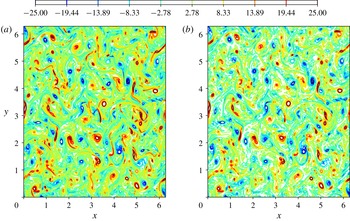
) are then obtained (the reader is directed to Maulik et al. (Reference Maulik, San, Rasheed and Vedula2019) for details related to the calculation of these quantities). Figure 1 visually quantifies the effect of the spectral domain filtering where the FDNS of a snapshot of vorticity is shown. We then introduce the a priori eddy viscosity given by
 $$\begin{eqnarray}\unicode[STIX]{x1D708}_{e}^{a}={\displaystyle \frac{\unicode[STIX]{x1D6F1}}{\unicode[STIX]{x1D6FB}^{2}\bar{\unicode[STIX]{x1D714}}}},\end{eqnarray}$$
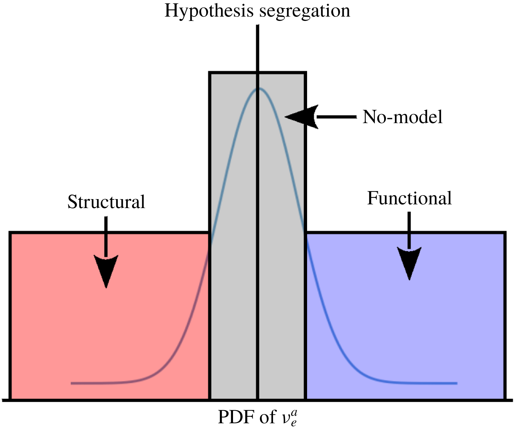
where all the terms on the right-hand side of the above equation are available through calculation from the DNS snapshots. The a priori eddy viscosity is centred at a value of zero (corresponding to a region where closure modelling is unnecessary) and has tails in the negative and positive directions. A core component of the hypothesis in this work stems from the fact that structural hypotheses are not limited to positive eddy-viscosity predictions alone. The reader may note that models utilizing the functional hypothesis always lead to positive eddy viscosities. The a priori eddy viscosities calculated from the DNS data are then projected onto a Gaussian distribution where values lying within a distance of 1 % of the standard deviation from the mean (of zero) are labelled as those requiring no closure (due to the low strength of the a priori eddy viscosity). Values lying beyond this range are labelled as functional or structural, depending on whether they are positive or negative, respectively. This information is encoded in one-hot labelling for a classification deployment and a corresponding schematic for this hypothesis segregation is shown in figure 2. It is observed that a large portion of the available data lies within the first standard deviation of the mean eddy viscosity. This leads to the potential of turbulence modelling classification being considered from an outlier detection point of view. A factor which motivates the choice of the Gaussian distribution is the nature of the decaying Kraichnan turbulence. However, we note that machine learning algorithms are also capable of classifying data belonging to complex distributions and that this hypothesis segregation may be tuned for better accuracy. Also, the choice of the 1 % hyper-parameter is also motivated by observing a posteriori training accuracies where it is noticed that a relatively simple architecture (mentioned next) is efficiently able to discern the varying hypothesis. Values greater than 1 % for model delineation led to reduced learning accuracies indicating that a physical delineation potentially exists in this projection and categorization. Essentially, categorizing closure bins for values greater than 1 % leads to poorer training and validation classification accuracies during the machine learning phase. This could indicate that a clear distinction between modelling requirements is lost through this segregation. Further study for adding complexity to the hypothesis segregation is thus, a necessity.
Visualization of the effect of Fourier cutoff filtering with DNS at
 $N^{2}=2048^{2}$
(a) and corresponding FDNS at
 $N^{2}=256^{2}$
(b).

Each label for the a priori eddy viscosity is also associated with an input kernel of grid-resolved quantities. This kernel is given by a stencil of 9 inputs each of vorticity and streamfunction (for a total of 18 input variables). These 9 inputs of each field are given by a query of the field quantity at a point on the coarse grid, the 4 adjacent points in each dimension and the 4 diagonally adjacent points. Each sample of our training data thus consists of 18 inputs of vorticity and streamfunction and outputs given by one-hot labels for the choice of closure modelling strategy. In this article, we have leveraged the fact that the means of vorticity and streamfunction are both very close to zero and do not necessitate normalization. In addition, the non-dimensionalized formulation of the governing equations implies that our inputs are all dimensionless. However, we note that for practical deployments of any local-kernel-based machine learning queries, grid-resolved quantities must be normalized and non-dimensionalized.
Data segregation for one-hot labelling. The a priori eddy viscosities are projected onto a Gaussian distribution where data beyond 1.0 % of the standard deviation are labelled as requiring structural (if negative) or functional (if positive) modelling. The remaining data points are classified as no-model cases.

Mathematically, if our input vector
 $\boldsymbol{p}$
resides in a
 $P$
-dimensional space and our desired output
 $\boldsymbol{q}$
resides in a
 $Q$
-dimensional space, this framework establishes a map
 $\mathbb{M}$
as follows:
 $$\begin{eqnarray}\mathbb{M}:\{p_{1},p_{2},\ldots ,p_{P}\}\in \mathbb{R}^{P}\rightarrow \{q_{1},q_{2},\ldots ,q_{Q}\}\in \mathbb{R}^{Q}.\end{eqnarray}$$
Accordingly, the framework utilized in this article leads to the following relation:
 $$\begin{eqnarray}\mathbb{M}:\{\boldsymbol{p}\}\in \mathbb{R}^{18}\rightarrow \{P(\boldsymbol{q}|\boldsymbol{p})\}\in \mathbb{R}^{3},\end{eqnarray}$$
where our input and output spaces are given by
 $$\begin{eqnarray}\left.\begin{array}{@{}c@{}}\boldsymbol{p}_{i,j}=\{\bar{\unicode[STIX]{x1D714}}_{i,j},\bar{\unicode[STIX]{x1D714}}_{i,j+1},\bar{\unicode[STIX]{x1D714}}_{i,j-1},\ldots ,\bar{\unicode[STIX]{x1D714}}_{i-1,j-1},\bar{\unicode[STIX]{x1D713}}_{i,j},\bar{\unicode[STIX]{x1D713}}_{i,j+1},\bar{\unicode[STIX]{x1D713}}_{i,j-1},\ldots ,\bar{\unicode[STIX]{x1D713}}_{i-1,j-1}\},\\ \boldsymbol{q}_{i,j}=\{P(\unicode[STIX]{x1D6F1}_{i,j}^{k}|\boldsymbol{p}_{i,j})\},\end{array}\right\}\end{eqnarray}$$
where
 $i,j$
refer to the spatial indices on the coarse grid (i.e. the point of deployment) and
 $k$
refers to the choice of closure scenario (i.e. structural, functional or no closure). We note here that the choice of the local stencil for ANN query reflects the discretization of the governing equations (with second-order accurate stencils requiring a
 $\pm 1$
query) and the use of the trapezoidal filter in AD. Also, note that our choice of input space is given by raw variable queries rather than derivatives (or other such engineered terms). This is motivated by an aversion to specify bias towards any particular quantity that may otherwise by learned implicitly by the network. However, we note that the classification workflow may benefit significantly from the inclusion of a feature engineering step prior to optimization. This is a subject of ongoing investigation.
Our optimal map
 $\mathbb{M}$
is then trained by the following loss function
 $$\begin{eqnarray}E(\boldsymbol{w})=-\mathop{\sum }_{n=1}^{N}\mathop{\sum }_{k=1}^{K}\{t_{nk}\log (y_{nk})+(1-t_{nk})\log (1-y_{nk})\},\end{eqnarray}$$
where
 $\boldsymbol{w}$
are the tuneable weights and biases of the network,
 $N$
is the total number of samples and
 $K=3$
is the total number of closure scenarios. Here,
 $t_{nk}$
refers to the target (or true) label of class
 $k$
and sample
 $n$
and
 $y_{nk}$
refers to its corresponding prediction. Note that one-hot encoding ensures that
 $t_{nk}$
values are always binary (Bishop Reference Bishop2006). For reference, our architecture is trained using the open-source deep learning software Tensorflow and is optimized with the use of ADAM, a popular gradient-descent-based optimizer.
Our learning architecture is given by a 5 hidden-layer deep neural network with 40 neurons each for calculating the conditional probabilities of the three closure scenarios pointwise in space and time. The hidden-layer neurons employ a rectified-linear activation and the output layer gives us softmax probabilities for the three classes. The scenario with the highest conditional probability is then deployed for model classification i.e.
 $$\begin{eqnarray}\unicode[STIX]{x1D6F1}_{i,j}^{ML}=\unicode[STIX]{x1D6F1}_{i,j}^{k}\text{ s.t. }\text{argmax}_{k}P(\unicode[STIX]{x1D6F1}_{i,j}^{k}|\boldsymbol{p}_{i,j}),\end{eqnarray}$$
where
 $\unicode[STIX]{x1D6F1}_{i,j}^{ML}$
refers to the machine-learning-based turbulence model computation at a point. In the case of model blending, the conditional probabilities for closure scenarios are used to find a linear combination of the standard Smagorinsky and the AD closures. In other words,
 $$\begin{eqnarray}\unicode[STIX]{x1D6F1}_{i,j}^{ML}=P(\unicode[STIX]{x1D6F1}_{i,j}^{AD}|\boldsymbol{p}_{i,j})\unicode[STIX]{x1D6F1}_{i,j}^{AD}+P(\unicode[STIX]{x1D6F1}_{i,j}^{SM}|\boldsymbol{p}_{i,j})\unicode[STIX]{x1D6F1}_{i,j}^{SM},\end{eqnarray}$$
where
 $\unicode[STIX]{x1D6F1}_{i,j}^{AD}$
and
 $\unicode[STIX]{x1D6F1}_{i,j}^{SM}$
are AD and Smagorinsky predictions for the turbulence model at a point. We note that the same learning framework is deployed in these two conceptually different scenarios.
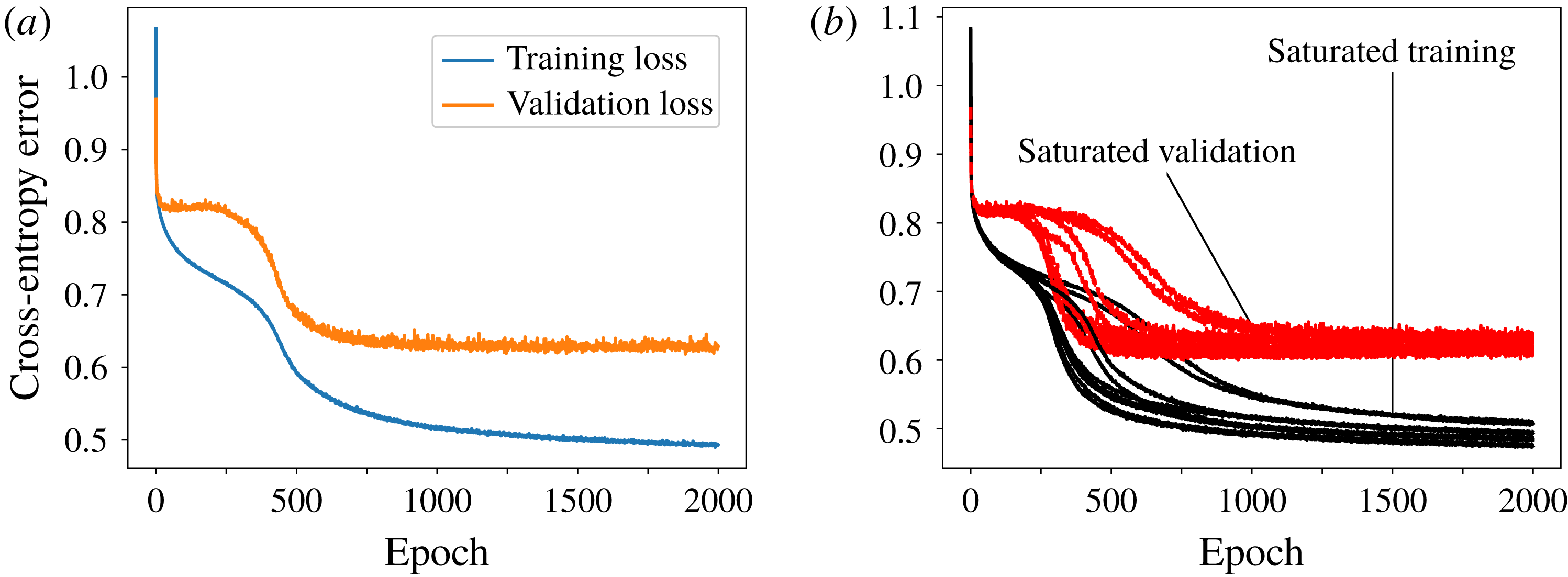
The framework is trained using the previously mentioned categorical cross-entropy error minimization for the one-hot encoded targets. A threefold cross-validation is utilized with a grid search for the number of layers (between 1 and 8) and number of neurons (between 10 and 100 at intervals of 10) to arrive at the optimal architecture mentioned previously. This optimal network is then trained for 2000 epochs to arrive at a classification accuracy of 79 % for training and approximately 68 % accuracy for validation. Convergence in validation loss was observed at around 1500 epochs as shown in figure 3. We note here that our validation data (amounting to one third of the total training data set) were not exposed to the network during gradient calculation in the back-propagation-based training procedure. Effectively, our learning is derived from two thirds of the total training data while our best model is chosen from that with the lowest validation loss. This is to ensure that the chances of network extrapolation are minimized. Multiple random initializations of our network weights led to similar training and validation behaviour as also seen in figure 3. Note one initialization is seen to take a longer time to converge as against the rest. The optimal learning is then deployed into a posteriori evolution of the Kraichnan turbulence test case where a pointwise closure deployment is performed for a variety of test cases. We also note that our labelled data are pre-processed to ensure that an equal number of samples are available from each classification regime to prevent our learning from prioritizing one outcome over the other two.
Neural network training and validation loss for the proposed learning framework for one random weight initialization showing convergence at around 1500 epochs (a). The training (in black) and validation (in red) saturation behaviour for different initializations also indicated convergence to similar accuracies as shown on the right. The best model was chosen according to lowest validation loss for reduced over-fitting in forward deployments.

4 Results
We proceed by examining the performance of our framework for various a posteriori deployments which act as a rigorous testing of our learning for both classification and blending. We remind the reader that a posteriori deployments of learning frameworks imply performance assessments in the presence of challenging numerical errors and represent the ultimate test of a data-driven framework. Briefly, the Kraichnan turbulence problem is specified by periodic boundary conditions on a rectangular domain and an initial condition which is given by an energy spectrum in wavenumber space. In this two-dimensional problem very fine scales are developed quickly and this leads to the classical
 $k^{-3}$
scaling of the kinetic-energy spectra which is a characteristic of the cascade of enstrophy in two-dimensional turbulence. The turbulence then decays gradually over time and thus represents an unsteady closure modelling assessment for our proposed framework.
We assess the viability of the proposed framework through energy spectrum calculations of various reduced-order deployments as well as vorticity structure functions obtained from the same. Time histories of the turbulent kinetic energy (denoted
 $TKE$
) and the variance of vorticity (denoted
 $\unicode[STIX]{x1D70E}^{2}(\bar{\unicode[STIX]{x1D714}})$
) are also plotted for forward deployments. Detailed explanations of the numerical schemes and energy spectrum calculations utilized for this problem may be found in Maulik & San (Reference Maulik and San2017c
). Briefly, all our spatial numerical schemes are second-order accurate and our time integration is third-order total-variation diminishing. Our vorticity structure function calculations are given by Grossmann & Mertens (Reference Grossmann and Mertens1992):
 $$\begin{eqnarray}S_{\unicode[STIX]{x1D714}}=\langle |\bar{\unicode[STIX]{x1D714}}(\boldsymbol{x}+\boldsymbol{r})-\bar{\unicode[STIX]{x1D714}}(\boldsymbol{x})|^{2}\rangle ,\end{eqnarray}$$
where the angle brackets indicate ensemble averaging and
 $\boldsymbol{x}$
indicates a position on the grid with
 $\boldsymbol{r}$
being a certain distance from this location. Our turbulent kinetic energy is given by
 $$\begin{eqnarray}TKE=\unicode[STIX]{x1D707}(u_{f}^{2}+v_{f}^{2}),\end{eqnarray}$$
where
 $u_{f}$
and
 $v_{f}$
are fluctuating quantities given by
 $$\begin{eqnarray}\displaystyle u_{f}=\bar{u}-\unicode[STIX]{x1D707}(\bar{u}), & & \displaystyle\end{eqnarray}$$
 $$\begin{eqnarray}\displaystyle v_{f}=\bar{v}-\unicode[STIX]{x1D707}(\bar{v}), & & \displaystyle\end{eqnarray}$$
and where
 $\unicode[STIX]{x1D707}(a)$
implies the spatial mean of a field variable
 $a$
. We note that the components of velocity
 $u,v$
are computed by second-order accurate central finite-difference implementations of
 $$\begin{eqnarray}\bar{u}={\displaystyle \frac{\unicode[STIX]{x2202}\bar{\unicode[STIX]{x1D713}}}{\unicode[STIX]{x2202}y}},\quad \bar{v}=-{\displaystyle \frac{\unicode[STIX]{x2202}\bar{\unicode[STIX]{x1D713}}}{\unicode[STIX]{x2202}x}}.\end{eqnarray}$$
In a similar manner the variance of vorticity, at each time step, is computed using
 $$\begin{eqnarray}\unicode[STIX]{x1D70E}^{2}(\bar{\unicode[STIX]{x1D714}})=\unicode[STIX]{x1D707}((\bar{\unicode[STIX]{x1D714}}-\unicode[STIX]{x1D707}(\bar{\unicode[STIX]{x1D714}}))^{2}).\end{eqnarray}$$
In all the following assessments, the proposed framework is denoted as ML (and specified to be deployed as a classifier or a blender) and it is compared to the AD and DS models. We remind the reader that the framework utilizes the static Smagorinsky model (denoted SM) with
 $C_{s}=1.0$
within its formulation but is assessed against the dynamic Smagorinsky (DS) approach. The reader may note that the value of
 $C_{s}=1.0$
proves over-dissipative for this particular test case as shown in Maulik et al. (Reference Maulik, San, Rasheed and Vedula2019). A test-filter ratio of two is utilized in our DS simulations along with the selection of a standard trapezoidal filter (San Reference San2014). We also note that the static Smagorinsky model with a prior information about
 $C_{s}=0.18$
yields qualitatively similar results to those obtained by the DS model in this particular test case (i.e. only the DS results are provided in our analysis and we refer to Maulik et al. (Reference Maulik, San, Rasheed and Vedula2018) for assessments with various
 $C_{s}$
values). Besides, once we consider the cost and ease of use criteria (Pope Reference Pope2004), probably the static Smagorinsky model with appropriately selected model coefficient (e.g.
 $C_{s}\approx 0.18$
) would be a better option in this particular test case due to its negligibly small overhead to the computational cost, however it provides a simplified test bed to assess the performance of our classification framework systematically when there is no a priori information on model parameters.
4.1 Model classification
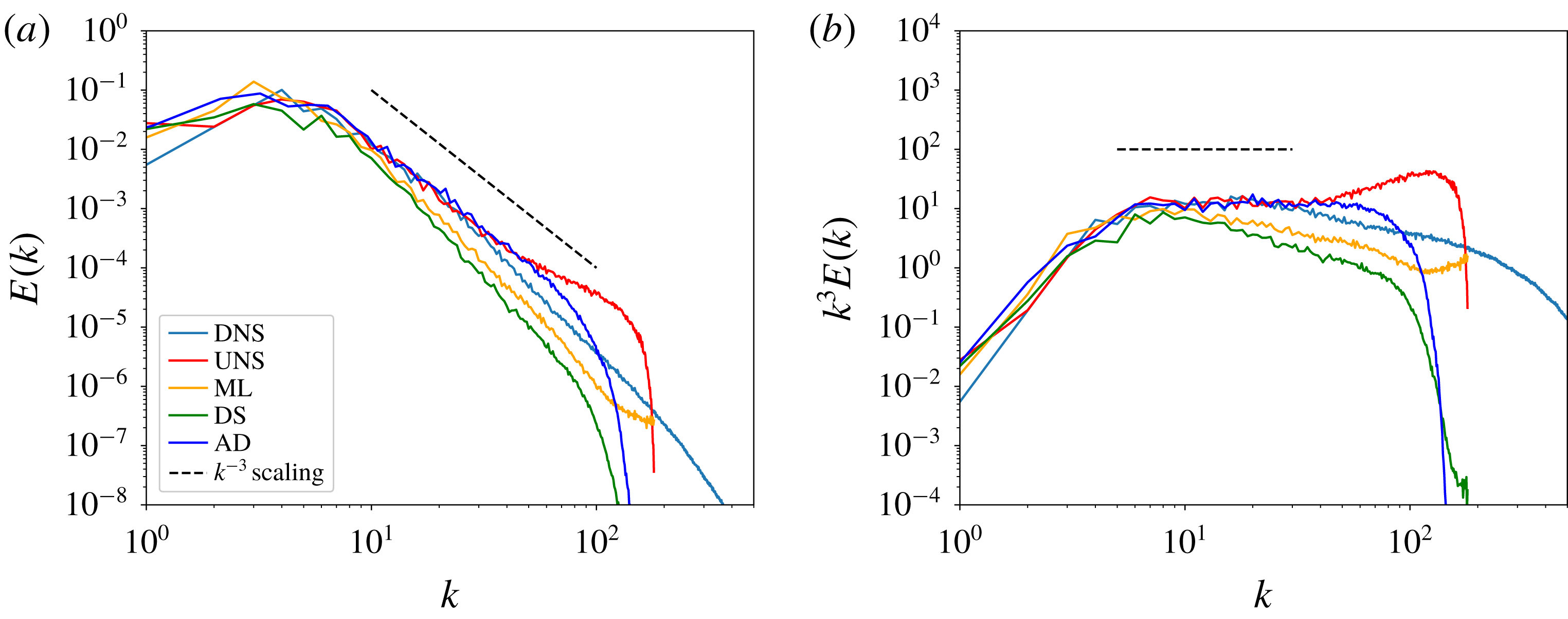
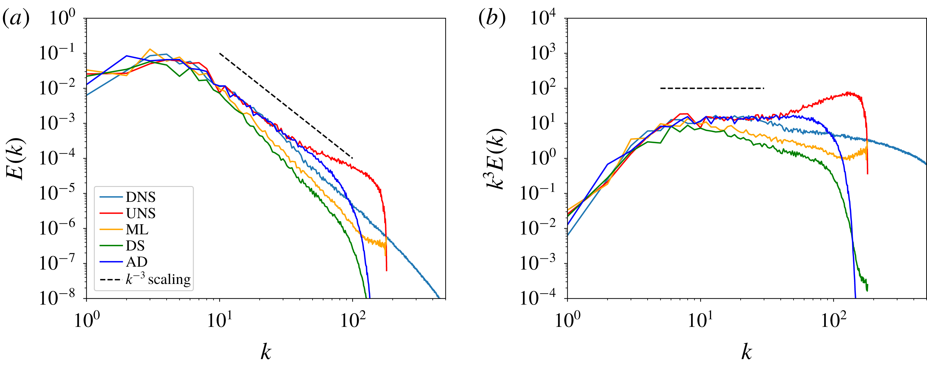
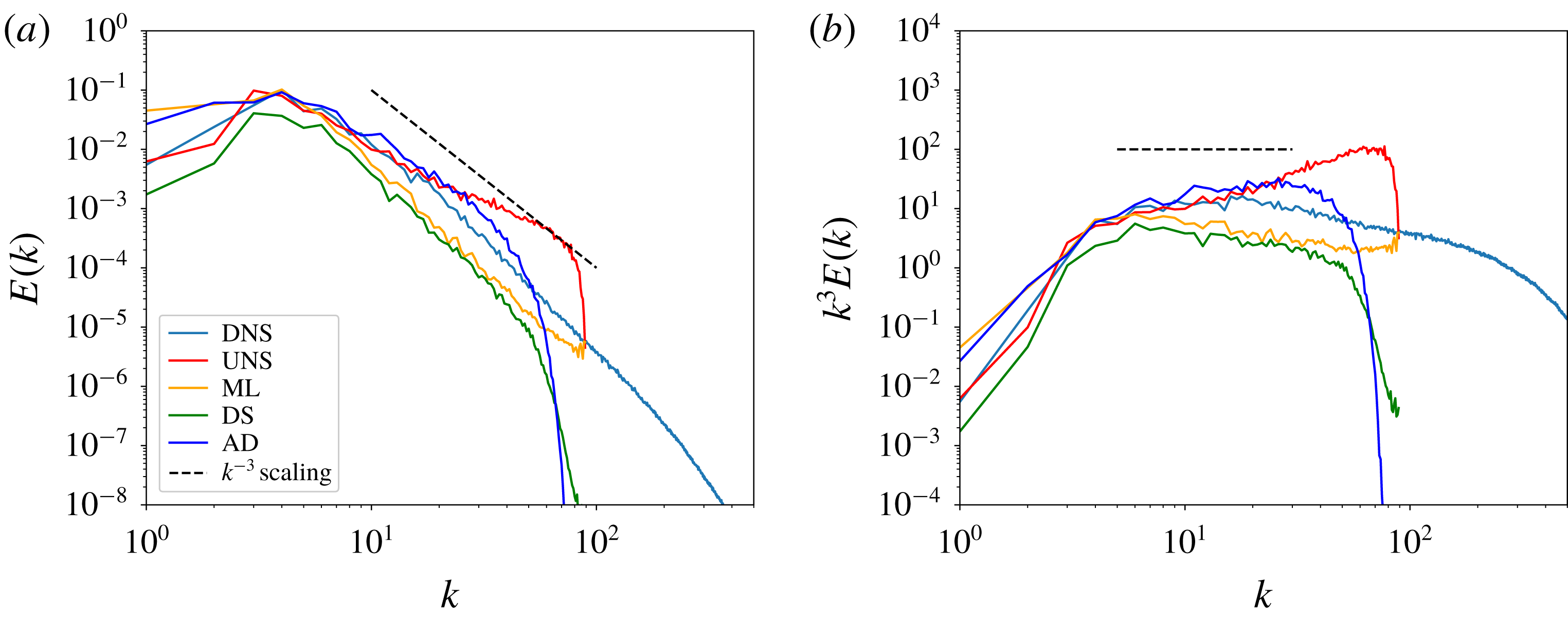
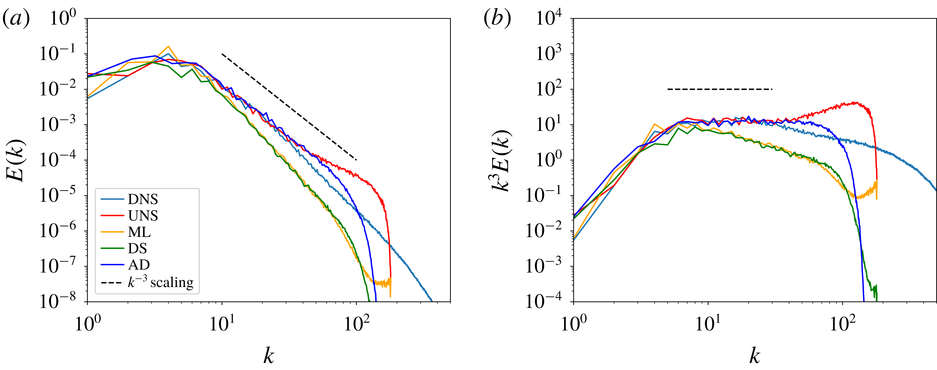
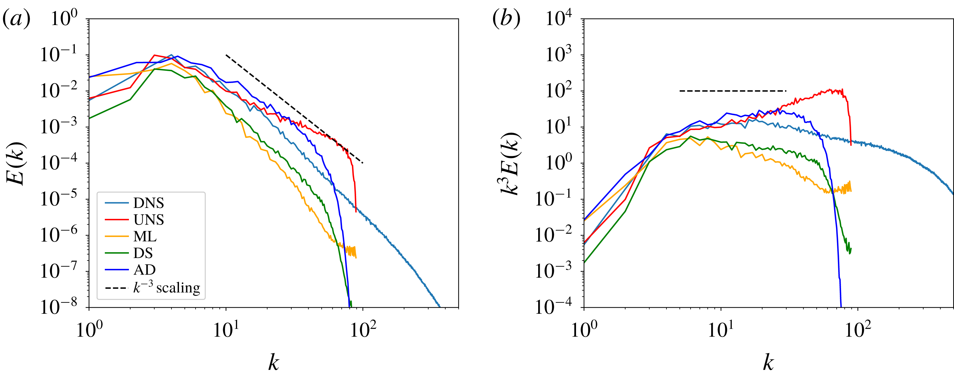
In this section, we deploy our learning framework as a classifier which spatio-temporally switches between three closure modelling hypotheses during flow evolution. Figure 4 shows the performance of our proposed framework for the forward deployment of the Kraichnan turbulence problem in the form of energy spectrum predictions at
 $t=4$
. For comparison, no-model results (denoted UNS), the DS method and AD are also shown along with DNS spectra. One can observe that the classifier balances the dissipative natures of the SM and AD hypothesis to obtain a performance similar to the that of the DS approach. While at the lower wavenumbers, the AD procedure seems to be more accurate in statistical capture, the higher wavenumbers are stabilized adequately by the classifier. We would like to note that the SM hypothesis with
 $C_{s}=1.0$
is highly dissipative and the classifier avoids its deployment to a large degree for improved a posteriori performance. We clarify that for spectral cutoff filtering, FDNS spectra and DNS spectra are identical till the grid cutoff wavenumber (Maulik et al.
Reference Maulik, San, Rasheed and Vedula2018).
A posteriori kinetic-energy spectra (a) and compensated kinetic-energy spectra (b) for
 $Re=32\,000$
at
 $t=4$
and at
 $N^{2}=256^{2}$
degrees of freedom. The proposed framework (deployed as a classifier) balances the dissipative natures of the AD and the DS models.

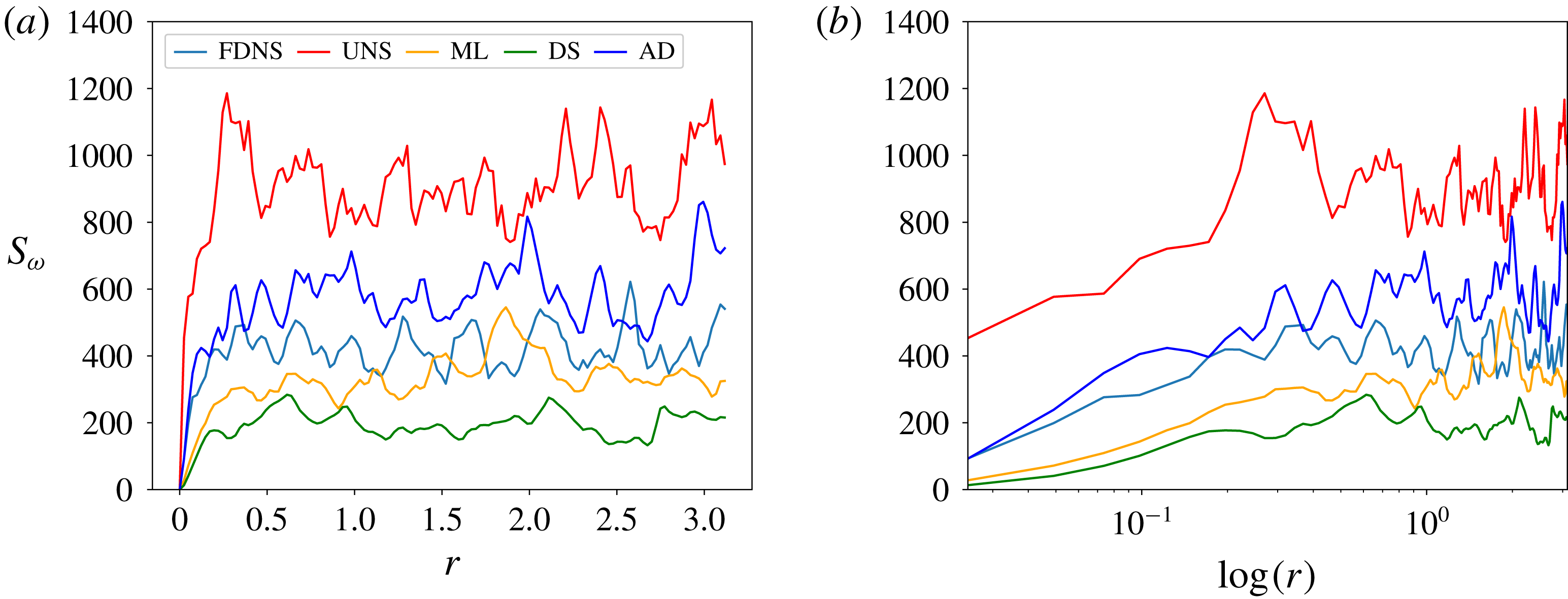
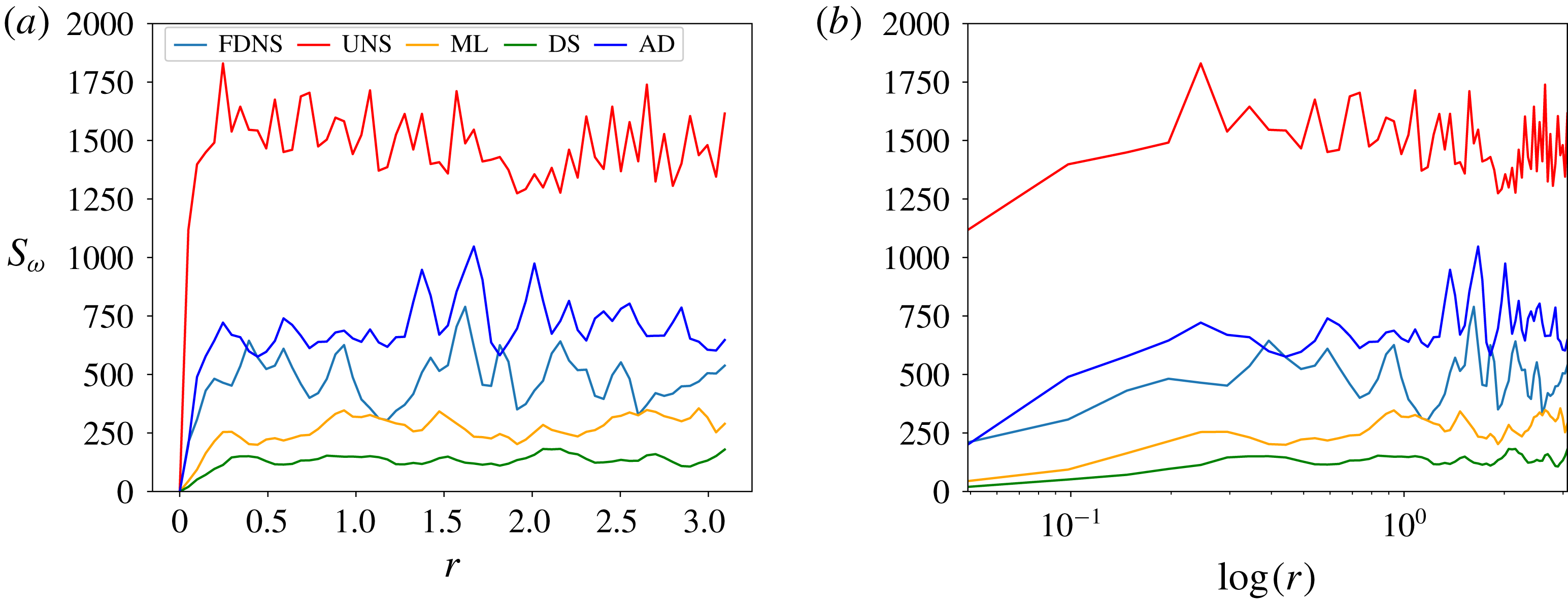
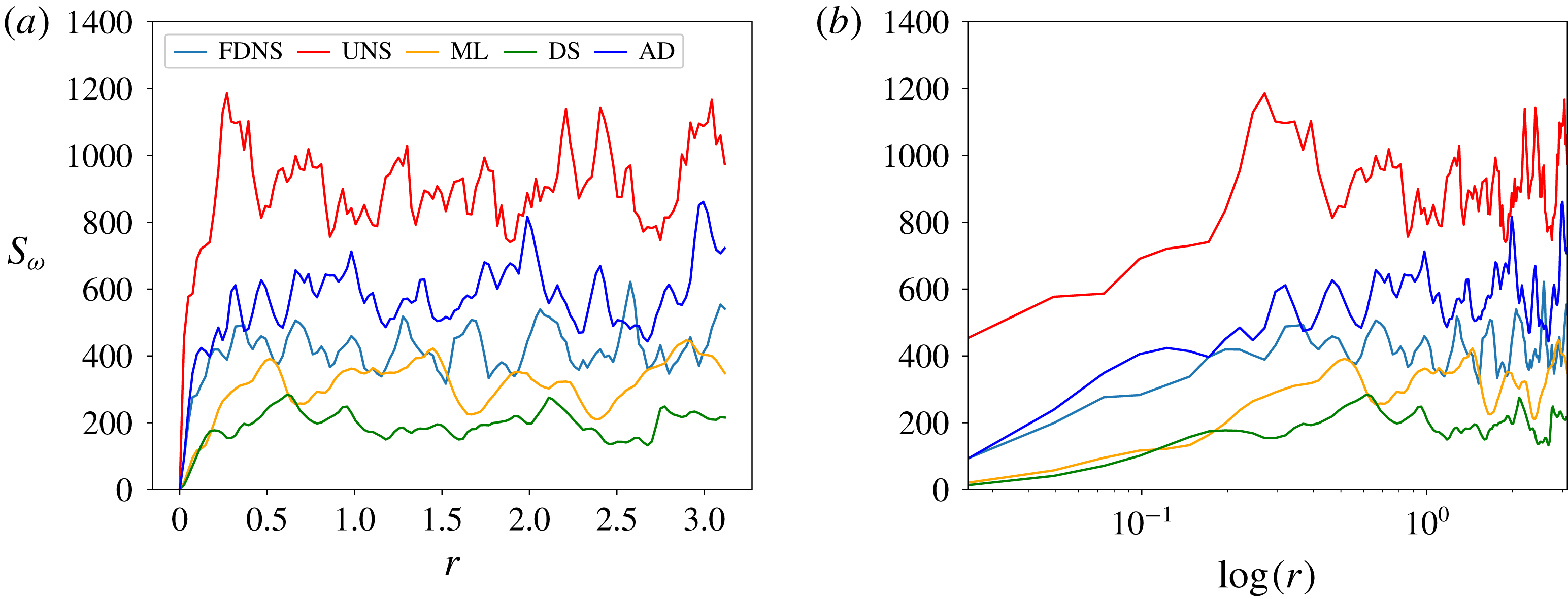
A posteriori vorticity structure functions plotted against
 $\boldsymbol{r}$
(a) and
 $\log (\boldsymbol{r})$
(b) for
 $Re=32\,000$
at
 $t=4$
and at
 $N^{2}=256^{2}$
degrees of freedom. It is observed that AD performs better in the near region whereas the proposed framework behaves similar to the DS approach.

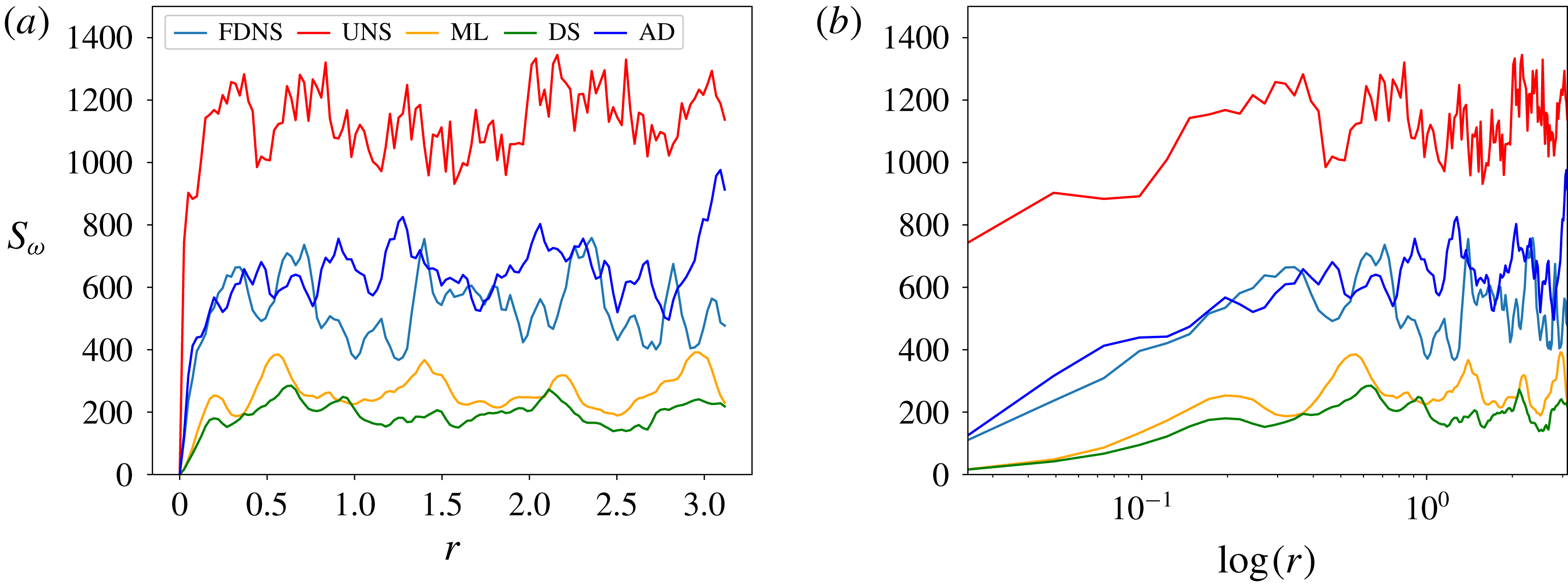
Figure 5 details vorticity structure function assessments in our domain where assessments with FDNS show that the proposed framework is adequately capable of stabilizing turbulence correlations at
 $t=4$
. We note that the structure functions are predicted more accurately by AD at low values of
 $\boldsymbol{r}$
whereas the proposed classifier behaves similar to a DS implementation, thereby indicating a dynamic dissipation on the grid. It may be due to the adaptive dissipation prioritizes noise removal and thus introduces errors at low values of
 $\boldsymbol{r}$
as seen through stable structure functions at saturation (i.e. at higher values of
 $\boldsymbol{r}$
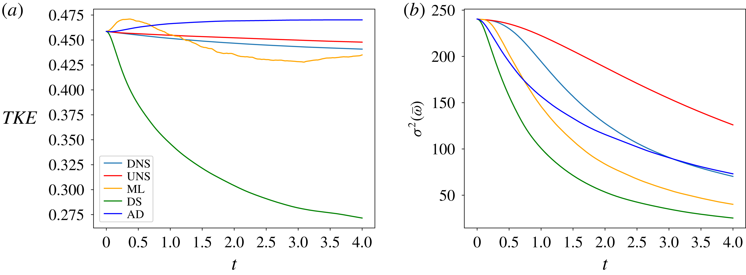
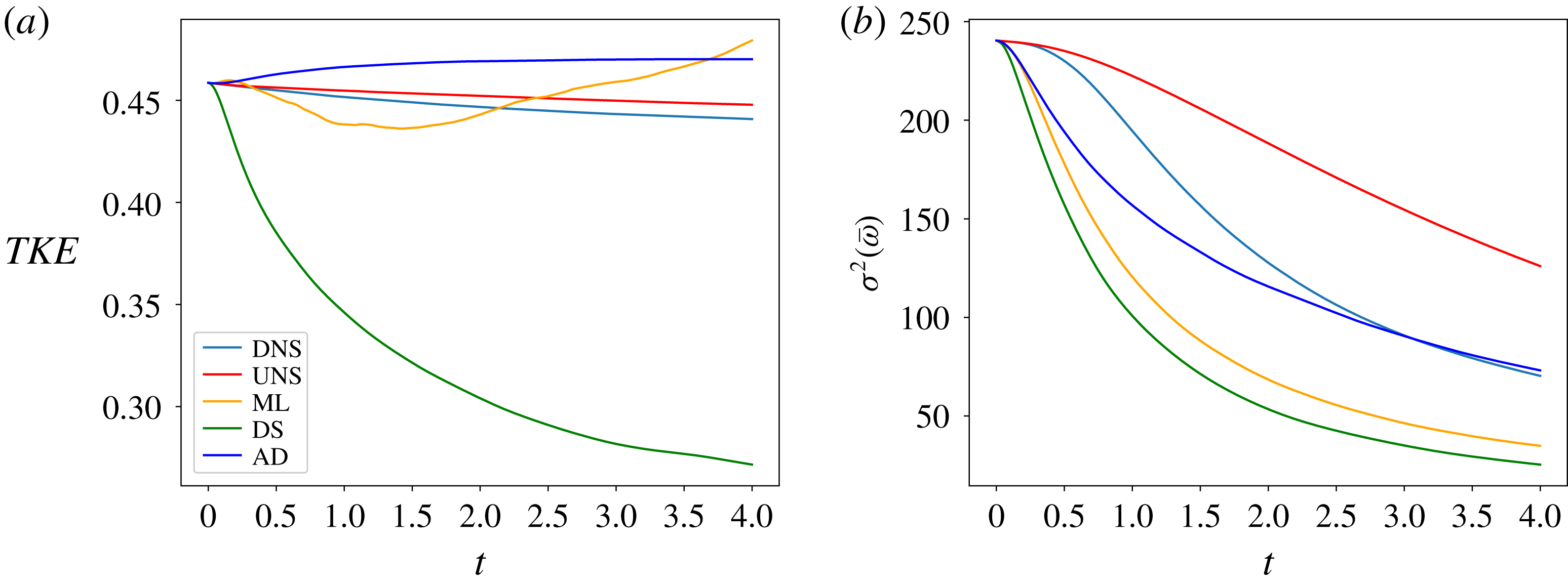
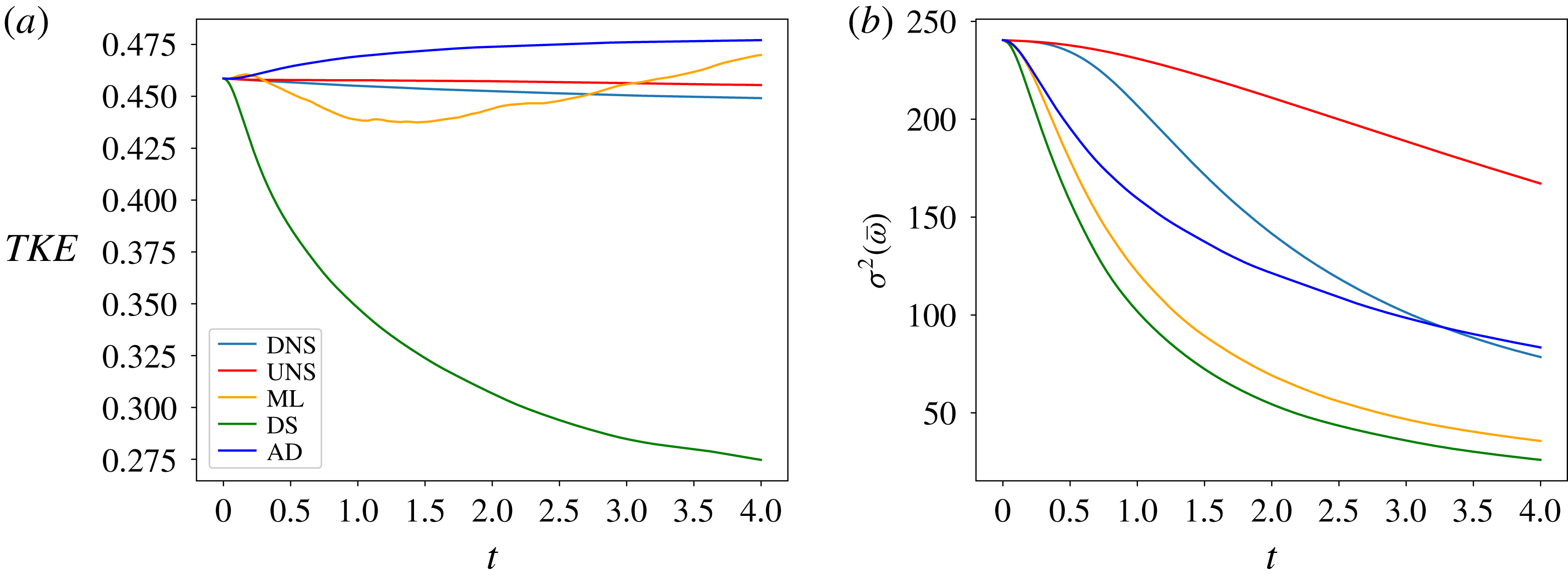
). A further assessment is deployed in the form of time histories of
 $TKE$
and
 $\unicode[STIX]{x1D70E}^{2}(\bar{\unicode[STIX]{x1D714}})$
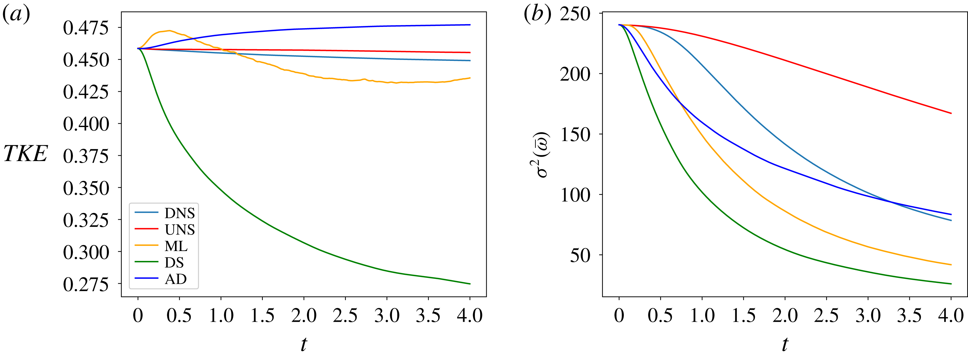
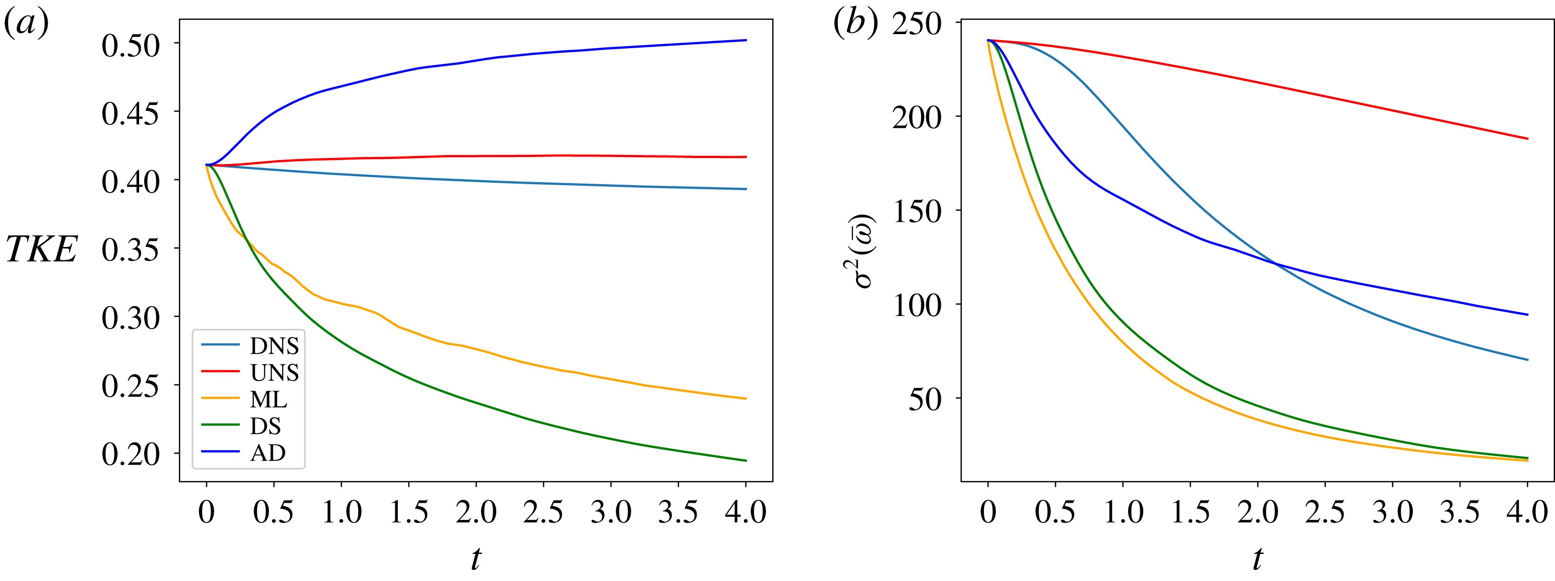
as shown in figure 6. Once again, the classifier is seen to have a varying trend in
 $TKE$
predictions compared to the AD and DS techniques indicating varying dissipation strengths. The vorticity variance predictions are also seen to be balanced between that of the DS and AD models indicating the balance of dissipative tendencies.
Time histories for turbulent kinetic energy (a) and vorticity variance (b) for
 $Re=32\,000$
at
 $N^{2}=256^{2}$
degrees of freedom. The proposed method can be seen to adapt between the behaviour of the AD and DS techniques.

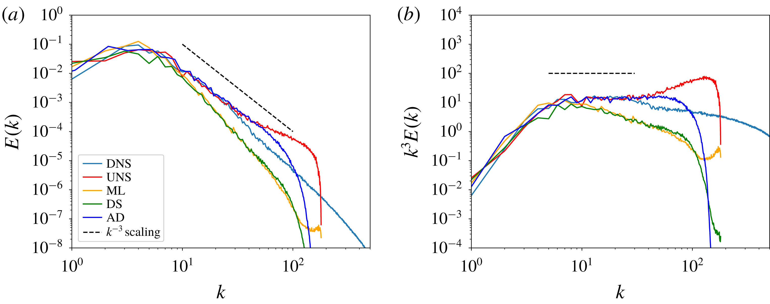
A posteriori kinetic-energy spectra (a) and compensated kinetic-energy spectra (b) for
 $Re=64\,000$
at
 $t=4$
and at
 $N^{2}=256^{2}$
degrees of freedom. This assessment displays closure effectiveness for a Reynolds number not utilized in the training data.

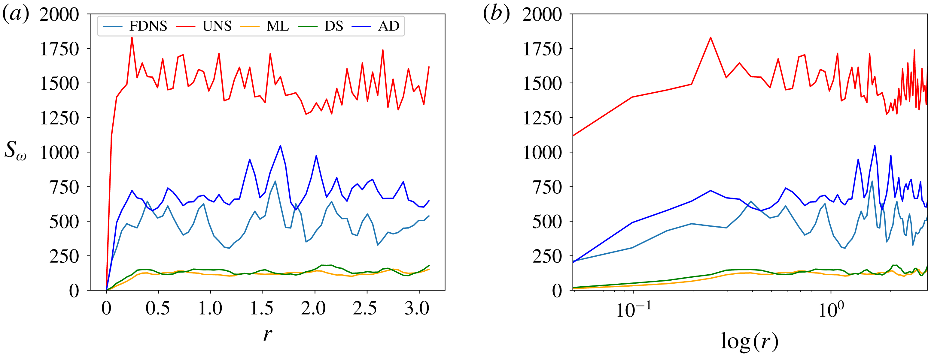
A posteriori vorticity structure functions plotted against
 $\boldsymbol{r}$
(a) and
 $\log (\boldsymbol{r})$
(b) for
 $Re=64\,000$
at
 $t=4$
and at
 $N^{2}=256^{2}$
degrees of freedom. It is observed that solely AD performs better in the near region whereas the proposed framework behaves similarly to the DS approach. The behaviour is similar to that observed for within training data regime deployment.

We proceed by performing a thorough validation of our learning framework by assessing its performance for prediction tasks that it has not been exposed to in training. This is established by testing closure efficiency for a Reynolds number of 64 000. We remind the reader that map optimization was performed solely for
 $Re=32\,000$
and this represents an additional validation of the learning. Kinetic energy spectra for this experiment are shown in figure 7 where it is observed that the classifier performs in a very similar fashion to the
 $Re=32\,000$
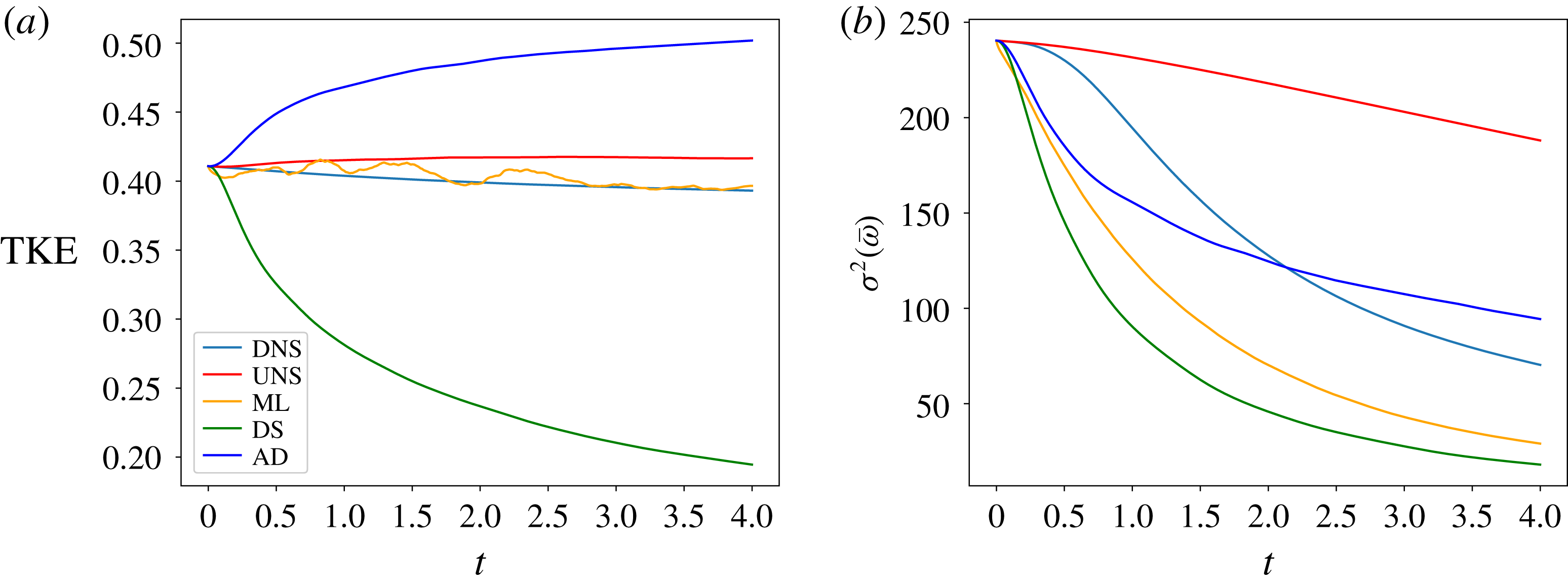
test case with AD performing more efficiently at the lower wavenumbers of the inertial range but the ML approach stabilizing high-wavenumber noise effectively. This indicates that the learning has generalized, at least on the current degree of coarse graining. We also perform additional assessments such as those shown in figure 8 and figure 9. The former shows the vorticity structure function trends for this out-of-training range learning assessment and the latter shows the time histories of
 $TKE$
and
 $\unicode[STIX]{x1D70E}^{2}(\bar{\unicode[STIX]{x1D714}})$
. Very similar behaviour for both these assessments is obtained when compared to the
 $Re=32\,000$
test case with time variation in trends seen in
 $TKE$
and vorticity variance. It can be clearly seen from figure 9 that the proposed ML approach does not yield monotonically decreasing
 $TKE$
for the present decaying turbulence problem and additional physical constraints might be incorporated either in training or deployment phases, a topic we would like to investigate further in our future studies.
Time histories for turbulent kinetic energy (a) and vorticity variance (b) for
 $Re=64\,000$
at
 $N^{2}=256^{2}$
degrees of freedom. The proposed method can be seen to adapt between the behaviour of the AD and DS techniques and acts as an additional validation for deployment to different Reynolds numbers.

A posteriori kinetic-energy spectra (a) and compensated kinetic-energy spectra (b) for
 $Re=32\,000$
at
 $t=4$
and at
 $N^{2}=128^{2}$
degrees of freedom. This assessment displays closure effectiveness for a coarse-grained resolution not utilized in the training data.

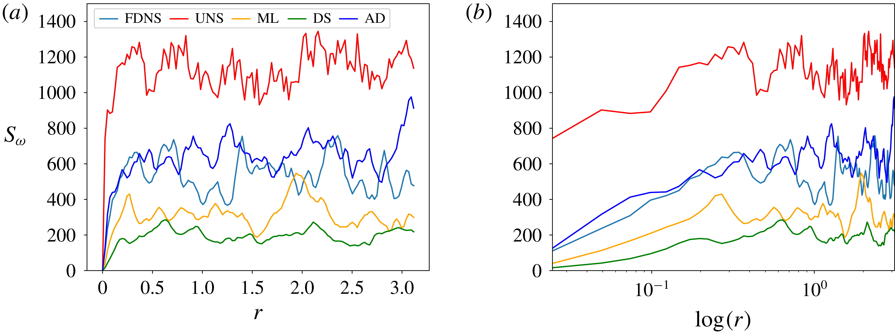
A posteriori vorticity structure functions plotted against
 $\boldsymbol{r}$
(a) and
 $\log (\boldsymbol{r})$
(b) for
 $Re=32\,000$
at
 $t=4$
and at
 $N^{2}=128^{2}$
degrees of freedom. It is observed that solely AD performs better in the near region whereas the proposed framework behaves similar to the DS approach. The behaviour is similar to that observed for within training resolution deployment.

The aforementioned test cases validated the learning of the classifier on different control parameters (and flow evolutions) given by the Reynolds number. We proceed by assessing the performance and stability of the classifier on a reduced degrees-of-freedom evolution given by
 $N^{2}=128^{2}$
. This test was to examine if the classifier could retain a viable learning for deployment on slightly different grid support. Figure 10 shows the kinetic-energy spectra for a deployment at this reduced degrees of freedom at a Reynolds number of 32 000. It is observed that the proposed classifier is able to avoid inaccuracies related to AD’s lack of dissipation. Indeed, it is well known that AD requires a sufficiently fine resolution in comparison to the eddy-viscosity hypothesis-based models for appropriate utilization of the underlying iterative inverse filtering (Guermond, Oden & Prudhomme Reference Guermond, Oden and Prudhomme2004; Germano Reference Germano2015). A similar trend may also be observed in figure 11 with the vorticity structure functions where once again the AD technique proves accurate at lower distances in comparison the DS and the ML methods. The ML classifier however is slightly more accurate than the DS approach. The time histories for
 $TKE$
and vorticity variance, shown in figure 12, display a greater amount of variation in the classification framework with
 $TKE$
values oscillating but remaining close to the DNS results. It must be noted that the no-model and AD hypotheses prevent the classifier from going into a fully SM deployment which is highly dissipative. This explains the similarity with DS results in terms of spectra and vorticity variance.
Time histories for turbulent kinetic energy (a) and vorticity variance (b) for
 $Re=32\,000$
at
 $N^{2}=128^{2}$
degrees of freedom. The proposed method can be seen to adapt between the behaviour of the AD and DS techniques and acts as an additional validation for deployment to similar coarse-grained resolutions.

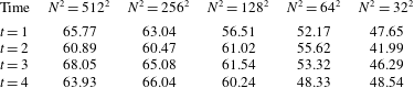
In addition to the test case with a slightly reduced grid resolution, we also perform a thorough grid-dependence check on the accuracy of our classification framework as shown in table 1. We perform a hypothesis segregation (as introduced previously) to label all points on a coarse grid with an optimal closure hypothesis and assess if the learning at
 $N^{2}=256^{2}$
is able to categorize them appropriately. It can be seen that accuracies around the same resolution as that of the training data are approximately similar to validation accuracy during network optimization. However, on intense coarse graining, accuracies are seen to drop significantly. However, we note that even at the coarsest resolution of
 $N^{2}=32^{2}$
, accuracies greater than 33 % indicate some form of learning retention.
Classification accuracy percentages for different grid resolutions a priori to illustrate how accurately our base learning can predict correct labels. Accuracies are seen to drop when resolutions are coarsened radically. However, some learning is retained as evidenced by accuracies greater than 33 %.

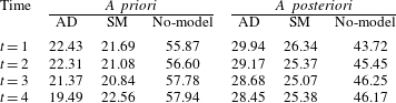
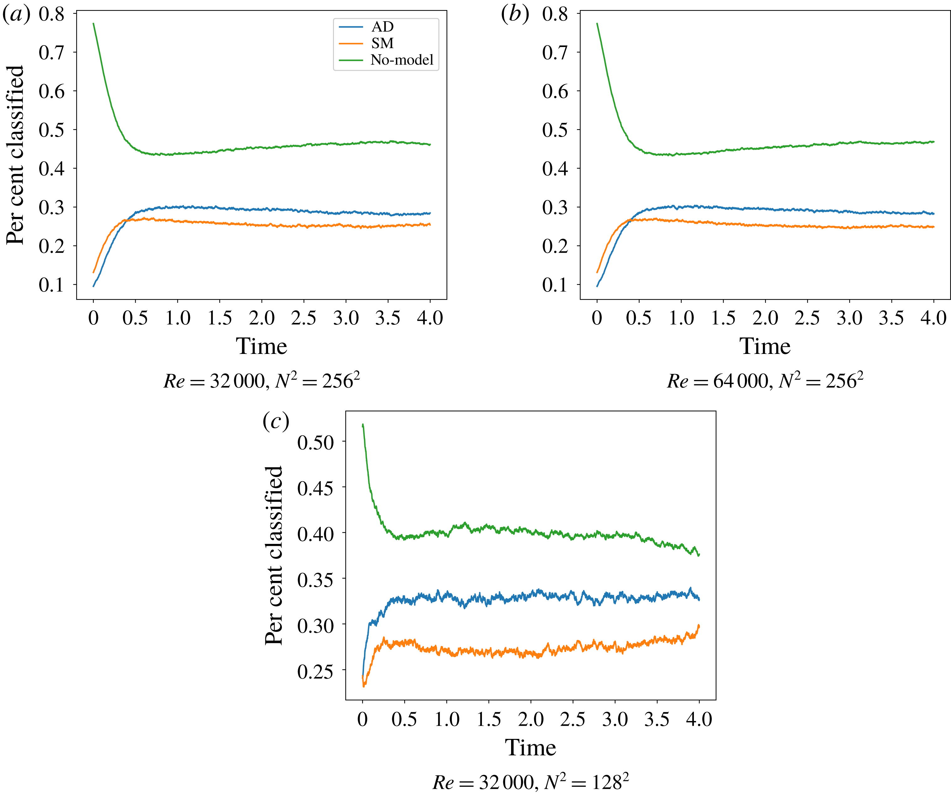
We also determine the effect of network deployment in the presence of numerical errors as shown in table 2 where it can be seen that a significant difference in hypothesis choices is observed. In particular, the a posteriori deployment of the classifier is seen to utilize a greater proportion of the turbulence closure hypotheses, in comparison to the no-model ones. This may be considered as proof of the classifier detecting greater stabilization requirements due to numerical error build-up. It is observed that the AD approach shows a greater increase in deployment than SM. This may be to offset the rather large inaccuracies of the lower wavenumbers in the exceptionally dissipative SM approach. Understanding the nature of classifier adaptation in the presence of numerical errors is an interesting subject of future research that may aid in improved decision making frameworks. We complement the data in table 2 by outlining the classification percentages of different hypotheses plotted against time for our three a posteriori deployments in figure 13. One may notice that the deployment of the framework at the coarser resolution of
 $N^{2}=128^{2}$
requires a higher degree of SM and AD classifications for successful stabilization. All experiments are seen to show a gradual increase in closure requirement as scale separation grows until they reach a level of saturation that is aligned with the slow turbulence decay.
Classification percentages in a priori and a posteriori. One can see deviation from trends due to numerical error accumulation (and greater utilization of closure classifications for subsequent stabilization). We note that an
 $N^{2}=256^{2}$
is utilized for this assessment.

The a posteriori classification percentages of the various modelling hypotheses for our three forward deployments. In all deployments it is observed that the utilization of AD and SM increases as the scale separation grows and saturates for the slow decay. Noticeably, the deployment at
 $N^{2}=128^{2}$
necessitates a higher proportion of AD and SM classifications for improved stabilization.

As a final qualitative analysis of our classifier, we plot a posterior contours from forward deployments at
 $N^{2}=256^{2}$
and
 $Re=32\,000$
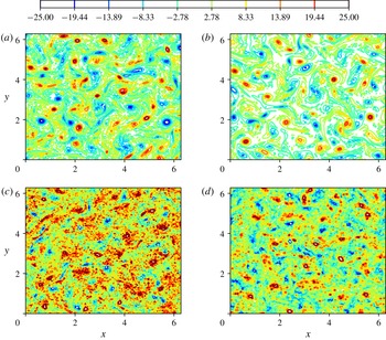
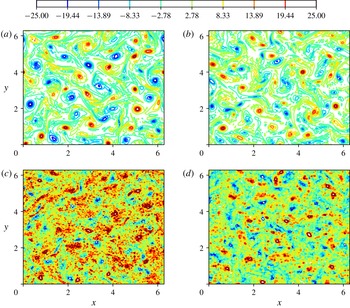
. In figure 14, vorticity contours from the ML, DS, AD and UNS simulations are shown to assess the stabilization effect of the different frameworks. The classifier can be seen to stabilize high-wavenumber noise adequately, in a manner similar to DS as previous statistics have reflected. The AD approach may be observed to be contaminated with noise that may potentially be harmful for long-time integration.
A posteriori contour results for
 $Re=32\,000$
at
 $N^{2}=256^{2}$
with the proposed classification framework shown (a), DS shown (b), UNS shown (c) and AD shown (d). These may be compared against FDNS contours qualitatively (in figure 1).

4.2 Model blending
In this section, we deploy our learning in a different manner by utilizing the outputs (i.e. the conditional probabilities of each hypothesis) as a pre-multiplier of the prediction of each modelling hypothesis. We utilize this formulation instead of the direct prediction of sub-grid contribution coefficients by observing that a greater degree of stability is imparted to the flow evolution. Indeed, direct regression with sub-grid quantities has been seen to require a posteriori post-processing for stability (Maulik et al. Reference Maulik, San, Rasheed and Vedula2018, Reference Maulik, San, Rasheed and Vedula2019) due to energy accumulation in the coarse-grained super-grid (when negative eddy viscosities are predicted effectively). We note that the various clipping approaches are common in LES practices (Sagaut Reference Sagaut2006) to avoid numerical instabilities. Indeed, within ML-based regression studies, one can simply use a rectified-linear activation function for the output layer (i.e. clipping negative values) when predicting data-driven eddy-viscosity distribution from an ANN architecture. In our classification framework, we recognize (as a limitation), that the utilization of a conditional-probability outputs to linearly combine turbulence modelling predictions from different hypotheses digresses from the core idea of a categorical cross-entropy error minimization. While the loss function used for training our map predicts conditional probabilities for each turbulence closure scenario, we interpret these probabilities as coefficients for the three closure models to set up a projection basis for the final value of the closure. However, as results shall show, the proposed method acts as an effective instrument for blending models in a posteriori without the requirement of any truncation for numerical stability. We would also like to emphasize here that the same learning is applicable for both classification and blending. We perform a similar set of assessments as outlined in § 4.1.
Figure 15 shows the performance of the blending formulation for a Reynolds number of 32 000 and at
 $t=4$
with
 $N^{2}=256^{2}$
degrees of freedom with kinetic-energy spectra. It is observed that the proposed procedure recovers a dissipative behaviour that is very similar to the DS approach. This is due to balancing the coefficients of the AD and SM predictions which adapt to the dynamic dissipation requirement of the flow. Overall, it is observed that the framework behaves in a similar manner to the classifier presented previously with dissipation preventing the accumulation of high-wavenumber errors but causing a mismatch in the inertial range spectrum capture. However, the dissipation is dynamic and it prevents the overwhelming damping of the SM deployment by balancing with the AD predictions adaptively. This is reflected in figure 16 as well where the vorticity structure functions once again show that the AD method is more accurate at lower values of
 $\boldsymbol{r}$
but the blending allows for a prediction akin to the DS technique. Figure 17 shows the time histories of the
 $TKE$
and the
 $\unicode[STIX]{x1D70E}^{2}(\bar{\unicode[STIX]{x1D714}})$
for the proposed framework compared to DS, AD and UNS. The vorticity variance shows a trend close to the DS approach as expected but the
 $TKE$
trends are once again not uniform.
A posteriori kinetic-energy spectra (a) and compensated kinetic-energy spectra (b) for
 $Re=32\,000$
at
 $t=4$
and at
 $N^{2}=256^{2}$
degrees of freedom. The proposed framework (deployed as a model blending mechanism) behaves similar to the DS approach at the inertial wavenumbers. We remind the reader that the blending is dynamic between AD and SM.

A posteriori vorticity structure functions plotted against
 $\boldsymbol{r}$
(a) and
 $\log (\boldsymbol{r})$
(b) for
 $Re=32\,000$
at
 $t=4$
and at
 $N^{2}=256^{2}$
degrees of freedom. It is observed that solely AD performs better in the near region whereas the proposed blending (once again) behaves similar to the DS approach. We remind the reader that the blending is dynamic between AD and SM.

Time histories for turbulent kinetic energy (a) and vorticity variance (b) for
 $Re=32\,000$
at
 $N^{2}=256^{2}$
degrees of freedom. The proposed blending technique shows a varying
 $TKE$
capture behaviour due to its adaptive dissipation. Note that the blending is dynamic between AD and SM.

In a fashion similar to that employed in § 4.1, we deploy assessments of the blending method to out-of-training predictions for validation. We start with an a posteriori deployment at
 $Re=64\,000$
and
 $N^{2}=256^{2}$
degrees of freedom and observe that the learning is sufficiently generalizable. This is observed from figure 18 where kinetic-energy spectra show an aligned prediction to the previous test case. Vorticity structure functions and time histories, shown in figures 19 and 20 respectively, illustrate a similar behaviour to that observed for
 $Re=32\,000$
. This implies that the learning, whether utilized as a classifier or a blending mechanism, is generalizable. We also deploy the blending framework at a different degree of freedom (
 $N^{2}=128^{2}$
) to assess it is stable to a slightly different grid support and trends similar to the classifier are observed wherein the framework focuses on dissipation to stabilize the higher wavenumbers in contrast with AD. This is observed in figure 21 for kinetic-energy spectra and figure 22 for the vorticity structure functions. Figure 23 shows time-series quantities for this test case with both
 $TKE$
and vorticity-variance trends resembling the DS method closely. This also echoes with the performance of the classifier where a coarser grid resolution led to a performance that was observed to be biased towards the eddy-viscosity hypothesis. However, further studies are necessary to quantify how the model orients itself to compensate for loss of grid resolution or anisotropies in the flow configuration in a posteriori deployment.
A posteriori kinetic-energy spectra (a) and compensated kinetic-energy spectra (b) for
 $Re=64\,000$
at
 $t=4$
and at
 $N^{2}=256^{2}$
degrees of freedom. The proposed framework (deployed as a model blending mechanism) behaves similar to the DS approach at the inertial wavenumbers. Note that the blending is dynamic between AD and SM and training is performed using
 $Re=32\,000$
data alone.

A posteriori vorticity structure functions plotted against
 $\boldsymbol{r}$
(a) and
 $\log (\boldsymbol{r})$
(b) for
 $Re=64\,000$
at
 $t=4$
and at
 $N^{2}=256^{2}$
degrees of freedom. It is observed that solely AD performs better in the near region whereas the proposed blending (once again) behaves similar to the DS approach. We remind the reader that the blending is dynamic between AD and SM and training is performed using
 $Re=32\,000$
data alone.

Time histories for turbulent kinetic energy (a) and vorticity variance (b) for
 $Re=64\,000$
at
 $N^{2}=256^{2}$
degrees of freedom. We remind the reader that the blending is dynamic between AD and SM and training is performed using
 $Re=32\,000$
data alone.

A posteriori kinetic-energy spectra (a) and compensated kinetic-energy spectra (b) for
 $Re=32\,000$
at
 $t=4$
and at
 $N^{2}=128^{2}$
degrees of freedom. The proposed framework (deployed as a model blending mechanism) behaves similar to the DS approach at the inertial wavenumbers. We remind the reader that the blending is dynamic between AD and SM and training is performed using
 $Re=32\,000$
and
 $N^{2}=256^{2}$
data alone.

A posteriori vorticity structure functions plotted against
 $\boldsymbol{r}$
(a) and
 $\log (\boldsymbol{r})$
(b) for
 $Re=32\,000$
at
 $t=4$
and at
 $N^{2}=128^{2}$
degrees of freedom. It is observed that solely AD performs better in the near region whereas the proposed blending (once again) behaves similar to the DS approach. We remind the reader that the blending is dynamic between AD and SM and training is performed using
 $Re=32\,000$
and
 $N^{2}=256^{2}$
data alone.

Time histories for turbulent kinetic energy (a) and vorticity variance (b) for
 $Re=32\,000$
at
 $N^{2}=128^{2}$
degrees of freedom. The proposed blending technique behaves more dissipatively due to the reduced grid support. We remind the reader that the blending is dynamic between AD and SM and training is performed using
 $Re=32\,000$
and
 $N^{2}=256^{2}$
data alone.

To conclude this section we show qualitative results from the vorticity contours at the final time of the numerical experiments for our proposed framework and their benchmark counterparts in figure 24. This examination gives us an intuition of the stabilization effect of the proposed framework and it is seen that the predictions are very closely aligned with the DS results. We note that the blending calculation of closure models may be considered an extension of traditional techniques which directly couple structural methods (such as AD) and eddy-viscosity-based techniques (such as dynamic Smagorinsky) (Habisreutinger et al. Reference Habisreutinger, Bouffanais, Leriche and Deville2007).
A posteriori contour results for
 $Re=32\,000$
at
 $N^{2}=256^{2}$
with the proposed blending framework shown (a), DS shown (b), UNS shown (c) and AD shown (d). These may be compared against FDNS contours qualitatively (in figure 1).

5 Conclusions and significance
In this article we have proposed a novel data-driven strategy to dynamically assess the utility of a turbulence modelling hypothesis in an LES framework. This strategy is built on the hypothesis that DNS data may be utilized to assess areas where structural or functional models may be more appropriate in an LES deployment. Our hypothesis segregation and subsequent training culminates in a learning that may deployed as a classifier of turbulence models at each point on the LES grid as well as a blending technique for balancing turbulence models with different dissipative strengths. When deployed as a classifier, our proposed framework may also predict a ‘no-model’ situation wherein no sub-grid source-term is deployed. When deployed as a blending mechanism, the learning linearly combines the AD and static Smagorinsky hypothesis premultiplied by their respective conditional probabilities to obtain another hybrid dissipation mechanism. Both frameworks utilize the same learning and are assessed through similar experiments a posteriori. Furthermore, a similar architecture can be constructed to provide hybrid intelligent implicit LES approaches by toggling between non-dissipative and dissipative numerical schemes, a topic we intend to investigate further in a future study.
We have rigorously assessed the deployment of our machine learning strategy through the utilization of a Kraichnan turbulence test case. Our assessments are made for Reynolds number values both within and outside that utilized in training to ensure that a generalizable turbulence closure has been developed. In addition, we have also assessed if the proposed closure can be deployed on a coarser grid than one it was trained for. The dissipative and scale-content capture of the proposed framework is compared to the AD and DS techniques through the use of kinetic-energy spectra, vorticity structure functions and time histories of
 $TKE$
and vorticity variance showing a dynamic dissipation akin to the DS. In particular, the statistical fidelity of the data-driven frameworks is seen to be inferior to the AD technique, which provides better estimates of the kinetic-energy spectra at lower wavenumbers and also provides most accurate estimates of the vorticity structure function. However, the focus on high-wavenumber noise attenuation leads to no grid cutoff error accumulation and the statistical results of the ML models are very similar to DS in all assessments. Also, it is observed that the data-driven closure (whether deployed as a classifier or a blending instrument) adequately captures the
 $k^{-3}$
scaling expected for the kinetic-energy spectra for the Kraichnan turbulence case and attempts to strike an optimal balance between the dissipative functional kernel and the noise-prone structural kernel. This behaviour is interesting as the model classifies solely between AD and the static Smagorinsky hypothesis indicating the extreme dissipation of the latter at
 $C_{s}=1.0$
is effectively alleviated by the spatio-temporal blending. Our closure, thus, attempts to blend the strengths of both modelling strategies to overcome their individual weaknesses while attempting to preserve trends from DNS.
In terms of future opportunities for this idea, the data-driven element of closure identification lends to the potential development of closures that may discern the physical characteristics of different flow scenarios. However, some challenges associated with progress in this research include considerations of invariance properties, which we have identified as a next step. In order to generalize adequately, Galilean invariance must be built in to the data-driven closure described in this study. This is a limitation of the current approach which does not explicitly enforce these considerations. For instance, research is underway to investigate the response of this system to invariant inputs of localized stencils (rather than raw field variables) to ensure that predictions are invariant as well. We may also look at augmenting our input data set through the use of transformations which make the classifier resistant to extrapolation (Ling et al. Reference Ling, Jones and Templeton2016a ). We note that the model blending idea proposed here can be devised to ensure invariance properties by choosing a suitable projection basis (Ling et al. Reference Ling, Kurzawski and Templeton2016b ). Our frameworks may then be assessed for transformed validation data. We expect an optimal formulation that relies on invariant inputs to map to a basis of invariant outputs for predicting an appropriate closure as a culmination of this study. The effect of input spaces (invariant or otherwise) on generalizability and accuracy must also be studied. This is an extension to the current formulation which takes a rudimentary approach of exposing the framework to all available grid-resolved information in the local stencil. Another major limitation of our study is the finite number of assessments in decaying two-dimensional turbulence where the vortex stretching mechanism is absent.
While the computational costs of the proposed framework have not been studied in detail, an efficient deployment of the proposed framework would need graphical processing unit integration of any practical CFD simulation. The latter would lead to efficient learning queries since all the spatial domain information would be available to the common memory. Overall, without performing any additional effort by optimizing our deployment code, the proposed ML approach adds computational overhead that is approximately 2.5 times greater than that of required for simulating the problem with the DS model due to arithmetic computations within 5 hidden-layer network architecture at each time step. In practice, the trade-off between the training accuracy (hence the number of layers and the number of neurons at each layer) and computational efficiency of the ML-based models should be carefully analysed. A priori hyper-parameter search might yield a deep network architecture for an accurate training representation, but it might provide a costly deployment model for forward simulations. This would suggest to perform feature selection and simplify network architecture as recommended by Wang et al. (Reference Wang, Luo, Li, Tan and Fan2018). Another future direction identified in this research is the exposure of different two-dimensional turbulence physics to the classification framework to identify if closure choices can also be influenced by the training data regime. Success in that regard would allow for ‘train and forget’ closures in problems that have unsteady physics that span fundamentally different turbulence modelling requirements.
Acknowledgements
This material is based upon work supported by the US Department of Energy, Office of Science, Office of Advanced Scientific Computing Research under Award Number DE-SC0019290. O.S. gratefully acknowledges their support. We also acknowledge the support of NVIDIA Corporation for our research and the assistance of Jesse Schafer, Oklahoma State University High Performance Computing Center, for technical support.
Disclaimer. This report was prepared as an account of work sponsored by an agency of the United States Government. Neither the United States Government nor any agency thereof, nor any of their employees, makes any warranty, express or implied, or assumes any legal liability or responsibility for the accuracy, completeness, or usefulness of any information, apparatus, product, or process disclosed, or represents that its use would not infringe privately owned rights. Reference herein to any specific commercial product, process, or service by trade name, trademark, manufacturer, or otherwise does not necessarily constitute or imply its endorsement, recommendation, or favoring by the United States Government or any agency thereof. The views and opinions of authors expressed herein do not necessarily state or reflect those of the United States Government or any agency thereof.