


1. Introduction
Landscape heterogeneities are intrinsically linked to locally elevated surface fluxes of momentum, heat, humidity and other quantities, including pollen and dust. Such surface fluxes are a product of land–atmosphere interactions affecting the hydrologic cycle, whereas local heterogeneities create microclimates that profoundly alter the existence of idealised (equilibrium) atmospheric surface layer (ASL) conditions.
Horizontally homogeneous neutrally stratified ABL (Wyngaard Reference Wyngaard2010) flow over a homogeneous distribution of roughness elements is composed of a roughness sublayer and an inertial layer aloft, where the former is occupied by vortical mixing processes regulated by the spatial extent of roughness elements (Raupach, Antonia & Rajagopalan Reference Raupach, Antonia and Rajagopalan1991; Raupach, Finnigan & Brunet Reference Raupach, Finnigan and Brunet1996; Jimenez Reference Jimenez2004; Castro Reference Castro2007; Ghisalberti Reference Ghisalberti2009), whereas the latter is occupied by wall-attached eddies (Townsend Reference Townsend1976) and large-scale motions (Hutchins & Marusic Reference Hutchins and Marusic2007). For a homogeneous distribution of elements with aggregate height,  $h$, the roughness sublayer depth,
 $\lambda _\mathcal {R} \approx 5 h$ (Grass Reference Grass1971; Raupach et al. Reference Raupach, Antonia and Rajagopalan1991; Harmon & Finnigan Reference Harmon and Finnigan2007). In practice, however, roughness elements are seldom distributed homogeneously across landscapes, but exhibit local heterogeneity that confounds prognostic descriptions based upon horizontally homogeneous conditions (Bou-Zeid et al. Reference Bou-Zeid, Anderson, Katul and Mahrt2020; Stoll et al. Reference Stoll, Gibbs, Salesky, Anderson and Calaf2020).
Such spatial heterogeneity is realised via distributions of, for example, buildings, topographic undulations, sand dunes, wind turbines or vegetation. For this study, we have specifically focused on spatial heterogeneity realised via distributions of virtual trees within large-eddy simulation (LES) of ASL turbulence; it is stressed, though, that virtual trees serve a more general purpose in behaving as generalised drag elements (Belcher, Jerram & Hunt Reference Belcher, Jerram and Hunt2003).
Flow over vegetation has been studied for many years (Finnigan Reference Finnigan2000), where preceding studies have focused on aggregate canopy dynamics (Shaw & Schumann Reference Shaw and Schumann1992; Raupach et al. Reference Raupach, Finnigan and Brunet1996; Su et al. Reference Su, Shaw, Paw, Moeng and Sullivan1998), the coupled effect of canopies and topography (Belcher, Harman & Finnigan Reference Belcher, Harman and Finnigan2012), turbulence response to the multiscale nature of trees (Graham & Meneveau Reference Graham and Meneveau2012; Bai, Katz & Meneveau Reference Bai, Katz and Meneveau2015), flow response with variable canopy layout (Bailey & Stoll Reference Bailey and Stoll2013) and fundamental vortical flow processes above canopies (Finnigan, Shaw & Patton Reference Finnigan, Shaw and Patton2009; Bailey et al. Reference Bailey, Stoll, Pardyjak and Mahaffee2014; Bailey & Stoll Reference Bailey and Stoll2016). Though by no means exhaustive, this literature survey points to the depth of prior contributions in this area. Bailey & Stoll (Reference Bailey and Stoll2013) specifically addressed the problem of ASL flow aloft sparse canopy arrangements, although in their case sparsity was realised via streamwise heterogeneity. In this work, we are specifically interested in spanwise heterogeneity and the non-trivial confluence of effects associated with variation in the streamwise and spanwise spacing between adjacent elements.
1.1. Roughness-driven secondary flows
In recent years, substantial new work has demonstrated the passive actuator-like influence of spanwise heterogeneity in surface texture on wall turbulence. This largely originates with Hinze (Reference Hinze1967), who reported results of spanwise-variable surface roughness in rectangular duct flows. Hinze showed that such an arrangement induced Reynolds-averaged secondary flows, which differed from contemporaneous observations of secondary ‘corner’ flows (Prandtl Reference Prandtl1952; Hoagland Reference Hoagland1960; Brundrett & Baines Reference Brundrett and Baines1964; Perkins Reference Perkins1970; Gessner Reference Gessner1973). These studies were foremost in establishing the role of Reynolds (turbulent) stress spatial heterogeneity in sustenance of secondary flows or turbulent secondary flow of the second kind (Bradshaw Reference Bradshaw2003). This can be appreciated via the Reynolds-averaged vorticity transport equation:
 \begin{equation} \dfrac{\mathrm{D} \langle {\boldsymbol \omega} \rangle_t}{\mathrm{D} t} = \langle {\boldsymbol \omega} \rangle_t \boldsymbol{\cdot} \boldsymbol{\nabla} \langle {\boldsymbol u} \rangle_t + Re_\tau^{{-}1} \nabla^2 \langle {\boldsymbol \omega} \rangle_t - \boldsymbol{\nabla} \times \left( \boldsymbol{\nabla} \boldsymbol{\cdot} \langle {\boldsymbol u}^\prime \otimes {\boldsymbol u}^\prime \rangle_t \right), \end{equation}
where  $\langle \,\boldsymbol {\cdot}\, \rangle _t$ denotes time averaging of an ergodic system,
 ${\boldsymbol \omega } = \boldsymbol {\nabla } \times {\boldsymbol u}$ is vorticity and
 ${\boldsymbol u}$ is velocity, the first, second and third terms on the right-hand side denote the stretching-and-tilting term, dissipation and turbulent torque. Here
 $Re_\tau = u_* \delta / \nu$ is a bulk Reynolds number, where
 $u_*$ is the shear velocity,
 $\delta$ is the flow (ASL) depth,
 $\nu$ is kinematic viscosity and
 $\langle {\boldsymbol u}^\prime \otimes {\boldsymbol u}^\prime \rangle _t$ is the Reynolds-averaged Reynolds (turbulent) stress tensor. Note that in this article, the first, second and third component of any vector denote magnitude in the streamwise (
 $x$), spanwise (
 $y$) and vertical direction (
 $z$), respectively; velocity and vorticity vectors have components,
 $\{ u, v, w \}$ and
 $\{ \omega _x, \omega _y, \omega _z \}$, respectively; averaging of sample quantity,
 $\theta ({\boldsymbol x})$, over dimension,
 $a$, is denoted by
 $\langle \theta ({\boldsymbol x}) \rangle _a$.
Prior work has determined that the spatial heterogeneity of the Reynolds stresses, so-called ‘turbulent torque’ or Prandtl's secondary flow of the second kind, can sustain Reynolds-averaged secondary flows in a variety of scenarios. From flows in square ducts (Bradshaw Reference Bradshaw2003, and references therein), to hydraulic flows responding to spanwise-variable gravel roughness or aquatic canopy depth (Wang & Cheng Reference Wang and Cheng2005; Vermaas, Uijttewaal & Hoitink Reference Vermaas, Uijttewaal and Hoitink2011), to idealised channel flows over canonical spanwise-heterogeneous roughness (Anderson et al. Reference Anderson, Barros, Christensen and Awasthi2015a). Other studies have reported similar results in turbulent boundary layer flows over complex roughness s(Barros & Christensen Reference Barros and Christensen2014; Pathikonda & Christensen Reference Pathikonda and Christensen2017), spanwise-heterogeneous ‘herringbone’ roughness (Nugroho, Hutchins & Monty Reference Nugroho, Hutchins and Monty2013; Kevin et al. Reference Kevin, Monty, Bai, Pathikonda, Nugroho, Barros, Christensen and Hutchins2017), spanwise-heterogeneous roughness derived via ‘LEGO’ arrangements (Vanderwel & Ganapathisubramani Reference Vanderwel and Ganapathisubramani2015; Medjnoun, Vanderwel & Ganapathisubramani Reference Medjnoun, Vanderwel and Ganapathisubramani2018, Reference Medjnoun, Vanderwel and Ganapathisubramani2020) and other canonical arrangements (Stroh et al. Reference Stroh, Schäfer, Frohnapfel and Forooghi2020).
Within this work, a longstanding issue has been consistent assignment of secondary flow polarity with respect to the topographic elements. Consider, for now, the streamwise component of (1.1) for the case of high- $Re_\tau$ channel flow (i.e. absent streamwise heterogeneity):
 \begin{equation} \langle v \rangle_t \dfrac{\partial \langle {\omega}_x \rangle_t}{\partial y} + \langle w \rangle_t \dfrac{\partial \langle {\omega}_x \rangle_t}{\partial z} = \dfrac{\partial^2 }{\partial z^2} \langle {v}^\prime {w}^\prime \rangle_t - \dfrac{\partial^2 }{\partial y^2} \langle {v}^\prime {w}^\prime \rangle_t + \dfrac{\partial^2}{\partial y \partial z} \left( \langle {v}^\prime {v}^\prime \rangle_t - \langle {w}^\prime {w}^\prime \rangle_t \right). \end{equation}
Some groups have found that the secondary flow polarity is such that  $\langle w \rangle _t < 0$ (downwelling) above relative peaks in roughness (Willingham et al. Reference Willingham, Anderson, Christensen and Barros2013; Barros & Christensen Reference Barros and Christensen2014; Anderson et al. Reference Anderson, Barros, Christensen and Awasthi2015a; Yang & Anderson Reference Yang and Anderson2017a; Awasthi & Anderson Reference Awasthi and Anderson2018), while others have persistently found that
 $\langle w \rangle _t > 0$ (upwelling) above the elements (Goldstein & Tuan Reference Goldstein and Tuan1998; Vanderwel & Ganapathisubramani Reference Vanderwel and Ganapathisubramani2015; Medjnoun et al. Reference Medjnoun, Vanderwel and Ganapathisubramani2018, Reference Medjnoun, Vanderwel and Ganapathisubramani2020). In this article, LES has been used to address this apparent disagreement, where the aforementioned virtual trees are used to systematically isolate the arrangement ‘triggers’ needed to activate downwelling and upwelling above high roughness regions. Results will show that the confluence of streamwise and spanwise spacing confound automatic categorisation.
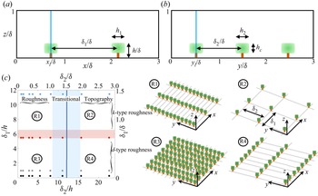
This can be appreciated from figure 1, which shows the canopy attributes assessed for this article, streamwise spacing between successive trees,  $\delta _1$, and spanwise spacing between adjacent rows,
 $\delta _2$, where panels (a) and (b) show canopy transects in the
 $x$–
 $z$ and
 $y$–
 $z$ plane, respectively. In addition, figure 1 shows the tree height,
 $h$, with all geometric arguments normalised by ASL thickness,
 $\delta$; additional tree attributes (
 $h_1$,
 $h_2$,
 $h_c$ and
 $d_t$) are common to all cases and quantitative values are provided in the subsequent text. There has been significant interest in the role of
 $\delta _2$. Yang & Anderson (Reference Yang and Anderson2017b) showed that the intensity, measured via circulation,
 ${\varGamma }$, of roughness-driven secondary flows scaled as
 ${\varGamma } \sim \delta _2^2$ for
 $\delta _2/\delta \lesssim 1$, and began declining for
 $\delta _2/\delta \gtrsim 1$. Medjnoun et al. (Reference Medjnoun, Vanderwel and Ganapathisubramani2018), also, hypothesised on a similar process with their ‘significance’ parameter. Yet, both antecedent studies report differing secondary flow direction relative to the high-roughness regions. Results presented herein show that streamwise spacing between elements,
 $\delta _1$, drives a reversal in the secondary flow direction. These arguments are summarised in figure 1(c)
 $\delta _1$–
 $\delta _2$ parameter space, where
 $\delta _2$ is placed on the abscissa. In this panel, for context, we have superimposed annotations for the roughness, transitional and topography regimes, where the top and bottom abscissa show
 $\delta _2$ normalised by flow depth and canopy height, respectively.
Schematic of tree canopy arrangements addressed as part of the research effort. Panels (a,b) show canopy visualisation in the streamwise–wall-normal and spanwise–wall-normal plane, respectively, where annotations are provided for streamwise spacing between subsequent trees,  $\delta _1/\delta$, spanwise spacing between rows of trees,
 $\delta _2/\delta$, canopy height,
 $h/\delta$, and the streamwise, spanwise and vertical extent of individual tree canopy,
 $h_1$,
 $h_2$ and
 $h_c$, respectively. Table 1 summarises specific cases; tree ‘trunks’ are modelled as square with side length,
 $d_t$. Panel (c) shows the
 $\delta _1$–
 $\delta _2$ parameter space (normalised by
 $h$ and
 $\delta$), with annotations superimposed for flow-roughness regimes predicated upon
 $\delta _1$ (
 $k$- or
 $d$-type roughness) (Jimenez Reference Jimenez2004) and
 $\delta _2$ (roughness, transitional and topography regimes) (Yang & Anderson Reference Yang and Anderson2017b). In panel (c), filled symbols indicate the location within
 $\delta _1$–
 $\delta _2$ parameter space corresponding to individual cases, where
 $d$-type cases, intermediate cases and
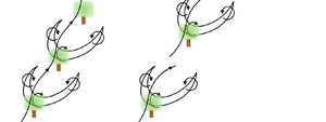
 $k$-type cases are denoted via filled black and grey circles, filled red circles and filled blue circles, respectively (see main text). Shown also are regimes R1, R2, R3 and R4, with accompanying sketches for each regime depicted on the right, for context.

The dynamical significance of  $\delta _2$ can be appreciated from prior work: for
 $\delta _2/\delta \lesssim 1.5$, the spanwise regions between adjacent rows is inadequate to enable coexisting
 $\delta$-scale secondary cells. In this case, secondary cells emanating from the roughness elements dominate, resulting in persistent upwelling above the elements. In contrast, for
 $\delta _2/\delta \gtrsim 1.5$, there exists sufficient spanwise spacing for two adjacent, roughness-driven,
 $\delta$-scale secondary flows to coexist. This has been graphically depicted in figure 1(c), where regions R1/R3 and R2/R4 correspond with ‘roughness’ and ‘topography’ arrangements, which are graphically illustrated on the right. These illustrative panels highlight the relatively small and larger spanwise spacing. However, prior work in this area has failed to consider dynamical implications of streamwise spacing between streamwise-aligned topographic elements,
 $\delta _1$, and yet this parameter is itself a significant roughness parameter (Jimenez Reference Jimenez2004; Flack, Schultz & Connelly Reference Flack, Schultz and Connelly2007; Flack & Schultz Reference Flack and Schultz2010; Yang et al. Reference Yang, Sadique, Mittal and Meneveau2016).
1.2.  $k$- and $d$-type roughness


Prior research has shown that the spatial distribution of roughness elements has major implications for instantaneous and Reynolds-averaged flow response. Here,  $\delta _1$ has been shown to regulate the flow response (Perry, Schofield & Joubert Reference Perry, Schofield and Joubert1969; Macdonald, Griffiths & Hall Reference Macdonald, Griffiths and Hall1998), where for
 $\delta _1/h \lesssim 5$ and
 $\delta _1/h \gtrsim 5$ the flow response is defined as d- and k-type, respectively (see also the reviews by Raupach et al. (Reference Raupach, Antonia and Rajagopalan1991), Jimenez (Reference Jimenez2004), Chung et al. (Reference Chung, Hutchins, Schultz and Flack2021) and references therein). The distinction between these roughness regimes is predicated upon flow response: for the
 $d$-type regime, canopy voids are occupied by
 $h$-scale vortices and the aloft flow ‘skims’ across the roughness (Macdonald et al. Reference Macdonald, Griffiths and Hall1998); for
 $k$-type regime, the relatively larger intra-canopy voids provide sufficient spatial extent for separation of
 $h$-scale vortices. Herein, it will be shown that longstanding concerns regarding direction of roughness-driven secondary flows can be attributed to
 $\delta _1/h$.
The confluence of  $\delta _1$ and
 $\delta _2$ can be further appreciated from figure 1(c), where
 $\delta _1$ is shown on the ordinate (normalised by
 $h$ and
 $\delta$ at left and right, respectively). The transition from
 $d$- to
 $k$-type, itself not a fixed quantity, is highlighted via the superimposed transparent red band at
 $\delta _1/h \approx 6$. With this, we see the emergence of regimes R1 to R4, based upon topography attributes within the
 $\delta _1$–
 $\delta _2$ parameter space. It is apparent that regimes R3 and R2 correspond with dense and sparse arrangements, respectively, whereas regimes R1 and R4 manifest as spanwise and streamwise ridges, respectively, where the former will induce internal boundary layer (IBL) formation (Antonia & Luxton Reference Antonia and Luxton1971; Bou-Zeid, Meneveau & Parlange Reference Bou-Zeid, Meneveau and Parlange2005) and the latter will sustain Reynolds-averaged counter-rotating secondary cells (Anderson et al. Reference Anderson, Barros, Christensen and Awasthi2015a).
It is self-evident that distinct response modalities, from IBL (regime R1) to streamwise secondary cells (regime R4), will collapse for case with  $\delta _1/h \approx 6$ and
 $\delta _2/\delta \approx 1.5$. In this study, topographic arrangements were designed precisely for the purpose of targeting these cases, as will be outlined in the following developments. Results will show that secondary flow polarity is consistent with prior work, but that
 $\delta _1/h$ regulates the
 $\delta _2$ threshold at which polarity is reversed.
1.3. This study
We have used LES to conduct an extensive parametric study on the influence of  $\delta _1$ and
 $\delta _2$ for roughness-driven secondary flows. Results will show that, as per prior studies, secondary flow intensity strengthens with increasing spanwise spacing,
 $\delta _2$. This is recorded via circulation in the spanwise–wall-normal plane, as per prior studies (Yang & Anderson Reference Yang and Anderson2017b; Anderson et al. Reference Anderson, Yang, Shrestha and Awasthi2018; Anderson Reference Anderson2019). Likewise, it will be shown that downwelling and upwelling occurs above the elements for distinct ‘topography’ and ‘roughness’ regime cases, irrespective of the
 $k$- or
 $d$-type configuration. We, however, show that the transition to downwelling, i.e. secondary flow polarity reversal, occurs first for the largest
 $\delta _1/h$.
Although virtual trees are used as drag elements, these can be interpreted as general wall-mounted obstacles, which play the role of absorbing momentum fluxes (i.e. conceptual scientific deductions realised from the work are not expected to differ if the work were repeated with, for example, cubes instead of virtual trees) (Ghisalberti Reference Ghisalberti2009). In § 2.1, details of the LES code and computational cases are presented. Results are presented in § 3, and concluding remarks are presented in § 4. In the Appendix, results of LES modelling of flow over canopies considered in a prior article are presented (Bailey & Stoll Reference Bailey and Stoll2013), to demonstrate efficacy of the present simulations.
2. Numerical methodology and cases
2.1. LES code
The spatially filtered incompressible momentum transport equation is solved,  $\mathrm {D}_t \tilde {\boldsymbol u}({\boldsymbol x},t) = {\boldsymbol f}({\boldsymbol x},t)$, where the grid-filtering operation is performed via convolution with the filtering kernel,
 $\tilde {\boldsymbol u}({\boldsymbol x},t) = G_{\varDelta } \star {\boldsymbol u}({\boldsymbol x},t)$, where
 $\widetilde {\ldots }$ denotes a grid-filtered quantity.
 ${\boldsymbol f} = - \rho ^{-1} \boldsymbol {\nabla } p - \boldsymbol {\nabla } \boldsymbol {\cdot} {\boldsymbol \tau } + {\boldsymbol e}_1 {\varPi } + {\boldsymbol f}_b$, where
 $\rho$ is density,
 $\boldsymbol {\nabla } p$ is a pressure correction required to preserve a divergence-free (incompressible) flow,
 $\boldsymbol {\nabla } \boldsymbol {\cdot} \tilde {\boldsymbol u} = 0$,
 ${\boldsymbol \tau } = \widetilde {{\boldsymbol u}^\prime \otimes {\boldsymbol u}^\prime }$ is the subgrid-scale stress tensor, where
 ${\boldsymbol u}^\prime = {\boldsymbol u} - \tilde {\boldsymbol u}$,
 ${\varPi } = \rho ^{-1}\,\mathrm {d} P_0 / \,\mathrm {d}\kern0.7pt x$ is an imposed pressure gradient and
 ${\boldsymbol f}_b$ is a body force used to represent the presence of virtual trees within the computational mesh (discussion to follow). Note that the shear-normalised viscous stress tensor,
 $Re_\tau ^{-1} \nabla ^2 \tilde {\boldsymbol u}$, is omitted because
 $Re_\tau = u_* \delta \nu ^{-1} \sim {O}(10^7)$ for the inertia-dominated (fully rough) flow conditions typical of geophysical/engineering wall-sheared turbulence, where
 $u_*$ is the shear velocity,
 $\delta$ is flow depth (channel half-height) and
 $\nu$ is kinematic viscosity. A solenoidal velocity field is maintained by computing the divergence of the momentum transport equation,
 $\mathrm {D}_t [ \boldsymbol {\nabla } \boldsymbol {\cdot} \tilde {\boldsymbol u}({\boldsymbol x},t) ] = \boldsymbol {\nabla } \boldsymbol {\cdot} {\boldsymbol f}({\boldsymbol x},t)$, applying the divergence-free condition,
 $\boldsymbol {\nabla } \boldsymbol {\cdot} \tilde {\boldsymbol u} = 0$ and solving the resultant pressure Poisson equation with Neumann conditions at the domain top and bottom,
 $\partial \tilde {p}/\partial z |_{z / \delta = 1} = 0$ and
 $\partial \tilde {p}/\partial z |_{z / \delta = 0} = 0$, respectively. Spectral discretisation is used in the horizontal directions, whereas vertical gradients are evaluated with centred second-order finite differencing. The domain centreline conditions are imposed with zero wall-normal gradients of streamwise and spanwise velocity and zero vertical velocity. Owing to horizontal spectral discretisation, periodic boundary conditions are imposed on the vertical ‘walls’ of the domain. In this sense, the numerical procedure replicates the periodic half-channel, a benchmark flow configuration (Stevens, Wilczek & Meneveau Reference Stevens, Wilczek and Meneveau2014). The turbulent half-channel replicates high-Rossby-number, neutrally stratified atmospheric boundary layer; channel centreline conditions capture the influence of the aloft capping inversion (Wyngaard Reference Wyngaard2010).
The deviatoric component of the subgrid-scale stresses,  ${\boldsymbol \tau }^{d}$, is evaluated using the eddy viscosity modelling approach,
 ${\boldsymbol \tau }^{d} = {\boldsymbol \tau } - \frac {1}{3} \boldsymbol {\delta } : {\boldsymbol \tau } = - 2 \nu _t \tilde {{\boldsymbol{\mathsf{S}}}}$, where
 $\nu _{t} = (C_s \varDelta )^2 |\tilde {{\boldsymbol{\mathsf{S}}}}|$ is the turbulent viscosity,
 $C_s$ is the Smagorinsky coefficient,
 $\varDelta$ is the filter size,
 $\tilde {{\boldsymbol{\mathsf{S}}}} = (\partial \tilde {\boldsymbol u} + \partial \tilde {\boldsymbol u}^\mathrm {T})/2$ is the resolved strain-rate tensor and
 $|\tilde {{\boldsymbol{\mathsf{S}}}}| = (2 \tilde {{\boldsymbol{\mathsf{S}}}} {\boldsymbol :} \tilde {{\boldsymbol{\mathsf{S}}}} )^{1/2}$ is the magnitude of the resolved strain-rate tensor. In the present study,
 $C_s$ is evaluated dynamically during LES with the Lagrangian scale-dependent dynamic subgrid-scale model of Bou-Zeid et al. (Reference Bou-Zeid, Meneveau and Parlange2005). The present LES code has been used in many studies of inertia-dominated, rough-wall turbulence (Anderson et al. Reference Anderson, Barros, Christensen and Awasthi2015a, and references therein).
The computational mesh is discretised via  $\varDelta _x = L_x/N_x$,
 $\varDelta _y = L_y/N_y$ and
 $\varDelta _z = L_z/N_z$, where
 $\{ L_x, L_y, L_z\}$ is the domain spatial extent and
 $\{N_x, N_y, N_z \}$ is grid resolution; computational domain spatial extent and computational resolution details to follow. The lower wall momentum fluxes are modelled with a hybrid approach to numerically represent the presence of canopy trees affixed to a lower wall. For the wall itself, surface stress is modelled under logarithmic (equilibrium) conditions with baseline roughness length,
 $\hat {z}_0/\delta = 2.5 \times 10^{-3}$ (Anderson & Meneveau Reference Anderson and Meneveau2010a). This work is, thus, entirely predicated upon local (space–time) efficacy of the logarithmic law (i.e. the presumption of local space–time equilibrium conditions in a complex flow). In the strictest possible sense, local equilibrium never exists, but in recent years there has been widespread use of the logarithmic law in such conditions. Bou-Zeid et al. (Reference Bou-Zeid, Meneveau and Parlange2005) demonstrated that such use of the logarithmic law could be successful in channel flows, and many immersed boundary methods leverage the logarithmic law for prescription of peripheral stresses (Graham & Meneveau Reference Graham and Meneveau2012, and references therein). Note that results for comparison against a benchmark literature dataset are shown in the Appendix (Bailey & Stoll Reference Bailey and Stoll2013). All flow statistics are normalised by a computational shear velocity,
 $u_*$, which is necessarily derived a posteriori for the canopy cases as
 $u_{*}^2 = \max \langle | \tilde {u}^\prime \tilde {w}^\prime | \rangle _t ({\boldsymbol x}) + \max \langle | \tau _{xz} | \rangle _t ({\boldsymbol x})$ (Bailey & Stoll Reference Bailey and Stoll2013); this maximum value provides the correct normalising velocity scale against which turbulence statistics can be normalised, thereby enabling dynamic similarity for correct comparison of cases.
To resolve the actual trees, we use a canopy drag model (Brown, Hobson & Wood Reference Brown, Hobson and Wood2001; Graham & Meneveau Reference Graham and Meneveau2012; Bailey & Stoll Reference Bailey and Stoll2013):
 \begin{equation} {\boldsymbol f}_b ({\boldsymbol x},t) = C_{d} a ({\boldsymbol x}) \tilde{\boldsymbol u} ({\boldsymbol x},t) U ( {\boldsymbol x} ), \end{equation}
where  $C_{d}$ is the drag coefficient, set to unity in this work to reflect the fully rough (inertia-dominated) flow conditions (Jimenez Reference Jimenez2004; Anderson & Meneveau Reference Anderson and Meneveau2010b; Anderson Reference Anderson2012),
 $a({\boldsymbol x})$ is the leaf-area density, which varies in space due to spatial heterogeneity of the canopy, and
 $U ( {\boldsymbol x} ) = ( \langle \tilde {\boldsymbol u} ({\boldsymbol x},t) \rangle _t {\boldsymbol :} \langle \tilde {\boldsymbol u} ({\boldsymbol x},t) \rangle _t )^{1/2}$ is the scalar wind speed. In order to compare the cases addressed herein, we have summarised the leaf-area index (LAI) (Finnigan Reference Finnigan2000; Bailey & Stoll Reference Bailey and Stoll2013):
 \begin{equation} \lambda = \displaystyle\int_{{d}^3 {\boldsymbol x}} a ({\boldsymbol x})\, \mathrm{d}^3 {\boldsymbol x}. \end{equation}
2.2. Vegetation canopies
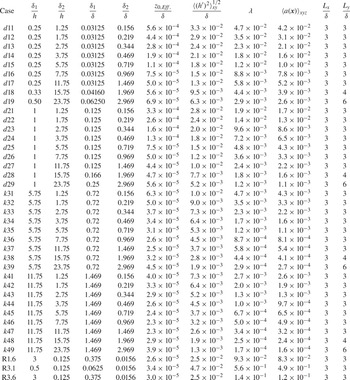
In order to address the role of canopy element distributions, we assembled the cases summarised in table 1. We systematically address the role of  $\delta _1$ and
 $\delta _2$ by fixing the former and varying the latter over targeted values known to encompass critical values of the parameter space. Figure 1 is a schematic of synthetic canopy arrangements, and provides graphical depiction of
 $\delta _1$ and
 $\delta _2$. We quantify flow response to spanwise heterogeneity (
 $\delta _2)$ for
 $k$- and
 $d$-type roughness (
 $\delta _1$). Given the large number of cases, we define table 1 case names via concatenation of three symbols:
 \begin{equation} \mathrm{Case} \equiv \underbrace{\left( \mathrm{Symbol}\ 1\right)}_{\substack{\mathrm{Roughness}\\k\ \mathrm{or}\ d-\mathrm{type}}} \quad \underbrace{\left( \mathrm{Symbol}\ 2\right)}_{\substack{\mathrm{Streamwise\ spacing}, \delta_1\\1\ \mathrm{to}\ 4}} \quad \underbrace{\left( \mathrm{Symbol}\ 3\right)}_{\substack{\mathrm{Spanwise\ spacing}, \delta_2\\1 \ \mathrm{to} \ 9}}. \end{equation}
The underbrace text summarises the parameter corresponding with each symbol. For these cases, we report  $\lambda$ and
 $\langle a ({\boldsymbol x}) \rangle _{xyz}$ in table 1. For all cases, the streamwise, spanwise and vertical extent of trees canopies is
 $h_1/\delta = 0.03125$,
 $h_2/\delta = 0.03125$ and
 $h_c/\delta = 0.075$, respectively, whereas the tree ‘trunks’ are squares with side length,
 $d_t/\delta = 0.0156$. For the cases considered, with
 $\delta /h = 8$, the large elements induce vortical motions that precludes assumption of outer-layer similarity (Townsend Reference Townsend1976). Turbulence statistics shown in the following section attenuate monotonically towards the domain centreline, indicating adequate resolution and no unphysical numerical effects associated with the prescribed boundary conditions. In table 1,
 $z_{0,{Eff.}}/\delta$ and
 ${\langle (h^\prime )^2 \rangle _{xy}^{1/2}}/{\delta }$ denote effective roughness length and root mean square (r.m.s.) of the height distribution, respectively, where
 $h^\prime = h - \langle h \rangle _{xy}$.


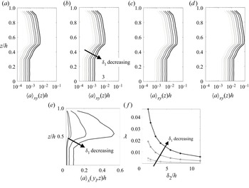
Figure 2 shows vertical profiles of canopy geometric attributes for all cases summarised in table 1 (with the exception of the comparison cases). Figure 2(a–d) shows vertical profiles of plane-averaged LAI,  $\langle \alpha ({\boldsymbol x}) \rangle _{xy}(z)$, for cases
 $k1i$ (a),
 $k2i$ (b),
 $d3i$ (c) and
 $d4i$ (d). In these panels, the direction of decreasing
 $\delta _1$ is shown, where it is apparent that leaf-area density monotonically increases as spanwise spacing declines. This is physically interpreted as relatively larger spatial volumes occupied by vegetation. In contrast, from panels (a) to (d)
 $\langle \alpha ({\boldsymbol x}) \rangle _{xy}(z)$ monotonically declines, owing to the relatively smaller spatial volumes occupied by vegetation. Figure 2(e) shows
 $\langle \alpha ({\boldsymbol x}) \rangle _{x}(y_l,z)$, where
 $y_l$ is coincident with the centre of a streamwise-aligned row of trees (given the sampling at
 $y_l$, panel (e) is insensitive to spanwise spacing and captures only variability in
 $\delta _1$). Finally, figure 2(f) shows the LAI,
 $\lambda$, for all cases in table 1 (with the exception of the comparison cases). Each datapoint on panel (f) corresponds with a case, and solid lines are used to ‘group’ cases with fixed
 $\delta _1$. These graphical illustrations of canopy geometric attributes are helpful in demonstrating consistent, monotonic trends with variation in
 $\delta _1$ and
 $\delta _2$ (see also figure 1 and (2.3) for canopy schematic and case code equation, respectively).
Vertical profiles of canopy geometric attributes for cases considered in this study. Panels (a–d) show vertical profiles of plane-averaged leaf-area density averaged for cases  $k1i$ (a),
 $k2i$ (b),
 $d3i$ (c) and
 $d4i$ (d), where index
 $i$ varies between 1 and 9 for variable
 $\delta _2$ (see also table 1 and (2.3)), and where an annotation for the direction of decreasing
 $\delta _1$ has been superimposed for perspective. Panel (e) shows streamwise-averaged leaf-area density at spanwise location,
 $y_l$, coincident with the centre of a row of trees, where an annotation for direction of
 $\delta _1$ is provided. Panel (f) shows the LAI,
 $\lambda$ (2.2), for all table 1 cases (with the exception of the comparison cases), with the direction of decreasing
 $\delta _1$ indicated.

In order to demonstrate efficacy of the present LES code, we have also modelled ASL flow over cases R1.6, R3.1 and R3.6, with attributes summarised in table 1. These cases are identical to those already considered by Bailey & Stoll (Reference Bailey and Stoll2013). Comparison of results from the present LES code against those reported previously by an independent group help to establish efficacy of the numerical approach; comparison results are shown in the Appendix. It is also noted that the LES code has now been in use for several decades and has been successfully used in a variety of research avenues.
For all cases, we used  $L_x/\delta = 3$ and
 $L_z/\delta = 1$, with
 $\delta /h = 8$;
 $L_y/\delta$ was varied to accommodate the canopy attributes, as recorded in table 1. This value of
 $\delta /h$ is sufficient to ensure that the flow is dominated by roughness sublayer dynamics, with no capacity for large-scale correlation in the outer layer (Raupach et al. Reference Raupach, Antonia and Rajagopalan1991, Reference Raupach, Finnigan and Brunet1996; Ghisalberti Reference Ghisalberti2009; Anderson, Li & Bou-Zeid Reference Anderson, Li and Bou-Zeid2015b). For this reason, the domain streamwise extent imposes no unphysical truncation of energy-containing large-scale motions, because roughness sublayer processes preclude emergence of outer-layer correlation (Hutchins & Marusic Reference Hutchins and Marusic2007). The computational domain is discretised with
 $\{N_x, N_y, N_z \} = \{192, 192, 160 \}$, which is consistent with Bailey & Stoll (Reference Bailey and Stoll2013).
3. Results
A series of results are presented to address the underlying question on secondary flow polarity in high-Reynolds-number channel flows over spanwise- and streamwise-heterogeneous canopies. As noted in § 1.1, this issue has been the topic of a sustained research effort regarding the polarity of roughness-driven secondary flows; that is, contrasting the results from Ganapathisubramani and coworkers (Vanderwel & Ganapathisubramani Reference Vanderwel and Ganapathisubramani2015; Medjnoun et al. Reference Medjnoun, Vanderwel and Ganapathisubramani2018, Reference Medjnoun, Vanderwel and Ganapathisubramani2020) against those from Anderson, Christensen, and others (Willingham et al. Reference Willingham, Anderson, Christensen and Barros2013; Barros & Christensen Reference Barros and Christensen2014; Anderson et al. Reference Anderson, Barros, Christensen and Awasthi2015a; Pathikonda & Christensen Reference Pathikonda and Christensen2017; Yang & Anderson Reference Yang and Anderson2017a; Awasthi & Anderson Reference Awasthi and Anderson2018; Zheng & Anderson Reference Zheng and Anderson2021). Results will demonstrate that, indeed,  $k$- or
 $d$-type roughness can regulate the polarity of roughness-driven secondary flows, where the former and latter induce upwelling and downwelling aloft streamwise-aligned roughness ‘rows’, respectively. This ability to regulate polarity is pronounced only in the transitional zone (based on
 $\delta _2$).
In order to efficiently present flow visualisations, we show instantaneous and Reynolds-averaged flow visualisations for cases spanning the transitional regime with respect to  $\delta _2$ and the
 $d$- and
 $k$-type regimes; indeed, the cases were designed a priori for precisely this reason. Results are shown in the spanwise–wall-normal plane, to illustrate large-scale flow response. Figures 3 and 4 show instantaneous and time-averaged results, respectively, for cases noted in the caption.
Contours of instantaneous streamwise velocity in the  $y$–
 $z$ plane at
 $x = L_x/2$, with isocontours of vertical velocity superimposed for values,
 $\tilde {w}({\boldsymbol x},t)/u_* = 1$ (red) and
 $-$1 (blue). Results are shown for table 1 cases with
 $\delta _2/\delta = 1.5$ and
 $\delta _1/h = 0.25$ (
 $d$17, panel a),
 $\delta _1/h = 5.75$ (
 $k$37, panel b) and
 $\delta _1/h$ = 11.75 (
 $k$47, panel c). Canopy elements are denoted with green silhouettes.

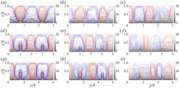
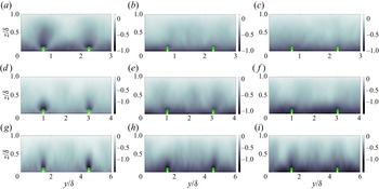
Contours of Reynolds-averaged streamwise velocity in the  $y$–
 $z$ plane at
 $x = L_x/2$, with isocontours of vertical velocity superimposed for values,
 $\langle \tilde {w} \rangle _t ({\boldsymbol x})/u_* = 1$ (red) and
 $-1$ (blue). Results are shown for table 1 cases with
 $\delta _2/\delta = 1.5$ (a–c show results for cases
 $d$17,
 $k$37 and
 $k$47), 2 (d–f show results for cases
 $d$18,
 $k$38 and
 $k$48) and 3 (g–i show results for cases
 $d$19,
 $k$39 and
 $k$49) and streamwise spacing
 $\delta _1/h = 0.25$ (a,d,g), 5.75 (b,e,h) and 11.75 (c,f,i). Canopy elements are denoted with green silhouettes.

For case  $d$17, with the lowest
 $\delta _1/h$, streamwise spacing between successive elements is
 $\delta _1/h = 0.25$, the flow is expected to ‘skim’ over successive elements in a manner that precludes intra-canopy flow reattachment (Macdonald et al. Reference Macdonald, Griffiths and Hall1998; Jimenez Reference Jimenez2004) (figure 3a). In contrast, the corresponding spanwise spacing,
 $\delta _2/\delta = 1.5$, is in the transitional regime (figure 1c and accompanying text). For case
 $d$17, figure 3(a) shows the large-scale fluctuation typical of instantaneous visualisation. Note, however, pronounced regions of relative streamwise momentum deficit and corresponding upwelling (red). This modality is also observed for case
 $k$37, which is in the
 $d$- to
 $k$-type transition region. The structure observed in figure 3(a,b), though based only on instantaneous visualisation, is consistent with results from Ganapathisubramani and coworkers (Vanderwel & Ganapathisubramani Reference Vanderwel and Ganapathisubramani2015; Medjnoun et al. Reference Medjnoun, Vanderwel and Ganapathisubramani2018, Reference Medjnoun, Vanderwel and Ganapathisubramani2020). However, for case
 $k$47 (figure 3c), for which
 $\delta _1/h = 11.75$ and the elements are thoroughly within the
 $k$-type regime, regions of aggregate momentum excess reside aloft the row of trees, a polarity reversal from the observations presented in figure 3(a,b).
Figure 4 provides further insight on secondary flow structure via Reynolds-averaged results. The top, middle and bottom row of panels corresponds with  $\delta _2/\delta = 1.5$, 2 and 3, respectively, whereas the left, middle and right column correspond with
 $\delta _1/h = 0.25$, 5.75 and 11.75, respectively. For the clear
 $d$-type cases (panels a,d,g), note that upwelling occurs only for
 $\delta _2/\delta = 1.5$ (panel a); for cases with relatively larger
 $\delta _2/\delta$, i.e. clearly within the topography regime, downwelling is observed above the panels, with upwelling concentrated only in the roughness sublayer region of the elements.
For cases with intermediate streamwise heterogeneity ( $k$37,
 $k$38 and
 $k$39, shown in figure 4b, e and h, respectively), upwelling is observed only for the case with the smallest spanwise heterogeneity (panel b). For cases with relatively larger spanwise heterogeneity, upwelling is concentrated within the roughness sublayer, but this is encompassed within a region of downwelling. Note also that for case
 $k$37, the domain-scale upwelling corresponds with a region of relative streamwise momentum deficit, whereas for cases
 $k$38 and
 $k$39, downwelling corresponds with a relative streamwise momentum excess. The latter modality represents a high-momentum pathway (HMP), as per Christensen and colleagues (Barros & Christensen Reference Barros and Christensen2014), whereas the former is consistent with findings from Ganapathisubramani and coworkers (Vanderwel & Ganapathisubramani Reference Vanderwel and Ganapathisubramani2015; Medjnoun et al. Reference Medjnoun, Vanderwel and Ganapathisubramani2018, Reference Medjnoun, Vanderwel and Ganapathisubramani2020). This result illustrates the significant extent to which both streamwise and spanwise heterogeneity regulate secondary flow modality.
For the very largest streamwise heterogeneity (figure 4c,f,i), downwelling occurs above the roughness elements for all cases: this can be appreciated by coincident downwelling and relative streamwise momentum excess. Based only upon figure 4, a relative demarcation in secondary flow modality could be envisioned between cases  $d$17 and
 $k$37 above and those below. As the results discussion advances, we show that both modalities are a manifestation of the same underlying flow physics: relative spatial imbalances of production and dissipation of turbulent kinetic energy,
 $tke({\boldsymbol x}) = (1/2)(\langle \tilde {\boldsymbol u}^\prime \rangle _t ({\boldsymbol x}) {\boldsymbol :} \langle \tilde {\boldsymbol u}^\prime \rangle _t ({\boldsymbol x}) + \mathrm {Tr}(\langle {\boldsymbol \tau } \rangle _t ({\boldsymbol x})))$, that necessitate Reynolds-averaged secondary cells, a mechanism first identified by Hinze (Reference Hinze1967). Under this framework, a relative space-local excess in
 $tke$ production necessitates entrainment of relatively low-
 $tke$ fluid. In the present context, the relative excesses occur above the streamwise-aligned rows. For brevity, and because
 $tke$ has been shown in complementary prior articles (Zheng & Anderson Reference Zheng and Anderson2021),
 $tke$ contours are not shown here. We have prepared targeted results of total streamwise–wall-normal turbulent stress, which is indicative of
 $tke$ in rough wall channel turbulence.
For the  $d$-type cases wherein the flow skims across the elements and the roughness sublayer depth is elevated, as per figure 4(a,b), the region of low-
 $tke$ fluid resides between the adjacent rows of trees, thereby requiring lateral entrainment. For reference, note that the roughness sublayer is defined here as the region over which element-driven upwelling occurs (Goldstein & Tuan Reference Goldstein and Tuan1998). For the
 $k$-type cases, in contrast, vortical mixing between successive streamwise-aligned trees and penetration of the canopy enables a relatively smaller roughness sublayer. As such, low-
 $tke$ fluid resides aloft, enabling downwelling (discussion to follow).
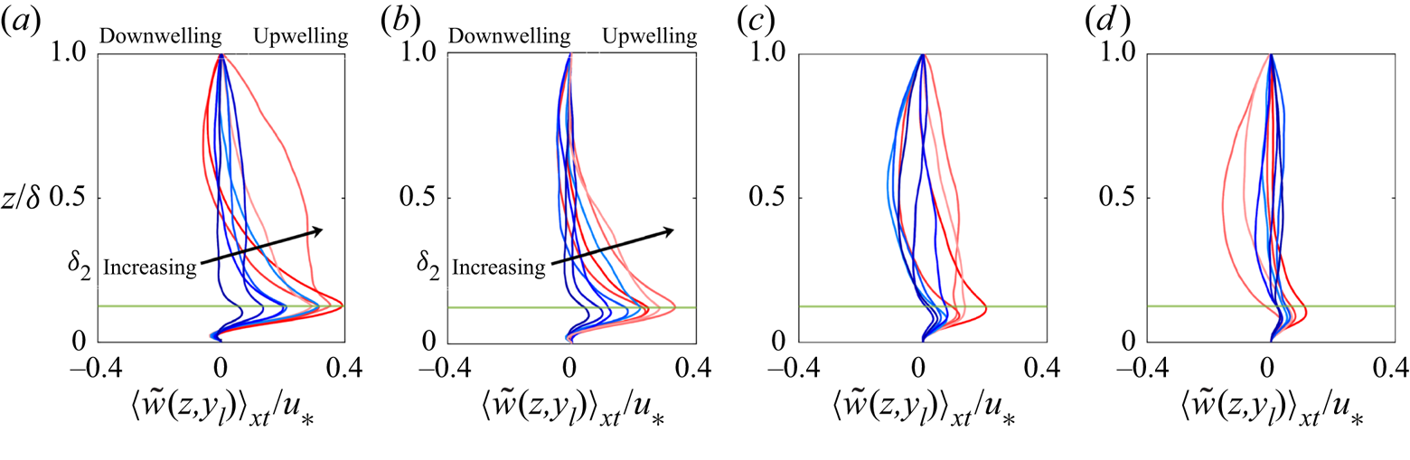
To further the discussion, figure 5 shows vertical profiles of vertical velocity for all table 1 cases, with the exception of the benchmark comparison cases, where panels (a–d) show profiles for cases  $d1i$,
 $d2i$,
 $k3i$ and
 $k4i$, respectively. The profiles are recovered from a spanwise location coincident with the centre of a row of elements, and downwelling and upwelling annotations are provided for perspective.
Vertical profiles of  $x$- and Reynolds-averaged vertical velocity at spanwise location,
 $y_l$, coincident with the centre of a row of trees. Panels (a–d) show results for cases
 $d1i$,
 $d2i$,
 $k3i$ and
 $k4i$, respectively, where
 $i = 1$–9 corresponds with a colour transition from red to blue. Annotations superimposed for downwelling and upwelling. The canopy elevation,
 $h/\delta$, is denoted by horizontal green lines, and the direction of increasing
 $\delta _2$ is shown for perspective.

For the  $d$-type cases (figure 5a,b), the magnitude of the vertical gradient of vertical velocity increases monotonically with increasing
 $\delta _2$; in addition, apparent depth of the roughness sublayer thickens with increasing
 $\delta _2$, which is consistent with growth of the roughness sublayer vortices with growing
 $\delta _2$ (Yang & Anderson Reference Yang and Anderson2017b; Anderson et al. Reference Anderson, Yang, Shrestha and Awasthi2018). This pattern of upwelling aloft the elements occurs for both
 $d$-type cases; for the
 $k$-type cases: the vertical gradients of vertical velocity are significantly smaller by virtue of the larger streamwise distances between successive elements. This is evidence of the aforementioned ‘lowering’ of the roughness sublayer to occupy the canopy: the intensity of canopy-driven mixing and associated upwelling from canopy elements declines monotonically from the
 $d$- to
 $k$-type cases. Note also that for the
 $k$-type cases the regions of downwelling emerge for cases with larger spanwise heterogeneity (darker profiles). This is consistent with aforementioned secondary flow polarity reversal as topographic attributes vary.
In seminal work, Reynolds-averaged secondary flows due to spatial heterogeneity of turbulent stresses, so-called Prandtl's secondary flow of the second kind, were first interpreted via the balance of  $tke$ (Hinze Reference Hinze1967) (for a review, see Bradshaw Reference Bradshaw1987 and references therein). In the context of hydraulic flows over beds with spanwise-variable hydrodynamic roughness, Vermaas et al. (Reference Vermaas, Uijttewaal and Hoitink2011) adopted the arguments of Hinze (Reference Hinze1967) to interpret secondary flow polarity (Wang & Cheng Reference Wang and Cheng2005). More recently, Anderson et al. (Reference Anderson, Barros, Christensen and Awasthi2015a) adopted the framework set forth by Hinze (Reference Hinze1967) to explain secondary flow attributes in high-Reynolds-number rough-wall boundary layers and channels. Prandtl's secondary flow of the second kind can be readily understood via the Reynolds-averaged
 $tke$ balance:
 \begin{equation} \langle \tilde{v} \rangle_{1t} \partial_y tke + \langle \tilde{w} \rangle_{1t} \partial_z tke = \mathcal{P} - \epsilon, \end{equation}
where the first and second terms on the right-hand side are production and dissipation, respectively. Application of (3.1) over a vertical profile at a spanwise transect coincident with a row of trees, the first left-hand side term vanishes. Recall that  $\mathcal {P} = \langle {\boldsymbol u}^\prime \otimes {\boldsymbol u}^\prime \rangle _{xt} {\boldsymbol :} \boldsymbol {\nabla } \langle {\boldsymbol u} \rangle _{xt}$, where
 ${\boldsymbol u}^\prime = {\boldsymbol u} - \langle {\boldsymbol u} \rangle _{xt}$ and where
 ${\boldsymbol{\mathsf{T}}} = {\boldsymbol u}^\prime \otimes {\boldsymbol u}^\prime$ is the Reynolds (total) stress tensor (in the LES context, recovered via addition of the resolved and subgrid-scale stresses). It is self-evident that for the present channel flows,
 ${\boldsymbol u}^\prime \otimes {\boldsymbol u}^\prime$ is dominated by the streamwise–wall-normal component whereas
 $\boldsymbol {\nabla } \langle {\boldsymbol u} \rangle _{xt}$ is dominated by the wall-normal gradient of streamwise velocity, i.e.
 $\mathcal {P} \approx \langle {\mathsf {T}}_{xz} \rangle _{xt} \partial _z \langle u \rangle _{xt}$. Above the elements, intense shear leads production of
 $tke$ to exceed dissipation, automatically imposing
 $\mathcal {P} - \epsilon > 0$. Irrespective of the magnitude of
 $tke$ above the elements, the vertical gradient of
 $tke$ must be negative, subsequently necessitating downwelling in order to match the polarity of the left- and right-hand side. It is emphasised that this framework has been used rigorously in prior, complementary studies (Wang & Cheng Reference Wang and Cheng2005; Vermaas et al. Reference Vermaas, Uijttewaal and Hoitink2011; Anderson et al. Reference Anderson, Barros, Christensen and Awasthi2015a; Salesky, Calaf & Anderson Reference Salesky, Calaf and Anderson2022). For this reason, we have not repeated the exercise here, and rather have used qualitative attributes of the
 $tke$ balance to establish context for the observations. Note also that other researchers have considered how imbalances in production and dissipation aloft flows over horizontally homogeneous canopies affect the hierarchy of dynamically active scales present and associated normalising length scales (Pan & Chamecki Reference Pan and Chamecki2016; Ghannam et al. Reference Ghannam, Katul, Bou-Zeid, Gerken and Chamecki2018).
Figure 6 shows contours of total streamwise–wall-normal stresses,  $\langle {\mathsf {T}}_{xz} \rangle _{xt}/u_*^2$, for the same cases highlighted in figure 4, where
 $\delta _1$ and
 $\delta _2$ increases in the left-to-right and top-to-bottom directions, respectively; recall that
 $u_{*}^2 = \max \langle | \tilde {u}^\prime \tilde {w}^\prime | \rangle _t ({\boldsymbol x}) + \max \langle | \tau _{xz} | \rangle _t ({\boldsymbol x})$ (Bailey & Stoll Reference Bailey and Stoll2013). Note that for the figure 4 cases that exhibited upwelling,
 $d$-type cases with smallest
 $\delta _2$, we see corresponding
 $\delta$-scale plumes of elevated
 ${\mathsf {T}}_{xz}$ throughout the domain (figure 6a,b). In contrast, for cases with established downwelling aloft the elements, the plume of elevated
 ${\mathsf {T}}_{xz}$ resides within the canopy. When viewed through the framework established by Hinze (Reference Hinze1967), the
 $d$-type modality (figures 6a,b) can be understood as inducing a region of elevated
 $\mathcal {P}$ that is so large that entrainment from aloft is not possible; instead,
 $tke$ can be optimally balanced via lateral entrainment. In contrast, when the roughness sublayer occupies the canopy, as it does for the
 $k$-type response, the region of elevated
 ${\mathsf {T}}_{xz}$ is relatively smaller. With this, regions of elevated
 $\mathcal {P}$ are confined to the canopy, providing greater spatial extent for entrainment of low-
 $tke$ fluid from aloft (discussion to follow).
Contours of  $x$- and Reynolds-averaged streamwise–wall-normal Reynolds (turbulent) stresses,
 $\langle {\mathsf {T}}_{xz} \rangle _{xt}/u_*^2 = (\langle \tilde {u}^\prime \tilde {w}^\prime \rangle _{xt} + \langle \tau _{xz} \rangle _{xt})/u_*^2$, in the
 $y$–
 $z$ plane. Results are shown for table 1 cases with
 $\delta _2/\delta = 1.5$ (a–c shows results for cases
 $d$17,
 $k$37 and
 $k$47), 2 (d–f shows results for cases
 $d$18,
 $k$38 and
 $k$48) and 3 (g–i shows results for cases
 $d$19,
 $k$39 and
 $k$49) and streamwise spacing
 $\delta _1/h = 0.25$ (a,d,g), 5.75 (b,e,hs) and 11.75 (c,f,i). Canopy elements are denoted with green silhouettes.

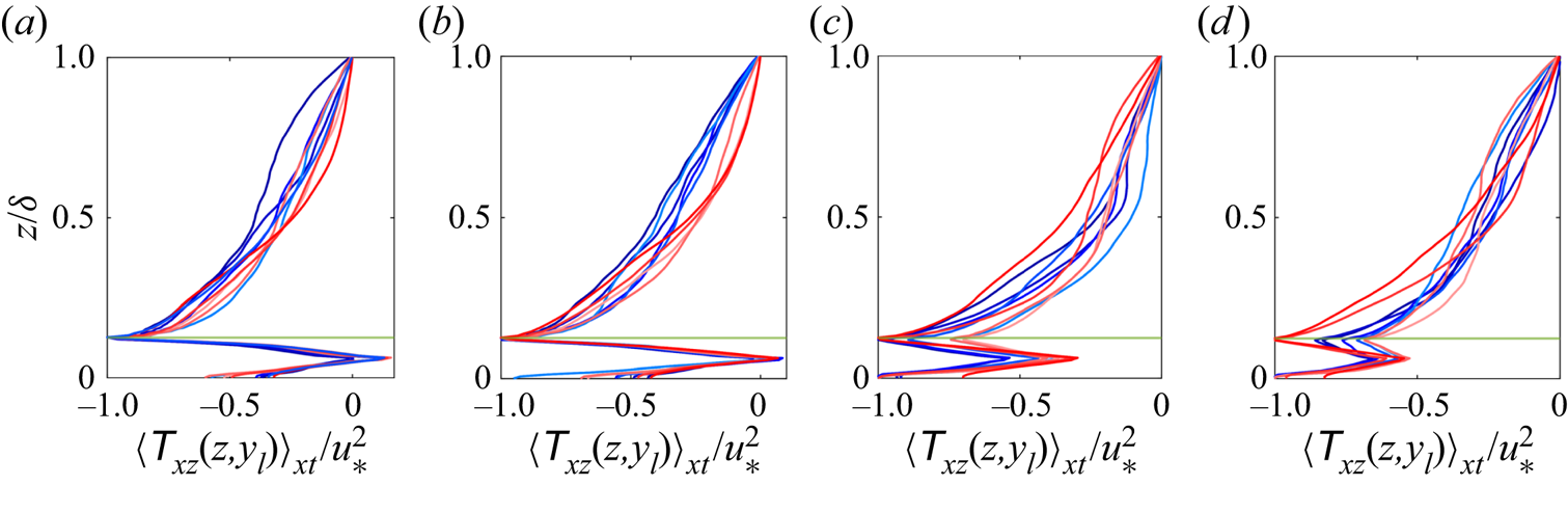
To provide more clarity on figure 6 and accompanying discussion, in figure 7 we show vertical profiles of  $\langle {\mathsf {T}}_{xz} \rangle _{xt} (y_l, z)$, where
 $y_l$ is a spanwise location coincident with the centreline of a row of trees. As per figure 5, a horizontal green profile has been superimposed to denote the elevation of the canopy. For the
 $d$-type cases, as might be expected, the shear layer is most intense at
 $h/\delta$ (figure 7a,b); in contrast, for the
 $k$-type cases, elevated shear occurs throughout the canopy, and generally attains its maximum value at the wall, indicative of declining fluxes of momentum to the canopy with increasing
 $\delta _1$.
Vertical profiles of  $x$- and Reynolds-averaged streamwise–wall-normal Reynolds (turbulent) stresses,
 $\langle {\mathsf {T}}_{xz} \rangle _{xt} = \langle \tilde {u}^\prime \tilde {w}^\prime \rangle _{xt} + \langle \tau _{xz} \rangle _{xt}$, at spanwise location,
 $y_l$, coincident with the centre of a row of trees. Panels (a–d) show results for cases
 $d1i$,
 $d2i$,
 $k3i$ and
 $k4i$, respectively, where
 $i = 1$ to 9 corresponds with a colour transition from blue to red. The canopy elevation,
 $h/\delta$, is denoted by horizontal green lines.

Note that because the profiles are shown at a discrete spanwise location, there is no means to incorporate the dispersive stress component, that is, stresses due to spatial heterogeneity of the mean flow, as per Calaf, Meneveau & Meyers (Reference Calaf, Meneveau and Meyers2010) or Bailey & Stoll (Reference Bailey and Stoll2013). In separate work, we have computed vertical profiles of the plane-averaged stresses, which recovered the expected linearly decreasing profile. The profiles observed in figure 7 are a consequence of flow response to the canopy attributes.
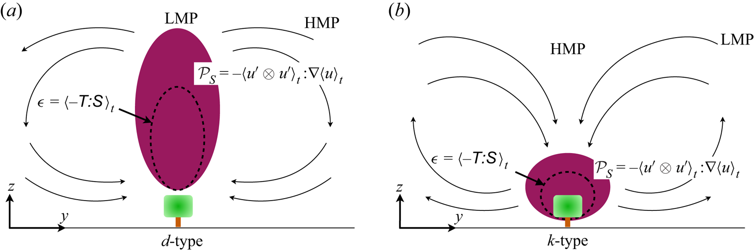
Figure 8 is an illustrative depiction of the aforementioned  $tke$ balance mechanisms responsible for the observed secondary flow polarity reported in figures 3 and 4. For the
 $d$-type cases, the relatively small values of
 $\delta _1$ prevent the canopy-driven shear layer from occupying the canopy, and instead production of turbulence occurs over the depth of the flow (figure 8a). This precludes entrainment of low-
 $tke$ fluid from aloft, thereby necessitating lateral entrainment. This explains the observed low-momentum pathway above the elements for
 $d$-type cases (Barros & Christensen Reference Barros and Christensen2014). For the
 $k$-type cases, regions of elevated
 $tke$ production occupies the canopy (figure 8b), which enables lateral entrainment from aloft and formation of HMPs above the elements.
Idealised depiction of  $tke$ production and dissipation dynamics for the
 $d$- (a) and
 $k$-type cases (b), respectively. Red regions denote locations of elevated production, dashed grey denotes regions of elevated dissipation.

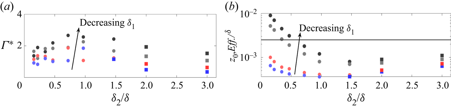
To conclude the present discussion, figure 9(a) presents datapoints for compensated circulation:
 \begin{equation} \varGamma^* = \dfrac{\varGamma}{u_* \delta} = \displaystyle\int_{{d}^2 {\boldsymbol x}} | \langle \tilde{\omega}_x \rangle_{xt} (y,z) | \,\mathrm{d} {y} \,\mathrm{d} {z}, \end{equation}
as per Yang & Anderson (Reference Yang and Anderson2017b), and figure 9(b) presents datapoints for a posteriori-recovered effective roughness length,  $z_{0,{Eff.}}/\delta$. Each datapoint corresponds with a table 1 simulation, as per the caption, with the notable exception of the benchmark comparison cases, which are utilised in the Appendix.
Bulk flow attributes for table 1 simulations. Panels (a,b) show compensated circulation,  $\varGamma ^*$ (3.2) and effective roughness length,
 $z_{0,{Eff.}}/\delta$, respectively, shown against spanwise heterogeneity,
 $\delta _2/\delta$. Symbols correspond with
 $\delta _1/h$ =
 $0.25$ (black symbols),
 $1$ (grey symbols),
 $5.75$ (red symbols) and
 $11.75$ (blue symbols); direction of decreasing
 $\delta _1$ superimposed for perspective. Cases with upwelling and downwelling above a row of elements are denoted with filled circles and filled squares, respectively. In panel (b), the horizontal solid line shows base roughness length,
 $\hat {z}_0/\delta$.

Compensated circulation is a helpful bulk metric for quantifying intensity of roughness-driven secondary flows; in the absence of spanwise heterogeneity, or for infinite spanwise heterogeneity,  $\varGamma ^* = 0$. Between these limiting values of
 $\delta _2$,
 $\varGamma ^*$ varies, where interested readers may consult Yang & Anderson (Reference Yang and Anderson2017b) or Anderson et al. (Reference Anderson, Yang, Shrestha and Awasthi2018) for further discussion.
In figure 9(a), the datapoints exhibit non-monotonic dependence on  $\delta _2$, which has been reported in numerous preceding articles (Yang & Anderson Reference Yang and Anderson2017b; Anderson et al. Reference Anderson, Yang, Shrestha and Awasthi2018); it is noted that Medjnoun et al. (Reference Medjnoun, Vanderwel and Ganapathisubramani2018) have also qualitatively defined this with their ‘significance’ parameter. These trends can be interpreted as growing secondary flow intensity in the roughness regime (recall figure 1c), as the element-driven secondary flows in the
 $d$-type regime grow in spatial extent with increasing
 $\delta _2$. This trend asymptotes in the transitional regime, before reversing trend. This is a consequence of the secondary cells occupying a relatively lesser spatial extent, and with the emergence of HMPs and their relatively lower streamwise vorticity (figure 8 and accompanying text). The symbol colour codes denote the respective values of
 $\delta _1$, and the direction of decreasing
 $\delta _1$ is superimposed, for perspective.
As might be anticipated, as  $\delta _1$ decreases, the topography becomes relatively ‘more rough’ and the element-driven secondary cells exhibit more intense compensated circulation. This trend, and the asymptotic turning point for
 $\delta _2/\delta \approx 1$, is invariant to
 $d$- or
 $k$-type values. Note that on figure 9(a), filled circles and filled squares correspond with cases that exhibit Reynolds-averaged upwelling or downwelling, respectively. Recall that the latter, downwelling aloft the elements, corresponds with antecedent observations of HMPs reported by Christensen, Anderson, and others (i.e. Willingham et al. Reference Willingham, Anderson, Christensen and Barros2013; Barros & Christensen Reference Barros and Christensen2014; Anderson et al. Reference Anderson, Barros, Christensen and Awasthi2015a). Detailed inspection of figure 9(a) reveals that secondary flow polarity reverses for the
 $k$-type cases first (blue square at
 $\delta _2/\delta \approx 1.5$), whereas all cases reverse for larger
 $\delta _2/\delta$. This is evidence of the aforementioned polarity reversal for larger
 $\delta _1$, as the production–dissipation imbalance occupies the canopy.
Figure 9(b) shows effective roughness length normalised by flow depth,  $z_{0,{Eff.}}/\delta$, which is recovered a posteriori via least-squares fit of a logarithmic (equilibrium) profile to vertical profiles of plane- and time-averaged streamwise velocity,
 $\langle \tilde {u} \rangle _{xyt}/u_*$. The least-squares fit is based on data over the range,
 $0.4 \leq z/\delta \leq 0.8$. Given that the effective roughness lengths are based on a rigorous least-squares fit, and the strong trends observed on the panels, the reported values of
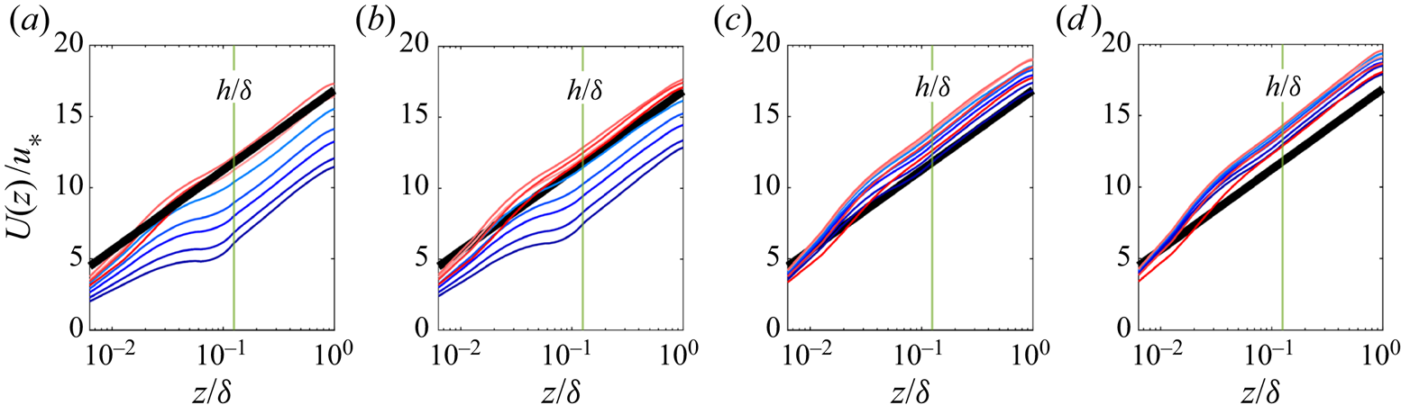
 $z_{0,{Eff.}}$ may be regarded as robust and accurate. To provide support for these results, please note that figure 10 shows vertical profiles for plane- and time-averaged streamwise velocity. For all cases, it is clear that a well-established logarithmic region is present, evidenced by comparison against the superimposed idealised profile. For perspective, the elevation of the canopy elements is superimposed; an idealised logarithmic profile (thick black) is superimposed, which illustrates that the aforementioned protocol for recovery of
 $z_{0,{Eff.}}$ is efficacious.
Vertical profiles of plane- and Reynolds-averaged streamwise velocity,  $U(z) = \langle \tilde {u} \rangle _{xyt} (z)$. Panels (a–d) show results for cases
 $d1i$,
 $d2i$,
 $k3i$ and
 $k4i$, respectively, where
 $i = 1$–9 corresponds with a colour transition from red to blue. The canopy elevation,
 $h/\delta$, is denoted by vertical green line and annotation. An idealised logarithmic profile based on roughness length,
 $z_0/\delta = 10^{-3}$, is superimposed for perspective.

On figure 9(b), the direction of decreasing  $\delta _1$ is superimposed, for context, and as expected the roughness length increases monotonically with decreasing
 $\delta _1$. This can be understood as a direct consequence of additional drag associated with larger leaf area index (recall also figure 2). Similarly, for the roughness-regime cases (
 $d$- and
 $k$-type), effective roughness decreases monotonically as spanwise spacing increases and leaf area index declines. This trend reverses for transitional cases and tends toward increasing roughness for yet-larger
 $\delta _2$. Recall, however, that it is these cases for which the distinct HMPs emerge and persistent downwelling occurs above the elements due to the production–dissipation imbalance and entrainment of low-
 $tke$ fluid. Thus, the entrainment of relatively high-momentum fluid from aloft manifests as an added drag. It is noted, also, that the onset of this is reported for the largest
 $\delta _1$ case, when the associated roughness sublayer occupies the greatest spatial extent of the canopy. On figure 9(b), the base roughness,
 $\hat {z}_0/\delta$, prescribed in the LES (alongside the bluff canopy elements; § 2.1) is shown via horizontal black line. As expected, as
 $\delta _2$ increases, noting that the limit,
 $\delta _2 = \infty$, corresponds with a homogeneous roughness length,
 $\hat {z}_0$, we see tendency towards
 $\hat {z}_0$.
3.1. $k$- and $d$-type roughness, flow response


The results in figure 9(b) can be interpreted somewhat differently by quantifying the correlation between effective roughness length and corresponding canopy attributes. One such correlation, which has received widespread use over many years (Garratt Reference Garratt1994; Zagarola & Smits Reference Zagarola and Smits1998) is:
 \begin{equation} z_{0,{Eff.}} (h, \delta_1, \delta_2) \sim \sigma_h = \alpha (\delta_1, \delta_2) \sigma_h + \hat{z}_{0}, \end{equation}
where  $\alpha$ is a proportionality constant relating height r.m.s.,
 $\sigma _h = (\langle h^2 \rangle _{xy} - \langle h \rangle _{xy}^2)^{1/2}$, and roughness length, and
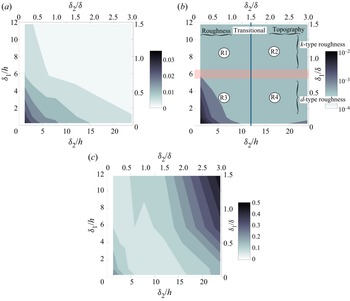
 $\hat {z}_{0}$ is the aforementioned ‘baseline’ roughness length (Anderson & Meneveau Reference Anderson and Meneveau2010b). Figure 11(a) shows a contour flood of
 $\sigma _h$ for the table 1 cases, with the exception of the benchmark comparison cases. As might be expected, the largest values occur for the smallest
 $\delta _1$ and
 $\delta _2$, and
 $\sigma _h$ decreases monotonically with increases in both.
Large-scale aerodynamic response to variable canopy attributes. Panels (a–c) show height r.m.s.,  $\sigma _h = ( \langle h^2 \rangle _{xy} - \langle h \rangle _{xy}^2 )^{1/2}$, a posteriori-recovered effective roughness length,
 $z_{0,{Eff.}}$, and (3.3) proportionality constant,
 $\alpha$, respectively (note that individual values for
 $\sigma _h$,
 $z_{0,{Eff.}}$ and
 $\alpha$ are recorded in table 1). Panel (b) illustrates how the confluence of variable
 $\delta _1$ and
 $\delta _2$ preclude automatic surface regime description. Nominal regions where
 $\delta _2$ renders the surface a ‘roughness’ or ‘topography’ are shown (top and bottom abscissa) against regions where
 $\delta _1$ renders the surface
 $k$- or
 $d$-type (left and right ordinate), where
 $\delta _1$ and
 $\delta _2$ are defined with respect to flow depth and canopy height, for perspective. This confluence yields quadrant regions R1, R2, R3 and R4, which are graphically illustrated in figure 1(c).

Figure 11(b) shows the corresponding contour flood of  $z_0/\delta$ for the table 1 cases, where the idealised regimes depicted on figure 1(a) are superimposed for context. The elevated roughness contours for small
 $\delta _1$ and
 $\delta _2$ were already presented and discuss in figure 9(b), likewise the trend reversal and elevated values for small large
 $\delta _2$ and small
 $\delta _1$, as the secondary cells reverse and high momentum fluid is entrained toward the roughness elements. However, the contour of
 $\alpha (\delta _1, \delta _2)$ (figure 11c) provides detailed illustration of the roughness length and height r.m.s. correlate. Note that the minimal value required to correlate
 $z_0$ and
 $\sigma _h$ a priori manifests as a channel spanning cases with the smallest
 $\delta _2$ and largest
 $\delta _1$ to cases with the smallest
 $\delta _1$ and transitional
 $\delta _2$. The proportionality constant,
 $\alpha (\delta _1, \delta _2)$, was recovered via rearrangement of (3.3).
Cases with small  $\delta _2$ and large
 $\delta _1$ correspond with
 $k$-type arrangements, with spanwise spacing
 $k$-type cases, with spanwise spacing sufficiently small that vigorous mixing occurs within the canopy and the elements absorb the greatest fraction of the momentum flux; for smaller
 $\delta _1$, mixing within the canopy is attenuated and the relative efficiency of the correlation declines. As
 $\delta _2$ increases, thereby providing greater spatial extent within the canopy, and as
 $\delta _1$ decreases, element-driven mixing occupies the spatial ‘gaps’ between the streamwise-aligned row of elements. It is only for this relatively narrow range of the
 $\delta _1$–
 $\delta _2$ parameter space that vigorous mixing within the canopy corresponds with the smallest values of
 $\alpha$, and values of
 $\alpha$ closest to prior studies (Zagarola & Smits Reference Zagarola and Smits1998; Anderson & Meneveau Reference Anderson and Meneveau2011).
4. Conclusion
LES has been used to perform an assessment of turbulent channel flow response to rough canopies composed of virtual trees. The arrangements are carefully assembled to isolate flow response with variable streamwise and spanwise spacing, the former affecting  $d$- or
 $k$-type response, the latter affecting roughness, transition or topography response; no prior article has simultaneously addressed the role of both parameters. Consistent with prior articles, we find that for
 $\delta _2/\delta \lesssim 1$ (in the roughness regime), upwelling is persistent above the elements irrespective of the presence of a
 $d$- or
 $k$-type arrangement. However, in the transitional regime,
 $\delta _1$ regulates the onset of secondary flow polarity reversal and the emergence of established HMPs. For the asymptotic inertial conditions addressed herein, roughness element attributes are not expected to significantly alter the results, although subsequent work may well be needed to resolve this issue.
Funding
This work was supported by the National Science Foundation (grant no. AGS-1839929). Computational resources were provided by the Texas Advanced Computer Center at the University of Texas.
Declaration of interests
The authors report no conflict of interest.
Appendix. Comparison against benchmark datasets
In order to demonstrate efficacy of the LES code used for this article, we repeated the simulations first carried out by Bailey & Stoll (Reference Bailey and Stoll2013). Attributes for these cases are summarised in table 1 (R1.6, R3.1 and R3.6). For brevity, we show only targeted results here, which are shown in figure 12, where panel (a) shows vertical profiles of plane-averaged LAI, whereas panels (b,c) show plane- and time-averaged streamwise velocity and streamwise–wall-normal turbulent stresses. Figure 12(a) indicates that the cases have been correctly replicated; panels (b,c) illustrate agreement with the prior dataset, at least to the second order. These results provide support for results and accompanying scientific deductions presented throughout the main text.
Canopy attributes and resultant Reynolds-averaged flow statistics for cases R1.6, R3.1 and R3.6 (salient case details summarised in table 1; cases adopted from Bailey & Stoll Reference Bailey and Stoll2013). Panel (a) shows vertical profiles of leaf-area density; panels (b,c) show vertical profiles of plane- and time-averaged streamwise velocity and streamwise–wall-normal turbulent stresses, respectively. Solid lines show results from LES, whereas symbols show datapoints recovered from Bailey & Stoll (Reference Bailey and Stoll2013), where light grey, grey and black lines/symbols correspond with cases R3.1, R3.6 and R1.6, respectively.