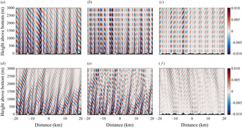
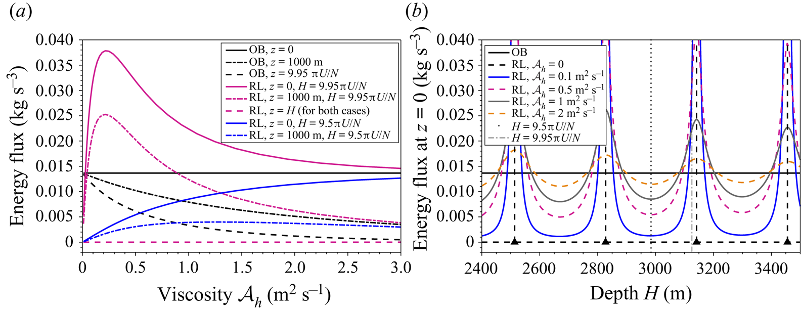
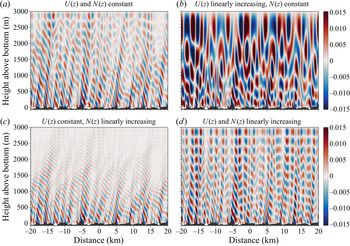
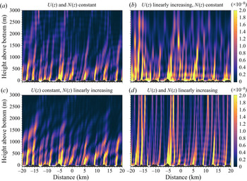
1. Introduction
Oceanic lee waves are quasi-steady internal gravity waves generated by the interaction of geostrophic flows with submarine topography. They are present throughout the world's oceans, accounting for an estimated 0.2–0.75 TW of conversion from the geostrophic flow (Nikurashin & Ferrari Reference Nikurashin and Ferrari2011; Scott et al. Reference Scott, Goff, Naveira Garabato and Nurser2011; Wright et al. Reference Wright, Scott, Ailliot and Furnival2014). Approximately half of this generation takes place in the Southern Ocean (SO) (Nikurashin & Ferrari Reference Nikurashin and Ferrari2011), where lee waves have been shown to be an important sink of energy and momentum from the energetic mesoscale eddies of the Antarctic Circumpolar Current (ACC) due to the rough topography and high bottom velocities in the region (Nikurashin & Ferrari Reference Nikurashin and Ferrari2010a; Nikurashin, Vallis & Adcroft Reference Nikurashin, Vallis and Adcroft2012; Naveira Garabato et al. Reference Naveira Garabato, Nurser, Scott and Goff2013; Yang et al. Reference Yang, Nikurashin, Hogg and Sloyan2018).
Lee waves play an important role not only in the momentum budget of the mean flow through lee wave drag, but also in the buoyancy and tracer budgets through diapycnal mixing. Enhanced levels of turbulence above topography associated with lee waves and other topographic interaction processes are an important source of diapycnal mixing in the deep ocean, contributing to the closure of the meridional overturning circulation (MacKinnon et al. Reference MacKinnon2017; Cessi Reference Cessi2019). The SO upwelling of tracers such as  $\mathrm {CO}_2$ and nutrients for primary production are also sensitive to mixing in the ocean, with important consequences for air–sea fluxes and ultimately climate (Talley et al. Reference Talley2016).
Lee wave horizontal length scales are typically of order 500 m–10 km in the ocean, a range that is unresolved in global climate models, so the mixing and drag effects of lee waves both need to be parametrised. The generation of lee waves is usually understood using linear theory, whereby the lee wave perturbations are assumed to have a much smaller amplitude than the mean flow itself (Bell Reference Bell1975). An important parameter determining the linearity of lee waves generated at topography of characteristic height  $h$ in uniform background stratification
 $N$ and flow speed
 $U$ is the lee wave Froude number
 $Fr_L = Nh/U$ (Mayer & Fringer Reference Mayer and Fringer2017). Lee waves can propagate vertically when their horizontal wavenumber
 $k$ (set by topography) is such that
 $|\,f| < |Uk| < |N|$, where
 $f$ is the Coriolis parameter. Under the assumption
 $|\,f| \ll |Uk| \ll |N|$,
 $Fr_L$ is proportional to the ratio of the topographic height
 $h$ to the lee wave vertical wavelength, or equivalently the ratio of the perturbation horizontal velocity to the background velocity, thus the linear approximation is formally valid for
 $Fr_L \ll 1$. Energy flux calculated using the linear approximation has been shown to agree with two-dimensional (2-D) nonlinear simulations for
 $Fr_L \lesssim {O}(1)$ (Nikurashin et al. Reference Nikurashin, Ferrari, Grisouard and Polzin2014).
For 2-D topography and flow conditions such that  $Fr_L$ is greater than some critical Froude number
 $Fr_L^{{crit}} \sim {O}(1)$, topographic blocking occurs since the flow lacks the kinetic energy to raise itself over a bump of height greater than
 $\sim U/N$ (Smith Reference Smith1989). Thus, the effective height of topography
 $h^{{eff}}$ is always reduced such that the waves are generated with
 $Fr_L^{{eff}} = Nh^{{eff}}/U \lesssim Fr_L^{{crit}}$ (Winters & Armi Reference Winters and Armi2012). When the topography is three-dimensional, splitting may also occur as the flow goes around rather than over a bump, and the effective height is lower still. Nikurashin et al. (Reference Nikurashin, Ferrari, Grisouard and Polzin2014) found that for multichromatic topography with
 $h$ defined as the r.m.s. (root mean square) topographic height,
 $Fr_L^{{crit}} \simeq 0.7$ for 2-D topography, and
 $Fr_L^{{crit}} \simeq 0.4$ for 3-D topography. Thus, with modifications for finite amplitude and 3-D effects, the linear theory can be used with some success even when the r.m.s. topographic height violates the linear approximation. Several estimates of energy conversion from the geostrophic flow to lee waves have been found using estimated topographic spectra, bottom velocities and stratification globally (Bell Reference Bell1975; Nikurashin & Ferrari Reference Nikurashin and Ferrari2011; Scott et al. Reference Scott, Goff, Naveira Garabato and Nurser2011; Wright et al. Reference Wright, Scott, Ailliot and Furnival2014). Problems remain with this approach, such as the proper representation of blocking in the topographic spectrum, and the neglect of the influence of flow due to large-scale topography on the radiating lee waves, which can significantly impact the dissipation above topography (Klymak Reference Klymak2018).
Although the generation of lee waves is well understood in a linear sense, the ultimate fate of lee wave energy as a fundamentally nonlinear and dissipative process is poorly constrained. After generation, lee waves radiate vertically and downstream away from topography. A vertical structure function exponentially decreasing with height above bottom was proposed by St. Laurent, Simmons & Jayne (Reference St. Laurent, Simmons and Jayne2002) for parametrisation of the dissipation rate due to the breaking of internal tides, and this has been implemented in lee wave parametrisations with decay scales between  $300$ and 1000 m (Nikurashin & Ferrari Reference Nikurashin and Ferrari2013; Melet et al. Reference Melet, Hallberg, Legg and Nikurashin2014). Both of these studies found that water mass transformation was sensitive to the decay scale used, thus accurate parametrisation of the vertical structure of mixing and dissipation is necessary for correctly predicting the ocean state in global climate models.
Lee waves also play an important role in causing drag on the flow, especially in the ACC (Naveira Garabato et al. Reference Naveira Garabato, Nurser, Scott and Goff2013; Yang et al. Reference Yang, Nikurashin, Hogg and Sloyan2018). When flow impinges on topography, the pressure differences across the topographic features cause drag, known as form drag. If there is topographic blocking, or the conditions for radiation of lee waves are not met, this drag will force the flow local to the topography. However, if lee waves are generated and propagate upwards this drag is distributed across the water column as a wave drag, locally forcing the flow where the waves break. Thus, the vertical distribution of the decelerating force on the mean flow due to lee wave breaking must also be parametrised. In the linear theory, the energy flux at topography is equal to the product of the total lee wave drag and the bottom background velocity, but the vertical distributions of the forcing on the flow and the energy loss need not be the same.
Possible sinks for lee wave energy include breaking due to vertical shear from inertial oscillations generated by parametric instability (Nikurashin & Ferrari Reference Nikurashin and Ferrari2010b), dissipation at critical levels (Booker & Bretherton Reference Booker and Bretherton1967), breaking due to convective instability on generation (Peltier & Clark Reference Peltier and Clark1979) and re-absorption of lee wave energy in a vertically sheared flow that decreases away from the topography (Kunze & Lien Reference Kunze and Lien2019). Nikurashin & Ferrari (Reference Nikurashin and Ferrari2010a) performed idealised simulations representative of lee wave generation and dissipation in the SO, finding that 50 % of lee wave energy dissipated in the bottom 1 km of the ocean for  $Fr_L \geq 0.5$ compared with 10 % for
 $Fr_L = 0.2$. A more realistic simulation capturing the characteristic stratification, wind forcing and topography of the SO (Nikurashin et al. Reference Nikurashin, Vallis and Adcroft2012) found that 80 % of the wind power input into geostrophic eddies was converted to smaller scales by topography, of which just 20 % radiated into the interior ocean, with most dissipated in the bottom 100 m. However, this and other wave resolving models may use artificially high diffusivity and viscosity, preventing lee waves from radiating in a physical way (Shakespeare & Hogg Reference Shakespeare and Hogg2017).
The linear theory of Bell (Reference Bell1975) uses a freely radiating upper boundary condition (hereafter referred to as ‘unbounded’ theory), and can only be applied for uniform stratification and velocity, or by using the Wentzel–Kramers–Brillouin (WKB) approximation in some cases (Gill Reference Gill1982; de Marez, Lahaye & Gula Reference de Marez, Lahaye and Gula2020). This has led most idealised oceanic lee wave studies to assume the same and treat lee waves as a process confined to the deep ocean where stratification and velocity are assumed to be approximately constant with height. The assumption in most such studies (with some exceptions, e.g. Zheng & Nikurashin Reference Zheng and Nikurashin2019) is that no significant amount of lee wave energy reaches the surface, and even if it does, it does not matter for the structure of the wave field. In this study, we consider the treatment of lee waves as a full water-column process, allowing reflection from the surface and interaction with changes in stratification and velocity with height.
In the real, dissipative ocean, some lee wave energy will be lost immediately due to boundary processes, and on their passage through the water-column lee waves can be expected to lose energy through nonlinear processes leading to cascade of energy to smaller and eventually dissipative scales. Any model that tries to capture the entire water column must therefore include some representation of mixing and dissipation. However, the question of the magnitude and location of lee wave energy loss is a circular one, since it is the nonlinear interactions involving the wave field itself that cause wave breaking, leading to mixing and dissipation. Parametrisations for energy loss must therefore be used even when the lee waves are resolved, since capturing the length scales of both lee waves ( ${\sim }{O}(5\ \textrm {km}$)) and turbulent length scales (
 ${\sim }{O}(1\ \textrm {cm}$)) in a 3-D direct numerical simulation remains prohibitively expensive. Shakespeare & Hogg (Reference Shakespeare and Hogg2017) investigated the impact of Laplacian parametrisation of mixing and dissipation in lee wave resolving models, and concluded that care must be taken to avoid artificially high viscosity and diffusivity that is not physically justified. They suggest that high levels of dissipation near the bottom boundary in wave resolving models could be a direct result of the high levels of viscosity and diffusivity used in the sub-grid-scale parametrisation. Therefore, lee wave dissipation in the abyssal ocean could be commonly overestimated in modelling studies, preventing the radiation of lee wave energy far up into the water column.
Observations of lee waves are sparse due to their unpredictable generation by the time varying eddy field, difficulty in taking measurements at the bottom of the ocean, and their steady nature (Legg Reference Legg2021). However, the available observational evidence indicates that linear predictions of energy flux exceed the levels of dissipation in the bottom  $1\ \textrm {km}$ by up to an order of magnitude (Brearley et al. Reference Brearley, Sheen, Naveira Garabato, Smeed and Waterman2013; Sheen et al. Reference Sheen2013; Waterman, Naveira Garabato & Polzin Reference Waterman, Naveira Garabato and Polzin2013). Direct measurements of lee wave energy flux over the Shackleton fracture zone in the Drake Passage (Cusack et al. Reference Cusack, Naveira Garabato, Smeed and Girton2017) were found to be consistent with predicted linear generation modified for finite amplitude topography, but dissipation integrated over the water column was found to be two orders of magnitude smaller than expected, suggesting that lee waves find a sink for their energy outside of local mixing and dissipation.
One possible sink is reabsorption of lee wave energy to a sheared mean flow when the flow is decreasing in magnitude away from topography (Kunze & Lien Reference Kunze and Lien2019). This is particularly relevant in regions of enhanced bottom velocities, and is supported by observational evidence that locations of overpredicted lee wave dissipation rates in the ACC are characterised by large near-bottom velocities (Waterman et al. Reference Waterman, Polzin, Naveira Garabato, Sheen and Forryan2014). Observations taken from moorings in the Scotia Sea also show evidence of interaction between internal waves and eddies, with leading-order impact on both wave and eddy energy budgets (Cusack et al. Reference Cusack, Brearley, Naveira Garabato, Smeed, Polzin, Velzeboer and Shakespeare2020). Zheng & Nikurashin (Reference Zheng and Nikurashin2019) investigated another possible pathway, showing that that lee wave energy can be swept downstream to dissipate elsewhere. An important component to their study is an upper boundary, which allows lee waves at scales affected by rotation or non-hydrostatic effects to travel downstream by first reflecting at the upper boundary. They find that wave reflection enhances energy dissipation rates in the interior by up to a factor of two.
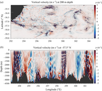
The motivation for the current study arises from realistic regional simulations of the SO that show large lee waves penetrating high into the water column and reflecting from the surface. Figure 1 shows vertical velocities from a recent nested simulation of the Drake Passage at  $0.01^{\circ }$ resolution, performed using the hydrostatic configuration of the Massachusetts Institute of Technology general circulation model (MITgcm, Marshall et al. Reference Marshall, Adcroft, Hill, Perelman and Heisey1997). For details of the model set-up see Mashayek et al. (Reference Mashayek, Ferrari, Merrifield, Ledwell, St Laurent and Naveira Garabato2017) – the model shown here has an improvement of vertical resolution from
 $100$ to
 $225$ vertical levels, with
 $10\ \textrm {m}$ resolution at the surface and
 $\leq 25\ \textrm {m}$ for all depths above
 $-4500\ \textrm {m}$, allowing better resolution of the energetic internal wave field. The vertical diffusivity and viscosity have background values of
 $5 \times 10^{-5}\ \textrm {m}^{2}\,\textrm {s}^{-1}$, and are enhanced by the
 $K$-profile parametrisation with the critical Richardson number for shear instability set to
 $Ri_c = 0.3$ (Large, McWilliams & Doney Reference Large, McWilliams and Doney1994). Biharmonic Leith horizontal viscosity is used with a coefficient of
 $2$ (Leith Reference Leith1996; Fox-Kemper & Menemenlis Reference Fox-Kemper and Menemenlis2008).
A daily average of vertical velocity  $(\textrm {m}\,\textrm {s}^{-1})$ in a realistic simulation of the Drake Passage showing a strong lee wave field throughout the water column (details in main text). (a) A plan view at
 $200\ \textrm {m}$, and (b) a vertical slice through the dashed line in (a).

Figure 1(a) shows a plan view of a typical daily average of vertical velocity at  $200\ \textrm {m}$ depth. Lee waves appear as disturbances in the vertical velocity with
 ${O}(0.1^{\circ }) \sim {O}(6\ \textrm {km})$ horizontal wavelength. Figure 1(b) shows the corresponding vertical velocity on a slice, with strong lee wave generation at the very rough bottom topography and propagation throughout the water column. The vertical velocities are near zero at the surface, with vertical phase lines and a modal structure in the vertical indicative of superposition of the wave field due to reflection at the surface.
This phenomenon has also been seen in other realistic simulations. de Marez et al. (Reference de Marez, Lahaye and Gula2020) examined the interaction of the Gulf Stream with the Charleston Bump in high resolution realistic simulations, with a focus on lee wave generation. They found that the lee waves have a surface signature, and showed qualitative agreement with sun glitter images from satellite observations. The simulation output was compared with (unbounded) linear theory, and differences noted near the surface, where surface reflection in the simulations caused a modal structure in the vertical velocity. Rosso et al. (Reference Rosso, Hogg, Kiss and Gayen2015) investigated topographic influence on surface submesoscales using a realistic  $1/80^{\circ }$ resolution model of the Indian sector of the SO, and noted surface peaks in vertical velocity (their figure 3). Lee waves reaching the surface were identified in the simulations and noted as a potential source for these increased vertical velocities, but not investigated further as the focus was on vertical velocities caused by surface submesoscales. They reasoned that enhanced near surface vertical velocities in their figure 4(d) are unlikely to be generated by a lee wave evident at depth, both because the near surface vertical velocities have a vertical phase line, indicating that it is decoupled from the tilted lee wave phase lines below, and the r.m.s. vertical velocity has a near surface maximum. However, we will show that vertical phase lines near the surface and a subsurface maximum in r.m.s. vertical velocity are expected properties of lee waves that interact with the surface. Bachman et al. (Reference Bachman, Taylor, Adams and Hosegood2017) simulated a similar region of the Drake Passage to that shown in figure 1(a) to investigate the surface submesoscale field and vertical velocities. They found regions of surface intensified r.m.s. vertical velocity, and suggested that submesoscale circulations may not account for all such vertical velocities, with lee waves a potential source. In any case, the separation of surface submesoscales and lee waves is not clear due to their similar horizontal scales, and it is possible that they interact as a result.
Although there is evidence for near-surface lee wave structures in the above modelling studies, observational evidence is more scarce. In the Gulf Stream, synthetic aperture radar and sun glitter images from satellites have been used to diagnose the presence of lee waves downstream of seamounts (Zheng et al. Reference Zheng, Holt, Li, Liu, Zhao, Yuan and Yang2012; de Marez et al. Reference de Marez, Lahaye and Gula2020), and strongly suggest interaction between bottom generated internal waves and the surface. In one of the few in situ observations of lee waves, Cusack et al. (Reference Cusack, Naveira Garabato, Smeed and Girton2017) found evidence of enhanced vertical velocities throughout the water column all the way to the top 500 m of the ocean above a ridge of 2500 m depth in the Drake Passage, suggesting interaction between the large wave generated at the ridge and the surface. However, the authors are not aware of any direct observational evidence in the SO for interaction between the bottom generated internal wave field and the surface.
A rigid lid upper boundary condition for the lee wave problem has been considered in the past, and the resonant properties of the solutions investigated (Bretherton Reference Bretherton1969; McIntyre Reference McIntyre1972; Baines Reference Baines1995). Dossmann et al. (Reference Dossmann, Shakespeare, Stewart and Hogg2020) recently performed experiments to quantify the generation of topographic waves from a background flow with both steady and oscillatory components, developing a corresponding linear theory including both a rigid lid upper boundary and a Rayleigh friction to allow weakly viscous effects. Although coupling of the wave generation from quasi-steady flows and tides is the focus of their study, the linear theory is similar to our study of the steady component. Here, we also consider non-uniform background flows.
The radiation of lee waves under a changing background flow has been extensively studied in the atmospheric context, with a focus on parametrising wave drag due to isolated obstacles (mountains) in atmospheric models (Teixeira Reference Teixeira2014, and references therein). Particularly relevant are studies of trapped lee waves, whereby sharp changes in background flow with height allow partial wave reflection and resonance (Scorer Reference Scorer1949; Gill Reference Gill1982; Teixeira et al. Reference Teixeira, Miranda, Argain and Valente2005; Teixeira, Argaiń & Miranda Reference Teixeira, Argaiń and Miranda2013), leading to high and low drag states, with clear parallels with the resonances found due to the upper boundary in the current study. In particular, Bretherton (Reference Bretherton1969) performed a comprehensive linear study including a rigid lid boundary condition similar to ours. However, a rigid lid condition in the atmosphere is not realistic, so efforts were generally made to improve the treatment of the upper boundary and reduce its impact (Teixeira Reference Teixeira2014). This study is intended to demonstrate simple properties of oceanic lee waves under changing background conditions typical of the ocean, with a particular focus on their structure in the upper ocean due to the boundary condition at the surface. Typically, atmospheric lee wave studies focus on drag. In the oceanic context, both lee wave drag and mixing are important, thus our focus is also somewhat different to the aforementioned atmospheric studies.
The structure of this paper is as follows. In § 2, we review and derive the linear lee wave theory with viscous and diffusive terms and discuss boundary conditions, energetics, time dependence, WKB solutions and complications associated with the bounded solution and non-uniform background fields including resonance and critical levels. In § 3, we present the numerical solver in a bounded and unbounded domain and describe the modelling set-up. We present results from the linear solver in § 4, and discuss conclusions in § 5.
2. Theoretical framework
Following Bell (Reference Bell1975), we start from the rotating, incompressible, Boussinesq equations with the inclusion of Laplacian viscosity  $\mathcal {A}$ and diffusivity
 $\mathcal {D}$
 \begin{gather} \boldsymbol{u}^{{{{\dagger}}}}_t + \boldsymbol{u}^{{{{\dagger}}}} \boldsymbol{\cdot} \boldsymbol{\nabla} \boldsymbol{u}^{{{{\dagger}}}} + \boldsymbol{f} \times \boldsymbol{u}^{{{{\dagger}}}} ={-}\rho_0^{{-}1}\boldsymbol{\nabla} p^{{{{\dagger}}}} + b^{{{{\dagger}}}}\boldsymbol{\hat{z}} + \mathcal{A}\nabla^{2} \boldsymbol{u}^{{{{\dagger}}}}, \end{gather}
 \begin{gather}b^{{{{\dagger}}}}_t + \boldsymbol{u}^{{{{\dagger}}}} \boldsymbol{\cdot} \boldsymbol{\nabla} b^{{{{\dagger}}}} = \mathcal{D} \nabla^{2} b^{{{{\dagger}}}}, \end{gather}
 \begin{gather}\boldsymbol{\nabla} \boldsymbol{\cdot} \boldsymbol{u}^{{{{\dagger}}}} = 0, \end{gather}
where  $\boldsymbol {u}^{{{\dagger}} } = (u^{{{\dagger}} },v^{{{\dagger}} },w^{{{\dagger}} })$ is the velocity,
 $\boldsymbol {f} = (0,0,f)$ is the Coriolis parameter,
 $p^{{{\dagger}} }$ is the pressure (with the linear hydrostatic pressure
 $-\rho _0 g (z-H)$ due to the constant reference density
 $\rho _0$ removed),
 $b^{{{\dagger}} } = -(\rho ^{{{\dagger}} } - \rho _0)g/\rho _0$ is the buoyancy,
 $\rho ^{{{\dagger}} }$ is the density, g is the acceleration due to gravity and
 ${{\dagger}}$ is used to denote total (background plus wave) fields.
2.1. Base state
We specify that the background velocity is in the  $x$-direction, and both background velocity and stratification are steady and vary only in the vertical. The background velocity is given by
 $(U(z),0,0)$, pressure by
 $\bar {p}(y,z)$ and buoyancy by
 $\bar {b}(y,z)$, with the bar notation indicating a background field. Assuming that the impact of perturbations on the mean flow is not leading order, from (2.1) it must satisfy both geostrophic and hydrostatic balance
 \begin{gather} -fU ={-}\rho_0^{{-}1}\bar{p}_y, \end{gather}
 \begin{gather}0 ={-}\rho_0^{{-}1}\bar{p}_z + \bar{b}. \end{gather}
Eliminating  $\bar {p}$ from (2.4)–(2.5) gives the thermal wind balance
 \begin{equation} -fU_z = \bar{b}_y. \end{equation}
Requiring that the stratification  $N^{2} = \bar {b}_z$ is a function of
 $z$ only, (2.6) gives that
 $fU_{zz} = 0$. We therefore only consider base states such that
 $fU_{zz} = 0$, but continue the derivation for general
 $U(z)$ for use when
 $f=0$. This ensures that although
 $\bar {p}$ and
 $\bar {b}$ are functions of
 $y$,
 $\bar {p}_y$ and
 $\bar {b}_y$ are not, and the problem remains effectively two-dimensional so that all coefficients of the linearised problem to be derived in § 2.3 are independent of
 $y$.
2.2. Energy loss
A representation of lee wave energy loss is crucial to understanding the structure of the lee wave field in the vertical. Lee wave energy must either be reabsorbed by the mean flow, or lost to dissipation and mixing. The latter is a result of energy transfer to smaller scales through instabilities of the waves themselves, or through nonlinear interactions with other waves and the background flow. In our idealised linear model, we cannot properly represent either the dynamics of the waves which can lead to instabilities and breaking, or small scales from other sources of turbulence that act to eventually dissipate even linear waves. The effect of this energy lost from the lee wave field must therefore be parametrised.
Parametrisation of dissipation and mixing at the sub-grid scale in models is generally implemented through Laplacian (or higher-order) viscous and diffusive terms in the momentum and buoyancy equations – as shown in (2.1)–(2.2). Shakespeare & Hogg (Reference Shakespeare and Hogg2017) provide a comprehensive overview of the role of Laplacian viscosity and diffusivity in the linear lee wave problem, with a focus on preventing excessive dissipation in wave resolving models. Here, we do not represent the processes that drain energy from the lee wave field, so aim to model them diffusively with this parametrisation. However, unlike Shakespeare & Hogg (Reference Shakespeare and Hogg2017), we are dealing with background flows that vary in the vertical, and thus including the vertical components  $\mathcal {A}_v\boldsymbol {u}_{zz}^{{{\dagger}} }$ and
 $\mathcal {D}_vb_{zz}^{{{\dagger}} }$ of the Laplacian terms in our study significantly complicates the solution.
For mathematical convenience, we therefore represent the total viscous and diffusive terms by the horizontal components only. This allows some scale selection for energy loss (improving on, say, a simple Rayleigh friction), without overly complicating the problem. Using only the horizontal component as a proxy for the total dissipation and mixing has certain drawbacks, including invalidating any solutions where the vertical wavelength changes drastically or becomes very small, e.g. at critical levels. It is important to keep in mind the simplifications made here when analysing the model mixing and dissipation in § 4. Direct comparisons between our horizontal turbulent viscosity  $\mathcal {A}_h$ and diffusivity
 $\mathcal {D}_h$ parameters and other studies or models should also be made with care, since they represent both horizontal and vertical viscosity and diffusivity. Furthermore, since
 $\mathcal {A}_h$ and
 $\mathcal {D}_h$ represent both background turbulent processes and breaking of the lee wave field itself, their ‘real’ values should depend on nonlinearity of the wave field and properties of the background flow, among other things. Although the simplifications made with this parametrisation are likely to modify our solutions somewhat, we believe that the key results of this study are unaffected.
2.3. Linearisation
For  $Fr_L \ll 1$, we consider small perturbations to the base state described in § 2.1. We consider a quasi-2-D flow such that the topography and waves are uniform in
 $y$. This choice is sufficient to demonstrate our main findings and greatly simplifies the problem, although the theory can be extended to 2-D topography without significant difficulties. The coefficients of the linearised equations are independent of
 $y$ due to the constraints on the base state described in § 2.1, thus the perturbation variables can be taken to be independent of
 $y$. We also assume here that the perturbations are steady, although this need not be imposed at this point and follows from the application of the steady boundary conditions to be described in § 2.4.
Letting  $\boldsymbol {u}^{{{\dagger}} } = (U(z) + u(x,z),v(x,z),w(x,z))$,
 $b^{{{\dagger}} } = \bar {b}(y,z) + b(x,z)$,
 $p^{{{\dagger}} } = \bar {p}(y,z) + p(x,z)$ and linearising (2.1)–(2.3) gives
 \begin{gather} wU_z + Uu_x -fv ={-}\rho_0^{{-}1}p_x + \mathcal{A}_h u_{xx}, \end{gather}
 \begin{gather}Uv_x + fu = \mathcal{A}_h v_{xx}, \end{gather}
 \begin{gather}\alpha Uw_x ={-}\rho_0^{{-}1}p_z + b + \alpha \mathcal{A}_h w_{xx}, \end{gather}
 \begin{gather}Ub_x - fvU_z +wN^{2} = \mathcal{D}_h b_{xx}, \end{gather}
 \begin{gather}u_{x} + w_{z} = 0, \end{gather}
where  $\alpha \in \{0,1\}$, so that when
 $\alpha = 0$ the equations are hydrostatic. The hydrostatic assumption is made when the ratio of vertical to horizontal scales is small, as is often the case for lee waves. We introduce a perturbation streamfunction
 $\psi$ such that
 $u = -\psi _z$,
 $w = \psi _x$, with Fourier transform
 $\hat {\psi }(k,z)$ defined such that
 \begin{equation} \psi(x,z) =\frac{1}{2{\rm \pi}} \int_{-\infty}^{\infty} \hat{\psi}(k,z)\textrm{e}^{\textrm{i}kx} \,\textrm{d}k . \end{equation}
Taking the Fourier transform in  $x$ of (2.7)–(2.11) and solving for the transformed streamfunction
 $\hat {\psi }(k,z)$ gives a second-order ordinary differential equation
 \begin{equation} \hat{\psi}_{zz} + P(k,z)\hat{\psi}_z + Q(k,z)\hat{\psi} = 0, \end{equation}
where
 \begin{gather} P(k,z) = \frac{f^{2}U_z\left(2U - \textrm{i}k(\mathcal{A}_h + \mathcal{D}_h)\right)}{\left(k^{2}(U - \textrm{i}k\mathcal{A}_h)^{2} - f^{2}\right)\left(U -\textrm{i}k\mathcal{A}_h\right)\left(U-\textrm{i}k\mathcal{D}_h\right)}, \end{gather}
 \begin{gather}Q(k,z) = \frac{k^{2}\left(U-\textrm{i}k\mathcal{A}_h\right)\left(N^{2} - \alpha k^{2}(U-\textrm{i}k\mathcal{A}_h)(U-\textrm{i}k\mathcal{D}_h)\right)}{\left(U - \textrm{i}k\mathcal{D}_h\right)\left(k^{2}(U-\textrm{i}k\mathcal{A}_h)^{2} - f^{2}\right)} - \frac{k^{2}U_{zz}(U-\textrm{i}k\mathcal{A}_h)}{k^{2}(U-\textrm{i}k\mathcal{A}_h)^{2} - f^{2}}. \end{gather}
With constant background velocity and stratification and in the absence of viscosity and diffusivity, this reduces to the familiar equation for the steady lee wave problem (Bell Reference Bell1975)
 \begin{equation} \hat{\psi}_{zz}(k,z) + k^{2}\frac{N^{2} - \alpha U^{2}k^{2}}{U^{2}k^{2} - f^{2}}\hat{\psi}(k,z) = 0, \end{equation}
with solution
 \begin{equation} \hat{\psi}(k,z) = A(k)\textrm{e}^{\textrm{i}m(k)z} + B(k)\textrm{e}^{-\textrm{i}m(k)z}, \end{equation}
for some functions  $A$ and
 $B$ to be specified by the boundary conditions, where
 \begin{equation} m^{2}(k) = k^{2}\frac{N^{2} - \alpha U^{2}k^{2}}{U^{2}k^{2} - f^{2}}. \end{equation}
It is clear from (2.17) and (2.18) that there are radiating solutions (lee waves) only when  $m$ is real, that is when the topographic wavelength
 $k$ satisfies
 \begin{equation} |\,f| < |Uk| < |N|. \end{equation}
For wavenumbers  $k$ in this radiating range, rotation can be neglected when
 $|\,f| \ll |Uk|$, and the hydrostatic assumption (
 $\alpha = 0$) can be made when
 $|Uk| \ll |N|$, since in this case the vertical wavenumber
 $m \sim {N}/{U}$ (from (2.18)), so
 $|Uk|/|N|$ represents the ratio of vertical to horizontal wavelengths.
2.4. Boundary conditions
2.4.1. Bottom boundary condition
For a given  $k$, (2.13) requires two boundary conditions. A free slip condition to ensure that the flow is parallel to the 2-D topography
 $h(x)$ is given by
 \begin{equation} w^{{{{\dagger}}}}(x,h) = u^{{{{\dagger}}}}(x,h)h_x. \end{equation}
Linearising about the base state then gives
 \begin{equation} w(x,0) = U(0)h_x, \end{equation}
or equivalently, defining the Fourier transform of the topography  $\hat {h}(k)$ similarly to (2.12)
 \begin{equation} \hat{\psi}(k,0) = U(0)\hat{h}(k). \end{equation}
Given this requirement, we write  $\hat {\psi }(k,z) = U(0)\hat {h}(k)\hat {\zeta }(k,z)$, where
 $\hat {\zeta }(k,z)$ is the normalised vertical structure function for a wavenumber
 $k$, so that
 \begin{equation} \psi(x,z) =\frac{U(0)}{2{\rm \pi}} \int_{-\infty}^{\infty} \hat{\zeta}(k,z)\hat{h}(k)\textrm{e}^{\textrm{i}kx}\, \textrm{d}k, \end{equation}
and  $\hat {\zeta }(k,z)$ satisfies
 \begin{gather} \hat{\zeta}_{zz} + P(k,z)\hat{\zeta}_z + Q(k,z)\hat{\zeta} = 0, \end{gather}
 \begin{gather}\hat{\zeta}(k,0) = 1. \end{gather}
2.4.2. Upper boundary condition
For the second condition, first consider the classical unbounded lee wave problem, which requires that waves propagate freely through the upper boundary. When the background flow is uniform in  $z$,
 $P$ vanishes,
 $Q$ is constant in
 $z$ and a vertical wavenumber
 $m(k) = \pm \sqrt {Q(k)}$ can be found. If the flow is also inviscid,
 $m(k)$ is given up to a sign by (2.18), and for the wave-like solutions with
 $k$ in the radiating range (2.19), there is then a well-defined vertical group velocity (to be discussed further in § 2.5). The vertical group velocity must be positive when the solutions are wave like so that energy radiates away from topography, and this is ensured by choosing
 $m(k)$ to have the same sign as
 $Uk$. When
 $m$ is imaginary (non-wave-like solutions), physical intuition necessitates that the positive root is taken so that disturbances decay away from topography rather than increase exponentially (see (2.17)).
If viscosity and diffusivity are non-zero, there is still a well-defined complex vertical wavenumber  $m(k) = \pm \sqrt {Q(k)}$. However, since
 $m$ is now complex, the correct choice for the sign of
 $m$ must always be that with positive imaginary part so that the solution decays away from the topography. Note that the previously non-radiating wavenumbers gain a small radiating component, although this is insignificant in the realistic limit of weak viscosity and diffusivity – see Shakespeare & Hogg (Reference Shakespeare and Hogg2017) for a detailed discussion. Here, we consider radiating lee waves from topography such that
 $|\,f| < |U(0)k| < |N(0)|$.
When the coefficients  $P$ and
 $Q$ are not constant in
 $z$, this radiating upper boundary condition is in general poorly defined, since for each
 $k$ there is not a well-defined vertical wavelength and group velocity. Waves can internally reflect and refract from changes in background density or velocity, so the solution cannot be restricted to upward propagating components. However, in some cases WKB solutions can be found for slowly varying background flows – see § 2.11.
If lee waves reach the upper ocean, the radiating upper boundary condition is inappropriate, and the air–sea interface may instead be better represented by a free surface boundary condition. A simpler condition is the rigid lid – we will show that for this problem, these are essentially equivalent.
At a free surface given by  $z = H + \eta (x)$, where
 $\eta \ll H$, the linearised kinematic boundary condition (cf. (2.21)) is
 \begin{equation} \psi(x,H) = U(H)\eta(x). \end{equation}
A further boundary condition is required to close the problem and is given by the dynamic condition that the pressure at the surface is equal to the atmospheric pressure  $p_A$ (assumed constant). The full pressure at the surface is
 $p^{{{\dagger}} }(x,z) = \bar {p}(z) + p(x,z)$, plus the linear term
 $-\rho _0 g (z-H)$ that was removed in the definition of
 $p^{{{\dagger}} }$ (see (2.1)). Expanding
 $p^{{{\dagger}} }(x,H + \eta (x))$ to first order in the perturbation variables and
 $\eta$, and using
 $\bar {p}(H)= p_A$, gives
 \begin{align} p^{{{{\dagger}}}}(x,H + \eta(x)) &\simeq p^{{{{\dagger}}}}(x,H) + \eta(x)\left.\frac{\partial {p^{{{{\dagger}}}}}}{\partial {z}}\right|_{z=H}, \end{align}
 \begin{align} &\simeq p_A + p(x,H) + \eta(x)\left.\frac{\partial {\bar{p}}}{\partial {z}}\right|_{z=H}. \end{align}
Invoking the boundary condition then gives
 \begin{equation} p_A = p_A + p(x,H) + \eta(x)\left.\frac{\partial {\bar{p}}}{\partial {z}}\right|_{z=H} - \rho_0 g \eta(x). \end{equation}
Using hydrostatic balance of the base state (2.5) then gives the dynamic boundary condition
 \begin{equation} p(x,H) = \rho_0 (g -\bar{b}(H))\eta(x) = \bar{\rho}(H)g\eta (x) = \rho_0 g \eta(x) , \end{equation}
where the reference density  $\rho _0$ is taken to be the base state surface density.
Eliminating the unknown  $\eta$ from the surface boundary conditions (2.26) and (2.30) gives the boundary condition
 \begin{equation} \psi(x,H) = \frac{U(H)p(x,H)}{\rho_0 g}. \end{equation}
This surface boundary condition could be used with the bottom boundary condition (2.21) to solve (2.7)–(2.11) , then the surface height recovered from (2.30) or (2.26). However, in practice this is unnecessary, as (2.31) can be well approximated by the rigid lid condition  $\psi (x,H) = 0$, equivalent to imposing
 $\eta (x) = 0$ (and thereby not satisfying the dynamic boundary condition). To see why, first notice from (2.7) that for negligible rotation, shear and viscosity,
 $p \sim -\rho _0 U u \sim \rho _0 U \psi _z$. For slowly varying background conditions, we expect
 $\psi (x,z)$ to locally have a sinusoidal structure in the vertical, so let (for fixed
 $x$)
 \begin{gather} \psi(z) \sim A\sin (mz + \theta), \end{gather}
 \begin{gather}\psi_z(z) \sim Am\cos (mz + \theta), \end{gather}
for some amplitude  $A$, wavenumber
 $m$ and phase
 $\theta$. Then, using the boundary relation (2.31):
 \begin{equation} \sin( mH + \theta) \sim \frac{mU^{2}}{g}\cos (mH + \theta). \end{equation}
Assuming that  $m \sim N/U$ (the hydrostatic, non-rotating limit of (2.18))
 \begin{equation} \tan (mH + \theta) \sim \frac{NU}{g} \ll 1, \end{equation}
even for large upper ocean values of  $U$ and
 $N$, and this scaling still holds for realistic conditions with rotation and non-hydrostatic waves. Therefore, the phase
 $\theta$ is such that
 $\psi (H) \simeq 0$, and it is clear that a rigid lid approximation is sufficient for determining the interior structure of the lee waves. The full free surface boundary condition could be implemented to determine exactly the (linear) surface height
 $\eta (x)$, but hereafter we only consider the rigid lid boundary condition. Since the interior flow is relatively unaffected by this approximation, we could still estimate the surface height without explicitly solving for it, using (2.30)
 \begin{equation} \eta(x) \sim \frac{p(x,H)}{\rho_0 g}, \end{equation}
where  $p(x,H)$ is found from the rigid lid solution.
With the rigid lid condition  $\psi (x,H) = 0$, the solution to the bounded problem is then given by (2.24)–(2.25), with the upper boundary condition
 \begin{equation} \hat{\zeta}(k,H) = 0. \end{equation}
2.5. Group velocities
The behaviour of lee waves in a bounded domain depends strongly on the direction of their group velocity. Consider the inviscid and unbounded problem with uniform background stratification and velocity, so that the vertical wavenumber  $m$ is independent of
 $z$. Re-deriving the governing equation (2.16) with time dependence by considering plane wave solutions
 ${\sim } \exp ({\textrm {i}(kx + mz -\omega t)})$ gives the dispersion relation (cf. (2.18))
 \begin{equation} (\omega - Uk)^{2} = \frac{N^{2}k^{2} + f^{2}m^{2}}{\alpha k^{2} + m^{2}}, \end{equation}
where  $\omega = 0$ for steady lee waves satisfying the boundary condition (2.21). The phase velocity is zero as a result, but the group velocity is non-zero and can be found by differentiating (2.38)
 \begin{align} \boldsymbol{c_g} &= \left(\frac{\partial {\omega}}{\partial {k}}, \frac{\partial {\omega}}{\partial {m}}\right), \end{align}
 \begin{align} &= \left( \frac{f^{2}(N^{2} - \alpha U^{2}k^{2}) + \alpha U^{2}k^{2}(U^{2}k^{2} - f^{2})}{Uk^{2}(N^{2} - \alpha f^{2})} , \frac{(U^{2}k^{2} - f^{2})^{3/2}(N^{2} - \alpha U^{2}k^{2})^{1/2}}{Uk^{2}(N^{2}-\alpha f^{2})}\right), \end{align}
where the sign of the vertical group velocity is taken to be positive when  $m$ is real, as is appropriate for the unbounded case, and it is assumed that
 $|\,f| < |Uk| < |N|$ so that the waves are radiating. It is clear from (2.40) that, in the non-rotating and hydrostatic case (
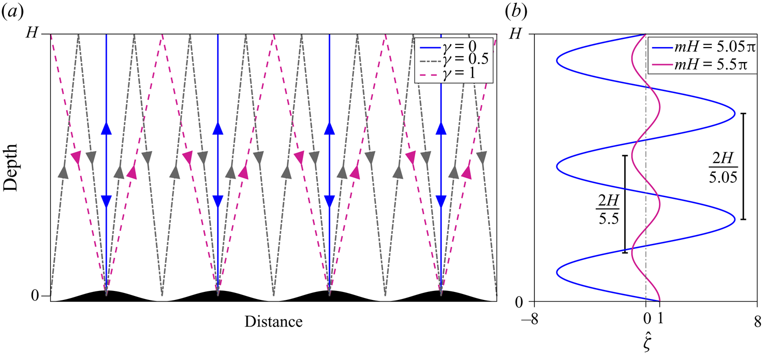
 $f = \alpha = 0$), the horizontal component of group velocity is zero, and waves propagate vertically upwards. Supposing now that they encounter the surface, the waves will reflect and propagate directly downwards – still with zero horizontal group velocity and now with negative vertical group velocity – superimposing exactly on the upward propagating wave field. This scenario is illustrated for monochromatic topography in figure 2(a) (blue lines). The reflected waves can then be expected to directly increase or decrease the topographic wave drag and energy conversion by constructive or destructive interference with the upwards propagating wave field at the topography. The extent to which this occurs is determined by the energy lost to mixing and dissipation during propagation, to be discussed in § 4.1. When the horizontal group velocity is zero, no energy propagates downstream, so without dissipative energy loss there can be no energy conversion into lee waves at the topography and also no wave drag (see § 2.8). However, there may be resonance (to be discussed in § 2.7).
(a) Diagram showing monochromatic topography with indicative ray paths for several values of the overlap parameter  $\gamma$, demonstrating some possible idealised paths of lee waves with different directions of group velocity. (b) Diagram showing the vertical structure function
 $\hat {\zeta }(k,z)$ for the analytic solution (2.42), for some vertical wavenumbers
 $m$ such that the solution is near resonant (blue) and at its minimum amplitude (magenta).

If  $|Uk|$ is of comparable magnitude to the Coriolis or buoyancy frequency, the waves will have a positive horizontal component of group velocity and will propagate both upwards and downstream, reflecting at the surface downstream of the topography. Without dissipation and mixing this could continue indefinitely and allow the lee wave energy to propagate far downstream, although in reality it seems unlikely that a significant amount of wave energy would undergo multiple reflections due to nonlinear interactions near the bottom boundary. For flow moving over the top
 $\sim U/N$ of an isolated topographic peak and generating a continuous range of wavenumbers
 $k$, if the angle of propagation (the angle of the group velocity vector to the vertical) is large enough for all radiating components, the reflected wave will not significantly interact with the generation process and the wave drag will be unchanged from the unbounded case. If the bump is not isolated, the reflected wave could be incident on the generation of a lee wave at a different topographic feature, and the drag (and energy flux) modification would be more complex.
To determine the likelihood of a lee wave superimposing on itself at the topography, we can determine the angle of propagation using (2.40), assuming for simplicity that  $U$ and
 $N$ are constant and viscosity and diffusivity are negligible. An ‘overlap parameter’
 $\gamma (k)$ can be defined as
 \begin{equation} \gamma (k) = \left|\frac{kH}{\rm \pi}\right|\tan \theta ,\quad \tan \theta = \left.\frac{\partial {\omega}}{\partial {k}} \right/ \frac{\partial {\omega}}{\partial {m}}, \end{equation}
where  $\theta$ is the angle of wave propagation to the vertical, and for each
 $k$,
 $\gamma$ is the horizontal distance travelled by a wave whilst propagating to the surface at
 $z=H$ and back to the topography at
 $z=0$, normalised by the horizontal wavelength. This is illustrated for
 $\gamma = 0, 0.5$, and
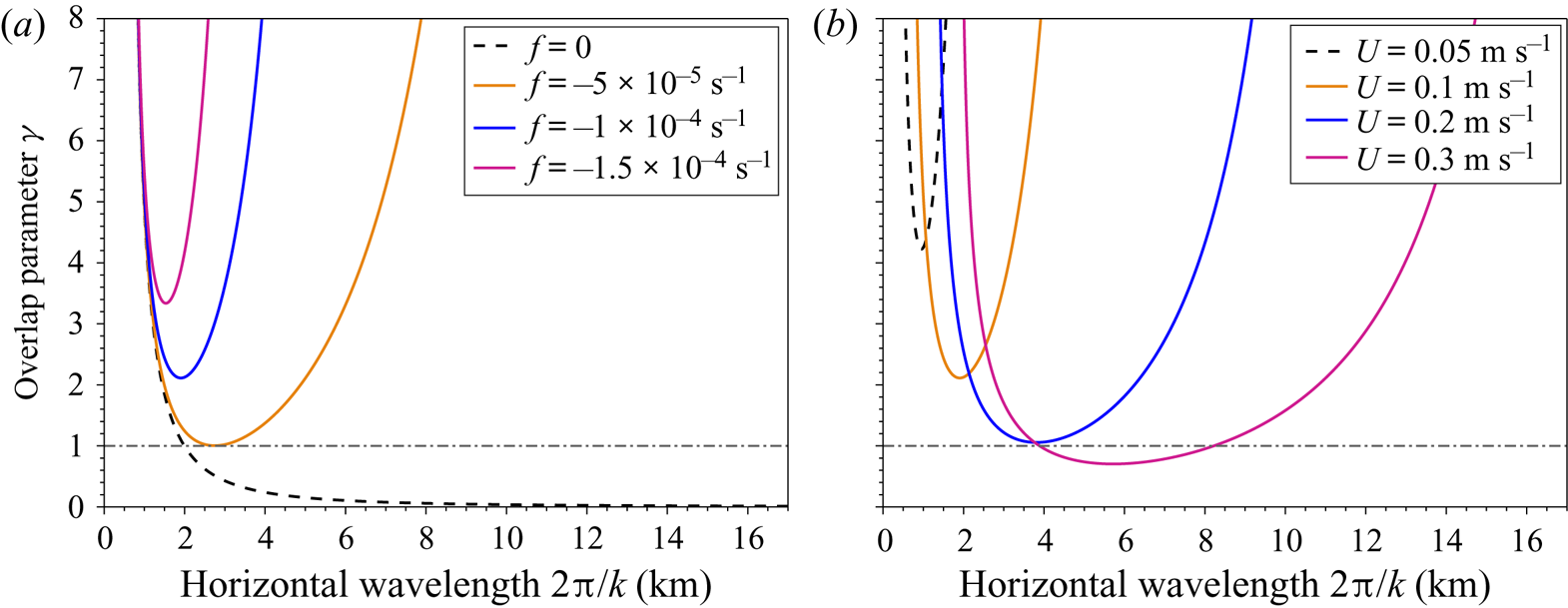
 $1$ in figure 2(a). Figure 3 shows the variation in
 $\gamma$ with horizontal wavelength
 $2{\rm \pi} /k$ for various
 $U$ and
 $f$. Each curve tends to infinity (not shown) at
 $k = |N/U|$ and
 $k = |\,f/U|$, at which point the vertical group velocity reaches zero and the solutions become evanescent. The increase in
 $\gamma$ for both large and small horizontal wavelengths is due to the increasing downstream component of group velocity.
Overlap parameter  $\gamma$ defined in (2.41a,b) for the non-hydrostatic case and (a) fixed
 $U = 0.1\ \textrm {m}\,\textrm {s}^{-1}$, varying
 $f$ and (b) fixed
 $f = -1\times 10^{-4}\ \textrm {s}^{-1}$, varying
 $U$, with
 $H = 3\ \textrm {km}$,
 $N = 1\times 10^{-3}\ \textrm {s}^{-1}$. The black dashed line shows
 $\gamma = 1$, below which a reflected lee wave could be expected to modify its own generation mechanism.

For smaller values of  $f$ (black dashed and orange lines in figure 3a) and larger values of
 $U$ (blue and magenta lines in figure 3b), there exists a range of scales at which
 $\gamma \lesssim 1$, indicating that reflected lee waves could impact on the generation mechanism by direct superposition. For
 $f = -1\times 10^{-4}\ \textrm {s}^{-1}$, characteristic of the SO, there exist horizontal scales at which this may be the case for
 $U \gtrsim 0.2\ \textrm {m}\,\textrm {s}^{-1}$. However, for
 $f = -1\times 10^{-4}\ \textrm {s}^{-1}$ and
 $U = 0.1\ \textrm {m}\,\textrm {s}^{-1}$ (orange line in figure 3b),
 $\gamma > 2$ for all radiating wavelengths, and all reflected waves return to topography at least
 $4\ \textrm {km}$ downstream of the generating topographic feature. Of course, this argument does not cover the more likely scenario of varying velocity and stratification with height. We conclude that for lee waves in shallow areas, low latitudes or high background flows it is possible for lee waves generated by isolated topography to reflect at the surface and modify the original wave drag and energy conversion, but that this is unlikely for deep generation, low background velocities and high latitudes.
When the topography is not isolated, and in particular when an artificially discrete topographic spectrum is used as in this study, the wave drag modification can be significant even when the overlap parameter is larger than one. For monochromatic topography, when  $\gamma (k) = n \in \mathbb {N}$, a wave generated at a topographic peak reflects at the surface and is incident on the topographic peak
 $n$ wavelengths downstream from the original, as shown in figure 2(a) for
 $n=1$, and impacts the wave field at that generation site in a similar way to the case
 $\gamma = 0$.
2.6. Analytic solution
When  $U$ and
 $N$ are constant with height, so that
 $P$ vanishes and
 $Q$ is a function of
 $k$ only, the solution to (2.24) for
 $\hat {\zeta }(k,z)$ is (extended from Baines Reference Baines1995)
 \begin{equation} \hat{\zeta}(k,z) = \frac{\sin(m(k)(H-z))}{\sin ( m(k)H )}, \end{equation}
where  $m(k)$ is the complex vertical wavenumber defined by
 $m^{2}(k) = Q(k)$, and the choice of sign does not matter. The solution can then be found numerically for general topography via (2.23), or analytically for monochromatic topography
 $h(x) = h_0\cos k_0 x$ to be
 \begin{equation} \psi(x,z) = Uh_0 \mathrm{Re} \left(\frac{\sin(m(k_0)(H-z))}{\sin ( m(k_0)H )}\textrm{e}^{\textrm{i}k_0 x}\right). \end{equation}
The above solutions are valid only when  $|m(k)H| \neq n{\rm \pi}$,
 $n \in \mathbb {N}$. At such points, resonances of the system occur.
2.7. Resonance
For uniform  $U$ and
 $N$, under the assumption that lee waves are hydrostatic (
 $|Uk| \ll |N|$), rotation is unimportant (
 $|Uk| \gg |\,f|$), and the system is inviscid, the vertical wavenumber is simply
 $m(k) = N/U$. The resonances of (2.42) are then independent of
 $k$, and occur when
 $|NH/U| = n{\rm \pi}$ for some
 $n \in \mathbb {N}$. There are no steady solutions to (2.24), (2.25) and (2.37) in this inviscid limit. Physically, this occurs when a whole number of half-wavelengths fits in the vertical domain and there is constructive interference of the upwards and downwards propagating waves. Figure 2(b) shows the vertical structure function
 $\hat {\zeta }$, defined in (2.42), for two real values of
 $m$. When
 $mH = 5.05{\rm \pi}$ (blue) the system is near resonance, as the half-wavelength nearly divides the depth
 $H$ (true resonance is at
 $mH = 5{\rm \pi}$). Thus,
 $\hat {\zeta }(z) = 0$ near
 $z=0$, so in order to satisfy the boundary condition
 $\hat {\zeta }(z=0) = 1$, the amplitude of the wave must be very large. At true resonance, this boundary condition cannot be met. In the opposite case, (shown for
 $mH = 5.5{\rm \pi}$ in magenta), there is destructive interference and the amplitude is at a minimum.
Under the above assumptions, the horizontal group velocity is zero, therefore energy cannot escape downstream and the wave generation at resonance continually reinforces the wave field. If this were to happen in practice, the wave amplitude would become large enough to invalidate the linearity of the wave field, perhaps causing nonlinear wave breaking or modifying the wave field or the boundary condition so as to move the system away from resonance.
When non-hydrostaticity is included, the horizontal group velocity is non-zero and the nature of the resonance changes slightly. The vertical wavenumber  $m(k) = \sqrt {N^{2}/U^{2} - k^{2}}$, thus the solution (2.42) has singularities at
 \begin{equation} k^{2} = \frac{N^{2}}{U^{2}} - \frac{n^{2}{\rm \pi}^{2}}{H^{2}}, \quad n \in \mathbb{N}\,. \end{equation}
Physically, these singularities still represent modes where an exact number of half vertical wavelengths fit in the domain, but now this happens at different values of  $U$,
 $N$ and
 $H$ for each component
 $k$ of the wave field.
Mathematically, the resulting singularities of (2.42) are simple poles, so when the topographic spectrum  $\hat {h}(k)$ is continuous (as for isolated topography), the integral (2.23) along the real line can be moved to a contour of integration in complex
 $k$ space that avoids the poles. To ensure that there is no disturbance at upstream infinity, the contour must be taken below rather than above the poles (McIntyre Reference McIntyre1972). The solution can then be expressed as the Cauchy principal value of (2.23) plus half the residues of the simple poles, which represent the non-hydrostatic resonant modes (Baines Reference Baines1995). The solutions, when
 $\hat {h}(k)$ is continuous, could be found numerically from (2.23) by choosing some contour of integration sufficiently far from the poles to avoid numerical difficulties. However, this becomes more difficult once rotation is included since the poles no longer all lie on the real axis. The numerical solution is also problematic since periodicity in the horizontal is assumed by default when taking a discretised Fourier transform, leading to spurious waves upstream of the isolated topography. If the topographic spectrum is discrete and includes one of the singular wavelengths defined by (2.44), then true resonance occurs and no steady solution exists.
The inclusion of energy loss through viscosity and diffusivity aids the numerical solution by moving all poles off of the real line so that the integral (2.23) can be found numerically with a simple fast Fourier transform (FFT). Although true resonance is avoided, states can still be near resonant, as will be shown in § 4.1. The topographic representation used here (see § 3.3) consists of a spectrum of topographic wavenumbers, which numerically becomes a sum of discrete components. This is likely to enhance the resonance effect compared with a more realistic and inhomogeneous topography.
2.8. Energy and momentum
The vertical linear lee wave energy flux at a given height is given by  $\overline {pw}$, where an overbar here represents a horizontal average. At the topography (
 $z=0$), this is equal to the product of the bottom mean flow velocity and the horizontally averaged form drag exerted by the topography on the mean flow, since using (2.21)
 \begin{equation} \overline{pw}|_{z=0} = U(0)\overline{ph_x}|_{z=0}. \end{equation}
Taking the inner product of (2.7)–(2.9) with the perturbation velocity and multiplying (2.10) by the perturbation buoyancy gives the energy equation for the wave field. Taking a horizontal average and assuming a periodic domain in the horizontal then gives an expression for the divergence of the energy flux
 \begin{equation} \overline{pw}_z ={-}\rho_0(U_zF + \bar{D}), \end{equation}
where  $\bar {D} = \overline {\varepsilon } + \bar {\varPhi }$ is the horizontally averaged energy loss from the flow, consisting of the dissipation rate
 $\varepsilon = \mathcal {A}_h|\boldsymbol {u}_x|^{2}$ and irreversible mixing
 $\varPhi = \mathcal {D}_hb_x^{2}/N^{2}$, and
 \begin{equation} F = \overline{uw} - \frac{f\overline{vb}}{N^{2}} \end{equation}
is the wave pseudomomentum flux, or the Eliassen–Palm (E–P) flux (Eliassen & Palm Reference Eliassen and Palm1960). If there are no critical levels ( $U \neq 0$) it can be shown from (2.7)–(2.10) that the E–P flux
 $F$ is related to the energy flux as (extended from Eliassen & Palm Reference Eliassen and Palm1960)
 \begin{align} \overline{pw} &={-}\rho_0U\left[ \overline{\left(u - u_x\mathcal{A}_h/U\right)w} - \frac{f}{N^{2}}\overline{\left(b - \mathcal{D}_hb_x/U\right)v}\right] \end{align}
 \begin{align} &={-}\rho_0UF\left(1 + {O}\left(\mathcal{A}_hk/U\right)\right), \end{align}
where  $k$ is the characteristic wavenumber of the topography, and
 $\mathcal {A}_h \sim \mathcal {D}_h$. Taking typical values considered here,
 $\mathcal {A}_h \sim 1\ \textrm {m}^{2}\,\textrm {s}^{-1}$,
 $k \sim 0.005\ \textrm {m}^{-1}$, and
 $U \sim 0.1\ \textrm {m}\,\textrm {s}^{-1}$, giving
 $\mathcal {A}_h k/U \sim 0.05 \ll 1$. Thus the energy flux is approximately equal to the local velocity multiplied by the E–P flux even when there is energy loss.
Since the source of the waves is at the bottom of the domain, the energy flux is always positive (or zero). (2.49) then gives that the E–P flux must have the opposite sign to  $U$, thus
 $F \leq 0$ in the cases considered here. This can be seen from the form of
 $F$ (2.47) in the non-rotating case, since a positive vertical velocity perturbation of the flow (
 $w > 0$) will correspond to the deceleration of a fluid parcel in the horizontal (
 $u < 0$), thus the momentum flux
 $\overline {uw} \leq 0$.
In the inviscid problem, (2.46) and (2.49) together give (Eliassen & Palm Reference Eliassen and Palm1960)
 \begin{equation} F_z =0. \end{equation}
Therefore, the E–P flux is conserved when there is no energy lost to dissipation and mixing. When there is also no vertical shear of the mean flow ( $U_z = 0$), (2.46) gives that the energy flux
 $\overline {pw}$ is also conserved. When the mean velocity increases or decreases with height, the energy flux increases or decreases correspondingly, but the E–P flux is still conserved. Any divergence of the E–P flux thus corresponds to the force exerted on the flow by the waves as they dissipate (Andrews & McIntyre Reference Andrews and McIntyre1976). It is the divergence of
 $F$ rather than the Reynolds stress (or momentum flux)
 $\overline {uw}$ that gives the relevant lee wave forcing on the mean flow, since
 $\overline {uw}$ is in general not conserved – a paradox explained by Bretherton (Reference Bretherton1969).
The total wave drag on the mean flow (defined here to be a positive quantity, although acting in the negative  $x$ direction) is therefore given by the integral of
 $\rho _0 F_z$ over the depth of the ocean. Since there cannot be any energy or momentum flux through the upper boundary,
 $\overline {pw}|_{z = H} = F(H) = 0$, thus the wave drag is given by
 $-\rho _0 F(0)$. Comparison of (2.45) and (2.49) then shows that up to
 ${O}(\mathcal {A}_h k/U)$ the wave drag is equal to the form drag.
Since  $\overline {pw}|_{z = H} = F(H) = 0$, if energy loss
 $\bar {D}$ is zero,
 $F = 0$ everywhere (from (2.50)) and
 $\overline {pw} = 0$ everywhere (from (2.49)), thus there is no net topographic wave drag on the flow or energy conversion to lee waves in steady state. This is true for a periodic domain – in a non-periodic domain the waves would propagate infinitely far downstream, and boundary fluxes would become important in the (2.46) and (2.49). Energy loss is therefore a key component of the bounded study, as there can be no topographic wave drag without it. This is a realisation of the ‘non-acceleration theorem’, first discussed by Charney & Drazin (Reference Charney and Drazin1961). Of course, in the unbounded problem there must also be energy loss in order to have wave drag at the topography – but that energy loss can implicitly occur by allowing the lee waves to exit the given domain (such that
 $\overline {pw}|_{z =H} > 0$) and dissipate ‘elsewhere’.
From (2.46), the wave energy flux can change both by exchange with a mean flow through the E–P flux (Kunze & Lien Reference Kunze and Lien2019), and by mixing and dissipation. Integrating (2.46) over the entire height of the domain gives
 \begin{equation} \overline{pw}|_{z=0} -\overline{pw}|_{z=H} = \rho_0\int_0^{H} U_zF + D\, \textrm{d}z. \end{equation}
If there is an upper boundary and no background shear ( $U_z = 0$), then
 $\overline {pw}|_{z=H} = 0$, and topographic energy conversion and wave drag are directly proportional to the total mixing and dissipation in the water column.
2.9. Time dependence
When calculating lee wave fluxes, it is usually assumed that the background fields and lee waves are steady. In reality, the geostrophic flows that generate lee waves vary on time scales of days to weeks. After a change in the background flow, the time taken for the lee wave field to equilibrate to the new steady state could be long compared with the typical time scales of the flow.
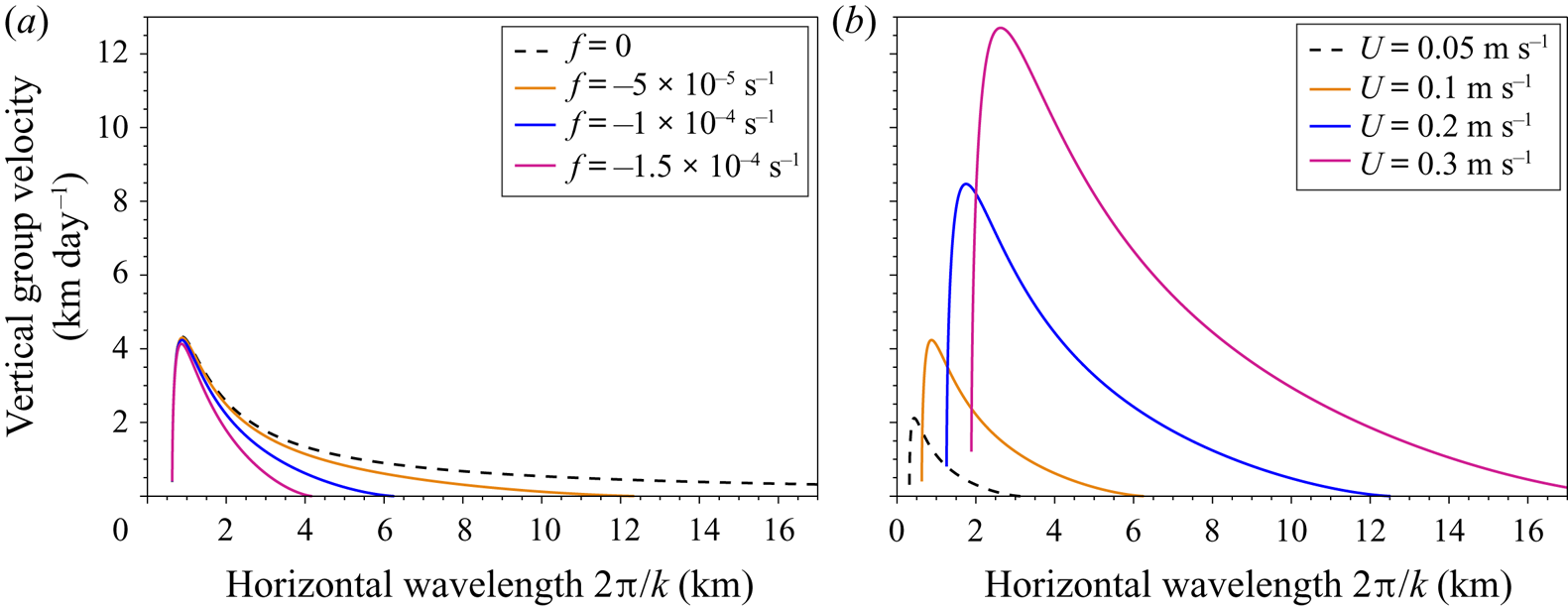
The relevant time scale in this study is the time taken for the lee wave to propagate from the topography to the surface. Figure 4 shows the vertical group velocity (defined in (2.40)) for various values of  $f$ and
 $U$. Lee waves generated at smaller horizontal scales (larger
 $k$) propagate faster, although they are also more likely to dissipate along the way due to sharper horizontal gradients. The effect of rotation on larger scales significantly slows the vertical group velocity, so that larger horizontal scale waves will take significantly longer to develop. The group velocity increases with
 $U$, so larger background velocities allow faster lee wave propagation. For a wave with wavelength
 $3\ \textrm {km}$ in a background flow
 $U = 0.1\ \textrm {m}\,\textrm {s}^{-1}$,
 $N = 1 \times 10^{-3}\ \textrm {s}^{-1}$ and
 $f = -1 \times 10^{-4}\ \textrm {s}^{-1}$, the vertical group velocity is approximately
 $1\ \textrm {km}$ per day, suggesting that a wave would take 3 days to propagate to the surface and a further 3 days to reflect back to the topography in an ocean of depth
 $3000\ \textrm {m}$. For a vertically varying background flow as is typical of the ocean, the vertical group velocity and wavelength will change during propagation, modifying this result. The time scale separation of full water-column lee wave formation and the mesoscale eddy field is therefore not clear, and depends on the scale of the waves. However, in energetic regions of the ocean such as the Drake Passage shown in figure 1, large velocities can enable high vertical group velocities and the steady approximation for lee waves at certain scales is expected to be valid.
Vertical group velocity defined in (2.40) for the non-hydrostatic case and (a) fixed  $U = 0.1\ \textrm {m}\,\textrm {s}^{-1}$, varying
 $f$ and (b) fixed
 $f = -1 \times 10^{-4}\ \textrm {s}^{-1}$, varying
 $U$, with
 $H = 3\ \textrm {km}$,
 $N = 1 \times 10^{-3}\ \textrm {s}^{-1}$.

2.10. Critical levels
In the inviscid and non-rotating problem, there are singularities of (2.13)–(2.15) at levels where  $U = 0$ (Booker & Bretherton Reference Booker and Bretherton1967; Maslowe Reference Maslowe1986). These are known as critical levels, where the horizontal phase speed of the wave (here equal to zero) equals the mean flow speed. At these levels, the vertical wavelength and group velocity vanish. No energy or momentum flux at the original wavenumber can propagate any further vertically, and the perturbation velocities become very large, invalidating the linear solution. In reality, instabilities and energy loss can lead to wave breaking and reflection at this level (Wurtele Reference Wurtele1996), thus critical levels may be a sink of lee wave energy in the ocean (Bell Reference Bell1975). However, this requires that the mean flow speed reaches zero somewhere in the water column. This is not a ubiquitous feature of the geostrophic eddies of the ACC, although critical levels may exist. This mechanism may be more important in regions of layered currents such as near the equator or in western boundary currents.
When rotation is included, there exist two further singularities of (2.13) at  $U= \pm |\,f/k|$, above and below the critical level
 $U = 0$ (Jones Reference Jones1967). These act to prevent the vertical propagation of the wavenumber
 $k$, in a similar way to the critical level of the non-rotating problem at
 $U = 0$. However, since each critical level is specific to the wavenumber
 $k$ (unlike for the non-rotating problem), if the spectrum of the topography is continuous it can be shown that there need not be singularities of the linear problem at these critical levels since the relevant solutions of (2.13) are logarithmic and thus integrable over a spectrum (Wurtele, Datta & Sharman Reference Wurtele, Datta and Sharman1996). Therefore, in reality there is not a single well-defined critical level for lee waves with rotation and a continuous spectrum of wavenumbers. However, the solutions may still become nonlinear so as to invalidate the linear solution and cause breaking. It can also be shown that when
 $f \neq 0$, the solution at
 $U = 0$ is no longer singular (Grimshaw Reference Grimshaw1975) – physically this is because all components have already reached their first critical level and stopped propagating.
When the flow is sheared such that  $|U|$ decreases with height, energy transfers from the lee waves to the mean flow via the E–P flux (see (2.46)), leaving less energy to be dissipated at the critical level for a particular wavenumber
 $k$. Kunze & Lien (Reference Kunze and Lien2019) examine this mechanism as a possible sink for lee wave energy in regions of intensified bottom flow. In particular, for lee wave energy generated at wavenumbers far from the inertial limit
 $|Uk| = |\,f|$, a greater proportion of the initial energy is available to be reabsorbed by a mean flow decreasing with height, allowing a smaller percentage to be dissipated at the critical level at
 $|Uk| = |\,f|$ or elsewhere. For waves generated close to the inertial limit (from large-scale topography), little energy is available for transfer to the mean flow, as it will instead soon reach its critical level and dissipate.
The inclusion of viscosity and diffusivity allows non-singular solutions to be found at critical levels where  $|Uk| = |\,f|$. However, near these levels the wave fields can become nonlinear, invalidating the linear approach. Furthermore, on the approach to these levels the vertical wavelength tends to zero, creating sharp vertical gradients and enhancing energy loss. Having neglected vertical viscosity and diffusivity in our solution, this energy loss does not take place. When the horizontal viscosity and diffusivity are large enough and shear small enough for the solutions to stay appropriately linear as a critical level is approached, the linear solution is valid, but may be unrealistic due to the lack of vertical dissipation and mixing. Velocity profiles that decrease with height are therefore not considered hereafter.
For positively sheared background flows where the flow speed increases with height, energy instead transfers from the mean flow to the lee waves during propagation (see (2.46)). Since wind driven oceanic currents tend to be surface intensified, this may be a common occurrence. In this case (or if stratification  $N$ decreases with height), the waves may reach ‘turning levels’, whereby their intrinsic frequency
 $|Uk|$ reaches the buoyancy frequency
 $N$ (Scorer Reference Scorer1949). At such levels the vertical wavenumber
 $m$ tends to zero (see (2.18)), and the wave is reflected downward. Scorer (Reference Scorer1949) showed that wave amplitudes in the resulting ‘trapped’ wave field could be increased by the superposition of reflected waves, much like in the current study due to the upper boundary. These turning levels are not the focus of our study, but may occur in the solutions for certain wavenumbers.
2.11. WKB solutions
Before solving the full equation (2.24) numerically, we first consider how much progress can be made with WKB theory (Gill Reference Gill1982). Under the assumption that waves are propagating through a slowly varying medium such that the wavelength is small compared with the scale of changes in the background flow, WKB theory can often be used to find closed form solutions. In addition to the necessary assumption for linear theory that there are no critical levels (where  $|U(z)k| = |\,f|$), WKB theory requires the further assumption that there are no turning levels (where
 $|U(z)k| = |N|$), since the vertical wavelength tends to infinity at these levels (see (2.18)). However, under the assumption that waves are generated and stay within the propagating range (2.19), solutions with both the rigid lid and freely radiating boundary condition can be found. For the latter, the component of the solution with positive local vertical group velocity is taken as in the uniform background case. de Marez et al. (Reference de Marez, Lahaye and Gula2020) find inviscid and non-rotating lee wave solutions under this approximation with a freely radiating boundary condition. Here, we extend their analysis to include rotation and viscous terms.
First, we write (for each  $k$)
 \begin{equation} \hat{\zeta}(z) = A(z)\textrm{e}^{\textrm{i}\varphi(z)}, \end{equation}
where  $A(z)$ and
 $\varphi (z)$ are some real amplitude and phase such that
 $\varphi '(z) \sim m \sim 1/\lambda _z$, where
 $\lambda _z$ is the vertical wavelength of the waves, itself varying over some length scale
 $L \gg \lambda _z$;
 $A(z)$ also varies on the length scale
 $L$ due to changes in the background flow and to viscosity. At this point we must therefore also take the weakly viscous approximation
 $\mathcal {A}_h^{2} k^{2}/U^{2} \ll 1$ to ensure that the decay scale due to viscosity is larger than the vertical wavelength of the waves (see (2.56) and discussion for justification). This is likely to be realistic in the ocean, as discussed after (2.49). Substituting (2.52) into (2.24), taking real and imaginary parts, and neglecting second-order terms in
 $\lambda _z /L$ allows two independent solutions to be found
 \begin{equation} \hat{\zeta}_\pm(k,z) = Q_r^{-{1}/{4}} \exp\left({\int_0^{z} -\tfrac{1}{2}(P_r \pm Q_i/\sqrt{Q_r}) \pm \textrm{i} \sqrt{Q_r} \, \textrm{d}\hat{z}}\right), \end{equation}
where  $\hat {z}$ is a dummy integration variable, and
 $Q_r, P_r$ and
 $Q_i, P_i$ are the real and imaginary parts of
 $P$ and
 $Q$, defined in (2.14) and (2.15). Setting
 $\mathcal {A}_h = \mathcal {D}_h$, and using the weakly viscous approximation, these become
 \begin{gather} Q_r = \frac{k^{2}(N^{2} - \alpha U^{2} k^{2} - U U_{zz})}{U^{2}k^{2} - f^{2}}, \quad Q_i = \frac{\mathcal{A}_h k^{3}\left[ 2Uk^{2}(N^{2} - \alpha f^{2}) - U_{zz}(U^{2}k^{2} + f^{2})\right]}{(U^{2}k^{2} - f^{2})^{2}}, \end{gather}
 \begin{gather} P_r = \frac{2f^{2}U_z}{U(U^{2}k^{2} - f^{2})}, \quad P_i = \frac{2\mathcal{A}_h f^{2} U_z k (3U^{2} k^{2} - f^{2})}{U^{2}(U^{2} k^{2} - f^{2})^{2}} . \end{gather}
Each term in (2.53) can be interpreted to understand the solutions;  $Q_r^{-{1}/{4}} \exp ({-\frac {1}{2}\int _0^{z} P_r\, \textrm {d}\hat {z}})$ determines the change in amplitude of solution due to changes in the background flow, and is constant in a uniform flow;
 $\exp ({\mp \frac {1}{2} \int _0^{z} Q_i/\sqrt {Q_r} \, d\hat {z}})$ determines how the wave amplitude exponentially decays (or ‘grows’, for a downwards propagating component) due to viscosity;
 $\exp ({\pm \textrm {i} \int _0^{z} \sqrt {Q_r} \, \textrm {d}\hat {z} })$ is the oscillatory component, with wavenumber
 $\sim \sqrt {Q_r}$ (cf. (2.17)).
The solution to the bounded problem can then be found using bottom and upper boundary conditions (2.25) and (2.37), and the solution to the unbounded problem can be found by taking  $\zeta _+(k,z)$ (see discussion in § 2.4.2) and using bottom boundary condition (2.25).
Simplifying further by considering the non-rotating and hydrostatic case with  $f = \alpha = 0$, and assuming a linear velocity profile with
 $U_{zz} = 0$, the WKB solutions are given by
 \begin{equation} \hat{\zeta}_\pm(k,z) = \sqrt{\frac{U}{N}} \exp\left({\pm \int_0^{z} \frac{N}{U}\left(\textrm{i} - \frac{\mathcal{A}_h k}{U}\right) \,\textrm{d}\hat{z}}\right). \end{equation}
Aside from reflections and viscous dissipation, we expect that as  $U$ and
 $N$ vary,
 $w \sim \hat {\zeta } \sim \sqrt {U/N}$,
 $u \sim \hat {\zeta }_z \sim \sqrt {N/U}$ and
 $\overline {uw} \sim \text {constant}$, as expected by conservation of the E–P flux (2.50). The length scale of viscous decay is given by
 $U^{2}/\mathcal {A}_h N k$, and the ratio of the vertical wavelength to the viscous decay scale is
 $\mathcal {A}_h k /U$, justifying the condition
 $\mathcal {A}_h^{2} k^{2} / U^{2} \ll 1$ for use of the weakly viscous approximation.
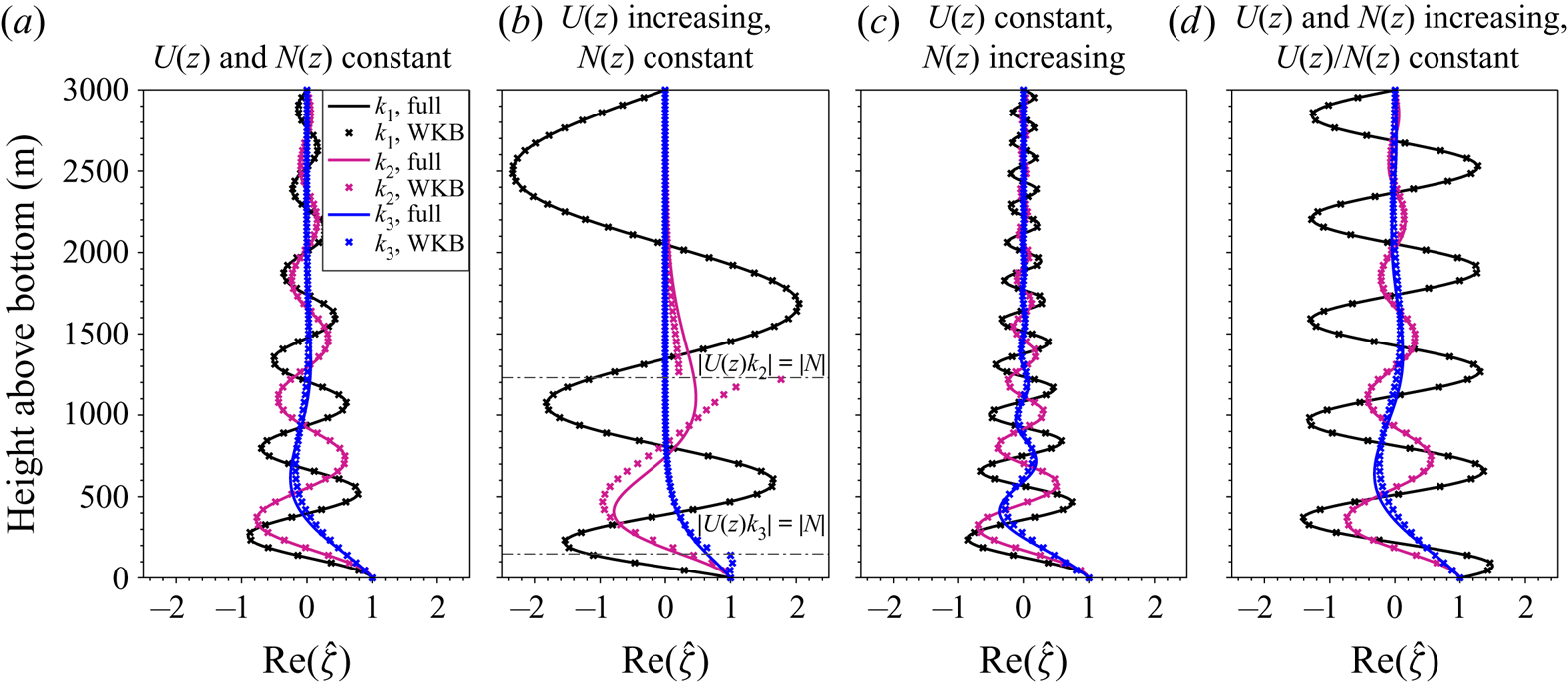
Figure 5 shows the WKB non-hydrostatic, rotating, bounded solution for  $\hat {\zeta }(k,z)$ and the corresponding full numerical solution (to be explained in § 3) for three different values of
 $k$ and various background profiles of
 $U(z)$ and
 $N(z)$. In figure 5(a,c,d) each of the wavenumbers
 $k_1, k_2, k_3$ remains within the propagating range (2.19) throughout the vertical domain, and the solutions are oscillatory. In each case, as
 $k$ increases, the amplitude of the solutions decreases, since the length scale of viscous decay decreases (cf. (2.56)). The exponential decay when
 $k=k_3$ (blue lines) is large enough that oscillatory component is small in comparison.
Numerical and WKB solutions  $\mathrm {Re} [\hat{\zeta}(k,z)]$ to the rotating, non-hydrostatic, bounded problem defined in (2.24), with boundary conditions (2.25) and (2.37). Background fields vary linearly from
 $U(0) = 0.1\ \textrm {m}\,\textrm {s}^{-1}$ and
 $N(0) = 1 \times 10^{-3}\ \textrm {s}^{-1}$; (a)
 $U(H) = U(0)$ and
 $N(H) = N(0)$, (b)
 $U(H) = 0.3\ \textrm {m}\,\textrm {s}^{-1}$ and
 $N(H) = N(0)$, (c)
 $U(H) = U(0)$ and
 $N(H) = 3 \times 10^{-3}\ \textrm {s}^{-1}$ and (d)
 $U(H) = 0.3\ \textrm {m}\,\textrm {s}^{-1}$ and
 $N(H) = 3 \times 10^{-3}\ \textrm {s}^{-1}$. Solutions are shown at
 $k = \{k_1 = k_{min} + 0.1(k_{max}-k_{min}), k_2 = 0.5*(k_{min} + k_{max}), k_3 = k_{max} - 0.1(k_{max} - k_{min})\}$, where
 $k_{min} = |f/U(0)|$,
 $k_{max} = |N(0)/U(0)|$, and
 $f = -1 \times 10^{-4}\ \textrm {s}^{-1}$.

In general, the numerical and WKB solutions agree well, although to a lesser extent as  $k$ increases since
 $m$ decreases (cf. (2.18)), and thus
 $\lambda _z$ increases, invalidating the WKB approximation. In figure 5(b)
 $U(z)$ increases and the solutions do not all stay within in the propagating range (2.19). Components
 $k_2$ and
 $k_3$ reach their turning levels where
 $|Uk| = |N|$, and the WKB approximation is not valid for these solutions.
Comparing the  $k=k_1$ component in figure 5(a) (constant background fields) with figures 5(b) (
 $U$ increasing) and 5(c) (
 $N$ increasing), we see that the scalings inferred from (2.53) hold, and the amplitude of
 $\hat {\zeta }$ (and
 $w$) increases with increasing
 $U$ and decreases with increasing
 $N$. The vertical wavelengths scale with
 $U/N$, although they are also dependent on
 $k$, as is expected from (2.18).
A further observation from figure 5(a,d) is the reduced impact of viscosity and larger amplitudes when  $U$ and
 $N$ increase together, even though
 $U/N$ is fixed. This is because the vertical group velocity of the waves is larger in this case – from (2.40) we can see that for
 $f^{2} \ll U^{2}k^{2} \ll N^{2}$, the vertical group velocity
 ${\sim } U^{2}k/N$. The waves have therefore decayed less by the time they reach and reflect from the surface. Equivalently, the decay scale due to viscous dissipation
 $U^{2}/\mathcal {A}_h N k$ increases with
 $U$ even when
 $U/N$ is fixed.
The WKB solutions are insightful provided there are no turning levels, and offer closed form solutions and insights that are not available from the numerical solutions. Similar approximations could also be made to implement a vertical and/or vertically variable viscosity, although we do not pursue this here to avoid further complexity. WKB solutions may therefore be more useful than numerical solutions in any eventual parametrisation of this process. However, hereafter we employ the full numerical solution, with no assumptions on the length scale of variations of the background flow or the viscous decay scale in order to study a wider range of wavenumbers and background flows.
3. Numerical solution
The full solution to the viscous linear lee wave problem will be found subject to both the radiating upper boundary condition (in which case we require  $U$ and
 $N$ to be constant with height, as discussed in § 2.4) and the rigid lid upper boundary condition, in which case we consider general
 $N^{2} > 0$ and
 $U(z)$ such that
 $U > 0$,
 $U_z > 0$ and
 $fU_{zz} = 0$ (see § 2.1).
3.1. Unbounded solver
The solution can be found in the traditional way (Bell Reference Bell1975), with the requirement the solution decays away from the topography as discussed in § 2.4. The solution for  $\psi$ is given by (2.23), where
 $\hat {\zeta }(k,z)$ satisfies (2.24)–(2.25), with the radiating upper boundary condition satisfied by taking the correct choice of branch for
 $m$. Note that
 $P(k,z) = 0$ and
 $Q(k,z) = Q(k)$, so the solution for
 $\hat {\zeta }$ is simply
 \begin{equation} \hat{\zeta}(k,z) = \textrm{e}^{\textrm{i}m(k)z}, \end{equation}
where  $m^{2}(k) = Q(k)$ and
 $\mathrm {Im}(m) > 0$. This can be implemented numerically for general topography 0
 $h(x)$ by performing the Fourier transforms with a FFT. Once
 $\psi$ is found, all other wave fields can be recovered.
3.2. Bounded solver
When the background flow is uniform in  $z$, the solutions can be found similarly to the unbounded case above, using the analytic solution (2.42) for
 $\hat {\zeta }(k,z)$. When
 $U$ and
 $N$ are not uniform, we use Galerkin methods to solve (2.24)–(2.37), an unforced second-order ordinary differential equation with inhomogeneous boundary conditions. First, we transform it into a forced problem with homogeneous boundary conditions. Let
 \begin{equation} \hat{\zeta}(k,z) = \hat{\phi}(k,z) + G(k,z), \end{equation}
where  $G$ is some function such that
 $G(k,0) = 1$ and
 $G(k,H) = 0$. Then
 $\hat {\phi }$ satisfies
 \begin{gather} \hat{\phi}_{zz} + P(k,z)\hat{\phi}_z + Q(k,z)\hat{\phi} = R(k,z), \end{gather}
 \begin{gather}\hat{\phi}(k,0) = 0, \end{gather}
 \begin{gather}\hat{\phi}(k,H) = 0 , \end{gather}
and  $R$ satisfies
 \begin{equation} G_{zz} + P(k,z)G_z + Q(k,z)G ={-} R(k,z). \end{equation}
 $G$ can be chosen to be any function satisfying
 $G(k,0) = 1$ and
 $G(k,H) = 0$. We choose it so that
 $R(k,0) = R(k,H) = 0$ by taking
 $G$ to be a cubic polynomial in
 $z$, and solving for the coefficients;
 $R$ can then be found via (3.6). The problem (3.3)–(3.5) can now be solved numerically using Galerkin methods. Specifically, for each
 $k$ we decompose
 $\hat {\phi }$,
 $P$,
 $Q$ and
 $R$ into finite Fourier sums with some truncation limit
 $M$
 \begin{equation} \left. \begin{aligned} \hat{\phi}(k,z) & = \sum_{s=1}^{M}a_s(k)\sin \frac{s{\rm \pi} z}{H}, \quad P(k,z) = \sum_{j=1}^{M}p_j(k)\sin \frac{(j-1){\rm \pi} z}{H}, \\ Q(k,z) & = \sum_{i=1}^{M}q_i(k)\cos \frac{(i-1){\rm \pi} z}{H}, \quad R(k,z) = \sum_{n=1}^{M}r_n(k)\sin \frac{(n-1){\rm \pi} z}{H} , \end{aligned} \right\} \end{equation}
where the  $q_i$,
 $p_j$ and
 $r_n$ are known and found via the relevant sine or cosine transform, and the coefficients
 $a_s$ are to be found. Notice that the sine expansion of
 $\hat {\phi }$ and
 $R$ ensures that their boundary conditions are satisfied. However, if
 $P \neq 0$ or
 $Q_z \neq 0$ at
 $z = 0,H$, the sine and cosine expansions of
 $P$ and
 $Q$ respectively must represent one or more discontinuities in
 $P$ or
 $Q_z$ at endpoints. The numerical solution is therefore an approximation that is valid only in the interior, although (3.3) is satisfied everywhere by the series expansions. There can also be noise at the frequency of the truncation limit near the endpoints of the series representations due to the Gibbs phenomenon. With increasing truncation limit and vertical resolution, the interior series solution approaches the actual solution at all interior points – (2.46) can be used to validate this. As a consequence, quantities should be evaluated with care at
 $z=0,H$, and (2.51) is used to find the wave drag rather than direct evaluation at
 $z=0$.
Substituting (3.7) into (3.3), integrating over  $z \in [0,H]$ and using the orthogonality properties of sine and cosine gives a matrix equation for the coefficients
 $a_s$
 \begin{equation} A_{sn}a_n = B_{sn}r_n, \end{equation}
where
 \begin{gather} A_{sn} ={-}\left(\frac{n{\rm \pi}}{H}\right)^{2}\delta_{s,n} \!+\! \frac{n{\rm \pi}}{2H}(p_{s-n+1} \!+\! p_{s+n+1} - p_{n-s+1}) + \frac{1}{2}(q_{s-n+1} + q_{n-s+1} - q_{s+n+1}), \end{gather}
 \begin{gather}B_{sn} = \delta_{n,s+1}. \end{gather}
The coefficients  $a_s$ can now be found from (3.8) by inverting the matrix
 $A$;
 $\hat {\phi }$ can then be recovered from the coefficients
 $a_s$,
 $\hat {\zeta }$ found from (3.2) and
 $\hat {\psi }$ found from (2.23).
3.3. Topography
The topography is found from the theoretical abyssal hill topographic spectrum proposed by Goff & Jordan (Reference Goff and Jordan1988), and is similar to that used in previous lee wave modelling studies (Nikurashin & Ferrari Reference Nikurashin and Ferrari2010a, Reference Nikurashin and Ferrari2011; Nikurashin et al. Reference Nikurashin, Ferrari, Grisouard and Polzin2014; Klymak Reference Klymak2018; Zheng & Nikurashin Reference Zheng and Nikurashin2019). This choice allows both comparison to the results of these studies, and consideration of the behaviour of a range of different wavenumbers without expanding the parameter space of investigation. The 1-D topography is found from the theoretical topographic spectrum  $P_{2D}(k,l)$
 \begin{equation} P_{2D}(k,l) = \frac{2{\rm \pi} h_0^{2} (\mu - 2)}{k_0 l_0}\left(1 + \frac{k^{2}}{k_0^{2}} + \frac{l^{2}}{l_0^{2}}\right)^{-({\mu}/{2})}, \end{equation}
by integrating over wavenumbers  $l$;
 $k_0$ and
 $l_0$ are the characteristic horizontal wavenumbers,
 $\mu$ is the high wavenumber spectral slope and
 $h_0$ is the r.m.s. abyssal hill height. For comparison with other recent lee wave studies, we set
 $k_0 = 2.3\times 10^{-4}\ \textrm {m}^{-1}$,
 $l_0 = 1.3\times 10^{-4}\ \textrm {m}^{-1}$ and
 $\mu = 3.5$, in line with representative parameters of the Drake Passage region used in Nikurashin & Ferrari (Reference Nikurashin and Ferrari2010b) and Zheng & Nikurashin (Reference Zheng and Nikurashin2019). Next,
 $P_{1D}(k)$ is set to zero for wavenumbers
 $k$ such that
 $|U(0)k| < |\,f|$ or
 $|U(0)k| > |N(0)|$, since solutions in these ranges are non-propagating. The typical values used are
 $N(0) =1\times 10^{-3}\ \textrm {s}^{-1}$,
 $U(0) = 0.1\ \textrm {m}\,\textrm {s}^{-1}$ and
 $f = -1\times 10^{-4}\ \textrm {s}^{-1}$, corresponding to a topography with wavelengths between
 $\sim 630\ \textrm {m}$ and
 $\sim 6300\ \textrm {m}$. Note that the same topography is used throughout, even when
 $f =0$.
The topographic height differs from that used in the aforementioned studies, since the solver is linear and the solutions must therefore remain approximately linear to be valid. We normalise the topography resulting from the above steps so that the r.m.s. of the final topography  $h_{rms} = 25\ \textrm {m}$. This gives a Froude number
 $Fr_L = Nh_{rms}/U = 0.25$ and is sufficient to keep the solution near linear such that the perturbation horizontal velocity
 $u$ is less than the background velocity
 $U$, with the exception of resonant cases. This is an unrealistically low Froude number for the rough topography of many parts of the SO (Nikurashin & Ferrari Reference Nikurashin and Ferrari2010b), but since the perturbation quantities are linear in
 $\hat {h}(k)$ (e.g. (2.23)), simple scaling arguments can recover the dependence on
 $h_{rms}$. The goal of this study is not to make predictions of the actual magnitude of the lee wave field, but its structure in the vertical and dependence on viscosity and diffusivity, background fields and boundary condition.
3.4. Numerical set-up
In the following section, the numerical solver is used to solve for the wave fields in a 2-D domain of width  $40\ \textrm {km}$, and height
 $3\ \textrm {km}$. The number of grid points in
 $x$ and
 $k$ is 800, and in
 $z$ is 257. The truncation limit
 $M$ (see (3.7)) is 200. Sensitivity tests were performed to ensure that increasing these resolutions does not impact the results.
The horizontal Prandtl number  $Pr_h = \mathcal {A}_h/\mathcal {D}_h$ is assumed to be equal to one throughout – Shakespeare & Hogg (Reference Shakespeare and Hogg2017) discuss the effect of non-zero Prandtl number on lee waves. Hereafter, we refer only to the viscosity
 $\mathcal {A}_h$, with the understanding that the diffusivity
 $\mathcal {D}_h$ varies similarly.
4. Results
Results from the numerical solvers are now presented. First, the hydrostatic and non-rotating solution is shown to demonstrate the resonance and modification of generation that occurs when the horizontal group velocity is zero, as described in §§ 2.5 and 2.7. Next, non-hydrostatic effects and rotation are introduced to the solution, and the results compared to the previous case. Finally, the effects of non-uniform stratification and velocity are shown.
4.1. Hydrostatic and non-rotating solutions
Figure 6(a,b) show the numerical linear solution for the vertical velocity field under the hydrostatic and non-rotating approximations with viscosity  $\mathcal {A}_h = 1\ \textrm {m}^{2}\,\textrm {s}^{-1}$. In figure 6(a), there is an open boundary (OB) and waves can freely propagate out of the domain, whereas in figure 6(b) the rigid lid (RL) boundary condition is implemented. The reflection of waves and superposition back onto the wave field is clear, as is the well-defined vertical wavenumber
 $m \sim N/U = 0.01\ \textrm {m}^{-1}$, giving a vertical wavelength of
 $2{\rm \pi} /m \sim 628\ \textrm {m}$. As discussed in § 2.5, when
 $f = \alpha = 0$, the horizontal component of group velocity is zero, as can be seen in the vertically radiating waves in figure 6(a,b). As a result, waves reflected at the surface superimpose directly back onto the original wave field. Notice that near topography the solutions in figure 6(a,b) are similar since energy has been lost in the reflected wave, thus the solution consists mostly of the original upwards propagating component. This is also somewhat visible in figure 6(c), which shows the difference between the bounded and unbounded solutions – the greatest differences are seen near the surface.
Vertical velocity ( $\textrm {m}\,\textrm {s}^{-1}$) from the linear solver (a) with an open boundary,
 $f =0$, hydrostatic, (b) with a rigid lid,
 $f =0$, hydrostatic, (c) the difference between (b) and (a), (d) with an open boundary,
 $f = -1\times 10^{-4}\ \textrm {s}^{-1}$, non-hydrostatic, (e) with a rigid lid,
 $f = -1\times 10^{-4}\ \textrm {s}^{-1}$, non-hydrostatic and (f) the difference between (e) and (d). Here,
 $\mathcal {A}_h = 1\ \textrm {m}^{2}\,\textrm {s}^{-1}$,
 $U = 0.1\ \textrm {m}\,\textrm {s}^{-1}$,
 $N =1\times 10^{-3}\ \textrm {s}^{-1}$ for all cases. Topography
 $h(x)$ is shown, although it is applied in the linear approximation at its mean value of
 $z = 0$.

Section 2.7 describes how resonance can occur when  $N^{2}H^{2}/U^{2}= n^{2}{\rm \pi} ^{2}$,
 $n \in \mathbb {N}$, in the inviscid, non-rotating, hydrostatic scenario. Figure 7 demonstrates this phenomenon with the given topography spectrum for varying viscosity
 $\mathcal {A}_h$. Figure 7(a) shows the lee wave energy flux at
 $z = 0, 1000\ \textrm {m}$, and
 $H$ for the OB and RL solutions with
 $H = 9.95{\rm \pi} U/N \simeq 3126\ \textrm {m}$ (constructive interference) and
 $H = 9.5{\rm \pi} U/N \simeq 2985\ \textrm {m}$ (destructive interference). For the OB solution the energy flux at
 $z=0$ is almost independent of viscosity – it is modified slightly by the local viscous term at
 $z=0$ (not shown hereafter), but not the viscosity elsewhere in the domain since energy can only radiate away from the topography. As viscosity increases, the energy flux at
 $z = 1000\ \textrm {m}$ and the surface decreases as more energy is lost during propagation. At
 $\mathcal {A}_h = 1\ \textrm {m}^{2}\,\textrm {s}^{-1}$, approximately
 $40\,\%$ of the wave energy dissipates in the bottom
 $1000\ \textrm {m}$.
(a) Horizontally averaged vertical energy flux at various heights for the OB and RL hydrostatic and non-rotating solvers, against horizontal viscosity  $\mathcal {A}_h$. (b) Horizontally averaged vertical energy flux at
 $z=0$ (proportional to wave drag) for several values of viscosity
 $\mathcal {A}_h$ against ocean depth
 $H$. Vertical dashed lines and triangles indicate the singularities
 $N^{2}H^{2}/U^{2} = n^{2}{\rm \pi} ^{2}$,
 $n = 8,9,10,11$. Other vertical lines indicate the values of
 $H$ shown in (a). In both panels
 $U = 0.1\ \textrm {m}\,\textrm {s}^{-1}$,
 $N = 1 \times 10^{-3}\ \textrm {s}^{-1}$,
 $f = 0$.

For the RL solver, the results are markedly different for the two different domain heights  $H$. In both cases, the energy flux is zero at
 $z=H$ due to the boundary condition, and zero when
 $\mathcal {A}_h = 0$, since there can be no steady state energy flux into lee waves without mixing and dissipation (see (2.51)). Equivalently, all upwards propagating energy flux is cancelled out by the reflected downwards component. However, for the near resonant case, when a small value of viscosity
 $\mathcal {A}_h = 0.25\ \textrm {m}^{2}\,\textrm {s}^{-1}$ is introduced the energy flux at the topography increases to over 2.5 times that with no upper boundary. Now that there is no longer exact cancellation of the energy flux, constructive interference of the wave field initially allows the energy flux to increase with increasing
 $\mathcal {A}_h$. As viscosity increases further, energy loss of the reflected wave reduces the constructive interference and the energy flux at
 $z=0$ decreases, approaching that of the unbounded solution until it no longer ‘knows about’ the boundary. The energy flux at
 $z=1000\ \textrm {m}$ follows a similar pattern, approaching the OB flux as
 $\mathcal {A}_h$ increases.
In contrast, the energy flux in the RL solution with  $H = 9.5{\rm \pi} U/N$ remains smaller than that in the OB solution throughout, since the effect of the boundary is to produce destructive interference with the original wave field. When the energy flux at
 $z=0$ from the solution with constructive interference peaks at
 $\mathcal {A}_h = 0.25\ \textrm {m}^{2}\,\textrm {s}^{-1}$, the energy flux from the solution with destructive interference is
 ${\sim }13$ times smaller.
Figure 7(b) demonstrates this constructive/destructive behaviour of the wave field as  $H$ varies. Again, the OB energy flux at
 $z=0$ is almost constant with changes in
 $\mathcal {A}_h$ and constant with changes in
 $H$. The RL energy flux at
 $z=0$ for
 $\mathcal {A}_h = 0$ is shown in black dashes, with the triangles and asymptotes indicating the singularities at
 $N^{2}H^{2}/U^{2}= n^{2}{\rm \pi} ^{2}$,
 $n = 8,9,10,11$. When
 $\mathcal {A}_h \neq 0$, the solutions become continuous with peaks at the singularities (constructive interference) and troughs half-way between (destructive interference). As
 $\mathcal {A}_h$ increases, the energy flux approaches the constant value of the OB solution. The values of
 $H$ in figure 7(a) are shown as vertical lines in figure 7(b).
The vertical structure of the energy flux, r.m.s. vertical velocity, energy loss and vertical gradient of the E–P flux are shown in figure 8 for the same cases described in figure 7 at  $\mathcal {A}_h = 1\ \textrm {m}^{2}\,\textrm {s}^{-1}$. Figure 8(a) again demonstrates the difference in energy fluxes with the boundary condition and height of domain. Figure 8(b) shows a periodic vertical structure in the r.m.s. vertical velocity
 $w_{rms}$ of the RL solutions that does not exist in the OB solution, due to the superposition of upwards and downwards propagating waves. This has the effect of enhancing the maximum
 $w_{rms}$ over a vertical wavelength, and decreasing the minimum, so that even in the destructive interference case where the energy flux in the RL solution is significantly smaller than the OB solution, the peak
 $w_{rms}$ is larger than that of the OB solution.
Horizontally averaged (a) energy flux (b) r.m.s. vertical velocity, (c) energy loss, (d) vertical gradient of the E–P flux as a function of  $z$ for the OB solver and the RL solver with constructive and destructive interference. Here,
 $\mathcal {A}_h = 1\ \textrm {m}^{2}\,\textrm {s}^{-1}$,
 $f = 0$,
 $U = 0.1\ \textrm {m}\,\textrm {s}^{-1}$,
 $N =1\times 10^{-3}\ \textrm {s}^{-1}$.

The energy loss  $\bar {D}$ (the sum of mixing and dissipation rate) is shown in figure 8(c). In the RL case the vertical phases of the waves are aligned due to the surface boundary condition, and the mixing and dissipation rate individually have a sinusoidal structure out of phase with each other (not shown). This is due to the energy distribution in the wave alternating between kinetic and potential over a vertical wavelength. There is over 2.5 times more energy loss in total when
 $H = 9.95{\rm \pi} U/N$ (constructive interference) compared with when
 $H = 9.5{\rm \pi} U/N$ (destructive interference). Comparing the OB and RL solutions for
 $H = 9.5{\rm \pi} U/N$, it can be seen that energy loss in the RL solution is enhanced near the surface, suggesting that the upper boundary moves the distribution of wave energy (and therefore energy loss) higher up in the water column.
The vertical gradient of the E–P flux is shown in figure 8(d), representing the force on the flow due to wave breaking. In the RL cases,  $F_z$ has a periodic structure in the vertical due to the wave interference, which would impact the feedback of the waves on the mean flow. The vertical integral of
 $F_z$ gives the total wave drag on the flow, hence the constructive interference produces a high drag state and the destructive interference a low drag state.
4.2. Non-hydrostatic and rotating solutions
When rotation ( $f \neq 0$) and non-hydrostatic (
 $\alpha = 1$ in (2.9)) effects are introduced, the resonance and interference effects described in § 4.1 are no longer as straightforward. As shown in § 2.5, the horizontal component of the group velocity is now positive, allowing wave energy to travel downstream. Figure 6(d,e) show the vertical velocity field for the same background flow conditions and topography as figure 6(a,b), but now with
 $f = -1\times 10^{-4}\ \textrm {s}^{-1}$ and
 $\alpha = 1$. Waves now propagate downstream as well as vertically, and the resulting structure in the RL solution (figure 6e) is not as simple. However, the characteristic vertical phase lines and modal structure of the disturbances just below the surface caused by superposition of the reflected waves remain.
Rotation reduces the generation of larger horizontal scale waves (e.g. figure 4a), and the dominant components of the wave field are therefore more easily dissipated than in the non-rotating solution shown in figure 6(a,b). The vertical group velocity is also reduced by rotation (figure 4a), so the waves radiate more slowly away from the topography and lose more energy before reaching the surface. The wave field in the lower part of the domain of figure 6(e) therefore resembles the OB solution in figure 6(d) more closely than in the non-rotating solution, since the dominant wavelengths have lost more energy by the time they return to the topography. The similarity of these two fields near the topography can be seen in figure 6(f), which shows the difference between figures 6(e) and 6(d).
Figure 9 shows the same data as figure 7, now with rotation and non-hydrostaticity included, for two domain heights  $H$ that have been picked to represent constructive and destructive interference of the new system. It is clear from figure 9(b) that the simple hydrostatic resonance has been replaced by multiple resonances where
 $|m(k)H| \simeq n{\rm \pi}$ (cf. (2.43)) for some
 $n \in \mathbb {N}$ and some
 $k$ in the spectrum
 $\hat {h}(k)$. As
 $H$ varies, the energy flux at the topography varies erratically as different wavenumbers
 $k$ in the topographic spectrum interfere constructively and destructively, with energy flux tending to that of the OB solution as
 $\mathcal {A}_h$ increases. The example values of
 $H$ in figure 9(a) are shown as vertical lines in figure 9(b). At
 $H = 3015\ \textrm {m}$ there is net destructive interference, and energy fluxes are below those of the OB solution, whereas at
 $H = 2982\ \textrm {m}$ there is net constructive interference, and the energy flux is higher than the OB solution. The RL solutions tend to the OB solutions with increasing
 $\mathcal {A}_h$ more quickly in figure 9(a) than in figure 7(a), since the dominant wavelengths are shorter and decay faster.
Same as figure 7, for the non-hydrostatic and rotating case with  $f =-1\times 10^{-4}\ \textrm {s}^{-1}$. Vertical lines in (b) indicate the values of
 $H$ shown in (a). Note that the domain heights
 $H$ picked to represent constructive and destructive interference of the system have changed.

Importantly, since the horizontal group velocities are now positive so that the reflected wave does not directly superimpose onto the upwards propagating wave, the main reason for the modification of the bottom energy flux (and wave drag) with a reflecting upper boundary is the periodic nature of the topography used. The overlap parameter (defined in (2.41a,b)) for this set of parameters is above 2 for all wavenumbers (orange line in figure 3b). If the topography were isolated, the bottom energy flux may not be changed at all, dependent on the relevant overlap parameter. Even when there are near resonances caused by constructive interference (peaks in figure 9b), they are smaller in amplitude than those in the hydrostatic, non-rotating case (figure 7b) since the waves are dispersive, and the resonances occur for individual wavenumbers rather than the whole wave field.
From figure 9(b), it is clear that, even with periodic topography, when  $\mathcal {A}_h \gtrsim 0.5\ \textrm {m}^{2}\,\textrm {s}^{-1}$, the constructive and destructive interferences with varying
 $H$ do not greatly affect the bottom energy flux; for
 $H > 3000\ \textrm {m}$ the change from the OB case is less than
 $10\,\%$. The value of
 $H$ is hereafter set to
 $3000\ \textrm {m}$, although shaded regions in figures 10, 12, 13, 14 and 16 show the range of solutions for
 $H$ between
 $2900\ \textrm {m}$ and
 $3100\ \textrm {m}$ (with axes scaled onto
 $[0,3000\ \textrm {m}]$), to indicate the extent of the interference. Figure 10 shows the vertical structure of the fields as in figure 8 for the non-hydrostatic and rotating RL and OB solutions at various values of
 $\mathcal {A}_h$. The profiles of energy flux in figure 10(a) show, as expected, that the RL solution approaches the OB solution as
 $\mathcal {A}_h$ increases. They will be identical when the energy flux at
 $z=H$ in the OB solution is zero.
Same as figure 8, for the non-hydrostatic and rotating case at various  $\mathcal {A}_h$. Results from the RL solver are shown as a range (shaded) of solutions with
 $H = 2900$ to
 $3100\ \textrm {m}$ (with axes scaled onto
 $z\in [0,3000\ \textrm {m}]$) to show the effect of constructive/destructive interference, and in solid for
 $H = 3000\ \textrm {m}$. Here,
 $f = -1\times 10^{-4}\ \textrm {s}^{-1}$,
 $U =0.1\ \textrm {m}\,\textrm {s}^{-1}$,
 $N = 1\times 10^{-3}\ \textrm {s}^{-1}$.

As was found in the hydrostatic and non-rotating case in figure 8(b), r.m.s. vertical velocity profiles shown in figure 10(b) are generally enhanced for the RL compared with the OB solution. The value of  $w_{rms}$ oscillates in
 $z$ due to the constructive and destructive interference of the wave field, with the maxima significantly larger than the OB solution, and the minima often larger too, especially in the lower viscosity cases. In particular, the subsurface maxima (located approximately
 ${\rm \pi} U/2N \simeq 157\ \textrm {m}$ below the surface) are significantly larger than the OB solution at that level, 1.8–1.9 times larger for each of the values of
 $\mathcal {A}_h$ shown here. They are also larger than the next deeper maximum below for each
 $\mathcal {A}_h$, and even larger than the r.m.s. vertical velocities down to
 $z = 700\ \textrm {m}$ for
 $\mathcal {A}_h = 0.5\ \textrm {m}^{2}\,\textrm {s}^{-1}$. The effect of the boundary is clearly to enhance the r.m.s. vertical velocity in the upper ocean.
The energy loss shown in figure 10(c) is larger in the RL case than in the OB case for each value of  $\mathcal {A}_h$. This is expected, since energy leaves the domain in the OB case, but must stay in the domain and be dissipated in the RL case. There is a subtlety in that in the RL case the bottom energy flux itself can be modified (see shading in figures 10a and 9b and discussion), however, the effect is not significant here. Consistent with the results of Zheng & Nikurashin (Reference Zheng and Nikurashin2019), we find that the total energy loss over the water column is increased from the OB case, although the difference is not large, between
 $1\,\%$ for
 $\mathcal {A}_h = 2\ \textrm {m}^{2}\,\textrm {s}^{-1}$ and
 $26\,\%$ for
 $\mathcal {A}_h = 0.5\ \textrm {m}^{2}\,\textrm {s}^{-1}$. Assuming that the energy flux at the topography is unchanged by reflections, since
 $U$ is uniform with height the total energy loss for each case in figure 10(c) must be the same (see (2.51)) – but the OB solutions must be integrated to an infinite height to get this result. The main result of note is the difference in the distribution of energy loss in the water column when a RL is introduced – it is skewed towards the surface, with an increase of
 $45\,\%$ for
 $\mathcal {A}_h = 2\ \textrm {m}^{2}\,\textrm {s}^{-1}$ and
 $70\,\%$ for
 $\mathcal {A}_h = 0.5\ \textrm {m}^{2}\,\textrm {s}^{-1}$ in the top
 $1000\ \textrm {m}$ compared with the OB case. Of course, these results are sensitive to the choice of ocean depth used, since in the limit
 $H \rightarrow \infty$ the RL and OB cases will be identical (excepting the perfectly inviscid case). For greater depths
 $H$, the differences reported in the top
 $1000\ \textrm {m}$ will be less pronounced.
The gradient of the E–P flux (figure 10d) has a similar structure to the energy loss (figure 10c). This is because  $U$ is constant with height, and neglecting the effect of the upper boundary, both wave energy flux (the gradient of which for
 $U$ constant is given by
 $\bar {D}$ from (2.46)) and the E–P flux (with gradient
 $F_z$) decrease only due to mixing and dissipation. Equivalently to noting as above that the total height integrated energy loss should be the same, the total wave drag on the flow, given by the integral of
 $F_z$, should also be the same for the cases shown, although when restricting to
 $z \in [0,3000\ \textrm {m}]$ the total wave drag in the RL solutions is larger than that of the OB solutions.
For idealised, nonlinear, 2-D OB simulations with a similar topographic spectrum and flow parameters, Nikurashin & Ferrari (Reference Nikurashin and Ferrari2010a) found that  $\sim 10\,\%$ of lee wave energy dissipated in the bottom
 $1\ \textrm {km}$ for
 $Fr_L = 0.2$, and
 $\sim 50\,\%$ for
 $Fr_L \geq 0.5$ (representative of the Drake Passage). From the black dot-dashed line in figure 9(a), these regimes would equate to
 $\mathcal {A}_h = 0.2\ \textrm {m}^{2}\,\textrm {s}^{-1}$ and
 $0.7\ \textrm {m}^{2}\,\textrm {s}^{-1}$, respectively, here. Of course, the change in implied turbulent viscosity between the two regimes is largely down to the nonlinearity and subsequent breaking for higher Froude number. This suggests that if a linear solution with a constant turbulent viscosity is to have any success in practice, it must be adjusted for the actual nonlinearity of the waves.
Comparing the energy loss (figure 10c) with the common parametrisation for the exponential vertical decay of lee wave energy dissipation (Nikurashin & Ferrari Reference Nikurashin and Ferrari2013; Melet et al. Reference Melet, Hallberg, Legg and Nikurashin2014), the decay scale for the OB solver (calculated as the height above bottom at which energy loss is equal to  $\textrm {e}^{-1}$ times its bottom value) is approximately
 $1700\ \textrm {m}$ for
 $\mathcal {A}_h = 0.5\ \textrm {m}^{2}\,\textrm {s}^{-1}$,
 $800\ \textrm {m}$ for
 $\mathcal {A}_h = 1\ \textrm {m}^{2}\,\textrm {s}^{-1}$, and
 $400\ \textrm {m}$ for
 $\mathcal {A}_h = 2\ \textrm {m}^{2}\,\textrm {s}^{-1}$. Proposed values of the lee wave decay scale (Nikurashin & Ferrari Reference Nikurashin and Ferrari2013) range between
 $300\ \textrm {m}$ and
 $1000\ \textrm {m}$. This together with the comparison of the energy flux to the nonlinear simulations of Nikurashin & Ferrari (Reference Nikurashin and Ferrari2010a) suggests that we are in the correct parameter space for
 $\mathcal {A}_h$, and therefore that the upper boundary could have an influence on the wave field. We hereafter show results for
 $\mathcal {A}_h = 0.5$ and
 $1\ \textrm {m}^{2}\,\textrm {s}^{-1}$.
4.3. Non-uniform velocity and stratification
In reality, the assumption that background flow is uniform with height is unlikely to be valid when considering lee wave propagation throughout the entire water column. We now consider the impact of varying  $U(z)$ and
 $N(z)$ on the lee wave field.
Unlike in the unbounded case, when solving the lee wave problem with a RL upper boundary it is straightforward to solve with arbitrary mean flow velocity and stratification. Some constraints do apply, and we only consider velocity profiles  $U(z) > 0$ such that
 $fU_{zz}(z) = 0$, so that the base state is effectively two-dimensional (see § 2.1), and
 $U'(z) > 0$, to avoid difficulties with critical levels (see § 2.10). Typical oceanic conditions are characterised by lower velocities at depth and larger velocities at the surface, so this scenario is realistic, although lee wave generation at locations of intensified bottom velocities may also be important (Kunze & Lien Reference Kunze and Lien2019). The only constraint on the stratification
 $N^{2}$ is that
 $N^{2} \geq 0$ so that the mean flow is statically stable.
First,  $U$ is varied linearly from
 $U(0) = 0.1\ \textrm {m}\,\textrm {s}^{-1}$ to
 $U(H) = 0.1, 0.2$ or
 $0.3\ \textrm {m}\,\textrm {s}^{-1}$ with
 $N = 1\times 10^{-3}\ \textrm {s}^{-1}$ and
 $\mathcal {A}_h = 0.5$ and
 $1\ \textrm {m}^{2}\,\textrm {s}^{-1}$. The vertical velocity fields when
 $U(H) = 0.1$ and
 $0.3\ \textrm {m}\,\textrm {s}^{-1}$ are shown in figure 11(a,b) respectively for
 $\mathcal {A}_h = 1\ \textrm {m}^{2}\,\textrm {s}^{-1}$. It is clear that increasing
 $U(H)$ has a large effect on the wave field, with vertical velocities increased throughout the domain and increased dominant vertical and horizontal wavelengths as
 $U(z)$ increases.
Vertical velocity ( $\textrm {m}\,\textrm {s}^{-1}$) in the RL solver, with linear
 $U(z)$ and
 $N(z)$ with bottom values
 $U(0) = 0.1\ \textrm {m}\,\textrm {s}^{-1}$,
 $N(0) = 1\times 10^{-3}\ \textrm {s}^{-1}$ and (a)
 $U(H) = 0.1\ \textrm {m}\,\textrm {s}^{-1}$,
 $N(H) = 1\times 10^{-3}\ \textrm {s}^{-1}$, (b)
 $U(H) = 0.3\ \textrm {m}\,\textrm {s}^{-1}$,
 $N(H) = 1\times 10^{-3}\ \textrm {s}^{-1}$, (c)
 $U(H) = 0.1\ \textrm {m}\,\textrm {s}^{-1}$,
 $N(H) = 3\times 10^{-3}\ \textrm {s}^{-1}$, (d)
 $U(H) = 0.3\ \textrm {m}\,\textrm {s}^{-1}$,
 $N(H) = 3\times 10^{-3}\ \textrm {s}^{-1}$. Here,
 $\mathcal {A}_h = 1\ \textrm {m}^{2}\,\textrm {s}^{-1}$,
 $\alpha = 1$, and
 $f = -1\times 10^{-4}\ \textrm {s}^{-1}$ in all cases. Topography
 $h(x)$ is shown, although it is applied in the linear approximation at its mean value of
 $z = 0$.

As before, waves are generated at the topography in the range  $|\,f| < |U(0)k| < |N|$. This range can be visualised in figure 3(b) as the range of wavelengths for which the overlap parameter
 $\gamma$ is finite for
 $U = 0.1\ \textrm {m}\,\textrm {s}^{-1}$ (orange line). These are the only propagating wavelengths that exist in the solution. However, as
 $U$ increases with height to
 $U(H) = 0.3\ \textrm {m}\,\textrm {s}^{-1}$, the range of wavenumbers that can propagate shifts to
 $|\,f| < |U(H)k| < |N|$, shown in figure 3(b) as the range for which
 $\gamma$ is finite for
 $U = 0.3\ \textrm {m}\,\textrm {s}^{-1}$ (magenta line). Thus, wavenumbers
 $k$ such that
 $|N|/|U(H)| < |k| < |N|/|U(0)|$ must reach their turning levels and reflect downwards before reaching the surface. The waves that reach the surface therefore have an increased minimum horizontal wavelength, as seen in figure 11(b), and decay more slowly as a result. Furthermore, the WKB solution (2.56) for waves that do not reach turning levels showed (in the hydrostatic and non-rotating limit) that the viscous decay scale
 ${\sim }U^{2}/\mathcal {A}_h N k$, thus as
 $U$ increases the effect of viscosity is felt less by the waves. Equivalently, the vertical group velocity of the waves increases with increasing
 $U$ (shown for uniform
 $U$ in figure 4b), leading to less energy loss during propagation over a given vertical distance. The reduced viscous decay results in increased interference between upwards and downwards propagating waves (cf. figure 9), shown in figure 12 as the shaded range becoming wider with both increasing
 $U(H)$ and decreasing
 $\mathcal {A}_h$.
Same fields as figure 8, with  $\mathcal {A}_h = 0.5\ \textrm {m}\,\textrm {s}^{-2}$ (a–d) and
 $\mathcal {A}_h = 1\ \textrm {m}\,\textrm {s}^{-2}$ (e–h). Solutions are for the non-hydrostatic and rotating case at various
 $U(H)$, where
 $U(z)$ is linear and
 $U(0) = 0.1\ \textrm {m}\,\textrm {s}^{-1}$. Shading as in figure 10,
 $f = -1\times 10^{-4}\ \textrm {s}^{-1}$,
 $N = 1\times 10^{-3}\ \textrm {s}^{-1}$.

The energy flux when  $\mathcal {A}_h = 0.5\ \textrm {m}^{2}\,\textrm {s}^{-1}$ (figure 12a) is highly dependent on the choice of depth
 $H$, and there is significant interference when
 $U(H) = 0.2$ and
 $0.3\ \textrm {m}\,\textrm {s}^{-1}$ (shown by the wide magenta and blue shaded areas). The bottom energy flux when
 $U(H) = 0.3\ \textrm {m}\,\textrm {s}^{-1}$ changes from 65 to 155 % of its OB value (black dashed line) as
 $H$ varies between 2900 and
 $3100\ \textrm {m}$, and this makes it difficult to compare the profiles of these solutions. However, the energy flux when
 $\mathcal {A}_h = 1\ \textrm {m}^{2}\,\textrm {s}^{-1}$ (figure 12e) at all levels is greater when
 $U(H) = 0.2$ and
 $0.3\ \textrm {m}\,\textrm {s}^{-1}$ than when
 $U$ is uniform, except for near the topography when there is significant destructive interference (blue shaded area). Aside from the ranges of the solutions (shaded), there is not a large difference between the energy fluxes in the cases
 $U(H) = 0.2$ and
 $0.3\ \textrm {m}\,\textrm {s}^{-1}$, likely due to the effect of certain larger wavenumbers reaching their turning levels at
 $|U(z)k| = |N|$ and reflecting before reaching the surface, decreasing upwards energy flux at higher levels. From (2.49) and (2.50), the energy flux
 $\overline {pw}$ is expected to increase with increasing
 $U(z)$ when there is no energy loss and the E–P flux is conserved. However, the RL solution constrains the energy flux to vanish at the surface, thus the convexity of the energy flux in
 $z$ will be determined by the balance between the gradient of the E–P flux due to energy loss and reflection, and the gradient of
 $U(z)$.
The most obvious result of increasing the velocity with height is the increase in the r.m.s. vertical velocity, shown in figure 12(b,f). Despite the large ranges due to interference, especially when  $\mathcal {A}_h = 0.5\ \textrm {m}^{2}\,\textrm {s}^{-1}$, increasing
 $U(H)$ clearly increases
 $w_{rms}$ over the whole water column. This is consistent with the expected scaling from the WKB solution (2.56) and figure 5(b). When
 $\mathcal {A}_h = 1\ \textrm {m}^{2}\,\textrm {s}^{-1}$ and
 $U(H) = 0.3\ \textrm {m}\,\textrm {s}^{-1}$ (figure 12f, blue line), the subsurface maximum is 4.5 times as large as that when
 $U(H) = 0.1\ \textrm {m}\,\textrm {s}^{-1}$ (black line), and over twice as large as its bottom value. The vertical wavelength also clearly increases with increasing
 $U$, as also seen in figure 11(b).
As discussed by Kunze & Lien (Reference Kunze and Lien2019), lee waves can exchange energy with the mean flow due to conservation of wave action  $E/kU$, where
 $E$ is the energy density (Bretherton & Garrett Reference Bretherton and Garrett1969). For a given wavenumber
 $k$, when there is no energy lost to dissipation, the wave energy density will therefore increase with height when
 $U$ increases with height. Here, the energy lost to dissipation means that the wave action is not conserved, but we still expect the wave energy to increase in the upper water column when
 $U(z)$ increases with height compared with when
 $U(z)$ is constant. Energy loss would also be expected to increase along with wave energy density for a given wavenumber. Similarly to the energy flux in figure 12(a), the large shaded areas in the energy loss in figure 12(c) due to interferences in the case
 $\mathcal {A}_h = 0.5\ \textrm {m}^{2}\,\textrm {s}^{-1}$ make interpretation difficult. However, figure 12(g) for
 $\mathcal {A}_h = 1\ \textrm {m}^{2}\,\textrm {s}^{-1}$ demonstrates that energy loss over the water column does generally increase with increasing
 $U(H)$. However, because energy at some wavenumbers no longer reaches the surface, having reached the corresponding turning level at
 $|U(z)k| = |N|$, the increase in wave energy (and energy loss) in the upper ocean is not as great for the multichromatic spectrum of waves as for a single component that reaches the surface. The waves that do reach the surface also experience less energy loss due to their larger horizontal scale.
Although the energy loss is generally greater when  $U$ increases with
 $z$, figure 12(d,h) show that the vertical gradient of the E–P flux is not, aside from the changes due to interference. Since
 $F$ is conserved when there is no mixing or dissipation, the flux does not increase due to interaction with the shear. Neglecting wave interference from surface reflections at the topography, the total wave drag
 $-\rho _0F(0)$ depends only on the local bottom fields, and thus remains constant with changes in
 $U$ with height. However, the total mixing and dissipation need not, since the waves can gain energy from the mean flow during propagation.
We now consider the effect of increasing the stratification  $N(z)$ on the lee waves in the RL solver. The vertical velocity field is shown in figure 11(c). The vertical wavelengths are clearly reduced as
 $N$ increases, since the vertical wavenumber
 $m \sim N/U$. The vertical velocities are also reduced higher in the water column when compared with figure 11(a). Figure 13 shows the horizontally averaged vertical profiles as in figure 12. It is immediately clear from the lack of shaded area that in the cases shown, constructive/destructive interference does not greatly affect the amplitude of the solutions, even for the lower value of
 $\mathcal {A}_h$, and to a decreasing extent for increasing
 $N(H)$. This is because the vertical group velocity (2.40) scales as
 $1/N$, so the waves slow down and lose more energy during their propagation and thus interact less. If vertical viscosity and diffusivity were implemented, the smaller vertical wavelengths associated with increased
 $N$ would dissipate even more quickly.
Same fields as figure 8, with  $\mathcal {A}_h = 0.5\ \textrm {m}\,\textrm {s}^{-2}$ (a–d) and
 $\mathcal {A}_h = 1\ \textrm {m}\,\textrm {s}^{-2}$ (e–h). Solutions are for the non-hydrostatic and rotating case at various
 $N(H)$, where
 $N(z)$ is linear and
 $N(0) = 1\times 10^{-3}\ \textrm {s}^{-1}$. Shading as in figure 10,
 $f = -1\times 10^{-4}\ \textrm {s}^{-1}$,
 $U = 0.1\ \textrm {m}\,\textrm {s}^{-1}$.

Figure 13(b,f) show that the effect of increasing  $N$ with height is to reduce the vertical velocities, in agreement with the WKB solution (2.56). This is because increasing
 $N$ when
 $U$ is fixed makes the waves more inertial (since the upper bound for the radiating wavenumber range
 $N/U$ is increased, while the lower bound
 $f/U$ is fixed). Since varying
 $N$ with height does not affect the energy flux in the same way as changing the velocity does (cf. (2.49)), the other results in figure 13 are easily interpreted. The increase in energy loss associated with reduced group velocity when
 $N$ is increasing causes a reduction in energy flux (figure 13(e), less clear in figure 13(a) due to interference), and a skewing of energy loss (figure 13c,g) and gradient of the E–P flux (figure 13d,h) towards the lower part of the domain. Note from (2.51) that the vertically integrated energy loss for a given
 $\mathcal {A}_h$ is constant with changing
 $N(H)$ (when
 $U(z)$ is constant), as is the total wave drag force on the flow, given by the integral of
 $F_z$.
Next, we present results for simultaneously varying  $U(z)$ and
 $N(z)$, keeping their ratio constant at
 $U(z) = 100\times N(z)$, so that the vertical wavelengths of the lee wave field are comparable to the uniform background case. This is a fairly realistic scenario for the ocean, where both
 $U$ and
 $N$ can be expected to increase with height above bottom. Figure 11(d) shows the vertical velocity field when both
 $U$ and
 $N$ triple between the bottom and the surface. The vertical wavelengths are comparable with figure 11(a) as expected, however, the vertical velocities are intensified, and there is more interference of the upwards and downwards propagating waves.
The energy flux with height is shown in figure 14(a,e) for  $\mathcal {A}_h = 0.5$ and
 $1\ \textrm {m}^{2}\,\textrm {s}^{-1}$ respectively. As in figure 12, the ranges associated with interference are wider for larger
 $U(H)$ and smaller
 $\mathcal {A}_h$. In general, upper ocean energy flux appears to increase with increasing
 $U(H)$ and
 $N(H)$, although this is not clear for
 $\mathcal {A}_h = 0.5\ \textrm {m}^{2}\,\textrm {s}^{-1}$ because of the significant interference. This is due to energy flux increasing when
 $U$ increases with height (see (2.46) and (2.50)), without the impact of turning levels as in figure 12, since
 $U/N$ remains constant. The gradient of the E–P flux (figure 14d,h), has a similar structure in the vertical for each case, with a greater range due to interference for larger
 $U(H)$ and smaller
 $\mathcal {A}_h$. The distribution of the forcing on the mean flow is therefore largely unchanged by increasing
 $U$ and
 $N$ with height.
Same fields as figure 8, with  $\mathcal {A}_h = 0.5\ \textrm {m}\,\textrm {s}^{-2}$ (a–d) and
 $\mathcal {A}_h = 1\ \textrm {m}\,\textrm {s}^{-2}$ (e–h). Solutions are for the non-hydrostatic and rotating case at various
 $U(H)$, where
 $U(H)$ is linear and
 $U(H) = 100N(H)$. Shading as in figure 10,
 $f = -1\times 10^{-4}\ \textrm {s}^{-1}$.

The upper ocean energy loss for  $\mathcal {A}_h = 1\ \textrm {m}^{2}\,\textrm {s}^{-1}$ (figure 14g) increases with increasing
 $U(H)$ and
 $N(H)$, which can be explained as before by conservation of wave action as
 $U$ increases, transferring energy to the wave field and increasing the wave energy density and hence energy loss. However, unlike the
 $U$ increasing case (figure 12c), the energy loss at most heights is now strictly increasing with
 $U(H)$, since the constant ratio of
 $U/N$ means that the range of radiating wavenumbers does not change with height, thus no wavenumber reaches a turning level. The result of this is that the energy loss in the upper ocean is significantly enhanced when
 $U$ and
 $N$ increase with height. The energy loss in the upper
 $1000\ \textrm {m}$ is three times larger when
 $U$ and
 $N$ approximately triple with height than when they are uniform throughout the water column (both with a RL and
 $H = 3000\ \textrm {m}$). For the lower viscosity value
 $\mathcal {A}_h = 0.5\ \textrm {m}^{2}\,\textrm {s}^{-1}$ (figure 14c), the wide shaded regions due to interference make this result less clear, but the constructive interference allows the energy loss in the upper
 $1000\ \textrm {m}$ for
 $U(H) = 0.3\ \textrm {m}\,\textrm {s}^{-1}$ to be up to
 $\sim 6$ times as large as in the OB case.
The change in energy loss with height for the various background flows with  $\mathcal {A}_h = 1\ \textrm {m}^{2}\,\textrm {s}^{-1}$ is also illustrated in figure 15. As we have seen, energy loss increases slightly with height with respect to the uniform fields when
 $U$ increases with height, and decreases when
 $N$ increases with height. The combination of increasing both
 $U$ and
 $N$, however, allows the waves to stay in their radiating range and gives the maximum upper ocean energy loss.
Energy loss  $D$ (
 $\textrm {m}^{2}\,\textrm {s}^{-3}$) in the RL solver, with the same mean flow and parameters described in figure 11.

Another interesting result is the large increase in r.m.s. vertical velocity with height when  $U$ and
 $N$ increase together (figure 14b,f), suggesting that the increase of
 $w_{rms}$ due to increasing
 $U$ is dominant over the decrease in
 $w_{rms}$ due to increasing
 $N$ (see figures 12b,f and 13b,f). This is consistent with the WKB solution (2.56) and figure 5(d), and as discussed in § 2.11 is because of reduced energy loss due to the increased viscous decay scale, or equivalently the increased vertical group velocity, compared with the uniform background case. The subsurface maximum of
 $w_{rms}$ when
 $U(H) = 0.3\ \textrm {m}\,\textrm {s}^{-1}$ and
 $\mathcal {A}_h = 1\ \textrm {m}^{2}\,\textrm {s}^{-1}$ is twice as large as that when
 $U(H) = 0.1\ \textrm {m}\,\textrm {s}^{-1}$, and nearly 4 times as large as
 $w_{rms}$ in the OB solution at the same height. The impact of the boundary is substantial, with the variation in
 $w_{rms}$ over a vertical wavelength due to superposition increasing with increasing
 $U(H)$ and
 $N(H)$.
Finally, we consider the effect of a more realistic stratification in the upper ocean. Typically, there exists a maximum of stratification at the thermocline, and a mixed layer at the surface where stratification is near zero. We use a simplified example stratification representative of the mean stratification in realistic Drake Passage simulations (which are themselves constrained by observed hydrographic information), having a maximum at around  $500\ \textrm {m}$ depth and decreasing to zero at the surface (Mashayek et al. Reference Mashayek, Ferrari, Merrifield, Ledwell, St Laurent and Naveira Garabato2017). In reality, the stratification can have a second sharp maximum below the thin surface mixed layer dependent on seasonality, but the deeper thermocline is a persistent feature. For comparison with the previous experiments,
 $N$ is linear (and
 $N^{2}$ quadratic) at depth, and modified using a
 $\tanh$ function to create the thermocline. Figure 16(a) shows the profiles of
 $N^{2}$ used,
 $U$ is linearly increasing from
 $U(0) = 0.1$ to
 $U(H) = 0.3\ \textrm {m}\,\textrm {s}^{-1}$, and
 $\mathcal {A}_h = 1\ \textrm {m}\,\textrm {s}^{-2}$. The effect of the drop in stratification at the surface, as might be expected from figure 13(b,f), is to further enhance the subsurface peak in r.m.s. vertical velocity (figure 16b). Although
 $w_{rms}$ increases, the buoyancy and horizontal velocity perturbations decrease with
 $N^{2}$ near the surface (not shown), leading to a decrease in total flow energy and energy loss (figure 16c). The combined effect of increasing velocity with height above bottom, the reflecting upper boundary, and a near surface decrease in stratification all act to increase the subsurface peak in r.m.s. vertical velocity.
(a) Stratification, (b) r.m.s. vertical velocity and (c) energy loss as a function of  $z$ for the RL solver. Here,
 $U$ is linear with
 $U(z) = 0.1(1 + 2z/H)$. The linear
 $N$ profile is
 $N(z) = 0.001(1 + 2z/H)$, and with the thermocline included is
 $N(z) = 0.001(1 + 2z/H)\sqrt {(1+\tanh (18-20z/H))/(1+\tanh (18))}$. Results from the RL solver are shown as a range (shaded) of solutions with
 $H = 2900$ to
 $3100\ \textrm {m}$ (with axes scaled onto
 $z \in [0,3000\ \textrm {m}]$) to show the effect of constructive/destructive interference, and in solid at for
 $H = 3000\ \textrm {m}$. Here,
 $\mathcal {A}_h = 1\ \textrm {m}^{2}\,\textrm {s}^{-1}$,
 $f = -1\times 10^{-4}\ \textrm {s}^{-1}$.

5. Conclusions
Lee waves generated by stratified geostrophic flow over topography play an important role in the buoyancy and momentum budgets of the ocean, causing diapycnal mixing and drag on the mean flow when they break. Occurring at the sub-grid scale of global models, they require parametrisation to represent their effect on the mean flow.
Linear theory with constant background velocity and stratification and a radiating upper boundary has often been used to predict the generation rate of lee waves. However, although this approximation may be sufficient locally to estimate the generation of lee waves, it does not allow any deductions on their propagation throughout the water column and eventual dissipation or re-absorption to the mean flow. The mean velocity and stratification in typical oceanic flows varies by up to an order of magnitude between the abyssal ocean and the surface, and the ocean surface is poorly represented by a radiating boundary condition, instead acting to reflect incident lee waves.
Motivated by high resolution realistic simulations of the Drake Passage, a region of high lee wave generation, we developed a theory for lee waves with an air–sea boundary, variable background velocity and stratification, and a representation of energy lost to dissipation and mixing. The structures observed in the simulations agree qualitatively with our theoretical predictions, and reconciling the two will be the subject of a follow up study.
We find that allowing lee waves to reflect at the surface has the potential to substantially modify the lee wave field, increasing vertical velocities and mixing and dissipation, especially in the upper ocean where shear and stratification are typically enhanced.
Allowing waves to reflect at the surface allows interference between the upwards and downwards propagating components, and this can modify the lee wave generation itself. Under certain conditions, this may manifest as a resonance of the system – although rotation and non-hydrostaticity act to lessen this effect.
The upper boundary alone acts to enhance near surface vertical velocities, and shift the energy loss of the lee wave field higher in the water column. However, the impact of our full water column view of lee waves is most significant when combined with non-uniform background flows, as are typical of realistic ocean conditions.
When the background velocity increases with height above the sea floor, as is often the case in wind driven geostrophic flows, we find that the impact of the reflection from the surface increases and that the lee wave vertical velocities are significantly enhanced in the upper ocean. The lee wave drag is largely unchanged, but the energy in the lee wave field, and hence the energy lost to mixing and dissipation, increases since energy transfers from the sheared mean flow to the waves. If the stratification also increases with height such that  $U/N$ remains fairly constant, the waves that are generated at topography are all able to reach the surface, increasing the upper ocean wave energy and energy loss. The inclusion of a weakly stratified surface mixed layer acts to enhance near surface vertical velocities further, and reduces near surface energy loss. Therefore, parametrising the effect of lee waves propagating through changing background flows may be essential for correctly estimating their impact on mixing.
The simplifications made in this study leave some questions as to the applicability of these results to the real ocean. In particular, although linear lee wave approximations have been shown to give good agreement with nonlinear simulations under certain conditions, the wave interactions discussed here that cause modification to wave drag and energy flux could be significantly altered by nonlinear topography. The assumption of linearity also has consequences for the wave–mean flow interaction, particularly when the background flow changes with height and energy transfers between waves and mean flow. Here, the mean flow is forced to remain constant, whereas in practice the mean flow would lose energy to the lee waves.
The contribution of time dependent components of the background flow, including tides, could change the nature of the wave generation and interactions. The coupling between internal tide and lee wave generation has recently been suggested to significantly affect lee wave generation rates, reducing global estimates of lee wave energy flux by 13 %–19 % (Dossmann et al. Reference Dossmann, Shakespeare, Stewart and Hogg2020; Shakespeare Reference Shakespeare2020). The unsteady nature of tides themselves could also impact the lee wave reflection and superposition through modification of the large-scale flow. Further studies are needed to quantify the impact of tidal flows on the mechanisms discussed here.
The constructive and destructive interference of the wave field may be overestimated due to the use of a periodic topography consisting of a finite sum of topographic components. It is likely that for a realistic topography, where the peaks of topography that generate lee waves are isolated and at different heights, this effect is substantially reduced. The effect of 3-D topography could also alter the results, and this could be investigated in the linear framework by extending the solver.
We implemented a horizontal viscosity and diffusivity in place of the full Laplacian parametrisation of lee wave energy loss for mathematical simplicity, which becomes unrealistic when the vertical scale of lee waves changes substantially over the depth of the water column. Breaking due to instabilities of the lee waves themselves is not explicitly accounted for, since the viscosity and diffusivity are constant with height. The appropriate values of viscosity and diffusivity should also vary with the nonlinearity of the waves themselves, and this could be especially important when the background flow changes with height, potentially changing the stability of the waves. The theory could be extended to allow a more realistic and vertically varying viscosity profile in a future work. However, using this simple parametrisation, the resulting energy loss can be tuned to agree with results from previous nonlinear simulations with similar topography and background flow (Nikurashin & Ferrari Reference Nikurashin and Ferrari2010a).
A rigid lid boundary condition has been used here, justified by the lack of impact of a free surface on the structure of the waves in the interior. However, predictions of the sea surface height imprint of these waves could be made within our theory. This could perhaps eventually allow observational diagnostics – modern satellite observations are fast approaching the  ${O}(1\ \textrm {km})$ horizontal resolution and
 ${O}(1\ \textrm {cm})$ precision that would be necessary to detect the very largest waves (Neeck et al. Reference Neeck, Lindstrom, Vaze and Fu2012). Satellite sun glitter images can also qualitatively be used to diagnose lee wave surface signatures (de Marez et al. Reference de Marez, Lahaye and Gula2020). The rigid lid condition would, however, be appropriate for modelling under-ice lee waves, whose surface normal stress could play a role in sea ice or ice shelf dynamics.
The results of this study indicate that the reflection of lee waves at the ocean surface and their presence in the upper ocean cannot always be neglected, especially when the mean flow is surface intensified. Climate model parametrisations may need to take into account the impact of changing background mean flows and surface reflections in order to correctly estimate the vertical structure of mixing and dissipation. Enhanced upper ocean mixing could have important consequences for tracer transport between the surface and interior ocean. The dynamics of the near surface wave field and its interaction with surface submesoscales should also be investigated further, since the horizontal length scales are very similar. Further studies will aim to verify the theory developed here against realistic nonlinear simulations, and investigate the impact of these waves on surface processes.
Acknowledgements
The authors are grateful to C. Shakespeare and two other anonymous reviewers of the manuscript for their helpful and constructive comments. All codes used in this paper are publicly available on GitHub at https://github.com/loisbaker/lee-wave-solver.
Funding
L.B. was supported by the Centre for Doctoral Training in Mathematics of Planet Earth, UK EPSRC funded (grant no. EP/L016613/1), and A.M. acknowledges funding from the NERC IRF fellowship grant NE/P018319/1.
Declaration of interests
The authors report no conflict of interest.