1 Introduction
Many studies have been reported in recent years that attempt to understand fluid dynamical problems that involve a fluid interface between two immiscible fluids. A first step is to characterize and measure the interface properties. A clean interface, free of the surface active agents (amphiphilic molecules or colloidal particles that are energetically attracted to the interface), is generally believed to be characterized solely by the static equilibrium surface free energy per unit area (i.e. the interfacial tension) and there are many successful ways to measure this quantity. The interfacial tension of a clean interface is a material property. Its value depends only on the thermodynamic state. Its influence on flow is due to the fact that changes in the shape of the interface that lead to an increase in interface area are resisted because they would increase the free energy. On the other hand, when surface active agents (surfactants) are present, the interfacial tension is reduced by an amount that depends on the local surfactant concentration (Levich Reference Levich1962). Surfactants may also give rise to a surface-excess rheology when compared with a clean interface (Edwards, Brenner & Wasan Reference Edwards, Brenner and Wasan1991; Slattery, Sagis & Oh Reference Slattery, Sagis and Oh2006). The influence of surfactants on flow is due then to two distinct effects. First, surfactant concentration gradients are often naturally produced by flows, which give rise to Marangoni stresses that impact the fluid dynamics of the system, independent of the surfactant’s surface rheology (and, in fact, even in the absence of surface rheology). Second, the surface-excess rheology will play a direct role in the motions within the interface and thus also in the contiguous bulk fluids. The importance of Marangoni effects depends on the sensitivity of the interfacial tension to surface concentration, and also on the rate at which concentration gradients are relaxed by interface diffusion and by adsorption/desorption of surfactant into the subphase region relative to the rate at which convection processes produce surfactant concentration gradients. However, in spite of these complexities, it is fair to say that Marangoni effects are well understood and extensively studied in the fluid mechanics literature.
By comparison, the understanding of interface rheology effects is far less well developed or understood. A major, generally unresolved, problem is the development of methods to measure the mechanical/rheological properties of interfaces. Not only is it difficult to determine whether the rheology is a simple Newtonian form or some more complex behaviour, but even in the former case, unambiguous methods to measure the interface viscosities are lacking in spite of the fact that this has been the focus of a variety of studies (Edwards et al.
Reference Edwards, Brenner and Wasan1991; Fuller & Vermant Reference Fuller and Vermant2012). Of particular concern is the fact that measurements of material properties of the interface, such as surface shear viscosity, often have reported values that are orders of magnitude apart (Stevenson Reference Stevenson2005). A possible culprit is that many methods generate a mixed interfacial flow, with both dilatation and shear components. Just as the shear and compressional moduli of solids cannot be determined from a single mixed-type deformation alone, the surface shear and dilatational viscosities cannot be unambiguously determined from measurements of a single mixed-type flow. One resolution to this issue, following practices developed in rheology, is to probe the interface in a way that produces a pure shear deformation. In fact, recent experimental studies using a rotating microdisk at an interface (Zell et al.
Reference Zell, Nowbahar, Mansard, Leal, Deshmukh, Mecca, Tucker and Squires2014) show that this device produces a pure shear flow, and does not generate surfactant gradients that might otherwise complicate the interpretation via the presence of Marangoni contributions to the torque. Measurements with the soluble surfactant SDS showed that it has a surface viscosity that is immeasurably small (corresponding to
 ${\it\eta}_{s}\lesssim 10^{-8}~\text{N}~\text{s}~\text{m}^{-1}$
) with
 ${\approx}10~{\rm\mu}\text{m}$
probes, even though other protocols reported values
 $10^{3}{-}10^{4}$
times higher (Zell et al.
Reference Zell, Nowbahar, Mansard, Leal, Deshmukh, Mecca, Tucker and Squires2014).
In spite of the apparent success of the rotating disk for measuring shear properties of an interface, an obvious question is whether other properties, such as those associated with dilatational flows, can be measured. For this purpose, the dynamics of a cylindrical probe that generates a mixed flow, containing elements of both shear and dilatation, may still appear as a viable possibility, or for that matter any probe that generates a flow that has a dilatational component (Cicuta & Terentjev Reference Cicuta and Terentjev2005; Verwijlen, Moldenaers & Vermant Reference Verwijlen, Moldenaers and Vermant2013). The basic question is whether the flows will also generate Marangoni contributions to the stress under flow conditions that are strong enough to probe the rheological properties, and, if so, whether the contributions of these stresses to the force (or torque) on the probe can be distinguished from the contributions of stresses associated with the surface-excess rheology. It is difficult to answer this question without a detailed theoretical study.
In the present work, we examine the resistance of a disk-shaped probe translating through a viscous interface laden with a soluble surfactant, including surface shear and dilatational rheology, Marangoni stresses and finite surfactant adsorption/desorption kinetics. Others have considered the consequence of a viscous compressible interface (Danov et al. Reference Danov, Aust, Durst and Lange1995; Barentin et al. Reference Barentin, Ybert, Di Meglio and Joanny1999; Dimova et al. Reference Dimova, Danov, Pouligny and Ivanov2000), but no work yet considers a probe at a viscous, compressible interface that generates Marangoni flows. Our work extends the analysis of Barentin et al. (Reference Barentin, Ybert, Di Meglio and Joanny1999), who considered a compressible Gibbs monolayer that equilibrates instantaneously with the subphase surfactant. Here we consider a finite ratio of the adsorption/desorption to convective time scales and as such consider the effects of small non-uniformities in the surfactant concentration field at the interface. We solve for the Marangoni flows that ensue due to surface tension variations and determine the resulting additional force on the probe. Dimova et al. (Reference Dimova, Danov, Pouligny and Ivanov2000) also considered concentration variations, but did not couple the interface to a bulk fluid and did not determine the Marangoni flow, but only the leading-order change in the surface tension. For analytical ease, as in Barentin et al. (Reference Barentin, Ybert, Di Meglio and Joanny1999), we assume a flat (two-dimensional) disk at the interface and solve the hydrodynamic equations explicitly assuming that the subphase is shallow compared to the radius of the disk. In this case, the bulk phase flow problem is reduced to the thin-film/lubrication limit and is effectively slaved to the interfacial dynamics. As a practical matter, the thin-film limit is not desirable for experimental studies of surface rheology as it diminishes the relative effect of surface forces on the probe compared to those due to the bulk fluid phase. However, in this limit, a formal analytical solution can be achieved via a perturbation expansion in the ratio of either the reaction or diffusion time scales compared to the convective time scale and we expect qualitative results to be maintained even if the subphase were deeper. Notably, solving these simple model problems explicitly reveals the coupling between the interfacial viscosities and the Marangoni force felt by the probe. A key result of our work is that while Marangoni stresses always increase the force measured by the probe, the relationship between Marangoni stresses and interfacial viscosities is complex; depending on which limiting case we consider, interfacial viscosities may either enhance or diminish the magnitude of the Marangoni stresses on the probe. This highlights once again the difficulties in using non-viscometric (i.e. non purely shear or dilatational) flows to measure of surface rheological properties, as well as the multiple physical effects that must generally be considered in solving fluid mechanical problems with surfactant interfaces.
2 Problem formulation
2.1 Momentum balance
We consider a compressible interface atop a bulk fluid of depth
 $H$
. An infinitely thin disk (probe) of radius
 $a$
translates at the interface with a constant velocity
 $\boldsymbol{U}=U\boldsymbol{e}_{x}$
(see figure 1).
Disk of radius
 $a$
translating with velocity
 $\boldsymbol{U}=U\boldsymbol{e}_{x}$
within a surfactant-rich interface. The subphase has viscosity
 ${\it\eta}$
and depth
 $H$
, and the interface has surface shear and dilatational viscosities
 ${\it\eta}_{s}$
and
 ${\it\kappa}_{s}$
, respectively. The disk base is denoted
 $D$
while the perimeter is
 $\partial D$
.

In the low-Reynolds-number limit relevant for most interfacial diffusion and microrheology systems, the bulk fluid is described by the Stokes equations. As is common, we describe the interface as a (compressible) two-dimensional Newtonian fluid, obeying the Boussinesq–Scriven equations (Scriven Reference Scriven1960). The governing equations are thus
 $$\begin{eqnarray}\displaystyle & \displaystyle \boldsymbol{{\rm\nabla}}p={\it\eta}{\rm\nabla}^{2}\boldsymbol{u},\quad \boldsymbol{{\rm\nabla}}\boldsymbol{\cdot }\boldsymbol{u}=0, & \displaystyle\end{eqnarray}$$
 $$\begin{eqnarray}\displaystyle & \displaystyle \boldsymbol{{\rm\nabla}}_{s}{\it\Pi}_{s}={\it\eta}_{s}{\rm\nabla}_{s}^{2}\boldsymbol{u}_{s}+{\it\kappa}_{s}\boldsymbol{{\rm\nabla}}_{s}(\boldsymbol{{\rm\nabla}}_{s}\boldsymbol{\cdot }\boldsymbol{u}_{s})+\boldsymbol{f}_{s}. & \displaystyle\end{eqnarray}$$
 $p$
is the bulk pressure,
 ${\it\eta}$
is the bulk shear viscosity and
 $\boldsymbol{u}$
is the velocity field.
 ${\it\Pi}_{s}$
,
 ${\it\eta}_{s}$
and
 ${\it\kappa}_{s}$
are two-dimensional (surface excess) equivalents of pressure, shear viscosity and dilatational viscosity. Notably, the interfacial equation contains both Marangoni stresses (due to surface tension/interface pressure gradients) and surface rheological stresses. The surface velocity
 $\boldsymbol{u}_{s}$
is given by
 $\unicode[STIX]{x1D644}_{s}\boldsymbol{\cdot }\boldsymbol{u}(z=H)$
, where
 $\unicode[STIX]{x1D644}_{s}=\unicode[STIX]{x1D644}-\boldsymbol{n}\boldsymbol{n}$
and
 $\boldsymbol{n}$
is the unit normal to the interface. The surface gradient is simply the in-plane projection of the operator
 $\boldsymbol{{\rm\nabla}}_{s}=\unicode[STIX]{x1D644}_{s}\boldsymbol{\cdot }\boldsymbol{{\rm\nabla}}$
. Here, however, we will assume that the interface is always flat, so that
 $\boldsymbol{n}=\boldsymbol{e}_{z}$
. The bulk fluid exerts a traction on the interface
 $\boldsymbol{f}_{s}=\boldsymbol{n}\boldsymbol{\cdot }{\bf\sigma}$
which couples interfacial dynamics to bulk fluid flows. The traction is simply given by
 $$\begin{eqnarray}\displaystyle \boldsymbol{f}_{s}=-\left.{\it\eta}\frac{\partial \boldsymbol{u}}{\partial z}\right|_{z=H}. & & \displaystyle\end{eqnarray}$$
The surface pressure is assumed to be set by an equation of state,
 ${\it\Pi}={\it\Pi}({\it\Gamma})$
, which is a function of surfactant concentration at the interface,
 ${\it\Gamma}$
. The surface pressure is defined as the difference in surface tension due to the addition of surfactant,
 $$\begin{eqnarray}\displaystyle {\it\Pi}({\it\Gamma})={\it\sigma}_{0}-{\it\sigma}({\it\Gamma}), & & \displaystyle\end{eqnarray}$$
where
 ${\it\sigma}_{0}={\it\sigma}({\it\Gamma}=0)$
and hence
 $\boldsymbol{{\rm\nabla}}_{s}{\it\Pi}=-\boldsymbol{{\rm\nabla}}_{s}{\it\sigma}$
. In the absence of any surface rheology (i.e.
 ${\it\eta}_{s}=0,{\it\kappa}_{s}=0$
), the interfacial stress balance (2.2) reduces to the boundary condition familiar for Marangoni stresses,
 $\boldsymbol{{\rm\nabla}}_{s}{\it\sigma}={\it\eta}\partial _{z}\boldsymbol{u}$
. Our interest here is on the additional, surface-excess stresses that arise when the surfactant exhibits a non-zero surface rheology.
To maintain a general focus, we do not specify a specific equation of state for the surface pressure, because the particular model used depends on the properties of the surfactant (Prosser & Franses Reference Prosser and Franses2001). Nevertheless, the Gibbs elasticity of the interface,
 $$\begin{eqnarray}\displaystyle E={\it\Gamma}\frac{\partial {\it\Pi}}{\partial {\it\Gamma}}, & & \displaystyle\end{eqnarray}$$
allows one to relate gradients in interface pressure to gradients in concentration,
 $$\begin{eqnarray}\displaystyle \boldsymbol{{\rm\nabla}}_{s}{\it\Pi}=E\boldsymbol{{\rm\nabla}}_{s}\ln {\it\Gamma}. & & \displaystyle\end{eqnarray}$$
2.2 Surfactant conservation
The conservation equation for interfacially adsorbed surfactant is given by (Stone Reference Stone1990)
 $$\begin{eqnarray}\displaystyle \frac{\partial {\it\Gamma}}{\partial t}+\boldsymbol{{\rm\nabla}}_{s}\boldsymbol{\cdot }({\it\Gamma}\boldsymbol{u}_{s})+{\it\Gamma}(\boldsymbol{{\rm\nabla}}_{s}\boldsymbol{\cdot }\boldsymbol{n})(\boldsymbol{u}\boldsymbol{\cdot }\boldsymbol{n})=D_{s}{\rm\nabla}_{s}^{2}{\it\Gamma}+j_{n}({\it\Gamma}). & & \displaystyle\end{eqnarray}$$
Since we assume that the interface remains flat (
 $\boldsymbol{n}=\boldsymbol{e}_{z}$
), the last term on the left-hand side vanishes. Because the disk is translated with a constant velocity the concentration field is steady in the frame moving with the disk, namely
 $\partial _{t}{\it\Gamma}+\boldsymbol{U}\boldsymbol{\cdot }\boldsymbol{{\rm\nabla}}_{s}{\it\Gamma}=0$
. The surface diffusivity
 $D_{s}$
is assumed constant. The interfacial source term
 $j_{n}=\boldsymbol{j}\boldsymbol{\cdot }\boldsymbol{n}$
describes the adsorption and desorption of the soluble surfactant from the interface. To model this process, we assume: first, that there exists an equilibrium concentration,
 ${\it\Gamma}_{0}$
, for which the net flux is zero,
 $j_{n}({\it\Gamma}_{0})=0$
; and second, that the flux onto the interface varies linearly with the difference in concentration from equilibrium (provided that difference is small), with a rate constant
 $k_{s}$
. Hence
 $$\begin{eqnarray}\displaystyle j_{n}=-k_{s}({\it\Gamma}-{\it\Gamma}_{0}). & & \displaystyle\end{eqnarray}$$
The net flux is the difference of fluxes onto and off the interface,
 $j_{n}=j_{on}-j_{\mathit{off}}$
and in the simplest model for such processes,
 $$\begin{eqnarray}\displaystyle & \displaystyle j_{on}=k_{on}({\it\Gamma}_{\mathit{max}}-{\it\Gamma}), & \displaystyle\end{eqnarray}$$
 $$\begin{eqnarray}\displaystyle & \displaystyle j_{\mathit{off}}=k_{\mathit{off}}{\it\Gamma}, & \displaystyle\end{eqnarray}$$
 ${\it\Gamma}_{\mathit{max}}$
is the maximum surfactant concentration possible at the interface while
 $k_{s}=k_{on}+k_{\mathit{off}}$
and
 ${\it\Gamma}_{0}={\it\Gamma}_{\mathit{max}}k_{on}/(k_{\mathit{off}}+k_{on})$
. We assume here that
 $k_{s}$
is constant; however, the flux onto the interface will generally depend on the concentration of surfactant in the bulk,
 $c$
, directly below the interface (Cuenot, Magnaudet & Spennato Reference Cuenot, Magnaudet and Spennato1997). Neglecting the dependence on the bulk concentration avoids the introduction of a second advection–diffusion equation for
 $c$
. In appendix A, we outline the asymptotic regime of validity for this assumption.
2.3 Lubrication
In this work we assume a shallow subphase (
 ${\it\delta}=H/a\ll 1$
) such that vertical gradients in the bulk are set by the subphase depth
 $H$
. To leading order in
 ${\it\delta}$
the Stokes equations become the lubrication equations for the incompressible bulk flow
 $$\begin{eqnarray}\displaystyle & \displaystyle {\it\eta}\frac{\partial ^{2}\boldsymbol{u}}{\partial z^{2}}=\boldsymbol{{\rm\nabla}}_{s}p, & \displaystyle\end{eqnarray}$$
 $$\begin{eqnarray}\displaystyle & \displaystyle 0=\frac{\partial p}{\partial z}, & \displaystyle\end{eqnarray}$$
 $$\begin{eqnarray}\displaystyle & \displaystyle \boldsymbol{{\rm\nabla}}\boldsymbol{\cdot }\boldsymbol{u}=0. & \displaystyle\end{eqnarray}$$
 $$\begin{eqnarray}\displaystyle & \displaystyle \boldsymbol{u}(z=H)=\boldsymbol{u}_{s}, & \displaystyle\end{eqnarray}$$
 $$\begin{eqnarray}\displaystyle & \displaystyle \boldsymbol{u}(z=0)=\mathbf{0}. & \displaystyle\end{eqnarray}$$
 $$\begin{eqnarray}\displaystyle \boldsymbol{u}=\frac{z^{2}-zH}{2{\it\eta}}\boldsymbol{{\rm\nabla}}_{s}p+\frac{z}{H}\boldsymbol{u}_{s}, & & \displaystyle\end{eqnarray}$$
with surface traction
 $$\begin{eqnarray}\displaystyle -\!\left.{\it\eta}\frac{\partial \boldsymbol{u}}{\partial z}\right|_{z=H}=-\frac{{\it\eta}}{H}\left[\frac{H^{2}}{2{\it\eta}}\boldsymbol{{\rm\nabla}}_{s}p+\boldsymbol{u}_{s}\right]. & & \displaystyle\end{eqnarray}$$
Substituting (2.16) into (2.13) and integrating across the lubrication layer while applying the boundary conditions, (2.14) and (2.15), gives a relation between the divergence of the surface velocity and the subphase pressure,
 $$\begin{eqnarray}\displaystyle \boldsymbol{{\rm\nabla}}_{s}\boldsymbol{\cdot }\boldsymbol{u}_{s}=\frac{H^{2}}{6{\it\eta}}{\rm\nabla}_{s}^{2}p. & & \displaystyle\end{eqnarray}$$
2.4 Force on the disk
The total force on the disk is a sum of the force exerted by the interface on the disk perimeter
 $\partial D$
, and the force exerted by the subphase on the disk base
 $D$
,
 $$\begin{eqnarray}\displaystyle \boldsymbol{F}=\int _{\partial D}\boldsymbol{e}_{r}\boldsymbol{\cdot }{\bf\sigma}_{s}\,\text{d}l-\int _{D}\boldsymbol{e}_{z}\boldsymbol{\cdot }{\bf\sigma}\,\text{d}S. & & \displaystyle\end{eqnarray}$$
Here the surface stress tensor is given by
 $$\begin{eqnarray}\displaystyle {\bf\sigma}_{s}=-{\it\Pi}\unicode[STIX]{x1D644}_{s}+({\it\kappa}_{s}-{\it\eta}_{s})(\boldsymbol{{\rm\nabla}}_{s}\boldsymbol{\cdot }\boldsymbol{u}_{s})\unicode[STIX]{x1D644}_{s}+{\it\eta}_{s}[\boldsymbol{{\rm\nabla}}_{s}\boldsymbol{u}_{s}+(\boldsymbol{{\rm\nabla}}_{s}\boldsymbol{u}_{s})^{\text{T}}], & & \displaystyle\end{eqnarray}$$
with components
 $$\begin{eqnarray}\displaystyle & \displaystyle {\it\sigma}_{rr}=-{\it\Pi}+2{\it\eta}_{s}\frac{\partial u_{r}}{\partial r}+({\it\kappa}_{s}-{\it\eta}_{s})\boldsymbol{{\rm\nabla}}_{s}\boldsymbol{\cdot }\boldsymbol{u}_{s}, & \displaystyle\end{eqnarray}$$
 $$\begin{eqnarray}\displaystyle & \displaystyle {\it\sigma}_{r{\it\theta}}={\it\eta}_{s}\left[\frac{\partial }{\partial {\it\theta}}\left(\frac{u_{r}}{r}\right)+r\frac{\partial }{\partial r}\left(\frac{u_{{\it\theta}}}{r}\right)\right]. & \displaystyle\end{eqnarray}$$
 ${\it\delta}<0.2$
(Stone & Ajdari Reference Stone and Ajdari1998). More importantly, it facilitates analytical solutions that yield significant intuition for the processes involved in such systems.
3 Asymptotic solution
3.1 Dimensionless equations
We scale velocity fields with the disk speed
 $U$
, in-plane (surface) gradients by the disk radius
 $a$
, and vertical gradients by the subphase depth
 $H$
. We introduce the following dimensionless variables denoted with a
 $^{\ast }$
,
 $$\begin{eqnarray}\displaystyle & \displaystyle \boldsymbol{u}^{\ast }=\boldsymbol{u}/U, & \displaystyle\end{eqnarray}$$
 $$\begin{eqnarray}\displaystyle & \displaystyle {\it\Gamma}^{\ast }={\it\Gamma}/{\it\Gamma}_{0}, & \displaystyle\end{eqnarray}$$
 $$\begin{eqnarray}\displaystyle & \displaystyle E^{\ast }=E/E_{0}, & \displaystyle\end{eqnarray}$$
 $$\begin{eqnarray}\displaystyle & \displaystyle p^{\ast }=p/({\it\eta}U/a{\it\delta}^{2}), & \displaystyle\end{eqnarray}$$
 $$\begin{eqnarray}\displaystyle & \displaystyle {\it\Pi}^{\ast }={\it\Pi}/({\it\eta}U/{\it\delta}), & \displaystyle\end{eqnarray}$$
 $$\begin{eqnarray}\displaystyle & \displaystyle {\bf\sigma}_{s}^{\ast }={\bf\sigma}_{s}/({\it\eta}_{s}U/a), & \displaystyle\end{eqnarray}$$
 $$\begin{eqnarray}\displaystyle & \displaystyle {\bf\sigma}^{\ast }={\bf\sigma}/({\it\eta}U/{\it\delta}a), & \displaystyle\end{eqnarray}$$
 $$\begin{eqnarray}\displaystyle & \displaystyle \boldsymbol{F}^{\ast }=\boldsymbol{F}/({\it\eta}Ua/{\it\delta}), & \displaystyle\end{eqnarray}$$
 $E_{0}$
is the Gibbs elasticity at
 ${\it\Gamma}_{0}$
. We note that the thin-film subphase introduces geometric factors of
 ${\it\delta}=H/a$
due to enhanced bulk viscous forces. The motion in the interface is driven either directly by the disk translation, or by flow in the subphase. Equation (2.2) suggests two choices for the surface pressure scale – if surface rheological stress are dominant, then the surface pressure scale is
 ${\it\eta}_{s}U/a$
, whereas if subphase stresses dominate, then we should expect a surface pressure scale
 ${\it\eta}U/{\it\delta}$
. Due to the thin-film nature of the subphase, we choose the latter. We now non-dimensionalize the interface equations (2.2), (2.3) using the lubrication approximation (2.17), the equation of state (2.6), bulk momentum (2.18) and surfactant conservation (2.7) to yield the dimensionless governing equations of this system:
 $$\begin{eqnarray}\displaystyle & \displaystyle \boldsymbol{{\rm\nabla}}_{s}^{\ast }{\it\Pi}^{\ast }=\mathit{Bo}_{1}^{2}\left[{\rm\nabla}_{s}^{\ast 2}\boldsymbol{u}_{s}^{\ast }+{\it\alpha}\boldsymbol{{\rm\nabla}}_{s}^{\ast }(\boldsymbol{{\rm\nabla}}_{s}^{\ast }\boldsymbol{\cdot }\boldsymbol{u}_{s}^{\ast })\right]-{\textstyle \frac{1}{2}}\boldsymbol{{\rm\nabla}}_{s}^{\ast }p^{\ast }-\boldsymbol{u}_{s}^{\ast }, & \displaystyle\end{eqnarray}$$
 $$\begin{eqnarray}\displaystyle & \displaystyle \boldsymbol{{\rm\nabla}}_{s}^{\ast }{\it\Pi}^{\ast }={\it\beta}^{-1}E^{\ast }\boldsymbol{{\rm\nabla}}_{s}^{\ast }\ln {\it\Gamma}^{\ast }, & \displaystyle\end{eqnarray}$$
 $$\begin{eqnarray}\displaystyle & \displaystyle {\rm\nabla}_{s}^{\ast 2}p^{\ast }=6\boldsymbol{{\rm\nabla}}_{s}^{\ast }\boldsymbol{\cdot }\boldsymbol{u}_{s}^{\ast }, & \displaystyle\end{eqnarray}$$
 $$\begin{eqnarray}\displaystyle & \displaystyle \boldsymbol{{\rm\nabla}}_{s}^{\ast }\boldsymbol{\cdot }\left({\it\Gamma}^{\ast }[\boldsymbol{u}_{s}^{\ast }-\boldsymbol{e}_{x}]\right)=Pe_{s}^{-1}{\rm\nabla}_{s}^{\ast 2}{\it\Gamma}^{\ast }-{\it\epsilon}^{-1}({\it\Gamma}^{\ast }-1). & \displaystyle\end{eqnarray}$$
Five dimensionless parameters dictate the behaviour of this system: three from the surface momentum balance (3.9) and (3.10), and two from surfactant conservation (3.12). The first is a modified Boussinesq number,
 $$\begin{eqnarray}\displaystyle \mathit{Bo}_{1}^{2}=\frac{{\it\delta}{\it\eta}_{s}}{{\it\eta}a}, & & \displaystyle\end{eqnarray}$$
which relates the surface shear forces to bulk viscous forces in the lubrication limit. We see that
 $\mathit{Bo}_{1}^{2}={\it\delta}\mathit{Bo}$
where
 $\mathit{Bo}={\it\eta}_{s}/{\it\eta}a$
is the Boussinesq number for a deep bulk phase. The ratio of dilatational to shear viscosities,
 $$\begin{eqnarray}\displaystyle {\it\alpha}={\it\kappa}_{s}/{\it\eta}_{s}, & & \displaystyle\end{eqnarray}$$
forms another dimensionless group, and enters the non-dimensionalized equations via a second Boussinesq number
 $$\begin{eqnarray}\displaystyle \mathit{Bo}_{2}^{2}=\mathit{Bo}_{1}^{2}\frac{(1+{\it\alpha})}{4}, & & \displaystyle\end{eqnarray}$$
which accounts for the second surface viscosity. As we shall show, the two Boussinesq numbers
 $\mathit{Bo}_{1}$
and
 $\mathit{Bo}_{2}$
govern the decay of the surface divergence and vorticity fields.
The parameter
 $$\begin{eqnarray}\displaystyle {\it\beta}=\frac{{\it\eta}U}{{\it\delta}E_{0}}, & & \displaystyle\end{eqnarray}$$
is the ratio of subphase viscous stress to interface elasticity, and governs how much the flow compresses the interface. In the surface-rheology dominated case (where the surface pressure scale is
 ${\it\eta}_{s}U/a$
) the relative compression of the interface is given instead by
 ${\it\beta}\mathit{Bo}_{1}^{2}$
which is the inverse of a Marangoni number commonly used in the literature (Verwijlen et al.
Reference Verwijlen, Leiske, Moldenaers, Vermant and Fuller2012).
A surface Peclet number,
 $$\begin{eqnarray}\displaystyle Pe_{s}=Ua/D_{s}, & & \displaystyle\end{eqnarray}$$
relates convective to diffusive transport of surfactant along the interface, and the ratio of adsorption/desorption time scales to convection time scales is given by
 $$\begin{eqnarray}\displaystyle {\it\epsilon}=Ua/k_{s}. & & \displaystyle\end{eqnarray}$$
The surface velocity field obeys no-slip boundary conditions on the disk surface and a quiescent far field,
 $$\begin{eqnarray}\displaystyle & \displaystyle \boldsymbol{u}_{s}^{\ast }(r^{\ast }\leqslant 1)=\boldsymbol{e}_{x}, & \displaystyle\end{eqnarray}$$
 $$\begin{eqnarray}\displaystyle & \displaystyle \boldsymbol{u}_{s}^{\ast }(r^{\ast }\rightarrow \infty )=\mathbf{0}. & \displaystyle\end{eqnarray}$$
 $$\begin{eqnarray}\displaystyle \left.\boldsymbol{e}_{r}\boldsymbol{\cdot }\boldsymbol{{\rm\nabla}}_{s}^{\ast }{\it\Gamma}^{\ast }\right|_{r^{\ast }=1} & = & \displaystyle 0,\end{eqnarray}$$
 $$\begin{eqnarray}\displaystyle {\it\Gamma}^{\ast }(r^{\ast }\rightarrow \infty ) & = & \displaystyle 1.\end{eqnarray}$$
For simplicity of notation, we will henceforth drop the *’s and assume all variables to be dimensionless unless otherwise specified.
3.2 Asymptotic limits
When
 $\mathit{Bo}_{1}\gg 1$
(and
 ${\it\alpha}=\mathit{O}(1)$
), surface forces dominate, whereas when
 $\mathit{Bo}_{1}\ll 1$
, energy is mostly dissipated in the bulk. The limit
 $\mathit{Bo}_{1}\rightarrow \infty$
is singular as neglecting the motion in the bulk fluid leads to the well-known Stokes paradox for the interface flow problem. Conversely, the limit of vanishing surface rheology must be taken with care, as discussed by Barentin et al. (Reference Barentin, Ybert, Di Meglio and Joanny1999), as the limit is singular within the lubrication approximation. Specifically, the lubrication approximation breaks down at probe boundaries, where the interface is closer to the boundary than the film thickness
 $H$
. Surface rheology introduces an in-plane stress that persists even within the lubrication approximation, allowing a no-slip condition to be imposed at the probe boundary while remaining consistent with the lubrication approximation. Taking the inviscid limit removes this second derivative from the interfacial momentum balance in a way that would bring the no-slip condition into conflict with the lubrication approximation. Nevertheless, the lubrication approximation is often useful beyond its strict realm of validity (Stone & Ajdari Reference Stone and Ajdari1998).
When
 ${\it\beta}\ll 1$
, large forces resist concentration variations and in the limit
 ${\it\beta}\rightarrow 0$
the surface is incompressible and the surfactant concentration is homogeneous. If the surfactant is soluble, then concentration variations may arise from adsorption/desorption from the bulk but when
 ${\it\beta}\ll 1$
, this leads to very large stresses due to the surface pressure. If the compressibility of the system is large,
 ${\it\beta}\gg 1$
, then the system does not respond strongly to concentration gradients, and in the limit,
 ${\it\beta}\rightarrow \infty$
, the momentum and surfactant conservation equations decouple. In that case the interface velocity is determined by flow in the bulk subject to a zero-shear-stress condition at the interface. Once the velocity in the interface is known, the advection–diffusion equation may be subsequently solved to track the surfactant field.
If the adsorption/desorption rate is very large,
 ${\it\epsilon}\ll 1$
, the system equilibrates very quickly in response to any concentration gradients produced by convection, and the surface concentration remains effectively constant (
 ${\it\Gamma}=1$
). Alternatively, if the adsorption/desorption rate is very small,
 ${\it\epsilon}\gg 1$
, the surfactant equilibrates slowly, so that the limit
 ${\it\epsilon}\rightarrow \infty$
corresponds to an insoluble surfactant interface. Similarly, concentration variations are smoothed by diffusion much faster than they are created by convection when
 $Pe_{s}\ll 1$
, with
 ${\it\Gamma}=1$
in the
 $Pe_{s}\rightarrow 0$
limit. Whether the surfactant behaves as soluble or not depends not only on how fast adsorption/desorption occurs relative to the time scales causing the concentration variations but also on relative relaxation time scales. If
 $Pe_{s}\ll {\it\epsilon}$
then concentration perturbations will predominantly relax diffusively in plane, and the surfactant can be treated as effectively insoluble.
We note that a clean interface,
 ${\it\Gamma}=0$
, experiences no Marangoni stresses
 ${\it\beta}^{-1}=0$
and yields no surface-excess dissipation,
 $\mathit{Bo}_{1}=\mathit{Bo}_{2}=0$
. Furthermore, in either slow probe limit,
 $Pe_{s}\rightarrow 0$
or
 ${\it\epsilon}\rightarrow 0$
, an inviscid, compressible interface (with
 ${\it\beta}=\mathit{O}(1)$
), is dynamically equivalent to a clean interface.
Here we consider the three asymptotic cases where the surfactant concentration tends to a constant. First, as a point of comparison, we briefly review the probe drag in an incompressible monolayer of an insoluble surfactant (
 ${\it\beta}\rightarrow 0,{\it\epsilon}\rightarrow \infty$
), which was previously studied by Barentin et al. (Reference Barentin, Ybert, Di Meglio and Joanny1999). We then focus on a soluble surfactant about two distinct slow probe limits: diffusion-dominated (
 $Pe_{s}\ll 1$
,
 $\{{\it\beta},{\it\epsilon}\}=\mathit{O}(1)$
) and adsorption/desorption-dominated (
 ${\it\epsilon}\ll 1$
,
 $\{{\it\beta},Pe_{s}\}=\mathit{O}(1)$
). We examine the Marangoni forces exerted on the probe, which are induced by small concentration variations and in particular we delineate the functional dependence of the Marangoni force on the surface viscosities of the interface.
3.3 Incompressible interface
When the interface is densely packed, as in lipid membranes, the interface behaves as incompressible (
 ${\it\beta}\rightarrow 0$
,
 ${\it\epsilon}\gg 1$
). Much of the analysis of determining the force on a probe at a viscous incompressible interface stems from the pioneering work of Saffman & Delbrück (Reference Saffman and Delbrück1975) and Saffman (Reference Saffman1976) who determined theory for the motion of proteins in bilayer membranes. The proteins are modelled as thin disks embedded in an incompressible viscous sheet over a liquid layer of infinite depth. Because a bilayer membrane is densely packed it is very nearly incompressible and hence variations in surfactant concentration are reasonably ignored; additionally, several authors have argued that Langmuir monolayers can be effectively incompressible even in the liquid expanded state Barentin et al. (Reference Barentin, Muller, Ybert, Joanny and di Meglio2000), Fischer (Reference Fischer2004a
), Sickert, Rondelez & Stone (Reference Sickert, Rondelez and Stone2007). Many other works have extended the mathematical description of probes translating within viscous, incompressible interfaces (Hughes, Pailthorpe & White Reference Hughes, Pailthorpe and White1981; Evans & Sackmann Reference Evans and Sackmann1988; Lubensky & Goldstein Reference Lubensky and Goldstein1996; Stone & Ajdari Reference Stone and Ajdari1998; Levine & MacKintosh Reference Levine and MacKintosh2002; Fischer Reference Fischer2004b
; Camley et al.
Reference Camley, Esposito, Baumgart and Brown2010; Shlomovitz et al.
Reference Shlomovitz, Evans, Boatwright, Dennin and Levine2013); in particular, Evans & Sackmann (Reference Evans and Sackmann1988) and Barentin et al. (Reference Barentin, Ybert, Di Meglio and Joanny1999) computed the force on a probe within a membrane over a thin subphase. To provide a point of comparison (particularly for compressible interfaces with large dilatational viscosity), we sketch the result of Barentin et al. (Reference Barentin, Ybert, Di Meglio and Joanny1999) here.
As in three-dimensional fluids, surface incompressibility is enforced by the surface pressure field, which acts as a Lagrange multiplier to satisfy the divergence-free condition. We begin with the condition
 $\boldsymbol{{\rm\nabla}}_{s}\boldsymbol{\cdot }\boldsymbol{u}_{s}=0$
, which we can see from (3.11) implies
 ${\rm\nabla}_{s}^{2}p=0$
. The continuity of the bulk pressure field and its gradient at the edge of the disk,
 $r=1$
, lead to a constant bulk pressure field,
 $p=\text{const}$
. It follows that the governing equation for momentum on the interface (3.9) can be written in the form
 $$\begin{eqnarray}\displaystyle \boldsymbol{{\rm\nabla}}_{s}{\it\Pi}=(\mathit{Bo}_{1}^{2}{\rm\nabla}_{s}^{2}-1)\boldsymbol{u}_{s}. & & \displaystyle\end{eqnarray}$$
Taking the (surface) divergence and curl of this (vector) equation gives
 $$\begin{eqnarray}\displaystyle & \displaystyle {\rm\nabla}_{s}^{2}{\it\Pi}=0, & \displaystyle\end{eqnarray}$$
 $$\begin{eqnarray}\displaystyle & \displaystyle \left(\mathit{Bo}_{1}^{2}{\rm\nabla}_{s}^{2}-1\right)\boldsymbol{{\rm\nabla}}_{s}\times \boldsymbol{u}_{s}=\mathbf{0}, & \displaystyle\end{eqnarray}$$
 $$\begin{eqnarray}\displaystyle & \displaystyle {\it\Pi}=\frac{b_{1}\cos {\it\theta}}{r}, & \displaystyle\end{eqnarray}$$
 $$\begin{eqnarray}\displaystyle & \displaystyle \boldsymbol{{\rm\nabla}}_{s}\times \boldsymbol{u}_{s}=c_{2}\text{K}_{1}(r/\mathit{Bo}_{1})\sin {\it\theta}\boldsymbol{e}_{z}. & \displaystyle\end{eqnarray}$$
 $$\begin{eqnarray}\displaystyle \boldsymbol{u}_{s}=f(r)\cos {\it\theta}\boldsymbol{e}_{r}-g(r)\sin {\it\theta}\boldsymbol{e}_{{\it\theta}}. & & \displaystyle\end{eqnarray}$$
The coefficients satisfying the boundary conditions are given in appendix D. As shown in § 2.4, the force on the disk has contributions from the subphase and from the interface. The (non-dimensionalized) force on the probe follows from (2.19)
 $$\begin{eqnarray}\displaystyle \boldsymbol{F}=-2{\rm\pi}\hat{F}_{0}\boldsymbol{e}_{x},\quad \hat{F}_{0}=\frac{\text{K}_{2}(1/\mathit{Bo}_{1})}{\text{K}_{0}(1/\mathit{Bo}_{1})}, & & \displaystyle\end{eqnarray}$$
where
 $\text{K}_{n}$
is a modified Bessel function of the second kind. In the limit of vanishing surface shear viscosity we expect
 $\hat{F}_{0}\rightarrow \text{const}$
., and indeed when
 $\mathit{Bo}_{1}\ll 1$
 $$\begin{eqnarray}\displaystyle \hat{F}_{0}=1+\mathit{O}(\mathit{Bo}_{1}). & & \displaystyle\end{eqnarray}$$
Note that the force at an incompressible interface is a factor of
 $5/4$
larger than at clean interface within the lubrication approximation (Barentin et al.
Reference Barentin, Ybert, Di Meglio and Joanny1999); when the subphase is semi-infinite the factor is instead
 $3/2$
(Hughes et al.
Reference Hughes, Pailthorpe and White1981). In the limit of large surface viscosities, simply balancing surface pressure and surface dissipation one might expect
 $\hat{F}_{0}\sim \mathit{Bo}_{1}^{2}$
, however neglecting bulk drag entirely leads to the Stokes paradox. Instead for
 $\mathit{Bo}_{1}\gg 1$
we find
 $$\begin{eqnarray}\displaystyle \hat{F}_{0}\sim \frac{2\mathit{Bo}_{1}^{2}}{\ln (2\mathit{Bo}_{1})-{\it\gamma}}, & & \displaystyle\end{eqnarray}$$
where
 ${\it\gamma}$
is the Euler–Mascheroni constant. In dimensional form, the
 $\mathit{Bo}\gg 1$
drag is given by
 $$\begin{eqnarray}\displaystyle \boldsymbol{F}=-\frac{4{\rm\pi}{\it\eta}_{s}\boldsymbol{U}}{\frac{1}{2}\ln (4H{\it\eta}_{s}/{\it\eta}a^{2})-{\it\gamma}}, & & \displaystyle\end{eqnarray}$$
consistent with Stone & Ajdari (Reference Stone and Ajdari1998).
The regime where
 ${\it\beta}\ll 1$
, but finite, is important for the experimental analysis of weakly compressible interfaces (Samaniuk & Vermant Reference Samaniuk and Vermant2014) but, because the emphasis of this work is on the effects of surface rheology on Marangoni forces at (dilute) interfaces, a detailed asymptotic expansion in small compressibility is left to a subsequent work.
3.4 Slow probes, slower desorption (
 $Pe_{s}\ll 1;~{\it\epsilon}=\mathit{O}(1)$
)

We now consider a probe translating through a soluble surfactant, with finite compressibility
 ${\it\beta}=\mathit{O}(1)$
, for which diffusive relaxation is much faster than the convective time scale,
 $Pe_{s}\ll 1$
. Given that
 ${\it\epsilon}=\mathit{O}(1)$
, the time scale for relaxation of concentration gradients by diffusion is also much shorter than relaxation by adsorption/desorption, which can therefore be neglected at the leading orders of approximation. In the limit
 $Pe_{s}\rightarrow 0$
, the surfactant concentration is uniform,
 ${\it\Gamma}=1$
. To study the effects of dilatational surface velocities on surface concentration and (ultimately) probe drag, we pose regular expansions for all fields:
 $$\begin{eqnarray}\displaystyle & \displaystyle {\it\Gamma}(\boldsymbol{x})=1+Pe_{s}{\it\Gamma}_{1}+\,\cdots \,, & \displaystyle\end{eqnarray}$$
 $$\begin{eqnarray}\displaystyle & \displaystyle {\it\Pi}(\boldsymbol{x})={\it\Pi}_{0}+Pe_{s}{\it\Pi}_{1}+\,\cdots \,, & \displaystyle\end{eqnarray}$$
 $$\begin{eqnarray}\displaystyle & \displaystyle \boldsymbol{u}_{s}(\boldsymbol{x})=\boldsymbol{u}_{s}^{(0)}+Pe_{s}\boldsymbol{u}_{s}^{(1)}+\,\cdots \,, & \displaystyle\end{eqnarray}$$
 $$\begin{eqnarray}\displaystyle & \displaystyle p(\boldsymbol{x})=p_{0}+Pe_{s}p_{1}+\,\cdots \,. & \displaystyle\end{eqnarray}$$
 $$\begin{eqnarray}\displaystyle {\rm\nabla}_{s}^{2}{\it\Gamma}_{1}=\boldsymbol{{\rm\nabla}}_{s}\boldsymbol{\cdot }\boldsymbol{u}_{s}^{(0)}, & & \displaystyle\end{eqnarray}$$
which reveals that variations in the concentration field are forced predominantly by the surface divergence of the leading-order surface velocity field and smoothed by diffusion, while absorption/desorption plays no role at this level of approximation.
Equations (3.9) for surface momentum balance and (3.11) for the subphase pressure
 $p$
are linear in all field variables, so that the
 $Pe_{s}$
power series expansions assumed here give rise to the same form of the equations at each order
 $n$
of the expansion:
 $$\begin{eqnarray}\displaystyle & \displaystyle \boldsymbol{{\rm\nabla}}_{s}{\it\Pi}_{n}=\mathit{Bo}_{1}^{2}[{\rm\nabla}_{s}^{2}\boldsymbol{u}_{s}^{(n)}+{\it\alpha}\boldsymbol{{\rm\nabla}}_{s}(\boldsymbol{{\rm\nabla}}_{s}\boldsymbol{\cdot }\boldsymbol{u}_{s}^{(n)})]-{\textstyle \frac{1}{2}}\boldsymbol{{\rm\nabla}}_{s}p_{n}-\boldsymbol{u}_{s}^{(n)}, & \displaystyle\end{eqnarray}$$
 $$\begin{eqnarray}\displaystyle & \displaystyle {\rm\nabla}_{s}^{2}p_{n}=6\boldsymbol{{\rm\nabla}}_{s}\boldsymbol{\cdot }\boldsymbol{u}_{s}^{(n)}. & \displaystyle\end{eqnarray}$$
The curl of (3.38) gives an equation for the rotational component of the surface velocity field,
 $$\begin{eqnarray}\displaystyle \mathbf{0}=\left(\mathit{Bo}_{1}^{2}{\rm\nabla}_{s}^{2}-1\right)\boldsymbol{{\rm\nabla}}_{s}\times \boldsymbol{u}_{s}^{(n)}. & & \displaystyle\end{eqnarray}$$
The divergence of (3.38), combined with (3.39), gives an equation for the divergence of the surface velocity field
 $$\begin{eqnarray}\displaystyle {\rm\nabla}_{s}^{2}{\it\Pi}_{n}=4(\mathit{Bo}_{2}^{2}{\rm\nabla}_{s}^{2}-1)\boldsymbol{{\rm\nabla}}_{s}\boldsymbol{\cdot }\boldsymbol{u}_{s}^{(n)}. & & \displaystyle\end{eqnarray}$$
Closing this set of equations, (3.37), (3.40) and (3.41), requires an expression relating changes in surface pressure
 ${\it\Pi}$
to the surfactant concentration
 ${\it\Gamma}$
. Inserting the expansions for
 ${\it\Gamma}$
and
 ${\it\Pi}$
into the Gibbs elasticity equation (3.10), and combining the divergence with (3.37) yields
 $$\begin{eqnarray}\displaystyle & \displaystyle {\rm\nabla}_{s}^{2}{\it\Pi}_{0}=0, & \displaystyle\end{eqnarray}$$
 $$\begin{eqnarray}\displaystyle & \displaystyle {\rm\nabla}_{s}^{2}{\it\Pi}_{1}={\it\beta}^{-1}\boldsymbol{{\rm\nabla}}_{s}\boldsymbol{\cdot }\boldsymbol{u}_{s}^{(0)}. & \displaystyle\end{eqnarray}$$
 $$\begin{eqnarray}\displaystyle & \displaystyle \left(\mathit{Bo}_{2}^{2}{\rm\nabla}_{s}^{2}-1\right)\boldsymbol{{\rm\nabla}}_{s}\boldsymbol{\cdot }\boldsymbol{u}_{s}^{(0)}=0, & \displaystyle\end{eqnarray}$$
 $$\begin{eqnarray}\displaystyle & \displaystyle \left(\mathit{Bo}_{2}^{2}{\rm\nabla}_{s}^{2}-1\right)\boldsymbol{{\rm\nabla}}_{s}\boldsymbol{\cdot }\boldsymbol{u}_{s}^{(1)}=\frac{1}{4{\it\beta}}\boldsymbol{{\rm\nabla}}_{s}\boldsymbol{\cdot }\boldsymbol{u}_{s}^{(0)}, & \displaystyle\end{eqnarray}$$
 $\boldsymbol{u}_{s}$
. These, along with the equations for the rotational component (3.40), complete the governing equations for
 $\boldsymbol{u}_{s}$
.
The surface velocity field obeys no-slip boundary conditions on the disk surface (3.19) and a quiescent far field (3.20),
 $$\begin{eqnarray}\displaystyle & \displaystyle \boldsymbol{u}_{s}^{(0)}(r\leqslant 1)=\boldsymbol{e}_{x}, & \displaystyle\end{eqnarray}$$
 $$\begin{eqnarray}\displaystyle & \displaystyle \boldsymbol{u}_{s}^{(1)}(r\leqslant 1)=\mathbf{0}, & \displaystyle\end{eqnarray}$$
 $$\begin{eqnarray}\displaystyle & \displaystyle \boldsymbol{u}_{s}^{(0)}(r\rightarrow \infty )=\boldsymbol{u}_{s}^{(1)}(r\rightarrow \infty )=\mathbf{0}. & \displaystyle\end{eqnarray}$$
 $$\begin{eqnarray}\displaystyle & \displaystyle \left.\boldsymbol{e}_{r}\boldsymbol{\cdot }\boldsymbol{{\rm\nabla}}_{s}{\it\Gamma}_{n}\right|_{r=1}=0, & \displaystyle\end{eqnarray}$$
 $$\begin{eqnarray}\displaystyle & \displaystyle {\it\Gamma}_{n>0}(r\rightarrow \infty )=0. & \displaystyle\end{eqnarray}$$
3.4.1 Solution
Equations (3.40), (3.44) and (3.45) may now be solved order by order. The zeroth-order solution represents the diffusion-dominated limit in which the concentration is homogeneous,
 ${\it\Gamma}_{0}=1$
, and hence so is the surface pressure
 $\boldsymbol{{\rm\nabla}}_{s}{\it\Pi}_{0}=\mathbf{0}$
. Solution of this limit follows the approach of Barentin et al. (Reference Barentin, Ybert, Di Meglio and Joanny1999).
The linearity of the governing equations and the angular dependence of
 $\boldsymbol{e}_{x}$
in the boundary condition (3.46) suggests that the surface velocity and bulk pressure fields take the form
 $$\begin{eqnarray}\displaystyle & \displaystyle \boldsymbol{u}_{s}^{(0)}=f_{0}(r)\cos {\it\theta}\boldsymbol{e}_{r}-g_{0}(r)\sin {\it\theta}\boldsymbol{e}_{{\it\theta}}, & \displaystyle\end{eqnarray}$$
 $$\begin{eqnarray}\displaystyle & \displaystyle p^{(0)}=h_{0}(r)\cos {\it\theta}, & \displaystyle\end{eqnarray}$$
 $$\begin{eqnarray}\displaystyle & \displaystyle \boldsymbol{{\rm\nabla}}_{s}\boldsymbol{\cdot }\boldsymbol{u}_{s}^{(0)}=F(r)\cos {\it\theta} & \displaystyle\end{eqnarray}$$
 $$\begin{eqnarray}\displaystyle & \displaystyle \boldsymbol{{\rm\nabla}}_{s}\times \boldsymbol{u}_{s}^{(0)}=G(r)\sin {\it\theta}\boldsymbol{e}_{z}. & \displaystyle\end{eqnarray}$$
 $F(r)$
and
 $G(r)$
, the (decaying) solutions to which are
 $$\begin{eqnarray}\displaystyle & \displaystyle \boldsymbol{{\rm\nabla}}_{s}\boldsymbol{\cdot }\boldsymbol{u}_{s}^{(0)}=c_{1}\text{K}_{1}(r/\mathit{Bo}_{2})\cos {\it\theta}, & \displaystyle\end{eqnarray}$$
 $$\begin{eqnarray}\displaystyle & \displaystyle \boldsymbol{{\rm\nabla}}_{s}\times \boldsymbol{u}_{s}^{(0)}=c_{2}\text{K}_{1}(r/\mathit{Bo}_{1})\sin {\it\theta}\boldsymbol{e}_{z}. & \displaystyle\end{eqnarray}$$
 $\mathit{Bo}_{1}$
and
 $\mathit{Bo}_{2}$
thus represent (scaled) distances over which surface divergence and vorticity decay. These equations now yield coupled linear equations for
 $f_{0}$
and
 $g_{0}$
, whose solutions are given in appendix D.
We also know the bulk pressure satisfies
 $$\begin{eqnarray}\displaystyle {\rm\nabla}_{s}^{2}p_{0}=6\boldsymbol{{\rm\nabla}}_{s}\boldsymbol{\cdot }\boldsymbol{u}_{s}^{(0)}. & & \displaystyle\end{eqnarray}$$
For
 $r\leqslant 1$
the surface velocity is a constant (3.46), and hence the right-hand side is zero, whereas when
 $r>1$
the right-hand side is given by (3.55). We also enforce the continuity of the bulk pressure field and its gradient at
 $r=1$
. The function
 $h_{0}$
is given in appendix D.
The angular dependence of the inhomogeneity in (3.45) for
 $\boldsymbol{u}_{s}^{(1)}$
suggests the same form for the solutions (3.51) and (3.52). The divergence and vorticity fields for
 $\boldsymbol{u}_{s}^{(1)}$
are found to be
 $$\begin{eqnarray}\displaystyle & \displaystyle \boldsymbol{{\rm\nabla}}_{s}\boldsymbol{\cdot }\boldsymbol{u}_{s}^{(1)}=d_{1}\text{K}_{1}(r/\mathit{Bo}_{2})\cos {\it\theta}+C_{1}\frac{r}{\mathit{Bo}_{2}}\text{K}_{0}(r/\mathit{Bo}_{2})\cos {\it\theta}, & \displaystyle\end{eqnarray}$$
 $$\begin{eqnarray}\displaystyle & \displaystyle \boldsymbol{{\rm\nabla}}_{s}\times \boldsymbol{u}_{s}^{(1)}=d_{2}\text{K}_{1}(r/\mathit{Bo}_{1})\sin {\it\theta}\boldsymbol{e}_{z}, & \displaystyle\end{eqnarray}$$
 $C_{1}=-c_{1}/8{\it\beta}$
.
Perturbations to the surfactant concentration,
 ${\it\Gamma}_{1}$
, obey (3.37), which has a solution that decays in the far field and satisfies the no-flux condition at the disk boundary
 $$\begin{eqnarray}\displaystyle {\it\Gamma}_{1}=\mathit{Bo}_{2}^{2}\left[\boldsymbol{{\rm\nabla}}_{s}\boldsymbol{\cdot }\boldsymbol{u}_{s}^{(0)}+\frac{1}{r}\left.\left(\frac{\partial }{\partial r}\boldsymbol{{\rm\nabla}}_{s}\boldsymbol{\cdot }\boldsymbol{u}_{s}^{(0)}\right)\right|_{r=1}\right]. & & \displaystyle\end{eqnarray}$$
The bulk pressure field satisfies
 $$\begin{eqnarray}\displaystyle {\rm\nabla}_{s}^{2}p_{1}=6\boldsymbol{{\rm\nabla}}_{s}\boldsymbol{\cdot }\boldsymbol{u}_{s}^{(1)}, & & \displaystyle\end{eqnarray}$$
implying again the form
 $p_{1}=h_{1}(r)\cos {\it\theta}$
. Constants of integration may be resolved by ensuring the velocity, bulk pressure and surface pressure fields (by way of
 $\boldsymbol{{\rm\nabla}}_{s}{\it\Pi}_{1}={\it\beta}^{-1}\boldsymbol{{\rm\nabla}}_{s}{\it\Gamma}_{1}$
) satisfy (3.38). The functions
 $f_{1}$
,
 $g_{1}$
and
 $h_{1}$
are given inappendix D.
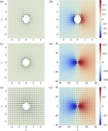
In figure 2 on the left we plot the leading-order velocity field,
 $\boldsymbol{u}_{s}^{(0)}$
overlaid on the concentration field
 ${\it\Gamma}_{0}=1$
and on the right we plot the Marangoni flow,
 $\boldsymbol{u}_{s}^{(1)}$
, overlaid on the perturbation in the concentration field
 ${\it\Gamma}_{1}$
. We show as illustrative examples: (a,b) an essentially inviscid interface,
 $\mathit{Bo}_{1}=0.01$
,
 ${\it\alpha}=1$
; (c,d) an interface with very weak shear viscosity but strong dilatational viscosity,
 $\mathit{Bo}_{1}=0.01$
,
 $\mathit{Bo}_{2}=5$
(
 ${\it\alpha}\approx 10^{4}$
); (e,f) an interface with high shear viscosity but no dilatational viscosity,
 $\mathit{Bo}_{1}=10$
,
 ${\it\alpha}=0$
. We see in each instance that the leading-order flow field causes a surplus of surfactant in front of the leading edge of the disk and a deficit behind the trailing edge. This perturbation decays as
 $1/r$
(see (3.60)) and induces a front to back Marangoni flow on the probe at
 $\mathit{O}(Pe_{s})$
that imparts an additional force on the disk. Increasing the dilatational viscosity diminishes the strength of the concentration perturbation (as shown in figure 2
c,d) and at large values the interface approaches an incompressible flow (equal exactly when
 ${\it\alpha}\rightarrow \infty$
). We also see that increasing the surface shear viscosity supresses surface vortices in the base flow and causes the interface to move more uniformly to minimize surface shear (as shown in figure 2
e,f).
Vector plot of the leading-order velocity field
 $\boldsymbol{u}_{s}^{(0)}$
(a,c,e) and Marangoni flow
 $\boldsymbol{u}_{s}^{(1)}$
(b,d,f) overlaid on the leading-order concentration field
 ${\it\Gamma}_{0}$
(a,c,e) and concentration field perturbation
 ${\it\Gamma}_{1}$
(b,d,f). (a,b) Nearly inviscid interface
 $\mathit{Bo}_{1}=0.01$
,
 ${\it\alpha}=1$
; (c,d) low shear and large dilatational viscosity
 $\mathit{Bo}_{1}=0.01$
,
 $\mathit{Bo}_{2}=5$
(
 ${\it\alpha}\approx 10^{4}$
); (e,f) large shear and no dilatational viscosity
 $\mathit{Bo}_{1}=10$
,
 ${\it\alpha}=0$
.

3.4.2 Force on the disk
The force on the probe at each order is given by the sum of the bulk and interfacial forces (2.19). Taking
 $\boldsymbol{F}$
to be represented by an expansion in
 $Pe_{s}$
we find that
 $$\begin{eqnarray}\displaystyle \boldsymbol{F}=-2{\rm\pi}\boldsymbol{e}_{x}[\hat{F}_{0}+Ma\hat{F}_{1}]+\mathit{O}(Pe_{s}^{2}), & & \displaystyle\end{eqnarray}$$
where
 $$\begin{eqnarray}\displaystyle Ma=\frac{Pe_{s}}{{\it\beta}}=\frac{{\it\delta}E_{0}a}{{\it\eta}D_{s}}, & & \displaystyle\end{eqnarray}$$
is a Marangoni number and
 $$\begin{eqnarray}\displaystyle & \displaystyle \hat{F}_{0}=\frac{4\text{K}_{2}(1/\mathit{Bo}_{2})\text{K}_{2}(1/\mathit{Bo}_{1})}{4\text{K}_{2}(1/\mathit{Bo}_{2})\text{K}_{0}(1/\mathit{Bo}_{1})+\text{K}_{0}(1/\mathit{Bo}_{2})\text{K}_{2}(1/\mathit{Bo}_{1})}, & \displaystyle\end{eqnarray}$$
 $$\begin{eqnarray}\displaystyle & \displaystyle \hat{F}_{1}=\frac{\left(\text{K}_{0}(1/\mathit{Bo}_{2})^{2}+\text{K}_{1}(1/\mathit{Bo}_{2})^{2}\right)\text{K}_{2}(1/\mathit{Bo}_{1})^{2}}{\left(4\text{K}_{2}(1/\mathit{Bo}_{2})\text{K}_{0}(1/\mathit{Bo}_{1})+\text{K}_{0}(1/\mathit{Bo}_{2})\text{K}_{2}(1/\mathit{Bo}_{1})\right)^{2}}. & \displaystyle\end{eqnarray}$$
 $\hat{F}_{0}$
represents the force on a probe translating through an interface at a rate slow enough that the surfactant concentration at the interface, and hence the surface pressure, can be assumed to be homogeneous and constant. Now when the probe moves with a finite velocity, corresponding to a small but finite value of the Péclet number, perturbations in the concentration field arise as a consequence of the convection of surfactant by the flow field. These variations in the concentration lead to a Marangoni flow, whose strength is modulated by the interfacial ‘stiffness’
 ${\it\beta}^{-1}$
, and ultimately an additional force felt by the probe due to this flow. The Marangoni number,
 $Ma=Pe_{s}{\it\beta}^{-1}$
, therefore sets the magnitude of the force due to the perturbations in the concentration field (Marangoni force). The Marangoni number must be small for the asymptotic validity of this expansion and in the simplest terms this implies a dilute interface. As mentioned previously, the compressibility of a surfactant laden interface may often be small, particularly if surfactant at the interface is near a maximum concentration.
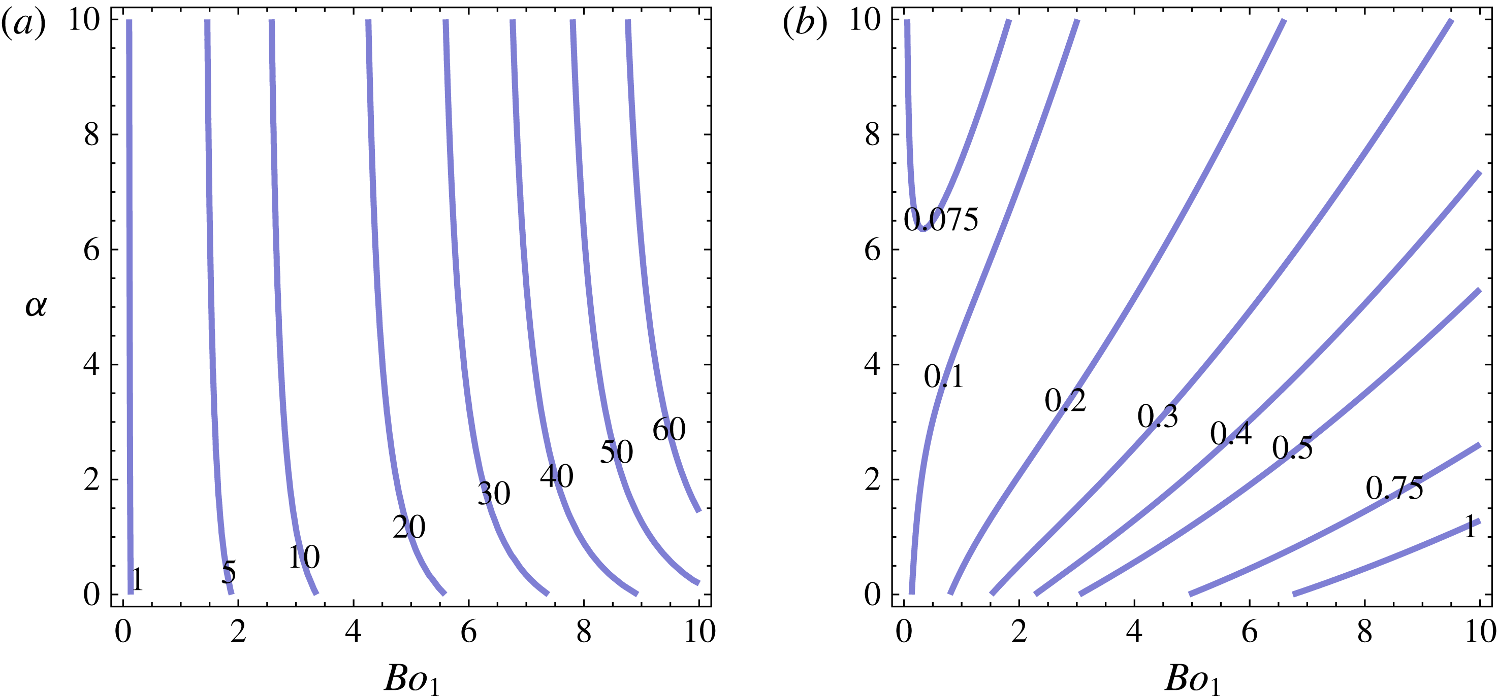
Contour plots of the non-dimensional coefficients for the force on a slow probe,
 $\hat{F}_{0}$
, in (a) and the force due to Marangoni flow,
 $\hat{F}_{1}$
, in (b), varying
 $\mathit{Bo}_{1}$
and viscosity ratio
 ${\it\alpha}$
when
 $Pe_{s}\ll 1$
.

Recalling that
 $\mathit{Bo}_{1}^{2}={\it\eta}_{s}H/{\it\eta}a^{2}$
while
 $\mathit{Bo}_{2}^{2}=({\it\kappa}_{s}+{\it\eta}_{s})H/4{\it\eta}a^{2}$
we see that both the equilibrated force,
 $\hat{F}_{0}$
, and the Marangoni force,
 $\hat{F}_{1}$
, depend non-trivially on the surface viscosities. We show contours of
 $\hat{F}_{0}$
and
 $\hat{F}_{1}$
against
 $\mathit{Bo}_{1}$
and the viscosity ratio
 ${\it\alpha}$
in figure 3 and note that both forces are strictly non-negative, meaning they both oppose the motion of the probe. Both components of the force are also finite in the limit of vanishing surface viscosities as one might expect on physical grounds as the probe still feels the bulk flow even if the interface is inviscid.
Ascertaining a surface viscosity from a force measurement would require knowledge of either
 $\mathit{Bo}_{1}$
or
 ${\it\alpha}$
as well as knowledge of the Marangoni number in which is embedded the relaxation time scale as well as the compressibility of the interface. Extracting a dilatational viscosity for instance, from a measured force magnitude,
 $F_{m}$
, given knowledge of all other parameters would involve resolution of the nonlinear algebraic equation
 $\hat{F}_{0}({\it\alpha})+Ma\hat{F}_{1}({\it\alpha})=F_{m}/2{\rm\pi}$
for
 ${\it\alpha}$
. As an example of peril, if
 $F_{m}\approx \text{K}_{2}(1/\mathit{Bo}_{1})/\text{K}_{0}(1/\mathit{Bo}_{1})$
then
 ${\it\alpha}$
may vary several orders in magnitude for very small changes in the measurement. In order to develop insight into the dependence of these forces on the surface viscosities we explore various limiting cases below.
First we observe that in the limit of small surface viscosities (as shown in figure 2
a), the interface, to leading order, is equivalent to a clean interface with no surfactant present (Barentin et al.
Reference Barentin, Ybert, Di Meglio and Joanny1999). Calculating the force, assuming
 $\mathit{Bo}_{1}\ll 1$
with
 ${\it\alpha}=\mathit{O}(1)$
, we obtain
 $$\begin{eqnarray}\displaystyle & \displaystyle \hat{F}_{0}={\textstyle \frac{4}{5}}+{\textstyle \frac{4}{25}}(8+\sqrt{1+{\it\alpha}})\mathit{Bo}_{1}+\mathit{O}(\mathit{Bo}_{1}^{2}), & \displaystyle\end{eqnarray}$$
 $$\begin{eqnarray}\displaystyle & \displaystyle \hat{F}_{1}={\textstyle \frac{2}{25}}+{\textstyle \frac{1}{250}}(64-27\sqrt{1+{\it\alpha}})\mathit{Bo}_{1}+\mathit{O}(\mathit{Bo}_{1}^{2}). & \displaystyle\end{eqnarray}$$
 $\hat{F}_{0}=4/5$
, in contrast, for an incompressible inviscid interface we found
 $\hat{F}_{0}=1$
. The Marangoni force is also finite when surface viscosities vanish, due to the Marangoni flow induced bulk drag on the bottom surface of the disk. From (3.66) and (3.67) we see that while the introduction of a surface dilatational viscosity increases the equilibrated drag on the disk, it decreases the Marangoni force felt by the probe by suppressing concentration perturbations (as illustrated in figure 2
b). In the large surface dilatational viscosity limit,
 ${\it\alpha}\rightarrow \infty$
we recover an incompressible interface and obtain
 $$\begin{eqnarray}\displaystyle & \displaystyle \hat{F}_{0}=\frac{\text{K}_{2}(1/\mathit{Bo}_{1})}{\text{K}_{0}(1/\mathit{Bo}_{1})},\quad {\it\alpha}\rightarrow \infty , & \displaystyle\end{eqnarray}$$
 $$\begin{eqnarray}\displaystyle & \displaystyle \hat{F}_{1}=0,\quad {\it\alpha}\rightarrow \infty . & \displaystyle\end{eqnarray}$$
 $Ma=0$
) varies smoothly from
 $\hat{F}_{0}=4/5$
to
 $\hat{F}_{0}=1$
as a function of surface dilatational viscosity (with zero surface shear viscosity). In contrast, the Marangoni force decays monotonically with increasing dilatational viscosity from
 $\hat{F}_{1}=2/25$
to zero with
 $\hat{F}_{1}\sim 1/(8\mathit{Bo}_{2})^{2}$
for large dilatational viscosities. This shows quantitatively that an interface with a large dilatational viscosity may behave as incompressible, despite a small Marangoni number, because of the large energy penalty (dissipation) associated with compressional flow.
In contrast to dilatational viscosity, both
 $\hat{F}_{0}$
and
 $\hat{F}_{1}$
increase monotonically with surface shear viscosity. The former is clear as one would expect more drag on the probe from a more viscous interface, but an increase in surface shear viscosity also increases the Marangoni flow induced drag on the disk. We eliminate surface dilatational viscosity, by setting
 ${\it\alpha}=0$
, then in the limit of large surface shear viscosities (as shown in figure 2
c) we obtain
 $$\begin{eqnarray}\displaystyle & \displaystyle \hat{F}_{0}\sim \frac{2\mathit{Bo}_{1}^{2}}{\ln \left(2\mathit{Bo}_{1}^{2}\right)-2{\it\gamma}}, & \displaystyle\end{eqnarray}$$
 $$\begin{eqnarray}\displaystyle & \displaystyle \hat{F}_{1}\sim \frac{\mathit{Bo}_{1}^{2}}{4\left(\ln \left(2\mathit{Bo}_{1}^{2}\right)-2{\it\gamma}\right)^{2}}, & \displaystyle\end{eqnarray}$$
 ${\it\gamma}$
is the Euler–Mascheroni constant. Both coefficients diverge for large surface shear viscosities, while the ratio
 $\hat{F}_{1}/\hat{F}_{0}\rightarrow 0$
logarithmically slowly, so only for very large Boussinesq numbers can one reasonably neglect the Marangoni component. We also note that the difference in the force between the compressible and incompressible interface (given by (3.31)) grows more pronounced as the surface shear viscosity increases.
Note that above we found that one may obtain the same force on the probe if the interface is nearly incompressible or has a very large dilatational viscosity. This points to a central issue in interfacial rheology, the force felt by a probe depends non-trivially not only on the interfacial viscosities but also the time scales of the mechanisms that minimize concentration gradients (and thus Marangoni forces) on the interface. If these are not known (or are erroneous), estimates of material parameters from a force measured on the probe may be significantly flawed.
Finally we note that the Marangoni force on the probe may also be found without resolution of the Marangoni flow itself, at the expense of integrals over the viscous interface, by way of the Lorentz reciprocal theorem. Such an approach also serves as a useful check of the flow field calculations. A derivation is included for reference in appendix B.
3.5 Fast adsorption
$({\it\epsilon}\ll 1;~Pe_{s}=\mathit{O}(1))$

We now explore the limit in which the absorption/desorption time scale is much faster than the convective time scale (
 ${\it\epsilon}\ll 1$
). We assume that
 $Pe_{s}=\mathit{O}(1)$
, which implies that the adsorption/desorption process relaxes concentration gradients much more quickly than diffusion. In the fast adsorption/desorption limit,
 ${\it\epsilon}\rightarrow 0$
, the reaction process is instantaneous and the concentration of surfactant remains at its equilibrium value,
 ${\it\Gamma}=1$
. To examine small deviations from this limit we again posit a regular perturbation expansion, now in
 ${\it\epsilon}$
, for all fields, e.g.
 ${\it\Gamma}(\boldsymbol{x})=\sum _{n}{\it\epsilon}^{n}{\it\Gamma}_{n}$
, etc. Upon substitution of these expansions into the surfactant conservation equation (3.12) we find at
 $\mathit{O}(1)$
and
 $\mathit{O}({\it\epsilon})$
,
 $$\begin{eqnarray}\displaystyle & \displaystyle {\it\Gamma}_{0}=1, & \displaystyle\end{eqnarray}$$
 $$\begin{eqnarray}\displaystyle & \displaystyle {\it\Gamma}_{1}=-\boldsymbol{{\rm\nabla}}_{s}\boldsymbol{\cdot }\boldsymbol{u}_{s}^{(0)}. & \displaystyle\end{eqnarray}$$
 $$\begin{eqnarray}\displaystyle \boldsymbol{{\rm\nabla}}_{s}{\it\Pi}={\it\epsilon}{\it\beta}^{-1}\boldsymbol{{\rm\nabla}}_{s}{\it\Gamma}_{1}+\mathit{O}({\it\epsilon}^{2}), & & \displaystyle\end{eqnarray}$$
which will ultimately drive a Marangoni flow in response.
The equations of motion at leading order are identical to those given in § 3.4, as are the boundary conditions and although it may seem that the analysis should follow the low Péclet number case, a problem that arises here is that the
 $\mathit{O}({\it\epsilon})$
approximation of the surfactant conservation equation does not contain the Laplacian term and is therefore of lower order than the original equation. As a consequence, it is not possible, in general, to satisfy all the boundary conditions on
 ${\it\Gamma}_{1}$
. In particular, though the leading-order approximation
 ${\it\Gamma}_{0}$
trivially satisfies all boundary conditions, the first-order solution
 ${\it\Gamma}_{1}$
cannot satisfy the no-flux condition at
 $r=1$
, and hence the expansion in
 ${\it\epsilon}$
is singular. To see this we need only note that the solution for the zeroth-order velocity field satisfies
 $$\begin{eqnarray}\displaystyle \boldsymbol{{\rm\nabla}}_{s}\boldsymbol{\cdot }\boldsymbol{u}_{s}^{(0)}=c_{1}\text{K}_{1}(r/\mathit{Bo}_{1})\cos {\it\theta}, & & \displaystyle\end{eqnarray}$$
and by substitution into (3.73) one can verify that
 ${\it\Gamma}_{1}$
cannot satisfy the no-flux boundary condition.
Clearly, there must exist a length scale over which diffusion matters, namely, a boundary layer. To solve for the concentration profile over the whole domain we appeal to the method of matched asymptotic expansions (Hinch Reference Hinch1991). The expansion above is then seen as an outer solution for which the far-field boundary conditions are satisfied, but which we must match to an inner boundary layer solution that satisfies the boundary conditions at the disk perimeter. However, we will show that ultimately the boundary layer does not affect the first two terms of the force on the probe and so relegate a brief description of the boundary layer analysis to appendix C.
3.5.1 Solution of flow field
The outer solution follows the approach described previously in the small
 $Pe_{s}$
expansion in § 3.2, indeed the zeroth-order solution is identical. The first difference from the small
 $Pe_{s}$
expansion arises from the surface pressure term in (3.38) for
 $n=1$
. Taking the divergence of (3.74) and utilizing (3.73) we obtain
 $$\begin{eqnarray}\displaystyle \boldsymbol{{\rm\nabla}}_{s}^{2}{\it\Pi}_{1}=-\frac{1}{{\it\beta}}{\rm\nabla}_{s}^{2}\boldsymbol{{\rm\nabla}}_{s}\boldsymbol{\cdot }\boldsymbol{u}_{s}^{(0)}=-\frac{1}{\mathit{Bo}_{2}^{2}{\it\beta}}\boldsymbol{{\rm\nabla}}_{s}\boldsymbol{\cdot }\boldsymbol{u}_{s}^{(0)}, & & \displaystyle\end{eqnarray}$$
where the second equality is obtained from (3.44). Finally then (3.41) for
 $n=1$
becomes
 $$\begin{eqnarray}\displaystyle \left(\mathit{Bo}_{2}^{2}{\rm\nabla}_{s}^{2}-1\right)\boldsymbol{{\rm\nabla}}_{s}\boldsymbol{\cdot }\boldsymbol{u}_{s}^{(1)}=-\frac{1}{4\mathit{Bo}_{2}^{2}{\it\beta}}\boldsymbol{{\rm\nabla}}_{s}\boldsymbol{\cdot }\boldsymbol{u}_{s}^{(0)}, & & \displaystyle\end{eqnarray}$$
which differs from the small
 $Pe_{s}$
case by only the factor
 $-\mathit{Bo}_{2}^{-2}$
in the right-hand side. Because of this the vorticity and divergence fields have the same functional form as in the small
 $Pe_{s}$
expansion, (3.58) and (3.59), but now with the coefficient
 $C_{1}=c_{1}/8{\it\beta}\mathit{Bo}_{2}^{2}$
.
We saw above that the concentration perturbation field is given directly by the divergence of the leading-order velocity field. The no-flux condition is satisfied at the disk boundary by means of a boundary layer and then combining the inner and outer solutions (see appendix C for details on resolving the boundary layer) we may write a uniformly valid expansion of the concentration field over the whole domain as
 $$\begin{eqnarray}\displaystyle {\it\Gamma}\sim 1-{\it\epsilon}\left[\boldsymbol{{\rm\nabla}}_{s}\boldsymbol{\cdot }\boldsymbol{u}_{s}^{(0)}+\sqrt{\frac{{\it\epsilon}}{Pe_{s}}}\text{e}^{-\sqrt{Pe_{s}/{\it\epsilon}}(r-1)}\left.\partial _{r}(\boldsymbol{{\rm\nabla}}_{s}\boldsymbol{\cdot }\boldsymbol{u}_{s}^{(0)})\right|_{r=1}\right]. & & \displaystyle\end{eqnarray}$$
It is important to note that the outer solution of the concentration field is correct up to
 $\mathit{O}({\it\epsilon})$
and hence the force on the disk due to the surface pressure
 ${\it\Pi}$
from the outer solution will also be accurate up to this order while the correction due to the boundary layer occurs at
 $\mathit{O}({\it\epsilon}^{3/2})$
. We also find that the outer solution for the flow field is valid over the entire domain up to
 $\mathit{O}({\it\epsilon})$
. A uniformly valid solution may be written as
 $$\begin{eqnarray}\displaystyle \boldsymbol{u}_{s}=\boldsymbol{u}_{s}^{(0)}+{\it\epsilon}\boldsymbol{u}_{s}^{(1)}+{\it\epsilon}^{2}\left[\boldsymbol{u}_{s}^{(2)}+\boldsymbol{e}_{r}\frac{1}{4{\it\beta}\mathit{Bo}_{2}^{2}Pe_{s}}\text{e}^{-\sqrt{Pe_{s}/{\it\epsilon}}(r-1)}\left.\partial _{r}(\boldsymbol{{\rm\nabla}}_{s}\boldsymbol{\cdot }\boldsymbol{u}_{s}^{(0)})\right|_{r=1}\right]. & & \displaystyle\end{eqnarray}$$
The correction due to the boundary layer occurs at
 $\mathit{O}({\it\epsilon}^{2})$
. We are interested in the force on the probe and we see that radial gradients at the disk perimeter
 $\partial D$
would have corrections of
 $\mathit{O}({\it\epsilon}^{3/2})$
, and similarly the surface pressure field evaluated on
 $\partial D$
leads to a correction of
 $\mathit{O}({\it\epsilon}^{3/2})$
. We conclude that the outer solution provides the correct force on the probe up to
 $\mathit{O}({\it\epsilon})$
.
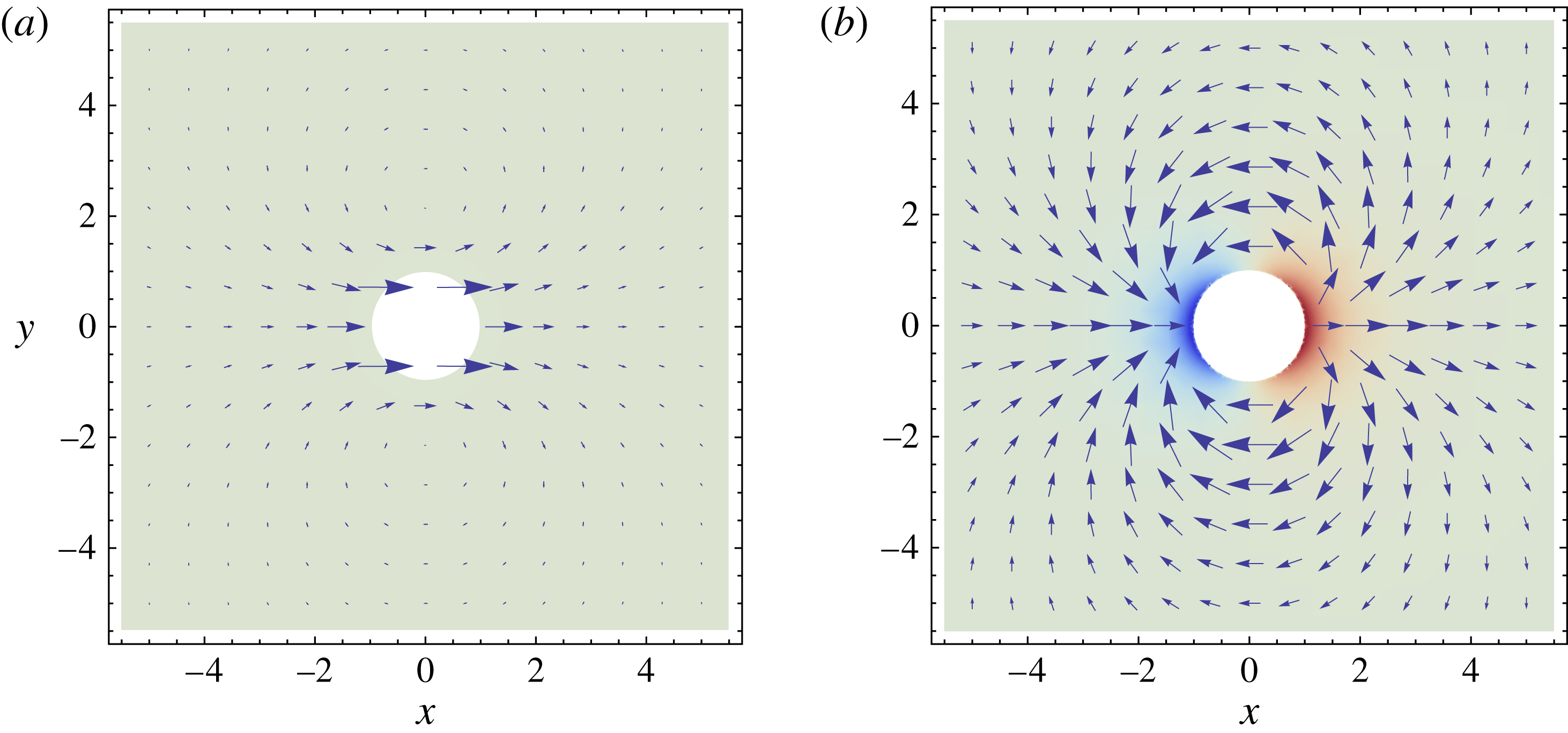
As an illustrative example of Marangoni flows due to finite absorption/desorption time scales in figure 4(a), the leading-order velocity field
 $\boldsymbol{u}_{s}^{(0)}$
is shown for
 $\mathit{Bo}_{1}=1$
with viscosity ratio
 ${\it\alpha}=1$
(
 $\mathit{Bo}_{2}=1/\sqrt{2}$
) overlaid on the concentration field
 ${\it\Gamma}_{0}=1$
. In figure 4(b) we plot the Marangoni flow
 $\boldsymbol{u}_{s}^{(1)}$
overlaid on the perturbation in the concentration field
 ${\it\Gamma}_{1}$
. Again we see that the leading-order flow field causes a surplus of surfactant at the front edge of the disk and a deficit at the rear edge as in the case of a small Péclet expansion; however, here the surfactant perturbation decays exponentially quickly with radial distance away from the probe. The Marangoni flow is also qualitatively similar, driving flow from front to back thus increasing the force felt by the probe.
Vector plot of the leading-order velocity field
 $\boldsymbol{u}_{s}^{(0)}$
(a) and Marangoni flow
 $\boldsymbol{u}_{s}^{(1)}$
(b) overlaid on the leading-order concentration field
 ${\it\Gamma}_{0}$
(a) and concentration field perturbation
 ${\it\Gamma}_{1}$
(b). Here
 $\mathit{Bo}_{1}=1$
and
 ${\it\alpha}=1$
.

3.5.2 Force on the disk
With the solution of the flow field we can compute the force on the translating probe
 $$\begin{eqnarray}\displaystyle \boldsymbol{F}=-2{\rm\pi}\boldsymbol{e}_{x}[\hat{F}_{0}+Ma\hat{F}_{1}]+\mathit{O}({\it\epsilon}^{2}), & & \displaystyle\end{eqnarray}$$
where here
 $$\begin{eqnarray}\displaystyle Ma=\frac{{\it\epsilon}}{{\it\beta}}=\frac{{\it\delta}E_{0}}{k_{s}{\it\eta}a} & & \displaystyle\end{eqnarray}$$
is another Marangoni number. The force on a probe moving slowly enough that the interface is at equilibrium,
 $\hat{F}_{0}$
, is identical to the formula given previously in (3.64). Slow but finite disk speeds lead to variations in the concentration field of
 $\mathit{O}({\it\epsilon})$
which drive a Marangoni flow modulated by the interfacial compressibility
 ${\it\beta}$
and yield an additional force given by
 $$\begin{eqnarray}\displaystyle \hat{F}_{1}=\frac{\left(\text{K}_{0}(1/\mathit{Bo}_{2})\text{K}_{2}(1/\mathit{Bo}_{2})-\text{K}_{1}(1/\mathit{Bo}_{2})^{2}\right)\text{K}_{2}(1/\mathit{Bo}_{1})^{2}}{\mathit{Bo}_{2}^{2}\left(4\text{K}_{0}(1/\mathit{Bo}_{1})\text{K}_{2}(1/\mathit{Bo}_{2})+\text{K}_{0}(1/\mathit{Bo}_{2})\text{K}_{2}(1/\mathit{Bo}_{1})\right)^{2}}. & & \displaystyle\end{eqnarray}$$
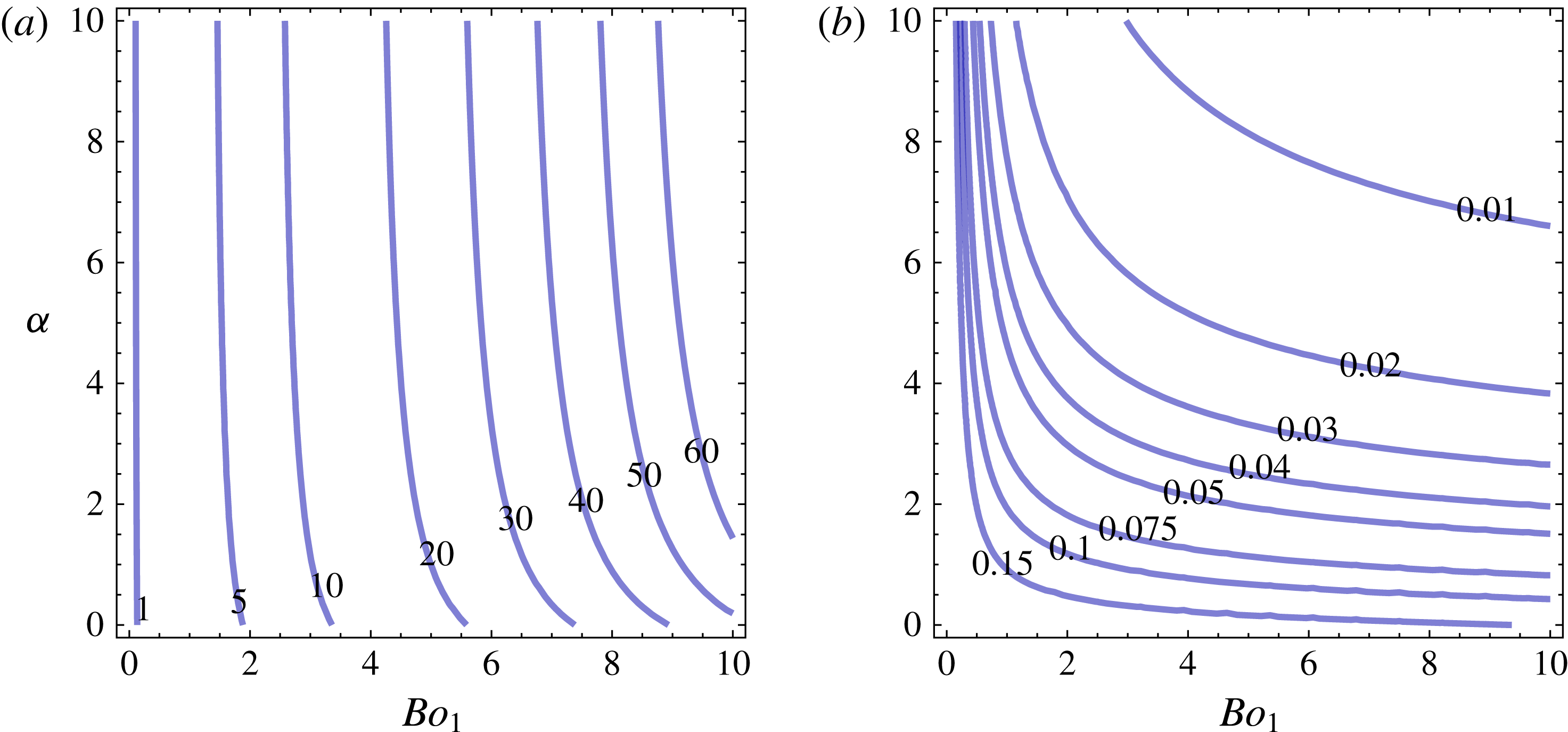
In figure 5 we show contours of
 $\hat{F}_{1}$
(alongside
 $\hat{F}_{0}$
for comparison) against
 $\mathit{Bo}_{1}$
and the viscosity ratio
 ${\it\alpha}$
.
At the small surface viscosities
 $\mathit{Bo}_{1}\ll 1$
(and
 ${\it\alpha}=\mathit{O}(1)$
) we obtain
 $$\begin{eqnarray}\displaystyle \hat{F}_{1}\sim \frac{2}{25\mathit{Bo}_{1}\sqrt{1+{\it\alpha}}}=\frac{1}{25\mathit{Bo}_{2}}. & & \displaystyle\end{eqnarray}$$
In contrast to the diffusive case, we discover here that the Marangoni force diverges with vanishing surface viscosities (scaling as
 $1/\sqrt{{\it\eta}_{s}+{\it\kappa}_{s}}$
). This is clearly an unphysical result. By looking simply at a balance of bulk drag and surface pressure we expect
 $\hat{F}_{1}\rightarrow \text{const.}$
as observed in the small Péclet expansion. Ultimately we believe this arises from the fact that the lubrication limit is singular for vanishing surface viscosities. Looking more carefully, we see that as
 $\mathit{Bo}_{1}\rightarrow 0$
we have a velocity discontinuity at the boundary and hence an expansion rate that diverges as
 $\boldsymbol{{\rm\nabla}}_{s}\boldsymbol{\cdot }\boldsymbol{u}_{s}^{(0)}(r=1)\sim -(2/5)\mathit{Bo}_{2}^{-1}$
which is particularly problematic as this term directly yields the first-order concentration field and ultimately drives the Marangoni flow. However, the velocity discontinuity at the boundary in the lubrication limit is otherwise smoothed by the presence of a finite surface viscosities.
Contour plots of the non-dimensional coefficients for the force on a slow probe,
 $\hat{F}_{0}$
, in (a), and the force due to Marangoni flow,
 $\hat{F}_{1}$
, in (b), varying
 $\mathit{Bo}_{1}$
and viscosity ratio
 ${\it\alpha}$
when
 ${\it\epsilon}\ll 1$
.

Unlike in the small Péclet case, where surface shear viscosity increases the magnitude of the Marangoni force, for surface perturbations arising due to a finite/adsorption desorption time scale, the Marangoni force strictly decays with increasing surface viscosities, both shear and dilatational. For large surface shear viscosities, the Marangoni force decays logarithmically slowly, for
 $\mathit{Bo}_{1}\gg 1$
(
 ${\it\alpha}=0$
) we find
 $$\begin{eqnarray}\displaystyle \hat{F}_{1}\sim \frac{\ln \left[\mathit{Bo}_{1}^{2}/e\right]-2{\it\gamma}}{\left(\ln \left[2\mathit{Bo}_{1}^{2}\right]-2{\it\gamma}\right)^{2}}. & & \displaystyle\end{eqnarray}$$
Herein lies a relevant physical distinction and an important physical insight from the present analysis: the surface viscosities affect the Marangoni force differently depending on the time scales of the relaxation mechanisms for surfactant concentration variations. When the diffusive time scale is much faster than the adsorption/desorption time scale, the surface shear viscosity acts to increase the Marangoni force, whereas when the adsorption/desorption is faster, the surface shear viscosity diminishes the Marangoni force. The difference is that the concentration perturbations in the former case tend to a finite value for large surface shear viscosities whereas in latter case the concentration perturbations decay to zero.
Large dilatational viscosities diminish the Marangoni force as well in this case and we again find that in the limit
 $$\begin{eqnarray}\displaystyle \hat{F}_{1}=0,\quad {\it\alpha}\rightarrow \infty , & & \displaystyle\end{eqnarray}$$
in other words, for very large surface dilatational viscosities the Marangoni force vanishes and the force felt by the probe is the same as that measured at an incompressible interface.
4 Concluding remarks
In this paper we have calculated the force on a probe at an interface laden with soluble surfactant. We derived analytically the Marangoni force on a disk-shaped probe translating through the interface of a thin film at a finite time scale and in particular we demonstrated the physical effect that interfacial viscosities have on Marangoni forces felt by the probe. A translating probe in an initially equilibrated interface imparts a dilatational flow field on the interface that in turn leads to surfactant concentration variations. These flows depend intrinsically on the mechanical properties of the interface, namely the dilatational and shear viscosities and hence so do the concentration variations. Surfactant inhomogeneity leads to Marangoni flows due to variations in surface tension but these flows also depend directly on the surface viscosities of the interface. Importantly, we show that surface viscosities can have a completely different effect on the Marangoni force felt by the probe depending on the governing time scale of the problem, in particular on whether or not the adsorption/desorption time scale is fast or slow relative to the diffusive time scale. We also show that the effect on the probe due to non-zero values of the dilatational viscosity can be indistinguishable from those due to surface elasticity. These factors make it extremely difficult to determine quantitatively the origin of the force on the probe, and make it extremely difficult, if not impossible, to infer values of the surface viscosities from experimental measurements of the force. Clearly, a translating probe with the shape of a disk is not at all optimal as a probe for interfacial viscosities, and one may infer that the same would be true for any probe that produces a mixed-type flow at the interface and therefore that methods that produce either pure shear (Zell et al. Reference Zell, Nowbahar, Mansard, Leal, Deshmukh, Mecca, Tucker and Squires2014) or dilatation (Kotula & Anna Reference Kotula and Anna2015) should be preferred. Admittedly, we have only considered specialized cases where the surfactant concentration is nearly uniform, and numerical methods would be needed to solve for more general cases. However, we expect the qualitative message from the present work to be reflected for more general cases: namely, that the contributions to the force on a translating probe due to Marangoni effects (i.e. interface elasticity) and non-zero surface viscosities will be tangled in ways that make such a translating probe (which produces a mixed-type flow) ineffective for determining the rheological characteristics of the interface.
Acknowledgement
Funding by the NSF (CBET-0932259) is gratefully acknowledged.
Appendix A. Bulk concentration
Although we have assumed the adsorption rate is constant, it will in fact depend on the bulk concentration
 $c$
, at the wall
 $k_{s}(c_{s})$
where
 $$\begin{eqnarray}\displaystyle c_{s}\equiv \lim _{z\rightarrow 1}c(y). & & \displaystyle\end{eqnarray}$$
Species conservation yields the flux boundary condition
 $$\begin{eqnarray}\displaystyle \frac{\partial c}{\partial n}=Da({\it\epsilon}{\it\Gamma}_{1}+\cdots \,), & & \displaystyle\end{eqnarray}$$
where the Damköhler number
 $Da=({\it\Gamma}_{0}/c_{0}H)(k_{s}H^{2}/D)$
(Probstein Reference Probstein1994) and
 $D$
is the bulk diffusivity and
 $c_{0}$
is the bulk concentration at equilibrium. In order for our assumption of a constant reaction rate
 $k_{s}$
to be valid asymptotically to the order of the calculation we require
 $$\begin{eqnarray}\displaystyle {\it\epsilon}Da=\frac{{\it\Gamma}_{0}}{c_{0}H}\frac{H^{2}/D}{a/U}\ll \mathit{O}({\it\epsilon}), & & \displaystyle\end{eqnarray}$$
in other words we want
 $Da\ll \mathit{O}(1)$
so that the bulk flux is zero to
 $\mathit{O}({\it\epsilon})$
and hence the bulk may be considered constant
 $c=c_{s}$
to linear order.
Appendix B. Reciprocal theorem for the Marangoni force
At a viscous compressible interface conservation of momentum gives
 $\boldsymbol{{\rm\nabla}}_{s}\boldsymbol{\cdot }{\bf\sigma}_{s}=-\boldsymbol{f}_{s}$
while in the incompressible bulk subphase we have
 $\boldsymbol{{\rm\nabla}}\boldsymbol{\cdot }{\bf\sigma}=\mathbf{0}$
. The traction exerted by the subphase is given by
 $\boldsymbol{f}_{s}=-\boldsymbol{n}\boldsymbol{\cdot }{\bf\sigma}$
defining the normal to point out of the subphase fluid.
We shall take as an auxiliary problem (denoted by a hat) the solution of the probe moving through a viscous equilibrated interface,
 $\hat{{\it\Pi}}_{s}=\text{constant}$
(i.e. when
 $Pe\rightarrow 0$
or
 ${\it\epsilon}\rightarrow 0$
). We may write the following expression
 $$\begin{eqnarray}\displaystyle \int _{V}\hat{\boldsymbol{u}}\boldsymbol{\cdot }(\boldsymbol{{\rm\nabla}}\boldsymbol{\cdot }{\bf\sigma})\,\text{d}V=\int _{V}\boldsymbol{u}\boldsymbol{\cdot }(\boldsymbol{{\rm\nabla}}\boldsymbol{\cdot }\hat{{\bf\sigma}})\,\text{d}V, & & \displaystyle\end{eqnarray}$$
for the entire fluid,
 $V$
, as both sides are trivially zero. Applying the divergence theorem while enforcing the incompressibility of the bulk phase we obtain
 $$\begin{eqnarray}\displaystyle \int _{S}\boldsymbol{n}\boldsymbol{\cdot }({\bf\sigma}\boldsymbol{\cdot }\hat{\boldsymbol{u}}-\hat{{\bf\sigma}}\boldsymbol{\cdot }\boldsymbol{u})\,\text{d}S=0. & & \displaystyle\end{eqnarray}$$
We divide the surface
 $S$
bounding
 $V$
into the viscous interface
 $S_{s}$
the disk base
 $D$
the solid boundary and the fluid at infinity. The term at infinity decays faster than
 $r^{-2}$
while the velocity on the boundary is zero by the no-slip condition. Taking
 $\boldsymbol{n}\boldsymbol{\cdot }{\bf\sigma}=\boldsymbol{{\rm\nabla}}_{s}\boldsymbol{\cdot }{\bf\sigma}_{s}$
at the interface and noting that the no-slip condition gives
 $\boldsymbol{u}=\boldsymbol{U}$
and
 $\hat{\boldsymbol{u}}=\hat{\boldsymbol{U}}$
on the disk we have then
 $$\begin{eqnarray}\displaystyle \boldsymbol{U}\boldsymbol{\cdot }\hat{\boldsymbol{F}}_{D}-\hat{\boldsymbol{U}}\boldsymbol{\cdot }\boldsymbol{F}_{D}+\int _{S_{s}}(\boldsymbol{{\rm\nabla}}_{s}\boldsymbol{\cdot }{\bf\sigma}_{s}\boldsymbol{\cdot }\hat{\boldsymbol{u}}-\boldsymbol{{\rm\nabla}}_{s}\boldsymbol{\cdot }\hat{{\bf\sigma}}_{s}\boldsymbol{\cdot }\boldsymbol{u})\,\text{d}S=0, & & \displaystyle\end{eqnarray}$$
where
 $\boldsymbol{F}_{D}$
is the force on the disk due to the subphase. Another application of the divergence theorem while discarding the terms which decay at infinity leads to
 $$\begin{eqnarray}\displaystyle \boldsymbol{U}\boldsymbol{\cdot }\hat{\boldsymbol{F}}_{D}-\hat{\boldsymbol{U}}\boldsymbol{\cdot }\boldsymbol{F}_{D}-\int _{\partial D}\boldsymbol{n}_{s}\boldsymbol{\cdot }({\bf\sigma}_{s}\boldsymbol{\cdot }\hat{\boldsymbol{u}}-\hat{{\bf\sigma}}_{s}\boldsymbol{\cdot }\boldsymbol{u})\,\text{d}l=\int _{S_{s}}({\bf\sigma}_{s}\boldsymbol{ : }\boldsymbol{{\rm\nabla}}_{s}\hat{\boldsymbol{u}}-\hat{{\bf\sigma}}_{s}\boldsymbol{ : }\boldsymbol{{\rm\nabla}}_{s}\boldsymbol{u})\,\text{d}S. & & \displaystyle\end{eqnarray}$$
Here we define
 $\boldsymbol{n}_{s}$
as the normal to the disk facing into the interface. Applying the no-slip condition we obtain
 $$\begin{eqnarray}\displaystyle \hat{\boldsymbol{U}}\boldsymbol{\cdot }(\boldsymbol{F}_{D}+\boldsymbol{F}_{s})-\boldsymbol{U}\boldsymbol{\cdot }(\hat{\boldsymbol{F}}_{D}+\hat{\boldsymbol{F}}_{s})=\int _{S_{s}}(\hat{{\bf\sigma}}_{s}\boldsymbol{ : }\boldsymbol{{\rm\nabla}}_{s}\boldsymbol{u}-{\bf\sigma}_{s}\boldsymbol{ : }\boldsymbol{{\rm\nabla}}_{s}\hat{\boldsymbol{u}})\,\text{d}S, & & \displaystyle\end{eqnarray}$$
where
 $\boldsymbol{F}_{s}$
represents the force on the disk due to the interface. Now recalling the form of the stress tensor at the interface, taking
 $\hat{{\it\eta}}_{s}={\it\eta}_{s}$
and
 $\hat{{\it\kappa}}_{s}={\it\kappa}_{s}$
, we may recast the above as
 $$\begin{eqnarray}\displaystyle \hat{\boldsymbol{U}}\boldsymbol{\cdot }\boldsymbol{F}-\boldsymbol{U}\boldsymbol{\cdot }\hat{\boldsymbol{F}}=\int _{S_{s}}({\it\Pi}_{s}\boldsymbol{{\rm\nabla}}_{s}\boldsymbol{\cdot }\hat{\boldsymbol{u}}_{s}-\hat{{\it\Pi}}_{s}\boldsymbol{{\rm\nabla}}_{s}\boldsymbol{\cdot }\boldsymbol{u}_{s})\,\text{d}S, & & \displaystyle\end{eqnarray}$$
where the total force on the disk
 $\boldsymbol{F}=\boldsymbol{F}_{D}+\boldsymbol{F}_{s}$
. Yet another application of the divergence theorem, noting
 $\hat{{\it\Pi}}_{s}=\text{constant}$
, leads to
 $$\begin{eqnarray}\displaystyle \hat{\boldsymbol{U}}\boldsymbol{\cdot }\boldsymbol{F}-\boldsymbol{U}\boldsymbol{\cdot }\hat{\boldsymbol{F}}=-\hat{\boldsymbol{U}}\boldsymbol{\cdot }\int _{\partial D}\boldsymbol{n}_{s}{\it\Pi}_{s}\,\text{d}l-\int _{S_{s}}\hat{\boldsymbol{u}}_{s}\boldsymbol{\cdot }\boldsymbol{{\rm\nabla}}_{s}{\it\Pi}_{s}\,\text{d}S. & & \displaystyle\end{eqnarray}$$
The interfacial flow field and thus the force on the disk in the auxiliary problem are linear in the translational velocity,
 $\hat{\boldsymbol{u}}_{s}=\hat{\unicode[STIX]{x1D642}}\boldsymbol{\cdot }\hat{\boldsymbol{U}}$
and
 $\hat{\boldsymbol{F}}=-\hat{\unicode[STIX]{x1D64D}}\boldsymbol{\cdot }\hat{\boldsymbol{U}}$
respectively hence, discarding the arbitrary
 $\hat{\boldsymbol{U}}$
, we obtain
 $$\begin{eqnarray}\displaystyle {\rm\Delta}\boldsymbol{F}=-\int _{\partial D}\boldsymbol{n}_{s}{\it\Pi}_{s}\,\text{d}l-\int _{S_{s}}\hat{\unicode[STIX]{x1D642}}\boldsymbol{\cdot }\boldsymbol{{\rm\nabla}}_{s}{\it\Pi}_{s}\,\text{d}S. & & \displaystyle\end{eqnarray}$$
Here
 ${\rm\Delta}\boldsymbol{F}=\boldsymbol{F}+\hat{\unicode[STIX]{x1D64D}}\boldsymbol{\cdot }\boldsymbol{U}$
represents the change in the force due to variations of the surfactant field. The first contribution to the change in force is due to variations of the surface pressure while the second term represents the change in the force due to surface traction caused by the Marangoni flow. This approach avoids solution of the flow field
 $\boldsymbol{u}_{s}$
at the expense of the surface integral over the interface. This derivation is similar to that shown for an inviscid interface (Masoud & Stone Reference Masoud and Stone2014) and incompressible interface (Stone & Masoud Reference Stone and Masoud2015).
Appendix C. Boundary layer analysis
To obtain the inner solution we rescale the radial coordinate at the disk perimeter such that diffusion and adsorption/desorption are asymptotically balanced. It is a simple matter to show
 $$\begin{eqnarray}\displaystyle r-1={\it\varepsilon}R, & & \displaystyle\end{eqnarray}$$
where
 ${\it\varepsilon}={\it\epsilon}^{1/2}$
. With this choice the gradient operator becomes
 $$\begin{eqnarray}\displaystyle \boldsymbol{{\rm\nabla}}=\frac{1}{{\it\varepsilon}}\left[\boldsymbol{e}_{r}\partial _{R}+\boldsymbol{e}_{{\it\theta}}\frac{{\it\varepsilon}}{{\it\varepsilon}R+1}\partial _{{\it\theta}}\right]\equiv {\it\varepsilon}^{-1}\tilde{\boldsymbol{{\rm\nabla}}}, & & \displaystyle\end{eqnarray}$$
and the rescaled surfactant transport equation is given by
 $$\begin{eqnarray}\displaystyle {\it\varepsilon}\tilde{\boldsymbol{{\rm\nabla}}}_{s}\boldsymbol{\cdot }(\tilde{{\it\Gamma}}\tilde{\boldsymbol{u}}_{s}^{\prime })=Pe_{s}^{-1}\tilde{{\rm\nabla}}_{s}^{2}\tilde{{\it\Gamma}}+(1-\tilde{{\it\Gamma}}), & & \displaystyle\end{eqnarray}$$
where tildes indicate functions of the inner variable. The rescaled momentum equation is
 $$\begin{eqnarray}\displaystyle & \displaystyle {\it\varepsilon}\tilde{\boldsymbol{{\rm\nabla}}}_{s}\tilde{{\it\Pi}}=\mathit{Bo}_{1}^{2}[\tilde{{\rm\nabla}}_{s}^{2}\tilde{\boldsymbol{u}}_{s}+{\it\alpha}\tilde{\boldsymbol{{\rm\nabla}}}_{s}(\tilde{\boldsymbol{{\rm\nabla}}}_{s}\boldsymbol{\cdot }\tilde{\boldsymbol{u}}_{s})]-{\it\varepsilon}{\textstyle \frac{1}{2}}\tilde{\boldsymbol{{\rm\nabla}}}_{s}\tilde{p}-{\it\varepsilon}^{2}\tilde{\boldsymbol{u}}_{s}, & \displaystyle\end{eqnarray}$$
 $$\begin{eqnarray}\displaystyle & \displaystyle \tilde{{\rm\nabla}}^{2}\tilde{p}=6\tilde{\boldsymbol{{\rm\nabla}}}\boldsymbol{\cdot }\tilde{\boldsymbol{u}}. & \displaystyle\end{eqnarray}$$
For the inner solution we assume now a regular perturbation expansion in
 ${\it\varepsilon}$
for all fields, e.g.
 $\tilde{{\it\Gamma}}=\sum _{n}{\it\varepsilon}^{n}\tilde{{\it\Gamma}}_{n}$
.
Expanding the inner equations in
 ${\it\varepsilon}$
leads to a hierarchy of equations for the boundary layer region. The inner solution satisfies the boundary conditions on the disk and matches the outer solution away from the disk. Solving for the concentration field of the inner solution we find
 $$\begin{eqnarray}\displaystyle \tilde{{\it\Gamma}}\sim 1-{\it\varepsilon}^{2}f_{0}^{\prime }(1)\cos {\it\theta}-{\it\varepsilon}^{3}\left[f_{0}^{\prime \prime }(1)+f_{0}^{\prime }(1)-g_{0}^{\prime }(1)\right]\left(R+\frac{1}{\sqrt{Pe_{s}}}\text{e}^{-\sqrt{Pe_{s}}R}\right)\cos {\it\theta}. & & \displaystyle\end{eqnarray}$$
We see that the inner solution for the concentration field, first differs from the outer solution first at
 $\mathit{O}({\it\varepsilon}^{3})$
with an exponentially decaying contribution that satisfies the no-flux condition.
Appendix D. Coefficients
D.1 Incompressible interface
The flow field with a viscous incompressible interface is given by
 $$\begin{eqnarray}\displaystyle \boldsymbol{u}_{s}=[f(r)\cos {\it\theta}\boldsymbol{e}_{r}-g(r)\sin {\it\theta}\boldsymbol{e}_{{\it\theta}}], & & \displaystyle\end{eqnarray}$$
where
 $$\begin{eqnarray}\displaystyle & \displaystyle f(r)=\frac{b_{1}}{r^{2}}-\frac{c_{2}\mathit{Bo}_{1}}{2}\left(\text{K}_{2}(r/\mathit{Bo}_{1})-\text{K}_{0}(r/\mathit{Bo}_{1})\right), & \displaystyle\end{eqnarray}$$
 $$\begin{eqnarray}\displaystyle & \displaystyle g(r)=-\frac{b_{1}}{r^{2}}+\frac{c_{2}\mathit{Bo}_{1}}{2}\left(\text{K}_{2}(r/\mathit{Bo}_{1})+\text{K}_{0}(r/\mathit{Bo}_{1})\right). & \displaystyle\end{eqnarray}$$
 $$\begin{eqnarray}\displaystyle {\it\Pi}=\frac{b_{1}}{r}\cos {\it\theta}. & & \displaystyle\end{eqnarray}$$
The constants of integration are
 $$\begin{eqnarray}\displaystyle & \displaystyle b_{1}=\text{K}_{2}(1/\mathit{Bo}_{1})/\text{K}_{0}(1/\mathit{Bo}_{1}), & \displaystyle\end{eqnarray}$$
 $$\begin{eqnarray}\displaystyle & \displaystyle c_{2}=2/[\mathit{Bo}_{1}\text{K}_{0}(1/\mathit{Bo}_{1})]. & \displaystyle\end{eqnarray}$$
D.2 Compressible interface
D.2.1 Zeroth order
The zeroth-order flow field is given by
 $$\begin{eqnarray}\displaystyle \boldsymbol{u}_{s}^{(0)}=[f_{0}(r)\cos {\it\theta}\boldsymbol{e}_{r}-g_{0}(r)\sin {\it\theta}\boldsymbol{e}_{{\it\theta}}], & & \displaystyle\end{eqnarray}$$
where
 $$\begin{eqnarray}\displaystyle & \displaystyle f_{0}(r)=-\frac{c_{0}}{r^{2}}-\frac{c_{2}\mathit{Bo}_{1}^{2}\text{K}_{1}(r/\mathit{Bo}_{1})}{r}-c_{1}\mathit{Bo}_{2}\left(\text{K}_{0}(r/\mathit{Bo}_{2})+\frac{\mathit{Bo}_{2}}{r}\text{K}_{1}(r/\mathit{Bo}_{2})\right), & \displaystyle\end{eqnarray}$$
 $$\begin{eqnarray}\displaystyle & \displaystyle g_{0}(r)=\frac{c_{0}}{r^{2}}+\frac{c_{1}\mathit{Bo}_{2}^{2}\text{K}_{1}(r/\mathit{Bo}_{2})}{r}+c_{2}\mathit{Bo}_{1}\left(\text{K}_{0}(r/\mathit{Bo}_{1})+\frac{\mathit{Bo}_{1}}{r}\text{K}_{2}(r/\mathit{Bo}_{1})\right). & \displaystyle\end{eqnarray}$$
 $p_{0}=h_{0}(r)\cos {\it\theta}$
where
 $$\begin{eqnarray}\displaystyle & \displaystyle h_{0}=-3c_{1}\mathit{Bo}_{2}r\text{K}_{0}(1/\mathit{Bo}_{2})\quad r\leqslant 1, & \displaystyle\end{eqnarray}$$
 $$\begin{eqnarray}\displaystyle & \displaystyle h_{0}=3c_{1}\frac{\mathit{Bo}_{2}}{r}\left(2\mathit{Bo}_{2}r\text{K}_{1}(r/\mathit{Bo}_{2})-\text{K}_{2}(1/\mathit{Bo}_{2})\right)\quad r>1. & \displaystyle\end{eqnarray}$$
The constants of integration are
 $$\begin{eqnarray}\displaystyle & \displaystyle c_{0}=\frac{-3\text{K}_{2}(1/\mathit{Bo}_{1})\text{K}_{2}(1/\mathit{Bo}_{2})}{4\text{K}_{0}(1/\mathit{Bo}_{1})\text{K}_{2}(1/\mathit{Bo}_{2})+\text{K}_{0}(1/\mathit{Bo}_{2})\text{K}_{2}(1/\mathit{Bo}_{1})}, & \displaystyle\end{eqnarray}$$
 $$\begin{eqnarray}\displaystyle & \displaystyle c_{1}=\frac{-2\text{K}_{2}(1/\mathit{Bo}_{1})}{\mathit{Bo}_{2}\left(4\text{K}_{0}(1/\mathit{Bo}_{1})\text{K}_{2}(1/\mathit{Bo}_{2})+\text{K}_{0}(1/\mathit{Bo}_{2})\text{K}_{2}(1/\mathit{Bo}_{1})\right)}, & \displaystyle\end{eqnarray}$$
 $$\begin{eqnarray}\displaystyle & \displaystyle c_{2}=\frac{8\text{K}_{2}(1/\mathit{Bo}_{2})}{\mathit{Bo}_{1}\left(4\text{K}_{0}(1/\mathit{Bo}_{1})\text{K}_{2}(1/\mathit{Bo}_{2})+\text{K}_{0}(1/\mathit{Bo}_{2})\text{K}_{2}(1/\mathit{Bo}_{1})\right)}. & \displaystyle\end{eqnarray}$$
D.2.2 First order
The functional form of the solution at first order is unchanged between
 $Pe_{s}\ll 1$
and
 ${\it\epsilon}\ll 1$
, for both the flow field is given by
 $$\begin{eqnarray}\displaystyle \boldsymbol{u}_{s}^{(1)}=[f_{1}(r)\cos {\it\theta}\boldsymbol{e}_{r}-g_{1}(r)\sin {\it\theta}\boldsymbol{e}_{{\it\theta}}], & & \displaystyle\end{eqnarray}$$
where
 $$\begin{eqnarray}\displaystyle f_{1} & \hspace{-2.0pt}=\hspace{-2.0pt} & \displaystyle -\frac{d_{0}}{r^{2}}-\mathit{Bo}_{2}(d_{1}+2C_{1})\text{K}_{0}(r/\mathit{Bo}_{2})\nonumber\\ \displaystyle & & \displaystyle -\left[\frac{(d_{1}+3C_{1})\mathit{Bo}_{2}^{2}}{r}+rC_{1}\right]\text{K}_{1}(r/\mathit{Bo}_{2})-\frac{d_{2}\mathit{Bo}_{1}^{2}\text{K}_{1}(r/\mathit{Bo}_{1})}{r},\end{eqnarray}$$
 $$\begin{eqnarray}\displaystyle g_{2} & \hspace{-2.0pt}=\hspace{-2.0pt} & \displaystyle \frac{d_{0}}{r^{2}}+\mathit{Bo}_{2}C_{1}\text{K}_{0}(r/\mathit{Bo}_{2})+d_{2}\mathit{Bo}_{1}\text{K}_{0}(r/\mathit{Bo}_{1})\nonumber\\ \displaystyle & & \displaystyle +\,\frac{(d_{1}+3C_{1})\mathit{Bo}_{2}^{2}}{r}\text{K}_{1}(r/\mathit{Bo}_{2})+\frac{d_{2}\mathit{Bo}_{1}^{2}\text{K}_{1}(r/\mathit{Bo}_{1})}{r}.\end{eqnarray}$$
The pressure field is
 $p_{1}=h_{1}(r)\cos {\it\theta}$
where
 $$\begin{eqnarray}\displaystyle & \displaystyle h_{1}=a_{1}r\quad r\leqslant 1, & \displaystyle\end{eqnarray}$$
 $$\begin{eqnarray}\displaystyle & \displaystyle h_{1}=\frac{a_{2}}{r}+6\mathit{Bo}_{2}rC_{1}\text{K}_{0}(r/\mathit{Bo}_{2})+6\mathit{Bo}_{2}^{2}(d_{1}+3C_{1})\text{K}_{1}(r/\mathit{Bo}_{2})\quad r>1. & \displaystyle\end{eqnarray}$$
D.2.3
$Pe_{s}\ll 1$

The coefficients for the solution above for the small Péclet expansion are
 $$\begin{eqnarray}\displaystyle & \displaystyle C_{1}=-c_{1}/8{\it\beta}, & \displaystyle\end{eqnarray}$$
 $$\begin{eqnarray}\displaystyle & \displaystyle a_{1}=-3\mathit{Bo}_{2}(d_{1}+C_{1})\text{K}_{0}(1/\mathit{Bo}_{2})-3C_{1}\text{K}_{1}(1/\mathit{Bo}_{2}), & \displaystyle\end{eqnarray}$$
 $$\begin{eqnarray}\displaystyle & \hspace{-12.0pt}\displaystyle a_{2}=d_{1}\mathit{Bo}_{2}^{3}-3\mathit{Bo}_{2}(d_{1}+3C_{1})\text{K}_{0}(1/\mathit{Bo}_{2})-3\left(C_{1}+2\mathit{Bo}_{2}^{2}(d_{1}+3C_{1})\right)\text{K}_{1}(1/\mathit{Bo}_{2}),\quad & \displaystyle\end{eqnarray}$$
 $$\begin{eqnarray}\displaystyle d_{0} & \hspace{-2.0pt}=\hspace{-2.0pt} & \displaystyle {\displaystyle \frac{3}{2}}d_{1}\mathit{Bo}_{2}\mathit{Bo}_{1}\text{K}_{2}(1/\mathit{Bo}_{2})\nonumber\\ \displaystyle & & \displaystyle +\,\frac{{\it\beta}^{-1}\text{K}_{2}(1/\mathit{Bo}_{1})\left(3\text{K}_{1}(1/\mathit{Bo}_{2})-\mathit{Bo}_{2}\left(8\text{K}_{0}(1/\mathit{Bo}_{2})-\text{K}_{2}(1/\mathit{Bo}_{2})\right)\right)}{8\mathit{Bo}_{2}\left(\text{K}_{0}(1/\mathit{Bo}_{2})\text{K}_{2}(1/\mathit{Bo}_{1})+4\text{K}_{0}(1/\mathit{Bo}_{1})\text{K}_{2}(1/\mathit{Bo}_{2})\right)},\end{eqnarray}$$
 $$\begin{eqnarray}\displaystyle d_{1} & \hspace{-2.0pt}=\hspace{-2.0pt} & \displaystyle -\frac{{\it\beta}^{-1}\text{K}_{2}(1/\mathit{Bo}_{1})}{4\mathit{Bo}_{2}^{2}(\text{K}_{0}(1/\mathit{Bo}_{2})\text{K}_{2}(1/\mathit{Bo}_{1})+4\text{K}_{0}(1/\mathit{Bo}_{1})\text{K}_{2}(1/\mathit{Bo}_{2}))^{2}}\nonumber\\ \displaystyle & & \displaystyle \times \,\{[(4+8\mathit{Bo}_{2}^{2})\text{K}_{0}(1/\mathit{Bo}_{1})+\text{K}_{2}(1/\mathit{Bo}_{1})]\text{K}_{1}(1/\mathit{Bo}_{2})\nonumber\\ \displaystyle & & \displaystyle +\,\mathit{Bo}_{2}\text{K}_{0}(1/\mathit{Bo}_{2})[\text{K}_{2}(1/\mathit{Bo}_{1})-3\text{K}_{0}(1/\mathit{Bo}_{1})]\!\},\end{eqnarray}$$
 $$\begin{eqnarray}\displaystyle d_{2} & \hspace{-2.0pt}=\hspace{-2.0pt} & \displaystyle \frac{2{\it\beta}^{-1}\left(\text{K}_{0}(1/\mathit{Bo}_{2})^{2}+\text{K}_{1}(1/\mathit{Bo}_{2})^{2}\right)\text{K}_{2}(1/\mathit{Bo}_{1})}{\mathit{Bo}_{1}\left(\text{K}_{0}(1/\mathit{Bo}_{2})\text{K}_{2}(1/\mathit{Bo}_{1})+4\text{K}_{0}(1/\mathit{Bo}_{1})\text{K}_{2}(1/\mathit{Bo}_{2})\right)^{2}}.\end{eqnarray}$$
D.2.4
${\it\epsilon}\ll 1$

The coefficients for the solution above for the small
 ${\it\epsilon}$
expansion are
 $$\begin{eqnarray}\displaystyle & \displaystyle C_{1}=c_{1}/8{\it\beta}\mathit{Bo}_{2}^{2}, & \displaystyle\end{eqnarray}$$
 $$\begin{eqnarray}a_{1}=-3\left(d_{1}\mathit{Bo}_{2}\text{K}_{0}(1/\mathit{Bo}_{2})+C_{1}\text{K}_{1}(1/\mathit{Bo}_{2})\right),\end{eqnarray}$$
 $$\begin{eqnarray}a_{2}=-3\mathit{Bo}_{2}(d_{1}+2C_{1})\text{K}_{0}(1/\mathit{Bo}_{2})-3\left(C_{1}+2\mathit{Bo}_{2}^{2}(d_{1}+2C_{1})\right)\text{K}_{1}(1/\mathit{Bo}_{2}),\end{eqnarray}$$
and
 $$\begin{eqnarray}d_{0}=-\frac{3{\it\beta}^{-1}\left(\text{K}_{0}(1/\mathit{Bo}_{2})^{2}+2\mathit{Bo}_{2}\text{K}_{0}(1/\mathit{Bo}_{2})\text{K}_{1}(1/\mathit{Bo}_{2})-\text{K}_{1}(1/\mathit{Bo}_{2})^{2}\right)\text{K}_{2}(1/\mathit{Bo}_{1})^{2}}{4\mathit{Bo}_{2}^{2}\left(\text{K}_{0}(1/\mathit{Bo}_{2})\text{K}_{2}(1/\mathit{Bo}_{1})+4\text{K}_{0}(1/\mathit{Bo}_{1})\text{K}_{2}(1/\mathit{Bo}_{2})\right)^{2}},\end{eqnarray}$$
 $$\begin{eqnarray}d_{1}=\frac{{\it\beta}^{-1}\text{K}_{2}(1/\mathit{Bo}_{1})(\text{K}_{1}(1/\mathit{Bo}_{2})\text{K}_{2}(1/\mathit{Bo}_{1})+4\text{K}_{0}(1/\mathit{Bo}_{1})(\text{K}_{1}(1/\mathit{Bo}_{2})+2\mathit{Bo}_{2}\text{K}_{2}(1/\mathit{Bo}_{2})))}{4\mathit{Bo}_{2}^{4}(\text{K}_{0}(1/\mathit{Bo}_{2})\text{K}_{2}(1/\mathit{Bo}_{1})+4\text{K}_{0}(1/\mathit{Bo}_{1})\text{K}_{2}(1/\mathit{Bo}_{2}))^{2}},\end{eqnarray}$$
 $$\begin{eqnarray}d_{2}=-\frac{2{\it\beta}^{-1}\text{K}_{2}(1/\mathit{Bo}_{1})\left(\text{K}_{1}(1/\mathit{Bo}_{2})^{2}-\text{K}_{0}(1/\mathit{Bo}_{2})\text{K}_{2}(1/\mathit{Bo}_{2})\right)}{\mathit{Bo}_{1}\mathit{Bo}_{2}^{2}\left(\text{K}_{0}(1/\mathit{Bo}_{2})\text{K}_{2}(1/\mathit{Bo}_{1})+4\text{K}_{0}(1/\mathit{Bo}_{1})\text{K}_{2}(1/\mathit{Bo}_{2})\right)^{2}}.\end{eqnarray}$$