1. Introduction
The fluid dynamics of wave interaction with vegetation in shallow waters is of scientific and engineering interest due to its effects on wave attenuation, and on the transport of sediments, nutrients and pollutants, etc. Theoretical models starting from wavelength-scale considerations have been proposed for emergent vegetation based on semi-empirical approximations bypassing the microscale details of plant dimensions. For example, the decay rate of the wave amplitude has been deduced by adding a resistance term with an unknown coefficient to the conventional potential theory for infinitesimal waves (Dalrymple, Kirby & Hwang Reference Dalrymple, Kirby and Hwang1984; Kobayashi, Raichlen & Asano Reference Kobayashi, Raichlen and Asano1993; Augustin, Irish & Lynett Reference Augustin, Irish and Lynett2009; Huang et al. Reference Huang, Yu, Shawn and Yao2011; Maza, Lara & Losada Reference Maza, Lara and Losada2013; Tang et al. Reference Tang, Causon, Mingham and Qian2013). A depth-averaged model for waves over a submerged canopy of vertical cylinders has been reported in Lowe, Koseff & Monismith (Reference Lowe, Koseff and Monismith2005) and Lowe et al. (Reference Lowe, Falter, Koseff, Monismith and Atkinson2007). The canopy resistance was described by Morison’s equation and the shear stress at the top of the canopy was represented by the parameterized quadratic friction. Vo-Luong & Massel (Reference Vo-Luong and Massel2008) extended this approach further by adding another empirical term to account for wave breaking.
Since wave drag is caused by turbulence around the cylinders, a more fundamental approach is to deduce the macroscale solution based on considerations of the microscale motion in the small space between the cylinders. For a steady uniform current passing through a cylinder array, Stoesser et al. (Reference Stoesser, Salvador, Rodi and Diplas2009) have applied the numerical method of large-eddy simulation (LES), and compared with laboratory measurements of Liu et al. (Reference Liu, Diplas, Faribanks and Hodges2008). Mo (Reference Mo2010) developed a large-eddy subgrid model to investigate a non-breaking non-periodic solitary wave interacting with slender vertical piles. By employing the model of Smagorinsky (Reference Smagorinsky1963) to relate the eddy viscosity to the local dissipation rate on the subgrid level, the free-surface profiles agreed well with the laboratory data. However, the comparison of the dynamic pressure was not as satisfactory. For periodic waves through vegetation involving many vertical cylinders, Li & Yan (Reference Li and Yan2007) have developed a numerical model based on the Reynolds-averaged Navier–Stokes (RANS) equations. The eddy viscosity is obtained by solving a transport equation developed for aerodynamic flows without vegetation (Spalart & Allmaras Reference Spalart and Allmaras1994). The presence of vegetation is accounted for by adding a source term in the transport equation and by Morison’s force in the momentum equation. The RANS technique has also been applied by Wu et al. (Reference Wu, Zhang, Ozeren and Wren2013) to study periodic wave transmission and reflection from an array of vertical cylinders. They employed the Smagorinsky model for subgrid turbulence and added Morison’s force with drag and inertia coefficients calibrated by the measured wave amplitudes to incorporate the vegetation effects. In these approaches the empirical constants were obtained from experiments without waves and for other geometries. The ad hoc addition of Morison’s relation may have overlooked the cause-and-effect relationship between the drag force and the interstitial turbulence.
Motivated by tsunami interests, Mei et al. (Reference Mei, Chan, Liu, Huang and Zhang2011) have reported a theory for an emergent cylinder array based on a consideration of turbulence on the scale of stem dimensions. The mean flow between cylinders is modelled by the linearized Reynolds equations. Since the wavelength is far greater than the diameter of the cylinders and their spacing, they assume that the eddy viscosity is approximately the same as that for steady flow through rigid vegetation. Motivated by computational simplicity, they further assume that the eddy viscosity is everywhere constant in a unit cell, as is known to be the case in a turbulent free stream past a single object (Wu & Faeth Reference Wu and Faeth1994a ,Reference Wu and Faeth b ). The value of the eddy viscosity is determined by relating the rate of energy dissipation to the drag force from steady-current experiments according to an empirical relation due to Nepf (Reference Nepf1999) linking the eddy viscosity and the bulk drag coefficient. By the asymptotic technique of multiple scales the microscopic problem involves only one or a few unit cells. By taking cell averages macroscale equations are obtained for the calculation of the wave dynamics. In this scheme discretized computations are only needed for the interiors of one or a few unit cells. Macroscale predictions of both periodic and transient waves prove to be in good agreement with experiments. In an extension to shorter surface waves through emergent arrays in water of constant depth, Mei, Chan & Liu (Reference Mei, Chan and Liu2014) modified Nepf’s formula, which is based on order-of-magnitude estimates, and made direct computation of the eddy viscosity. Using still the steady-current data of the drag coefficient, a fitting factor was needed to achieve agreement with measured records of wave amplitudes.
In this paper the multiscale approach is extended to short waves passing through a submerged canopy. The canopy height is assumed to be constant and much smaller than the water depth, which can vary slowly in horizontal directions. The eddy viscosity is determined by the computational approach of Mei et al. (Reference Mei, Chan and Liu2014). Information on the bulk drag coefficient from steady currents is used, supplemented by the recent data from wave flume experiments of Hu et al. (Reference Hu, Suzuki, Zitman, Uittewaal and Stive2014). The wave amplitude is assumed to be sufficiently small to allow linearization, and vortices near the canopy top can be ignored. Predictions for a horizontal seabed are compared with laboratory experiments. The counteracting effects of dissipation and shoaling on a sloping seabed are discussed.
2. Governing equations
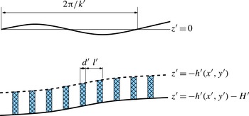
Referring to figure 1, we consider an idealized canopy formed by a periodic array of rigid cylinders of uniform height
 $H^{\prime }$
, diameter
 $d^{\prime }$
and spacing
 $l^{\prime }$
standing vertically on a seabed of slowly varying depth
 $h^{\prime }(x^{\prime },y^{\prime })$
. Distinguishing all dimensional quantities by primes, we let the canopy occupy the depth range
 $-H^{\prime }<z^{\prime }+h^{\prime }(x_{i}^{\prime })<0$
, where
 $h^{\prime }(x_{i}^{\prime })$
is the depth of the canopy top below the mean sea surface and
 $h_{0}^{\prime }=h^{\prime }+H^{\prime }$
is the total mean depth. Both
 $h^{\prime }$
and
 $h_{0}^{\prime }$
vary slowly in horizontal directions. The characteristic length of the passing waves is
 $2{\rm\pi}/k$
.
Definition sketch of a submerged canopy.

We shall assume that the flow above the canopy is incompressible and irrotational, and the wave amplitude is infinitesimal. The velocity potential
 ${\it\Phi}^{\prime }(x_{i}^{\prime },z^{\prime },t^{\prime })$
is governed by
 $$\begin{eqnarray}\frac{\partial ^{2}{\it\Phi}^{\prime }}{\partial x_{i}^{\prime }\partial x_{i}^{\prime }}+\frac{\partial ^{2}{\it\Phi}^{\prime }}{\partial {z^{\prime }}^{2}}=0,\quad i=1,2;~-h^{\prime }(x_{i}^{\prime })<z^{\prime }<0.\end{eqnarray}$$
The linearized free-surface condition reads
 $$\begin{eqnarray}\frac{\partial ^{2}{\it\Phi}^{\prime }}{\partial {t^{\prime }}^{2}}+g\frac{\partial {\it\Phi}^{\prime }}{\partial z^{\prime }}=0,\quad z^{\prime }=0.\end{eqnarray}$$
The canopy is a square array of identical cylinders, around each of which a unit cell can be defined. Let the cell average be
 $$\begin{eqnarray}\langle F^{\prime }\rangle ^{\prime }=\frac{1}{{\it\Omega}}\iint _{{\it\Omega}_{f}}F^{\prime }\text{d}x^{\prime }\text{d}y^{\prime },\end{eqnarray}$$
where
 ${\it\Omega}$
is the gross cross-sectional area of the cell and
 ${\it\Omega}_{f}$
is the fluid area within.
We now state the governing equations for the flow between cylinders. It is known from experiments on steady currents through emergent vegetation that flow separation leads to turbulence inside the canopy when
 $\mathit{Re}_{d}>200$
, where
 $\mathit{Re}_{d}=\langle U^{\prime }\rangle d^{\prime }/{\it\nu}$
is the Reynolds number and
 $\langle U^{\prime }\rangle$
the mean horizontal velocity and
 ${\it\nu}$
the molecular viscosity of water (Nepf Reference Nepf1999). An important aspect of the array is that the wake behind each cylinder is affected by turbulence originating from surrounding cylinders. In experiments on the flow around an isolated sphere in a steady current, Wu & Faeth (Reference Wu and Faeth1994a
) have examined the effect of free stream turbulence on the wake structure. Under the conditions of a particle Reynolds number of 135–1560, ambient turbulence intensities of 4 %, ratios of streamwise spatial integral scales to sphere diameters of 11–59 and ratios of Kolmogorov length scales to sphere diameters of 0.08–0.80, the turbulent wakes have mean streamwise velocities scaled like self-preserving laminar wakes if
 $\mathit{Re}_{d}<300$
and
 ${>}600$
, with enhanced eddy viscosities due to turbulence. Moreover, the eddy viscosity increases roughly linearly with the particle Reynolds number. Within the transitional range of
 $300<\mathit{Re}_{d}<600$
, wake oscillations and vortex shedding are prominent. These observations have been numerically confirmed by Bagchi & Balachandar (Reference Bagchi and Balachandar2004) for the range of
 $\mathit{Re}_{d}\leqslant 610$
using direct numerical simulation. Wu & Faeth (Reference Wu and Faeth1994b
) later extended the range of turbulence intensity in the free stream to 2 %–9.5 % for
 $125<\mathit{Re}_{d}<1560$
and found that wake oscillations and vortex shedding were suppressed when the free stream turbulence intensity exceeded 7 %. The wakes were similar to those seen in laminar flows. Now, in waves much longer than the cylinder spacing, each cylinder is in a turbulent environment caused not only by flow separation in its own wake but also by turbulence generated around its neighbours. It is reasonable to expect that the physics must be somewhat close to that of a steady turbulent current through a cylinder array. We shall therefore adopt the simple model of constant eddy viscosity and search for a reasonable way to determine its magnitude. This approach has been taken by Mei et al. (Reference Mei, Chan, Liu, Huang and Zhang2011), Mei et al. (Reference Mei, Chan and Liu2014) and Liu et al. (Reference Liu, Chang, Mei, Lomonaco, Martin and Maza2015) to yield macroscale predictions in reasonable agreement with experiments.
Accordingly, the mean flow inside the canopy is assumed to be governed by Reynolds equations with constant eddy viscosity
 ${\it\nu}_{t}$
. Let
 $u_{i}^{\prime },w^{\prime }$
denote the components of the fluid velocity between the cylinders inside the canopy. Incompressibility requires that
 $$\begin{eqnarray}\frac{\partial u_{i}^{\prime }}{\partial x_{i}^{\prime }}+\frac{\partial w^{\prime }}{\partial z^{\prime }}=0,\quad i=1,2;~-H^{\prime }<z^{\prime }+h^{\prime }(x_{i}^{\prime })<0.\end{eqnarray}$$
For infinitesimal waves the linearized momentum equations are
 $$\begin{eqnarray}\frac{\partial u_{i}^{\prime }}{\partial t^{\prime }}=-\frac{1}{{\it\rho}}\frac{\partial p^{\prime }}{\partial x_{i}^{\prime }}+{\it\nu}_{t}\left(\frac{\partial ^{2}u_{i}^{\prime }}{\partial x_{j}^{\prime }\partial x_{j}^{\prime }}+\frac{\partial ^{2}u_{i}^{\prime }}{\partial {z^{\prime }}^{2}}\right),\quad -H^{\prime }<z^{\prime }+h^{\prime }(x_{i}^{\prime })<0,\end{eqnarray}$$
where
 $i,j=1,2$
, and
 $$\begin{eqnarray}\frac{\partial w^{\prime }}{\partial t^{\prime }}=-\frac{1}{{\it\rho}}\frac{\partial p^{\prime }}{\partial z^{\prime }}+{\it\nu}_{t}\left(\frac{\partial ^{2}w^{\prime }}{\partial x_{j}^{\prime }\partial x_{j}^{\prime }}+\frac{\partial ^{2}w^{\prime }}{\partial {z^{\prime }}^{2}}\right),\quad -H^{\prime }<z^{\prime }+h^{\prime }(x_{i}^{\prime })<0,\end{eqnarray}$$
where
 $p^{\prime }$
denotes the dynamic pressure, so that the total pressure is
 $P^{\prime }=p^{\prime }-{\it\rho}gz^{\prime }$
. Determination of the eddy viscosity
 ${\it\nu}_{t}$
will be postponed until § 8 by equating the averaged work done by the force on the canopy and the rate of dissipation inside.
It is convenient to introduce a new vertical coordinate
 $z_{b}^{\prime }$
measured from the seabed,
 $$\begin{eqnarray}z_{b}^{\prime }=z^{\prime }+h^{\prime }(x_{i}^{\prime }),\end{eqnarray}$$
so that the canopy resides in
 $-H^{\prime }<z_{b}^{\prime }<0$
. The continuity equation becomes
 $$\begin{eqnarray}\frac{\partial u_{i}^{\prime }}{\partial x_{i}^{\prime }}+\frac{\partial h^{\prime }}{\partial x_{i}^{\prime }}\frac{\partial u_{i}^{\prime }}{\partial z_{b}^{\prime }}+\frac{\partial w^{\prime }}{\partial z_{b}^{\prime }}=0.\end{eqnarray}$$
The linearized momentum equations are changed to
 $$\begin{eqnarray}\displaystyle & \displaystyle \frac{\partial u_{i}^{\prime }}{\partial t^{\prime }}=-\frac{1}{{\it\rho}}\left(\frac{\partial }{\partial x_{i}^{\prime }}+\frac{\partial h^{\prime }}{\partial x_{i}^{\prime }}\frac{\partial }{\partial z_{b}^{\prime }}\right)p^{\prime }+{\it\nu}_{t}\left[\left(\frac{\partial }{\partial x_{j}^{\prime }}+\frac{\partial h^{\prime }}{\partial x_{j}^{\prime }}\frac{\partial }{\partial z_{b}^{\prime }}\right)^{2}u_{i}^{\prime }+\frac{\partial ^{2}u_{i}^{\prime }}{\partial {z_{b}^{\prime }}^{2}}\right],\quad i,j=1,2, & \displaystyle \nonumber\\ \displaystyle & & \displaystyle\end{eqnarray}$$
 $$\begin{eqnarray}\displaystyle & \displaystyle \frac{\partial w^{\prime }}{\partial t^{\prime }}=-\frac{1}{{\it\rho}}\frac{\partial p^{\prime }}{\partial z_{b}^{\prime }}+{\it\nu}_{t}\left[\left(\frac{\partial }{\partial x_{i}^{\prime }}+\frac{\partial h^{\prime }}{\partial x_{i}^{\prime }}\frac{\partial }{\partial z_{b}^{\prime }}\right)^{2}w^{\prime }+\frac{\partial ^{2}w^{\prime }}{\partial {z_{b}^{\prime }}^{2}}\right]. & \displaystyle\end{eqnarray}$$
In addition, we require no-slip on the sea bottom and the cylinder walls
 $S_{B}$
,
 $$\begin{eqnarray}u_{i}^{\prime }=w^{\prime }=0,\quad z_{b}^{\prime }=-H^{\prime }\quad \text{and}\quad (x_{i}^{\prime },z_{b}^{\prime })\in S_{B}.\end{eqnarray}$$
To be confirmed by experiments later, we ignore flow separation near the cylinder tips and assume that turbulence is primarily generated by shedding vortices around the cylinders. Hence, the tangential stress on the canopy top is neglected,
 $$\begin{eqnarray}{\it\tau}_{ij}^{\prime }n_{j}t_{i}=0,\quad z_{b}^{\prime }=0,\end{eqnarray}$$
where
 $\{n_{j}\}$
and
 $\{t_{i}\},~j=1,2,3$
, are respectively the unit normal and tangent vectors on the envelope of the canopy top. In addition, the cell-averaged normal velocity must be continuous,
 $$\begin{eqnarray}n_{x_{i}}\langle u_{i}^{\prime }\rangle ^{\prime }+n_{z}\langle w^{\prime }\rangle ^{\prime }=n_{x_{i}}\frac{\partial {\it\Phi}^{\prime }}{\partial x_{i}^{\prime }}+n_{z}\frac{\partial {\it\Phi}^{\prime }}{\partial z^{\prime }},\quad z^{\prime }=-h^{\prime }(x_{i}^{\prime }),\end{eqnarray}$$
where
 $\{n_{x_{i}},n_{z}\}$
is the unit normal vector on the envelope of the canopy top. Similarly, the cell-averaged inter-cylinder pressure
 $\langle \,p^{\prime }\rangle$
and the wave pressure must also be matched,
 $$\begin{eqnarray}-\!{\it\rho}\frac{\partial {\it\Phi}^{\prime }}{\partial t^{\prime }}=\langle \,p^{\prime }\rangle ^{\prime },\quad z^{\prime }=-h^{\prime }(x_{i}^{\prime }).\end{eqnarray}$$
3. Normalization
In the canopy, there are three distinct length scales: the microscale represented by the spacing
 $\ell ^{\prime }$
between cylinders, the much greater mesoscale
 $1/k_{0}^{\prime }=g/{\it\omega}^{\prime 2}$
characterizing the wave motion, and the still much greater macroscale
 $L^{\prime }$
characterizing the horizontal variation of bathymetry and the extent of the canopy. Let all normalized variables be denoted by plain symbols, and the small parameter
 ${\it\epsilon}\equiv k_{0}^{\prime }\ell ^{\prime }\ll 1$
be the measure of length contrast between the scales. We define the following triad of micro- (
 ${\it\xi}_{i},{\it\zeta}$
), meso- (
 $x_{i},z$
) and macro- (
 $X_{i}$
) coordinates:
 $$\begin{eqnarray}\left\{{\it\xi}_{i}=\frac{x_{i}^{\prime }}{\ell ^{\prime }}=\frac{x_{i}}{{\it\epsilon}},{\it\zeta}=\frac{(z^{\prime }+h^{\prime })}{\ell ^{\prime }}=\frac{z_{b}}{{\it\epsilon}}\right\}\!,\quad \left\{x_{i}=k_{0}^{\prime }x_{i}^{\prime },~z=k_{0}^{\prime }z^{\prime }\right\}\!,\quad X_{i}={\it\epsilon}x_{i}={\it\epsilon}^{2}{\it\xi}_{i}.\end{eqnarray}$$
Let the incoming wave amplitude be
 $A_{0}^{\prime }$
. We also define the dimensionless variables for the inter-cylinder flow as follows:
 $$\begin{eqnarray}t={\it\omega}^{\prime }t^{\prime },\quad u_{i}=\frac{u_{i}^{\prime }}{{\it\omega}^{\prime }A_{0}^{\prime }}=\frac{{\it\omega}^{\prime }}{gk_{0}^{\prime }A_{0}^{\prime }}u_{i}^{\prime },\quad w=\frac{1}{k_{0}^{\prime }\ell ^{\prime }}\frac{w^{\prime }}{{\it\omega}^{\prime }A_{0}^{\prime }},\quad p=\frac{p^{\prime }}{{\it\rho}gA_{0}^{\prime }},\end{eqnarray}$$
and assume
 $$\begin{eqnarray}H=\frac{H^{\prime }}{\ell ^{\prime }}=O(1),\quad h=k_{0}^{\prime }h^{\prime }=O(1).\end{eqnarray}$$
The normalized equations of continuity, horizontal and vertical momentum are respectively
 $$\begin{eqnarray}\displaystyle & \displaystyle \frac{\partial u_{i}}{\partial {\it\xi}_{i}}+{\it\epsilon}\frac{\partial h}{\partial X_{i}}\frac{\partial u_{i}}{\partial {\it\zeta}}+{\it\epsilon}\frac{\partial w}{\partial {\it\zeta}}=0,\quad -H<{\it\zeta}<0, & \displaystyle\end{eqnarray}$$
 $$\begin{eqnarray}\displaystyle & \displaystyle {\it\epsilon}\frac{\partial u_{i}}{\partial t}=-\!\left(\frac{\partial p}{\partial {\it\xi}_{i}}+{\it\epsilon}\frac{\partial h}{\partial X_{i}}\frac{\partial p}{\partial {\it\zeta}}\right)+{\it\epsilon}{\it\sigma}\left[\left(\frac{\partial }{\partial {\it\xi}_{j}}+{\it\epsilon}\frac{\partial h}{\partial X_{j}}\frac{\partial }{\partial {\it\zeta}}\right)^{2}u_{i}+\frac{\partial ^{2}u_{i}}{\partial {\it\zeta}^{2}}\right],\quad -H<{\it\zeta}<0, & \displaystyle \nonumber\\ \displaystyle & & \displaystyle\end{eqnarray}$$
 $$\begin{eqnarray}\displaystyle & \displaystyle {\it\epsilon}^{2}\frac{\partial w}{\partial t}=-\frac{\partial p}{\partial {\it\zeta}}+{\it\epsilon}^{2}{\it\sigma}\left[\left(\frac{\partial }{\partial {\it\xi}_{j}}+{\it\epsilon}\frac{\partial h}{\partial X_{j}}\frac{\partial }{\partial {\it\zeta}}\right)^{2}w+\frac{\partial ^{2}w}{\partial {\it\zeta}^{2}}\right],\quad -H<{\it\zeta}<0, & \displaystyle\end{eqnarray}$$
 $$\begin{eqnarray}{\it\sigma}=\frac{{\it\nu}_{t}}{{\it\omega}^{\prime }{\ell ^{\prime }}^{2}}\end{eqnarray}$$
denotes the dimensionless eddy viscosity. As it is a property of the flow, we regard
 ${\it\sigma}$
to be of arbitrary order-of-magnitude relative to the geometrical parameter
 ${\it\epsilon}$
. The boundary conditions on the seabed and the cylinder walls become
 $$\begin{eqnarray}u_{i}=w=0,\quad {\it\zeta}=-H\quad \text{and}\quad ({\it\xi}_{i},{\it\zeta})\in S_{B}.\end{eqnarray}$$
It should be noted that these equations are normalized by the microlength
 $\ell ^{\prime }$
, and hence can describe variations inside the cells.
In the irrotational zone outside the canopy, we normalize the potential as
 $$\begin{eqnarray}{\it\Phi}={\it\Phi}^{\prime }\frac{{\it\omega}^{\prime }}{gA_{0}^{\prime }}.\end{eqnarray}$$
The mesoscale variation is governed by
 $$\begin{eqnarray}\frac{\partial ^{2}{\it\Phi}}{\partial x_{i}\partial x_{i}}+\frac{\partial ^{2}{\it\Phi}}{\partial z^{2}}=0,\quad -h<z<0,\end{eqnarray}$$
and
 $$\begin{eqnarray}\frac{\partial {\it\Phi}}{\partial z}+\frac{\partial ^{2}{\it\Phi}}{\partial t^{2}}=0,\quad z=0.\end{eqnarray}$$
Let the slow variation of sea depth be expressed by
 $h(X_{i})$
. On the canopy top, (2.13) becomes
 $$\begin{eqnarray}n_{i}\langle u_{i}\rangle +{\it\epsilon}n_{z}\langle w\rangle =n_{i}\frac{\partial {\it\Phi}}{\partial x_{i}}+n_{z}\frac{\partial {\it\Phi}}{\partial z},\quad z=-h(X_{i}),\end{eqnarray}$$
where
 $(n_{i},n_{z})$
are components of the unit normal vector, and
 $$\begin{eqnarray}-\!\frac{\partial {\it\Phi}}{\partial t}=\langle \,p\rangle ,\quad z=-h(X_{i}),\end{eqnarray}$$
where
 $$\begin{eqnarray}\langle G\rangle \equiv \iint _{~{\it\Omega}_{f}}G\text{d}{\it\xi}_{1}\text{d}{\it\xi}_{2}.\end{eqnarray}$$
4. Depth-averaged equations for canopy flow
Let us denote the vertical averages over the canopy height by tildes,
 $$\begin{eqnarray}\widetilde{F}=\frac{1}{H}\int _{-H}^{0}F\text{d}{\it\zeta}.\end{eqnarray}$$
We obtain from the continuity equation
 $$\begin{eqnarray}\frac{\partial \widetilde{u}_{i}}{\partial {\it\xi}_{i}}+\frac{{\it\epsilon}}{H}\left[\frac{\partial h}{\partial X_{i}}u_{i}+w\right]_{{\it\zeta}=-H}^{{\it\zeta}=0}=\frac{\partial \widetilde{u}_{i}}{\partial {\it\xi}_{i}}+\frac{{\it\epsilon}}{H}\left[\frac{\partial h}{\partial X_{i}}u_{i}+w\right]_{{\it\zeta}=0}=0.\end{eqnarray}$$
The depth-averaged horizontal momentum equation (3.5) is
 $$\begin{eqnarray}\displaystyle {\it\epsilon}\frac{\partial \widetilde{u}_{i}}{\partial t}=-\!\left(\frac{\partial \widetilde{p}}{\partial {\it\xi}_{i}}+{\it\epsilon}\frac{\partial h}{\partial X_{i}}\frac{1}{H}\int _{-H}^{0}\text{d}{\it\zeta}\,\frac{\partial p}{\partial {\it\zeta}}\right)+{\it\epsilon}{\it\sigma}\left[\left(\frac{\partial }{\partial {\it\xi}_{j}}+{\it\epsilon}\frac{\partial h}{\partial X_{j}}\frac{\partial }{\partial {\it\zeta}}\right)^{2}\widetilde{u}_{i}+\frac{1}{H}\left[\frac{\partial u_{i}}{\partial {\it\zeta}}\right]_{-H}^{0}\right]. & & \displaystyle \nonumber\\ \displaystyle & & \displaystyle\end{eqnarray}$$
The vertical momentum equation (3.6) implies hydrostatic pressure,
 $$\begin{eqnarray}\frac{\partial p}{\partial {\it\zeta}}=O({\it\epsilon}^{2}).\end{eqnarray}$$
Since
 ${\it\epsilon}h_{X_{i}}=O({\it\epsilon})$
is equal to the seabed slope and is small, it is easy to show that
 $(n_{i},t_{z})=O({\it\epsilon}),(n_{z},t_{i})=1+O({\it\epsilon}^{2})$
, where
 $(t_{i},t_{z})$
are components of the unit tangent vector to the seabed. The condition of vanishing shear stress on the canopy top gives, to the leading order,
 $$\begin{eqnarray}\frac{\partial u_{i}}{\partial {\it\zeta}}=O({\it\epsilon}^{2}),\quad {\it\zeta}=0.\end{eqnarray}$$
We assume for simplicity that the bottom shear stress is a linear function of the tangential velocity with an empirical factor
 ${\it\beta}$
,
 $$\begin{eqnarray}\frac{{\it\sigma}}{H}\frac{\partial u_{i}}{\partial {\it\zeta}}={\it\beta}\widetilde{u}_{i},\quad {\it\zeta}=-H.\end{eqnarray}$$
Ignoring small terms of
 $O({\it\epsilon}^{2})$
, the depth-averaged horizontal momentum equation is reduced to
 $$\begin{eqnarray}{\it\epsilon}\frac{\partial \widetilde{u}_{i}}{\partial t}=-\frac{\partial \widetilde{p}}{\partial {\it\xi}_{i}}+{\it\epsilon}{\it\sigma}\frac{\partial ^{2}\widetilde{u}_{i}}{\partial {\it\xi}_{j}\partial {\it\xi}_{j}}-{\it\epsilon}{\it\beta}\widetilde{u}_{i}.\end{eqnarray}$$
In the literature on coastal processes it is usual to model the bed stress by a quadratic law, which can be quasi-linearized for analytical convenience to
 $$\begin{eqnarray}\frac{{\it\tau}_{w}^{\prime }}{{\it\rho}}={\it\nu}_{t}\frac{\partial u^{\prime }}{\partial z^{\prime }}=\frac{f_{w}}{2}\frac{8}{3{\rm\pi}}|\widetilde{u}_{max}^{\prime }|\widetilde{u}^{\prime },\quad z^{\prime }=-h_{0}^{\prime },\end{eqnarray}$$
where
 $f_{w}$
is the friction factor related empirically to the bottom roughness and
 $|\widetilde{u}_{max}^{\prime }|$
is the amplitude of the time-periodic velocity at the bottom (see Mei (Reference Mei1989, p. 262) or Mei, Stiassnie & Yue (Reference Mei, Stiassnie and Yue2005, p. 285)). In normalized form, we have
 $$\begin{eqnarray}\frac{{\it\sigma}}{H}\frac{\partial u}{\partial {\it\zeta}}=\frac{f_{w}}{2}\left(\frac{A_{0}^{\prime }}{H^{\prime }}|\widetilde{u}_{max}|\right)\widetilde{u},\quad \text{hence}~{\it\beta}=\frac{4f_{w}}{3{\rm\pi}}\frac{A_{0}^{\prime }}{H^{\prime }}|\widetilde{u}_{max}|.\end{eqnarray}$$
The boundary conditions on the cylinder surface remain
 $$\begin{eqnarray}\widetilde{u}_{i}=\widetilde{w}=0,\quad ({\it\xi}_{i},{\it\zeta})\in S_{B}.\end{eqnarray}$$
5. Homogenization analysis of canopy flow
To consider the multiscaled variation of the flow we introduce the expansions
 $$\begin{eqnarray}\displaystyle & u_{i}=u_{i}^{(0)}+{\it\epsilon}u_{i}^{(1)}+{\it\epsilon}^{2}u_{i}^{(2)}+\cdots \,, & \displaystyle\end{eqnarray}$$
 $$\begin{eqnarray}\displaystyle & w=w^{(0)}+{\it\epsilon}w^{(1)}+\cdots \,, & \displaystyle\end{eqnarray}$$
 $$\begin{eqnarray}\displaystyle & p=p^{(0)}+{\it\epsilon}p^{(1)}+{\it\epsilon}^{2}p^{(2)}+\cdots \,, & \displaystyle\end{eqnarray}$$
 $({\it\xi}_{i},x_{i},X_{i},z,t)$
with
 $x_{i}={\it\epsilon}{\it\xi}_{i},X_{i}={\it\epsilon}x_{i}={\it\epsilon}^{2}{\it\xi}_{i}$
. The depth averages
 $\widetilde{u}_{i},\widetilde{p}$
are similarly expanded. By substituting these into the governing equations we obtain the perturbation equations for the microscale variations in a typical cell
 ${\it\Omega}$
. Within each cell, the continuity equation (4.2) requires
 $$\begin{eqnarray}\frac{\partial \widetilde{u}_{i}^{(0)}}{\partial {\it\xi}_{i}}+{\it\epsilon}\frac{\partial \widetilde{u}_{i}^{(0)}}{\partial x_{i}}+{\it\epsilon}\frac{\partial \widetilde{u}_{i}^{(1)}}{\partial {\it\xi}_{i}}+\frac{{\it\epsilon}}{H}\left[\frac{\partial h}{\partial X_{i}}u_{i}^{(0)}+w^{(0)}\right]_{{\it\zeta}=0}=O({\it\epsilon}^{2}).\end{eqnarray}$$
Hence, we have at
 $O(1)$
,
 $$\begin{eqnarray}\frac{\partial \widetilde{u}_{i}^{(0)}}{\partial {\it\xi}_{i}}=0,\quad {\it\xi}_{i}\in {\it\Omega}.\end{eqnarray}$$
Taking the cell average of the
 $O({\it\epsilon})$
part of (5.4), we obtain
 $$\begin{eqnarray}\frac{\partial \langle \widetilde{u}_{i}^{(0)}\rangle }{\partial x_{i}}+\iint _{\,{\it\Omega}_{f}}\frac{\partial \widetilde{u}_{i}^{(1)}}{\partial {\it\xi}_{i}}\text{d}{\it\xi}_{1}\text{d}{\it\xi}_{2}+\frac{1}{H}\left[\langle w^{(0)}\rangle +\langle u_{i}^{(0)}\rangle \frac{\partial h}{\partial X_{i}}\right]_{{\it\zeta}=0}=0.\end{eqnarray}$$
By using Gauss’ theorem and requiring that physical unknowns are cell-periodic, the double integral vanishes so that
 $$\begin{eqnarray}\langle w^{(0)}\rangle +\langle u_{i}^{(0)}\rangle \frac{\partial h}{\partial X_{i}}=-H\frac{\partial \langle \widetilde{u}_{i}^{(0)}\rangle }{\partial x_{i}},\quad {\it\zeta}=0.\end{eqnarray}$$
Physically, the net horizontal flux across the side boundaries of the cell leads to a normal flux on the cell top. This result will be used later as a boundary condition for the irrotational flow above.
The horizontal momentum equation (4.3) is expanded as
 $$\begin{eqnarray}{\it\epsilon}\frac{\partial \widetilde{u}_{i}^{(0)}}{\partial t}=-\frac{\partial \widetilde{p}^{(0)}}{\partial {\it\xi}_{i}}-{\it\epsilon}\frac{\partial h}{\partial X_{i}}\frac{\partial \widetilde{p}^{(0)}}{\partial {\it\zeta}}-{\it\epsilon}\frac{\partial \widetilde{p}^{(1)}}{\partial {\it\xi}_{i}}-{\it\epsilon}\frac{\partial \widetilde{p}^{(0)}}{\partial x_{i}}+{\it\epsilon}{\it\sigma}\frac{\partial ^{2}\widetilde{u}_{i}^{(0)}}{\partial {\it\xi}_{k}\partial {\it\xi}_{k}}-{\it\epsilon}{\it\beta}\widetilde{u}_{i}^{(0)}+O({\it\epsilon}^{2}).\end{eqnarray}$$
Because of (4.4), the leading-order pressure is independent of the microscale
 ${\it\xi}_{i}$
and
 ${\it\zeta}$
,
 $$\begin{eqnarray}p^{(0)}=\widetilde{p}^{(0)}=\widetilde{p}^{(0)}(x_{i},X_{i},t).\end{eqnarray}$$
Equation (5.8) now reads
 $$\begin{eqnarray}\frac{\partial \widetilde{u}_{i}^{(0)}}{\partial t}=-\frac{\partial p^{(1)}}{\partial {\it\xi}_{i}}-\frac{\partial p^{(0)}}{\partial x_{i}}+{\it\sigma}\frac{\partial \widetilde{u}_{i}^{(0)}}{\partial {\it\xi}_{j}\partial {\it\xi}_{j}}-{\it\beta}\widetilde{u}_{i}^{(0)},\quad {\it\xi}_{i}\in {\it\Omega}.\end{eqnarray}$$
For given
 ${\it\nu}_{t}$
or
 ${\it\sigma}$
, the leading-order dynamics in a typical cell must be solved from (5.5) and (5.10), as explained below.
6. Cell problem and canopy permeability
Consider more specifically simple harmonic waves of frequency
 ${\it\omega}$
so that all dimensionless unknowns are proportional to
 $\text{e}^{-\text{i}t}$
. Denoting the complex amplitudes by upper-case letters, i.e.
 $$\begin{eqnarray}(\widetilde{u}_{i}^{(0)},\widetilde{w}^{(0)},\widetilde{p}^{(0)},\widetilde{p}^{(1)})=\text{Re}[(U_{i}^{(0)},W^{(0)},P^{(0)},P^{(1)})\text{e}^{-\text{i}t}],\end{eqnarray}$$
where the spatial amplitudes
 $U^{(0)},P^{(0)},P^{(1)}$
are functions of (
 ${\it\xi}_{1},{\it\xi}_{2}$
) but not of
 ${\it\zeta}$
, all equations in § 5 still hold for the spatial factors, except that
 $\partial \widetilde{u}_{i}^{(0)}/\partial t$
is replaced by
 $-\text{i}U_{i}^{(0)}$
in (5.10).
Due to linearity, the factors
 $U_{i}^{(0)}$
and
 $P^{(1)}$
are proportional to the macroscale pressure gradient
 $\partial P^{(0)}/\partial X_{j}$
. Hence, we assume
 $$\begin{eqnarray}U_{i}^{(0)}=-\unicode[STIX]{x1D612}_{ij}\frac{\partial P^{(0)}}{\partial X_{j}},\quad P^{(1)}=-B_{j}\frac{\partial P^{(0)}}{\partial X_{j}}.\end{eqnarray}$$
From (5.5) and (5.10),
 $\unicode[STIX]{x1D612}_{ij}({\it\xi}_{k})$
and
 $B_{j}({\it\xi}_{k})$
must satisfy the following equations in an
 ${\it\Omega}$
-cell on the microscale:
 $$\begin{eqnarray}\displaystyle & \displaystyle \frac{\partial \unicode[STIX]{x1D612}_{ij}}{\partial {\it\xi}_{j}}=0,\quad {\it\xi}_{i}\in {\it\Omega}, & \displaystyle\end{eqnarray}$$
 $$\begin{eqnarray}\displaystyle & \displaystyle -\text{i}\unicode[STIX]{x1D612}_{ij}={\it\delta}_{ij}-\frac{\partial B_{i}}{\partial {\it\xi}_{j}}+{\it\sigma}\frac{\partial ^{2}\unicode[STIX]{x1D612}_{ij}}{\partial {\it\xi}_{k}\partial {\it\xi}_{k}}-{\it\beta}\unicode[STIX]{x1D612}_{ij},\quad {\it\xi}_{k}\in {\it\Omega}. & \displaystyle\end{eqnarray}$$
 $$\begin{eqnarray}\unicode[STIX]{x1D612}_{ij},B_{j}:{\it\Omega}\text{-periodic}\end{eqnarray}$$
and no-slip on cylinder walls:
 $$\begin{eqnarray}\unicode[STIX]{x1D612}_{ij}=0,\quad {\it\xi}_{k}\in S_{B}.\end{eqnarray}$$
For uniqueness we also impose
 $$\begin{eqnarray}\langle B_{j}\rangle =0.\end{eqnarray}$$
It should be noted that
 $\unicode[STIX]{x1D612}_{ij}$
may depend on
 $x_{i}$
and
 $X_{i}$
indirectly through
 ${\it\nu}_{t}$
or
 ${\it\sigma}$
.
With a trial value for
 ${\it\sigma}$
, the canonical cell problem for
 $\unicode[STIX]{x1D612}_{ij}$
and
 $B_{j}$
can be solved by the standard method of finite elements, as in Mei et al. (Reference Mei, Chan, Liu, Huang and Zhang2011). In this work nine-node triangular cubic elements are used. The total matrix for the nodal coefficients is sparse and is solved by LU decomposition. Approximately 3000 elements are used in the unit cell with 100 element cells along the cylinder surface, which can ensure a converged numerical solution.
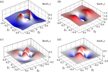
For a square cell enclosing one circular cylinder, sample distributions of
 $\unicode[STIX]{x1D612}_{ij}$
are shown in figure 2. The cell-averaged value
 $\langle \unicode[STIX]{x1D612}_{21}\rangle$
is zero as expected.
Sample distribution of
 $\unicode[STIX]{x1D612}_{ij}$
in a unit cell. The input parameters are
 $n=0.95$
,
 ${\it\sigma}=3.0\times 10^{-3}$
and
 ${\it\beta}=0$
.

The cell averages of (6.2) give the dynamic Darcy’s law
 $$\begin{eqnarray}\langle U_{i}^{(0)}\rangle =-\langle \unicode[STIX]{x1D612}_{ij}\rangle \frac{\partial P^{(0)}}{\partial x_{j}},\quad -H<{\it\zeta}<0,\end{eqnarray}$$
where
 $\langle \unicode[STIX]{x1D612}_{ij}\rangle$
is the normalized complex permeability tensor, related to the dimensional permeability by
 $\langle \unicode[STIX]{x1D612}_{ij}\rangle =\langle \unicode[STIX]{x1D612}_{ij}^{\prime }\rangle /{\it\rho}{\it\omega}^{\prime }$
. It should be noted that
 $$\begin{eqnarray}\langle P^{(1)}\rangle =-\langle B_{j}\rangle \frac{\partial P^{(0)}}{\partial x_{j}}=0,\end{eqnarray}$$
hence
 $P^{(0)}$
represents the cell-averaged dynamic pressure with an error of
 $O({\it\epsilon}^{2})$
.
In view of (6.2) and (3.13), (5.7) becomes
 $$\begin{eqnarray}\langle W^{(0)}\rangle +\langle U_{i}^{(0)}\rangle \frac{\partial h}{\partial X_{i}}=H\frac{\partial }{\partial x_{i}}\left(\langle \unicode[STIX]{x1D612}_{ij}\rangle \frac{\partial P^{(0)}}{\partial x_{j}}\right)=\text{i}H\frac{\partial }{\partial x_{i}}\left(\langle \unicode[STIX]{x1D612}_{ij}\rangle \frac{\partial {\it\phi}}{\partial x_{j}}\right),\quad {\it\zeta}=0.\end{eqnarray}$$
7. Waves above an isotropic canopy
Consider simple harmonic waves
 $$\begin{eqnarray}{\it\Phi}=\text{Re}({\it\phi}\text{e}^{-\text{i}t}).\end{eqnarray}$$
For general two-dimensional bathymetry, the boundary-value problem for
 ${\it\phi}$
is governed by (3.10) and
 $$\begin{eqnarray}\frac{\partial {\it\phi}}{\partial z}-{\it\phi}=0,\quad z=0.\end{eqnarray}$$
To enforce the continuity of normal velocity at the top of the canopy, we first let
 $$\begin{eqnarray}{\it\phi}={\it\phi}^{(0)}+{\it\epsilon}{\it\phi}^{(1)}+\cdots\end{eqnarray}$$
and then use
 $\partial h/\partial x_{i}={\it\epsilon}(\partial h/\partial X_{i})$
,
 $n_{i}={\it\epsilon}(\partial h/\partial X_{i})+O({\it\epsilon}^{2})$
,
 $n_{z}=1+O({\it\epsilon}^{2})$
, to obtain from (3.12)
 $$\begin{eqnarray}\displaystyle \frac{\partial {\it\phi}}{\partial z}+{\it\epsilon}\frac{\partial h}{\partial X_{j}}\frac{\partial {\it\phi}}{\partial x_{j}} & = & \displaystyle {\it\epsilon}\frac{\partial h}{\partial X_{j}}\left(\frac{\partial {\it\phi}^{(0)}}{\partial x_{j}}+{\it\epsilon}\frac{\partial {\it\phi}^{(1)}}{\partial x_{j}}+\cdots \right)+\frac{\partial {\it\phi}^{(0)}}{\partial z}+{\it\epsilon}\frac{\partial {\it\phi}^{(1)}}{\partial z}+\cdots \nonumber\\ \displaystyle & = & \displaystyle {\it\epsilon}\frac{\partial h}{\partial X_{j}}\langle U_{j}^{(0)}\rangle +{\it\epsilon}\langle W^{(0)}\rangle +O({\it\epsilon}^{2}),\quad z=-h,\end{eqnarray}$$
which can be rewritten as
 $$\begin{eqnarray}\frac{\partial {\it\phi}}{\partial z}+{\it\epsilon}\frac{\partial h}{\partial X_{j}}\frac{\partial {\it\phi}}{\partial x_{j}}=\text{i}{\it\epsilon}H\frac{\partial }{\partial x_{i}}\left(\langle \unicode[STIX]{x1D612}_{ij}\rangle \frac{\partial {\it\phi}}{\partial x_{j}}\right)+O({\it\epsilon}^{2}),\quad z=-h,\end{eqnarray}$$
after using (6.10) on the right-hand side.
From here on we shall restrict our attention to the special case of an isotropic and uniform canopy,
 $\langle \unicode[STIX]{x1D612}_{ij}\rangle =\mathscr{K}{\it\delta}_{ij}$
. It will be shown later that for slowly varying depth,
 $\mathscr{K}(X_{i})$
also varies slowly in horizontal directions. Thus we have
 $$\begin{eqnarray}\frac{\partial {\it\phi}}{\partial z}=-{\it\epsilon}\frac{\partial h}{\partial X_{j}}\frac{\partial {\it\phi}}{\partial x_{j}}+\text{i}{\it\epsilon}\mathscr{K}H\frac{\partial ^{2}{\it\phi}}{\partial x_{j}^{2}}+O({\it\epsilon}^{2}),\quad z=-h.\end{eqnarray}$$
As a check, the limit of no canopy corresponds to
 $\text{i}\mathscr{K}=-1$
from (6.4). Equation (7.6) reduces to
 $$\begin{eqnarray}\frac{\partial {\it\phi}}{\partial z}=-{\it\epsilon}\frac{\partial h}{\partial X_{j}}\frac{\partial {\it\phi}}{\partial x_{j}}-{\it\epsilon}H\frac{\partial ^{2}{\it\phi}}{\partial x_{j}^{2}}=-{\it\epsilon}\frac{\partial h}{\partial X_{j}}\frac{\partial {\it\phi}}{\partial x_{j}}+{\it\epsilon}H\frac{\partial ^{2}{\it\phi}}{\partial z^{2}},\quad z=-h,\end{eqnarray}$$
which is the small-
 ${\it\epsilon}$
approximation of the exact no-flux boundary condition on
 $z=-h_{o}$
,
 $$\begin{eqnarray}\frac{\partial {\it\phi}}{\partial z}=-{\it\epsilon}\frac{\partial h}{\partial X_{j}}\frac{\partial {\it\phi}}{\partial x_{j}},\quad z=-h_{o}=-h-{\it\epsilon}H,\end{eqnarray}$$
by Taylor expansion.
The slow evolution of waves is governed by (3.10), (7.2) and (7.6), and can be treated by the known method of ray (Wentzel–Kramers–Brillouin) approximation (see e.g. Mei Reference Mei1989 and Mei et al. Reference Mei, Stiassnie and Yue2005), as sketched below.
First, we assume the expansion
 $$\begin{eqnarray}{\it\phi}=\left[{\it\psi}^{(0)}(X_{j},z)+(-\text{i}{\it\epsilon}){\it\psi}^{(1)}(X_{j},z)+(-\text{i}{\it\epsilon})^{2}{\it\psi}^{(2)}(X_{j},z)+\cdots \right]\text{e}^{\text{i}S/{\it\epsilon}}\end{eqnarray}$$
where
 $S(X_{j})$
is the wave phase. Denoting
 $\boldsymbol{{\rm\nabla}}=(\partial _{x},\partial _{y})$
and
 $\widehat{\boldsymbol{{\rm\nabla}}}=(\partial _{X},\partial _{Y})$
, we define the wavenumber vector by
 $\boldsymbol{k}(X_{j})=\widehat{\boldsymbol{{\rm\nabla}}}S=\boldsymbol{{\rm\nabla}}S/{\it\epsilon}$
, with
 $\boldsymbol{{\rm\nabla}}={\it\epsilon}\widehat{\boldsymbol{{\rm\nabla}}}$
and
 $k=|\boldsymbol{k}|$
.
At
 $O(1)$
the boundary-value problem for
 ${\it\psi}^{(0)}$
is homogeneous and has the formal solution
 $$\begin{eqnarray}{\it\psi}^{(0)}=-\text{i}A(X_{j})\frac{\cosh k(z+h)}{\cosh kh},\end{eqnarray}$$
where
 $$\begin{eqnarray}1=k\tanh kh\end{eqnarray}$$
is the dimensionless dispersion relation. Together with
 $$\begin{eqnarray}\widehat{\boldsymbol{{\rm\nabla}}}\times \boldsymbol{k}=0,\end{eqnarray}$$
the wavenumber vector
 $\boldsymbol{k}$
can be determined. The dimensionless wave amplitude
 $A(X_{j})$
is found from the solvability condition of
 ${\it\psi}^{(1)}$
governed by the inhomogeneous boundary-value problem at
 $O({\it\epsilon})$
,
 $$\begin{eqnarray}\displaystyle & \displaystyle \frac{\partial ^{2}{\it\psi}^{(1)}}{\partial z^{2}}-k^{2}{\it\psi}^{(1)}=\boldsymbol{k}\boldsymbol{\cdot }\widehat{\boldsymbol{{\rm\nabla}}}{\it\psi}^{(0)}+\widehat{\boldsymbol{{\rm\nabla}}}\boldsymbol{\cdot }(\boldsymbol{k}{\it\psi}^{(0)}),\quad -h<z<0, & \displaystyle\end{eqnarray}$$
 $$\begin{eqnarray}\displaystyle & \displaystyle \frac{\partial {\it\psi}^{(1)}}{\partial z}-{\it\psi}^{(1)}=0,\quad z=0, & \displaystyle\end{eqnarray}$$
 $$\begin{eqnarray}\displaystyle & \displaystyle \frac{\partial {\it\psi}^{(1)}}{\partial z}=(\boldsymbol{k}\boldsymbol{\cdot }\widehat{\boldsymbol{{\rm\nabla}}}h){\it\psi}^{(0)}+\mathscr{K}k^{2}H{\it\psi}^{(0)}\quad z=-h. & \displaystyle\end{eqnarray}$$
 ${\it\psi}^{(0)}$
and
 ${\it\psi}^{(1)}$
and performing partial integrations we obtain
 $$\begin{eqnarray}\widehat{\boldsymbol{{\rm\nabla}}}\boldsymbol{\cdot }\int _{-h}^{0}\text{d}z\,\boldsymbol{k}({\it\psi}^{(0)})^{2}=-\!\left(\mathscr{K}k^{2}H\right)({\it\psi}^{(0)})_{z=-h}^{2}.\end{eqnarray}$$
It follows after using (7.10) and (7.11) that
 $$\begin{eqnarray}\widehat{\boldsymbol{{\rm\nabla}}}\boldsymbol{\cdot }\left(\boldsymbol{C}_{g}A^{2}\right)=-A^{2}\frac{k^{2}H}{\cosh ^{2}kh}\mathscr{K},\end{eqnarray}$$
where
 $\boldsymbol{C}_{g}=C_{g}\boldsymbol{k}/k$
is the dimensionless group velocity
 $$\begin{eqnarray}C_{g}=\frac{1}{2k}\left(1+\frac{2kh}{\sinh 2kh}\right),\end{eqnarray}$$
which is related to the dimensional group velocity by
 $C_{g}=(g/{\it\omega})C_{g}^{\prime }$
.
Let
 $A=|A|\text{e}^{\text{i}{\it\theta}}$
in (7.17), and eliminate
 $\text{e}^{2\text{i}{\it\theta}}$
. We obtain from the real part the variation of wave energy
 $$\begin{eqnarray}\widehat{\boldsymbol{{\rm\nabla}}}\boldsymbol{\cdot }\left(\boldsymbol{C}_{g}|A|^{2}\right)=-|A|^{2}\frac{k^{2}H}{\cosh ^{2}kh}\text{Re}(\mathscr{K}),\end{eqnarray}$$
which can be integrated numerically along the rays. From the imaginary part, the change of wave phase is
 $$\begin{eqnarray}{\it\epsilon}\frac{\boldsymbol{k}}{k}\boldsymbol{\cdot }\widehat{\boldsymbol{{\rm\nabla}}}{\it\theta}=-\frac{{\it\epsilon}k^{2}H}{2C_{g}\cosh ^{2}kh}\text{Im}(\mathscr{K})=-\frac{{\it\epsilon}}{C_{g}}\frac{kH}{\sinh 2kh}\text{Im}(\mathscr{K}).\end{eqnarray}$$
Thus, the geometry of rays is also changed by the presence of the canopy.
Numerical computations will be carried out later only for the special case of normal incidence over one-dimensional bathymetry,
 $\partial /\partial Y=0$
. We then have simply
 $$\begin{eqnarray}C_{g}|A|^{2}=\left(C_{g}|A|^{2}\right)_{0}\exp \left\{-\int _{0}^{X}\text{d}X\,\left[\frac{1}{C_{g}}\frac{2kH}{\sinh 2kh}\text{Re}(\mathscr{K})\right]\right\}.\end{eqnarray}$$
Thus, the wave energy
 $C_{g}|A|^{2}$
decays exponentially along the canopy.
In the limit of no canopy, the clear-water depth is
 $h_{o}=h+H$
and
 $\mathscr{K}=i$
, hence
 $\text{Re}(\mathscr{K})=0,\text{Im}(\mathscr{K})=1$
. Equation (7.21) gives
 $C_{g}|A|^{2}=[C_{g}|A|^{2}]_{0}$
, as is well known. The phase change is
 $$\begin{eqnarray}{\rm\Delta}k={\it\epsilon}\frac{\partial {\it\theta}}{\partial X}=-\frac{{\it\epsilon}}{C_{g}}\frac{kH}{\sinh 2kh}=-\frac{{\it\epsilon}}{C_{g}}\frac{k^{2}H}{2\cosh ^{2}kh}=O({\it\epsilon}),\end{eqnarray}$$
which ensures that
 $k+{\rm\Delta}k$
and
 $h+H$
satisfy the classical dispersion relation
 $$\begin{eqnarray}1=(k+{\rm\Delta}k)\tanh \left((k+{\rm\Delta}k)(h+H)\right)\end{eqnarray}$$
within the error of
 $O({\it\epsilon}^{2})$
. This limit is well known in the classical theory of infinitesimal waves. Experimental confirmation including the second-order effects of set-down and set-up can be found in Bowen, Inman & Simmons (Reference Bowen, Inman and Simmons1968).
Equations (7.21) and (7.20) must be numerically integrated by quadrature for given
 $h(X)$
.
We now turn to the determination of the eddy viscosity.
8. Determination of the eddy viscosity
For steady flows through emergent vegetation, Nepf (Reference Nepf1999) determined the eddy viscosity and the eddy diffusivity of momentum (and mass) by requiring that the work done by the drag force on a cell be equal to the energy dissipation in the cell. By order-of-magnitude estimates of the dissipation term she proposed the following formula:
 $$\begin{eqnarray}{\it\nu}_{t}={\it\gamma}\left\{\frac{4}{3{\rm\pi}}C_{D}\frac{{\it\varphi}}{1-{\it\varphi}}\right\}^{1/3}\langle U^{\prime }\rangle d^{\prime },\end{eqnarray}$$
where
 $\langle U^{\prime }\rangle$
is the dimensional mean velocity,
 $C_{D}$
is the drag coefficient,
 ${\it\varphi}$
is the solid fraction and
 ${\it\gamma}$
is a fitting constant. Since
 $\langle U^{\prime }\rangle$
is constant in a uniform current,
 ${\it\nu}_{t}$
is also a constant. Lacking relevant data from wave flume experiments, (8.1) has been applied by Mei et al. (Reference Mei, Chan, Liu, Huang and Zhang2011) for long and small-amplitude waves through emergent vegetation.
For plane waves incident normally towards an array of submerged cylinders in a long flume,
 ${\it\nu}_{t}$
must vary with the wave amplitude and can no longer be a constant. We shall follow Mei et al. (Reference Mei, Chan and Liu2014) and modify the energy criterion by (i) taking the period average and (ii) replacing order estimation by direct computation of the dissipation term. Denoting time averages by overlines, and invoking Morison’s formula for the wave force, we have the criterion
 $$\begin{eqnarray}\displaystyle & & \displaystyle {\it\rho}{\it\nu}_{t}\iint _{{\it\Omega}_{f}}\text{d}{\it\xi}_{1}^{\prime }\text{d}{\it\xi}_{2}^{\prime }\,\frac{1}{2}\overline{\left(\frac{\partial ({\widetilde{u}_{i}}^{(0)})^{\prime }}{\partial {\it\xi}_{j}^{\prime }}+\frac{\partial ({\widetilde{u}_{j}}^{(0)})^{\prime }}{\partial {\it\xi}_{i}^{\prime }}\right)^{2}}\nonumber\\ \displaystyle & & \displaystyle \quad ={\it\rho}\overline{\langle \widetilde{u}^{(0)}\rangle ^{\prime }\left\{\frac{1}{2}C_{D}d^{\prime }\left|\langle \widetilde{u}^{(0)}\rangle ^{\prime }\right|\langle \widetilde{u}^{(0)}\rangle ^{\prime }+C_{M}{\ell ^{\prime }}^{2}\frac{\text{d}\langle \widetilde{u}^{(0)}\rangle ^{\prime }}{\text{d}t^{\prime }}\right\}}.\end{eqnarray}$$
Here,
 $C_{D}$
and the inertia coefficient
 $C_{M}$
are empirical constants depending on the Reynolds and Keulegan–Carpenter numbers and parameters such as the solid fraction. For periodic waves the inertia term is ineffective after averaging. Hence, (8.2) reduces to, in normalized form,
 $$\begin{eqnarray}\frac{{\it\nu}_{t}}{{\it\omega}A_{0}^{\prime }d^{\prime }}\iint _{{\it\Omega}_{f}}\text{d}{\it\xi}_{1}\text{d}{\it\xi}_{2}\overline{\left(\frac{\partial \widetilde{u}_{i}^{(0)}}{\partial {\it\xi}_{j}}+\frac{\partial \widetilde{u}_{j}^{(0)}}{\partial {\it\xi}_{i}}\right)^{2}}=C_{D}\overline{\langle \widetilde{u}^{(0)}\rangle ^{2}|\langle \widetilde{u}^{(0)}\rangle |}.\end{eqnarray}$$
Since
 $\widetilde{u}_{i}^{(0)}$
is the solution of the canonical cell problem for a prescribed
 ${\it\nu}_{t}$
, (8.3) is an implicit equation for the eddy viscosity
 ${\it\nu}_{t}$
.
In principle, the bulk drag coefficient
 $C_{D}$
should be obtained by force experiments for canopies in oscillatory flows. Such information is so far limited. As the wavelength is much longer than the cylinder diameter or spacing, the interstitial turbulence induced by waves is likely to be close to that by a steady current. For steady currents through emergent vegetation, measurements by several authors for periodic and random arrays have been analysed by Cheng & Nguyen (Reference Cheng and Nguyen2011), who found the following empirical formula for the averaged drag coefficient:
 $$\begin{eqnarray}C_{Dave}=\frac{50}{\mathit{Re}_{v}^{0.43}}+0.7\left[1-\exp \left(-\frac{\mathit{Re}_{v}}{15\,000}\right)\right],\quad 52<\mathit{Re}_{v}=\frac{\langle U^{\prime }\rangle r_{v}^{\prime }}{{\it\nu}}<5.6\times 10^{5}.\end{eqnarray}$$
Here,
 $\mathit{Re}_{v}$
is the Reynolds number based on the hydraulic radius
 $$\begin{eqnarray}r_{v}^{\prime }=d^{\prime }\frac{{\rm\pi}(1-{\it\varphi})}{4{\it\varphi}},\quad \text{so that }\mathit{Re}_{v}=\frac{\langle U^{\prime }\rangle r_{v}^{\prime }}{{\it\nu}}=\frac{{\rm\pi}(1-{\it\varphi})}{4{\it\varphi}}\mathit{Re}_{d},\end{eqnarray}$$
where
 ${\it\varphi}$
is the solid fraction related to the porosity
 $n$
by
 $n=1-{\it\varphi}$
.
More recently, Hu et al. (Reference Hu, Suzuki, Zitman, Uittewaal and Stive2014) have reported some experimental data on
 $C_{D}$
for both periodic waves over a limited range of Reynolds numbers and wave–current combinations, with focus on the effects of currents on waves. The canopies were 6 m long and 0.8 m wide, and consisted of vertical cylinders of 1 cm diameter and 36 cm height. Tests were conducted for the same cylinders in two water depths, 0.25 m and 0.5 m, corresponding to emergent and submerged vegetation respectively. Three different solid fractions (
 ${\it\varphi}=0.0048,0.0109,0.0436$
) were tested for both emergent and submerged canopies. They measured velocities with electromagnetic flow meters, and found the depth profiles of the horizontal velocity near the cylinders to be virtually uniform, thus confirming the theoretical treatment in § 4. Drag forces were measured directly by force transducers. For pure waves, data for the time-averaged
 $C_{D}$
are restricted to relatively low Reynolds numbers
 $\mathit{Re}_{d}<2200$
. Only two data points are reported for submerged canopies at
 $\mathit{Re}_{d}=2650$
and 2800. Data for waves on a current were obtained for higher Reynolds numbers
 $2000<\mathit{Re}_{d}<4000$
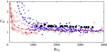
. The ratio of current speed to the maximum flow speed in waves lies between 0 and 2.3. As shown in figure 3, the results for both emergent and submerged canopies under pure waves and wave–current combinations are hardly distinguishable, and the averaged drag coefficient can be summarized by the single formula
 $$\begin{eqnarray}C_{Dave}=1.04+\left(\frac{730}{\mathit{Re}_{d}}\right)^{1.37},\quad 300<\mathit{Re}_{d}<4700,\end{eqnarray}$$
which does not reveal any dependence on the solid fraction. It should be noted also that the scattered data for
 $C_{D}$
for pure waves in the range
 $\mathit{Re}_{d}<1400$
are in general greater than those for pure current. At higher
 $\mathit{Re}_{d}$
all data by Hu et al. (Reference Hu, Suzuki, Zitman, Uittewaal and Stive2014) are for waves riding on a current. In that range (8.6) and (8.4) virtually coincide, as shown in figure 3. This indicates that the addition of a current to waves tends to reduce vegetation resistance.
Comparison of drag coefficients. Dashed line:
 $C_{Dave}$
according to (8.6) for
 $300<Re<4700$
including both pure waves and wave–current combinations. The crosses represent data of Hu et al. (Reference Hu, Suzuki, Zitman, Uittewaal and Stive2014) for pure waves, and asterisks their data for waves on a current. Dashed-dot line:
 $C_{Dave}$
according to (8.4) for pure current with
 ${\it\varphi}=0.049$
. The squares represent the upper bounds and the diamonds the lower bounds of the scattered data of Cheng & Nguyen (Reference Cheng and Nguyen2011). The dark dots represent the canopy-averaged
 ${C_{D}}_{L}={\it\alpha}\langle C_{Dave}\rangle _{L}$
used for simulation of our experiments.

Similar drag reduction has been noted in experiments for offshore towers by Allender & Petrauskas (Reference Allender and Petrauskas1987). Recently, Santo et al. (Reference Santo, Taylor, Williamson and Choo2014) conducted experiments for perforated plates normal to the direction of oncoming waves and currents. They found that when the solid fraction
 $A/A_{f}$
is small,
 $C_{D}$
decreases if the ratio
 $u_{c}/u_{w}$
increases, where
 $A$
is the solid area,
 $A_{f}$
is the frontal area of the perforated plates,
 $u_{c}$
is the current velocity and
 $u_{w}$
is the maximum wave velocity (see table 6 for
 $A/A_{f}=0.15$
in Santo et al. (Reference Santo, Taylor, Williamson and Choo2014)).
It may be remarked that drag reduction due to the addition of current to waves is already known for isolated piles. Sarpkaya (Reference Sarpkaya2010) (see figure 3.34 on p. 103) has given experimental evidence that the drop depends on the Keulegan–Carpenter number
 $\mathit{KC}=\langle U^{\prime }\rangle T/d^{\prime }$
, where
 $T$
is the wave period. Bearman, Graham & Singh (Reference Bearman, Graham, Singh and Shaw1979) also showed for a circular cylinder in plane oscillatory flow that for
 $\mathit{KC}$
between 10 and 20 (roughly the same range as in our canopy experiments, as shown in table 2), the ratio of
 $C_{D}/C_{D}^{\infty }$
is approximately 1.71 and 1.35, where
 $C_{D}^{\infty }$
is the steady-current value. This ratio decreases with increasing
 $\mathit{KC}$
. At approximately
 $\mathit{KC}=50$
,
 $C_{D}$
is only slightly higher than
 $C_{D}^{\infty }$
, see Faltinsen (Reference Faltinsen1990) for a review.
Lacking force measurements in our wave experiments, to be described shortly, we choose
 $C_{D}={\it\alpha}C_{Dave}$
in our numerical simulations, where
 $C_{Dave}$
is given by (8.4) for steady currents. The factor
 ${\it\alpha}=O(1)$
is chosen to match the wave data at one station, based on which predictions are made for 10 other stations. Detailed comparisons with the wave experiments will be discussed later.
To obtain a more explicit form for the left-hand side of (8.3), we first calculate the mean velocity from (6.8),
 $$\begin{eqnarray}\langle \widetilde{u}^{(0)}\rangle =-\text{Re}\left(\mathscr{K}\frac{\partial P^{(0)}}{\partial x}\text{e}^{-\text{i}t}\right).\end{eqnarray}$$
Using (3.13) and
 ${\it\phi}={\it\phi}^{(0)}+O({\it\epsilon})={\it\psi}^{(0)}\text{e}^{\text{i}S/{\it\epsilon}}+O({\it\epsilon})$
to the leading order, we obtain
 $$\begin{eqnarray}\frac{\partial P^{(0)}}{\partial x}\text{e}^{-\text{i}t}=\text{i}\left[\frac{\partial {\it\phi}^{(0)}}{\partial x}\right]_{-h}\text{e}^{-\text{i}t}=-k\left[{\it\psi}^{(0)}\right]_{-h}\text{e}^{\text{i}S/{\it\epsilon}-\text{i}t}=\frac{\text{i}kA(X)}{\cosh kh}\text{e}^{\text{i}S/{\it\epsilon}-\text{i}t}.\end{eqnarray}$$
Hence,
 $$\begin{eqnarray}\langle \widetilde{u}^{(0)}\rangle =-\text{Re}\left[\mathscr{K}\frac{\partial P^{(0)}}{\partial x}\text{e}^{-\text{i}t}\right]=-\text{Re}\left[\frac{\text{i}k\mathscr{K}A}{\cosh kh}\text{e}^{\text{i}(S/{\it\epsilon}-t)}\right]=\frac{k|\mathscr{K}|\,|A|}{\cosh kh}\cos {\it\Theta},\end{eqnarray}$$
where
 $$\begin{eqnarray}{\it\Theta}=S/{\it\epsilon}-t+{\it\theta}_{K}=\frac{1}{{\it\epsilon}}\int ^{X}k\text{d}X-t+{\it\theta}_{K}\end{eqnarray}$$
and
 ${\it\theta}_{K}$
is the phase of
 $-\text{i}\mathscr{K}A$
. The period average on the right-hand side of (8.2) is
 $$\begin{eqnarray}C_{D}\left(\frac{k|\mathscr{K}|\,|A|}{\cosh kh}\right)^{3}\overline{\cos ^{2}{\it\Theta}|\cos {\it\Theta}|}=C_{D}\left(\frac{k|\mathscr{K}|\,|A|}{\cosh kh}\right)^{3}\frac{4}{3{\rm\pi}}.\end{eqnarray}$$
On the other hand, the dissipation rate on the left-hand side is
 $$\begin{eqnarray}\displaystyle & & \displaystyle \frac{1}{2}\iint _{{\it\Omega}_{f}}\text{d}{\it\xi}\text{d}{\it\zeta}\overline{\left(\frac{\partial \widetilde{u}_{i}^{(0)}}{\partial {\it\xi}_{j}}+\frac{\partial \widetilde{u}_{j}^{(0)}}{\partial {\it\xi}_{i}}\right)^{2}}\nonumber\\ \displaystyle & & \displaystyle \quad =\iint _{{\it\Omega}_{f}}\text{d}{\it\xi}\text{d}{\it\zeta}\overline{\left\{2\left[\left(\frac{\partial \widetilde{u}^{(0)}}{\partial {\it\xi}}\right)^{2}+\left(\frac{\partial \widetilde{v}^{(0)}}{\partial {\it\eta}}\right)^{2}\right]+\left(\frac{\partial \widetilde{v}^{(0)}}{\partial {\it\xi}}+\frac{\partial \widetilde{u}^{(0)}}{\partial {\it\eta}}\right)^{2}\right\}},\end{eqnarray}$$
since
 $$\begin{eqnarray}\widetilde{u}^{(0)}=-\text{Re}\left(\unicode[STIX]{x1D612}_{11}\frac{\partial P^{(0)}}{\partial x}\text{e}^{-\text{i}t}\right),\quad \widetilde{v}^{(0)}=-\text{Re}\left(\unicode[STIX]{x1D612}_{21}\frac{\partial P^{(0)}}{\partial x}\text{e}^{-\text{i}t}\right).\end{eqnarray}$$
After straightforward calculations an implicit equation for
 ${\it\nu}_{t}$
is found,
 $$\begin{eqnarray}\frac{{\it\nu}_{t}}{{\it\omega}A_{0}d}=\frac{\displaystyle C_{D}\left(\frac{k|\mathscr{K}|\,|A|}{\cosh kh}\right)^{3}\frac{2}{3{\rm\pi}}}{\displaystyle \iint _{{\it\Omega}_{f}}\text{d}{\it\xi}\text{d}{\it\zeta}\left\{\left|\frac{\partial \unicode[STIX]{x1D612}_{11}}{\partial {\it\xi}}\right|^{2}\!+\left|\frac{\partial \unicode[STIX]{x1D612}_{21}}{\partial {\it\xi}}\right|^{2}\!+\frac{1}{2}\left|\frac{\partial \unicode[STIX]{x1D612}_{11}}{\partial {\it\eta}}\right|^{2}\!+\frac{1}{2}\left|\frac{\partial \unicode[STIX]{x1D612}_{21}}{\partial {\it\eta}}\right|^{2}\!+\text{Re}\left[\frac{\partial K_{11}^{\ast }}{\partial {\it\eta}}\frac{\partial \unicode[STIX]{x1D612}_{21}}{\partial {\it\xi}}\right]\!\right\}},\end{eqnarray}$$
which is solved iteratively from the interstitial velocities. Herein,
 $\unicode[STIX]{x1D612}_{ij}^{\ast }$
is the conjugate of
 $\unicode[STIX]{x1D612}_{ij}$
. This result also shows that
 ${\it\nu}_{t}$
varies slowly in space through the macroscale coordinate
 $X$
.
It should be noted from (8.4) that
 $C_{D}$
depends on
 $|\langle U^{\prime }\rangle |=|\langle \widetilde{u}^{(0)}\rangle ^{\prime }|$
nonlinearly through
 $\mathit{Re}_{v}$
. It should be noted also that
 ${\it\sigma}$
depends nonlinearly on the local wave amplitude
 $A(X)$
.
9. Experiments for waves over a canopy on a horizontal seabed
Laboratory experiments have been conducted in a wave flume of length 55 m and width 0.8 m at Shanghai Jiao Tong University, China. The water depth was kept at
 $h_{0}^{\prime }=0.5~\text{m}$
. Monochromatic waves were generated by a piston at one end of the flume. At the opposite end a beach of 1:6 slope was covered with a porous material for wave absorption. The model canopy was a square array of aluminium cylinders of diameter
 $d^{\prime }=2~\text{cm}$
and height
 $H^{\prime }=12~\text{cm}$
. Spaced at
 $\ell ^{\prime }=8~\text{cm}$
apart, 1250 cylinders covered the full flume width and the total length of 10.0 m, roughly 4–10 times the wavelength tested. In order to produce significant attenuation within the range of 10 m, the ratio
 $H^{\prime }/(h^{\prime }+H^{\prime })=0.24$
was chosen to be only moderately small. The porosity was
 $n=1-{\it\varphi}=1-0.04909=0.9509$
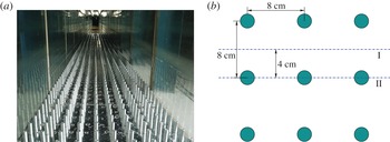
. The set-up is shown in figures 4 and 5.
The set-up of the wave flume and canopy.

(a) Front view of the canopy. (b) Top view of the cylinder array. Station II marks the light sheet for photography.

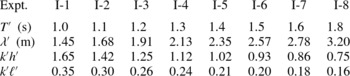
Free-surface displacements were recorded by 11 capacitance gauges along the canopy at 1 m spacings. Eight sets of tests were conducted with wave periods ranging from
 $T^{\prime }=1.0$
to 1.8 s. For each period, three incident amplitudes were tested,
 $A_{0}^{\prime }=2.5$
, 3.75 and 5 cm. Each test was repeated three times. The wave parameters are listed in table 1. No force measurements were taken.
Incident wave parameters in the experiments:
 $T^{\prime }=\text{wave}$
period,
 ${\it\lambda}^{\prime }=2{\rm\pi}/k^{\prime }=\text{wavelength}$
and
 $k^{\prime }=\text{wavenumber}$
. Total water depth
 $h_{0}^{\prime }=0.50~\text{m}$
, cylinder height
 $H^{\prime }=0.12~\text{m}$
. For each wave period three wave amplitudes were tested,
 $A_{0}^{\prime }=2.5$
, 3.75 and 5.0 cm.

The beach was far enough from the canopy so that steady periodic waves were established at all gauges before reflection from the beach was felt at the last gauge G11. By using free-surface data at gauges G1 and G2, the reflection coefficient on the incidence side was found to be small, as assumed in the theory due to the smallness of
 $k^{\prime }H^{\prime }$
and the volume fraction.
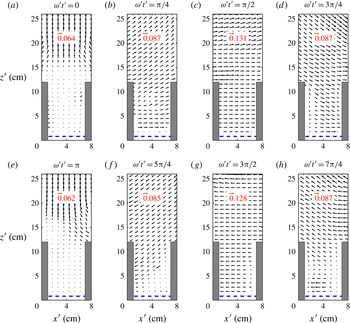
The velocity field measured at station II at different instants
 ${\it\omega}^{\prime }t^{\prime }$
for
 $T^{\prime }=1.5~\text{s}$
and
 $A_{0}^{\prime }=5~\text{cm}$
, the largest amplitude tested.

Steady currents over vegetation canopies are known to induce vortices due to Kelvin–Helmholtz instability, manifested by the wave-like motion in wheat fields on windy days. In experiments by Ghisalberti & Schlosser (Reference Ghisalberti and Schlosser2013) for a very long-period wave over a canopy of vertical cylinders, vortices have also been observed when the horizontal velocity above reverses direction, if the Keulegan–Carpenter and Reynolds numbers are sufficiently large. In order to see whether such vortex formation is important in the present study of relatively short water waves, PIV images of the flow in the vertical light sheet at station II were recorded from the side wall (see figure 5). The spatial resolution was
 $8.1~\text{mm}\times 8.1~\text{mm}$
, which could filter the turbulent fluctuations. Using a framing rate of 112 Hz and an exposure time of
 $7~{\rm\mu}\text{s}$
, the mean velocity fields at desired instants were obtained by using the phase-averaged images in 5–7 wave periods. Figure 6 shows snapshots of the velocity field recorded at intervals
 ${\rm\Delta}({\it\omega}^{\prime }t^{\prime })={\rm\pi}/4$
for the largest initial amplitude. Below the dashed line no velocity data could be resolved due to light reflection by the aluminium bottom. For legibility the velocity vectors are differently magnified, as indicated in each snapshot. Under a crest (
 ${\it\omega}^{\prime }t^{\prime }={\rm\pi}/2$
) or a trough (
 ${\it\omega}^{\prime }t^{\prime }=3{\rm\pi}/2$
), the velocity vectors are essentially horizontal. Under a wave node (
 ${\it\omega}^{\prime }t^{\prime }=0,{\rm\pi}$
) the velocity vectors are nearly vertical above the cylinders and nearly zero between the cylinders. No significant separation or vortex formation is seen at any time, as assumed in the theory. Because the dimensionless permeability (
 $\text{Im}\mathscr{K}$
) is just slightly less than unity, as shown in table 2, slippage at the canopy top is weak, which does not lead to shear instability in a short time. This explains why the flow just above the canopy is quite smooth even when the horizontal velocity is the greatest. Equivalently, these results are associated with the smallness of the Keulegan–Carpenter number, as will be discussed further later.
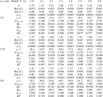
Parameters for calculating the eddy viscosity by the energy criterion. Total water depth
 $h_{0}^{\prime }=0.5~\text{m}$
, cylinder height
 $H^{\prime }=0.12~\text{m}$
,
 ${\it\nu}_{t}={\it\omega}^{\prime }\ell ^{\prime 2}{\it\sigma}$
. Here,
 $\mathscr{K}$
is the normalized complex permeability,
 $\mathit{Re}_{v}$
is defined in (8.5a,b
),
 $\mathit{Re}_{d}=\langle U^{\prime }\rangle d^{\prime }/{\it\nu}$
,
 ${C_{D}}_{L}={\it\alpha}\langle C_{Dave}\rangle _{L}$
and
 $\mathit{KC}$
is the Keulegan–Carpenter number defined in (10.1), where
 ${C_{D}}_{L}$
is the drag coefficient. (Using
 $C_{D}$
for an isolated cylinder gives smaller
 $\mathit{KC}$
.) All quantities listed in the table are averages along the canopy.

10. Computation of the eddy viscosity and simulation of the experiments
For each experiment, the eddy viscosity
 ${\it\nu}_{t}(X)$
depends on the local value of
 $A(X)$
. Therefore, the following iteration procedure is used.
-
(a) In the canopy region
 $0\leqslant X\leqslant L$
, equally spaced interior stations
$X_{n}$
:
$0=X_{1}<\cdots <X_{n}<\cdots <X_{N}=L$
are chosen. As the initial guess we set
$\langle U^{(0)}(X_{n})\rangle ={\it\omega}A_{0}$
for all the interior stations. Equation (8.1) is used to choose the first
${\it\nu}_{t}^{(0)}$
, hence
${\it\sigma}^{(0)}(X_{n})={\it\nu}_{t}/{\it\omega}\ell ^{2}$
. The cell problem for
$\unicode[STIX]{x1D612}_{ij}^{(0)}$
and
$B_{j}^{(0)}$
at each location
$X_{n}$
is solved by the finite element method.
-
(b) When
$\unicode[STIX]{x1D612}_{ij}^{(i-1)}(X_{n})$
and
$B_{j}^{(i-1)}(X_{n})$
are obtained at every station after
$i-1$
iterations, cell averages are taken to obtain
$\mathscr{K}^{(i-1)}(X_{n})=\langle \unicode[STIX]{x1D612}_{ij}^{(i-1)}(X_{n})\rangle$
. The local wave amplitude
$A^{(i)}(X_{n})$
along the canopy is updated according to (7.21) for all
$X_{n}$
. Using (8.9) we obtain the cell-averaged velocity
$\langle U^{(i)}(X_{n})\rangle =k|\mathscr{K}(X_{n})|A(X_{n})/\text{cosh}\,kh$
inside the canopy region. Then the drag coefficient
$C_{Dave}^{(i)}(X_{n})$
is calculated from (8.4). Once
$A^{(i)}$
,
$\unicode[STIX]{x1D612}_{ij}^{(i)}$
and
${C_{Dave}}^{(i)}$
are known, the local eddy viscosity
${\it\nu}_{t}^{(i)}$
at
$X_{n}$
is calculated from the implicit equation (8.14) by iteration. Requiring
$|{\it\nu}_{t}^{(i)}(X_{n})-{\it\nu}_{t}^{(i-1)}(X_{n})|/{\it\nu}_{t}^{(i)}(X_{n})<10^{-3}$
for convergence at each station, the final wave amplitude
$A^{(i)}(X_{n})$
is found. -
(c) A fitting coefficient
${\it\alpha}$
is chosen so that
$C_{D}={\it\alpha}C_{Dave}$
; the computed wave amplitude at the final station
$A(X_{N})$
equals the measured value
$[A(X_{N})]_{exp}$
.

















After finding
 ${\it\alpha}$
for good fitting at the final station, the same
 ${\it\alpha}$
is used to predict
 $A(X_{n})$
at all other stations for comparison with measured data. For all test cases the values of
 ${\it\alpha}$
are listed in table 2.
By using
 $C_{Dave}$
calculated from (8.4) with the fitting parameter
 ${\it\alpha}$
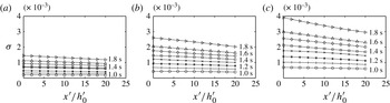
listed in table 2, the corresponding dimensionless eddy viscosity is plotted in figure 7. Clearly,
 ${\it\sigma}$
decreases weakly in the direction of wave propagation along the canopy. The decrease is greater for longer wave periods and/or higher initial amplitudes.
The dimensionless eddy viscosity
 ${\it\sigma}={\it\nu}_{t}/{\it\omega}^{\prime }{\ell ^{\prime }}^{2}$
along the canopy region for
 ${\it\omega}^{\prime }t^{\prime }=1.0,\dots ,1.8~\text{s}$
and three incident wave amplitudes: (a)
 $A_{0}^{\prime }=2.5~\text{cm}$
; (b)
 $A_{0}^{\prime }=3.75~\text{cm}$
; (c)
 $A_{0}^{\prime }=5.0~\text{cm}$
. Total water depth:
 $h_{0}^{\prime }=0.5~\text{m}$
. Cylinder height:
 $H^{\prime }=0.12~\text{m}$
.

For reference we list in table 2 the values of
 $\langle {\it\sigma}\rangle _{L}$
and
 $\langle C_{Dave}\rangle _{L}$
, which are averages over the entire canopy length
 $L$
. It can be seen that the eddy viscosity and the drag coefficient decrease with decreasing wave period and increasing Reynolds number, as is known for a single cylinder (see Sarpkaya Reference Sarpkaya2010, p. 82).
In the experiments of Ghisalberti & Schlosser (Reference Ghisalberti and Schlosser2013), visual records are taken for standing waves of long periods
 $T=12.5{-}80~\text{s}$
. In terms of the Keulegan–Carpenter number
 $$\begin{eqnarray}\mathit{KC}=\frac{U_{0}^{\prime }T}{L_{D}},\quad L_{D}=\frac{{\rm\pi}(1-{\it\varphi})}{4C_{D}{\it\varphi}}d^{\prime },\end{eqnarray}$$
where
 $L_{D}$
is the drag length introduced by Coceal & Belcher (Reference Coceal and Belcher2004) and
 $C_{D}$
is calculated according to an empirical formula for an isolated cylinder, their tests were in the range of
 $3.5<\mathit{KC}<20$
. In some cases vortices were observed near the instants when the horizontal velocity reverses its direction. The threshold of the appearance of vortices was suggested to be
 $\mathit{KC}>5$
and
 $R_{e}^{gs}={U_{0}^{\prime }}^{2}T/2{\rm\pi}{\it\nu}>1000$
. Using
 ${C_{D}}_{L}$
for
 $C_{D}$
in (10.1), all our tests correspond to much smaller
 $\mathit{KC}$
than the suggested threshold, although our
 $R_{e}^{gs}$
values are mostly greater than 1000. (The ranges of
 $R_{e}^{gs}$
are (520, 2430) for
 $A_{0}^{\prime }=2.5~\text{cm}$
, (1200, 5200) for
 $A_{0}^{\prime }=3.75~\text{cm}$
and (2020, 8860) for
 $A_{0}=5.0~\text{cm}$
.) As the wave periods in Ghisalberti & Schlosser (Reference Ghisalberti and Schlosser2013) are much longer and the cylinder and canopy dimensions are quite different from ours, their suggested threshold may not be entirely applicable here. To establish a definitive criterion, more tests for a wider range of
 $\mathit{KC}$
and Reynolds numbers are needed to steer the theoretical treatment of the canopy top in stronger waves.
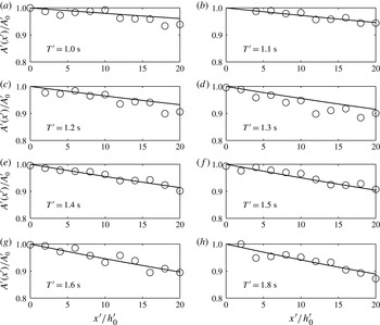
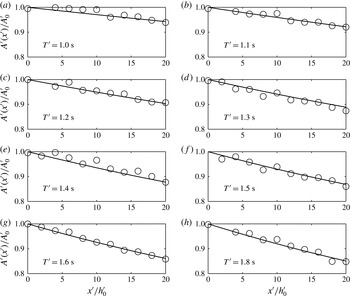
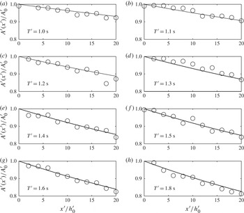
In figures 8–10 the calculated and measured wave amplitudes at all stations along the canopy are compared, for three incident amplitudes
 $A_{0}^{\prime }$
. The overall agreement is good. As expected, waves of longer period and/or larger amplitude are attenuated more quickly.
Comparison of the computed wave attenuation ratio (lines) with the measured data (circles) for
 $T^{\prime }=1.0,\dots ,1.8~\text{s}$
and
 $A_{0}^{\prime }=2.5~\text{cm}$
. Water depth:
 $h_{0}^{\prime }=0.5~\text{m}$
. Cylinder height:
 $H^{\prime }=0.12~\text{m}$
. Spacing:
 $\ell ^{\prime }=0.08~\text{m}$
. Total length of canopy:
 $L^{\prime }=10~\text{m}$
.

Comparison of the computed wave attenuation ratio (lines) with the measured data (circles) for
 $T^{\prime }=1.0,\dots ,1.8~\text{s}$
and
 $A_{0}^{\prime }=3.75~\text{cm}$
. Water depth:
 $h_{0}^{\prime }=0.5~\text{m}$
. Cylinder height:
 $H^{\prime }=0.12~\text{m}$
. Spacing:
 $\ell ^{\prime }=0.08~\text{m}$
. Total length of canopy:
 $L^{\prime }=10~\text{m}$
.

Comparison of the computed wave attenuation ratio (lines) with the measured data (circles) for
 $T^{\prime }=1.0,\dots ,1.8~\text{s}$
and
 $A_{0}^{\prime }=5.0~\text{cm}$
. Water depth:
 $h_{0}^{\prime }=0.5~\text{m}$
. Cylinder height:
 $H^{\prime }=0.12~\text{m}$
. Spacing:
 $\ell ^{\prime }=0.08~\text{m}$
. Total length of canopy:
 $L^{\prime }=10~\text{m}$
.

It should be noted that the fitting parameter
 ${\it\alpha}$
lies within the narrow range of 1.37–1.4, as listed in table 2. It is comforting that the fitted values of the canopy-averaged drag coefficient
 ${C_{D}}_{L}={\it\alpha}{C_{Dave}}_{L}$
fall within the scattered data around the mean value given by (8.4) and (8.6). In particular, for higher Reynolds numbers where no experiments are available for pure waves, our
 ${C_{D}}_{L}$
falls in the scattered range
 $1.31\pm 0.22$
given by Hu et al. (Reference Hu, Suzuki, Zitman, Uittewaal and Stive2014). That
 $C_{D}$
in waves is slightly greater than the mean values in a pure current or a current-dominated flow is consistent with the observed difference between the experiments by Cheng & Nguyen (Reference Cheng and Nguyen2011) and Hu et al. (Reference Hu, Suzuki, Zitman, Uittewaal and Stive2014). In view of the observations by Allender & Petrauskas (Reference Allender and Petrauskas1987) and Santo et al. (Reference Santo, Taylor, Williamson and Choo2014), it can be expected that future measurements of the forces on cylinders in waves for a wider range of Reynolds numbers would provide values of
 $C_{D}$
directly usable in our scheme without fitting.
The agreement in figures 8–10 gives encouraging confirmation of the microscale model based on the constant eddy viscosity and the energy argument. New experimental information on
 $C_{D}$
by force measurements for pure waves with higher amplitudes is certainly desirable for further confirmation.
11. Effects of wave frequency, solid fraction and bed slope
We next explore wave attenuation for a broad range of wave frequency, solid fraction and bed slope, for a simple bathymetry of large scale. For field applications it is necessary to account for seabed friction, which depends on the seabed roughness. For turbulent flow over rough seabeds, the value of
 $f_{w}$
can reach a value as high as 0.05, depending on the ratio between the free stream orbital amplitude and the roughness height. In the following examples we assume the seabed to be covered by fine sand without ripples or bars. The bottom friction coefficient is then around
 $f_{w}=0.01$
, which is used to calculate the ratio
 ${\it\beta}$
in (4.9a,b
).
Let us first consider a horizontal seabed of total depth
 $h_{0}^{\prime }=10~\text{m}$
. A periodic wave of amplitude
 $A_{0}^{\prime }=0.5~\text{m}$
and fixed wavelength
 $k_{0}^{\prime }h_{0}^{\prime }$
enters a canopy of height
 $H^{\prime }=1.0~\text{m}$
and cylinder spacing (
 $=\text{lattice constant}$
)
 $\ell ^{\prime }=1.0~\text{m}$
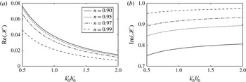
. The real and imaginary parts of the dimensionless permeability
 $\mathscr{K}$
are shown in figure 11 for four porosities
 $n=1-{\it\varphi}=0.90$
, 0.95, 0.97 and 0.99, corresponding to
 $d^{\prime }/\ell ^{\prime }\approx 0.36$
, 0.25, 0.20 and 0.11. From the behaviour of
 $\text{Re}(\mathscr{K})$
it is seen that the decay is faster for longer waves for the same porosity, and with decreasing porosity for the same wavelength.
Effects of the porosity
 $n=1-{\it\varphi}$
and wavelength
 $k_{0}h_{0}$
on the non-dimensional permeability
 $\mathscr{K}$
for a horizontal seabed. The parameters are total water depth
 $h_{0}^{\prime }=10~\text{m}$
, canopy height
 $H^{\prime }=1~\text{m}$
, canopy spacing
 $\ell ^{\prime }=1.0~\text{m}$
, wave amplitude
 $A_{0}^{\prime }=0.5~\text{m}$
and
 $f_{w}=0.01$
.

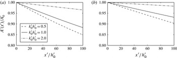
For two porosities, the rates of wave attenuation are compared in figure 11 for three different wavelengths. The spatial decay is essentially linear rather than exponential, due to the nonlinear variation of the eddy viscosity.
The spatial variation of
 $A=A^{\prime }(x^{\prime })/A_{0}^{\prime }$
in the direction of the waves is shown in figure 12. For the same canopy and water depth, longer waves (smaller
 $k_{0}h_{0}$
) are damped more quickly, of course.
Attenuation of the wave amplitude
 $A(x)/A_{0}$
versus the non-dimensional distance
 $x^{\prime }/h_{0}^{\prime }$
for different wavelengths
 $k_{0}^{\prime }h_{0}^{\prime }=0.5$
, 1.0 and 2.0 for a horizontal seabed. The porosity
 $n=0.90$
(a) and 0.99 (b). The input parameters are
 $h_{0}^{\prime }=10~\text{m}$
,
 $H^{\prime }=1.0~\text{m}$
,
 $\ell ^{\prime }=1.0~\text{m}$
,
 $A_{0}^{\prime }=0.5~\text{m}$
and
 $f_{w}=0.01$
.

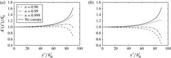
To examine the canopy effect on waves approaching a shore we consider a beach of
 $1/100$
slope, which begins offshore at the depth
 $h_{0}^{\prime }=20~\text{m}$
. The canopy height is constant,
 $H^{\prime }=1~\text{m}$
. Three canopies with porosities
 $n=1-{\it\varphi}=0.90$
, 0.99 and 0.999 are examined. Numerical results are shown only for
 $0<x^{\prime }/h_{0}^{\prime }<90$
. Closer to the shore,
 $80<x^{\prime }/h_{0}^{\prime }<100$
, the results are no longer reliable since the assumptions of a shallow canopy and linearization no longer hold. Nevertheless, the qualitative trend that a sufficiently dense canopy can totally annihilate incoming waves must be true.
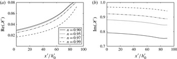
The shoreward variation of the dimensionless permeability
 $\mathscr{K}$
is plotted in figure 13. The attenuation of the wave amplitude according to (7.21) is shown in figure 14. Clearly, wave shoaling and canopy dissipation affect the wave amplitude in opposite ways. The case of pure shoaling without bottom friction or cylinders is also plotted for comparison. For a very sparse array with
 $n=0.999$
, the result for
 $A_{0}^{\prime }=0.50~\text{m}$
approaches the limit of pure shoaling on a plane beach without vegetation. A less sparse array with
 $n=0.99$
can provide significant shore damping of incoming waves, which no longer break.
Variation of the canopy permeability
 $\mathscr{K}$
versus
 $x^{\prime }/h_{0}^{\prime }$
across a beach for different vegetation porosities
 $n=1-{\it\varphi}$
. The input parameters are total depth
 $h_{0}^{\prime }=20~\text{m}$
, height of canopy
 $H^{\prime }=1.0~\text{m}$
, cylinder spacing
 $\ell ^{\prime }=2.0~\text{m}$
, incident wave amplitude
 $A_{0}^{\prime }=1.0~\text{m}$
,
 $k_{0}h_{0}=2{\rm\pi}/5$
and
 $f_{w}=0.01$
.

Amplitude attenuation
 $A/A_{0}$
across a sloping beach for different vegetation porosities
 $n=1-{\it\varphi}$
. The input parameters are total water depth
 $h_{0}^{\prime }=20~\text{m}$
, height of canopy
 $H^{\prime }=1.0~\text{m}$
, cylinder spacing
 $\ell ^{\prime }=2.0~\text{m}$
, depth-to-wavelength ratio
 $k_{0}^{\prime }h_{0}^{\prime }=2{\rm\pi}/5$
and
 $f_{w}=0.01$
, for (a)
 $A_{0}^{\prime }=0.5~\text{m}$
, (b)
 $A_{0}^{\prime }=1.0~\text{m}$
.

Wave attenuation depends not only on the property of a shallow canopy, but also on the intensity of water motion, since both the turbulent dissipation inside the canopy region and the bottom friction depend on the Reynolds number. A quantitative comparison in given in figure 13 for two wave amplitudes,
 $A^{\prime }=1.0~\text{m}$
and
 $A^{\prime }=0.5~\text{m}$
. For a sufficiently dense canopy, both waves are damped out near the shore.
The preceding results suggest that the idea of a green forest for tsunami protection described by Hiraishi & Harada (Reference Hiraishi and Harada2003) may be reasonable on scientific grounds, although more study for stronger waves and their effects on plant deformation or even uprooting is needed. The practical feasibility depends, of course, also on economical and environmental considerations.
12. Concluding remarks
The attenuation of gravity waves by a submerged shallow canopy is theoretically analysed, based on the dynamics on a small scale comparable to plant spacing. Within the framework of small-amplitude waves, two assumptions are made to minimize the computational task. The first is to model the canopy as a periodic array of rigid cylinders. This is probably a gross simplification for coral reefs, mangroves or kelps in nature, but may provide qualitative insight for their macroscale effects. The second is the assumption of constant eddy viscosity, which requires much less numerical effort in comparison with RANS or LES schemes, but gives insight into the physics and is qualitatively consistent with the experimental evidence for an isolated object in a turbulent free stream (Wu & Faeth Reference Wu and Faeth1994a ,Reference Wu and Faeth b ). As an improvement over Mei et al. (Reference Mei, Chan, Liu, Huang and Zhang2011), the constant eddy viscosity is computed, not estimated by order-of-magnitude, from the requirement that the work done by the drag force on the array equals the rate of dissipation inside. Using the available data on the drag force in steady flow and in pure waves, the asymptotic method of multiple scales enables us to make reasonable predictions of wave attenuation over much greater scales with relatively modest numerical effort.
The general scheme of this article has recently been applied by Liu et al. (Reference Liu, Chang, Mei, Lomonaco, Martin and Maza2015) to infinitesimal waves through an emergent array, both one- and two-dimensional, on a horizontal seabed, and to a strong steady current through an emergent array in an open channel (Guo, Wang & Mei Reference Guo, Wang and Mei2014). In the latter work convective inertia is important in the cell problem and nonlinear corrections to the classical Darcy’s law are derived. The computed interstitial flow is then used to predict the Taylor dispersion of solutes in the array. An immediate extension of the present work is to consider waves over canopies of any height, for which the analysis must include the effects of scattering. In order to predict the interaction of coastal vegetation with storm surges and tsunamis, it is necessary to consider transient waves of large amplitude. Nonlinearity and shear-induced vortices on the canopy top must then be accounted for. In addition, there are many other theoretical challenges such as the deformability of vegetation stems and the irregularity of their geometries. More comprehensive experiments examining these aspects for regular or random waves and arrays will of course be essential.
Acknowledgements
This research has been partially funded by the Natural Science Foundation of China (grant nos 11202129, 11272210). C.C.M. acknowledges the support by Shanghai Jiao Tong University for a visiting professorship, and the hospitality of Tianjin University.